1 23

Climatic ChangeAn Interdisciplinary, InternationalJournal Devoted to the Description,Causes and Implications of ClimaticChange ISSN 0165-0009 Climatic ChangeDOI 10.1007/s10584-015-1377-3

Modeling sea-level rise vulnerabilityof coastal environments using rankedmanagement concerns

Haunani H. Kane, Charles H. Fletcher,L. Neil Frazer, Tiffany R. Anderson &Matthew M. Barbee

1 23

Your article is protected by copyright and all

rights are held exclusively by Springer Science

+Business Media Dordrecht. This e-offprint

is for personal use only and shall not be self-

archived in electronic repositories. If you wish

to self-archive your article, please use the

accepted manuscript version for posting on

your own website. You may further deposit

the accepted manuscript version in any

repository, provided it is only made publicly

available 12 months after official publication

or later and provided acknowledgement is

given to the original source of publication

and a link is inserted to the published article

on Springer's website. The link must be

accompanied by the following text: "The final

publication is available at link.springer.com”.

Modeling sea-level rise vulnerability of coastalenvironments using ranked management concerns

Haunani H. Kane & Charles H. Fletcher & L. Neil Frazer &

Tiffany R. Anderson & Matthew M. Barbee

Received: 11 April 2014 /Accepted: 1 March 2015# Springer Science+Business Media Dordrecht 2015

Abstract Coastal erosion, salt-water intrusion, and flooding due to sea-level rise threaten todegrade critical coastal strand and wetland habitats. Because habitat loss is a measure of therisk of extinction, managers are keen for guidance to reduce risk posed by sea-level rise.Building upon standard inundation mapping techniques and suitability mapping, we develop aranking system that models sea-level rise vulnerability as a function of six input parametersdefined by wetland experts: type of inundation, time of inundation, soil type, habitat value,infrastructure, and coastal erosion. We apply this model under the mid-century and end-of-century RCP8.5 sea-level projection (0.30 m by 2057, and 0.74 m by 2100) according to theIntergovernmental Panel on Climate Change Fifth Assessment Report. To demonstrate thismethod, the model is applied to three coastal wetlands on the Hawaiian islands of Maui andO‘ahu. Each ranked input parameter is mapped upon a 2 m horizontal resolution raster andfinal vulnerability is obtained by calculating the weighted geometric mean of the inputvulnerability scores. Areas that ranked with the ‘highest’ vulnerability should be the focusof future management efforts. The tools developed in this study can be a guide to prioritizeconservation actions at flooded areas and initiate decisions to adaptively manage sea-level riseimpacts.

1 Introduction

Globally, coastal strand and wetland habitats have high conservation value due to the role theyplay in the preservation of endangered and endemic organisms. Wetlands provide a variety offunctions that reduce storm damage and stabilize shorelines (Gedan et al. 2011), trap land-based sediments, retain nutrients, and alleviate flooding (Bruland 2008). In the Pacific regionalone, over 2500 islands and atolls harbor a diverse range of freshwater, coastal, and marinewetlands (Ellison 2009). It is noted that the disappearance of small wetlands will cause a dire

Climatic ChangeDOI 10.1007/s10584-015-1377-3

Electronic supplementary material The online version of this article (doi:10.1007/s10584-015-1377-3)contains supplementary material, which is available to authorized users.

H. H. Kane (*) : C. H. Fletcher : L. N. Frazer : T. R. Anderson :M. M. BarbeeSOEST/Geology and Geophysics, University of Hawai‘i, 1680 East West Road, Honolulu, HI 96822, USAe-mail: hkane@hawaii.edu

Author's personal copy

reduction in the ecological connection among remaining species populations (Semlitsch andBodie 1998).

Sea-level rise (SLR) is a growing problem on low lying coastal plains and threatens costalstrand and wetland habitats with increased erosion (Romine et al. 2013), frequency of extremehigh water events (Tebaldi et al. 2012), pond water levels, and salinity (Kuan et al. 2012). TheIntergovernmental Panel on Climate Change (IPCC) Fifth Assessment Report (AR5) predictsunder a worst case scenario (RCP8.5), global sea-level will increase 0.30±0.08 m by 2057(mid-century) and 0.74±0.23 m by 2100 relative to 1986–2005 (Church et al. 2013). Equa-torial Pacific regions may experience sea-level values between 10 and 20% above the globalmean (IPCC 2013). Islands within the tropics are especially vulnerable because species havenarrow tolerances for changes in climate (Mora et al. 2013), and microtidal (<2 m tidal range)environments do not allow for large concentrations of marine suspended sediment to aid invertical accretion in response to SLR (Kirwan et al. 2010).

To date, much of insular SLR vulnerability research has focused on summarizing potentialimpacts on a global scale (e.g., Wetzel et al. 2012; Bellard et al. 2013). For example, Bellardet al. (2013) found that approximately 6% of the 4447 islands investigated worldwidewould be entirely submerged under 1 m of SLR. Global assessments are beneficial fordemonstrating the general consequences of SLR, however through the use of low resolutionelevation data sets, the final vulnerability maps are produced with large errors (Cooperet al. 2013b). Furthermore most management occurs at regional and local scales, thusfine-scale vulnerability assessments are more relevant for direct decision making(Halpern et al. 2007).

Prior regional scale assessments define SLR vulnerability based upon uncertainty in high-resolution elevation along with tidal datums (Gesch 2013) and SLR estimates (Cooper andChen 2013). However within highly managed areas such as Hawaiian wetlands, landscapevulnerability should relate to the site-specific goals of decision makers. Previous studies havegained stakeholder’s support by ranking the vulnerability of marine ecosystems to anthropo-genic threats based on survey results of experts (e.g., Halpern et al. 2007; Fuentes andCinner 2010; Selkoe et al. 2008). These studies employ an expert elicitation processthat involves synthesizing expert’s opinion of relative impacts and assessing the uncertainty ofthose views (Halpern et al. 2007; Fuentes and Cinner 2010). Expert knowledge isused both in instances when data is scarce, and to supplement empirical data (Hameedet al. 2013). To aid in the prioritization of conservation actions those ecosystemthreats that are identified as having the greatest impact generally are dealt with first(Fuentes and Cinner 2010).

Most threat ranking studies to date include SLR in an array of multiple stressors, and do notprovide maps that spatially represent areas assumed to experience the greatest impacts.Previous studies have generated suitability maps that use ranked variables to identifypotential wetland mitigation and restoration sites (Van Lonkhuyzen et al. 2004; Whiteand Fennessy 2005). Integrating expert elicitation with suitability mapping in a GISwould allow decision makers with site-specific goals to evaluate landscape vulnerability due tofuture SLR.

We present an important case study that depicts a localized approach to prioritizingmanagement strategies in response to SLR based upon a number of predetermined factorssuch as the time and nature of flooding, environmental features that influence flood severity,and the loss that would result from flooded high value habitats and infrastructure. Thevulnerability ranking process may be easily refined and replicated to other small, microtidalislands to accommodate different planning needs, data availability, and sources of expertknowledge.

Climatic Change

Author's personal copy

2 Methods

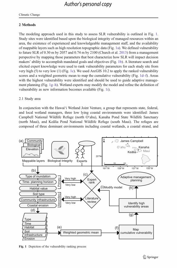
The modeling approach used in this study to assess SLR vulnerability is outlined in Fig. 1.Study sites were identified based upon the biological integrity of managed resources within anarea, the existence of experienced and knowledgeable management staff, and the availabilityof mappable layers such as high resolution topographic data (Fig. 1a). We defined vulnerabilityto future SLR of 0.30 m by 2057 and 0.74 m by 2100 (Church et al. 2013) from a managementperspective by mapping those parameters that best characterize how SLR will impact decisionmakers’ ability to accomplish mandated goals and objectives (Fig. 1b). A literature search andelicited expert knowledge were used to rank vulnerability parameters for each study site fromvery high (5) to very low (1) (Fig. 1c). We used ArcGIS 10.2 to apply the ranked vulnerabilityscores and a weighted geometric mean to map the cumulative vulnerability (Fig. 1d–f). Areaswith the highest vulnerability were identified and should be used to guide adaptive manage-ment planning (Fig. 1g–h). Wetland experts may modify the model and refine the definition ofvulnerability as new information becomes available (Fig. 1i).

2.1 Study area

In conjunction with the Hawai‘i Wetland Joint Venture, a group that represents state, federal,and local wetland managers, three low lying coastal environments were identified: JamesCampbell National Wildlife Refuge (north O‘ahu), Kanaha Pond State Wildlife Sanctuary(north Maui), and Keālia Pond National Wildlife Refuge (south Maui). The refuges arecomposed of three dominant environments including coastal wetlands, a coastal strand, and

Erosion

ElevationBiologicalCommunity

Biological Integrity Experts

rankVery high

Very low

TypeTimeHabitat

Infrastructurecumulative vulnerability

Identify high

Mappable layers

Community infrastructure

Expert

(a)

(b)(c)

(d)

(e) (f)

(g)

(h)

Soil

Coastal erosion

Soil type

Habitat value

Time- planning horizon

Type of inundation

Weighted geometric mean

vulnerability areas

Adaptive management planning

Map

Modify model(i)

Literaturereview Identify high

cumulative vulnerability

Very high

Very low

Prim

ary

Seco

ndar

y

161°W 155°W157°W159°W

20°N

0030 150Km

O`ahuKeālia

Kanaha

James Campbell

Maui

N

Fig. 1 Depiction of the vulnerability ranking process

Climatic Change

Author's personal copy

upland habitats. The wetlands consist of freshwater impoundments and natural ponds that arefed by groundwater, and rainfall. The wetlands are largely buffered from marine flooding andsediment inputs by a narrow coastal strand and 2–4 m sand dunes (U.S. Fish and WildlifeService 2011a). The refuges provide habitats for the recovery of endangered waterbirds, theendangered Hawaiian monk seal (Monachus schauinslandi), the threatened Hawaiian greensea turtle (Chelonia mydas), seabirds, and migratory shorebirds. Identified at each study sitewere one to two senior wetland experts (four experts total) who from training, research, andpersonal experience (5–20+ years) possess the greatest capacity to assess how SLR will impactfuture management strategies.

2.2 Defining sea-level rise vulnerability

Here, we define SLR vulnerability as having primary and secondary parameters. Throughdiscussions with local wetland managers it was expressed that they are primarily concernedwith prioritizing management at flooded areas upon the value of each site. The primaryparameters are defined by 1) type of inundation, 2) time of inundation, and 3) habitat value.The secondary parameters refine the definition of threatened resources based upon theavailability of ancillary data. Secondary parameters are defined by 1) soil type, 2) communityinfrastructure, and 3) coastal erosion hazard zones.

2.3 Ranking vulnerability parameters

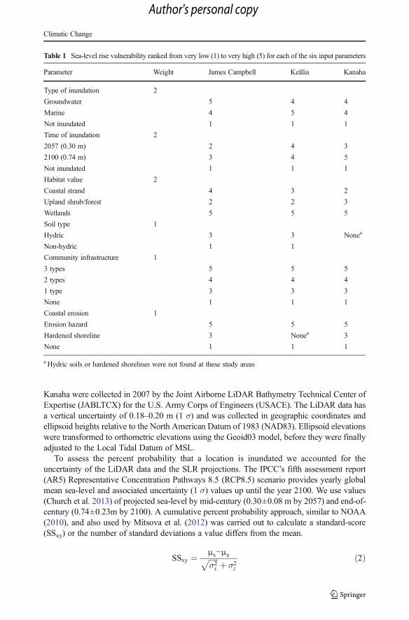
Expert judgment was used to rank the primary vulnerability parameters defined in Section 2.2.Face to face surveys were conducted and experts were asked a series of questions where theyranked the vulnerability of their refuge to SLR from very low (1) to very high (5) (Table 1).After each survey question, respondents were asked to use the same ranking scale to indicatehow confident they were about the depth of knowledge used to determine vulnerability(Halpern et al. 2007; Selkoe et al. 2008; Fuentes and Cinner 2010). Assessing surveyconfidence gives greater importance to values with higher certainty (Halpern et al. 2007),and allows for gaps in knowledge to be identified (e.g., low confidence responses). Equation 1defines vulnerability input rank as the summed product of vulnerability score and confidence,divided by the sum of the confidence.

Vulnerability InputRank ¼X

VulnerabilityScore� ConfidenceX

Confidenceð1Þ

Secondary input parameters were ranked by the authors, and relied on data collected from aliterature review. Secondary ranks were based upon the presence and intensity of the identifiedparameters. Secondary input parameters and their ranks are explained in more detail in thefollowing section.

2.4 Mapping vulnerability

GIS layers for each input parameter were compiled, and 2 m horizontal resolution rasters wereproduced such that each cell represented a corresponding vulnerability rank (Table 1). SLRinundation maps were generated by interpolating LiDAR ground returns as a 2 m horizontalresolution LiDAR DEM. The Federal Emergency Management Agency (FEMA) contractedAirborne 1 in 2006 to collect LiDAR data for Keālia, while LiDAR at James Campbell and

Climatic Change

Author's personal copy

Kanaha were collected in 2007 by the Joint Airborne LiDAR Bathymetry Technical Center ofExpertise (JABLTCX) for the U.S. Army Corps of Engineers (USACE). The LiDAR data hasa vertical uncertainty of 0.18–0.20 m (1 σ) and was collected in geographic coordinates andellipsoid heights relative to the North American Datum of 1983 (NAD83). Ellipsoid elevationswere transformed to orthometric elevations using the Geoid03 model, before they were finallyadjusted to the Local Tidal Datum of MSL.

To assess the percent probability that a location is inundated we accounted for theuncertainty of the LiDAR data and the SLR projections. The IPCC’s fifth assessment report(AR5) Representative Concentration Pathways 8.5 (RCP8.5) scenario provides yearly globalmean sea-level and associated uncertainty (1 σ) values up until the year 2100. We use values(Church et al. 2013) of projected sea-level by mid-century (0.30±0.08 m by 2057) and end-of-century (0.74±0.23m by 2100). A cumulative percent probability approach, similar to NOAA(2010), and also used by Mitsova et al. (2012) was carried out to calculate a standard-score(SSxy) or the number of standard deviations a value differs from the mean.

SSxy ¼ μs−μzffiffiffiffiffiσ2s

p þ σ2z

ð2Þ

Table 1 Sea-level rise vulnerability ranked from very low (1) to very high (5) for each of the six input parameters

Parameter Weight James Campbell Keālia Kanaha

Type of inundation 2

Groundwater 5 4 4

Marine 4 5 4

Not inundated 1 1 1

Time of inundation 2

2057 (0.30 m) 2 4 3

2100 (0.74 m) 3 4 5

Not inundated 1 1 1

Habitat value 2

Coastal strand 4 3 2

Upland shrub/forest 2 2 3

Wetlands 5 5 5

Soil type 1

Hydric 3 3 Nonea

Non-hydric 1 1

Community infrastructure 1

3 types 5 5 5

2 types 4 4 4

1 type 3 3 3

None 1 1 1

Coastal erosion 1

Erosion hazard 5 5 5

Hardened shoreline 3 Nonea 3

None 1 1 1

a Hydric soils or hardened shorelines were not found at these study areas

Climatic Change

Author's personal copy

The standard-score was calculated through a cell by cell approach where the differencebetween the projected sea-level value above MHHW (μs) and the DEM elevation (μz) wasdivided by the joint-uncertainty of SLR projections (σs) and LiDAR data (σz). The standardscore was converted to a percent probability via a look-up table. Similar to Cooper and Chen(2013) the probability rasters were reclassified by assigning the range of probability values 0–0.49 equal to 0 (not inundated), 0.50–0.79 equal to 50 (low probability), and 0.80–1 equal to80 (high probability).

One of the key issues for managing wetlands is identifying which areas may be impacted bymarine (salty) inundation or groundwater (potentially fresh or brackish) inundation as water-fowl and vegetation are sensitive to both increased pond water levels and salinity (U.S. Fishand Wildlife Service 2011a, b). To determine areas of marine inundation, DEM grid cellshydrologically connected to the ocean were identified using the 8-sided connectivity approach.This approach identifies those flooded cells that are either directly adjacent to the ocean orconnected to the ocean via adjacent grid cells in the cardinal and diagonal directions (Cooperet al. 2013b; Poulter and Haplin 2008). Inundated areas disconnected from the ocean wereassumed to be flooded by rising groundwater levels (Rotzoll and Fletcher 2012). Wetlandexperts ranked the vulnerability of their study area to both types of inundation by consideringnatural and constructed features that may impede future surface inundation, as well as theirdependency upon groundwater sources to maintain pond water levels.

The ability of highly managed ecosystems to successfully adapt to SLR lies in the capacityof coastal decision makers to develop and apply adaptive management plans. The timeof inundation parameter ranked wetland managers’ ability to implement strategies tomanage 0.30 m of SLR by 2057, and 0.74 m of SLR by 2100. The IPCC’s RCP8.5scenario was used to correlate mean sea-level heights with time (Church et al. 2013).Due to time and human resource restraints most refuges do not plan beyond 10–15 years into the future (e.g., USFWS 2011a, b). Thus as a decision maker’s ability toadaptively respond to the threats of SLR diminishes, managed resources becomeincreasingly vulnerable to SLR.

To assess the ecological value of coastal sites that may potentially be flooded by SLR,experts were asked to rank the emphasis that is placed upon the management of a list ofpredetermined species within mapped coastal strand, wetland, and upland habitats. Managedareas that have a high habitat value were ranked highly vulnerable to SLR because these areaswill result in the greatest loss in endangered and native organisms if impacted by SLR. Forexample, globally, coastal strand habitats are managed to support important nesting sites forsea turtles (Fuentes and Cinner 2010), resting areas for monk seals (Baker et al. 2006), andwinter staging sites for migrant shorebirds (Galbraith et al. 2002). Wetland areas delineated bythe National Wetlands Inventory (http://www.fws.gov/wetlands/Data/Mapper.html) aremanaged primarily to provide habitat for Hawai‘i’s four endemic and endangeredwaterbirds. Upland habitats are defined as the non-wetland or coastal strand area.

The presence of hydric soils is one of the primary indicators used to identify the occurrenceof historical wetlands that no longer exist due to changes in hydrology and vegetation, as wellas potential areas to support the establishment of future wetland ecosystems (Richardson andGatti 1999; Van Lonkhuyzen et al. 2004; White and Fennessy 2005). Poorly drained andmoderately to strongly saline hydric soil types were identified in each study area using soilmaps derived from the Natural Resource Conservation Service (NRCS) web soil survey(http://websoilsurvey.nrcs.usda.gov/app/). Hydric soils included Kealia silt loam, Kalokoclay, Keaau clay, and Pearl Harbor clay. Due to the low draining potential of hydric soils,we assumed that areas with hydric soils are very highly vulnerable to prolonged flooding,whereas non-hydric soil areas have a very low vulnerability.

Climatic Change

Author's personal copy

Coastal and wetland managers have a commitment to mitigate flood impacts upon bothrefuge and surrounding community infrastructure (U.S. Fish and Wildlife Service 2011a, b).To assess the proximity of flooded areas to infrastructure, we mapped a 50 m buffer aroundthree infrastructure types including roads, 2010 U.S. census designated urban areas (http://planning.hawaii.gov/gis/download-gis-data/), and rural areas (http://www.csc.noaa.gov/digitalcoast/data/ccapregional). Flooded areas that intersect buffered infrastructure wereranked very highly vulnerable because refuge flooding may impact the nearby community.

We modeled the effects of accelerated SLR on beaches with a hybrid model that extrap-olated the long-term trend from historical shoreline data collected by the University of HawaiiCoastal Geology Group (Fletcher et al. 2013), and added the change in shoreline positions dueto accelerated SLR by employing the Bruun Rule (Bruun 1962) using the difference betweenprojected and current SLR. The Bruun Rule has been highly criticized (Thieler et al. 2000;Cooper and Pilkey 2004) due to its limiting assumptions (e.g., closed sediment system,offshore-only transport), yet field and laboratory studies have argued that the Bruun Ruledoes provide first approximations to SLR-induced shoreline response in limited settings(Hands 1979; Mimura and Nobuoka 1995; Zhang et al. 2004). With no other viable alternative,we use the hybrid model to extend the Bruun Rule to account for the local sediment budgetwhich often largely influence shoreline change in Hawaiian settings (Norcross et al. 2002).Erosion hazard zones mapped in this study encompass the area occupied between the currentshoreline and the future shoreline position predicted under a 0.74 m rise in sea-level at the year2100. Hazard zones projected from sandy shorelines are ranked very highly vulnerable to SLR,while those projected from hardened shorelines are ranked moderately vulnerable.

2.5 Identifying high vulnerability areas

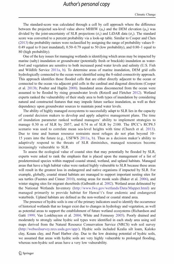
Once each of the individual vulnerability parameters were ranked (Table 1) and mapped(Fig. 2a–f), cumulative vulnerability was determined. The final spatial variation of vulnerabil-ity for each study area was found by combining the individual vulnerability parameter rastersusing a weighted geometric mean (Eq. 3).

FinalVulnerbility ¼ type2 � time2 � habitat2 � soil� inf rastructure� erosion� �1

9 ð3ÞThis approach is mathematically similar to the wetland suitability modeling methodology

used by Van Lonkhuyzen et al. (2004). Primary input parameters (type, time, and habitat) wereranked higher than secondary parameters (soil, infrastructure, and erosion) because the primaryinput parameters most directly reflect manager’s goals and objectives.

3 Results and discussion

For several reasons future sea level position is uncertain. This study uses the global meanvalues of RCP8.5 to map mid-century (0.3 by 2057) and end of the century (0.74 by 2100)impacts of SLR. We chose RCP8.5, the IPCC AR5 worst case scenario, because recent studieshave argued that sea-level could very likely exceed 1 m by the end of the century (e.g., Hortonet al. 2014; Kopp et al. 2014). Regional assessments (e.g., Slangen et al. 2012; Spada et al.2013; IPCC 2013) of SLR provide estimates for the departure of the central Pacific (Hawai‘i’slocation) from the global average. For example, by the year 2100 the tropical Pacific ispredicted to reach a sea-level value between 10 and 20% above the global mean (IPCC2013). In our study we apply global SLR rates to Hawai‘i because regional models fail to

Climatic Change

Author's personal copy

capture observed local weather patterns, local subsidence, produce inconsistencies amongprojections (Tebaldi et al. 2012), and map SLR for only one point in time (rather thanproviding a SLR curve).

With the exception of James Campbell wetland, experts expressed a moderate to very lowability to manage mid and end of the century SLR impacts according to the RCP8.5. Thegreatest gap in knowledge arose when defining long-term plans from the perspective of climatescience models and wetland experts. Wetland experts typically do not plan beyond 15 yearsinto the future due to limited staff coupled with a high number of daily responsibilities, anduncertainty in future funding. In addition much of the uncertainty in SLR projections isirreducible and stakeholders are challenged with making decisions given greater long-termuncertainty. On the other hand, current vertical uncertainty associated with LiDAR and datumerrors makes it difficult to generate accurate inundation maps using short-term SLR planningtargets (Cooper et al. 2013b). We suggest a compromise such as the rolling short-term (approx.

Fig. 2 Example vulnerability maps for Keālia National Wildlife Refuge. Vulnerability is defined and highconfidence areas (80 % probability of flooding) are mapped for six input parameters; type of inundation (a), timeof inundation (b), habitat value (c), soil type (d), infrastructure (e), and coastal erosion (f). Input parametervulnerability maps are combined (g) and areas of the highest vulnerability (red and yellow) are identified as asubset of the total area inundated at 0.74 m by 2100 (blue). High vulnerability areas are mapped at high (80%probability of flooding) and low confidence (50%)

Climatic Change

Author's personal copy

20 year) planning horizon of Donner and Webber (2014) which allows for continuous andgradual revision of policies and measures in response to the observations of impacts, newscientific findings, and improvements in SLR projections and mapping techniques. Integratingthe rolling planning horizon into the management of ‘high vulnerability’ areas may increasedecision maker’s confidence in responding to a changing climate.

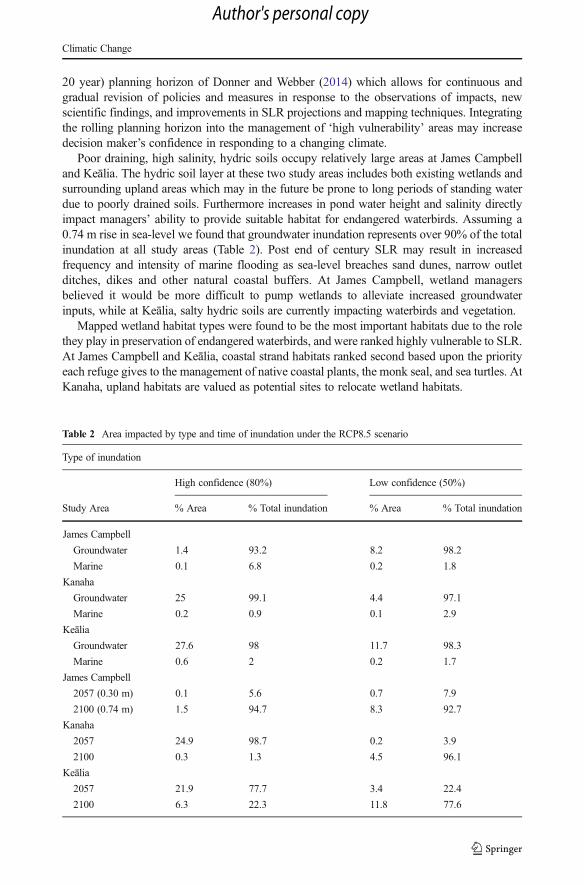
Poor draining, high salinity, hydric soils occupy relatively large areas at James Campbelland Keālia. The hydric soil layer at these two study areas includes both existing wetlands andsurrounding upland areas which may in the future be prone to long periods of standing waterdue to poorly drained soils. Furthermore increases in pond water height and salinity directlyimpact managers’ ability to provide suitable habitat for endangered waterbirds. Assuming a0.74 m rise in sea-level we found that groundwater inundation represents over 90% of the totalinundation at all study areas (Table 2). Post end of century SLR may result in increasedfrequency and intensity of marine flooding as sea-level breaches sand dunes, narrow outletditches, dikes and other natural coastal buffers. At James Campbell, wetland managersbelieved it would be more difficult to pump wetlands to alleviate increased groundwaterinputs, while at Keālia, salty hydric soils are currently impacting waterbirds and vegetation.

Mapped wetland habitat types were found to be the most important habitats due to the rolethey play in preservation of endangered waterbirds, and were ranked highly vulnerable to SLR.At James Campbell and Keālia, coastal strand habitats ranked second based upon the priorityeach refuge gives to the management of native coastal plants, the monk seal, and sea turtles. AtKanaha, upland habitats are valued as potential sites to relocate wetland habitats.

Table 2 Area impacted by type and time of inundation under the RCP8.5 scenario

Type of inundation

High confidence (80%) Low confidence (50%)

Study Area % Area % Total inundation % Area % Total inundation

James Campbell

Groundwater 1.4 93.2 8.2 98.2

Marine 0.1 6.8 0.2 1.8

Kanaha

Groundwater 25 99.1 4.4 97.1

Marine 0.2 0.9 0.1 2.9

KeāliaGroundwater 27.6 98 11.7 98.3

Marine 0.6 2 0.2 1.7

James Campbell

2057 (0.30 m) 0.1 5.6 0.7 7.9

2100 (0.74 m) 1.5 94.7 8.3 92.7

Kanaha

2057 24.9 98.7 0.2 3.9

2100 0.3 1.3 4.5 96.1

Keālia2057 21.9 77.7 3.4 22.4

2100 6.3 22.3 11.8 77.6

Climatic Change

Author's personal copy

On the basis of infrastructure alone, the areas of the highest vulnerability are located nearrefuge infrastructure or along the refuge boundaries that are bordered by community infra-structure. As the number of community infrastructure types increases there is a greater risk thatflooding within the refuge will impact bordering roads, urban, and rural communities. This isespecially true at Kanaha, which is located in downtown Kahului, Maui and is completelysurrounded by development. Accounting for land and building values in Kahului, Cooper et al.(2013a) found that a 0.75 m rise in sea-level would result in a loss of $18.7 million dollars. AtKeālia the majority of infrastructure is located on the narrow coastal strip and is bordered onboth sides by inundation.

All three study areas are currently experiencing chronic coastal erosion (Fletcher et al.2013). Two out of the three study areas have roads, houses and other developed structures thatwill prevent the natural landward migration of beaches as sea-level rises and potentially limitthe availability of coastal habitats. Coastal erosion and sea-level extreme events may beexacerbated by increased storminess and associated storm surges, however limited geograph-ical coverage of current studies and the uncertainties related to future storminess, prevents alocal assessment of impacts (IPCC 2013).

Composite vulnerability scores were compiled and the areas with the highest vulnerabilityrank were identified. At all three study areas, the dominant factor in determining vulnerabilityis whether or not an area is inundated, which is an artifact of the weighting scheme that wasapplied. Wetland managers, however, may find it useful to prioritize management efforts atflooded areas and thus the other input parameters were applied. Keālia most successfullyexemplifies the applicability of this methodology. Figure 2g illustrates both the areas predictedto be inundated by 2100 (blue) as well as a subset of the inundated areas that ranked a highervulnerability (yellow and red). Referring to our input vulnerability maps (Fig. 2a–f), the areasof highest vulnerability are defined as inundated hydric soil wetlands and the eroded coastalstrand that fall within 50 m of infrastructure. At Keālia, infrastructure serves as thedistinguishing feature in determining high vulnerability, as the majority of the flooded areaencompasses wetlands habitat and hydric soils. At Kanaha high vulnerability areas are definedas inundated wetlands, uplands and coastal stand habitats that fall within the erosion hazardzone (Online Resource 1). High vulnerability areas at James Campbell are defined as inun-dated coastal strand environments within the erosion hazard zone, and inundated wetlands withhydric soil (Online Resource 2).

4 Conclusions

Under changing climate conditions it will be increasingly difficult to achieve all conservationobjectives for habitats, species and protected areas (Hossell et al. 2003). This study is unique inthat it couples expert knowledge and empirical data to define and map input parameters thatsystematically rank SLR vulnerability. The ranking process is translated into a series of mapsthat identify ‘high vulnerability’ areas where adaptive management efforts are needed most.The entirety of this process should encourage discussion of how managing ‘high priority’ or’high vulnerability’ areas will impact current management objectives and goals. For examplecoastal decision makers should identify low lying areas and discuss how management of theseareas may be impacted by marine and groundwater sources of flooding. Creating an inventoryof infrastructure, valued habitats, and cultural assets that fall within the predicted areas offlooding may assist in prioritizing which flooded habitats to manage first.

The expert knowledge elicitation process greatly benefits from face-to-face surveys thatallow input parameters to be adequately defined or updated so that they are truly beneficial in

Climatic Change

Author's personal copy

determining rank. This process encourages decision makers to feel more confident in focusingresources to manage ‘high vulnerability’ areas. Our study employed a small sample size due tolimited management staff at each study site. Rather than consulting a larger group of expertswho may have a general idea of how each coastal ecosystem functions, wetland managersfound it more beneficial to sample a smaller number of experts who have in-depth knowledgeof site specific characteristics, historical factors, and management goals of each coastalenvironment.

The strength of this approach is that the rankings as well as the input parameters can betailored to reflect the goals and objectives of various management groups and regions. Asregional projections of SLR, storminess, and storm surge improve they can be incorporatedinto the vulnerability model to refine the designation of ‘high vulnerability’ areas. Currentlythere is much uncertainty surrounding future sea-level position. Thus, the real world adaptivechallenge is to make decisions given great long-term uncertainty. Flexible, adaptive manage-ment strategies that identify gaps in knowledge, develop alternative hypothesis, and graduallyrevise policies in response to new scientific findings and observations are necessary to producemanagement plans that openly address an uncertain future.

Acknowledgments This project was supported by the U.S. Department of Interior Pacific Islands ClimateChange Cooperative grant # 6661281, the School of Ocean Earth Science and Technology, and the NativeHawaiian Student Engineering Mentorship Program.

References

Baker JD, Littnan CL, Johnston DW (2006) Potential effects of sea level rise on the terrestrial habitats ofendangered and endemic megafauna in the Northwestern Hawaiian Islands. Endanger Species Res 2:21–30.doi:10.3354/esr002021

Bellard C, Lederc C, Courchamp F (2013) Impact of sea level rise on the 10 insular biodiversity hotspots. GlobEcol Biogeogr 23:203–212. doi:10.1111/geb.12093

Bruland GL (2008) Coastal wetlands: function and role in reducing impact of land-based management. In: FaresA, El-Kadi AI (eds) Coastal watershed management. WIT Press, Southhampton, pp 85–124

Bruun P (1962) Sea level rise as a cause of shoreline erosion. Proceedings of the American Society of CivilEngineers. J Waterways Harbors Div 88:117–130

Church JA, Clark PU, Cazenave A et al (2013) Sea level change. In: Stocker TF, Qin D, Plattner G-K, Tignor M,Allen SK, Boschung J, Nauels A, Xia Y, Bex V, Midgley PM (eds) Climate change 2013: the physicalscience basis. Contribution of working group 1 to the fifth assessment of the intergovernmental panel onclimate change. Cambridge University Press, Cambridge

Cooper H, Chen Q (2013) Incorporating uncertainty of future sea-level rise estimates into vulnerabilityassessment: a case study in Kaului, Maui. Clim Chang 121:635–647. doi:10.1007/s10584-013-0987-x

Cooper JAG, Pilkey OH (2004) Sea level rise and shoreline retreat: time to abandon the Bruun Rule. Glob PlanetChang 43:157–171. doi:10.1016/j.gloplacha.2004.07.001

Cooper H, Chen Q, Fletcher CH, Barbee MM (2013a) Assessing vulnerability due to sea-level rise in Maui,Hawaii. Clim Chang 116:547–563. doi:10.1007/s10584-012-0510-9

Cooper HM, Chen Q, Fletcher CH, Barbee M (2013b) Sea-level rise vulnerability mapping for adaptationdecisions using LiDAR DEMs. Prog Phys Geogr. doi:10.1177/0309133313496835

Donner SD, Webber S (2014) Obstacles to climate change adaptation decisions: a case study of sea-level rise andcoastal protection measures in Kiribati. Sustain Sci 9:331–345. doi:10.1007/s11625-014-0242-z

Ellison JC (2009) Wetlands of the pacific island region. Wetl Ecol Manag 17:169–206. doi:10.1007/s11273-008-9097-3

Fletcher CH, Romine BM, Genz AS, Barbee MM, Dyer M, Anderson TR, Lim SC, Vitousek S, Bochicchio C,Richmond BM (2013) National Assessment of Shoreline Change: Historical Shoreline Change in theHawaiian Islands: U.S. Geological Survey Open-File Report 2011-1051, 55 p. (http://pubs.usgs.gov/of/2011/1051)

Climatic Change

Author's personal copy

Fuentes MMPB, Cinner JE (2010) Using expert opinion to prioritize impacts of climate change on sea turtles. JEnviron Manag 9:2511–2518. doi:10.1016/j.jenvman.2010.07.013

Galbraith H, Jones R, Park R, Clough J, Herrod-Julius S, Harrington B, Page G (2002) Global climate changeand sea level rise: potential losses of intertidal habitat for shorebirds. Waterbirds 25:173–183. doi:10.1675/1524-4695(2002)025[0173:GCCASL]2.0.CO;2

Gedan KB, Kirwan ML, Wolanski E, Barbier EB, Silliman BR (2011) The present and future role of coastalwetland vegetation in protecting shorelines: answering recent challenges to the paradigm. Clim Chang 106:7–29. doi:10.1007/s10584-010-0003-7

Gesch D (2013) Consideration of vertical uncertainty in elevation-based sea-level rise assessments: Mobile Bay,Alabama case study. J Coast Res 63:197–210. doi:10.2112/SI63-016.1

Halpern BS, Selkoe KA, Fiorenza M, Kappel CV (2007) Evaluating and ranking vulnerability of global marineecosystems to anthropogenic threats. Conserv Biol 21:1301–1315. doi:10.1111/j.1523-1739.2007.00752.x

Hameed SO, Holzer KA, Doerr AN, Baty JH, Schwartz MW (2013) The value of a multi-faceted climate changevulnerability assessment to managing protected lands: Lessons from a case study in Point Reyes NationalSeashore. J Environ Manag 121:37–47. doi:10.1016/j.jenvman.2013.02.034

Hands EB (1979) Changes in rates of shore retreat, Lake Michigan, 1967–1976. Coastal Engineering ResearchCenter, Technical Memorandum No. 79–4. (71 pp.)

Horton BPS, Rahmstorf R, Engelhart SE, Kemp AC (2014) Expert assessment of sea-level rise by AD 2100 andAD 2300. Quat Sci Rev 84:1–6. doi:10.1016/j.quascirev.2013.11.002

Hossell JE, Ellis NE, Harley MJ, Hepburn IR (2003) Climate change and nature conservation: Implications forpolicy and practice in Britain and Ireland. J Nat Conserv 11:67–73. doi:10.1078/1617-1381-00034

Intergovernmental Panel on Climate Change (IPCC) (2013) Climate Change 2013 The Physical Science Basis.In: Stocker TF, Qin D, Plattner G-K, Tignor MMB, Allen SK, Boschung J, Nauels A, Xia Y, Bex V, MidgleyPM (eds), Working Group 1 Contribution to the Fifth Assessment Report of the Intergovernmental Panel onClimate Change. Available online at: http://www.climatechange2013.org/images/report/WG1AR5_Frontmatter_FINAL.pdf. Accessed 18 August, 2014

Kirwan ML, Guntenspergen GR, D’Alpaos A, Morris JT, Mudd SM, Temmerman S (2010) Limits on theadaptability of coastal marshes to rising sea level. Geophys Res Lett 37:L23401. doi:10.1029/2010GL045489

Kopp RE, Horton RM, Little CM, Mitrovica JX, Oppenhelmer M, Rasmussen DJ, Strauss BH, Tebaldi C (2014)Probabilistic 21st and 22nd century-level projections at a global network of tide-gauge sites. Earth’s Future.doi:10.1002/2014EF000239

Kuan WK, Jin G, Xin P, Robinson C, Bibbes B, Li L (2012) Tidal influence on seawater intrusion in unconfinedcoastal aquifers. Water Resour Res 48:1–11. doi:10.1029/2011WR010678

Mimura N, Nobuoka H (1995) Verification of the Bruun Rule for the estimate of shoreline retreat caused by sea-level rise. In: Dally ER, Zeidler RB (eds) Coastal dynamics 95. American Society of Civil Engineers, NewYork, pp 607–616

Mitsova D, Esnard A, Li Y (2012) Using dasymetric mapping techniques to improve the spatial accuracy of sealevel rise vulnerability assessments. J Coast Conserv 16:355–372. doi:10.1007/s11852-012-0206-3

Mora C, Frazier AG, Longman RJ et al (2013) The projected timing of climate departure from recent variability.Nature 502:183–187. doi:10.1038/nature12540

National Oceanic Atmospheric Administration (NOAA) 2010 Mapping inundation uncertainty. http://csc.noaa.gov/digitalcoast/_/pdf/ElevationMappingConfidence.pdf. Accessed 13 March 2014

Norcross ZM, Fletcher CH, Merrified M (2002) Annual and interannual changes on a reef-fringed pocket beach:Kailua Bay, Hawaii. Mar Geol 190:553–580. doi:10.1016/S0025-3227(02)00481-4

Poulter B, Haplin PN (2008) Raster modeling of coastal flooding from sea-level rise. Int J Geogr Inf Sci 22:167–182. doi:10.1080/13658810701371858

Richardson MS, Gatti RC (1999) Prioritizing wetland restoration activity within a Wisconsin watershed usingGIS modeling. J Soil Water Conserv 54:537–542

Romine BM, Fletcher CH, Barbee MM, Anderson TR, Frazier LN (2013) Are beach erosion rates and sea-levelrise related in Hawaii? Glob Planet Chang 108:149–157. doi:10.1016/j.gloplacha.2013.06.009

Rotzoll K, Fletcher CH (2012) Assessment of groundwater inundation as consequences of sea level rise. NatClim Chang 3:477–481. doi:10.1038/nclimate1725

Selkoe KA, Halpern BS, Toonen RJ (2008) Evaluating anthropogenic threats to Northwestern Hawaiian Islands.Aquat Conserv Mar Freshwat Ecosyst 18:1149–1165. doi:10.1002/aqc.961

Semlitsch RD, Bodie JR (1998) Are small, isolated wetlands expendable? Conserv Biol 12:1129–1133. doi:10.1046/j.1523-1739.1998.98166.x

Slangen ABA, Katsman CA, van de Wal RSW, Vermeersen LLA, Riva REM (2012) Towards regionalprojections of the twentyfirst century sea-level change based on IPCC SRES scenarios. Clim Dyn 38:1191–1201. doi:10.1007/s00382-011-1057-6

Climatic Change

Author's personal copy

Spada G, Bamber JL, Hurkmans RTWL (2013) The gravitationally consistent sea-level fingerprint of futureterrestrial ice lost. Geophys Res Lett 40:482–486. doi:10.1029/2012GL053000

Tebaldi C, Strauss BH, Zervas CE (2012) Modelling sea level rise impacts on storm surges along US coasts.Environ Res Lett 7:014032. doi:10.1088/1748-9326/7/1/014032

Thieler ER, Pilkey OH Jr, Young RS, Bush DM, Chai F (2000) The use of mathematical models to predict beachbehavior for US coastal engineering: a critical review. J Coast Res 16:48–70

U.S. Fish and Wildlife Service, 2011a. James Campbell National Wildlife Refuge Comprehensive ConservationPlan and Environmental Assessment. U.S. Fish and Wildlife Service, Haleiwa, Hawaii. Available fromhttp://www.fws.gov/uploadedFiles/Region_1/NWRS/Zone_1/Oahu_Complex/James_Campbell/Documents/James%20Campbell%20NWR%20CCP%20%28final%29%2012-01-11.pdf (accessed March2014)

U.S. Fish and Wildlife Service (2011b) Kealia pond national wildlife refuge comprehensive conservation planand envrionmental assessment. U.S. Fish and Wildlife Service, Kihei

Van Lonkhuyzen RA, Lagory KE, Kuiper JA (2004) Modeling the suitability of potential wetland mitigation siteswith a geographic information system. Environ Manag 33:368–375. doi:10.1007/s00267-003-3017-3

Wetzel FT, Kissling WD, Beissmann H, Penn DJ (2012) Future climate change driven sea-level rise: secondaryconsequences from human displacement for island biodiversity. Glob Chang Biol 18:2707–2719. doi:10.1111/j.1365-2486.2012.02736.x

White D, Fennessy S (2005) Modeling the suitability of wetland restoration potential at the watershed scale. EcolEng 24:359–377. doi:10.1016/j.ecoleng.2005.01.012

Zhang K, Douglas BC, Leatherman SP (2004) Global warming and coastal erosion. Clim Chang 64:41–58. doi:10.1023/B:CLIM.0000024690.32682.48

Climatic Change

Author's personal copy