SUSPENDED-SEDIMENT CONCENTRATIONS, YIELDS, TOTAL SUSPENDED SOLIDS, TURBIDITY,

AND PARTICLE-SIZE FRACTIONS FOR SELECTED RIVERS IN MINNESOTA, 2007 THROUGH 2011

Christopher A. Ellison, Hydrologist, USGS, cellison@usgs.gov, 763.783.3121

Brett E. Savage, Hydrologic Technician, USGS, besavage@usgs.gov, 763.783.3133

Gregory D. Johnson, Senior Hydrologist, MPCA, gregory.johnson@state.mn.us, 651.757.2471

Abstract

Excessive sediment transport in rivers causes problems for flood control, soil conservation, irrigation, aquatic health,

and navigation, as well as transporting harmful contaminants like organic chemicals and eutrophication-causing

nutrients. In Minnesota, more than 5,800 miles of streams are identified as impaired by the Minnesota Pollution

Control Agency (MPCA) due to elevated levels of suspended sediment.

The U.S. Geological Survey, in cooperation with the MPCA, established a sediment monitoring network in 2007

and began systematic sampling of suspended-sediment concentration (SSC), total suspended solids (TSS), and

turbidity in rivers across Minnesota to improve the understanding of fluvial sediment transport relations. Suspended-

sediment samples were collected from 14 sites from 2007 through 2011. Analyses of these data indicated that the

Zumbro River at Kellogg in southeast Minnesota had the highest mean SSC of 226 milligrams per liter (mg/L)

followed by the Minnesota River at Mankato with a mean SSC of 193 mg/L. The single highest SSC of 1,250 mg/L

was measured at the Zumbro River during the 2011 spring runoff. The lowest mean SSC of 21 mg/L was measured

at Rice Creek in the northern Minneapolis-St. Paul metropolitan area.

Total suspended solids (TSS) have been used as a measure of fluvial sediment by the MPCA since the early 1970s;

however, TSS concentrations have been known to underrepresent the amount of suspended sediment. For this study,

comparisons between concurrently sampled SSC and TSS indicated significant differences at every site, with SSC

on average two times larger than TSS concentrations.

Regression analysis indicated that 7 out of 14 sites had poor or no relation between SSC and streamflow. Only two

sites, the Knife River and the Wild Rice River at Twin Valley, had strong correlations between SSC and streamflow,

with coefficient of determination (R2) values of 0.82 and 0.80, respectively. In contrast, turbidity had moderate to

strong relations with SSC at 10 of 14 sites and was superior to streamflow for estimating SSC at all sites.

Suspended-sediment basin yields indicated that the Minnesota River had the largest mean annual sediment basin

yield of 120 tons of sediment per year per square mile.

INTRODUCTION

Excessive sediment transported in rivers causes problems for flood control, soil conservation, irrigation, aquatic

health, and navigation. Fluvial sediment becomes entrained in a stream by way of erosion from land surfaces, or

from channel bed and bank erosion. Streams transport sediment by maintaining the finer particles in suspension with

turbulent currents (suspended-sediment load) and by intermittent entrainment and movement of coarser particles

along the streambed (bedload). Fine-grained sediment can serve to transport harmful contaminants such as organic

chemicals, heavy metals, and eutrophication-causing nutrients (Baker, 1980).

The most recent U.S. Environmental Protection Agency compilation of States’ water-quality reports under Section

305(b) of the Clean Water Act identifies sediment as one of the leading causes of impairment in the Nation’s rivers

and streams (U.S. Environmental Protection Agency, 2009, 2012). In Minnesota, more than 5,800 miles of streams

are identified as impaired due to elevated levels of suspended sediments (Minnesota Pollution Control Agency,

2009a).

The Minnesota Pollution Control Agency (MPCA) incorporated a grab sampling procedure and laboratory analysis

of total suspended solids (TSS) for measurement of fluvial sediment in the early 1970s. The grab sampling

procedure and TSS measure were adopted by the MPCA for various reasons, including the assumption that the TSS

method would provide an adequate representation of suspended sediment and the procedures for the collection and

laboratory analysis of samples for suspended-sediment concentration were cost prohibitive. Marked differences

between TSS and SSC field sampling procedures and subsequent laboratory analysis largely contribute to the

significant differences between concentrations of TSS and SSC (Gray et. al, 2000). For field sampling, TSS samples

are collected at the center of the stream cross section (Minnesota Pollution Control Agency, 2011), whereas SSC

samples are collected using federally approved (through the Federal Interagency Sedimentation Project) isokinetic

samplers (Davis, 2005) and width- and depth-integrated procedures as described by Edwards and Glyssen (1999).

The primary difference in laboratory procedures is that the TSS analytical method uses a pipette to extract a

predetermined volume (subsample) from the original water sample to determine the amount of suspended material,

whereas the SSC analytical method measures all of the sediment and the mass of the entire water-sediment mixture

(American Public Health Association, American Water Works Association, and Water Pollution Control Federation,

1998). Gray et. al (2000) reported that the use of a pipette to obtain subsamples subjects the analyses to substantial

biases compared to the SSC method.

The continued need to measure fluvial sediment and recent technological advances has led to the use of turbidity as

a surrogate for suspended sediment, particularly in locations where streamflow alone is not a good estimator of SSC

(Lewis, 1996; Rasmussen et. al, 2009). Optical turbidity sensors measure the amount of emitted light that is reflected

by suspended particles in the water column, and have been used successfully to predict SSC, assuming the relation

between the turbidity signal and SSC can be calibrated from physical samples (Lewis, 1996; Christensen et. al,

2000; Uhrich and Bragg, 2003; Rasmussen et. al, 2009). For this study, a portable desktop turbidity meter was used

to measure turbidity concurrently with SSC sampling to investigate what relation may exist between turbidity and

SSC for streams in Minnesota.

The purpose of the study presented here was to document findings based on sediment data collected by the U.S.

Geological Survey (USGS), in cooperation with the MPCA, on selected rivers in Minnesota from 2007 through

2011. Specifically, the study examines suspended-sediment data to (1) describe suspended-sediment concentrations

(SSC), total suspended solids (TSS), turbidity, and particle-size fractions for selected rivers across Minnesota’s

major watersheds; (2) quantify the difference between SSC and TSS; (3) develop relations among streamflow, SSC,

TSS, turbidity, and suspended-sediment loads; and (4) estimate suspended-sediment loads and basin yields. This

paper presents a condensation of the study by Ellison et. al (2014) and associated results.

DESCRIPTION OF THE STUDY AREA

A map of the State showing the locations of the sites in this study relative to the major watersheds and major streams

in Minnesota is shown in Figure 1.

Figure 1 Major watersheds and locations of sediment sampling sites in Minnesota.

The 10 watersheds selected for this study represent a cross section of watershed characteristics present in Minnesota.

Minnesota’s geologic history of advancing and retreating glaciers affected most of the State and contributed to the

development of the general soil types and topographic relief (Sims and Morey, 1972). Most of the northeastern part

of the State is forested, but has some open pasture and sparse cultivated crops (Tornes, 1986). The far western and

southern regions of Minnesota are intensively cultivated. Between these regions lies a transition area with a mixture

of cultivated crops, pasture, and forests. Urban (developed) areas are scattered throughout the State, but the largest is

the Minneapolis-St. Paul metropolitan area.

METHODS OF DATA COLLECTION AND ANALYSIS

Data were collected from February 2007 through November 2011. Fourteen sites were sampled 5–14 times per year

during the open-water season (Table 1). Few samples were collected during the winter months because historically,

less than 4 percent of annual loads were transported during the winter months (Tornes, 1986). Water samples were

collected at all sites for analysis of SSC and particle-size fractions less than 0.0625 millimeters (mm) (fines). For

this study, particles in suspension greater than 0.0625 mm are categorized as sands.

Table 1 Sediment sampling stations in selected watersheds in Minnesota, 2007 through 2011.

[USGS, U.S. Geological Survey; NAD 83, North American Datum of 1983; mi2, square miles]

Site

number

(Figure 1)

USGS

station

number

Station name

Latitude

(north)

(NAD 83)

Longitude

(west)

(NAD 83)

Drainage

area

(mi2)

Number of

suspended-

sediment

samples

1 04015330 Knife River near Two

Harbors, Minn.

46° 56' 49" 91° 47' 32" 84 27

2 05061500 South Branch Buffalo

River at Sabin, Minn.

46° 46' 32" 96° 37' 40" 454 40

3 05062500 Wild Rice River at Twin

Valley, Minn.

47° 16' 00" 96° 14' 40" 934 29

4 05063000 Wild Rice River near Ada,

Minn.

47° 15' 50" 96° 30' 00" 1,100 29

5 05063340 South Branch Wild Rice

River near Ulen, Minn.

47° 05' 17" 96° 15' 31" 141 25

6 05063400 South Branch Wild Rice

River near Felton, Minn.

47° 07' 23" 96° 24' 25" 180 28

7 05064000 Wild Rice River at

Hendrum, Minn.

47° 16' 05" 96° 47' 50" 1,560 27

8 05131500 Little Fork River at

Littlefork, Minn.

48° 23' 45" 93° 32' 57" 1,680 34

9 05278930 Buffalo Creek near

Glencoe, Minn.

44° 45' 50" 94° 05' 27" 373 44

10 05288580 Rice Creek below Old

Hwy. 8 in Mounds View,

Minn.

45° 05' 36" 93° 11' 42" 156 21

11 05320270 Little Cobb River near

Beauford, Minn.

43° 59' 48" 93° 54' 30" 130 68

12 05325000 Minnesota River at

Mankato, Minn.

44° 10' 08" 94° 00' 11" 14,900 32

13 05374900 Zumbro River at Kellogg,

Minn.

44° 18' 43" 92° 00' 14" 1,400 34

14 05476000 Des Moines River at

Jackson, Minn.

43° 37' 06" 94° 59' 05" 1,250 25

Streamflow data were obtained from existing USGS or MPCA/Minnesota Department of Natural Resources

(MDNR) streamgages. Of the 14 sampling sites, 13 were colocated at the corresponding streamgage; the exception

was the South Branch Wild Rice River near Ulen (site 5) where no streamgage was available. For the South Branch

Wild Rice River near Ulen (site 5), streamflow was estimated by extending streamflow from a nearby USGS

streamgage [South Branch Wild Rice River near Felton (site 6)] using the MOVE-1 (Maintenance of Variance

Extension, Type 1) statistical program (Hirsch, 1982).

DATA COLLECTION

Suspended-sediment samples were collected at all 14 sites using isokinetic samplers and equal width and depth-

integrating techniques following procedures by Edwards and Glysson (1999). Most samples were collected using a

D–74 rigid bottle sampler suspended from a bridge during nonwadeable flows and a DH–48 hand-held sampler

during wadeable flows. Following collection, samples were transported to the USGS sediment laboratory in Iowa

City, Iowa, where they were composited into a single sample and analyzed for suspended-sediment concentration

and fines particle-size fraction.

Grab samples for laboratory TSS analysis were collected in 1-liter (L) plastic containers near the centroid of the

stream cross section following MPCA sampling protocols (Minnesota Pollution Control Agency, 2011). The TSS

samples were collected at seven sites and were refrigerated and delivered to the Minnesota Department of Health

laboratory in St. Paul, within seven days of the collection date.

Grab samples for field measurements of turbidity were collected at 13 of 14 sites (Minnesota River at Mankato were

only collected periodically) from the centroid of the stream cross section in a 1-L plastic container. A subsample of

the contents was transferred into a glass vial, which was then placed into the instrument cell compartment of a

portable Hach model 2100P (Hach Company, Loveland, Colorado) turbidimeter to obtain the measurement.

Daily mean streamflow data were obtained from existing USGS or MPCA/MDNR streamgages to develop sediment

transport relations and to calculate sediment loads. Streamflow data for 10 of the sites were from the USGS

(http://waterdata.usgs.gov/mn/nwis/sw/), and streamflow data for 3 sites (sites 4, 9, and 13; Table 1) were from the

MPCA (http://www.dnr.state.mn.us/waters/csg/index.html). The USGS and MPCA/MDNR determine streamflow at

streamgages by use of the rating-curve method (the relation between streamgage height and streamflow) for each

station following Rantz et. al (1982).

DATA ANALYSIS

Sediment concentration data and measures of daily mean streamflow were analyzed to obtain summary statistics and

perform nonparametric match-pair tests, simple linear regression (SLR), and load estimation using S-Plus statistical

analysis software (TIBCO Software Inc., 2010). The Wilcoxon signed-rank test (Helsel and Hirsch, 2002) was

conducted to determine if significant differences could be detected between matched pairs of SSC and TSS.

For model development, SLR was used to calculate SSC based on daily mean streamflow, TSS, and turbidity. For

SLR models, p-values were used to evaluate the model’s null hypothesis for statistical significance [p-values less

than (<) 0.05 indicated statistical significance], whereas the coefficient of determination (R2) was used to assess the

linear association between the response and explanatory variable and to assess how well the model was able to

accurately predict outcomes of the response variable.

The SLR can be used to estimate unknown values of a response variable from a known quantity of an explanatory

variable if a statistically significant correlation between the variables exists. For SLR to produce a useable model,

assumptions are that the two variables are related linearly, that the variance of the residuals is constant

(homoscedastic), and that the residuals are distributed normally (Helsel and Hirsch, 2002). These assumptions

commonly are violated by measured water data, so the data are transformed to logarithmic values to satisfy these

assumptions. Logarithmic base-10 (log10) transformation has been determined to be effective in normalizing

residuals for many water-quality measures and streamflow (Helsel and Hirsch, 2002). There exists a consequence of

transformation of the response variable, in this case SSC, which must be accounted for when computing SSC values.

When the regression estimates are retransformed to the original units, bias is introduced (usually negative) in the

computed SSC values (Miller, 1951; Koch and Smillie, 1986). To correct for this retransformation bias, Duan

(1983) introduced a nonparametric bias-correction factor (BCF) called the “smearing” estimator. The equation to

compute the smearing BCF for base-10 logarithmic transformation follows (Duan, 1983):

𝐵𝐶𝐹 = (∑ 10𝑒𝑖)/𝑛𝑛

𝑖=1 (1)

where

n is the number of samples, and

ei is the difference between each measured and estimated concentration, in log units.

Regression-computed SSC values are corrected for bias by multiplying the retransformed SSC value by the BCF.

Sediment loads were estimated using S-LOADEST, which is an interface-driven, S-PLUS version of LOADEST,

which is a FORTRAN program for estimating constituent loads in streams and rivers (Runkel et. al, 2004). The S-

LOADEST program is based on a rating-curve method (Cohn et. al, 1989, 1992; Crawford, 1991) that uses

regression to estimate constituent loads in relation to several explanatory variables, which most commonly are

streamflow and time (seasonal component). The regression is developed using daily loads calculated from the

sample concentration and daily flow for that sample.

SUSPENDED-SEDIMENT CONCENTRATIONS, TOTAL SUSPENDED SOLIDS, TURBIDITY, AND

PARTICLE-SIZE FRACTIONS

Sediment samples were collected during a wide variety of streamflow conditions. The Zumbro River at Kellogg (site

13) had the highest mean SSC [226 milligrams per liter (mg/L)] among all sites. High SSC in the Zumbro River is

attributed in part to the combined effects of climate, high topographic relief, and erodible soils. Steep terrain in the

lower part of the watershed increases the erosion potential. The Minnesota River at Mankato (site 12) also had high

mean SSC (193 mg/L). Although the Minnesota River Valley has low relief in the valley, the edges of the river

valley are lined with steep bluffs and ravines (Minnesota Pollution Control Agency, 2009b). The Zumbro River at

Kellogg produced the single highest SSC of 1,250 mg/L at a streamflow of 1,800 cubic feet per second (ft3/s) during

the 2011 spring snowmelt runoff. The Wild Rice River near Ada (site 4) had a mean SSC of 185 mg/L, similar in

magnitude to the Minnesota River. Elevated SSC values on the main stem of the Wild Rice River have been linked

to cultivated agriculture (Brigham et. al, 2001) and artificial channelization of the main stem from flood-control

projects. One of the lowest mean SSC values of 37 mg/L occurred within the same watershed at the South Branch

Wild Rice River near Ulen (site 5). The lowest mean SSC of 21 mg/L occurred at Rice Creek below Old Highway 8

in Mounds View (site 10) in the northern Minneapolis-St. Paul metropolitan area. The lowest SSC values of 2 mg/L

were measured at the Little Cobb River near Beauford (site 11) on December 28, 2010, at a streamflow of 108 ft3/s;

at Rice Creek on September 15, 2010, at a streamflow of 31 ft3/s; and at the Knife River near Two Harbors (site 1)

on September 10, 2008, at a streamflow of 5 ft3/s.

The TSS samples were collected concurrently with SSC samples at seven sites, and TSS concentrations followed

similar spatial patterns as SSC. For example, similar to the SSC data, the largest mean TSS concentration of 182

mg/L was measured at the Zumbro River, whereas the smallest mean TSS of 25 mg/L was measured at the Little

Fork River at Littlefork (site 8).

Variability in turbidity measurements was relatively smaller than SSC variability and followed spatial patterns

similar to those of SSC and TSS. The Zumbro River and Wild Rice River near Ada had the largest mean turbidity

values of 101 and 89 nephelometric turbidity ratio units (NTRUs), respectively. Rice Creek had the smallest single

turbidity value along with a very narrow range of values (1 to 9 NTRUs). The narrow range of values observed at

Rice Creek is attributed to the combined effect of low SSC and high percentage of sand-sized particles. Laboratory

trials indicate that turbidity sensors are less sensitive to sand-sized particles than to fine-sized particles (Conner and

De Visser, 1992; Hatcher et. al, 2000).

For particle sizes, suspended fines (sediment sizes less than 0.0625 mm) were documented in markedly higher

percentages than suspended sands at all sites, with the exception of Rice Creek. The largest mean percentage of fines

was at the Wild Rice River at Hendrum (site 7), where 92 percent of the material in suspension consisted of fines.

Other large mean percentages of fines were at the South Branch Buffalo River at Sabin (site 2), Wild Rice River at

Twin Valley (site 3), and the Little Fork River with 88, 83, and 84 percent, respectively. Suspended fines were

noticeably lower at Rice Creek when compared to other sites. Although fine-sized particles composed most of the

total suspended sediment, the percentage of suspended sands was appreciable for many samples at many sites. The

largest mean percentage of sand particles in suspension was observed at Rice Creek, where a mean of 45 percent of

the material in suspension was sand-sized. Other substantial mean percentages of sands were measured at the

Zumbro River, South Branch Wild Rice River near Felton (site 6), and the Minnesota River with 35, 33, and 28

percent, respectively.

COMPARISON BETWEEN SUSPENDED-SEDIMENT CONCENTRATIONS AND TOTAL SUSPENDED

SOLIDS

For this analysis, the Wilcoxon signed-rank test (Helsel and Hirsch, 2002) was used to test if concurrently sampled

pairs of SSC and TSS were different within sites. Box plots illustrate the variation in SSC and TSS at all sites

(Figure 2) and are consistent with the Wilcoxon signed-rank test results, which indicated median values of SSC were

larger than median values of TSS at each of the seven sites where TSS samples were collected concurrently with

SSC. When comparing SSC to TSS median concentrations, the overall mean percent difference indicated that SSC

was about 100 percent larger than TSS. The largest percent difference between median values of SSC and TSS was

at the South Branch Buffalo River site and the smallest difference was at the Des Moines River.

Figure 2 Boxplots of suspended-sediment concentrations (SSC) and total suspended solids (TSS) for selected sites in

Minnesota, 2007 through 2011.

RELATIONS AMONG STREAMFLOW, SUSPENDED-SEDIMENT CONCENTRATIONS, TOTAL

SUSPENDED SOLIDS, AND TURBIDITY

Variations in streamflow provide important information related to the timing and changes in sediment

concentrations and has widely been used to develop SSC prediction models. The relation between SSC and

streamflow for each site is presented in Table 2 and illustrated in Figure 3. Best-fit regression lines represent the

relation between SSC and streamflow, and can be used to evaluate how SSC responds to changes in streamflow

within and among sites. The gradient of the lines provides an indication of how quickly SSC changes with changes

in streamflow. The strength of the relation can be seen in how closely the observed data fall along the regression

line. Lines with steep positive gradients from left to right indicate SSC increases quickly as streamflow increases. In

this study, the sites with the steepest gradients were the Knife River, Wild Rice River near Twin Valley, Wild Rice

River near Ada, Little Fork River, Rice Creek, Minnesota River, and Zumbro River (Figure 3). Moderate gradients

were observed at the South Branch Wild Rice River near Felton and the Des Moines River. Low or level gradients,

which indicate that SSC changes little as streamflow increases, were observed at the South Branch Wild Rice River

near Ulen, Buffalo Creek, and the Little Cobb River. The negative relation, indicated by a negative gradient, for the

South Branch Buffalo River, is unusual. Negative gradients indicate that the amount of suspended sediment in

streams may be diluted during periods of increased streamflow due to limited supply of sediment.

Table 2 Summary of simple linear regression models to evaluate suspended-sediment concentrations using

streamflow as the explanatory variable for selected sites in Minnesota, 2007 through 2011.

[mg/L, milligrams per liter; R2, coefficient of determination; BCF, Duan’s bias correction factor; SSC, suspended-

sediment concentration; Q, daily mean streamflow; <, less than]

Site

number

(Figure 1)

Station name

Number of

samples

used for

regression

Regression model

(mg/L) R2

Standard

error

residual

(mg/L)

p-value BCF

1 Knife River near Two Harbors,

Minn.

27 SSC = 0.9276×Q0.7175 0.82 12.7 <0.01 1.227

2 South Branch Buffalo River at

Sabin, Minn.

40 SSC = 280.7×Q-0.2213 0.22 10.7 <0.01 1.270

3 Wild Rice River at Twin

Valley, Minn.

29 SSC = 0.2691×Q0.9241 0.80 25.8 <0.01 1.212

4 Wild Rice River near Ada,

Minn.

29 SSC = 0.5526×Q0.8579 0.67 34.0 <0.01 1.417

5 South Branch Wild Rice River

near Ulen, Minn.

25 SSC = 26.1×Q0.0987 0.00 6.2 0.34 1.423

6 South Branch Wild Rice River

near Felton, Minn.

27 SSC = 20.93×Q0.3085 0.14 26.1 0.03 1.643

7 Wild Rice River at Hendrum,

Minn.

27 SSC = 24.84×Q0.2163 0.16 17.0 0.02 1.284

8 Little Fork River at Littlefork,

Minn.

32 SSC = 1.360×Q0.4563 0.65 3.8 <0.01 1.119

9 Buffalo Creek near Glencoe,

Minn.

42 SSC = 43.2×Q0.0897 0.02 10.2 0.19 1.581

10 Rice Creek below Old Hwy. 8

in Mounds View, Minn.

21 SSC = 0.2842×Q0.9223 0.44 3.1 <0.01 1.263

11 Little Cobb River near

Beauford, Minn.

68 SSC = 102×Q0.0003 0.02 8.2 0.99 1.310

12 Minnesota River at Mankato,

Minn.

32 SSC = 9.738×Q0.3286 0.41 20.0 <0.01 1.173

13 Zumbro River at Kellogg,

Minn.

18 SSC = 0.0348×Q1.2314 0.54 61.5 <0.01 1.399

14 Des Moines River at Jackson,

Minn.

25 SSC = 23.07×Q0.2419 0.17 15.6 0.02 1.313

Results of the SLR analysis between SSC and streamflow presented in Table 2 provide a quantitative description of

the plots shown in Figure 3. The relation between SSC and streamflow was significant statistically (p-value <0.05)

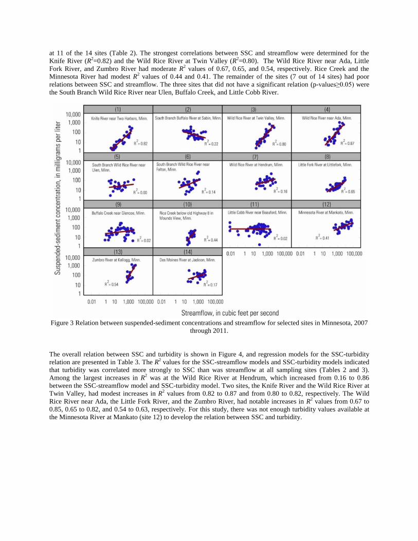
at 11 of the 14 sites (Table 2). The strongest correlations between SSC and streamflow were determined for the

Knife River (R2=0.82) and the Wild Rice River at Twin Valley (R

2=0.80). The Wild Rice River near Ada, Little

Fork River, and Zumbro River had moderate R2 values of 0.67, 0.65, and 0.54, respectively. Rice Creek and the

Minnesota River had modest R2 values of 0.44 and 0.41. The remainder of the sites (7 out of 14 sites) had poor

relations between SSC and streamflow. The three sites that did not have a significant relation (p-values≥0.05) were

the South Branch Wild Rice River near Ulen, Buffalo Creek, and Little Cobb River.

Figure 3 Relation between suspended-sediment concentrations and streamflow for selected sites in Minnesota, 2007

through 2011.

The overall relation between SSC and turbidity is shown in Figure 4, and regression models for the SSC-turbidity

relation are presented in Table 3. The R2 values for the SSC-streamflow models and SSC-turbidity models indicated

that turbidity was correlated more strongly to SSC than was streamflow at all sampling sites (Tables 2 and 3).

Among the largest increases in R2 was at the Wild Rice River at Hendrum, which increased from 0.16 to 0.86

between the SSC-streamflow model and SSC-turbidity model. Two sites, the Knife River and the Wild Rice River at

Twin Valley, had modest increases in R2 values from 0.82 to 0.87 and from 0.80 to 0.82, respectively. The Wild

Rice River near Ada, the Little Fork River, and the Zumbro River, had notable increases in R2 values from 0.67 to

0.85, 0.65 to 0.82, and 0.54 to 0.63, respectively. For this study, there was not enough turbidity values available at

the Minnesota River at Mankato (site 12) to develop the relation between SSC and turbidity.

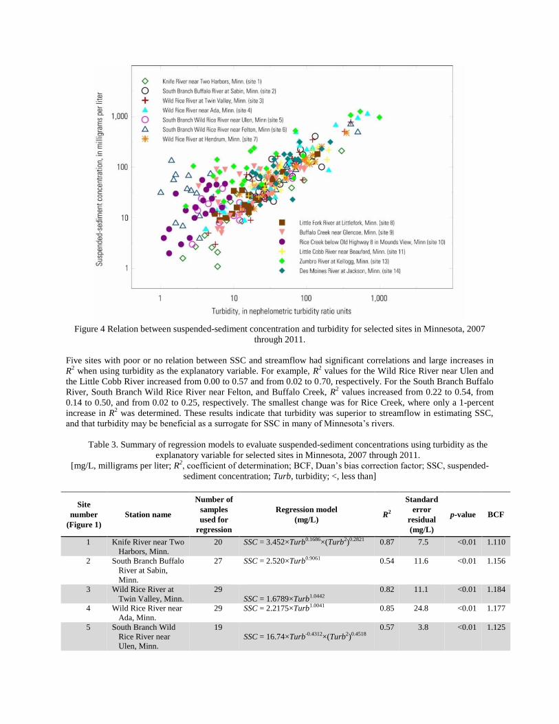
Figure 4 Relation between suspended-sediment concentration and turbidity for selected sites in Minnesota, 2007

through 2011.

Five sites with poor or no relation between SSC and streamflow had significant correlations and large increases in

R2 when using turbidity as the explanatory variable. For example, R

2 values for the Wild Rice River near Ulen and

the Little Cobb River increased from 0.00 to 0.57 and from 0.02 to 0.70, respectively. For the South Branch Buffalo

River, South Branch Wild Rice River near Felton, and Buffalo Creek, R2 values increased from 0.22 to 0.54, from

0.14 to 0.50, and from 0.02 to 0.25, respectively. The smallest change was for Rice Creek, where only a 1-percent

increase in R2 was determined. These results indicate that turbidity was superior to streamflow in estimating SSC,

and that turbidity may be beneficial as a surrogate for SSC in many of Minnesota’s rivers.

Table 3. Summary of regression models to evaluate suspended-sediment concentrations using turbidity as the

explanatory variable for selected sites in Minnesota, 2007 through 2011.

[mg/L, milligrams per liter; R2, coefficient of determination; BCF, Duan’s bias correction factor; SSC, suspended-

sediment concentration; Turb, turbidity; <, less than]

Site

number

(Figure 1)

Station name

Number of

samples

used for

regression

Regression model

(mg/L) R2

Standard

error

residual

(mg/L)

p-value BCF

1 Knife River near Two

Harbors, Minn.

20 SSC = 3.452×Turb0.1686×(Turb2)0.2821 0.87 7.5 <0.01 1.110

2 South Branch Buffalo

River at Sabin,

Minn.

27 SSC = 2.520×Turb0.9061 0.54 11.6 <0.01 1.156

3 Wild Rice River at

Twin Valley, Minn.

29

SSC = 1.6789×Turb1.0442

0.82 11.1 <0.01 1.184

4 Wild Rice River near

Ada, Minn.

29 SSC = 2.2175×Turb1.0041 0.85 24.8 <0.01 1.177

5 South Branch Wild

Rice River near

Ulen, Minn.

19

SSC = 16.74×Turb-0.4312×(Turb2)0.4518

0.57 3.8 <0.01 1.125

6 South Branch Wild

Rice River near

Felton, Minn.

26

SSC = 50.37×Turb-0.531×(Turb2)0.3827

0.50 25.3 <0.01 1.319

7 Wild Rice River at

Hendrum, Minn.

26

SSC = 2.261×Turb0.8979

0.86 12.9 <0.01 1.043

8 Little Fork River at

Littlefork, Minn.

23 SSC = 1.784×Turb 0.9428 0.82 1.7 <0.01 1.056

9 Buffalo Creek near

Glencoe, Minn.

27 SSC = 10.43×Turb 0.5468 0.25 6.1 <0.01 1.383

10 Rice Creek below

Old Hwy 8. in

Mounds View,

Minn.

20 SSC = 3.487Turb 2.022 0.45 15.5 <0.01 1.266

11 Little Cobb River

near Beauford,

Minn.

23 SSC = 4.765×Turb 0.7351 0.70 7.0 <0.01 1.067

13 Zumbro River at

Kellogg, Minn.

24 SSC = 23.19×Turb 0.6105 0.63 37.4 <0.01 1.261

14 Des Moines River at

Jackson, Minn.

21 SSC = 4.751×Turb 0.8088 0.38 11.3 <0.01 1.164

SUSPENDED-SEDIMENT BASIN YIELDS

Suspended-sediment loads were calculated to estimate basin yields using the S-LOADEST program. The S-

LOADEST program incorporates time-series data for streamflow, a dataset of constituent concentrations, and a time

component to estimate annual and seasonal loads for the constituent of interest. The form of the regression equation

used in the S-LOADEST model is described in Ellison et. al (2014). Mean annual basin yields for suspended

sediment, suspended sands, and suspended fines are shown in Figure 5. Comparing annual sediment yields among

sites across Hydrologic Unit Code Level 4 watersheds provides insight on erosion rates and describes the relative

measure of degradation occurring on the landscape.

Figure 5 Mean annual basin yields of suspended sediment for selected sites in Minnesota, 2007 through 2011.

ACKNOWLEDGMENTS

This report presents a compilation of information supplied by many agencies and individuals. The authors would

like to thank the Minnesota Pollution Control Agency, Wild Rice Watershed District, and the Rice Creek Watershed

District for their assistance with this study. Dave Lorenz, Kristen Kieta, Joel Groten, Domenic Murino, Lance

Ostiguy, Mark Brigham, and Christiana Czuba of the U.S. Geological Survey are acknowledged for assistance with

office and field aspects of the study. Any use of trade, firm, or product names is for descriptive purposes only and

does not imply endorsement by the U.S. Government.

REFERENCES

American Public Health Association, American Water Works Association, and Water Pollution Control Federation.

(1998). Standard methods for the examination of water and wastewater (20th ed.): Washington, D.C., American

Public Health Association, American Water Works Association, Water Environment Federation, [variously paged].

Baker, R.A. (1980). Contaminants and sediment—Volume 1, Fate and transport, case studies, modeling, toxicity: Ann

Arbor, Mich., Ann Arbor Science, 558 p.

Brigham, M.E., McCullough, C.J., and Wilkinson, P. (2001). Analysis of suspended-sediment concentrations and

radioisotope levels in the Wild Rice River Basin, northwestern Minnesota, 1973–98: U.S. Geological Survey Water-

Resources Investigations Report 01–4192, 21 p.

Christensen, V.G., Jian, Xiaodong, and Ziegler, A.C. (2000). Regression analysis and real-time water-quality monitoring

to estimate constituent concentrations, loads, and yields in the Little Arkansas River, south-central Kansas, 1995–99:

U.S. Geological Survey Water-Resources Investigations Report 00–4126, 36 p. (Available at

http://pubs.er.usgs.gov/publication/wri004126.)

Cohn, T.A., Delong, L.L., Gilroy, E.J., Hirsch, R.M., and Wells, D.K. (1989). Estimating constituent loads: Water

Resources Research, v. 25, no. 5, p. 937–942. (Available at http://dx.doi.org/10.1029/WR025i005p00937.)

Cohn, T.A., Caulder, D.L., Gilroy, E.J., Zynjuk, L.D., and Summers, R.M.. (1992). The validity of a simple statistical

model for estimating fluvial constituent loads—An empirical study involving nutrient loads entering Chesapeake

Bay: Water Resources Research, v. 28, no. 9, p. 2,353–2,363. (Available at http://dx.doi.org/10.1029/92WR01008.)

Conner, C.S., and De Visser, A.M. (1992). A laboratory investigation of particle size effects on an optical backscatterance

sensor: Marine Geology, v. 108, no. 2, p. 151–159. (Available at http://dx.doi.org/10.1016/0025-3227(92)90169-I.)

Crawford, C.G. (1991). Estimation of suspended-sediment rating curves and mean suspended-sediment loads: Journal of

Hydrology, v. 129, p. 331–348. (Available at http://dx.doi.org/10.1016/0022-1694(91)90057-O.)

Davis, B.E. (2005). A guide to the proper selection and use of federally approved sediment and water-quality samplers:

U.S. Geological Survey Open-File Report 2005–1087, 20 p. (Available at http://pubs.usgs.gov/of/2005/1087/.)

Duan, N. (1983). Smearing estimate—A nonparametric retransformation method: Journal of the American Statistical

Association, v. 78, no. 383, p. 605–610. (Available at http://dx.doi.org/10.1080/01621459.1983.10478017.)

Edwards, T.K., and Glysson, G.D. (1999). Field methods for measurement of fluvial sediment: U.S. Geological Survey

Techniques of Water-Resources Investigations, book 3, chap. C2, 89 p. (Available at

http://pubs.usgs.gov/twri/twri3-c2/.)

Ellison, C.A., Savage, B.E., and Johnson, G.D. (2014). Suspended-sediment concentrations, loads, total suspended solids,

turbidity, and particle-size fractions for selected rivers in Minnesota, 2007 through 2011: U.S. Geological Survey

Scientific Investigations Report 2013–5205, 43 p., http://dx.doi.org/10.3133/sir20135205.

Gray, J.R., Glysson, G.D., Turcios, L.M., and Schwarz, G.E. (2000). Comparability of suspended-sediment concentration

and total suspended solids data: U.S. Geological Survey Water-Resources Investigations Report 00–4191, 14 p.

(Available at http://pubs.usgs.gov/wri/wri004191/.)

Hatcher, Annamarie, Hill, P.S., Grant, Jon, and Macpherson, P. (2000). Spectral optical backscatter of sand suspension—

Effects of particle size, composition and color: Marine Geology, v. 168, p. 115–128 (Available at

http://dx.doi.org/10.1016/S0025-3227(00)00042-6.)

Helsel, D.R., and Hirsch, R.M. (2002). Statistical methods in water resources—Hydrologic analysis and interpretation:

U.S. Geological Survey Techniques of Water-Resources Investigations, book 4, chap. A3, 510 p., (Available at

http://pubs.usgs.gov/twri/twri4a3/.)

Hirsch, R.M. (1982). A comparison of four streamflow record extension techniques: Water Resources Research, v. 18, no.

4, p. 1,081–1,088. (Available at http://dx.doi.org/10.1029/WR018i004p01081.)

Koch, R.W., and Smillie, G.M. (1986). Bias in hydrologic prediction using log-transformed regression models: Journal of

the American Water Resources Association, v. 22, no. 5, p. 717–723. (Available at http://dx.doi.org/10.1111/j.1752-

1688.1986.tb00744.x.)

Lewis, J. (1996). Turbidity controlled suspended sediment sampling for runoff event load estimation: Water Resources

Research, v. 32, no. 7, p. 2,299–2,310. (Available at http://dx.doi.org/10.1029/96WR00991.)

Miller, C.R. (1951). Analysis of flow-duration sediment rating curve method of computing sediment yield: U.S.

Department of Interior, Bureau of Reclamation, 55 p.

Minnesota Pollution Control Agency. (2009a). Minnesota’s impaired waters and total maximum daily loads (TMDLs):

accessed December 12, 2012, at http://www.pca.state.mn.us/water/tmdl/index.html.

Minnesota Pollution Control Agency. (2009b). Identifying sediment sources in the Minnesota River Basin: accessed

January 9, 2013, at http://www.pca.state.mn.us/index.php/view-document.html?gid=8099.

Minnesota Pollution Control Agency. (2011). Standard operating procedures (SOP) intensive watershed monitoring—

Stream water quality component: accessed August 2, 2012, at http://www.pca.state.mn.us/index.php/view-

document.html?gid=16141.

Rantz, S.E., and others. (1982). Measurement and computation of streamflow—Volume 1, Measurement of stage and

discharge, and volume 2, Computation of discharge: U.S. Geological Survey Water-Supply Paper 2175, 631 p.

(Available at http://pubs.usgs.gov/wsp/wsp2175/.)

Rasmussen, P.P., Gray, J.R., Glysson, G.D., and Ziegler, A.C. (2009). Guidelines and procedures for computing time-

series suspended-sediment concentration and loads from in-stream turbidity-sensor and streamflow data: U.S.

Geological Survey Techniques and Methods, book 3, chap. C4, 54 p. (Available at http://pubs.usgs.gov/tm/tm3c4/.)

Runkel, R.L., Crawford, C.G., and Cohn, T.A. (2004). Load Estimator (LOADEST)—A FORTRAN program for

estimating constituent loads in streams and rivers: U.S. Geological Survey Techniques and Methods, book 4, chap.

A5, 69 p. (Available at http://pubs.usgs.gov/tm/2005/tm4A5/.)

Sims, P.K. and Morey, G.B. 1972. Geology of Minnesota–A centennial volume: St. Paul, University of Minnesota,

Minnesota Geological Survey,. 632 p.

TIBCO Software Inc. (2010). TIBCO Spotfire S+: Somerville, Massachusetts, accessed November 9, 2012, at

http://spotfire.tibco.com/products/s-plus/statistical-analysis-software.aspx.

Tornes, L.H. (1986). Suspended sediment in Minnesota streams: U.S. Geological Survey Water-Resources Investigations

Report 85–4312, 33 p. (Available at http://pubs.er.usgs.gov/publication/wri854312.)

Uhrich, M.A., and Bragg, H.M. (2003). Monitoring in-stream turbidity to estimate continuous suspended-sediment loads

and yields and clay-water volumes in the Upper North Santiam River Basin, Oregon, 1998–2000: U.S.

Geological Survey Water-Resources Investigations Report 03–4098, 43 p. (Available at http://pubs.usgs.gov/wri/WRI03-

4098/.)

U.S. Environmental Protection Agency. (2009). National water quality inventory—Report to Congress, 2004 reporting

cycle: U.S. Environmental Protection Agency Office of Water Report EPA–841–R–08–001, 37 p., accessed January

29, 2013, at

http://water.epa.gov/lawsregs/guidance/cwa/305b/upload/2009_01_22_305b_2004report_2004_305Breport.pdf.

U.S. Environmental Protection Agency. (2012). Water quality assessment and total maximum daily loads information—

Integrated report: accessed November 11, 2012, at http://www.epa.gov/waters/ir/.