water quality assessment 1. background - e-gov link · comparing integrated and pump sampling...

Water Quality Assessment

1. Background 1.1 Objectives The primary objective of the designed and implemented water quality monitoring program was to gain a thorough understanding of the physical and chemical conditions of stream waters within the Watershed in terms of pH, temperature, turbidity, dissolved oxygen, electrical conductivity and total suspended solids. The analysis was considered necessary to identify changes in water quality that might accompany future management activities. Inherent in this objective was the need to (1) document variations in selected water quality parameters through time (particularly during floods), (2) gain an understanding of the factors that control parameter values (especially for turbidity and total suspended solids), (3) identify the predominant sources of sediment and suspended material within the watershed, and (4) develop the protocols that allow for the effective characterization of sediment loads and their variations during runoff events when using automated sampling systems. The following text describes each of these tasks, and provides a preliminary analysis of the current water quality conditions within the Watershed. 1.2 Sampling and Analysis: Methods, Considerations, and Difficulties It seems fair to say that the development of sampling programs for riverine environments has become a scientific discipline in and of itself. In general, the developed methods attempt to characterize the concentration or flux of a constituent, such as sediment, at a given channel cross section through time. A difficulty that arises is that an infinite number of samples cannot be collected and analyzed to document all of the changes in concentration that occur. Rather, sampling programs are subject to the constraints of time, money, and personnel. These constraints often lead to a conflict between the number of samples or other forms of data that can reasonably be collected and analyzed and the number needed to adequately characterize the variations in pollutant concentration. These constraints also generate errors in our ability to predict the pollutant loads for a given set of hydrologic conditions, and in our ability to predict how changes within the watershed (e.g., alterations in land-cover) may affect water quality. The error involved in developing a time-series of sediment and other contaminant concentrations arise from three general sources: (1) errors associated with transport, storage and analysis of the samples, (2) inaccurate representation of the constituent’s concentration at an instant in time throughout the entire cross section of the channel, and (3) inadequate or inappropriate sampling of the water through time, thereby inhibiting an accurate representation of the fluctuations in concentration that occur. Our primary concerns during this project were on minimizing errors associated with the latter two sources; analytical errors associated with the first source have received considerable attention in the past and do not vary significantly from one geographical location to another. Errors associated with obtaining a representative sample from the water column are poorly understood, but are closely linked to spatial heterogeneities of a constituent within river waters at an instant in time. In most rivers, the velocity (and turbulence) of the water varies both horizontally and vertically through a channel cross section. Thus, the concentration of suspended sediments depends on where we obtain a sample from within the water column and

Waynesville Watershed Supplemental Document 3: Water Quality Assessment 2 of 21

2

the size of the particles that are in suspension. It follows, then, that a significant question to be addressed for any sampling program is how to collect a suspended sediment sample that is representative of the entire water body at a specific site. Actually, this question has been the focus of considerable debate, and a widely accepted methodology has yet to be developed. One school of thought suggests that the only means of adequately obtaining a representative sample is to collect and composite (combine) multiple, depth integrated samples from sections of the channel that have been defined on the basis of equal width or equal discharge (Horowitz et al., 1990; Feltz, and Culbertson, 1972). The collection of depth and width integrated samples is plagued by the fact that it is time consuming and labor intensive. Moreover, it generally cannot be consistently used to obtain samples which are closely spaced in time during rainfall events, particularly when the monitoring site is located in a remote location. Thus, many monitoring programs rely on automated sampling systems that collect information, via probes, directly from the water, or sample the water from a specific point within an established cross section using some form of pump. The protocols associated with these automated devices have become highly sophisticated, and allow for the timing of parameter or sample collection to be adjusted to real-time flow conditions (Thomas and Lewis, 1995). The most significant short-coming of the method is that the data or samples are collected from a single point within the channel, whereas integrate sampling collects materials from across the river’s entire width and depth.

In light of the above, it should be apparent that differences in measurement encountered when using a depth integrated versus a point type sampling system go beyond how the information is recorded. The time required for sample collection, and the area and means through which representative samples are obtained, affects the design of the entire sampling program. Data comparing integrated and pump sampling techniques are limited, but suggest that measured concentrations of suspended sediments can differ significantly with the sampler and sampling design that is used. As an example, Horowitz et al. (1990) compared data collected using integrated, point and pump samplers at cross sections along six rivers in the U.S. Statistical differences in suspended sediment concentrations occurred between the different sampling methods. Importantly, however, their data show that differences in the measured concentrations were greater for rivers where particles >63 um in size (i.e., sand-sized or larger) were abundant. In other words, silt- and clay-sized particles tend to be quasi-uniformly distributed within the channel, whereas sand-sized sediment concentrations are more variable, and tend to be higher along the channel bed and within zones of high velocity and turbulence. The conclusions of Horowitz et al. (1990) can be applied to other parameters as well. In general, any constituent, including dissolved substances, which are thoroughly mixed within the water can be measured anywhere within the water column; the sampling of larger sediment requires a more integrated approach.

During this investigation, our focus was on fine-grained suspended sediment that may be generated during changes in land-cover, largely because fine particles are most closely relate to turbidity—an important water quality parameter. Therefore, an automated system that could quantify the quality of the water exiting the basin mouth and, in this case, entering the reservoir was considered appropriate. Due to funding limitations and the costs of the utilized instrumentation, our initial work concentrated on the establishment of a fixed monitoring site along Allen Branch. Additional funds were provided by the Town of Waynesville in 2007 allowing for the purchase of instruments for five new “roaming” stations which will be installed


3

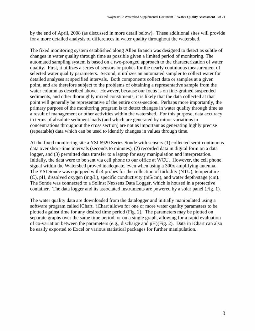
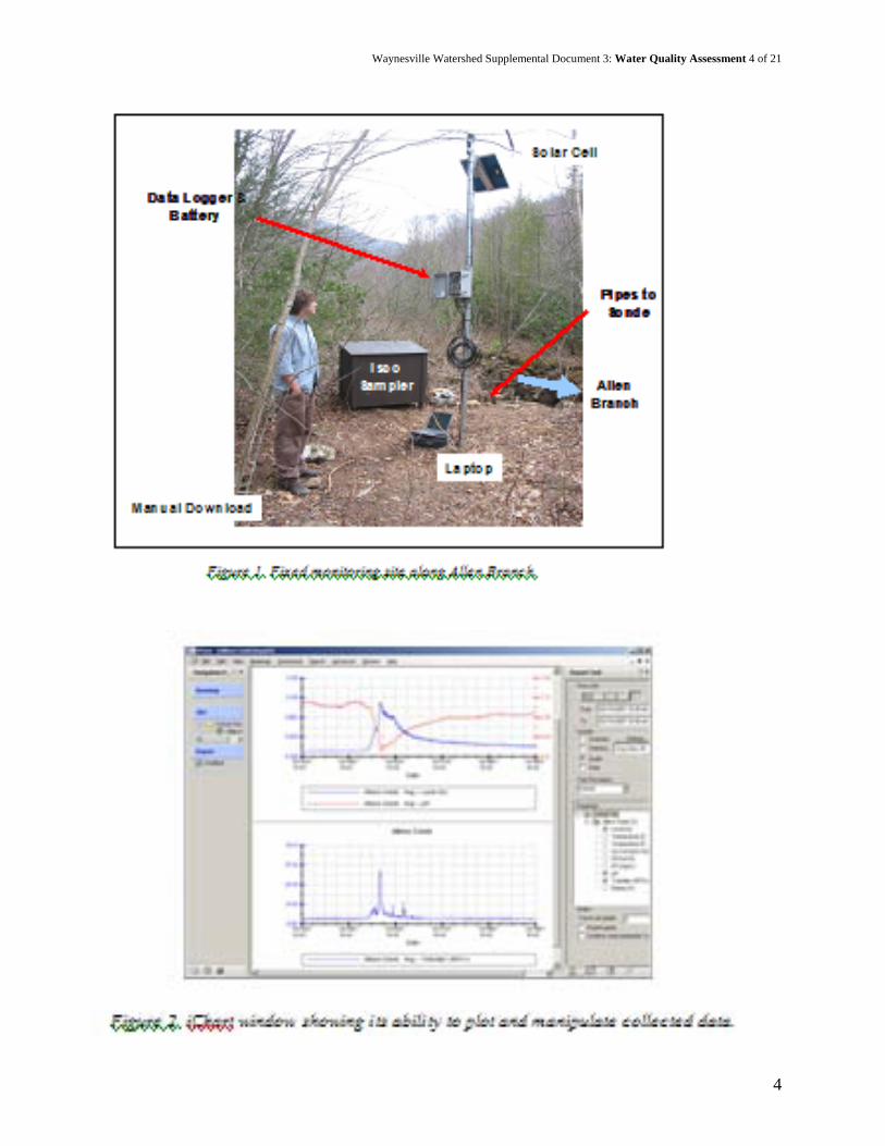
by the end of April, 2008 (as discussed in more detail below). These additional sites will provide for a more detailed analysis of differences in water quality throughout the watershed. The fixed monitoring system established along Allen Branch was designed to detect as subtle of changes in water quality through time as possible given a limited period of monitoring. The automated sampling system is based on a two-pronged approach to the characterization of water quality. First, it utilizes a series of sensors or probes for the nearly continuous measurement of selected water quality parameters. Second, it utilizes an automated sampler to collect water for detailed analyses at specified intervals. Both components collect data or samples at a given point, and are therefore subject to the problems of obtaining a representative sample from the water column as described above. However, because our focus is on fine-grained suspended sediments, and other thoroughly mixed constituents, it is likely that the data collected at that point will generally be representative of the entire cross-section. Perhaps more importantly, the primary purpose of the monitoring program is to detect changes in water quality through time as a result of management or other activities within the watershed. For this purpose, data accuracy in terms of absolute sediment loads (and which are generated by minor variations in concentrations throughout the cross section) are not as important as generating highly precise (repeatable) data which can be used to identify changes in values through time. At the fixed monitoring site a YSI 6920 Series Sonde with sensors (1) collected semi-continuous data over short-time intervals (seconds to minutes), (2) recorded data in digital form on a data logger, and (3) permitted data transfer to a laptop for easy manipulation and interpretation. Initially, the data were to be sent via cell phone to our office at WCU. However, the cell phone signal within the Watershed proved inadequate, even when using a 300x amplifying antenna. The YSI Sonde was equipped with 4 probes for the collection of turbidity (NTU), temperature (C), pH, dissolved oxygen (mg/L), specific conductivity (mS/cm), and water depth/stage (cm). The Sonde was connected to a Solinst Nexsens Data Logger, which is housed in a protective container. The data logger and its associated instruments are powered by a solar panel (Fig. 1). The water quality data are downloaded from the datalogger and initially manipulated using a software program called iChart. iChart allows for one or more water quality parameters to be plotted against time for any desired time period (Fig. 2). The parameters may be plotted on separate graphs over the same time period, or on a single graph, allowing for a rapid evaluation of co-variation between the parameters (e.g., discharge and pH)(Fig. 2). Data in iChart can also be easily exported to Excel or various statistical packages for further manipulation.


4


5

Selection of the monitoring site was based on accessibility (particularly during storm events), pool depth (required for monitoring during dry summer months), and upstream basin area (assuming the more area encompassed by the monitoring system, the better). Stability of the channel was also an important criteria to insure that significant changes in stage-discharge relations did not occur during major flood events. The Sonde was initially installed along Allen Branch on November 6, 2006, approximately 0.5 mi upstream of the confluence between Cherry Cove Creek and Deep Gap Creek (Fig. 3). Allen Branch is one of four main tributaries to the reservoir and drains the largest area within the watershed. The station includes a monitoring area of approximately 1990 ac, or approximately 27 % of the Watershed. During this initial sampling period, which continued through February 10, 2007, the Sonde was anchored directly in the channel, and was not equipped with either the turbidity probe or pressure transducer. It was subsequently moved a short-distance downstream on March 03, 2006 where it was fixed in place and the turbidity probe and pressure transducer were added to the array of instruments. It has continuously collected data at the site since its installation in March, 2007. Our discussion here will be on data collected through February 4, 2008. The collection of suspended sediments utilized an Isco 6712 Automated Water sampler. The use of an automated sampler was considered necessary to adequately document changes in suspended sediment and other contaminant concentrations during storm runoff. Higher suspended sediment concentrations during floods have led to the concept of stratified sampling. A stratified sampling approach typically involves the collection of numerous samples during floods, a time when significant variations in suspended sediment concentration are occurring, and limited sampling during low flow conditions when variations in parameter values are generally negligible. Stratified sampling almost always requires an automated sampling system, which allows the onset of sampling to be triggered by changes in some measurable parameter, such rainfall, a change in stage, velocity, or discharge, or alterations in pH, electrical conductivity, turbidity or specific ions. In our case, sampling was trigged by a change in stream water level. Once sampling began, the intervals between collection of samples were set for a uniform increment of time (time-sequenced sampling), or followed an algorithm that allowed the sampling intensity to be adjusted to real-time flow conditions (event-stratified sampling). In addition to continuous water quality data, precipitation data (amount, duration, and intensity) were needed to fully understand the drivers of water quality variations during storm events. Precipitation data were acquired from a TVA weather station located approximately two miles from the water quality-monitoring site. The weather station is located at the Waynesville Municipal Water plant. Precipitation data are recorded every 15 minutes with a tipping bucket rain gage accurate to the nearest hundredth of an inch. It should be noted that the precipitation records at this site may not be representative of the entire watershed because of variability within the watershed. Potential error would be greatest during short, small intense storms (e.g. thunderstorms).


6


7

3 Water Quality Results 3.1 General Statistics Data were collected at two sites during the monitoring period. At site 1, pH, electrical conductivity, dissolved oxygen, and temperature were collected from November 6, 2006 through February 10, 2007. Data were then collected for the same parameters plus stage, turbidity, and TSS from the fixed site from March 3, 2007 to the present (Fig. 3). The results from both sites are similar, but because data from the fixed site includes measurements of stream flow (stage) and turbidity, our discussion will focus on the fixed site unless otherwise noted. During the period of monitoring, there were more than 60,000 measurements made of turbidity, pH, electrical conductivity, stage, and dissolved oxygen at the fixed monitoring site (Site 2). The collected data reveal that water quality within Allen Branch is in very good condition, at least for the parameters measured. None of the parameters regularly fell within a range that would be detrimental to aquatic biota (Table 1). For example, trout are thought to show signs of stress when subjected to waters with a turbidity value in excess of approximately 10 NTU for a period of hours. Maximum turbidity exceeded 10 NTU a total of 14 times, but only for short periods, on average about 1.20 hours (Fig. 4a). In fact, turbidity values were less than 2.5 NTU, and close to the level of detection, for 99 % of the time (Fig. 4b). As an illustration of how clear the water actually is, water with a turbidity of <5 NTU can be used for consumption provided that it is not contaminated by microbes. It is also important to recognize that other streams in the region which lie within developed areas exhibit turbidity values on the order of several thousand NTUs during flood events. Table 1. Descriptive statistics for selected water quality parameters measured at the fixed monitoring site between March 3, 2007 and February 4, 2008.

Statistic

Stage (m)

Temp (C)

Specific Conductivity (μS/cm)

pH Turbidity (NTU)

Mean 0.44 10.73 17.73 7.13 1.05 Standard Dev. 0.06 5.06 3.12 0.13 1.76 Minimum 0.34 0.04 <1.00 4.31 <1.00 Maximum 0.97 21.61 39.00 7.43 93.20 (# of measurements)

60764 60752 60764 60764 60732

NC Guidelines* --- <29 --- <~6; >~9

<10

* - North Carolina State Water Quality Guidelines for Class C Waters (trout water designation)


8

Figure 4. (A) Average time during which turbidity exceeded specified values during floods; (B) frequency of turbidity measurements during the monitoring

period.

0 .00

0 .20

0 .40

0 .60

0 .80

1.00

1.20

1.40

>10 >20 >30 >40 >50 >60 >70 >80 >90

T urbidit y C ate go ries

Turbid it y (NTU) Values

14 S t o r ms

11 S t or ms

9 S t or ms

7 S t or ms5 S t or m s

4 S t or ms 3 S t or ms 2 S t or m s

1 S t or ms

0.000

10.000

20.000

30.000

40.000

50.000

60.000

70.000

80.000

90.000

100.000

0-2.5 2.5-5 5-10 10-20 20-30 30-50 50-100 100-200Turbidity (NTU) Value Catergories

Pere

cent

of T

ime

B

A


9

Turbidity is a measure of the degree to which substances in the water (both dissolved and suspended with the water column) attenuate or scatter a beam of light. It is often used in regulations because it is easier to measure than the total suspended solids content of the water. However, turbidity values are affected by more than just the concentration of suspended particles. Dissolved constituents can dramatically influence turbidity, as can the size and shape of the particles that are present. As a result, many scientists prefer to rely on TSS measurements when quantifying water quality. TSS refers to the total mass of solid material in the water (included mineral matter, algae, and plant debris) that can be separated by means of filtration. Unlike turbidity, regulations related to TSS values are typically based on comparisons with background or reference values measured for the region. Unfortunately, quantitative data for this area are lacking. Nevertheless, toxic effects to trout are likely to be on the order of a hundred to a few hundred mg/L. Of the 292 samples which were collected and analyzed, nearly 70 % exhibited TSS values of less than 2 mg/L (Fig. 5). The highest values occurred during flood events, but none of the collected samples exceeded 90 mg/L. The TSS data, like the turbidity data, indicate that suspended sediment loads are very low within Allen Branch. The exceedingly clean water may come as a surprise given the basin’s previous history and the extent of roads which remain. The low TSS and turbidity values are likely to result from a combination of factors, including (1) gullies and ditches along the margins of the roads have largely healed, are vegetated, and do not transmit large amounts of water and sediment, (2) roads and other sources of upland sediment are not well integrated with the drainage network, inhibiting in the influx of large amounts of sediment to the channel, (3) although the channel is locally incised and locally characterized by vertical banks, the exposed bank materials are largely composed of bedrock and coarse debris which forms relative stable banks and is hard to transport once bank failure occurs, and (4) the vast majority of the watershed maintains healthy soils with high infiltration capacities, so that very little storm runoff (especially overland flow) is generated.

0

10

20

30

40

50

60

70

80

90

100

0-2 2-5 5-10 10-15 15-30 30-50 50-70 70-90 >90

Total Suspended Solids (ppm) Category Range

Perc

ent o

f Mea

sure

men

ts

TSS (ppm)Total number of measurements is 292, includes data from16 storms, as well as some periods of intervening baseflow.

Figure 5. Percent of samples for specific TSS ranges.


10

3.2 Temporal Variations Figures 6 and 7 show that measured water quality parameters vary through time as a function of the water level within the stream (stage). Variations in both turbidity and TSS were pronounced during floods, with the values of each increasing during the rising stages of the flood, and decreasing thereafter (Figs. 6, 7). Given the dependency of the sediment load on discharge, it is essential to consider the influence of stream flow on turbidity and TSS when attempting to determine changes in water quality. One of the easiest ways of doing this is to develop a bivariate relationship between discharge and turbidity or discharge and TSS. In most cases, these statistical relationships are best defined when the values are plotted in log-log space. Once developed, water quality data for a given set of flow conditions following a disturbance can be compared to the statistical relationships to determine if the values fall within the typical range of values observed prior to the event. This process is not as easy as you might think because there is generally significant variation in the data that form the trend between discharge and turbidity or TSS. In the case of Allen Branch, a relationship between stage (a surrogate for discharge) and turbidity could not be developed. As Figure 8 shows, stage-turbidity relations follow several different trends, even when the values are adjusted for base flow water level at the onset of the runoff event. It is not entirely clear at this time why so much variability exists in the data, but several factors are likely to be of importance. First, the range over which turbidity varies is limited. Thus, the influx of even minor amounts of sediment or organic debris can have a major influence on turbidity. Second, suspended sediments are usually supply limited. This means that the stream during floods always has the ability to transport the suspended sediment delivered to the channel. The actually suspended sediment load depends on the amount of sediment which enters the channel during runoff from upland areas. Sediment delivery is controlled by a large number of parameters such as the amount of runoff (versus subsurface water), the antecedent moisture conditions, the connectivity of the upland sediment sources with the channel, and the intensity, duration, and frequency of the precipitation events. Multivariate regression analysis suggested that part of the variation in turbidity was related to antecedent moisture conditions (where antecedent moisture is quantified by the amount of time between storm events). When storms were spaced at least four days apart (and not significant impacted by high antecedent moisture), as much as 82 % of the variation in peak flood turbidity could be explained by storm intensity alone (Fig. 10). The relations between TSS and stage are also weak; in fact, no statistically significant relationship could be developed (Fig. 9). When combined with the turbidity data, the TSS measurements suggest that suspended sediment loads are likely to vary as a function of different storm/runoff regimes, where runoff regimes are a function of storm duration, intensity, and antecedent moisture conditions. In order to separate the data into specific populations, we will need to apply more sophisticated multivariate statistical techniques to a larger dataset than is currently available.


11

2/1/

2007

3/1/

2007

4/1/

2007

5/1/

2007

6/1/

2007

7/1/

2007

8/1/

2007

9/1/

2007

10/1

/200

7

11/1

/200

7

12/1

/200

7

1/1/

2008

2/1/

2008

3/1/

2008

0.20.40.60.81.0

DATE

Stag

e (m

)

6.5

7.0

7.5

pH

1

10

100

Turb

(NTU

)

1012141618202224

Con

d.(u

S/cm

)

05

10152025

Tem

p. (C

)

2/1/

2007

3/1/

2007

4/1/

2007

5/1/

2007

6/1/

2007

7/1/

2007

8/1/

2007

9/1/

2007

10/1

/200

7

11/1

/200

7

12/1

/200

7

1/1/

2008

2/1/

2008

3/1/

2008

0.20.40.60.81.0

DATE

Stag

e (m

)

6.5

7.0

7.5

pH

1

10

100

Turb

(NTU

)

1012141618202224

Con

d.(u

S/cm

)

05

10152025

Tem

p. (C

)

Figure 6. Variations in selected water quality parameters from March 3, 2007 through the end of February, 2008. Note how the parameters change with

changes in stage (discharge).


12

9/13/2007 9/15/2007 9/17/20070.20.40.60.81.0

Date

Sta

ge (m

)

6.0

6.5

7.0

7.5

pH

020406080

Turb

. (N

TU)

15

20

25

Con

d.(u

S/c

m)

101214161820

Tem

p. (C

)

9/13/2007 9/15/2007 9/17/20070.20.40.60.81.0

Date

Sta

ge (m

)

6.0

6.5

7.0

7.5

pH

020406080

Turb

. (N

TU)

15

20

25

Con

d.(u

S/c

m)

101214161820

Tem

p. (C

)

Figure 7. Variations in selected water quality parameters from March 16-18, 2007 (an individual flood). Note how the parameters change with changes in

stage (discharge).


13

0.01 0.02 0.04 0.06 0.080.1 0.2 0.4 0.61

2

4

68

10

20

40

6080

100

200

Turb

idity

(NTU

)

Stage above baseflow (m)

Figure 8. Variations in turbidity as a function of water level above baseflow. The lack of a statistical trend suggests that factors in

addition to discharge on controlling turbidity.

0.0

0.1

1.0

10.0

100.0

0.1 1

Stage Level (m)

Tota

l Sus

pend

ed S

olid

s (p

pm)

Figure 9. Changes in TSS as a function of discharge. Data collected between March 3, 2007and February 5, 2008.


14

In addition to variations in turbidity and TSS during floods, the data reveal that variations in flood characteristics and sediment loads occur on a seasonal basis. Storms which occurred during the summer tended to generate lower peak discharges (Fig. 6), but were more intense and generated higher values of turbidity. Thus, analysis of the potential changes in water quality following a management activity will need consider the season during which the activity was performed and the monitoring data collected. In an ideal situation, strong statistical relationships exist between turbidity and TSS. Where this occurs, the nearly continuously collected turbidity measurements can be used to estimate the total suspended solids load. In the case of Allen Branch, the relationship between turbidity and TSS is statistically significant (p<0.05), but the relationship is rather weak (Fig. 11). 4 Hysteresis and Possible Sediment Sources Hysteresis is a phenomenon that occurs when the timing of maximum elemental concentrations do not precisely correlate with the timing of the peak flood flow. It is an important consideration in monitoring programs because different values of TSS (or turbidity) occur for a given discharge, depending on whether it is associated with the rising or falling limb of the hydrograph. It therefore produces much of the scatter in the discharge-TSS/turbidity relationships described above. Williams (1989) identified 4 possible types of hysteresis, in addition to linear relationships between sediment concentration and discharge (Fig. 12). Exactly which type of hysteresis is formed, if any, depends on the interaction of a large number of factors, including sediment availability, the intensity and areal distribution of precipitation within the basin, the amount and rate of runoff, the amount of sediment stored along the channel, and differences in downstream flow rates between the sediment and water (Williams, 1989). The most

R2 = 0.8264P = 0.00017

n = 13

0

50

100

150

200

250

0.00 0.10 0.20 0.30 0.40 0.50 0.60 0.70 0.80 0.90 1.00

Maximum Storm Intensity (inches/hour)

Max

imum

Sto

rm T

urbi

dity

(NTU

)

Note: Storms within 4 days of anotherstorm were omitted due to the influence of antecedent moisture conditions.

Figure 10. Relationship between TSS and maximum storm intensive between March 3, 2007 and February 5, 2008 at the fixed station.


15

commonly observed type of hysteresis (represented by a clockwise loop) occurs where suspended sediment concentrations reach a maximum before peak flow is attained (Fig. 12). It is generally attributed to the input of easily eroded sediment to the channel during the early stages of a runoff event, followed by a decline in sediment influx as the easily eroded materials are depleted from upland areas (Williams, 1989; Knighton, 1998). Turbidity measured at the fixed station of Allen Branch consistently exhibited a clockwise hysteretic relationship during the 34 floods examined during the monitoring period (Fig. 13a). It appears, then, that increases in turbidity were associated with the input of sediment (particularly easily transported organic debris, silt, and clay) to the channel during the early stages of the flood. This observation is consistent with the observation that peak turbidity correlated with peak storm intensity, and the movement of sediment off of upland areas during the most intense periods of a precipitation event (which generally precede peak flood levels within the channel). In contrast to turbidity, TSS was observed to frequently exhibit a counter-clockwise hysteretic loop (Fig. 13b). This type of hysteresis may be related to differences in the rate at which water and suspended sediments move through the channel (Knighton, 1998). In headwater areas, hillslope processes can deliver sediment to the channel relatively quickly, allowing suspended sediment concentrations to peak during the early stages of an event, producing clockwise loops. However, peak flow conditions may

0.1 1 10 1000.1

1

10

100

Turb

idity

(NTU

)

Total Suspended Solids (mg/L)

R2=0.3078

Figure 11. Changes in turbidity as a function of total suspended sediment concentration. Ideally, turbidity could be used to predict TSS values.


16

occur downstream, in our case at the fixed station, before maximum suspended sediment concentrations are realized because flood waves move considerably faster than the suspended particles. The shift in the timing of peak discharge relative to maximum suspended sediment concentration produces a reversal in the rotational direction of the hysteretic loop. An alternative possibility, which we favor, is that sediment comprising samples collected for TSS analysis is different from that causing turbidity. While there was not enough sediment captured in the TSS samples for quantitative analysis, inspection of the samples showed that the particulate matter was primarily composed of organic material and fine- to medium-sand sized particles. Because of the density differences of the two types of materials, the mineral matter is likely to dominate the TSS measurements. It is possible, if not likely, that the sand-sized particles were derived from the erosion of the channel banks during peak flow conditions, thereby creating the observed counter-clockwise hysteretic loop in TSS, while the turbidity was primary associated with organic debris flushed in from upland areas. This hypothesis would also account for the high degree of variability between turbidity and TSS. These observations

Figure 12. Types of hysteresis recognized by Williams (1989). Figure from Miller and Orbock Miller (2007).


17

are important because changes in the nature of the hysteretic loops, particularly for TSS, following a management activity may indicate a new and predominant source of sediment to the channel. 5 Discussion and Summary of Results Stream waters within the downstream reaches of Allen Branch were found to be of exceptionally quality for the parameters evaluated. Given the watersheds past history, the findings are a

Storm 8, Allen Branch, Turbidity (NTU) plotted against Stage (m)

0

5

10

15

20

25

30

35

40

45

0 0.2 0.4 0.6 0.8 1 1.2

Stage (m)

Time 00:00

05:45

08:15

12:15

49:45

Storm 8, Total Supsended Solids (ppm) plotted against Stage (m), Allen Branch, Waynesville, NC, 3/16/07

0

10

20

30

40

50

60

70

80

0 0.2 0.4 0.6 0.8 1Stage (m)

Time 00:00

09:30

11:30

15:30

19:30

49:45

B

AStorm 8, Allen Branch, Turbidity (NTU) plotted against

Stage (m)

0

5

10

15

20

25

30

35

40

45

0 0.2 0.4 0.6 0.8 1 1.2

Stage (m)

Time 00:00

05:45

08:15

12:15

49:45

Storm 8, Total Supsended Solids (ppm) plotted against Stage (m), Allen Branch, Waynesville, NC, 3/16/07

0

10

20

30

40

50

60

70

80

0 0.2 0.4 0.6 0.8 1Stage (m)

Time 00:00

09:30

11:30

15:30

19:30

49:45

B

A

Figure 13. (A) Clockwise hysteresis exhibited by turbidity; (B) counter-clockwise hysteresis often exhibited by TSS. Both graphs developed from data collected

during the March 16, 2006 runoff event.


18

somewhat surprising, and attests to the region’s ability to rapidly recover from intense disturbances. The highest measurements of turbidity and TSS were associated with floods, but typically developed relationships between discharge (stage) and sediment load (TSS, turbidity) were weak (Figs. 11, 12). The high degree of variability is most likely due to (1) the limited range of values that were measured, (2) differences in the influx of sediment during storm events as a result of varying precipitation intensities, duration, antecedent moisture conditions, and season, (3) hysteresis affects, and (4) differences in the type and source of sediment that comprise the total suspended solids and which causes increases in turbidity. The absence of strong statistical relationships between stage and turbidity or stage and TSS reduces our ability to determine changes in water quality as a result of watershed disturbance. However, other approaches can be used to identify changes in water quality, such as an analysis of the frequency of which turbidity of a given value (e.g., 10 NTU) occur during or following a management activity (discussed in more detail below). It is also important to recognize that the high quality of the water, and the sensitivity of our instrumentation, should allow the system to detect even minor inputs of sediment to the channel. Thus, the question that may arise is not whether we will be able to detect a change in water quality, but rather, what level of change is considered acceptable. We argue that criteria (or guidelines) regarding what is acceptable should be developed before any management activity is undertaken to avoid confusion as to what is considered a successful management operation. 6 Assessment of Management Activities To date our attention has focused on the collection of high quality data from a single point within the channel, a process that has provided detailed insights into the geochemical nature of the water entering the reservoir and the variations in selected water quality parameters through time. Our future monitoring activities will expand upon these fixed point data by collecting semi-continuous data at an additional 5 sites within the watershed to enhance our understanding of the spatial variations in water quality within the basin. These additional sites, which we expect to have installed by the end of April, 2008, will be instrumented with two devices, including a Solinst pressure transducer and a Stevens turbidity probe. The pressure transducers provide information on surface water elevations, flow depths, and temperature within the channel, thereby allowing for the estimation of discharge. These particular devices are self-contained, meaning that they both record and store the information in a digital format until it is downloaded onto a laptop for easy manipulation. They can be placed within a stilling well on the side of the channel or, more frequently, within a perforated metal pipe anchored in the channel. We typically collect depth measurements at 5-minute time intervals. The Stevens turbidity probes are also designed for the collection and storage of continuous data in a digital format. Three of the units are self-contained and can be installed directly in the channel, while the remaining two units are linked via a cable to 12-Volt (marine) battery along the side of the channel. Both types allow for the collection of turbidity measurements at sub-minute intervals, although we will likely collect information at 5-minute increments. Because the utilized probes can be easily moved, these roaming site monitoring stations will allow for a detailed analysis of the spatial variations in discharge within the watershed prior to any management activities.


19

The potential impacts of future management activities on water quality will be determined using a multi-pronged approach which involves the collection of data over differing scales of space and time. Because the investigated water quality parameters vary as a function of the flow conditions within the channel, the magnitude of the measured parameters must be interpreted on the basis of the discharge for which they were collected. Thus, a common approach to determine changes in water quality in other areas has been to document differences in the statistical relationships between discharge and total suspended solids (TSS), or between discharge and turbidity. Although such an approach is now possible using data from the fixed monitoring station, the relationships between these variables in the Waynesville watershed are extremely weak. The approach, then, will need to be modified to identify changes in water quality (unless changes in TSS or turbidity are on the scale of an order of magnitude or more). Improvements upon the approach will likely involve the development of discharge – turbidity/TSS relationships for specific types of flood events, where flood types are classed according to storm intensity, season, etc. as discussed earlier. The approach should allow for the development of much stronger discharge-TSS/turbidity relationships, and for the identification of more subtle changes in water quality. A closely related methodology using the fixed station data will be to examine peak TSS and turbidity values for individual storms of a given storm type, and the nature of the hysteretic loops which accompany them. This will provide insights into changes in the peak values which occur, if any, as well as potential changes in the source of those sediments (as described earlier). In addition to the examination of discharge-turbidity/TSS relations, we will monitor changes in the frequency with which flows of a given turbidity or TSS occur. This approach will involve the development of frequency histograms and cumulative frequency curves depicting the frequency during which flows of a given turbidity or TSS occur during a 6-month period. For example, these data may show that for a given six month period, a turbidity value of 10 NTUs was exceeded 1 percent of the time. Clearly, this approach represents a long-term analysis of water quality change, but one which is likely to identify even minor alterations in TSS or turbidity and be indicative of cumulative impacts. Data from the roaming sites, instrumented with stage (water depth), temperature, and turbidity probes, will also be extensively utilized to identify potential changes in water quality. These analyses fall into two categorizes: at-a-station analyses and a paired-basin type analyses. At-a-station analyses will involve the collection of stage (water level), temperature, and turbidity data from one or more sites located immediately downstream of planned management activities, and the comparison of data collected prior to the disturbance to that collected during and following the disturbance. It will be important to locate the roaming stations downstream of the site months in advance (the longer, the better) to obtain as much information on the variability in runoff and sediment loads as possible. In terms of indices, we will concentrate on changes in peak turbidity values during storm events of a given magnitude/frequency range as well changes in the overall frequency with which flows of a given turbidity occur. These indices have proven effective in characterizing water quality responses to storms in the data collected to date. Turbidity is primarily a function of suspended matter. Thus, it will also be necessary to monitor changes in the particle size distribution of the channel bed material to determine if sand-sized or


20

finer sediments are accumulating on (in) the channel bed. Changes in bed material composition will be monitored by selecting 3-6 monitoring sites downstream of the management activity and visually documenting the site’s bed material composition, both in the field and through the comparison of photographs of the channel bed, consistently obtained from the same location. Changes in bed composition indicate changes in the sediment budget of a stream and may indicated changes in stream habitat quality. The paired-basin approach involves the comparison of discharge-turbidity relations of subbasins where management activities are ongoing with subbasins where they are not. This approach relies on data from the roaming stations, which be will installed in 2008. An assumption inherent in the approach is that the control and disturbed subbasins are similar in character. To account for the possible effects of differing basin size, geology, soils, relief, etc. on sediment loads, it may be necessary to normalize the collected information. There are a number of new, more sophisticated methods of determining the source and timing of sediment to the channel, which may be utilized if funding of these experimental approaches can be obtained. One possible approach involves an examination of the short-lived radionuclide content of the channel bed sediment before, during, and after the management activities. Cesium-137, for example, is a product of nuclear bomb tests of the 1950s and early 1960s. Fallout over North America reached a maximum in 1963, after which its concentrations have declined. In many area, Cs-137 is concentrated in surface soils and its concentration within in a stream channel is related to (1) the amount of upland soil erosion, (2) its mixing with sediment derived from other sources low in Cs-137, such as bank materials, or from deeply eroded gullies, and (3) the residence time of sediment within the channel. Thus, it may be possible to document changes in the source and contribution of sediments to the channel bed by examining alterations in the Cs-137 content of the channel bed sediments before and after management activities have occurred. Similar analyses may also be undertaken using Be-57. A disadvantage of these methods is that they are relatively expensive; thus, they will only be performed if funding can be obtained. Another experimental study that could be performed if additional funding is secured is to assess the impact of management activities on basin hydrology. For example, commonly there is an increase in overland flow and soil erosion in disturbed land. With the increase in overland flow, there is a reduction in the recharge of groundwater. To better understand any hydrologic impacts of management, as well as potential reasons for changes in sedimentation, studies to determine the pathways of water and the water budget would need to be carried out. There are numerous ways to carry out such a study, but most would involve utilizing chemical and physical traits of water to make inferences about hydrologic pathways. For example, during the summer months, groundwater typically has cooler temperatures, a higher pH, and a high conductivity than storm runoff waters. These traits are reflected in the water quality collected in the Waynesville watershed at the fixed station; stream pH tends to drop during storms because groundwater makes up less of the stream flow (Fig. 6). A related method is to monitor stream bed temperatures paired with the temperature about 15 cm below the bed of the stream (temperature data loggers would be used to collect the data and operate similar to other loggers described previously). By analysis of the temperature trends at these paired locations, inferences can be made about the locations and amounts of groundwater contributing to a stream.


21

7 References Feltz HR, Culbertson JK (1972) Sampling procedures and problems in determining pesticide

residues in the hydrologic environment. Pesticide Monitoring Journal 6:171-178 Horowitz AJ (1990) Variations in suspended sediment and associated trace element

concentrations in selected riverine cross sections. Environmental Science and Technology 24:1313-1320

Knighton D (1998) Fluvial forms and processes: a new prospective, Arnold, London Miller J, Orbock Miller SM (2007) Contaminated Rivers: A Geomorphological-Geochemical

Approach to Site Assessment and Remediation. Springer, Berlin. Thomas RB, Lewis J (1995) An evaluation of flow-stratified sampling for estimating suspended

sediment loads. Journal of Hydrology 170:27-45 Williams GP (1989) Sedment concentration versus water discharge during single hydrologic

events in rivers. Journal of Hydrology 111:89-106

water quality assessment 1. background - e-gov link · comparing integrated and pump sampling...

Documents