Alexandria Engineering Journal (2013) 52, 67–81

Alexandria University

Alexandria Engineering Journal

www.elsevier.com/locate/aejwww.sciencedirect.com

ORIGINAL ARTICLE

Optimizing strategy for repetitive construction

projects within multi-mode resources

Remon Fayek Aziz *

Structural Engineering Department, Faculty of Engineering, Alexandria University, Egypt

Received 10 September 2012; revised 13 November 2012; accepted 20 November 2012Available online 21 December 2012

A

C

Ba

PB

O*

E-

Pe

U

11

ht

KEYWORDS

Tendering;

Construction repetitive

projects;

Line Of Balance;

Cash flow;

Net present value;

Mathematical modeling and

multi-objective optimization

bbreviations: AI, Artificial Int

ritical Path Method; DCF, D

lance; NPV, Net Present Val

P, Pay Back Period; PDM, P

ptions; TASC, The Advanced

Tel.: +20 12 2381 3937.mail address: Remon_fayek@

er review under responsibility

niversity.

Production an

10-0168 ª 2013 Faculty of E

tp://dx.doi.org/10.1016/j.aej.2

elligence;

iscounte

ue; P6, P

recedenc

S-Curve

hotmail

of Facu

d hostin

ngineerin

012.11.0

Abstract Estimating tender data for specific project is themost essential part in construction areas as

of a contractor’s view such as: proposed project duration with corresponding gross value and cash

flows. Cash flow analysis of construction projects has a long history and has been an important topic

in construction management. Determination of project cash flows is very sensitive, especially for

repetitive construction projects. This paper focuses on how to calculate tender data for repetitive con-

struction projects such as: project duration, project cost, project/bid price, project cash flows, project

maximumworking capital and project net present value that is equivalent to net profit at the beginning

of the project. A simplified multi-objective optimization formulation will be presented that creates

best tender data to contractor comparing with more feasible options that are generated from multi-

mode resources in a given project. This mathematical formulation is intended to give more scenarios

which provide a practical support for typical construction contractors who need to optimize resource

utilization in order to minimize project duration, project/bid price and project maximum working

capital while maximizing its net present value simultaneously. At the end of the paper, an illustrative

example will be presented to demonstrate the applications of proposed technique to an optimization

expressway of repetitive construction project.ª 2013 Faculty of Engineering, Alexandria University. Production and hosting by Elsevier B.V.

All rights reserved.

CB, Capital Budgeting; CPM,

d Cash Flow; LOB, Line Of

rimavera enterprise Version 6;

e Diagram Method; RO, Real

.

.com

lty of Engineering, Alexandria

g by Elsevier

g, Alexandria University. Product

03

1. Introduction

Unlike the traditional price-focused lowest bid, the best value

tendering process selects the contractor who offers a product/work that is most beneficial to the procurement entity withvarious aspects [1]. In recent years, as both sides of construc-

tion industry (contractors and clients) have become aware ofthe good cash flow management advantages, there have beenmany attempts to devise an accurate method of predicting

the cash flow pattern of a construction project in advance. Tra-ditional approaches to cash flow prediction usually involvedthe breakdown of the bill of quantities in line with the contract

program to produce an estimated expenditure profile. This

ion and hosting by Elsevier B.V. All rights reserved.

Net Cash Flow

Negative Cash Flow (Disbursements)

Positive Cash Flow (Receipts)

Variously Known as

Variously Known as

• Liability • Expenditure • Cost • Cash Out

• Earnings • Income • Value • Cash In

Expended On Derived From

• Materials • Labors • Plant • Subcontractor • Preliminaries • Overheads

• Materials • Labors • Plant • Subcontractor • Preliminaries • Overheads

Figure 1 Construction cash flow concept (Source: [15]).

68 Remon Fayek Aziz

could be expected to be reasonably precise provided that bill ofquantities is accurate and the contract program is compliedwith. However it is likely to be costly to produce unless the bill

is in operational format. Financial management has long beenrecognized as an important management tool and proper cashflow management is crucial to the survival of a construction

company because cash is the most important corporate re-source for its day-to-day activities [2,3]. A proper cash flowmanagement is also important as a mean of obtaining loans,

as banks and other money lending institutions are normallymuch more inclined to lend money to companies that can pres-ent periodic cash flow forecasts [4]. However, constructionindustry suffers the largest numbers of bankruptcy in any sec-

tor of the economy with companies failing as a result of poorfinancial management, especially inadequate attention to cashflow management [5–7]. One of the final causes of bankruptcy

is inadequate cash resources and failure to convince creditorsand possible lenders of money that this inadequacy is onlytemporary. The need to forecast cash requirements is impor-

tant in order to set provision for these difficult times beforeHarris and McCaffer arrive [7]. Cash flow forecasting accord-ing to McCaffer [8] provides a good warning system to predict

possible insolvency. This, according to McCaffer [8], enablespreventive measures to be considered and takes in good times.Many approaches to cash flow forecasting have been reportedin literature [9–11]; also many approaches to cash flow man-

agement abound in literature [7,12,13]. However, the construc-tion industry’s awareness and usage of these approaches is yetto be investigated. This, then, is the concern of this study.

2. Cash flow management approaches

Cooke and Jepson [14] defined cash flow as the actual move-

ment of money in and out of a business. Money flowing intobusiness is termed ‘‘positive cash flow’’ and is credited as cashreceived. Monies paid out are termed ‘‘negative cash flow’’ and

are debited to the business. The difference between the positiveand negative cash flows is termed the ‘‘net cash flow’’. As thereare different views held about what cash flow means in litera-

ture, cash flow as defined by Cooke and Jepson [14] is the viewupheld in this study and has been conceptualized by Odeyinkaand Lowe [15] and shown in Fig. 1.

According to Cooke and Jepson [14], within a construction

organization, positive cash flow is mainly derived from moniesreceived in the form of monthly payment certificates. Negativecash flow is related to monies expended on a contract in order

to pay wages, materials, plant, sub contractors’ accounts ren-dered and overheads expended during the work progress.According to them, on a construction project, the net cash flow

will require funding by contractor when there is a cash deficit,and where cash is in surplus, the contract is self-financing.Short-term bank loans or overdraft facilities according toCormican [13] often meet the shortfall that may occur between

the supply of funds and the need for cash. In recent years how-ever, according to Cormican [13], the credit facilities extendedby financial institutions have been subject to more strict con-

trols, and this has often resulted in cash shortages in firms thatmay not suspect a threat from this source. The resulting short-age of cash may often force liquidation of assets and foreclo-

sure by the company’s creditors. A contractor may be forcedto avail himself of short-term borrowing at very high interest

rates [13]. Other approaches utilized in resolving cash deficitaccording to Harris and McCaffer [7], Kaka and Price [16] in-clude delayed payment to subcontractors and suppliers; tender

unbalancing, utilizing company’s cash reserves and overvalua-tion. Mawdesley et al. [17] emphasized the need for financialplan in cash flow management. This, according to Mawdesley

et al., would normally represent the planned position through-out a project and as such would be concerned with the income,expenditure and net cash flow. This enables the cash flow situ-ation to be monitored using approaches such as pre-project

cash flow plan or forecast, project phase monitoring/updatingand monthly cost/value reconciliation. Kaka and Boussabaine[9] and Mawdesley et al. [17] emphasized the need to update

cash flow forecast in the course of a project. The suggested fre-quency of updating cash flow forecast from these, andother authors include weekly, monthly and quarterly update.

Cormican [13] is however, of the opinion that updates shouldbe done when the deviations from the existing plan are mean-ingless, or when the client requests an update. The traditional

approach to cash flow prediction usually involves the break-down of the bill of quantities in line with the contract programto produce an estimated expenditure profile. This could be ex-pected to be reasonably precise, provided that the bill of quan-

tities is accurate and the contract program is complied with[18]. Although this traditional approach is presently being sup-plemented with the use of computer spreadsheet, it is likely to

be slow and costly to produce; as such, several attempts havebeen made to devise a ‘short cut’ method of estimation, whichwill be both quicker and cheaper to utilize. Attempts have been

made at the mathematical formulae and statistical based mod-eling of construction cash flow in both contractor’s and client’sorganizations. This was demonstrated by many researchersthrough developing a series of typical S-curves [16]. The mod-

els obtained by these researchers rest on the assumption that

Optimizing strategy for repetitive construction projects within multi-mode resources 69

reasonably accurate prediction is possible by means of a singleformula utilizing two or more parameters which may varyaccording to the type, nature, location, value and duration

of the contract. Kenley [10] identified other cash flow forecast-ing methods to include the cost and value approach, and theintegrated system e.g. the cost/schedule integration.

Khosrowshahi [12] reported the development of TheAdvanced S-Curve ‘‘TASC’’ software to aid cash flow fore-casting. Other developed software includes FINCASH (devel-

oped in Australia) and Cybercube (developed in the UK).While these cash flow management approaches and forecastingmethods are recognized in research, their extent of usage in theindustry is yet to be investigated. Numerous studies presented

example calculations of cash flows for construction projects todemonstrate their functioning and to present improvements inanalyzing and optimizing the relationship between the timing

of activities in the schedule, their direct costs plus any indirectcosts, and the rules and limitations imposed by the availablecredit line. Cui et al. [19] developed systems model of cash

flows that considered interest on borrowing and interest earn-ings on savings, but calculated it based only on the balance atthe end of each previous period and omitted the unused credit

fee. Senouci and El-Rayes [20] analyzed the tradeoff betweentiming and costs of different crew configurations versus possi-ble profit after financing fees. They calculated interest based onthe finish balance and also omitted the unused credit fee.

Elazouni and Metwally [21] performed optimization with a ge-netic algorithm and was the only study that explicitly includedunused credit. Directly succeeding studies, e.g. [22,23] did not

include it, nor did [24] which optimized the same example pro-ject with constraint programming. An example, presented bySingh [25], gave a flowchart of a computer implementation

of cash flow calculations but even omitted interest. Halpinand Woodhead [26] gave a small example of which approachwas later used by Senouci and El-Rayes [20] and – shifted –

by Cui et al. [19]. Capital Budgeting, ‘‘CB’’ uses mathematicalinstruments provided by the Financial Theory for ranking ofinvestments, thus providing decision makers with a base forthe efficient assignment of economic and financial resources

[27–29]. For clarification purposes, it is convenient to differen-tiate models, models variants (or developments) and methods.Models and their variants are computational tools formed of

one or more equations. There are three well-defined models:the Net Present Value, ‘‘NPV’’ or Discounted Cash Flow,‘‘DCF’’ model, the Real Options, ‘‘RO’’ model and the Pay

Back Period, ‘‘PBP’’ model. Methods provide guidance forthe collection and manipulation of data to be fed to the model,for the interpretation of results and for making decisions basedon them. The NPV model is arguably the most widely used in

practice, as a number of surveys performed in different firms(e.g., national/multinational, by firm size, or by industry) onCB practices seem to indicate. Danielson and Scott [1],

Mekonnen [31], Sandahl and Sjogren [32], Lucko and Thomp-son [33] filled a gap in the financial and project managementliterature of examining how financing fees, particularly inter-

est, are determined accurately for planning and managementof cash flows in construction projects. However, interest calcu-lations for such continuously changing balances traditionally

used averaging approximations that deviate from the exactsolution. The derivation for such financing fee is presented,and its logarithmic expression is compared with the approxi-mations. It is concluded that more detailed research is merited

as to how to assume a linearization used in manifold examplesof cash flow analysis matching with practice. Compared toother businesses, the construction industry faces higher risks

due to significant uncertainties inherent in the operating envi-ronment. A considerable proportion of business failures in thissector can be attributed to financial factors [34,35]. Currently,

Artificial Intelligence, ‘‘AI’’, techniques are considered as analternative approach to solve construction management prob-lems. Some researchers also have been working to combine dif-

ferent AI techniques, as fusing different AI techniques canachieve model performance better than that possible usingonly one technique. Cheng and Wu [36] and Cheng and Roy[37] proposed hybrid artificial intelligence system to facilitate

a proactive approach to control project performance focusedon cash flow prediction. Abdel-Khalek et al. [38] presentedthe development of an optimization model by using Genetic

Algorithms in order to search the optimal solution for allactivities in the project inside contract duration that maximizescumulative net overdraft and minimizes daily financing, and is

developed in two main tasks. In the first task, the model is for-mulated to incorporate and enable the optimization of financ-ing any large-scale project. In the second task, the model is

formulated to enable available starting times for all activitiesin the project and select the suitable start time of each activitywithin the total float to get maximum cumulative net overdraftprocess. An application example and small case study were

analyzed to illustrate the use of the model and demonstrateits optimization process and developing minimum financingconstruction with scheduling. These new capabilities should

prove its usefulness for decision makers in large-scale construc-tion projects, especially those who are involved in new types ofcontracts that minimize the daily project financing. Ammar

[39] developed a mathematical optimization model which linksthe Critical Path Method, ‘‘CPM’’ with least cost optimiza-tion, mathematical programming, and DCF techniques in or-

der to optimize the traditional time cost trade off problem.The developed model is a stand-alone piece of generic tech-nique which may well be applied to projects of any kind, pro-vided that the projects can be defined within the boundaries of

the techniques used, i.e. projects being able to be divided intoprecedence related activities, each with normal and crash timeand cost data. Lucko [40] presented a new approach to accu-

rately represent cash flow for optimization with a flexible typeof mathematical functions. Liu and Wang [41] considered cashflow, established a novel profit optimization model using com-

puter implementation which incorporates techniques frommathematics, artificial intelligence, and operations researchfor multi-project scheduling problems and performs periodicfinancial inspection on behalf of contractors. This work cre-

ated an overall time framework and integrated cash flow andfinancial elements into the model, to assist evaluating projectfinancing in a multi-project environment. Scenario analysis

employed an example involving three projects for model illus-tration, and the optimized schedule is conducted to pursueoverall maximum profit. Possible practice constraints, includ-

ing due date, are also assigned to the scenario for maximizingoverall profit, and the model capability is demonstratedsmoothing financial pressure by shifting activity schedules

without delayed completion time. Consequently, the proposedmodel identified an appropriate scheduling plan to fulfill con-tractor financial needs related to multi-project schedulingproblems. Maravas and Pantouvakis [42] used a fuzzy repeti-

70 Remon Fayek Aziz

tive scheduling method for projects with repeating activities.Maravas and Pantouvakis [43] aimed at contributing the re-search of project cash flows in activity networks with fuzzy

durations and costs. While departing from previous compara-tive methods, this methodology maintains that the prevailinguncertainty perception should be studied at the activity level,

however, in a manner permitting the generation and analysisof several scenarios based on technical analysis and a thoroughunderstanding of project processes and risks. At the same time,

the output can easily be communicated to financial managerswith limited technical ability that are responsible for securingsufficient project capital reserves. Arguably, the methodologyis quite similar to what practitioners already use today to de-

velop S-curves based on commercially available software(Primavera Project Management P6 and Microsoft Project).More specifically, project cash flows are derived from activity

networks by aggregating cost versus time values for all activi-ties. The newly introduced S-surface concept may require moresophisticated software, but, at the same time, may significantly

enhance project managers’ comprehension of cash flow vari-ability and uncertainty. Also, the used methodology is usefulin the assessment of working capital requirements during pro-

ject realization; it may prove its practicality in evaluating alter-native project proposals during the feasibility stage. Finally, itsapplication in performing earned value analysis during projectmonitoring may also prove usefulness.

Hong [44] investigated the relationship between improvingsupply chain cash flow and financial performance, which sug-gested that as a construction project contractor’s supply chain

cash flows is improved, the probability of the contractor’sfinancial performance improvement is also high. A SupplyChain, ‘‘SC’’ is an integrated process wherein raw materials

are manufactured into final products, then delivered to cus-tomers through distribution, retail, or both.

3. Philosophy of cash flow

Construction cash flow is viewed in two different ways in con-struction management. The first view defines cash flow as the

net receipt or net disbursement resulting from receipts and dis-bursements occurring in the same interest period [45]. Algebra-ically, this definition is expressed by the following equation:

Cash flow ¼ Receipts�Disbursements ð1Þ

Thus, according to this school of thought, a positive cash

flow indicates a net receipt in a particular interest period oryear, while a negative cash flow indicates a net disbursementin that period. The second view defines cash flow as the actual

movement or transfer of money into or out of a company [14].According to this school of thought, money flowing into abusiness is termed positive cash flow (+ve) and is credited as

cash received. Monies paid out are termed negative cash flow(�ve) and are debited to the business. According to them,the difference between the positive and negative cash flows is

termed the net cash flow. This is represented algebraically asshown in following equation:

Net cash flow ¼ Positive cash flow ðreceiptsÞ�Negative cash flow ðdisbursementsÞ ð2Þ

According to the two schools of thought, within a construc-tion organization, receipts (positive cash flow) are mainly de-

rived from monies received in the form of monthly paymentcertificates, stage payments, release of retention and final ac-count settlement. Disbursements (negative cash flow), accord-

ing to them, are related to monies expended on a contract inorder to pay wages, materials, plant, subcontractors’ accountsrendered, preliminaries and general overheads expended dur-

ing work progress. The view expressed by the second schoolof thought is adopted in this study and it is conceptualizedas shown in Fig. 1. According to this school of thought, on

a construction project, the net cash flow will require fundingby the contractor when there is a cash deficit, and where cashis in surplus the contract is self-financing. The positive cashflow is referred to variously in literature as earnings, income,

value, receipts or cash in. The negative cash flow is also re-ferred to variously as liability, expenditure, payments, costcommitted or cash out [17]. These are shown in Fig. 1. Many

researchers in the past have concentrated on either the positivecash flow (value) or negative cash flow (cost) in order to modelcash flow forecast [46]. Others have also attempted to model

the net cash flow forecast.

4. Factors affecting cash flow

The factors responsible for variations in projects cash flow canbe grouped in five main headings and depend on decisionsmade by attitudes of various design team members and the

contractors staff as well as external factors: (1) Contractualfactors: the form of contract selected by the consultant; (2)Programming factors: the contract program used by the con-tractor; (3) Pricing factors: the way in which the contract in-

voices and bills are priced by the client; (4) Valuationfactors: the criteria used for payment of interim valuationsand the approach to their calculation as employed by the pro-

fessional quantity surveyor and the contractor’s surveyor; and(5) Economic factors: the impact of inflation on actual pay-ments made to the contractor, this is external factors and

not related to construction parties.

5. Net present value criterion

The NPV criterion lies at the very heart of capital budgetingand finance. Since the writings of Christenson [47], Dean [48]and Bierman and Smidt [49] wise investment decisions are sup-

posed to be based on a very simple principle. The value of anamount of money is a function of cash receiving or disburse-ment time. A dollar received today is more valuable than a dol-lar to be received in some future time period, because the

dollar today can be invested to start earning interest immedi-ately. The accept–reject decision of an (independent) projectis then the result of a very simple mechanism. First choose

an appropriate discount rate r (also called the hurdle rate oropportunity cost of capital), representing the return foregoneby investing in the project rather than investing in securities.

The discount factor b = (l+ r)�1 denotes the present valueof a dollar to be received at the end of period 1 using a dis-count rate r. Second, estimate the future incremental cash

flows on an ‘‘after-tax’’ basis and compute the Net Present Va-lue, NPV, of the project using the following formula:

NPV ¼ C0 þX1t¼1

Ct

ð1þ rÞtð3Þ

Optimizing strategy for repetitive construction projects within multi-mode resources 71

where C0 is the cash flow (usually a negative number represent-

ing the initial investment outlays) at the end of period 0 (thatis, today) and Ct is the cash flow at the end of period t.

Sometimes Eq. (3) is replaced by its continuous equivalent,

assuming continuous discounting. The discount factor b isthen simply replaced by e��. The rule is then to accept the pro-ject if the NPV is greater than or equal to zero and to reject itwhen the NPV is less than zero. Since it seems safe to assume

that most project contractors have as their primary goal themaximization of their returns, not the least their financial re-turns, the expanding literature on project scheduling with dis-

counted cash flows takes the fundamental view that it isappropriate not only to base the accept-reject decision on theNPV logic, but also to schedule projects in order to accomplish

some optimization of financial returns. As mentioned by Neo[50] and Marsh [51], contractors have historically attemptedto improve the cash flow of their projects by over-measure-ment in the early months of the contract and front-end loading

by artificially overpricing the activities to be done early in theproject, and underpricing those that are to be completed later,while still maintaining the overall cost of the project. Basically,

this tactic is an attempt to increase the value of a project byadvancing the positive cash flows as much as possible. The nat-ure and timing of the cash flows generated by a project heavily

depend on contracts and on payment structure used. In orderto improve our understanding of the various assumptions usedthroughout the research efforts to be discussed; these are

briefly reviewed in the next section.

6. Objectives

This paper focuses on how to estimate the tendering data forrepetitive construction projects such as project duration, pro-ject cost (direct cost and indirect cost), bid price, project cashflows, project maximum working capital and project net pres-

ent value that is equivalent to net profit at the beginning of theproject by mathematical formulas that calculate project datafor typical repetitive construction projects within multi-mode

resources as of a contractor’s view before tendering process.A simplified multi-objective optimization formulation will bepresented that is intended to give more scenarios (variations

in the cash flow profile for repetitive construction projects)which provide practical support for typical construction con-tractors who need to optimize resource utilization in order to

minimize project duration, bid price and project maximumworking capital while maximizing its net present value simulta-neously to easily win the project tender (contractor program).An illustrative example will demonstrate the feature of these

mathematical formulations.

7. Assumptions

According to this research, the following discussion assumedthat: (1) No idle time is allowed for employed crews, thus oncea crew starts working on an activity at the first stage it will con-

tinue working with the same production rate until finishing thework at the last stage; (2) A constant average duration is setfor the same activity at all stages to maintain a constant pro-

duction rate. If an activity duration needs to be changed tomeet a particular feasible project duration, then an equalchange must be made to the activity duration at all stages;

(3) The learning phenomenon, whereby the actual durationof an activity is reduced as repetition increases, is neglected;(4) The work on each activity is conducted by one unit at a

time; (5) Project employer pays 90% of the value of works fin-ished during a payment interval as interim payment to his con-tractor. However, the contractor will pay his subcontractors

and suppliers without any discount and lags, but he will bepaid by project employer with a lag of intervals. In civil worksconstruction, 1 week is usually taken as the payment interval;

(6) Materials prices are kept to be fixed during the contract ful-fillments; (7) Mobilization advance of a contract is neglected;(8) Value of retention is equal to 10% of the contract price,and it will be paid back at the completion of the project imme-

diately; (9) The project under study is not disturbed by inci-dents during constructing; (10) Multi-mode resources areused for any activity related to studied project while, the num-

ber of modes options is varied from one activity to another;(11) Interim payments of the project under study are estimatedalready, and hence known for use in analysis; and (12) Over-

heads of the project under study are a constant and unchange-able with time and project progress.

8. Employed techniques

According to this research, the following techniques are em-ployed in formulating the present model: (1) Precedence Dia-

gram Method, ‘‘PDM’’ is used to represent each stage of theproject; (2) For each activity (k), (where k = 1, 2,. . ., K) inthe typical-repetitive network, Line Of Balance, ‘‘LOB’’ is usedto represent the activity schedule at all stages in project time

plan; (3) Transformation from the traditional LOB to modifiedCPM must be done in the calculations; (4) Each activity (k),(where k= 1, 2,..., K) has a time buffer (TBk,kk), at each stage

(s), (where s= 1, 2,. . ., S) between the completion time of theactivity (k) and the start time of each following activity (kk) inthe network; (5) Any two sequential activities may have a stage

buffer (SBk,kk), of a specific number of stages at any time tomeet practical and/or technological purposes, this stage bufferhas to be identified by the planner for these activities; (6) For

each activity (k) in the network, a discrete relationship is takenbetween time, cost, and price at any resource mode option.This relation is applicable for the same activity at each stage(s);(7) Cash flow method by using LOB technique is considered in

the study to give construction repetitive project full analysis;and (8) The developed multi-objective formulation is takeninto consideration to achieve the optimization results between

project duration, bid price, project maximum working capitaland project net present value.

9. Mathematical formulations

First, the needed formulations, which are used for calculatingtotal project duration that takes into consideration the activi-

ties repetition of the studied project as shown in the followingequations:

Dnk ¼ BQn

k � PRnk ð4Þ

D�nk ¼ NS�Dnk ð5Þ

Eq. (4) is used to estimate the activity duration using anyresource mode option for one stage only, while Eq. (5) is used

72 Remon Fayek Aziz

to find the total activity duration using any resource mode op-tion for all stages in studied project. Eq. (6) is used to calculatetotal project duration using any resource mode option that

takes into consideration all stages in the studied project.

PDn ¼Xk¼Kk¼1

D�nk þ FSnk;kkm

� �ð6Þ

For studying the time, project duration is estimated using a

new modified CPM integrated with LOB for scheduling typi-cal-repetitive large-scale construction projects as shown inthe following two cases:

9.1. Case of first stage is critical stage

FSnk;kkm P TBn

k;kk þ ð1�NSÞ �Dnk ð7Þ

FSnk;kkm P ðSBk;kk �NSÞ �Dn

k ð8Þ

See Fig. 2.

9.2. Case of last stage is critical stage

FSnk;kkm P TBn

k;kk þ ð1�NSÞ �Dnkk ð9Þ

FSnk;kkm P ð1þ SBk;kk �NSÞ �Dn

kk �Dnk ð10Þ

See Fig. 3.

TBnk;kk P SSk;kk �Dn

k ð11Þ

Figure 2 Modified CPM integrated with LO

Figure 3 Modified CPM integrated with LO

TBnk;kk P FFk;kk �Dn

kk ð12Þ

TBnk;kk P SFk;kk � ðDn

k þDnkkÞ ð13Þ

Eqs. from (7)–(13) that serve Eq. (6), are used for trans-forming the LOB technique into modified CPM technique.

where Dnk is the duration by (days) of an activity (k) at one

stage using resource mode (n), BQnk is the budget quantity by

(units) of an activity (k) at one stage using resource mode

(n), PRnk is production rate by (units/day) of an activity (k)

at one stage using resource mode (n), D�nk is duration by (days)of an activity (k) at all stages as one unit using resource mode

(n), NS is number of stages at the project, PDn is project dura-tion using resource mode (n), FSn

k;kkm is modified finish to startbetween two sequential activities finish (k) and start (kk) at anew CPM using resource mode (n), TBn

k;kk is time buffer by

(days) between two sequential activities finish (k) and start(kk) at LOB using resource mode (n), SBk,kk is stage bufferbetween the starts of two sequential activities (k) and (kk) at

LOB using resource mode (n), SSk,kk is start to start by (days)between two sequential activities (k) and (kk) at LOB usingresource mode (n), FFk,kk is finish to finish by (days) between

two sequential activities (k) and (kk) at LOB using resourcemode (n) and SFk,kk is the start to finish by (days) betweentwo sequential activities (k) and (kk) at LOB using resourcemode (n).

Second, the needed formulations, which are used for calcu-lating total project cost that takes into consideration the activ-ities repetition of the studied project as shown in the following

equations:

B in case of critical stage is the first stage.

B in case of critical stage is the last stage.

FS = 1

FF = 2

SS = 5

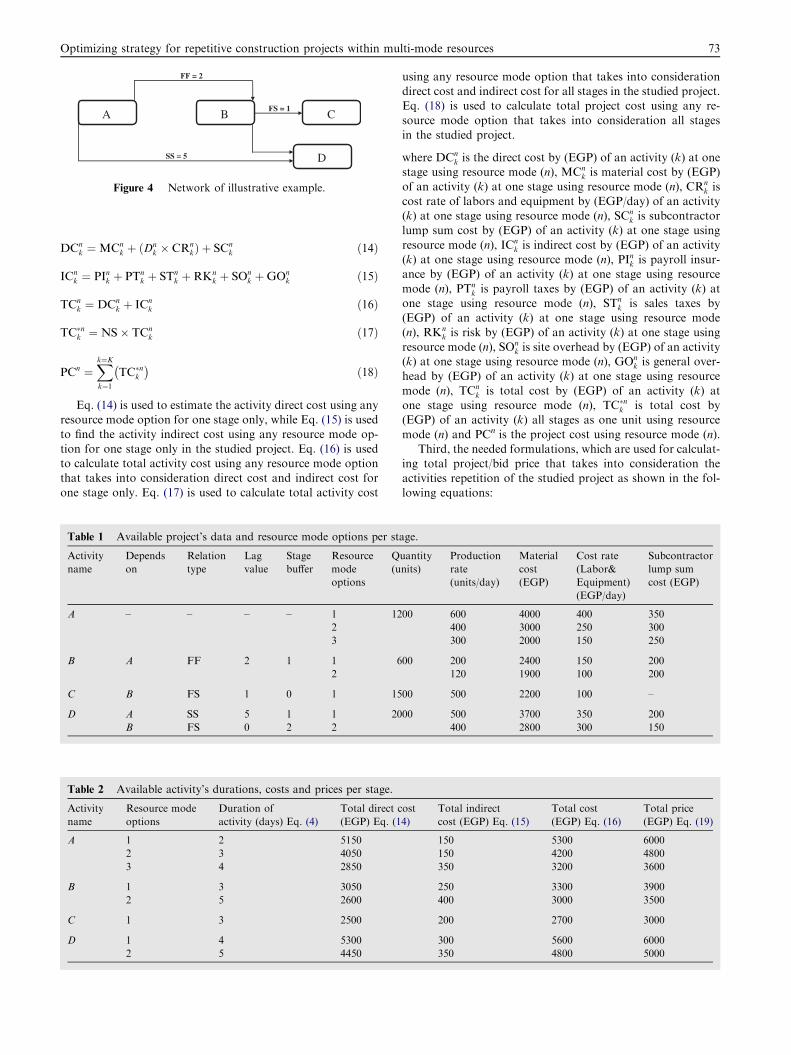
A C B

D

Figure 4 Network of illustrative example.

Optimizing strategy for repetitive construction projects within multi-mode resources 73

DCnk ¼MCn

k þ ðDnk � CRn

kÞ þ SCnk ð14Þ

ICnk ¼ PInk þ PTn

k þ STnk þRKn

k þ SOnk þGOn

k ð15Þ

TCnk ¼ DCn

k þ ICnk ð16Þ

TC�nk ¼ NS� TCnk ð17Þ

PCn ¼Xk¼Kk¼1

TC�nk� �

ð18Þ

Eq. (14) is used to estimate the activity direct cost using anyresource mode option for one stage only, while Eq. (15) is usedto find the activity indirect cost using any resource mode op-

tion for one stage only in the studied project. Eq. (16) is usedto calculate total activity cost using any resource mode optionthat takes into consideration direct cost and indirect cost for

one stage only. Eq. (17) is used to calculate total activity cost

Table 1 Available project’s data and resource mode options per st

Activity

name

Depends

on

Relation

type

Lag

value

Stage

buffer

Resource

mode

options

Q

(u

A – – – – 1 12

2

3

B A FF 2 1 1 6

2

C B FS 1 0 1 15

D A SS 5 1 1 20

B FS 0 2 2

Table 2 Available activity’s durations, costs and prices per stage.

Activity

name

Resource mode

options

Duration of

activity (days) Eq. (4)

Total direct c

(EGP) Eq. (1

A 1 2 5150

2 3 4050

3 4 2850

B 1 3 3050

2 5 2600

C 1 3 2500

D 1 4 5300

2 5 4450

using any resource mode option that takes into considerationdirect cost and indirect cost for all stages in the studied project.Eq. (18) is used to calculate total project cost using any re-

source mode option that takes into consideration all stagesin the studied project.

where DCnk is the direct cost by (EGP) of an activity (k) at one

stage using resource mode (n), MCnk is material cost by (EGP)

of an activity (k) at one stage using resource mode (n), CRnk is

cost rate of labors and equipment by (EGP/day) of an activity(k) at one stage using resource mode (n), SCn

k is subcontractorlump sum cost by (EGP) of an activity (k) at one stage using

resource mode (n), ICnk is indirect cost by (EGP) of an activity

(k) at one stage using resource mode (n), PInk is payroll insur-ance by (EGP) of an activity (k) at one stage using resource

mode (n), PTnk is payroll taxes by (EGP) of an activity (k) at

one stage using resource mode (n), STnk is sales taxes by

(EGP) of an activity (k) at one stage using resource mode(n), RKn

k is risk by (EGP) of an activity (k) at one stage using

resource mode (n), SOnk is site overhead by (EGP) of an activity

(k) at one stage using resource mode (n), GOnk is general over-

head by (EGP) of an activity (k) at one stage using resource

mode (n), TCnk is total cost by (EGP) of an activity (k) at

one stage using resource mode (n), TC�nk is total cost by(EGP) of an activity (k) all stages as one unit using resource

mode (n) and PCn is the project cost using resource mode (n).Third, the needed formulations, which are used for calculat-

ing total project/bid price that takes into consideration the

activities repetition of the studied project as shown in the fol-lowing equations:

age.

uantity

nits)

Production

rate

(units/day)

Material

cost

(EGP)

Cost rate

(Labor&

Equipment)

(EGP/day)

Subcontractor

lump sum

cost (EGP)

00 600 4000 400 350

400 3000 250 300

300 2000 150 250

00 200 2400 150 200

120 1900 100 200

00 500 2200 100 –

00 500 3700 350 200

400 2800 300 150

ost

4)

Total indirect

cost (EGP) Eq. (15)

Total cost

(EGP) Eq. (16)

Total price

(EGP) Eq. (19)

150 5300 6000

150 4200 4800

350 3200 3600

250 3300 3900

400 3000 3500

200 2700 3000

300 5600 6000

350 4800 5000

Table 4 Available project’s solutions using all resource mode

options.

Solution no. Eq. (22) Combination of all resource mode options

01 A1 & B1 & C1 & D1

02 A2 & B1 & C1 & D1

03 A3 & B1 & C1 & D1

04 A1 & B2 & C1 & D1

05 A2 & B2 & C1 & D1

06 A3 & B2 & C1 & D1

07 A1 & B1 & C1 & D2

08 A2 & B1 & C1 & D2

09 A3 & B1 & C1 & D2

10 A1 & B2 & C1 & D2

11 A2 & B2 & C1 & D2

12 A3 & B2 & C1 & D2

Table 5 Main project’s solutions (duration, cost and price)

using all resource mode options.

Solution

no. Eq. (22)

Project duration

(days) Eq. (6)

Project cost

(EGP) Eq. (18)

Project price

(EGP) Eq. (21)

01 48 169,000 189,000

02 49 158,000 177,000

03 58 148,000 165,000

04 59 166,000 185,000

05 60 155,000 173,000

06 61 145,000 161,000

07 58 161,000 179,000

08 59 150,000 167,000

09 68 140,000 155,000

10 62 158,000 175,000

11 63 147,000 163,000

12 64 137,000 151,000

Table 3 Available activity’s durations, costs and prices per project.

Activity name Resource mode

options

Duration of activity

(days) Eq. (5)

Total cost

(EGP) Eq. (17)

Total price

(EGP) Eq. (20)

A 1 20 53,000 60,000

2 30 42,000 48,000

3 40 32,000 36,000

B 1 30 33,000 39,000

2 50 30,000 35,000

C 1 30 27,000 30,000

D 1 40 56,000 60,000

2 50 48,000 50,000

74 Remon Fayek Aziz

TPnk ¼ TCn

k þ POnk ð19Þ

TP�nk ¼ NS� TPnk ð20Þ

PPn ¼Xk¼Kk¼1

TP�nk� �

ð21Þ

Eq. (19) is used to estimate the activity price using any re-source mode option for one stage only, while Eq. (20) is used

to find the activity price using any resource mode option thattakes into consideration all stages in the studied project. Eq.(18) is used to calculate total project/bid price using any re-source mode option that takes into consideration all stages

in the studied project.

where TPnk is the total price by (EGP) of an activity (k) at one

stage using resource mode (n), POnk is profit by (EGP) of an

activity (k) at one stage using resource mode (n), TP�nk is totalprice by (EGP) of an activity (k) at all stages as one unit using

resource mode (n) and PPn is the project/bid price using re-source mode (n).

Fourth, the needed formulations, which are used for calcu-

lating project main solutions and total project sub-solutionsthat takes into consideration the activities repetition of thestudied project as shown in the Eqs. (22) and (23).

TS ¼Yk¼Kk¼1

TOkð Þ ð22Þ

TS� ¼Yk¼Kk¼1

TFk þ 1ð Þ ð23Þ

where TS is the total main solutions of the project using re-

source mode (n), TOk is total options of the activity (k), TS\

is total sub-solutions at any project main-solution using re-source mode (n) and TFk is the total float of the activity (k)

at any project main-solution using resource mode (n).Fifth, the needed formulation that is used for calculating

project maximum working capital that takes into consider-ation the activities repetition of the studied project as shown

in the Eq. (24).

MCn ¼Max:ðNC�OCÞ ð24Þ

where MCn is the maximum working capital along cash flow ofproject sub-solution at any project main-solution using re-

source mode (n), NC is sum the in cash flows before receivingthe invoice value at any time period in the project and OC isthe sum the out cash flows at any time period in the project.

Sixth, the needed formulation that is used for calculating

project net present value that takes into consideration theactivities repetition of the studied project as shown in theEq. (25).

NPn ¼ F

ð1þ i=365Þm ð25Þ

whereNPn is the net present value at the beginning of the project

that is equivalent to net profit of project sub-solution at any pro-ject main-solution using resource mode (n), F is differencebetween daily price and daily cost at any time of project

Table 6 Total project’s solutions using all resource mode options with available activities start times.

Main sol.

no. Eq. (22)

Sub. sol.

no. Eq. (23)

Sol. ID PD (days)

Eq. (6)

PC (EGP)

Eq. (18)

PP (EGP)

Eq. (21)

Selected start time of activity. Check network

logic

MC Eq. (24) NP Inves = 10%,

Loan = 14%, Eq. (25)

NP Inves = 14%,

Loan = 14%, Eq. (25)A B C D

01 01 01 48 169,000 189,000 0 2 6 8 Valid 40,250.0 19,922.7 19,454.2

01 02 02 48 169,000 189,000 0 2 7 8 Valid 40,250.0 19,925.1 19,452.5

01 03 03 48 169,000 189,000 0 2 8 8 Valid 39,350.0 19,928.5 19,453.2

01 04 04 48 169,000 189,000 0 2 9 8 Valid 38,460.0 19,931.9 19,453.9

01 05 05 48 169,000 189,000 0 2 10 8 Valid 38,460.0 19,935.3 19,454.6

01 06 06 48 169,000 189,000 0 2 11 8 Valid 38,460.0 19,938.7 19,455.3

01 07 07 48 169,000 189,000 0 2 12 8 Valid 38,460.0 19,938.0 19,456.0

01 08 08 48 169,000 189,000 0 2 13 8 Valid 38,460.0 19,939.7 19,454.3

01 09 09 48 169,000 189,000 0 2 14 8 Valid 38,460.0 19,942.8 19,452.6

01 10 10 48 169,000 189,000 0 2 15 8 Valid 37,560.0 19,946.2 19,453.3

01 11 11 48 169,000 189,000 0 2 16 8 Valid 36,660.0 19,949.6 19,454.0

01 12 12 48 169,000 189,000 0 2 17 8 Valid 35,760.0 19,953.0 19,454.7

01 13 13 48 169,000 189,000 0 2 18 8 Valid 34,860.0 19,956.3 19,455.4

02 01 14 49 158,000 177,000 0 3 7 9 Valid 32,520.0 18,958.2 18,488.0

02 02 15 49 158,000 177,000 0 3 8 9 Valid 32,520.0 18,961.7 18,488.7

02 03 16 49 158,000 177,000 0 3 9 9 Valid 32,520.0 18,965.1 18,489.4

02 04 17 49 158,000 177,000 0 3 10 9 Valid 32,520.0 18,968.5 18,490.1

02 05 18 49 158,000 177,000 0 3 11 9 Valid 32,520.0 18,971.9 18,490.8

02 06 19 49 158,000 177,000 0 3 12 9 Valid 32,520.0 18,971.2 18,491.5

02 07 20 49 158,000 177,000 0 3 13 9 Valid 32,520.0 18,972.9 18,489.8

02 08 21 49 158,000 177,000 0 3 14 9 Valid 32,520.0 18,975.9 18,488.1

02 09 22 49 158,000 177,000 0 3 15 9 Valid 32,100.0 18,979.3 18,488.8

02 10 23 49 158,000 177,000 0 3 16 9 Valid 32,100.0 18,982.7 18,489.5

02 11 24 49 158,000 177,000 0 3 17 9 Valid 32,100.0 18,986.1 18,490.2

02 12 25 49 158,000 177,000 0 3 18 9 Valid 32,100.0 18,989.5 18,490.9

02 13 26 49 158,000 177,000 0 3 19 9 Valid 32,100.0 18,988.1 18,491.6

03 01 27 58 148,000 165,000 0 12 16 18 Valid 28,710.0 17,022.1 16,442.4

03 02 28 58 148,000 165,000 0 12 17 18 Valid 28,710.0 17,025.4 16,443.1

03 03 29 58 148,000 165,000 0 12 18 18 Valid 28,710.0 17,028.8 16,443.8

03 04 30 58 148,000 165,000 0 12 19 18 Valid 28,710.0 17,027.5 16,444.5

03 05 31 58 148,000 165,000 0 12 20 18 Valid 28,710.0 17,029.1 16,442.8

03 06 32 58 148,000 165,000 0 12 12 18 Valid 28,710.0 17,032.9 16,441.1

03 07 33 58 148,000 165,000 0 12 22 18 Valid 28,500.0 17,036.3 16,441.8

03 08 34 58 148,000 165,000 0 12 23 18 Valid 28,500.0 17,039.6 16,442.5

03 09 35 58 148,000 165,000 0 12 24 18 Valid 28,500.0 17,043.0 16,443.2

03 10 36 58 148,000 165,000 0 12 25 18 Valid 28,500.0 17,046.4 16,443.9

03 11 37 58 148,000 165,000 0 12 26 18 Valid 28,500.0 17,044.3 16,444.6

03 12 38 58 148,000 165,000 0 12 27 18 Valid 28,500.0 17,046.0 16,442.9

03 13 39 58 148,000 165,000 0 12 28 18 Valid 28,500.0 17,050.4 16,441.2

04 01 40 59 166,000 185,000 0 2 26 19 Valid 22,250.0 18,989.5 18,377.2

04 02 41 59 166,000 185,000 0 2 27 19 Valid 22,250.0 18,991.1 18,375.5

04 03 42 59 166,000 185,000 0 2 28 19 Valid 22,250.0 18,995.5 18,373.9

04 04 43 59 166,000 185,000 0 2 29 19 Valid 22,250.0 18,998.9 18,374.6

Optim

izingstra

tegyforrep

etitiveconstru

ctionprojects

with

inmulti-m

odereso

urces

75

Table 6 (continued)

Main sol.

no. Eq. (22)

Sub. sol.

no. Eq. (23)

Sol. ID PD (days)

Eq. (6)

PC (EGP)

Eq. (18)

PP (EGP)

Eq. (21)

Selected start time of activity. Check network

logic

MC Eq. (24) NP Inves = 10%,

Loan = 14%, Eq. (25)

NP Inves = 14%,

Loan = 14%, Eq. (25)A B C D

05 01 44 60 155,000 173,000 0 3 27 20 Valid 23,370.0 18,033.0 17,413.4

05 02 45 60 155,000 173,000 0 3 28 20 Valid 22,470.0 18,037.4 17,411.7

05 03 46 60 155,000 173,000 0 3 29 20 Valid 22,470.0 18,040.7 17,412.4

05 04 47 60 155,000 173,000 0 3 30 20 Valid 22,470.0 18,044.1 17,413.1

06 01 48 61 145,000 161,000 0 4 28 21 Valid 25,250.0 16,084.4 15,457.3

06 02 49 61 145,000 161,000 0 4 29 21 Valid 24,350.0 16,087.7 15,458.0

06 03 50 61 145,000 161,000 0 4 30 21 Valid 23,720.0 16,091.1 15,458.7

06 04 51 61 145,000 161,000 0 4 31 21 Valid 23,720.0 16,094.5 15,459.4

07 01 52 58 161,000 179,000 0 2 6 8 Valid 37,610.0 17,883.9 17,404.9

07 02 53 58 161,000 179,000 0 2 7 8 Valid 37,610.0 17,886.3 17,403.2

07 03 54 58 161,000 179,000 0 2 8 8 Valid 36,710.0 17,889.7 17,403.9

07 04 55 58 161,000 179,000 0 2 9 8 Valid 35,810.0 17,893.1 17,404.6

07 05 56 58 161,000 179,000 0 2 10 8 Valid 35,440.0 17,896.5 17,405.3

07 06 57 58 161,000 179,000 0 2 11 8 Valid 35,440.0 17,899.9 17,406.0

07 07 58 58 161,000 179,000 0 2 12 8 Valid 35,440.0 17,899.2 17,406.7

07 08 59 58 161,000 179,000 0 2 13 8 Valid 35,440.0 17,900.9 17,405.0

07 09 60 58 161,000 179,000 0 2 14 8 Valid 35,440.0 17,904.0 17,403.3

07 10 61 58 161,000 179,000 0 2 15 8 Valid 34,540.0 17,907.4 17,404.0

07 11 62 58 161,000 179,000 0 2 16 8 Valid 33,640.0 17,910.8 17,404.7

07 12 63 58 161,000 179,000 0 2 17 8 Valid 32,740.0 17,914.2 17,405.4

07 13 64 58 161,000 179,000 0 2 18 8 Valid 31,840.0 17,917.6 17,406.1

07 14 65 58 161,000 179,000 0 2 19 8 Valid 31,310.0 17,916.2 17,406.8

07 15 66 58 161,000 179,000 0 2 20 8 Valid 31,310.0 17,917.9 17,405.1

07 16 67 58 161,000 179,000 0 2 21 8 Valid 31,310.0 17,921.6 17,403.4

07 17 68 58 161,000 179,000 0 2 22 8 Valid 31,310.0 17,925.0 17,404.1

07 18 69 58 161,000 179,000 0 2 23 8 Valid 31,310.0 17,928.4 17,404.8

07 19 70 58 161,000 179,000 0 2 24 8 Valid 31,310.0 17,931.7 17,405.5

07 20 71 58 161,000 179,000 0 2 25 8 Valid 31,310.0 17,935.1 17,406.2

07 21 72 58 161,000 179,000 0 2 26 8 Valid 31,310.0 17,933.1 17,406.9

07 22 73 58 161,000 179,000 0 2 27 8 Valid 31,310.0 17,934.7 17,405.2

07 23 74 58 161,000 179,000 0 2 28 8 Valid 31,310.0 17,939.1 17,403.5

08 01 75 59 150,000 167,000 0 3 7 9 Valid 29,490.0 16,929.2 16,443.2

08 02 76 59 150,000 167,000 0 3 8 9 Valid 29,490.0 16,932.6 16,443.9

08 03 77 59 150,000 167,000 0 3 9 9 Valid 29,490.0 16,936.0 16,444.6

08 04 78 59 150,000 167,000 0 3 10 9 Valid 29,490.0 16,939.4 16,445.3

08 05 79 59 150,000 167,000 0 3 11 9 Valid 29,490.0 16,942.8 16,446.0

08 06 80 59 150,000 167,000 0 3 12 9 Valid 29,490.0 16,942.1 16,446.7

08 07 81 59 150,000 167,000 0 3 13 9 Valid 29,490.0 16,943.8 16,445.0

08 08 82 59 150,000 167,000 0 3 14 9 Valid 29,490.0 16,946.9 16,443.3

08 09 83 59 150,000 167,000 0 3 15 9 Valid 29,490.0 16,950.3 16,444.0

08 10 84 59 150,000 167,000 0 3 16 9 Valid 29,490.0 16,953.7 16,444.7

08 11 85 59 150,000 167,000 0 3 17 9 Valid 29,490.0 16,957.1 16,445.4

08 12 86 59 150,000 167,000 0 3 18 9 Valid 29,490.0 16,960.5 16,446.1

08 13 87 59 150,000 167,000 0 3 19 9 Valid 29,490.0 16,959.1 16,446.8

08 14 88 59 150,000 167,000 0 3 20 9 Valid 29,490.0 16,960.8 16,445.1

08 15 89 59 150,000 167,000 0 3 21 9 Valid 29,490.0 16,964.5 16,443.4

08 16 90 59 150,000 167,000 0 3 22 9 Valid 28,240.0 16,967.9 16,444.1

76

Rem

onFayek

Aziz

08 17 91 59 150,000 167,000 0 3 23 9 Valid 27,340.0 16,971.3 16,444.8

08 18 92 59 150,000 167,000 0 3 24 9 Valid 26,440.0 16,974.6 16,445.5

08 19 93 59 150,000 167,000 0 3 25 9 Valid 25,540.0 16,978.0 16,446.2

08 20 94 59 150,000 167,000 0 3 26 9 Valid 24,640.0 16,976.0 16,446.9

08 21 95 59 150,000 167,000 0 3 27 9 Valid 23,740.0 16,977.6 16,445.2

08 22 96 59 150,000 167,000 0 3 28 9 Valid 23,190.0 16,982.0 16,443.5

08 23 97 59 150,000 167,000 0 3 29 9 Valid 23,190.0 16,985.4 16,444.2

09 01 98 68 140,000 155,000 0 12 16 18 Valid 25,660.0 15,028.4 14,456.2

09 02 99 68 140,000 155,000 0 12 17 18 Valid 25,660.0 15,031.8 14,456.8

09 03 100 68 140,000 155,000 0 12 18 18 Valid 25,660.0 15,035.2 14,457.5

09 04 101 68 140,000 155,000 0 12 19 18 Valid 25,660.0 15,033.8 14,458.2

09 05 102 68 140,000 155,000 0 12 20 18 Valid 25,660.0 15,035.5 14,456.5

09 06 103 68 140,000 155,000 0 12 21 18 Valid 25,660.0 15,039.3 14,454.8

09 07 104 68 140,000 155,000 0 12 22 18 Valid 25,520.0 15,042.6 14,455.5

09 08 105 68 140,000 155,000 0 12 23 18 Valid 25,520.0 15,046.0 14,456.2

09 09 106 68 140,000 155,000 0 12 24 18 Valid 25,520.0 15,049.4 14,456.9

09 10 107 68 140,000 155,000 0 12 25 18 Valid 25,520.0 15,052.8 14,457.6

09 11 108 68 140,000 155,000 0 12 26 18 Valid 25,520.0 15,050.7 14,458.3

09 12 109 68 140,000 155,000 0 12 27 18 Valid 25,520.0 15,052.4 14,456.6

09 13 110 68 140,000 155,000 0 12 28 18 Valid 25,520.0 15,056.8 14,454.9

09 14 111 68 140,000 155,000 0 12 29 18 Valid 24,620.0 15,060.1 14,455.6

09 15 112 68 140,000 155,000 0 12 30 18 Valid 23,780.0 15,063.5 14,456.3

09 16 113 68 140,000 155,000 0 12 31 18 Valid 23,780.0 15,066.9 14,457.0

09 17 114 68 140,000 155,000 0 12 32 18 Valid 23,780.0 15,070.2 14,457.7

09 18 115 68 140,000 155,000 0 12 33 18 Valid 23,780.0 15,067.5 14,458.4

09 19 116 68 140,000 155,000 0 12 34 18 Valid 23,780.0 15,069.2 14,456.7

09 20 117 68 140,000 155,000 0 12 35 18 Valid 23,780.0 15,074.2 14,455.0

09 21 118 68 140,000 155,000 0 12 36 18 Valid 22,880.0 15,077.6 14,455.7

09 22 119 68 140,000 155,000 0 12 37 18 Valid 21,980.0 15,080.9 14,456.4

09 23 120 68 140,000 155,000 0 12 38 18 Valid 21,080.0 15,084.3 14,457.1

10 01 121 62 158,000 175,000 0 2 26 12 Valid 25,880.0 16,988.8 16,425.2

10 02 122 62 158,000 175,000 0 2 27 12 Valid 25,880.0 16,990.5 16,423.5

10 03 123 62 158,000 175,000 0 2 28 12 Valid 25,880.0 16,994.9 16,421.8

10 04 124 62 158,000 175,000 0 2 29 12 Valid 25,880.0 16,998.3 16,422.5

10 05 125 62 158,000 175,000 0 2 30 12 Valid 25,880.0 17,001.6 16,423.2

10 06 126 62 158,000 175,000 0 2 31 12 Valid 25,880.0 17,005.0 16,423.9

10 07 127 62 158,000 175,000 0 2 32 12 Valid 25,880.0 17,008.4 16,424.6

11 01 128 63 147,000 163,000 0 3 27 13 Valid 20,720.0 16,026.2 15,463.0

11 02 129 63 147,000 163,000 0 3 28 13 Valid 19,890.0 16,030.6 15,461.3

11 03 130 63 147,000 163,000 0 3 29 13 Valid 19,890.0 16,034.0 15,462.0

11 04 131 63 147,000 163,000 0 3 30 13 Valid 19,890.0 16,037.4 15,462.7

11 05 132 63 147,000 163,000 0 3 31 13 Valid 19,890.0 16,040.7 15,463.4

11 06 133 63 147,000 163,000 0 3 32 13 Valid 19,890.0 16,044.1 15,464.1

11 07 134 63 147,000 163,000 0 3 33 13 Valid 19,890.0 16,041.4 15,464.8

12 01 135 64 137,000 151,000 0 4 28 14 Valid 22,660.0 14,046.2 13,466.9

12 02 136 64 137,000 151,000 0 4 29 14 Valid 21,760.0 14,049.6 13,467.6

12 03 137 64 137,000 151,000 0 4 30 14 Valid 21,200.0 14,052.9 13,468.2

12 04 138 64 137,000 151,000 0 4 31 14 Valid 21,200.0 14,056.3 13,468.9

12 05 139 64 137,000 151,000 0 4 32 14 Valid 21,200.0 14,059.6 13,469.6

12 06 140 64 137,000 151,000 0 4 33 14 Valid 21,200.0 14,056.9 13,470.3

12 07 141 64 137,000 151,000 0 4 34 14 Valid 21,200.0 14,058.6 13,468.6

Optim

izingstra

tegyforrep

etitiveconstru

ctionprojects

with

inmulti-m

odereso

urces

77

orking

Net

present

valueInves

=10%,

Loan=

14%

Min.multi-objective

fitnessEq.(26)

Rem

arks

019,956.3

0.00000

W1=

1.0

014,059.6

0.00000

W2=

1.0

016,044.1

0.00000

W3=

1.0

019,956.3

�1.00000

W4=

1.0

018,989.5

0.36711

W1&

W2=

1/2

018,989.5

0.32485

W1&

W3=

1/2

019,956.3

�0.50000

W1&

W4=

1/2

014,059.6

0.03217

W2&

W3=

1/2

018,989.5

�0.07610

W2&

W4=

1/2

018,998.9

�0.36105

W3&

W4=

1/2

014,059.6

0.28811

W1&

W2&

W3=

1/3

018,989.5

�0.03407

W1&

W2&

W4=

1/3

019,956.3

�0.08824

W1&

W3&

W4=

1/3

016,044.1

�0.00742

W2&

W3&

W4=

1/3

018,989.5

0.12438

W1&

W2&

W3&

W4=

1/4

78 Remon Fayek Aziz

sub-solution at any project main-solution using resource mode

(n), i is investment rate per year in case of positive F or loan rateper year in case of negative and m is the time period per days.

Finally, the needed multi-objective formulation that is used

for optimizing between project solutions that takes into con-sideration the activities repetition of the studied project asshown in the Eq. (26).

Zn ¼W1 � PDn � PDmin

PDmax�PDminþW2 � PPn � PPmin

PPmax�PPmin

þW3 � MCn �MCmin

MCmax�MCminþW4

� NPmin�NPn

NPmax�NPminð26Þ

W1þW2þW3þW4 ¼ 1:0 ð27Þ

where Zn is the multi-objective fitness formula for project sub-

solution (time; price; capital and profit) at any project main-solution using resource mode (n), W1; W2; W3 and W4 isweights of all terms for fitness formula, PDmin is the minimum

of project duration of all solutions, PDmax is the maximum ofproject duration of all solutions, PPmin is the minimum of pro-ject price ‘‘bid price’’ of all solutions, PPmax is the maximum of

project duration of all solutions, MCmin is the minimum ofproject maximum working capital of all solutions, MCmax isthe maximum of project maximum working capital of all solu-

tions, NPmin is the minimum of project net present value of allsolutions and NPmax is the maximum of project net present va-lue of all solutions.

Table

7First

solutionofallscenariosin

case

ofinvestm

entrate

10%

andloanrate

14%

.

Main

sol.no.

Sub.

sol.no.

Sol.

ID

Project

duration

(days)

Project

price

(EGP)

Start

timeofactivity

Max.w

capital

AB

CD

01

13

013

48

189,000.0

02

18

08

34,860.

12

05

139

64

151,000.0

04

32

14

21,200.

11

06

133

63

163,000.0

03

32

13

19,890.

01

13

013

48

189,000.0

02

18

08

34,860.

02

12

025

49

177,000.0

03

18

09

32,100.

02

12

025

49

177,000.0

03

18

09

32,100.

01

13

013

48

189,000.0

02

18

08

34,860.

12

05

139

64

151,000.0

04

32

14

21,200.

02

12

025

49

177,000.0

03

18

09

32,100.

04

04

043

59

185,000.0

02

29

19

22,250.

12

05

139

64

151,000.0

04

32

14

21,200.

02

12

025

49

177,000.0

03

18

09

32,100.

01

13

013

48

189,000.0

02

18

08

34,860.

11

06

133

63

163,000.0

03

32

13

19,890.

02

12

025

49

177,000.0

03

18

09

32,100.

10. Illustrative example

This section presents the results of practical multi-objectiveoptimization formulations that are used for selecting optimal

repetitive project solutions. The main objective of these results,of present system, is to provide fixed small solutions for typi-cal-repetitive construction projects as contractor needs to opti-

mize resource utilization modes for giving the best tenderingoffer in order to simultaneously minimize project duration,project/bid price and project maximum working capital while

maximizing its net present value. To accomplish these, formu-las are used in illustrative example to provide a number of newand unique capabilities, including: (1) Ranking the obtained

optimal plans according to a set of specified weights that rep-resents the relative importance of project duration, project/bidprice, project maximum working capital and project net pres-ent value in the analyzed repetitive construction project solu-

tions; (2) Visualizing and viewing the generated optimaltrade-off among construction project duration, project/bidprice, project maximum working capital and project net pres-

ent value to facilitate the selection of an optimal plan that con-siders the specific project needs; and (3) Providing seamlessintegration with available project management calculations

and runs, to benefit from their practical project schedulingand control features. Input data for one stage of illustrativeexample are shown in Fig. 4 and Tables 1–3, project consistsof four activities with different relationships among them as

shown in Fig. 4 and Table 1. These activities have variousnumber of resource mode options, each mode has its own pro-duction rate (units/day), material cost (EGP), cost rate (la-

bor& equipment) (EGP/day) and subcontractor lump sum

Table

8First

solutionofallscenariosin

case

ofinvestm

entrate

14%

andloanrate

14%

.

Main

sol.no.

Sub.

sol.no.

Sol.

ID

Project

d

uration

(days)

Project

price

(EGP)

Start

timeofactivity

Max.working

capital

Net

present

valueInves

=14%

Loan=

14%

Min.multi-objective

fitnessEq.(26)

Rem

arks

AB

CD

01

13

013

48

189,000.0

02

18

08

34,860.0

19,455.4

0.00000

W1=

1.0

12

06

140

64

151,000.0

04

33

14

21,200.0

13,470.3

0.00000

W2=

1.0

11

07

134

63

163,000.0

03

33

13

19,890.0

15,464.8

0.00000

W3=

1.0

01

07

007

48

189,000.0

02

12

08

38,460.0

19,456.0

�1.00000

W4=

1.0

02

13

026

49

177,000.0

03

19

09

32,100.0

18,491.6

0.36711

W1&

W2=

1/2

02

13

026

49

177,000.0

03

19

09

32,100.0

18,491.6

0.32485

W1&

W3=

1/2

01

07

007

48

189,000.0

02

12

08

38,460.0

19,456.0

�0.50000

W1&

W4=

1/2

12

06

140

64

151,000.0

04

33

14

21,200.0

13,470.3

0.03217

W2&

W3=

1/2

02

13

026

49

177,000.0

03

19

09

32,100.0

18,491.6

�0.07738

W2&

W4=

1/2

04

01

040

59

185,000.0

02

26

19

22,250.0

18,377.2

�0.35198

W3&

W4=

1/2

12

06

140

64

151,000.0

04

33

14

21,200.0

13,470.3

0.28811

W1&

W2&

W3=

1/3

02

13

026

49

177,000.0

03

19

09

32,100.0

18,491.6

�0.03492

W1&

W2&

W4=

1/3

01

13

013

48

189,000.0

02

18

08

34,860.0

19,956.3

�0.08821

W1&

W3&

W4=

1/3

11

07

134

63

163,000.0

03

33

13

19,890.0

15,464.8

�0.00593

W2&

W3&

W4=

1/3

02

13

026

49

177,000.0

03

19

09

32,100.0

18,491.6

0.12374

W1&

W2&

W3&

W4=

1/4

Optimizing strategy for repetitive construction projects within multi-mode resources 79

cost (EGP) as shown in Table 1. After applying previous for-mulas, Table 2 shows the activities data (duration with corre-sponding cost and price) for each resource mode option taking

into consideration one stage of studied example. Table 3 showsthe activities data (duration with corresponding cost and price)for each resource mode option taking into consideration all

stages of studied example. Number of repetitive stages of ana-lyzed example equal to ten typical stages.

By applying Eq. (22), Table 4 shows the number of possible

main solutions according to activities resource modes combi-nation of analyzed example. Table 5 shows available main pro-ject solutions (duration with corresponding cost and price) foreach resource mode option taking into consideration all stages

of studied example.Table 6 shows available project sub-solutions (duration

with corresponding cost, price, maximum working capital

and net present value) for each resource mode option takinginto consideration all stages of studied example.

After applying multi-objective optimization formula as

mentioned in Eq. (26), Tables 7 and 8 give the first result ofoptimal ranked solutions for each scenario from total fifteenscenarios.

11. Conclusion

This paper presented the development of a multi-objective opti-

mization formulation in order to search the optimal project ten-der offer in the typical repetitive construction project withinmulti-mode resource options for all activities, which minimizeproject duration, project/bid price and project maximum work-

ing capital while maximizing its net present value simulta-neously. It was developed in two main tasks: First task, theformulation was designed to incorporate and enable the opti-

mization of any repetitive project. Second task, the formulationwas designed to enable available starting times for all activitiesin the project and select the suitable start time of each activity

within the total float to get best optimization scenario. Anapplication example was analyzed to illustrate the use of formu-lations and demonstrate its optimization process and develop-

ing minimum financing construction with scheduling. Thesenew capabilities should prove its usefulness for contractors inrepetitive construction projects, especially those who are in-volved in new types of contracts that minimize tender data.

References

[1] W. Yu, K. Wang, M. Wang, Pricing Strategy for Best Value

Tender, Journal of Construction Engineering and Management,

Posted ahead of print 31 August 2012, http://dx.doi.org/

10.1061/(ASCE)CO.1943-7862.0000635.

[2] S. Peer, Application of cost flow forecasting models, Journal of

the Construction Division ASCE 108 (CO2) (1982) 226–232.

[3] S. Singh, G. Lakanathan, Computer-based cash flow model, in:

Proceedings of the 36th Annual Transactions of the American

Association of Cost Engineers – AACE, AACE, WV, USA,

1992, No. R.5.1–R.5.14.

[4] R. Navon, Resource-based model for automatic cash flow

forecasting, Construction Management and Economics 13 (6)

(1995) 501–510.

[5] A. Boussabaine, A. Kaka, A neural networks approach for cost

flow forecasting, Construction Management and Economics 16

(4) (1998) 471–479.

80 Remon Fayek Aziz

[6] R. Calvert, Introduction to Building Management, fifth ed.,

Butterworts, London, 1986.

[7] F. Harris, R. McCaffer, Modern Construction Management,

fifth ed., Blackwell Science, Oxford, Great Britain, 2001.

[8] R. McCaffer, Cash flow forecasting, Quantity Surveying (1979)

22–26.

[9] A. Kaka, A. Boussabaine, Updating techniques for cumulative

cost forecasting on construction projects, Journal of

Construction Procurement. 5 (2) (1999) 141–158.

[10] R. Kenley, ‘‘In-project end-date forecasting: an idiographic,

deterministic approach, using cash flow modeling, Journal

Financial Management of Property and Construction 6 (3)

(2001) 209–216.

[11] R. Kenley, Financing Construction: Cash Flows and Cash

Farming, Spon, London, 2003.

[12] F. Khosrowshahi, A radical approach to risk in project financial

management, in: A. Akintoye (Ed.), Procs 16th Annual

ARCOM Conference, Glasgow Caledonian University, 2000

(September 6–8), pp. 547–556.

[13] D. Cormican, Construction Management: Planning and

Finance, Longman Group Ltd., London, 1985.

[14] B. Cooke, W. Jepson, Cost and Financial Control for

Construction Firms, Macmillan Educational Ltd., London,

1986, pp. 25–26, 41–46.

[15] H. Odeyinka, J. Lowe, An evaluation of methodological issues

for assessing risk impacts on construction cash flow forecast, in:

A. Akintoye (Ed.), Procs 17th Annual ARCOM Conference,

University of Salford, 2001 (September 5–7), pp. 381–389.

[16] A. Kaka, A. Price, Modeling standard cost commitment curves

for contractors’ cash flow forecasting, Construction

Management and Economics 11 (4) (1993) 271–283.

[17] M. Mawdesley, W. Askew, M. O’Reilly, Planning and

Controlling Construction Projects: The Best Laid Plans,

Addison Wesley Longman and The Chartered Institute of

Building, Essex, 1997, pp. 42-45, 64-67.

[18] J. Lowe, Cash flow and the construction client: a theoretical

approach, in: P. Lansley, P. Harlow (Eds.), Managing

Construction Worldwide, vol. 1, Spon, London, 1987, pp. 27–

336.

[19] Q. Cui, M. Hastak, D. Halpin, Systems analysis of project cash

flow management strategies, Construction Management and

Economics 28 (4) (2010) 361–376.

[20] A. Senouci, K. El-Rayes, Time-profit trade-off analysis for

construction projects, Journal of Construction Engineering and

Management 135 (8) (2009) 718–725.

[21] A. Elazouni, F. Metwally, Finance-based scheduling: Tool to

maximize project profit using improved genetic algorithms,

Journal of Construction Engineering and Management 131 (4)

(2005) 400–412.

[22] A. Elazouni, F. Metwally, Expanding finance-based scheduling

to devise overall-optimized project schedules, Journal of

Construction Engineering and Management 133 (1) (2007) 86–

90.

[23] A. Elazouni, Heuristic method for multi-project finance-based

scheduling, Construction Management and Economics 27 (2)

(2009) 199–211.

[24] S. Liu, C. Wang, Resource-constrained construction project

scheduling model for profit maximization considering cash flow,

Automation in Construction 17 (8) (2008) 966–974.

[25] S. Singh, Developing a computer model for cash flow planning,

Cost Engineering 31 (11) (2001) 7–11.

[26] D. Halpin, R. Woodhead, Construction Management, John

Wiley & Sons, NY, 1998.

[27] J. Graham, C. Harvey, The theory and practice of corporate

finance. evidence from the field, Journal Financial Economics 60

(2001) 187–243.

[28] L. Remmers, International financial management: 35 years later-

what has changed?, International Business Review 13 (2004)

155–180.

[29] G. Ryan, P. Ryan, Capital budgeting practices of the Fortune

1000: How have things changed?, Journal Business Manage 8 (4)

(2002) 355–364.

[30] M. Danielson, J. Scott, The capital budgeting decision of small

business, Working paper presented at the FMA 2005 annual

meeting, 2005.

[31] M. Mekonnen, The process of investment appraisal: the

experience of 10 large British and Dutch companies,

International Journal of Project Management 21 (2003) 355–

362.

[32] G. Sandahl, S. Sjogren, Capital budgeting methods among

Sweden’s largest groups of companies: the state of the art and a

comparison with earlier studies, International Journal

Production Economics 84 (2003) 51–69.

[33] G. Lucko, R. Thompson, Derivation and assessment of interest

in cash flow calculations for time-cost optimizations in

construction project management in: Proceedings of the

Winter Simulation Conference, 2010, pp. 3037–3048.

[34] A. Touran, M. Atgun, I. Bhurisith, Analysis of the United States

department of transportation prompt pay provisions, Journal of

Construction Engineering and Management 130 (5) (2004) 719–

725.

[35] F. Khosrowshahi, A. Kaka, A decision support model for

construction cash flow management, Computer-Aided Civil and

Infrastructure Engineering 22 (7) (2007) 527–539.

[36] M. Cheng, Y. Wu, Evolutionary support vector machine

inference system for construction management, Automation in

Construction 18 (5) (2009) 597–604.

[37] M. Cheng, A. Roy, Evolutionary fuzzy decision model for cash

flow prediction using time-dependent support vector machines,

International Journal of Project Management 29 (2011) 56–65.

[38] H. Abdel-Khalek, S. Hafez, A. Lakany, Y. Abuel-Magd,

Financing – scheduling optimization for construction projects

by using genetic algorithms, in: International Conference on

Innovation, Engineering Management and Technology, vol. 59,

World Academy of Science, Engineering and Technology

WASET, Paris, France, 2011, pp. 289–297.

[39] M. Ammar, Optimization of project time-cost trade-off problem

with discounted cash flows, Journal of Construction Engineering

and Management 137 (1) (2011) 65–71.

[40] G. Lucko, optimizing cash flows for linear schedules modeled

with singularity functions by simulated annealing, Journal of

Construction Engineering and Management 137 (7) (2011) 523–

535.

[41] S. Liu, C. Wang, Profit optimization for multiproject scheduling

problems considering cash flow, Journal of Construction

Engineering and Management 136 (12) (2010) 1268–1278.

[42] A. Maravas, J. Pantouvakis, A fuzzy repetitive scheduling

method for projects with repeating activities, Journal of

Construction Engineering and Management 137 (7) (2011)

561–564.

[43] A. Maravas, J. Pantouvakis, Project cash flow analysis in the

presence of uncertainty in activity duration and cost,

International Journal of Project Management 30 (2012) 374–

384.

[44] L. Hong, An empirical examination of project contractors’

supply-chain cash flow performance and owners’ payment

patterns, International Journal of Project Management 29

(2011) 604–614.

[45] R. Oxley, J. Poskitt, Management techniques applied to the

construction industry, fifthth ed., Blackwell Science, London,

1996.

Optimizing strategy for repetitive construction projects within multi-mode resources 81

[46] K. Al-Joburi, R. Al-Aomar, M. Bahri, Analyzing the Impact of

Negative Cash Flow on Construction Performance in the Dubai

Area, Journal of Management in Engineering, Posted ahead of

print 18 February 2012, http://dx.doi.org/10.1061/(ASCE)ME.

1943-5479.0000123.

[47] C. Christenson, Construction of present value tables for use in

evaluation of capital investment opportunities, The Accounting

Review (1955) 666–673.

[48] J. Dean, Measuring the Productivity of Capital, Harvard

Business Review (1954) 120–130.

[49] H. Bierman, S. Smidt, The Capital Budgeting Decision, seventh

ed., McMillan, 1988.

[50] R. Neo, International Construction Contracting, Gower, 1976.

[51] P. Marsh, Contracts and Payment Structures, in: D. Lock, (Ed.),

Project Management Handbook, 1987, pp. 93–118, (Chapter 5).