-1-

OBSERVABILITY AND REDUNDANCY DECOMPOSITION

APPLICATION TO DIAGNOSIS

José Ragot, Didier Maquin and Frédéric Kratz

This paper describes different ways of generating analytical redundancy equations in the case ofsystems represented by either static or dynamic equations. A relation is called a redundancyequation when known variables only, i.e. measured variables or controlled inputs of the system,appear in its expression. Redundancies are a powerful tool for monitoring processes as they can beused to detect and isolate sensor and actuator faults. The classical methods for generatingredundancy equations are presented first. A method using the decomposition of the processequations by the observability concept is also described. The general character of the methods ofgeneration of redundancy equations is demonstrated by showing that the same formalism can beapplied to static and dynamic systems. This general character also appears when redundancyequations are used for detecting faults. Indeed, the statistical tests, presented in this paper, which areused for detecting and localizing the faults, apply indifferently to static and dynamic representations.

1.1 INTRODUCTION

The safety of processes can be greatly enhanced through the detection and isolation of the changesindicative of modifications in the process performances. If the models describing the process areaccurate, the problem of fault detection may be solved by observer-type filters. These filters generatethe so-called residuals computed from the inputs and the outputs of the process. This residualgeneration is the first stage in the problem of fault detection and identification (FDI). For them to beuseful in FDI, the residuals must be insensitive to modelling errors and highly sensitive to thefailures under consideration. In that regard, the residuals are designed so that the effects of possiblefailures are enhanced which in turn increases their detectability. The residuals must also respond

-2-

quickly. The second stage of FDI is concerned with residuals analysis and decision making; theresiduals are examined for detecting the presence of failures. The use of simple decision rules suchas threshold tests or more sophisticated approaches using pattern recognition, sequential probabilityratio test or sensitivity analysis is very helpful at this stage. Various FDI method have been reportedin the literature, notably in the excellent survey papers of Willsky (1976), Iserman (1984), Frank(1990), Gertler (1988 and 1991), Patton (1991). Among the classical books on the subject are thoseof Himmelblau (1978), Pau (1981), Basseville (1986a), Patton (1989b), Dubuisson (1990). Theparticular point of view of data reconciliation is addressed in the book of Ragot (1990a).

This paper is devoted to the generation of residuals using observability analysis and to the residualanalysis allowing the detection of gross errors or more generally, failures. It must be recalled thatredundancy represents the relationships between the known inputs (actuators) and the knownoutputs (sensors) of a process. Unfortunately, in a general situation, processes have other inputs andoutputs which are not necessarily measured or known. One of the first methods for generatingredundancy, in the case of physical redundancy between sensors, was developed by Potter (1977):this method yielded the parity space formulation. A second classical method uses an approach basedon a Kalman filter. The innovation sequence can then be treated as the residual. In the case ofdeterministic systems, the problem can easily be solved by the use of state observers. In the case ofobservable processes, residuals can be obtained by calculating, for each variable, the differencebetween the observed sensor outputs and the modelled values. In the absence of errors, theseresiduals should be of zero mean showing a close agreement between the observed and expectedbehavior of the process. These residuals can then be used for testing the functioning of the process.The use of parity functions has then been extended to systems exhibiting temporal redundancy (seefor instance papers by Chow (1984) and Massoumnia (1988)). Special redundancy equations havebeen proposed for enhancing a particular subset of variables. These have been used by Gertler(1985), Massoumnia (1988) and Frank (1990). The particular case in which each redundancyequation is affected by all but one fault or by only one fault (sensor or actuator fault) has beenconsidered by some authors (Clark 1978). The robustness FDI problem, due to model uncertaintiesand unknown inputs, has been considered by a number of investigators such as Watanabe (1982),Wünnenberg (1987) and Frank (1990); this problem has also been investigated in the frequencydomain by Ding (1989). Staroswiecki (1989b) proposed some extensions for interconnectedtransfer functions described by linear bloc diagrams. Recently, Ueng (1990) developed a newconcept of decision-making using model cost analysis through the energy concept. Finally, severalauthors have pointed out and demonstrated the equivalence between residual generation by observerand parity space approaches; this equivalence is addressed in the following references: Frank(1989), Gertler (1991), Patton (1991), Magni (1991), Staroswiecki (1991).

-3-

In some cases, the number of redundant equations is not sufficient to achieve a diagnosis of theprocess. It is then important to decide, amongst unmeasured variables, which one must be assigned asensor device. The problem of sensors location covers different aspects such as: number, location,type, scheduling. Because of the higher demand for accuracy and tighter finances, considerableeffort has been devoted to the optimized design of sensor systems. Unfortunately, due to multipleconstraints, no general method for solving this problem has yet been found. In many diagnosissituations, changes in the location of the sensors can greatly improve the measurements quality asmodifications in the sensor location change the observability conditions (Kretsovalis 1988) and theobservation equations. This consequently modifies the structure and performances of the observersystem. Except in the case of distributed parameter systems, only a few papers concerned with thedesign of sensor systems have been published. Optimizing the variance matrix of the estimation withrespect to the coefficients of the measurement matrix is the first solution proposed by Arbel (1982);Basseville (1986b) addresses the problem of sensor location by monitoring the eigenstructure of amultivariable dynamical system. In most cases, this problem has been addressed mainly forobtaining correct parameter and state estimations rather than for monitoring and diagnosing asystem. However, in the field of electric power networks, specific developments on this subject havebeen published. They use topological observability algorithms (Krumholtz 1980, Clements 1990).

The purpose of generation of analytical redundancy equations is to extract redundant variables in apartially observed system; concomitantly, redundancy equations can be obtained. These equationsyield variables, referred to as residuals, which in turn can reveal the presence of measurement errors.The first part of the paper reviews the case of static systems. The second part is devoted to dynamicsystems. In both cases, we propose a new presentation which "unifies" the two points of view. Thethird part is concerned with the problem of residual signal analysis for failure detection.

1.2 STATIC REDUNDANCY EQUATIONS

Historically speaking, likely due to measurement availability, static redundancy equations have firstbeen utilized in the mineral processing and chemical industries as well as for electrical distributionnetworks. The first studies (Ripps 1962, Vaclavek 1969, Schweppe 1970, Broussolle 1978) wereconcerned with data reconciliation using the now classical technique of equilibration of production'sbalances. In the following stages this data reconciliation principle has been generalized to processeswhich are described by algebraic equations either linear (Crowe 1983, Zasadzinski 1990) or nonlinear (Sood 1979, Crowe 1986, Héraud 1991). At the same time, data reconciliation went into usefor more general applications than establishing statistically coherent balances. It was then applied tomore fundamental problems such as: detection and estimation of gross errors (Narasimhan 1989,Ragot 1990a, Kratz 1991), diagnosis and observability of systems (Kretsovalis 1988, Crowe 1989,

-4-

Ragot 1990b), optimization of sensors location (Maquin, 1986) and study of the reliability of ameasurement system (Turbatte, 1991). In this first part we will present the principles for generatingredundancy equation i.e. equations containing only redundant variables. Let us recall here that ameasured variable is called redundant if it can be calculated uniquely from the remaining variables.As previously mentioned, this redundancy generally leads to a discrepancy between the data and theequations which have to be reconciled; so it provides a check on the reliability of a given set ofmeasurements.

1.2.1 Presentation

The linear relationship between the measurements Y and the actual values X of a process variablesvector is given in a simple matrix form as:

Y = C X + ε (1)

where Y is the (c.1) data vector whose entries are obtained from either sensors or analyticrelationships, C the (c.m) measurement matrix, X is the (m.1) actual values of the vector processvariables vector and ε the (c.1) noise vector associated to the data. It is assumed that the noise is zeromean and characterized by a known variance matrix V (which is diagonal if the measurement errorsare independent).

For obtaining the vector X, a minimum m, out of the c measurements, is needed. Therefore,redundancy in measurements always appears when the inequality c > m holds (Ray, 1991). Datainconsistency can be easily pointed out by eliminating the unknown variables X from equation (1)when ε is null. This yields (c-m) linearly independent equations known as parity equations. Potterand Suman (1977) have established a general formulation of this problem when the covariancematrix of the measurement errors is equal to unity. When the taking covariance matrix is not equalto unity, the (c-m) generalized parity vector can be defined as follows:

p = Ω V-1/2 Y (2)

The ((c-m).c) projection matrix Ω is selected so that it fulfills the following conditions:

Ω V-1/2 C = 0 (3a)Ω ΩΤ = Ic-m (3b)ΩΤ Ω = Ic - V-1/2 C (CΤV-1C)-1 CΤ V1/2 (3c)

The first condition expresses the fact that the measurements space is orthogonal to the parity space.Because of this, the parity vector becomes independent of the measured values. The second

-5-

condition is a normality condition which ensures the isotropy of the parity space (Bath, 1982).Finally, the third condition links the parity vector to the estimator of actual values, X, in the sense ofleast squares (Daly 1979, Kratz 1991). The measurements vector Y can then be projected from themeasurement space into an orthogonal sub-space, called the parity space. Inconsistency of themeasurements can be enhanced in this space which is spanned by the rows of the matrix Ω (see lastsection). It should also be noted that the analytical redundancy equation is given by equation (2)when ε is equal to zero. Under these conditions, the redundancy equations can be written under thefollowing form:

Ω V-1/2 Y = 0 (4)

When the hypotheses about measurement noises are not valid, different situations can appear. In thecase of errors whose mean values are not equal to zero, because of a systematic error of a sensor, theproblem can easily be solved. Indeed, this systematic error can be statistically estimated whichallows a correction of the measurements. For this estimation to be performed, the faultymeasurement has first to be localized and identified. Many authors have studied this difficultlocalization problem in the case of static redundancy equations. The main localization methods willbe presented in the last section of this chapter. In the same way, when the variance of measurementerrors is unknown, it is possible to estimate it. The technique for this estimation was first proposedby Almasy (1984). It was then treated again by Darouach (1989) and extended by Keller (1991).

1.2.2 Generation of redundancy equations by direct elimination

A redundant equation is an equation which involves known variables only. In other words, it is arelation only between the different entries of the measurement vector. Thus, to obtain a set ofredundant equations, the unknown variables X in equation (1) have to be eliminated. When there areno measurement errors, system (1) consists of c equations with m unknowns X. The existence ofsolutions can be determined using the general analysis of linear systems. If this system is consistent,it is possible to eliminate the whole set of variables X; the remaining equations are then explicatingthe redundancy relations between variables Y. As C is a (c.m) matrix of rank m, it is always possibleto extract a full rank (m.m) matrix C1. C is then partitioned into two sub-matrices (C1 and C2). Thecomponents of the vector X have sometimes to be permuted due to the extraction of the regular partof C. Through this treatment, equation (1) is expanded into:

Y =

C1

C2 X (5)

-6-

By premultiplying equation (5) by the regular matrix (C2 C1-1 -I ), X can be eliminated. One then

obtains the redundancy equation:

(C2 C1-1 -I ) Y = 0 (6)

1.2.3 Generation of redundancy equations by projection

In this type of treatment it is necessary to look for a matrix T which allows the elimination of X bydirect multiplication of the measurement equation (1). As C is a (c.m) matrix of rank m, the

transformation matrix T can be defined as T =

N

Cl where N represents a left annihilator and Cl a

left inverse of C. Premultiplying the measurement equation (1) by T yields:

T Y =

0

I X + T ε (7)

According to the definition of T, the redundancy and deduction equations can then be written:

N Y = 0 (8a)Cl Y = X (8b)

If c<m, it is impossible to find a non trivial solution N. This means that, either the model of thesystem is not well defined, or not enough process variables are known to generate the redundancyequations. When C is not a full column rank matrix (rank(C) = r < m), the technique previouslydefined can still be applied. Another possibility for solving this system is to decompose C using twoorthogonal matrices Q (dimension c.c) and S (dimension m.m) and one upper triangular matrix R(dimension r.r) (Golub, 1983):

C = Q

R 0

0 0 S (9)

In the absence of measurement errors, equation (1) writes:

QT Y =

R 0

0 0 S X (10)

This allows an easy formulation for the redundancy and deduction equations. It also yields the listof variables which are deducible or not and redundant or not.

-7-

1.2.4 The constraint static case

Let us now consider the system described by a linear constraint and a measurement equation:

A X = 0 (11a)Y = C X (11b)

X is a v-dimensional state vector, Y is a m-dimensional vector of measured outputs, A and C areknown matrices of appropriate dimensions. Using simple transformations this equation can bereduced to those used for the unconstrained case.

In the first transformation, the constraint equation is eliminated. The matrix A is partitioned into twomatrices A1 and A2, where A1 states for its regular part. The X vector and the measurement equationare then rewritten:

X = H X2 (12a)

Y = C H X2 (12b)

with H =

- A1

-1A2

I (12c)

Equation (12b) is similar to equation (1). Consequently the transformations previously describedapply to equation (12b).

In the second transformation, a projection matrix is used. First, let us notice that the two equations(11) may also be grouped as:

C

A X =

I

0 Y (13)

In order to remove the unknown variables X, it is necessary to find two vectors α and β such that:

( )αT  -βT

C

A = 0 (14)

Let us define the T matrix by:

T = ( )M Cr (15)

-8-

where M is right orthogonal to C and Cr right inverse of C. Post-multiplying equation (14) by Tyields the system:

βT A M = 0 (16a)αT - βT A Cr = 0 (16b)

Using these two relations the two vectors α and β can easily be determined. In particular, β can beeasily obtained from equation (16a) by utilizing the generalized inverse N- of the matrix N = (AM)T;indeed:

β = (I - N- N) β0 (17)

where β0 is defined as an arbitrary vector. A family of independent solutions can then be obtained ifβ0 is chosen as the set of vectors of the unity matrix having the same dimension as β0. Calculatingα from equation (16b) is then trivial. The redundancy equations are obtained by multiplying (13) bythe vector (α -β). They can be written:

αT Y = 0 (18)

In order to partially avoid the preceding decompositions, it is possible to generate the redundancyequations by eliminating X: starting from equation (11a), if A- corresponds to the generalizedinverse of A and Z is an arbitrary vector, X is obtained through the relation:

X = (I - A- A) Z (19)

By transferring (19) into (11b), the measure equation of variables Z is obtained:

Y = C (I - A- A) Z (20)

This leads back to the initial problem of measurements in the absence of constraints. A similarformulation is obtained when X is expressed from (11b) and then transferred into (11a). Thetechnique of parity space can then be applied to the generated measurement equations.

1.2.5 A systematic decomposition

-9-

Linear systems, in which redundancy is present, can be written under various forms depending onthe structure of the constraint and measure equations. However, through a few simpletransformations they can be reduced to a unique representation defined by equations (11) or underan equivalent form:

0 A

I -C

Y

X =

0

0 (21)

These equations describe the following particular situations as well: indirect and non constrainedmeasurement system (A = 0), partially direct and constrained measurement system (C = I), partiallyindirect and constrained measurement system (C = (D 0)). The dimension of system (21) can alsobe reduced. Indeed, using the mode of reduction defined for obtaining equation (12), it comes:

( )-I H

-Y

X2 = 0 (22)

Then after a slight rearrangement, we can consider the unique case:

M Z = 0 (23)

where M is the incidence matrix of the process which is assumed to be full row rank and Z is thevector of the process variables which may be measured or not. If the incidence matrix is rankdeficient, then the number of constraints can be reduced to prevent this deficiency. The classicalresults of system decomposition based on observability (Darouach 1986, Kretsovalis 1988) can beapplied to such a system. It leads to the canonical form of the matrix M which explicitly exhibits thededucible and redundant parts of the system. Several methods can be used to perform the processdecomposition (Darouach, 1986). They include: singular values decomposition, reduction of theincidence matrix to an echelon form etc... This last method is the simplest and the most efficient as ittakes advantage of the particular structure of the incidence matrices which generally contains manyzero elements (Maquin, 1987). Let us consider systems described by equation (23). The Z variablescan be classified into measured variables Zm and unmeasured variables Zm

_ . System (23) becomes:

Mm Zm + Mm_ Zm

_ = 0 (24)

where Zm is a m.1 vector and Zm_ a (v-m).1 vector. This first classification is achieved through a

sorting of the components of Z and a permutation of the columns of M. The global condition ofobservability of the previous system is given by:

rank

I 0

Mm Mm_ = v (25)

-10-

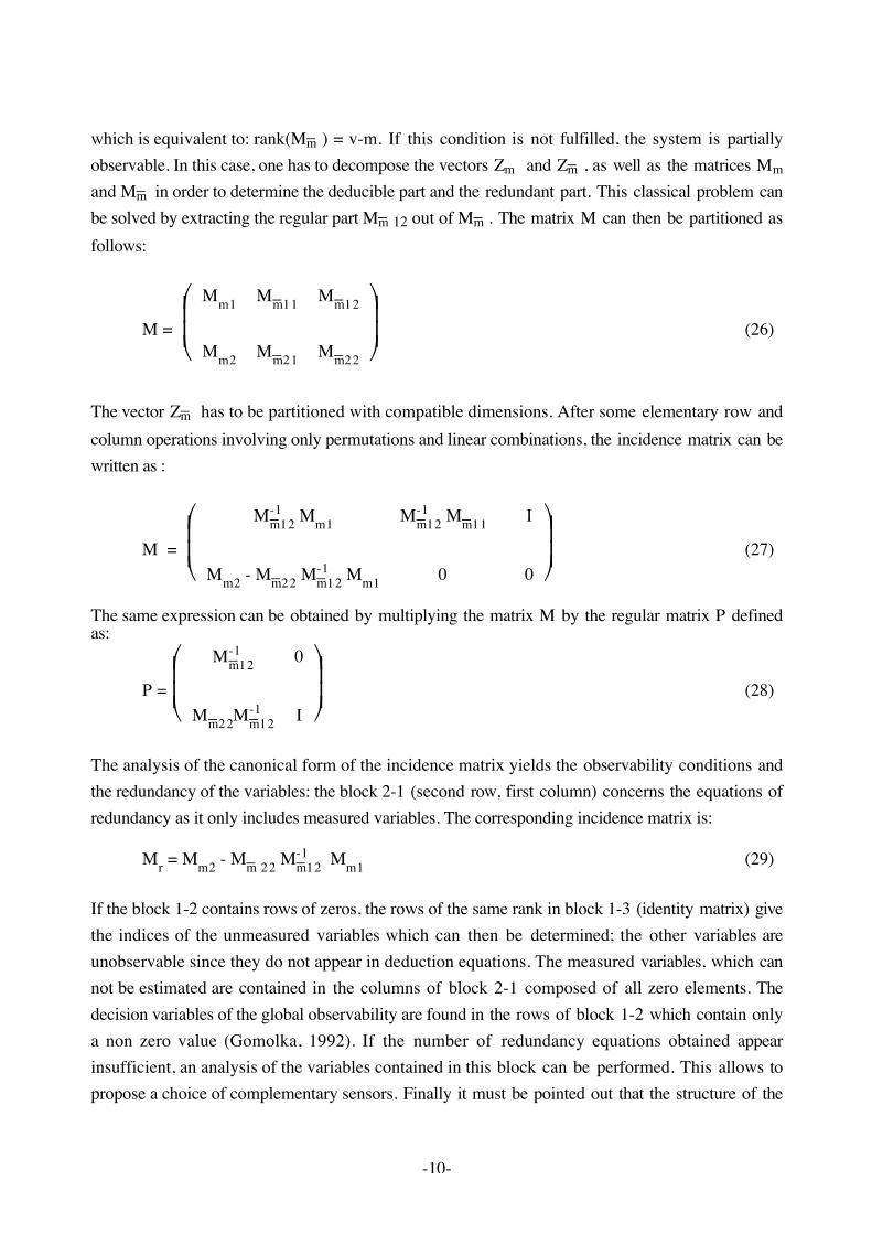
which is equivalent to: rank(Mm_ ) = v-m. If this condition is not fulfilled, the system is partially

observable. In this case, one has to decompose the vectors Zm and Zm_ , as well as the matrices Mm

and Mm_ in order to determine the deducible part and the redundant part. This classical problem can

be solved by extracting the regular part Mm_ 12 out of Mm

_ . The matrix M can then be partitioned asfollows:

M =

Mm1 Mm

_11 Mm

_12

Mm2 Mm_

21 Mm_

22

(26)

The vector Zm_

has to be partitioned with compatible dimensions. After some elementary row andcolumn operations involving only permutations and linear combinations, the incidence matrix can bewritten as :

M =

M-1

m_

12 Mm1 M-1m_

12 Mm_

11     I

Mm2 - Mm_

22 M-1m_

12 Mm1 0     0 (27)

The same expression can be obtained by multiplying the matrix M by the regular matrix P definedas:

P =

M-1

m_

12 0

Mm_

22M-1m_

12 I (28)

The analysis of the canonical form of the incidence matrix yields the observability conditions andthe redundancy of the variables: the block 2-1 (second row, first column) concerns the equations ofredundancy as it only includes measured variables. The corresponding incidence matrix is:

Mr = Mm2 - Mm_ 22 M-1

m_

12 Mm1 (29)

If the block 1-2 contains rows of zeros, the rows of the same rank in block 1-3 (identity matrix) givethe indices of the unmeasured variables which can then be determined; the other variables areunobservable since they do not appear in deduction equations. The measured variables, which cannot be estimated are contained in the columns of block 2-1 composed of all zero elements. Thedecision variables of the global observability are found in the rows of block 1-2 which contain onlya non zero value (Gomolka, 1992). If the number of redundancy equations obtained appearinsufficient, an analysis of the variables contained in this block can be performed. This allows topropose a choice of complementary sensors. Finally it must be pointed out that the structure of the

-11-

matrix Mr is not unique as it depends, in particular, on the vectors composing the regular part Mm_

12. This last point can be useful for generating structured redundancy equations i.e. equations in

which a particular group of variables appear preferentially. As described by Gertler (1990, 1991),some transformations may be used to generate these structured equations which are more sensitiveto specific faults.

This decomposition leads to a classification of the variables into the following categories: i)measured and observable variables (as these variables are bound by redundancy equations, theconsistency of the measurements can be tested by analyzing the magnitude of the equationresiduals), ii) measured and non estimable variables (these variables do not appear in a redundancyequation), iii) unmeasured and deducible variables (these variables are deduced from the variablesbelonging to the previous categories), iv) unmeasured and non estimable variables (these variablesdo not appear in the deduction equations and cannot be corrected; further measurements arenecessary to render these variables observable). This decomposition according to observability canbe generalized to the case of bi-linear (Crowe 1989, Maquin 1987) and n-linear systems (Ragot,1990b). In the second section of our paper, we will show how this decomposition can be applied tothe case of dynamic systems.

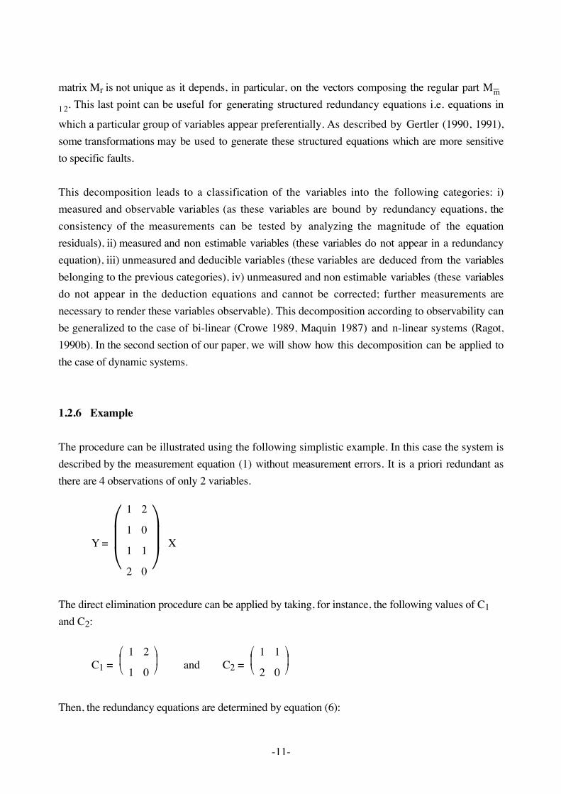
1.2.6 Example

The procedure can be illustrated using the following simplistic example. In this case the system isdescribed by the measurement equation (1) without measurement errors. It is a priori redundant asthere are 4 observations of only 2 variables.

Y =

1 2

1 0

1 1

2 0

X

The direct elimination procedure can be applied by taking, for instance, the following values of C1and C2:

C1 =

1 2

1 0 and C2 =

1 1

2 0

Then, the redundancy equations are determined by equation (6):

-12-

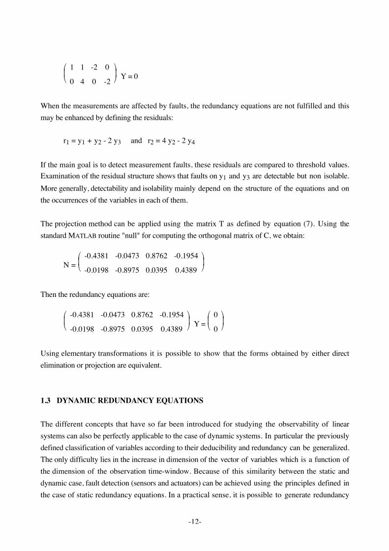
1 1 -2 0

0 4 0 -2 Y = 0

When the measurements are affected by faults, the redundancy equations are not fulfilled and thismay be enhanced by defining the residuals:

r1 = y1 + y2 - 2 y3 and r2 = 4 y2 - 2 y4

If the main goal is to detect measurement faults, these residuals are compared to threshold values.Examination of the residual structure shows that faults on y1 and y3 are detectable but non isolable.More generally, detectability and isolability mainly depend on the structure of the equations and onthe occurrences of the variables in each of them.

The projection method can be applied using the matrix T as defined by equation (7). Using thestandard MATLAB routine "null" for computing the orthogonal matrix of C, we obtain:

N =

-0.4381 -0.0473 0.8762 -0.1954

-0.0198 -0.8975 0.0395 0.4389

Then the redundancy equations are:

-0.4381 -0.0473 0.8762 -0.1954

-0.0198 -0.8975 0.0395 0.4389 Y =

0

0

Using elementary transformations it is possible to show that the forms obtained by either directelimination or projection are equivalent.

1.3 DYNAMIC REDUNDANCY EQUATIONS

The different concepts that have so far been introduced for studying the observability of linearsystems can also be perfectly applicable to the case of dynamic systems. In particular the previouslydefined classification of variables according to their deducibility and redundancy can be generalized.The only difficulty lies in the increase in dimension of the vector of variables which is a function ofthe dimension of the observation time-window. Because of this similarity between the static anddynamic case, fault detection (sensors and actuators) can be achieved using the principles defined inthe case of static redundancy equations. In a practical sense, it is possible to generate redundancy

-13-

equations from state equations under either in time or frequency domain. These two approaches aretotally equivalent (Lou, 1982) if some conditions of duration of the observation time-window arerespected. Whatever the approach, the basic principle is the same: the unknown variables areeliminated so that only known or measured variables appear in the equations.

1.3.1. Presentation

Consider the following deterministic model (equation 30) where x is the n-dimensional state vector,A is a n.n matrix, B a n.m matrix, C a p.n matrix. The vectors u and y correspond to the knowninputs and outputs of the process. In all the following treatments, without loss of generality, themeasurement y depends only on the state x and do not include the input u.

x(k+1) = A x(k) + B u(k) (30a)y(k) = C x(k) (30b)

Direct redundancy may exist among sensors whose outputs are algebraically dependent; thiscorresponds to the situation where the variable measured by one sensor can be determinedinstantaneously by other sensor measures. This direct redundancy is very useful for sensor failuredetection but is not applicable for the detection of actuator failures. In this situation, the temporalredundancy which links sensor outputs and sensor inputs must be established. When integrated on[k, k + r] window, the system (30) is expressed as:

Y(k, r) - G(r) U(k, r) = H(r) x(k) (31)

where Y is the p(r+1) vector of the outputs y(k) to y(k+r), U is the mr vector of the inputs u(k) tou(k+r), G a p(r+1).(mr) matrix and H a p(r+1).n matrix; H(r) is called the r-order observabilitymatrix of the process.

With noise on the output measurement, this equation becomes:

Y(k, r) - G(r) U(k, r) = H(r) x(k) + ε(k) (32)

1.3.2 Bases of redundancies generation

In equation (31), the input u as well as the output y of the process are known. For generatingredundancy, the unknown state vector, x(k), has to be eliminated. As equation (31) has the samestructure as equation (1), the principles described previously for generating the redundancy

-14-

equations may be directly applied to equation (31). The redundancy equations which link Y and U,independently of x, are obtained by multiplying the system (31) by the matrix Ω (called the paritymatrix) which must be orthogonal to H(r) (for simplicity the covariance matrix of the measurementerrors is taken as unity):

Ω H(r) = 0 (33)

Then, the general form of the parity equations are:

P(k) = Ω (Y(k, r) - G(r) U(k, r)) = Ω ε(k) (34)

P(k) is referred to as the generalized parity vector which is non-zero mean when a failure occurs.Under a no failure situation P(k) characterizes all the possible relationships between the inputs andthe outputs. If a measurement is biased, the parity vector is oriented along a specific direction.However, it must be pointed out that parity equations (34) are not necessarily independent,particularly if the observation window [k, k + r] is too "large". This problem can be ironed out byexpressing first the redundancy equations for each sensor (self redundancy), then the redundancyequations between different sensors (inter-redundancy) (Brunet, 1990).

1.3.3 Direct redundancy (self-redundancy)

The notion of direct redundancy (self-redundancy) is very useful for describing analyticalredundancy as it expresses the relationships between the time output of a single sensor. The jth termof the observation vector is selected; it is characterized by the submatrix Cj. Equation (31) is thenreduced to:

Yj(k, r) - Gj(r) U(k, r) = Hj(r) x(k) (35)

Hj and Gj are deduced using the definitions already given for H and G by replacing C by Cj.

In that case, the single sensor parity relation is simply defined as:

Pj(k) = Ω (Yj(k, r) - Gj(r) U(k, r)) (36)

The value of the length of the observation window, r, has not yet been specified. The parity equationswith minimal r value are particularly interesting. They can be found very simply by using the well-known Cayley-Hamilton theorem which implies that there is an rj such that:

if r < rj rank (Hj(r)) = 1 + r (37a)and if r ≥ rj rank (Hj(r)) = rj (37b)

-15-

As the row (rj + 1) of the matrix Hj(rj) is a linear combination of the rj other rows, there is a vectorΩ such that:

Ω

Cj

CjA

.

CjArj

= 0 (38)

We then obtain the redundancy equation for the jth sensor or self-redundancy:

Pj(k) = Ω (Yj(k, rj) - Gj(r) U(k, rj)) (39)

It also represents a temporal redundancy linking the actuator inputs to the temporal behavior of thejth sensor. This equation involves one sensor only. Thus, if the actuators function properly, thisrelation can be used as a self test for sensor j. However, if both actuators and sensors are defective,the occurrence of a failure can be detected, but the fault cannot be located.

As an example, let us consider the system described by the state matrices:

A =

0.7 0.2

0 0.5 B =

0

1 C =

1 0

0 1

and observed on the window [k, k + 2].

For the first sensor, C1 = (1 0) and for a window [k, k+2] the rank r1 of the observabilitymatrix H1(2) is equal to 2. The third row of the matrix H1(2) can be expressed as a linearcombination of the others. For determining this linear combination the matrix Ω is calculatedaccording to equation (33). Then the application of (39) yields the parity equation and therefore theself-redundancy of the first and the second sensors:

(0.35 - 1.2 q + q2) y1(k) = 0.2 u(k)(-1 + 2q) y2(k) - 2 u(k) = 0

where q is the shift forward operator for a discrete signal (q f(t) = f(t+1)). The two last equationsrepresent the direct temporal redundancy of the output sensors.

1.3.4 Redundancy between sensors (inter-redundancy)

-16-

Temporal redundancy exists between several sensors. For each observation matrix (built from onesingle output and all the inputs), let us retain only the rj first independent rows (rj has been definedby using the Cayley-Hamilton theorem).

Yi(k, ri-1) = Hi(ri-1) x(k) + Gi(ri-1) U(k, ri-1) i = 1, ..., p (40)

In order to obtain a formulation which is valid for all the outputs, we can introduce the commonvector U(k, r) (where r = max(r1, r2, ..., rp) of all the inputs U(k, ri-1); it may also be necessary tocomplete some matrices Gi with zero columns in order to define a common G matrix. Using trivialdefinitions system (40) can be written under a more compact form as:

Y(k, r1, ..., rp) = H(r) x(k) + G(r) U(k, r) (41)

As in the previous case, we define the matrix Ω, orthogonal to H(r). The parity equations are thenwritten as:

P(k) = Ω (Y(k, r1, ..., rp) - G(r) U(k, r)) (42)

In practice, the inter-redundancy equations are obtained by linear combinations of the self-redundancy equations. Although inter-redundancy equations are not independent of the self-redundancy equations, their particular structure make them useful for isolating failures.

Using the same example as above, we can determine the inter-redundancy equations. For the firstand the second sensor, the independent rows are:

Y1(k, 1) =

C1

C1A x(k) +

0

C1B u(k) (43a)

Y2(k, 0) = ( )C2 x(k) (43b)

By combining equations (43a) and (43b) equation (41) becomes:

Y(k, 2, 1) =

C1

C1A

C2

x(k) +

0

C1B

0

u(k)

Solving (33) gives Ω = ( 3.5 -5 1), which leads to the inter-redundancy equation:

3.5 y1(k) - 5 y1(k+1) + y2(k) = 0

-17-

Finally, the redundancy equations are:

5 y1(k+2) - 6 y1(k+1) + 1.75 y1(k) - u(k) = 0- y2(k) + 2 y2(k+1) - 2 u(k) = 03.5 y1(k) - 5 y1(k+1) + y2(k) = 0

It should be noted that the inter-redundancy equation may be obtained as a linear combination of theself-redundancy equations through the elimination of the input u. If the actuators are assumed to befully reliable, the first equation is only sensitive to the failure of the first sensor whereas the secondequation is only affected by the failure of the second sensor. Hence, these two equations can be usedto identify sensor failures only. The third equation is only affected by sensor failures even if theactuators are faulty; thus it is possible to isolate the failure of a sensor or of an actuator as theirsignatures of failure are different.

1.3.5 Direct generation of the redundancy equations

The generation of the redundancy equations can be performed in a more direct way from the stateequations of the system. This can be achieved simply by eliminating the unknown variables x so thatonly known or measured variables u and y are considered. Using the state equations (28) thefollowing relations between x, u et y can be written:

(q I - A) x(k) = B u(k) (44a)y(k) = C x(k) (44b)

Eliminating X between (44a) and (44b) gives the redundancy relation:

r(k) = y(k) - C (q I - A)-1 B u(k) = 0 (45)

Despite possible difficulties involving the calculation of the inverse of (q I - A), this formulation isquite advantageous as it directly provides redundancy relations for each output which allows toisolate the influence of each sensor. X can also be eliminated by reporting the value of X obtainedfrom equation (44b) into equation (44a). As C is not regular, the general solution of (44b) is writtenas a function of an arbitrary vector w and the generalized inverse C- of C:

x(k) = C- y(k) + (I - C-C) w(k) (46)

Equation (44a) then depends on y(k), u(k) and w(k). Redundancies are then obtained through theelimination of the arbitrary vector w(k). This can be achieved by premultiplying this equation by a

-18-

matrix Ω orthogonal to the matrix (q I - A) (I - C-C). This matrix Ω can be obtained in a simple way,taking into account the binomial character of the matrix (q I - A).

We can now examine the structure of the redundancy equations when failures of both sensors andactuators are considered. For fault detection purpose, let us assume that the effects of actuator andsensor failures can be modelled by rewriting the dynamics of the process as:

x(k+1) = A x(k) + B u(k) + Fl l(k) (47a)y(k) = C x(k) + Em m(k) (47b)

where l(k) and m(k) are some unknown time functions identically equal to zero when the actuatorsand the sensors are functioning properly. The elimination of x(k) between these equations yields theresidual equations:

r(k) = y(k) - C (q I - A)-1 B u(k) (48a)r(k) = Em m(k) + C (q I - A)-1 Fl l(k) (48b)

Equation (48a) represents the computational form of the parity equation (which contains onlyknown quantities) and equation (48b) is the internal form which contains the faults. Furthermore,using equation (48b), it is possible to explicit the conditions of isolability of sensors and actuatorsfailures according to the rank of the matrix (Em C (q I - A)-1 Fl ).

Let us return to the redundancy equation (45). The corresponding residuals can be directlycomputed by determining the resolvent matrix (q I - A)-1. However, when the order of the systembecomes high, this approach is extremely sensitive to numerical round-off errors. Differenttechniques can be used for solving this problem: decomposition of (q I - A)-1 using the algorithm ofLeverrier-Sourriau (Faddev, 1963), calculation of the transfer function relating every input to everyoutput (Bingulac 1975, Varga 1981), triangularisation of the state equations (Blackwell, 1984) and(Hashim, 1990). The algorithm proposed in Misra (1987) uses orthogonal similarity transforma-tions to find the minimal order subsystem corresponding to each input-output pair. As an alternative,the H∞ approach (Kailath 1980, Vidyasagar 1985) has been used for generating transfer functionsand redundancy equations through the double coprime factorization (Viswanadham 1987, Ding1990 and Fang 1991). Despite some numerical problems involved in the calculation of the inversematrix, the direct generation of redundancy equations is still a very powerful method as theequations obtained reveal the influence of each input and output. This is very helpful for detectingsensors and actuators failures. In particular, the influence of the outputs can be separated moreclearly by applying equation (48b) separately for each line of the measurement matrix C. Thistreatment yields a redundancy equation for each output. The same applies to the inputs if they arecarefully isolated in the following way:

-19-

x(k+1) = A x(k) + Bi ui(k) + B_

i u_ i(k) i=1, ..., r (49)

where Bi is the ith column of B and B_

i is the n(r-1) matrix obtained from B by deleting Bi. Let ui(k)

be the ith entry of u(k) and u_ i(k) the (r-1) column vector obtained from u(k) by deleting ui(k). By

premultiplying (49) by the matrix Ei (chosen orthogonal to B_

i) we obtain an equation dependingonly on a single input ui(k). The principle defined previously for eliminating the state x can still beapplied. In a more general sense, this technique affords the generation of redundancy equations inthe case of singular systems. Finally the technique of direct elimination can be applied to the case ofsystems with unknown inputs by generalizing the measurement equation (30b) considering that ydepends on x and u.

It is worth mentioning that redundancy equations can also be generated using the observer equationsassociated with the system (30). In that case the output y is compared with the output modelled bythe observer. This technique has been thoroughly explored and used for system diagnosis (Clark1978, Patton 1989a, Frank 1990). The residuals obtained directly using the state equations orindirectly using the associated observer equations are equivalent. The only difference is the presenceof a filter whose poles are those of the transfer function of the system. This equivalence wasmentioned by Frank (1990) and reexamined by Staroswiecki (1991) and Magni (1991).

Let us return to the previous example. For the first sensor, C1 = (1 0) and for the second oneC2 = (0 1). The two outputs are written as :

y1(k) = C1 (q I - A)-1 B u(k) = 1

(q - 0.7)(q - 0.5) 0.2 u(k)

y2(k) = C2 (q I - A)-1 B u(k) = 1

(q - 0.5) u(k)

The parity equations write:

5 y1(k+2) - 6 y1(k+1) + 1.75 y1(k) - u(k) = 02 y2(k+1) - y2(k) - 2 u(k) = 0

The first equation is sensitive to faults concerning the first sensor. These equations are self-redundancy equations. By eliminating u(k) between the two equations the inter-redundancy equationcan be written as:

5 y1(k+2) - 6 y1(k+1) + 1.75 y1(k) - y2(k+1) + 0.5 y2(k) = 0

-20-

which may be reduced to the minimal form:

(5 q - 3.5) y1(k) - y2(k) = 0

1.3.6 Generation of redundancies by reduction of the state equations

This is an original technique for generating redundancy equations which involves only simplenumerical calculations. Let us return to the general state equations (30). If C1 is the regular part ofthe matrix C, a simple permutation of the components of x yields the decomposition:

x1(k+1)

x2(k+1) =

A11 A12

A21 A22

x1(k)

x2(k) +

B1

B2 u(k) (50a)

y(k) = C1 x1(k) + C2 x2(k) (50b)

Using the following variable changes:

x_ 1(k) = C1 x1(k) + C2 x2(k) (51a)

x_ 2(k) = x2(k) (51b)

the state equations are rewritten:

x

_1(k+1)

x_

2(k+1) =

A

_11 A

_12

A_

21 A_

22

x

_1(k)

x_

2(k) +

B

_1

B_

2

u(k) (52a)

y(k) = x_ 1(k) (52b)

As definition of the matrices A_

ij and B_

i is trivial, it will not be further developed. The elimination of

x_ 1(k) and x

_ 2(k) between equations (52a) and (52b) gives the redundancy equation:

((z I - A_

11) - A_

12 (z I - A_

22)-1 A_

21) y(k) - (B_ 1 + A

_ 12 (z I - A

_ 22)-1 B

_ 2) u(k) = 0 (53)

Considering the size of the matrix to be inverted, this form appears to be more advantageous than(50). However, this size may still be too large. A more interesting presentation of the equation is

obtained by eliminating the variable x_ 1(k) in the state equations (52):

-21-

x_

2(k+1) = A_

22 x_ 2(k) + (A

_ 21 B

_ 2 )

y(k)

u(k) (54a)

z(k) = A_

12 x_ 2(k) (54b)

with z(k) = y(k+1) - A_

11 y(k) - B_

1 u(k) (54c)

This form shows the generalized input (y(k), u(k)) which controls the evolution of the state variable

x_ 2(k) and the modified measurement z(k). Equations (54) are then structurally similar to equations

(30); therefore, the transformation used in equations (52) can be applied to equation (54). In thisway, the unobservable variables will be progressively eliminated. The full solution of this treatmentwill now be presented; the algorithm is applied sequentially and each step is referred to as having anindex "n". At step n the state equations are written:

x(n, k+1) = A(n) x(n, k) + B(n) u(n, k) n = 0, ..., N (55a)y(n, k) = C(n) x(n, k) n = 0, ..., N (55b)

with the pseudo-measurement defined by:

y(n, k) = y(n-1, k+1) - A_

11(n-1) y(n-1, k) - B_

1(n-1) u(n-1, k) (55c)

At the final step N, different situations can appear:

First, if the matrix A reduces to a scalar matrix, the redundancy equation can be obtained without anymatrix inversion:

y(N, k) (q - A(N)) = C(N) B(N) u(N, k) (56a)

Second, if C(N) becomes null, the pseudo-measurement y(N, k) is null and the redundancy equationis generated from equation (55c) as:

y(N-1, k+1) - A_

11(N-1) y(N-1, k) - B_

1(N-1) u(N-1, k) = 0 (56b)

At each step A(n+1), B(n+1) and C(n+1) are functions of A_

ij(n) and B_

i(n) which, themselves, arefunctions of A(n), B(n) and C(n). Due to the change of variable (50), there is only one matrix to beinverted. This stage can still be avoided by applying this algorithm for all the outputs one after theother; in this case, the matrix C reduces to a row-vector and the extraction of its regular part isstraightforward.

-22-

1.3.7 Generation of redundancies by projection

After a slight rearrangement of the state equations (44), we separate the unknown variables, x, fromthe known and measured ones, u and y:

C

q I - A x(k) =

0 I

B 0

u(k)

y(k) (57)

The projection technique used in the case of static systems can also be applied to this dynamicsystem. The projection vectors α and β now become polynomials of variable q. Introducing thecombined vector ( α(q) -β(q) ) such that:

(α(q) -β(q))

C

q I - A = 0 (58)

and T the matrix such that:

C T = ( 0 I ) (59)

we know that T may be partitioned as:

T = ( )M Cr (60)

where M is a right annihilator of C and Cr a right inverse of C. A right multiplication of (58) by Tgives the equation:

β(q) (q I - A ) M = 0 (61a)α(q) - β(q) (q I - A ) Cr = 0 (61b)

This last system affords the determination of the polynomials α(q) and β(q). In particular, it mustbe noted that β(q) is orthogonal to a binomial matrix. This property facilitates its determination. Lou(1982) proposed an algorithm for a numerical determination of α and β from the nullspace of(CT (q I - A)T) by forming, in a heuristic way, a minimal base of this space. The redundancyequations can then be obtained by left multiplying equation (57) by the vector (α(q) -β(q)). Itcomes:

α(q) u(k) - β(q) B y(k) = 0 (62)

1.3.8 Generation of non independent redundancy equations

-23-

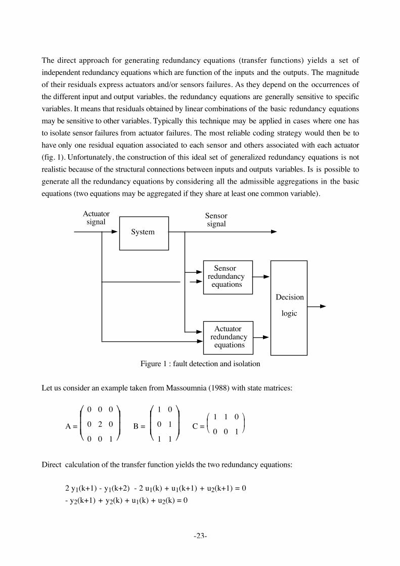
The direct approach for generating redundancy equations (transfer functions) yields a set ofindependent redundancy equations which are function of the inputs and the outputs. The magnitudeof their residuals express actuators and/or sensors failures. As they depend on the occurrences ofthe different input and output variables, the redundancy equations are generally sensitive to specificvariables. It means that residuals obtained by linear combinations of the basic redundancy equationsmay be sensitive to other variables. Typically this technique may be applied in cases where one hasto isolate sensor failures from actuator failures. The most reliable coding strategy would then be tohave only one residual equation associated to each sensor and others associated with each actuator(fig. 1). Unfortunately, the construction of this ideal set of generalized redundancy equations is notrealistic because of the structural connections between inputs and outputs variables. Is is possible togenerate all the redundancy equations by considering all the admissible aggregations in the basicequations (two equations may be aggregated if they share at least one common variable).

System

Actuator signal

Sensor signal

Sensorredundancy equations

Actuatorredundancy equations

Decision

logic

Figure 1 : fault detection and isolation

Let us consider an example taken from Massoumnia (1988) with state matrices:

A =

0 0 0

0 2 0

0 0 1 B =

1 0

0 1

1 1 C =

1 1 0

0 0 1

Direct calculation of the transfer function yields the two redundancy equations:

2 y1(k+1) - y1(k+2) - 2 u1(k) + u1(k+1) + u2(k+1) = 0- y2(k+1) + y2(k) + u1(k) + u2(k) = 0

-24-

Assuming that the actuators are fully reliable, the first equation is sensitive to the failure of the firstsensor, and the second one is sensitive to the failure of the second sensor. Hence these twoequations can be used to identify any sensor failure. By aggregation of the two equations,considering u1 or u2 as common variables, we obtain:

y1(k+2) - 2 y1(k+1) - y2(k+2) + 2 y2(k+1) + u1(k) = 0- y1(k+2) + 2 y1(k+1) + y2(k+2) - 3 y2(k+1) + 2 y2(k) + 2 u2(k) + u2(k+1) = 0

Assuming that the sensors are fully reliable, the first equation is sensitive to the failure of the firstactuator and the second equation is sensitive to the failure of the second actuator. Hence these twoequations can be used to identify any actuator failure.

It is also possible to use more general redundancy equations with a slight extension. If the basicredundancy equations are expressed in the z domain, the residual may be written:

r(k) = D(q) y(k) - N(q) u(k) = ( N(q) -D(q) )

u(q)

y(q) (63)

if we consider the generalized or structured residual:

rg(q) = J(q) (D(q) y(q) - N(q) u(q)) (64)

in which we have introduced a stable rational transfer function J(q) to add another "degree offreedom". The determination of J(q) is performed so that the new residuals rg are small undernominal conditions and large when failures are present. Therefore rg responds quickly to failuresand each different actuator and sensor failures should produce different residuals. For instance inViswanadham (1987), a unimodular matrix J is used so that J D is in upper-triangular form. Whenthe number of outputs is greater than or equal to the number of inputs, a diagonalized residual vectorcan be obtained based on a coprime factorization approach. Viswanadham shows an example of thisprocedure applied to a turbine engine control system while Gertler (1988, 1991) presents a methodfor determining the matrix J by using the concept of occurrence matrix (J is calculated so that thepositions of the null terms of the matrix J(q) ( D(q) -N(q) ) are specified). It should be noted thatthe so-called inter-redundancy and self-redundancy equations are particular cases of the structuredresiduals.

1.3.9 Interconnected systems

-25-

A linear multivariable process can be described by a set of equations:

x(k+1) = A x(k) + B u(k) (65a)y(k) = C x(k) + D u(k) (65b)

For a process composed of several sub-processes, the structure (65) is always available. However, itis very abstract and thus, meaningless to the user. The interconnections between the differentelements of the system do not explicitly appear. In order to stay closer to the physical structure ofthe process, it is preferable to use a description of each sub-system and to take into account theirconnections. In the discrete domain, the ith output Si can be expressed as a function of the ni inputsEij (j = 1, ..., ni):

Di(q) Si(k) = ∑ni

j=1 (Nij(q) Eij(k)) (66)

where Di(q) and Nij(q) are polynomials in the q variable. For all the outputs it is clear that we canuse the matricial polynomial equation:

D(q) S(k) - N(q) E(k) = 0 (67)

where D(q) and N(q) are polynomial matrices in q and E(k) and S(k) the discrete forms of thevectors of input and output variables of each linear block considered separately. Because of theinterconnections existing between the subprocesses, some components of S represent the samevariables as some components of E; the non interconnected variables belonging to E and S definethe vector X. With an evident definition for the polynomial matrix M(q), equation (67) becomes:

M(q) x(k) = 0 (68)

Some elements of the X vector are known (measurements by example); we then have a measurementequation:

y(k) = C x(k) (69)

Finally the global system can be put into the following form:

M(q)

C x(k) -

0

I y(k) =

0

0 (70)

This is a form that has been used to describe static and dynamic system. On a structural point ofview, the generation of analytical redundancy equations may be obtained, following the sameprinciple: one has to eliminate the unknown variable x in equation (70). As previously explained the

-26-

direct elimination or the projection method would be very appropriate; the only difficulty lies in thefact that the operations will have to be carried out on polynomial matrices. For applying theprojection method, one has to search a polynomial matrix T, orthogonal to the matrix P(q) = (MT(q) CT)T. It must be pointed out that the redundancy equations do not always exist (Staroswiecki 1989,1990). Indeed, if P(q) is a polynomial matrix with n rows (n = dim X + dim Y) whose rank is r, thematrix T exists iff n is greater than r. If this condition is not fulfilled, the system is not redundant.This last condition is a generalization of the condition defined in the case of static systems i.e. thenumber of variables had to be less than the number of measurement equations.

1.3.10 Observability decomposition

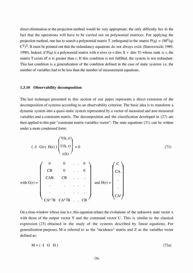
The last technique presented in this section of our paper represents a direct extension of thedecomposition of systems according to an observability criterion. The basic idea is to transform adynamic system into a quasi-static system represented by a vector of measured and non measuredvariables and a constraint matrix. The decomposition and the classification developed in (27) arethen applied to this pair "constraint matrix-variables vector". The state equations (31) can be writtenunder a more condensed form:

( -I G(r) H(r) )

Y(k, r)

U(k, r)

x(k)

= 0 (71)

with G(r) =

0 0 . . 0

CB 0 . . 0

CAB CB . . .

. . . . .

. . . . .

CAr-1B CAr-2B . . CB

and H(r) =

C

CA

.

.

CAr

On a time-window whose size is r, this equation relates the evolutions of the unknown state vector xwith those of the output vector Y and the command vector U. This is similar to the classicalexpression (23) obtained in the study of the systems described by linear equations. Forgeneralization purposes, M is referred to as the "incidence" matrix and Z as the variables vectordefined as:

M = ( -I G H ) (72a)

-27-

ZT = ( YT UT xT ) (72b)

The two first blocks in (72a) correspond to the known variables (Y and U) and the last block to thenon measured variables. This is a form similar to equation (21). By transforming M into a canonicalform (equation (27)), using a decomposition according to observability, the redundancy equations(corresponding to the parity equations) as well as the deduction equations can be obtained under anexplicit form.

Let us consider the system described by the following state equations:

A =

0.7 0.2

0 0.5 B =

0

1 C =

1 0

0 1

if it is observed on a time-window whose size is equal to 2, the incidence matrix M is written:

y1(k) y2(k) y1(k+1) y2(k+1) y1(k+2) y2(k+2) u(k) u(k+1) x1(k) x2(k) -1 . . . . . . . 1 . . -1 . . . . . . . 1 . . -1 . . . . . 0.70 0.20 . . . -1 . . 1 . . 0.50 . . . . -1 . 0.20 . 0.49 0.24 . . . . . -1 0.50 1 . 0.25

The line located above this matrix recalls the names of the different variables present in equation(71). Using the proposed decomposition procedure (equation (27)), the canonical form of thismatrix is:

y1(k) y2(k) y1(k+1) y2(k+1) y1(k+2) y2(k+2) u(k) u(k+1) x1(k) x2(k) 0.49 0.14 . 0.20 -1.00 . . . . . 0.70 0.20 -1.00 . . . . . . .. 0.50 . -1.00 . . 1.00 . . .. . . .0.50 . -1.00 . 1.00 . .-1.00 . . . . . . . 1.00 .. -1.00 . . . . . . . 1.00

where the first line still corresponds to the name of the concerned variables.

The redundancy and deduction equations are then written as:

-28-

0.49 y1(k) + 0.14 y2(k) + 0.20 y2(k+1) - y1(k+2) = 00.70 y1(k) + 0.20 y2(k) - y1(k+1) = 00.50 y1(k) - y2(k+1) - u(k) = 0- y1(k) + x1(k) = 0- y2(k) + x2(k) = 0

A simple extension of this decomposition technique deals with the analysis of system with unknowninputs. The structure of such a system can be written:

x(k+1) = A x(k) + B u(k) + E d(k) (73a)y(k) = C x(k) (73b)

It can be rewritten under its matricial expression for a time-window of size r:

( I -Gu -Gd -H )

Y(k, r)

U(k, r)

D(k, r)

x(k)

= 0 (74)

This quasi-static form shows the known and unknown parts of the variables vector and thecorresponding partitioning of the incidence matrix. The procedure of decomposition according toobservability developed in the static case can then be applied to this equation.

1.4 RESIDUALS ANALYSIS

The first two sections were devoted to the generation of redundancy equations for linear static anddynamic systems. As already mentioned, the second stage of FDI concerns the so-called residualsevaluation i.e. the forming of diagnostic decision on the basis of the residuals. To limit the length ofthe present paper, all the aspects of this stage will not be covered in this section. We will especiallyfocus on the methods issued from static systems analysis and which can be extended to dynamicsystems (Maquin, 1991b). As indicated by Gertler (1988, 1990), the decision making stage usuallyimplies statistical testing. There is a close relationship between statistical testing and residualgeneration. Residuals are variables that are zero under ideal circumstances; they become nonzero asa result of failures, noise and modelling errors. To account for the presence of noise, statisticaltesting is applied to the residuals. Then, a logical pattern is generated showing which residuals canbe considered normal and which ones indicate faults. Such a pattern is called the signature of the

-29-

failure. The final step of the procedure is the analysis of the logical patterns obtained from theresiduals. The aim is to isolate the failures. Such analysis may be performed by comparison to a setof signature known to belong to simple failures.

1.4.1 Presentation

In this section, residuals generated either from static or dynamic systems are analyzed in a unifiedframework. A linear system can be described, in the fault-free case, by the following relations:

a model equation : M X* = 0 (75a)a measurement equation : Z = H X* + ε (75b)

where X* is the v-dimensional vector of process variables, Z the m-dimensional vector ofmeasurements, M the n.v matrix of model equations (without loss of generality, it is supposed of fullrow rank), H the m.v measurement selection matrix and ε is a vector of random errors characterizedby its variance matrix.

For dynamic processes, the model, which relates the state vector x(k) to the input vector u*(k) andthe output vector y*(k), described in state space discrete form, may be written as :

x(k+1) = A x(k) + B u*(k) (76a)y*(k) = C x(k) (76b)

where u*(k) and y*(k) denote the actual values of the input and output of the system. Defining, on atime-window of length N, the mixed vector of inputs and states:

X* = ( x(0) u*(0) x(1) u*(1) ... u*(N) x(N+1) )T (77)

and the corresponding constraints matrix:

M =

A B -I . . . . .

. . A B -I . . .

. . . . . . . .

. . . . . A B -I

(78)

the constraint equation (75a) may be condensed into the form:

M X* = 0 (79a)

Similarly, the measurement equation may be written as:

-30-

Z = H X* + ε (79b)

As the inputs and only a part of the state (equation (76b)) are measured, the selection matrix H isdefined by:

H =

C . . . . .. I . . . .. . C . . .. . . I . .. . . . . .. . . . . C

(80)

As equations (79a) and (79b) are strictly identical to (75a) and (75b), static and dynamic systemscan be analyzed in a unified framework.

The methods for fault detection and isolation are often divided into two groups: those which apply apriori, without carrying out the full data reconciliation (estimation of process variables), by directlytesting the residuals issued from redundancy equations and those which apply a posteriori on theresiduals generated by calculating the differences between the raw measurements and theirestimations. In practice, both methods are used together in order to improve the robustness of theprocedure of fault detection and isolation.

The estimation or data reconciliation problem of system (75) involves finding a set of adjustmentssuch that the adjusted values verify the model equation (75a). With the classical assumption that themeasurement errors ε are normally distributed with zero mean and known variance matrix V, thisoptimization problem can be stated as maximizing the probability density function (Ragot, 1990a):

P(Z) = 1

(2π)m/2 |V|1/2 exp(- 12 (Z - H X*) T V-1 (Z - H X*)) (81)

subject to M X* = 0

The solution X̂ of this problem is obtained by minimizing the criterion:

φ = 12 (Z - H X̂) T V-1 (Z - H X̂ ) (82a)

subject to the constraint M X̂ = 0 (82b)

Assuming that the system is observable, i.e. the knowledge of the model M and the measurementvector Z is sufficient to determine a unique estimation X̂ , allows us to write the relation:

-31-

rank

H

M = dim(X*) = v (83)

This condition is equivalent to the following one:

rank(HT V-1 H + MT M) = v (84)

Using the Lagrange multipliers technique leads to the classical unbiased estimator:

X̂ = (G-1 - G-1 MT (MG-1MT)-1 M G-1) HT V-1 Z (85)

where the regular matrix G is defined by:

G = HT V-1 H + MT M (86)

These general expressions may be simplified either if all the variables are measured or if apreliminary extraction of the redundant part of the system is achieved. In this case, system (75)reduces to:

Mr Xr* = 0 (87a)Z = Xr* + ε (87b)

where Xr* denotes the actual redundant process variables. In order to simplify the further notations,we will drop, in the following, the subscript r. Estimation of the redundant variables Xr are given bythe classical result:

X̂ = (I - V MT (MVMT)-1M) Z (88)

Using the formula giving the variance of a linear combination of random variables, it can be provedthat the variance-covariance matrix of the estimated vector X̂ is expressed by:

V̂ = (I - V MT (MVMT)-1M) V (89)

The vector E of adjustments (or residuals) and the residual criterion φR are obtained by directsubstitution:

E = Z - X̂ = V MT (MVMT)-1M Z (90)

φR = ET V-1 E (91)

Both the vector of adjustments E (90) and the direct imbalances vector of redundancy equations Rdefined by :

R = M Z (92)

-32-

can be considered and processed as residuals. However, it should be noticed, that these residualscannot be analyzed in the same way as each entry of R is associated with an equation and each entryof E with a specific variable.

1.4.2 Residual criterion analysis

A first approach to testing the residuals is to introduce a single scalar statistic like, for example, theresidual criterion (91). As was first pointed out by Reilly (1963), the residual criterion:

φR = ET V-1 E (93)

has a chi-square distribution with a number of degrees of freedom equal to the rank of M.Furthermore, it is also useful to note that the calculation of φR does not require the estimation stage.It is easy to show that the residual criterion can be expressed as a function of R:

φR = RT(MVMT)-1R (94)

Thus the residuals can be globally tested against tabulated values of chi2. In the fault-free case, thefunction φR is below the threshold for the chi-square with the appropriate confidence level andnumber of degrees of freedom. Unfortunately, if the chi-square test is satisfied, it does not prove thatthere are no faults in the measurements set since a fault may exist among a large set ofmeasurements. It is then preferable to use further specific tests to diagnose the measurements.

A difficulty with this global test is that, while it indicates well the presence of fault it is not able toidentify the source of these errors. The use of a sequential procedure allows the location of the fault.Ripps (1962) proposed a scheme that was also used by Nogita (1972) under a slightly modifiedform. For the set of all process measurements, one first calculates the global test φR. If an error isindicated by the test, all measurements are considered as suspect candidates. Then, themeasurements are "deleted" sequentially from the process (in groups of size 1, 2, ...). After eachdeletion the global test is again applied. In this approach, the purpose is to assess the effect ofdeleting a particular set of measurements on the objective function and on the estimations.Furthermore, it is possible to have the same approach as the one developed in the case of multiple-observer for state reconstruction (Frank, 1989) by comparing together the different estimationsobtained after each deletion.

Romagnoli (1981) and later Fayolle (1987) consider suspect measurements by assigning them aninfinite variance. The corresponding variation of the criterion φR is then used to detect the possible

-33-

faults. By isolating the measurement z2, for which the variance will be later modified, let us considerthe following partitioning of the matrices:

M = ( M1 m2 ) (95)

Z = ( Z1 z2 ) (96)

At the same time, let us consider a modification Δv2 of the variance of this measurement. Then, thewhole variance matrix is written as:

V+ΔV =

V1 0

0 v2+Δv2 (97)

The residual criterion is then modified as:

φR+ΔφR = RT (M (V+ΔV) MT)-1 R (98)

from which, when Δv2 is infinite, the following variation can be deduced:

ΔφR = - RT K m2 m2

T K Rm2

T K m2 (99)

withK = (MVMT)-1 (100)

Equation (99) gives a simple expression of the reduction in the objective function when deleting asingle measurement. Thus, aside from vector-matrix multiplications, the only computation needed isthe calculation of K carried out once and only once whatever the suspect measurement. Crowe(1988) has also developed formulas to predict the effects of deleting any set of measurements on theobjective function. These formulas can be used without having to compute the reconciliation for eachcase of deletion.

1.4.3 Imbalances or adjustments vectors analysis

Another approach is the direct parallel testing of the residuals. With the assumption of a Gaussiandistribution of the measurement errors, the vector R also follows a normal distribution with zeromean and covariance VR:

VR = M V MT (101)

In order to compare the elements of the R vector, let us define a standardized imbalance vector RN:

-34-

RN = diag(VR)-1/2 R (102)

Each entry RN(i) follows a normal distribution with zero mean and unity variance. A simplestatistical two tailed test can therefore be used: we may conclude that equation i is a "bad" equationif:

| RN(i) | > t (103)

Classically, one may choose the critical constant t to control the familywise Type I error rate at somepre-assigned level α. Even if we assume the presence of only one gross error, the relationshipbetween the "bad" equation(s) and the suspect measurement is not straightforward. It depends onthe structure of the equations and the location of the faults. In some cases, we are not able to suspectone measurement only. For solving this case (Mah, 1976) proposed to apply the preceding test toeach equation and also to the aggregates of two or more equations (also known as pseudo-equations). The main assumption underlying this method is that faults do not cancel each other.

This latter approach can also be applied to the adjustments vector E. The variance matrix of thisvector is expressed as:

VE = V MT (MVMT)-1 M V (104)

As for the imbalance residuals vector, we define the standardized adjustments vector:

EN = diag(VE)-1/2 E (105)

Each EN(i) is compared with a critical test value. If at least one entry of EN is out of the confidenceinterval then, there is a "bad" measurement. The defective measurement can always be shown tocorrespond to the greatest standardized adjustment residual (Fayolle, 1987).

For the linear case, instead of (105), Tamhane (1985) has shown that for a non diagonal covariancematrix V, a vector of test statistics with the maximal power for detecting a single fault is obtained bypremultiplying E by V-1. Then, the transformed residual, e = V-1 E, is normally distributed with zeromean and a variance matrix Ve = V-1 VE V-1. The power of the test (the probability of correctlydetecting and identifying gross errors when they are present in the process data) has beenestablished and discussed by Iordache (1985) under different conditions (various networks, errorslocation, variance values ...) using the Monte Carlo simulation.

Note that Jongenelen (1988) pointed out the case where the variance V depends on an unknownscale factor σ2; on this basis, he proposes a new test based on externally Studentized residuals.

-35-

1.4.4 Generalized likelihood ratio approach

A new formulation of the problem of gross error detection is due to Narasimhan (1987). Thisapproach, the generalized likelihood ratio test, was first developed by Willsky and Jones (1976) toidentify abrupt failures in dynamic systems. It is based on the classical likelihood ratio test. If nofaults are present, the mathematical expectation of R (equation (92)) is null and its variance matrix isgiven by (101). If a fault of magnitude b is present in the measurement of variable i, themathematical expectation of R can be written:

E(R) = b M ei = b fi (106)

where ei is an elementary vector with 1 at the position i and zeros elsewhere. If we define µ as theexpected value of R, we can formulate the hypotheses for faults detection as:

H0 : µ = 0 (107)H1 : µ = b fi (108)

where H0 is the null hypothesis that no faults are present and H1 is the alternative hypothesis H1that a measurement bias is present. In order to test the hypothesis H1 and estimate the unknownparameters b and fi we use the likelihood ratio test statistics:

λ = supb,  fi

 

Prob(R/H1)Prob(R/H0)  (109)

Using the normal probability density function for R, we can write (109) as:

λ = supb,  fi

exp(- 

12 (R - b fi)T VR

-1 (R - b fi))

exp(- 12 RTVR

-1R) (110)

Since the log function is monotonic, we can simplify the calculation by choosing the test statistics:

T = 2 Log λ = supb,  fi

( RT VR-1 R - (R - b fi)T VR

-1 (R - b fi)) (111)

The computation proceeds in two steps. First, for any vector fi, we compute the estimate of b:

b̂ = (fTi VR

-1 fi)-1 (fTi VR

-1 R) (112)

Then, using equation (111), we obtain the corresponding value of T:

-36-

Ti = (fT

i  VR-1 R)2

(fTi  VR

-1 fi) (113)

This calculation is performed for every vector fi and the test statistics T is therefore obtained as:

T = supfi

Ti

The test statistic T is compared with a prespecified threshold. If T is greater than this threshold, thena fault has been detected and its magnitude is estimated with (112).

1.4.5 Parity space approach

In the early developments of fault diagnosis methods, the parity space approach was applied tohardware redundancy schemes (Potter 1977, Daly 1979, Hamad 1986). In the fault-free case, themeasurement equation is :

Z = H X* + ε (114)

where X* is the n-dimensional vector of redundant process variables, Z the m-dimensionalmeasurement vector and H an m.n measurement matrix. For such systems, the number m ofmeasurements is greater than the number n of variables (m > n). The noise vector ε has a variancematrix V.

Equations (75), which describe the general structure of redundancy equations of a linear staticsystem, can be transformed into the formulation (114) if we proceed to the elimination of the modelequation (Ragot, 1991a). For that purpose, let us extract from M, the regular part M1:

M = ( M1 M2 ) (115)

The vector X* may be decomposed following this partitioning:

X* =

X1

*

X2* (116)

As M1 is a regular matrix, X1* may be expressed :

X1* = - M1

-1 M2 X2* (117)

Then, the measurement equation takes a form which looks like (114):

-37-

Z = H X2* + ε (118)

with:

H =

- M-1

1  M2  I

(119)

The parity vector is related to the measurement vector Z through a projection matrix Ω of dimensionn.v (with n = v-m) :

p = Ω V-1/2 Z (120)

Parity equations show that, in the absence of fault, the magnitude of the parity vector is small(presence of measurement noise). If a failure occurs in only one of the sensors, then the parityvector grows in a fixed direction associated with the failed sensor. Furthermore, the components ofthe parity vector have the same probability distribution as the measurement errors which areindependent Gaussian of zero mean value. By definition (120), the variance-covariance matrix Vp ofthe parity vector p is an identity matrix.

As the variable c2 = pTV-1p p is the sum of squares of (v-m) normally distributed variables, it has a

chi-square probability distribution with (v-m) degrees of freedom and may be compared to thethreshold c2

1-α where c21-α is the value of chi-square at a confidence level α. Once the detection of

faults is made, they can be located. For each column Ωj of the projection matrix Ω, we compute theprojection of the parity vector. It is given by:

pj = Ωj

T p|| Ωj || j = 1, ..., v (121)

The defective sensor then corresponds to the greatest projection pj of p. Next, the suspect variable isdeleted from the system and the detection test is recalculated after this deletion. The procedure isstopped when the magnitude of the parity vector p corresponding to the remaining measurements nolonger fulfills the detection test.

It must be noted that, in the linear case, it is possible to establish the complete equivalence betweenall the preceding methods: residual criterion, imbalances or adjustments vectors analyses, generalizedlikelihood ratio or parity space approaches (Maquin, 1991a).

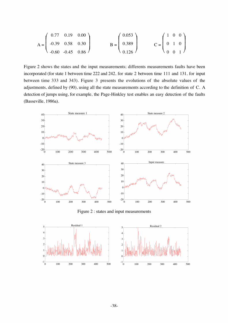
In order to illustrate one of the preceding methods, let us consider the third order dynamic systemdescribed by system (76) with the following matrices:

-38-

A =

 0.77  0.19  0.00

-0.39  0.58  0.30

-0.60 -0.45  0.86 B =

0.053

0.389

0.126 C =

1 0 0

0 1 0

0 0 1

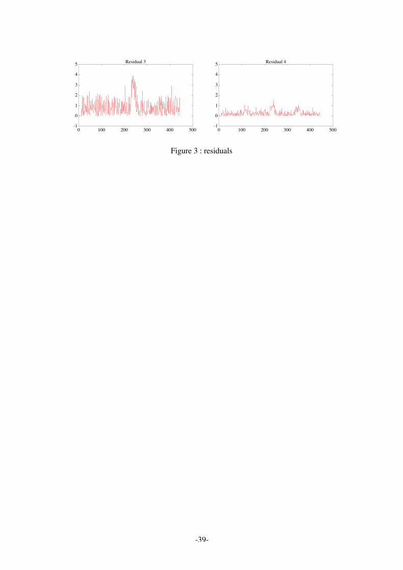
Figure 2 shows the states and the input measurements; differents measurements faults have beenincorporated (for state 1 between time 222 and 242, for state 2 between time 111 and 131, for inputbetween time 333 and 343). Figure 3 presents the evolutions of the absolute values of theadjustments, defined by (90), using all the state measurements according to the definition of C. Adetection of jumps using, for example, the Page-Hinkley test enables an easy detection of the faults(Basseville, 1986a).

-20

-10

0

10

20

30

40

0 100 200 300 400 500

State measure 1

-20

-10

0

10

20

30

40

0 100 200 300 400 500

State measure 2

-20

-10

0

10

20

30

40

0 100 200 300 400 500

State measure 3

-20

-10

0

10

20

30

40

0 100 200 300 400 500

Input measure

Figure 2 : states and input measurements

-1

0

1

2

3

4

5

0 100 200 300 400 500

Residual 1

-1

0

1

2

3

4

5

0 100 200 300 400 500

Residual 2

-39-

-1

0

1

2

3

4

5

0 100 200 300 400 500

Residual 3

-1

0

1

2

3

4

5

0 100 200 300 400 500

Residual 4

Figure 3 : residuals

-40-

REFERENCES

[ALMA 84] G.A. ALMASY, R.S.H. MAH. Estimation of measurement error variances fromprocess data. Industrial Engineering and Chemistry Process Design andDevelopment, vol. 23, p. 779-784, 1984.

[ARBE 82] A. ARBEL. Sensor placement in optimal filtering and smoothing problem. IEEETransactions on Automatic Control, vol. AC-27, n° 1, p. 94-98, 1982.

[BASS 86a] M. BASSEVILLE, A. BENVENISTE. Detection of abrupt changes in signals anddynamic systems. Lecture Notes in Control and Information Sciences, n° 77,Springer Verlag, 1986.

[BASS 86b] M. BASSEVILLE. Optimal sensor location for detecting changes in dynamicalbehavior. Rapport de Recherche n° 498, INRIA, 1986.

[BATH 82] L. BATH. Détection de défaut sur des capteurs redondants, application à une mesurede niveau d'un pressuriseur de centrale nucléaire. Mémoire CNAM, Paris, 1982.

[BING 75] S.P. BINGULAC. On the calculation of the transfer function matrix. IEEETransactions on Automatic Control, p. 134-135, 1975.

[BLAC 84] C.C. BLACKWELL. On obtaining the coefficients of the output transfer functionfrom a state space model and output model of a linear constant coefficient system.IEEE Transactions on Automatic Control, vol. AC-29, n° 12, p. 1122-1125, 1984.

[BROU 78] F. BROUSSOLLE. State estimation in power system detecting bad data through thesparse inverse matrix method. IEEE Transactions on Power Apparatus and Systems,vol. PAS-97, n° 3, p. 678-682, 1978.

[BRUN 90] J. BRUNET, M. LABARRERE, D. JAUME, A. RAULT, M. VERGE. Détection etdiagnostic de pannes. Approche par modélisation. Traité des nouvelles technologies,série diagnostic et maintenance, Hermès, 1990.

[CHOW 84] E.Y. CHOW, A.S. WILLSKY. Analytical redundancy and the design of robustfailure detection systems. IEEE Transactions on Automatic Control, vol. AC-29, n°7, p. 603-614, 1984.

-41-

[CLAR 78] R.N. CLARK. Instrument fault detection. IEEE Transactions on Aerospace andElectronic Systems, vol. AES-14, n° 3, p. 456-462, 1978.

[CLEM 90] K.A. CLEMENTS. Observability methods and optimal meter placement.International Journal of Electrical Power and Energy System, vol. 12, n° 2, p. 88-93,1990.

[CROW 83] C.M. CROWE, Y.A. GARCIA CAMPOS, A. HRYMAK. Reconciliation of processflow rates by matrix projection. Part 1 : the linear case. AIChE Journal, vol. 29, n° 6,p. 881-888, 1983.

[CROW 86] C.M. CROWE. Reconciliation of process flow rates by matrix projection. Part 2 : thenon linear case. AIChE Journal, vol. 32, n° 4, p. 616-623, 1986.

[CROW 88] C.M. CROWE. Recursive identification of gross error in linear data reconciliation.AIChE Journal, vol. 34, n° 4, p. 541-550, 1988.

[CROW 89] C.M. CROWE. Observability and redundancy of process data for steady-statereconciliation. Chemical Engineering Science, vol. 44, n° 12, p. 2909-2917, 1989.

[DALY 79] K.C. DALY, E. GAI, J.V. HARRISON. Generalized likelihood test for FDI inredundant sensor configurations. Journal of Guidance and Control, vol. 2, n° 1, p. 9-17, 1979.

[DARO 86] M. DAROUACH. Observabilité et validation des données de systèmes de grandesdimensions. Application à l'équilibrage des bilans de mesures. Thèse de doctorat-ès-sciences, Université de Nancy I, juin 1986.

[DARO 89] M. DAROUACH, J. RAGOT, M. ZASADZINSKI and G. KRAZAKALA.Maximum likelihood estimator of measurement error variances in data reconciliation.IFAC Congress AIPAC'89, Nancy 3-5 july 1989. In IFAC Symposia Series n° 5, p.109-112, Pergamon Press, 1990.

[DING 89] X. DING, P.M. FRANK. Fault detection via optimally robust detection filter.Proceedings of the 28th IEEE-CDC Conference, vol. 2, p. 1767-1782, december 13-15, Florida, USA, 1989.

-42-

[DING 90] X. DING, P.M. FRANK. Fault detection via factorization approach. Systems andControl Letters, vol. 14, p. 431-436, 1990.

[DUBU 90] B. DUBUISSON. Diagnostic et reconnaissance de formes. Traité des nouvellestechnologies, série diagnostic et maintenance, Hermès, 1990.

[FADD 63] D.K. FADDEV, D.N. FADDEEVA. Computational methods of linear algebra.Freeman, San Francisco, 1963.

[FANG 91] C.H. FANG. Determination of doubly coprime matrix fraction descriptions andcorresponding Bezout identity solutions for a regular state-space system. Systemsand Control Letters, vol. 14, p. 45-48, 1991.

[FAYO 87] J. FAYOLLE. Validation de données et diagnostic des procédés industriels. Thèse deDoctorat de l'Université de Nancy I, septembre 1987.

[FRAN 89] P.M. FRANK, J. WUNNENBERG. Robust fault diagnosis using unknown inputobservers schemes. Chapter 3, in Patton, Frank and Clark : Fault diagnosis indynamic systems, theory and application, Prentice Hall, 1989.

[FRAN 90] P.M. FRANK. Fault diagnosis in dynamical system using analytical and knowledgebased redundancy - a survey and some new results. Automatica, vol. 26, n° 3, p. 459-474, 1990.

[FRAN 91] P.M. FRANK. Fault diagnosis in dynamic systems using software redundancy.Conference on high technology information science and computer technology, Chiba,Japan, 1991.

[GERT 85] J. GERTLER, D. SINGER. Augmented models for statistical fault isolation incomplex dynamic systems. Proceedings of IEEE American Control Conference, p.317-322, Boston, MA, 1985.

[GERT 88] J. GERTLER. Survey of model based failure detection and isolation in complexplants. IEEE Control Systems Magazine, vol. 8, n° 6, p. 3-11, 1988.

[GERT 90] J. GERTLER, S. SINGER. A new structural framework for parity equation-basedfailure detection and isolation. Automatica, vol. 26, n° 2, p. 381-388, 1990.

-43-

[GERT 91] J. GERTLER. Analytical redundancy methods in fault detection and isolation.Proceedings of IFAC Safeprocess '91, vol. 1, p. 9-21, Baden-Baden, Germany, 1991.

[GOLU 83] G.H. GOLUB, G.A. MEURANT. Résolution numérique des grands systèmes.Collection de la direction des études et recherche d'EDF, Eyrolles, 1983.

[GOMO 92] W. GOMOLKA, H.C. TURBATTE, D. MAQUIN, J. RAGOT. Contribution àl'analyse de l'observabilité des systèmes linéaires. Revue RAIRO Automatique,Productique et Informatique Industrielle, vol. 26, n° 2, 1992.

[HAMA 86] M. HAMAD. Validation des mesures et détection des capteurs défaillants dans unsystème de contrôle commande. Thèse de doctorat de l'Université des sciences ettechniques de Lille Flandres Artois, juin 1986.

[HASH 90] G. HASHIM. Contribution à la réalisation et à la simplification des systèmesmultivariables. Thèse de doctorat de l'Université de Nancy I, avril 1990.

[HERA 91] N. HERAUD, D. MAQUIN, J. RAGOT. Multilinear balance equilibration.Application to a complex metallurgical process. Minerals and metallurgicalprocessing, p. 197-204, November 1991.

[HIMM 78] D.M. HIMMELBLAU. Fault detection and diagnosis in chemical andpetrochemical processes. Chemical Engineering Monograph, Elsevier, 1978.

[ISER 84] R. ISERMAN. Process fault detection based on modelling and estimation methods -a survey. Automatica, vol. 20, n° 4, p. 387-404, 1984.

[JONG 88] E.M. JONGENELEN, C.D. HEVER, G.A. VAN ZEE. Detection of gross errors inprocess data using studentized residuals. Computer Chemical Engineering, vol. 12,n° 8, p. 845-847, 1988.

[KAIL 80] T. KAILATH. Linear systems. Prentice Hall, Englewood Cliffs, N.Y., 1980.

[KELL 91] J.Y. KELLER. Contribution à la validation de données de systèmes statiques etdynamiques. Thèse de doctorat de l'Université de Nancy I, septembre 1991.

-44-

[KRAT 91] F. KRATZ. Utilisation des techniques de redondances matérielles et analytiques à ladétection de pannes de capteurs. Application aux centrales nucléaires. Thèse dedoctorat de l'Université de Nancy I, juin 1991.

[KRET 88] A. KRETSOVALIS, R.S.H. MAH. Observability and redundancy classification ingeneralized process networks, 1 : theorems. Computers and Chemical Engineering,vol. 12, n° 7, p. 671-687, 1988.

[KRUM 80] G.R. KRUMPHOLZ, K.A. CLEMENTS, S.W. DAVIS. Power system observability: a practical algorithm using network topology. IEEE Transactions on PowerApparatus and Systems, vol. PAS-99, p. 1534-1542, 1980.

[LOU 82] X.C. LOU. A system failure detection method - the failure projection method. Masterof science, MIT, June 1982.

[MAGN 91] J.F. MAGNI, Ph. MOUYON. A generalized approach to observers for faultdiagnosis. Proceedings of the 30th IEEE CDC, vol. 3, p. 2236-2241, Brighton,England, 1991.

[MAH 76] R.S.H. MAH, G.M. STANLEY, D.M. DOWNING. Reconciliation and rectificationof process flow and inventory data. Industrial Engineering Chemistry ProcessDesign Development, vol. 15, n° 1, p. 175-183, 1976.

[MAQU 86] D. MAQUIN, J. FAYOLLE, M. DAROUACH, J. RAGOT. Localization of sensorsin large scale industrial systems. Proceedings of IMACS congress, Villeneuved'Ascq, 1986. Published in Applied Modelling and Simulation of TechnologicalSystems, p. 33-39, Elsevier, 1987.

[MAQU 87] D. MAQUIN. Observabilité, diagnostic et validation de données de procédésindustriels. Thèse de doctorat de l'Université de Nancy I, novembre 1987.

[MAQU 89] D. MAQUIN, J. RAGOT, M. DAROUACH. Observability and data validation ofbilinear systems. IFAC Congress AIPAC'89, Nancy 3-5 july 1989. In IFACSymposia Series n° 5, p. 113-118, Pergamon Press, 1990.

[MAQU 91a] D. MAQUIN, J. RAGOT. Comparison of gross errors detection methods in processdata. Proceedings of the 30th IEEE-CDC, Brighton, England, December 1991.

-45-

[MAQU 91b] D. MAQUIN, G. BLOCH, J. RAGOT. Data reconciliation of measurements. Revuediagnostic et sureté de fonctionnement, vol. 1, n° 2, p. 145-181, 1991.

[MASS 88] M.A. MASSOUMNIA, W.E. VAN DER VELDE. Generating parity relations fordetecting and identifying control system component failures. Journal of Guidance,vol. 11, n° 1, p. 60-65, 1988.

[MISR 87] P. MISRA, R.V. PATEL. Computation of transfer function matrices of linearmultivariable systems. Automatica, vol. 23, n° 5, p. 635-640, 1987.

[NARA 87] S. NARASIMHAN, R.S.H. MAH. Generalized likelihood ratio method for grosserror identification. AIChE Journal, vol. 33, n° 9, p. 1514-1521, 1987.

[NARA 89] S. NARASIMHAN, R.S.H. MAH. Treatment of general steady state process modelsin gross error identification. Computers and Chemical Engineering, vol. 13, n° 7, p.851-853, 1989.

[NOGI 72] S. NOGITA. Statistical test and adjustment of process data. Industrial EngineeringChemistry Process Design Development, vol. 11, n° 2, p. 197-200, 1972.

[PAU 81] L. PAU. Failure diagnosis and performance monitoring. Marcel Dekker Ed., 1981.

[PATT 89a] R.J. PATTON, R.N. KANGETHE. Sensor fault detection on dynamic systems usingshort robust observers. IFAC Congress AIPAC'89, Nancy 3-5 july 1989. In IFACSymposia Series n° 5, p. 57-62, Pergamon Press, 1990.

[PATT 89b] R.J. PATTON, P.M. FRANK, R.N. CLARK. Fault diagnosis in dynamic systems :theory and application. Prentice Hall, 1989.

[PATT 91] R.J. PATTON, J. CHEN. A review of parity space approaches to fault diagnosis.Proceedings of IFAC Safeprocess '91, vol. 1, p. 239-255, Baden-Baden, Germany,1991.

[POTT 77] J.E. POTTER, M.C. SUMAN. Thresholdless redundancy management with arraysof skewed instruments. Integrity in Electronic Flight Control Systems, Agardograph-224, p. 1511-1525, 1977.

-46-

[RAGO 90a] J. RAGOT, M. DAROUACH, D. MAQUIN, G. BLOCH. Validation de données etdiagnostic. Traité des nouvelles technologies, série diagnostic et maintenance,Hermès, 1990.

[RAGO 91a] J. RAGOT, A. AITOUCHE, F. KRATZ, D. MAQUIN. Detection and location ofgross errors in measurements and analytical redundancies using parity spacetechnique. International Journal of Mineral Processing, vol. 31, n° 3-4, p. 281-299,1991.

[RAGO 91b] J. RAGOT, D. MAQUIN, G. BLOCH. Data reconciliation for process flow.Proceedings of the First European Control Conference, p. 1430-1435, Grenoble,France, 1991

[RAGO 92] J. RAGOT, D. MAQUIN, D. SAUTER. Data validation using orthogonal filters. IEEproceedings D, vol. 139, n° 1, p. 47-52, 1992.

[RAY 91] A. RAY, R. LUCK. An introduction to sensor signal validation in redundantmeasurement systems. IEEE Control Magazine, vol. 11, n° 2, p. 44-49, 1991.

[REIL 63] P.M. REILLY, R.E. CARPANI. Application of statistical theory of adjustment tomaterial balances. 13th Canadian Chemical Engineering Conference, Montréal,October 1963.

[RIPP 62] D.L. RIPPS. Adjustment of experimental data. Chemical Engineering Progress, vol.61, n° 55, p. 8-13, 1962.

[ROMA 81] J.A. ROMAGNOLI, G. STEPHANOPOULOS. Rectification of process measure-ment in the presence of gross errors. Chemical Engineering Science, vol. 35, n° 5, p.1849-1863, 1981.

[SCHW 70] F.C. SCHWEPPE, J. WILDES. Power system state estimation, part 1 : exact model.IEEE Transactions on Power Apparatus and Systems, vol. PAS-89, n° 1, 1970.

[SOOD 79] M.K. SOOD, G.W. REKLAITIS, J.M. WOODS. Solution of material balances forflowsheets modeled with elementary modules : the unconstrained case. AIChEJournal, vol. 25, n° 2, p. 209-219, 1979.

-47-

[STAR 89] M. STAROSWIECKI, P. DECLERK. Analytical redundancy in non linearinterconnected systems by means of structural analysis. IFAC Congress AIPAC'89,Nancy 3-5 july 1989. In IFAC Symposia Series n° 5, p. 51-56, Pergamon Press,1990.

[STAR 90] M. STAROSWIECKI, V. COCQUEMPOT, J. Ph. CASSAR. Generation ofanalytical redundancy relations in a linear interconnected systems. Proceedings of theIMACS Annals on Computing and Applied Mathematics MIM-S2 '90, Brussels,1990.

[STAR 91] M. STAROSWIECKI, V. COCQUEMPOT, J. Ph. CASSAR. Observer based andparity space approaches for failure detection and identification. Proceedings ofIMACS symposium on Modelling and Control of Technological Systems, vol. 2, p.536-541, Lille, France, 1991.

[TAMH 85] A.C. TAMHANE, R.S.H. MAH. Data reconciliation and gross error detection inchemical process network. Technometrics, vol. 27, n° 4, p. 409-422, 1985.

[TURB 91] H.C. TURBATTE, D. MAQUIN, B. CORDIER, C.T. HUYN. Analyticalredundancy and reliability of measurement system. Proceedings of IFACSafeprocess '91, vol. 1, p. 49-54, Baden-Baden, Germany, 1991.

[UENG 90] B.S. UENG, D. CHIU, W.H. CHENG. Failure detection and isolation by model costanalysis, International Journal of Systems Science, vol. 21, n° 11, p. 2247-2262,1990.

[VACL 69] V. VACLAVEK. Studies on system engineering III. Optimal choice of the balancemeasurement in complicated chemical systems. Chemical Engineering Science, vol.24, p. 947-955, 1969.

[VARG 81] A. VARGA, V. SIMA. Numerically stable algorithm for transfer function matrixevaluation. International Journal of Control, vol. 33, p. 1123-1133, 1981.

[VIDY 85] VIDYASAGAR. Control system synthesis : a factorization approach. MIT Press,Cambridge, MA, 1985.

-48-

[VISW 87] N. VISWANADHAM, J.H. TAYLOR, E.C. LUCE. A frequency-domain approachto failure detection and isolation with application to GE-21 turbine engine controlsystems. Control Theory and Advanced Technology, vol. 3, n° 1, p. 45-72, 1987.

[WATA 82] K. WATANABE, D.M. HIMMELBLAU. Instrument fault detection in systems withuncertainties. International Journal of Systems Science, vol. 13, p. 137-158, 1982.

[WILL 76] A. S. WILLSKY. A survey of design methods for failure detection in dynamicsystems. Automatica, vol. 12, n° 6, p. 601-611, 1976.

[WILL 76] A. S. WILLSKY, H.L. JONES. A generalized likelihood ratio approach to detectionand estimation of jumps in linear systems. IEEE Transactions on Automatic Control,vol. AC-21, n° 1, p. 108-112, 1976.

[WUNN 87] J. WUNNENBERG, P.M. FRANK. Sensor fault detection via robust observers.System fault diagnostics, reliability and related knowledge based approaches. Eds.Tzafestas, Singh and Schmidt, Reidel Press, p. 147-160, 1987.

[ZASA 90] M. ZASADZINSKI. Contribution à l'estimation de l'état des systèmes singuliers.Application à la validation de données des systèmes dynamiques linéaires. Thèse dedoctorat de l'Université de Nancy I, octobre 1990.