module 08 observability and state estimator design...

Intro to Observability Quantifying Observability Observability Properties Controllers & Observers Design Observer-Based Control

Module 08Observability and State Estimator Design of

Dynamical LTI Systems

Ahmad F. Taha

EE 5143: Linear Systems and ControlEmail: [email protected]

Webpage: http://engineering.utsa.edu/ataha

November 7, 2017

©Ahmad F. Taha Module 08 — Observability and State Estimator Design of Dynamical LTI Systems 1 / 24

http://engineering.utsa.edu/ataha


Introduction to ObservabilityObservability: The ability to observer what’s happening inside yoursystem (i.e., to know system states x(t))Observability: In order to see what is going on inside the systemunder observation (i.e., output y(t)), the system must beobservable. Observation: output y(t)Given this dynamical system:

x(k + 1) = Ax(k) + Bu(k), x(0) = x0,

y(k) = Cx(k) + Du(k),or x(t) = Ax(t) + Bu(t), x(0) = x0,

y(t) = Cx(t) + Du(t)a natural question arises: can we learn anything about x(t) giveny(t) and u(t) for a specific time t?Clearly, if we know x(0) and u(t) for all t, we can determine x(t) via

x(t) = eA(t−t0)x(t0) +∫ t

t0

eA(t−τ)Bu(τ)dτ

However, if x(0) if unknown, can you obtain x(t) via only y(t), u(t)?©Ahmad F. Taha Module 08 — Observability and State Estimator Design of Dynamical LTI Systems 2 / 24


Observability — 1

DTLTI system (n states, m inputs, p outputs):

x(k + 1) = Ax(k) + Bu(k), x(0) = x0, (1)y(k) = Cx(k) + Du(k), (2)

Application: given that A,B,C ,D, and u(k), y(k) are known∀k = 0 : 1 : k − 1, can we determine x(0)?

Solution:y(0)y(1)

...y(k − 1)

=

CCA

...CAk−1

x(0)+

D 0 . . . 0

CB D. . .

......

. . . . . . 0CAk−2B . . . CB 0

u(0)u(1)

...u(k − 1)



Observability — 2

y(0)y(1)

...y(k − 1)

=

CCA

...CAk−1

x(0) +

D 0 . . . 0

CB D. . .

......

. . . . . . 0CAk−2B . . . CB 0

u(0)u(1)

...u(k − 1)

Y (k − 1) = Okx(0) + TkU(k − 1) =⇒ Okx(0) = Y (k − 1)−TkU(k − 1)

Since Ok , Tk ,Y (k − 1),U(k − 1) are all known quantities, then wecan find a unique x(0) iff Ok is full rank

Observability DefinitionDTLTI system is observable at time k if the initial state x(0) can beuniquely determined from any given

u(0), . . . , u(k − 1), y(0), . . . , y(k − 1).



Quantifying Observability

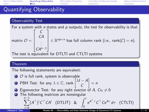
Observability TestFor a system with n states and p outputs, the test for observability is that

matrix O =

CCA

...CAn−1

∈ Rnp×n has full column rank (i.e., rank(C) = n).

The test is equivalent for DTLTI and CTLTI systems

TheoremThe following statements are equivalent:

1 O is full rank, system is observable2 PBH Test: for any λ ∈ C, rank

[λI − A

C

]= n

3 Eigenvector Test: for any right evector of A, Cvi 6= 04 The following matrices are nonsingular

n−1∑i=0

(A>)iC>CAi (DTLIT) &∫ t

0eA>τ C>CeAτ dτ (CTLTI)



Example 1

Consider a dynamical system defined by:

A =

1 −1 01 −1 00 0 0

,B =

1 00 00 1

,C =[

0 1 00 0 1

]

Is this system controllable?

Is this system observable?

Answers: Yes, Yes!

MATLAB commands: ctrb, obsv



Example 2

Determine whether the following system is observable or not:

x(k + 1) =

−1 1 0 0 0 0 00 −1 0 0 0 0 00 0 −1 0 0 0 00 0 −1 −1 0 0 00 0 0 0 0 0 00 0 0 0 1 0 00 0 0 0 0 1 0

x(k) +

01−11102

u(k)

y(k) =[

1 0 2 0 0 0 00 0 0 2 3 0 0

]x(k).

The challenge here is to be able to figure out which test should be used.Clearly, A has 7 evalues as follows: λA = {−1,−1,−1,−1, 0, 0, 0}. Test2 is the easiest test to use here. Applying the test, you’ll see that thePBH test fails for the zero eigenvalue, which means that the system isnot observable.



Unobservable SubspaceUnobservable subspace: null-space of Ok = N (Ok)It is basically the space (i.e., set of states x ∈ X that you cannotestimate or observerNotice that if x(0) ∈ Null(Ok), and u(k) = 0, then the output isgoing to zero from [0, k − 1]Notice that input u(k) does not impact the ability to determine x(0)The unobservable subspace N (Ok) is A-invariant: if z ∈ N (Ok),then Az ∈ N (Ok)

Unobservable SpaceThe null spaces Null(Ok) = N (Ok) satisfy

N (O0) ⊇ N (O1) ⊇ · · · ⊇ N (On) = N (On+1) = · · ·

This means that the more output measurements you have, the smallerthe unobservable subspace.It also implies that you cannot get more information if you go abovek > n. You can prove this by C-H theorem (An =

∑n−1i=0 αiAi )



Detectability

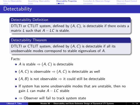
Detectability DefinitionDTLTI or CTLIT system, defined by (A,C), is detectable if there exists amatrix L such that A− LC is stable.

Detectability TheoremDTLTI or CTLIT system, defined by (A,C) is detectable if all itsunobservable modes correspond to stable eigenvalues of A.

Facts:A is stable ⇒ (A,C) is detectable

(A,C) is observable ⇒ (A,C) is detectable as well

(A,B) is not observable ⇒ it could still be detectable

If system has some unobservable modes that are unstable, then nogain L can make A− LC stable

⇒ Observer will fail to track system state©Ahmad F. Taha Module 08 — Observability and State Estimator Design of Dynamical LTI Systems 9 / 24


Observability for CT SystemsThe previous derivation for observability was for DT LTI systemsWhat if we have a CT LTI system? Do we obtain the sameobservability testing conditions?Yes, we do!First, note that the control input u(t) plays no role in observability,just like how the output y(t) plays no role in controllabilityTo see that, consider the following system with n states, p outputs,where (again) we want to obtain x(t0) (unknown):

x(t) = Ax(t), y(t) = Cx(t) x(t0) = x0 =⇒

y(t0) = Cx(t0)y(t0) = Cx(t0) = CAx(t0)y(t0) = Cx(t0) = CA2x(t0)

...y (n−1)(t0) = Cx (n−1)(t0) = CAn−1x(t0)



Observability for CT LTI Systems — 2We can write the previous equation as:

y(t0)y(t0)y(t0)

...y (n−1)(t0)

Y (t0) =

CCA

...CAn−1

︸︷︷︸=O∈Rnp×n

x(t0)⇒

x(t0) = O†Y (t0) = (O>O)−1OY (t0)Hence, the initial conditions can be determined if the observabilitymatrix is full column rankThis condition is identical to the DT case where we also wanted toobtain x(k = 0) from a set of output measurementsThe difference here is that we had to obtain derivatives of theoutput at t0Can you rederive the equations if u(t) 6= 0? It won’t make animpact on whether a solution exists, but it’ll change x(t0)



Controllability-Observability Duality, Minimality

Duality

The CT LTI system with state-space matrices (A, B, C , D) is called thedual of another CT LTI system with state-space matrices (A,B,C ,D) if

A = A>, B = C>, C = B>, D = D>.

Controllability-Observability DualityCT system (A,B,C ,D) is observable (controllable) if and only if its dualsystem (A, B, C , D) is controllable (observable).

MinimalityA system (A,B,C ,D) is called minimal if and only if it is bothcontrollable and observable.



Observer Design

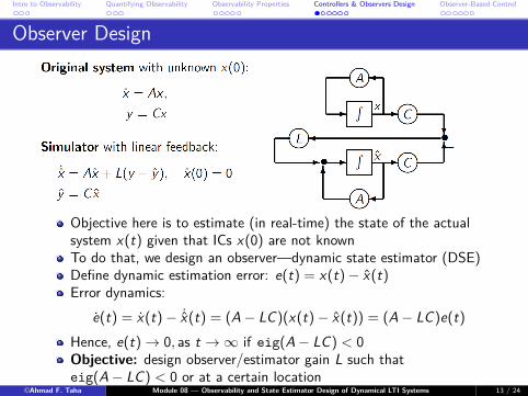
Objective here is to estimate (in real-time) the state of the actualsystem x(t) given that ICs x(0) are not knownTo do that, we design an observer—dynamic state estimator (DSE)Define dynamic estimation error: e(t) = x(t)− x(t)Error dynamics:

e(t) = x(t)− ˙x(t) = (A− LC)(x(t)− x(t)) = (A− LC)e(t)Hence, e(t)→ 0, as t →∞ if eig(A− LC) < 0Objective: design observer/estimator gain L such thateig(A− LC) < 0 or at a certain location



Example — Controller Design

Given a system characterized by A =[

1 33 1

],B =

[10

]Is the system stable? What are the eigenvalues?

Solution: unstable, eig(A) = 4,−2

Find linear state-feedback gain K (i.e., u = −Kx), such that thepoles of the closed-loop controlled system are −3 and −5

Characteristic polynomial: λ2 + (k1 − 2)λ+ (3k2 − k1 − 8) = 0

Solution: u = −Kx = −[10 11][x1x2

]= −10x1 − 11x2

MATLAB command: K = place(A,B,eig desired)

What if A =[

1 00 1

],B =

[11

], can we stabilize the system?



Example — Observer Design

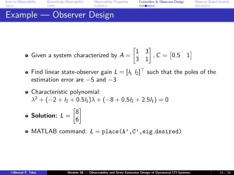
Given a system characterized by A =[

1 33 1

],C =

[0.5 1

]Find linear state-observer gain L = [l1 l2]> such that the poles of theestimation error are −5 and −3

Characteristic polynomial:λ2 + (−2 + l2 + 0.5l1)λ+ (−8 + 0.5l2 + 2.5l1) = 0

Solution: L =[

86

]MATLAB command: L = place(A’,C’,eig desired)



Observer, Controller Design for DT Systems—SummaryFor CT system

x(t) = Ax(t) + Bu(t), y(t) = Cx(t) + Du(t)– To design a stabilizing controller, find K such that

eig(Acl ) = eig(A− BK ) < 0or at a prescribed location

– To design a converging estimator (observer), find L such thateig(Acl ) = eig(A− LC) < 0

or at a prescribed locationWhat if the system is DT?

x(k + 1) = Ax(k) + Bu(k), y(k) = Cx(k) + Du(k)– To design a stabilizing controller, find K such that

−1 < eig(Acl ) = eig(A− BK ) < 1 or at a prescribed location– To design a converging estimator (observer), find L such that

−1 < eig(Acl ) = eig(A− LC) < 1 or at a prescribed location©Ahmad F. Taha Module 08 — Observability and State Estimator Design of Dynamical LTI Systems 16 / 24


Observer Design

What if the system dynamics are:

x(t) = Ax(t) + Bu(t), y(t) = Cx(t) + Du(t)

The observer dynamics will then be:

˙x(t) = Ax(t) + Bu(t) + L(y(t)− y(t))

Hence, the control input shouldn’t impact the estimation errorWhy? Because the input u(t) is know!Estimation error:

e(t) = x(t)− x(t) =⇒ e(t) = x(t) = ˙x(t) = (A− LC)(x(t)− x(t))

=⇒ e(t) = (A− LC)e(t)



MATLAB Example

Time (seeconds)0 1 2 3 4 5 6 7 8 9 10

x1,x1

-20

-15

-10

-5

0

5

10

15

x1

x1

Time (seeconds)0 1 2 3 4 5 6 7 8 9 10

x2,x2

-25

-20

-15

-10

-5

0

5

10

15

x2

x2

A=[1 -0.8; 1 0];B=[0.5; 0];C=[1 -1];% Selecting desired poleseig_desired=[.5 .7];L=place(A’,C’,eig_desired)’;% Initial statex=[-10;10];% Initial estimatexhat=[0;0];% Dynamic SimulationXX=x;XXhat=xhat;T=10;% Constant Input SignalUU=.1*ones(1,T);for k=0:T-1,u=UU(k+1);y=C*x;yhat=C*xhat;x=A*x+B*u;xhat=A*xhat+B*u+L*(y-yhat);XX=[XX,x];XXhat=[XXhat,xhat];end% Plotting Resultssubplot(2,1,1)plot(0:T,[XX(1,:);XXhat(1,:)]);subplot(2,1,2)plot(0:T,[XX(2,:);XXhat(2,:)]);



Observer-Based Control — 1

Recall that for LSF control: u(t) = −Kx(t)

What if x(t) is not available, i.e., it can only be estimated?

Solution: get x by designing L

Apply LSF control using x with a LSF matrix K to both the originalsystem and estimator

Question: how to design K and L simultaneously? Poles of theclosed-loop system?

This is called an observer-based controller (OBC)

Design questions: how shall we design K and L? Are these designsindependent?



Observer-Based Control — 2

Notice that u(t) = −Kx(t)



Observer-Based Control — 3Closed-loop dynamics:

x(t) = Ax(t)− BKx(t)˙x(t) = Ax(t) + L(y(t)− y(t))− BKx(t)

The overall system (observer + controller) can be written as follows:[x(t)˙x(t)

]=[

A −BKLC A− LC − BK

] [x(t)x(t)

]Transformation:

[x(t)e(t)

]=[

x(t)x(t)− x(t)

]=[I 0I −I

] [x(t)x(t)

]Hence, we can write:[

x(t)e(t)

]=[A− BK BK

0 A− LC

]︸︷︷︸

Acl

[x(t)e(t)

]

If the system is controllable & observable ⇒ eig(Acl) can bearbitrarily assigned by proper K and LWhat if the system isstabilizable and detectable?



Separation Principle

[x(t)e(t)

]=[A− BK BK

0 A− LC

]︸︷︷︸

Acl

[x(t)e(t)

]≡

[x(t)˙x(t)

]=[

A −BKLC A− LC − BK

] [x(t)x(t)

]

Notice the above dynamics for the OBC are equivalentWhat are the evalues of the closed loop system above?Since Acl is block diagonal, the evalues of Acl are

eig(A− BK )⋃

eig(A− LC)

eig(A− BK ) characterizes the state control dynamicseig(A− BK ) characterizes the state estimation dynamicsIf the system is obsv. AND cont. =⇒ evalues(Acl ) can be arbitrarilyassigned by properly designing K and LIf the system is detect. AND stab. =⇒ evalues(Acl ) can bestabilized via properly designing K and L



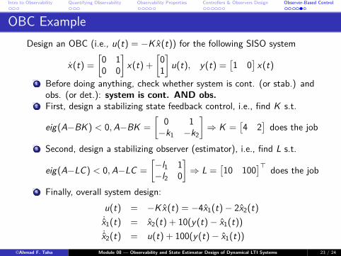
OBC ExampleDesign an OBC (i.e., u(t) = −Kx(t)) for the following SISO system

x(t) =[

0 10 0

]x(t) +

[01

]u(t), y(t) =

[1 0

]x(t)

1 Before doing anything, check whether system is cont. (or stab.) andobs. (or det.): system is cont. AND obs.

2 First, design a stabilizing state feedback control, i.e., find K s.t.

eig(A−BK ) < 0,A−BK =[

0 1−k1 −k2

]⇒ K =

[4 2

]does the job

3 Second, design a stabilizing observer (estimator), i.e., find L s.t.

eig(A−LC) < 0,A−LC =[−l1 1−l2 0

]⇒ L =

[10 100

]> does the job

4 Finally, overall system design:u(t) = −Kx(t) = −4x1(t)− 2x2(t)˙x1(t) = x2(t) + 10(y(t)− x1(t))˙x2(t) = u(t) + 100(y(t)− x1(t))



Questions And Suggestions?

Thank You!Please visit

engineering.utsa.edu/atahaIFF you want to know more ,


engineering.utsa.edu/ataha

module 08 observability and state estimator design...

Documents