modern contral systems1 lecture 06 analysis (ii) controllability and observability 6.1...

Modern Contral Systems 1

Lecture 06 Analysis (II) Controllability and Observability

6.1 Controllability and Observability

6.2 Kalman Canonical Decomposition

6.3 Pole-zero Cancellation in Transfer Function

6.4 Minimum Realization


Motivation1

2

1

2

1

2

1

01

)(0

1

10

12

x

xy

tux

x

x

x

1s 1s 1

1 2

u y1x2x

s

x )0(2

s

x )0(1

1 1x2x

1controllable

uncontrollable


DuCxy

RxBuAxx n

,

Controllability and Observability

Plant:

Definition of Controllability

A system is said to be (state) controllable at time , if there exists a finite such for any and any , there exist an input that will transfer the state to the state at time , otherwise the system is said to be uncontrollable at time .

0t01 tt )( 0tx 1x

][ 1,0 ttu )( 0tx

1x 1t

0t


1

1

)(sU

)(sY1

-1s

3 -1s 2

Example: An Uncontrollable System

xy

uxx

21

0

1

30

01

1x

2x

※ State is uncontrollable.2x

BABAABBU

nUrankBAn 12

,)(leControllab ,

0)det( U

Controllability Matrix

BABAABBU n 12Matrix ility Controllab

Ru if


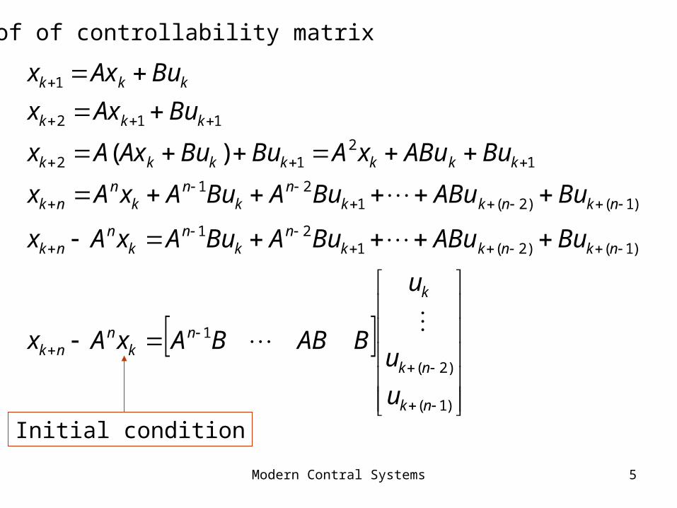
Proof of controllability matrix

)1(

)2(

1

)1()2(121

)1()2(121

12

12

112

1

)(

nk

nk

k

nk

nnk

nknkkn

kn

kn

nk

nknkkn

kn

kn

nk

kkkkkkk

kkk

kkk

u

u

u

BABBAxAx

BuABuBuABuAxAx

BuABuBuABuAxAx

BuABuxABuBuAxAx

BuAxx

BuAxx

Initial condition


Motivation2

2

1

2

1

2

1

01

)(1

3

10

02

x

xy

tux

x

x

x

1s 1s 1

1 2

u y1x2x

s

x )0(2

s

x )0(1

1 1x2x

3 observableunobservable


Definition of Observability

A system is said to be (completely state) observable at time , if there exists a finite such that for any at time , the knowledge of the input and the output over the time interval suffices to determine the state , otherwise the system is said to be unobservable at .

0t 01 tt )( 0tx][ 1,0 ttu

],[ 10 tt

0x

0t

0t][ 1,0 tty


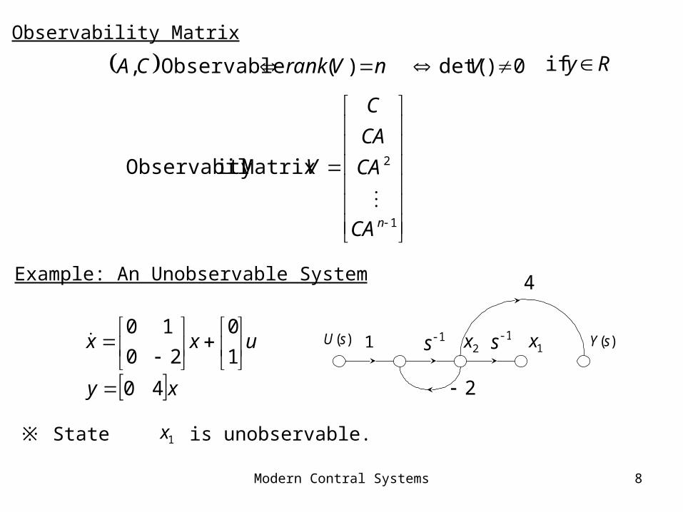
Example: An Unobservable System

xy

uxx

40

1

0

20

10

※ State is unobservable.1x

1)(sU -1s -1s 1x2x

2

4

)(sY

nVrankCA )(Observable , 0)det( V

1

2Matrix ity Observabil

nCA

CA

CA

C

V

Observability Matrix

Ry if


Proof of observability matrix

)1()2()3(11

1

)1()2(1321

1

111

111

1

)(),2(),1(

)(

)2()(

)1(

nknknkkkkkk

k

n

nknkkn

kn

kn

nk

kkkkkkk

kkk

kkk

kkk

DuCBuCABuDuCBuyDuy

x

CA

CA

C

n

nDuCBuBuCABuCAxCAy

DuCBuCAxDuBuAxCy

DuCxy

DuCxy

BuAxx

Inputs & outputs


10,1

0,

01

10

CBA

2)()( NrankVrank

01

10 ty Matrix Obervabili

01

10ix ility MatrControllab

CA

CN

ABBV

Example

DuCxy

RxBuAxx n

,

Plant:

Hence the system is both controllable and observable.


Theorem I

)()()( tuBtxAtx cccc

Controllable canonical form Controllable

Theorem II

)()(

)()()(

txCty

tuBtxAtx

oo

oooo

Observable canonical form Observable


example

c

cc

xy

uxx

12

1

0

32

10

Controllable canonical form

12

12

31

10

CA

CV

ABBU

nVrank

nUrank

1][

2][

o

oo

xy

uxx

10

1

2

31

20

Observable canonical form

31

10

11

22

CA

CV

ABBU

nVrank

nUrank

2][

1][

)2)(1(

2)(

ss

ssT


Theorem III

)()()(

)()()(

tDutCxty

tButJxtx

Jordan form

321

3

2

1

3

2

1

CCCC

B

B

B

B

J

J

J

J

Jordan block

Least row has no zero row

First column has no zero column

Linear system1. Analysis


Example

xccy

ub

b

xx

3

1100

020

012

1211

12

11

If 012 b uncontrollable

If 011 c unobservable


xy

uxx

2

1

0

203

102

200

201

101

211

100010

211

100010

001

000

1

1

1

2

2

2

1

1

1

1

11b

12b13b

21b

11C 12C 13C 21C


....

....

21131211

21131211

ILCILCCC

ILbILbbb

controllable

observable

In the previous example

....

....

21131211

21131211

DLCILCCC

ILbILbbb

controllable

unobservable


0

0

1

001

002

113

111

111

122

0

1

0

0

1

1001

123111

112

112

11

112

22

12

y

uxxL.I.

L.I.

L.I. L.D.

Example


zCy

uBzAz

m

mm

)0()0()( 111

nt

nt zevzevtz n

BuAxx DuCxy

Txz

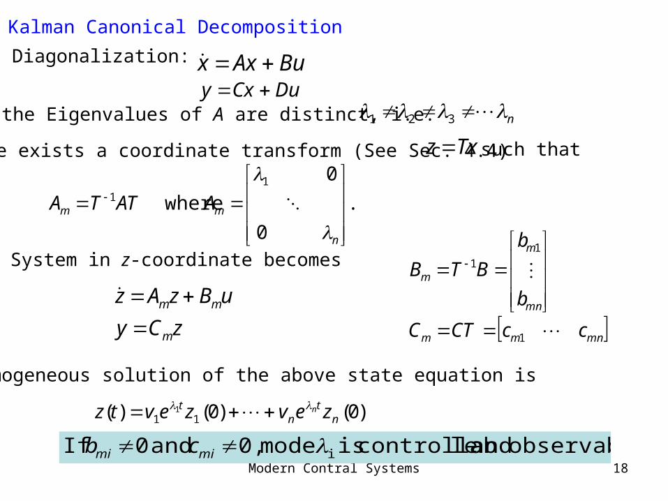
observable and lecontrollab is mode 0, and 0 If i mimi cb

Kalman Canonical Decomposition

Diagonalization:

There exists a coordinate transform (See Sec. 4.4)

n 321All the Eigenvalues of A are distinct, i.e.

such that

mnmm

mn

m

m

ccCTC

b

b

BTB

1

11

.

0

0

where1

1

n

mm AATTA

System in z-coordinate becomes

Homogeneous solution of the above state equation is


][ 21 n,v, , vvT

The coordinate matrix for diagonalization

t.independen are , rs,Eigenvecto 21 n,v, , vv

n 321All the Eigenvalues of A are distinct, i.e.

How to construct coordinate transformation matrix for diagonalization

ubzλz

ubzz

ubzz

mnnnn

m

m

2222

1111

nmnmm zczczcy 2211

Consider diagonalized system


n

mnmnmmn

i i

mimi

s

bc

s

bc

s

bcsH

1

11

1

)(

Transfer function is

le,unobservabor ableuncontroll is mode 0,or 0 If i mimi cb

H(s) has pole-zero cancellation.

1

1mc1mb

2

2mc2mb

n

mncmnb

∑

)(tu

)(ty


)(ty

OCS

COS

OCSOCS

)(tu

Kalman Canonical Decomposition

Subsystem ble Unobservale,Controllab:OCS

Subsystem Observable able,Uncontroll:OCS

Subsystem Observable le,Controllab :COS

Subsystem ble Unobservaable,Uncontroll:OCS


xCCy

uB

B

x

x

x

x

A

A

A

A

x

x

x

x

OCCO

OC

CO

OC

OC

OC

CO

OC

OC

OC

CO

OC

OC

OC

CO

00

0

0

000

000

000

000

Kalman Canonical Decomposition: State Space Equation

(5.X)


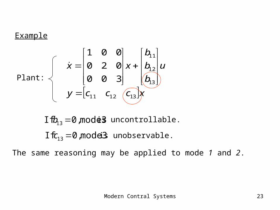
Example

xcccy

u

b

b

b

xx

311211

31

12

11

300

020

001

3 mode 0, If 13 b

3 mode 0, If 13 c

The same reasoning may be applied to mode 1 and 2.

Plant:

is uncontrollable.

is unobservable.


n

mnmnmmn

i i

mimi

s

bC

s

bC

s

bCsH

1

11

1

)(

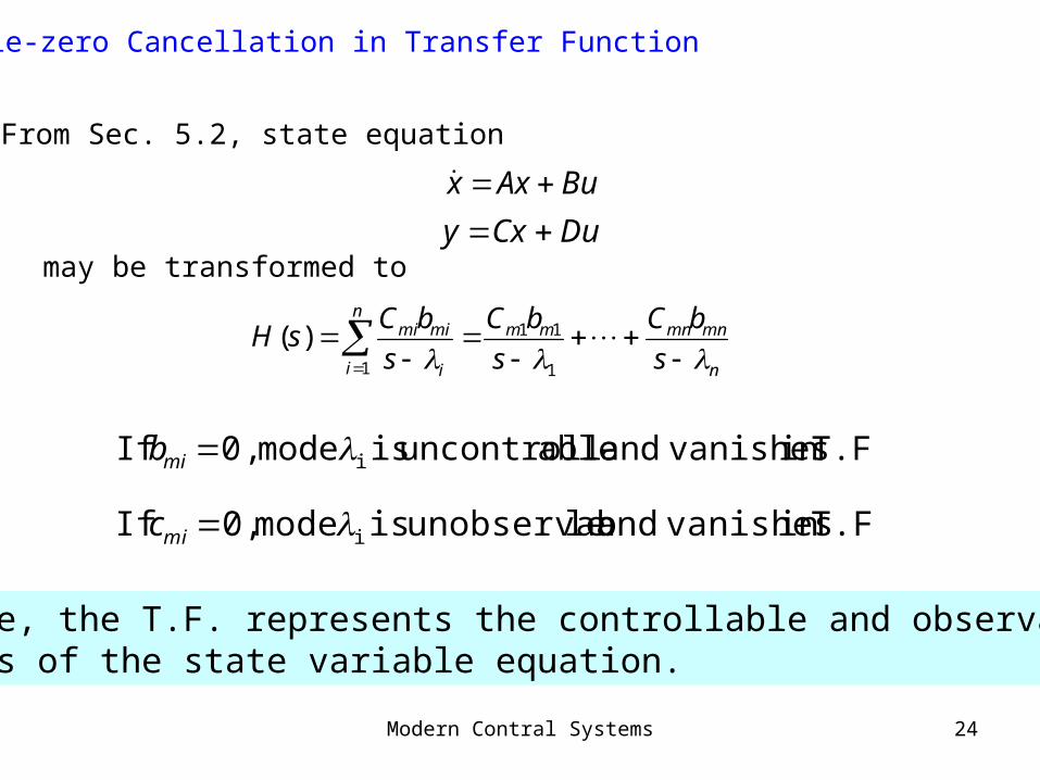
From Sec. 5.2, state equation

Hence, the T.F. represents the controllable and observableparts of the state variable equation.

may be transformed to

BuAxx

DuCxy

T.F.. in vanishesand ableuncontroll is mode , 0 If imib

T.F.. in vanishesand leunobservab is mode 0, If imic

Pole-zero Cancellation in Transfer Function


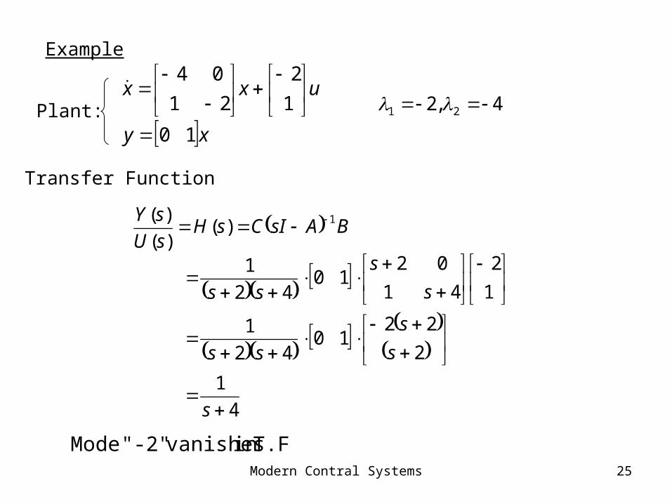
BAsICsHsU

sY 1)()(

)(

4

1

2

2210

42

1

1

2

41

0210

42

1

s

s

s

ss

s

s

ss

4,2 21

Example

xy

uxx

10

1

2

21

04

Transfer Function

T.F.. in vanishes"-2" Mode

Plant:


uxx

1

2

11

60

xy 10

3

1)(

)(

)( 1

sBAsICsT

sU

sY

Example 5.6

Plant:

Transfer Function

T.F.. in vanishes"2" Mode

-3,2 21


Minimum Realization

Realization: Realize a transfer function via a state space equation.

3

1)(

)(

)(

ssT

sU

sY

2

2

3

1)(

)(

)(

s

s

ssT

sU

sY

1 1)(sU )(sY

3

1 1)(sU )(sY-1s

3

2

-1s

-1s1

ExampleRealization of the T.F.

3

1)(

ssT

Method 1:

Method 2:

※There is infinity number of realizations for a given T.F. .


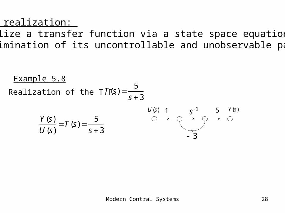
Minimum realization: Realize a transfer function via a state space equation with elimination of its uncontrollable and unobservable parts.

3

5)(

)(

)(

ssT

sU

sY1 5)(sU )(sY

3

-1s

Example 5.8

Realization of the T.F.3

5)(

ssT

modern contral systems1 lecture 06 analysis (ii) controllability and observability 6.1...

Documents

modern contral systemsfrom

state variable

state equationhence

state space equation5

transfer function6

given t

unobservable parts

rowfirst column