Numerical simulation of the 2011 Tohoku tsunami: Comparison with field observations and sensitivity tomodel parameters

Stephan T. Grilli1, Jeffrey C. Harris1, Tayebeh Tajalibakhsh1, James T. Kirby2, Fengyan Shi2

Timothy L. Masterlark3, and Christodoulos Kyriakopoulos1

(1) Department of Ocean Engineering, University of Rhode Island, Narragansett, RI, USA(2) Center for Applied Coastal Research, University of Delaware, Newark, Delaware, USA

(3) Department of Geological Sciences, The University of Alabama (UoA), Tuscaloosa, Alabama, USA(4) Instituto Nazionale di Geofisica e Vulcanologia, Rome, Italy

ABSTRACT

The March 11, 2011 M9 Tohoku-Oki Earthquake, which is believed to bethe largest event recorded in Japan history, created a majortsunami thatcaused numerous deaths and enormous destruction on the nearby Hon-shu coast. Various tsunami sources were developed for this event, basedon inverting seismic or GPS data, often using very simple underlyingfault models (e.g., Okada, 1985). Tsunami simulations withsuch sourcescan predict deep water and far-field observations quite well, but coastalimpact is not as well predicted, being over- or under-estimated at manylocations. In this work, we developed a new tsunami source, similarlybased on inverting onshore and offshore geodetic (GPS) data, but using3D Finite Element Models (FEM) that simulate elastic dislocations alongthe plate boundary interface separating the stiff subducting Pacific Plate,and relatively weak forearc and volcanic arc of the overriding Eurasianplate. Due in part to the simulated weak forearc materials, such sourcesproduce significant shallow slip along the updip portion of the rupturenear the trench (several tens of meters).

We assess the accuracy of the new approach by comparing nu-merical simulations to observations of the tsunami far- andnear-fieldcoastal impact, using: (i) one of the standard seismic inversion sources,which we found provided the best prediction of tsunami near-field im-pact in our model (UCSB; Shao et al. (2011)); and (ii) the new FEMsource. Specifically, we compare numerical results to DART buoy, GPStide gage, and inundation/runup measurements. Numerical simulationsare performed using the fully nonlinear and dispersive Boussinesq wavemodel FUNWAVE-TVD, which is parallelized and available in Cartesianor spherical coordinates. We use a series of nested model grids, withvarying resolution (down to 250 m nearshore) and size, and assess effectson results of the latter and of model physics (such as when including dis-persion or not). We also assess effects of triggering the various tsunamisources in the propagation model: (i) either at once as a hot start, orwith the spatio-temporal sequence derived from seismic inversion; and(ii) as a specified surface elevation or as a more realistic time and space-varying bottom boundary condition (in the latter case, we compute theinitial tsunami generation up to 300 s using the non-hydrostatic modelNHWAVE).

Although additional refinements are expected in the near future, re-sults based on the current FEM sources better explain near field observa-tions at DART and GPS buoys near Japan, and measured tsunami inun-dation, while they simulate observations at distant DART buoys as wellor better than the UCSB source.

KEYWORDS: Tsunami source modeling; Tsunami propagationmodeling; Boussinesq model; Wave dispersion effects.

INTRODUCTION

On March 11th, 2011, at 2:46 pm JST, a magnitudeMw = 9.0 earth-quake struck near the northeastern coast of Japan (37◦49’ N, 143◦03’ E;Fig. 1), with substantial slip at fairly shallow depths (about 10-20 km),causing large seafloor motions that triggered very high tsunami waves,perhaps the largest in Japan’s recorded history. The main earthquakeshocks lasted for 3-4 minutes and, owing to the proximity of the epi-center to shore, the first significant waves reached Japan only 10 minutesafter the event started, thus allowing for very little warning time. Thetsunami caused extensive destruction along the coast of theTohoku re-gion, between 35◦ - 43◦ N. Post-tsunami surveys reported maximum ofrunups and inundation depths values in the 20-40 m range, mostly be-tween 37.7◦ - 40.2◦ N where the Miyagi and Iwate Prefectures are lo-cated (The 2011 Tohoku Earthquake Tsunami Joint Survey Group, 2011;Mori et al., 2011a). The largest runups occurred in the north, along theSanriku/Ria coast (north of 37◦ N), which has a very complex topogra-phy that amplifies tsunami impact. By contrast, areas located directlysouth, which mostly consist of plains, were less impacted. As a result ofthe tsunami, nearly 16,000 people lost their lives and 4,000were reportedmissing; many were injured and millions more were affected by the lackof water and food, electricity, and transportation (IOC/UNESCO, 2011).

Within one hour of the event, when the tsunami reached the nearestDART buoys (Deep-water Assessment and Reporting of Tsunaminet-work; Gonzalez et al. (1998); Fig. 1), propagation models ofthe antici-pated far-field impact caused sufficient concern to trigger evacuations andwarnings in many distant areas across the Pacific Ocean. Large impactwas predicted as far as Chile, where waves were expected to arrive af-

8 cm/yr

0 1000500 1500-1000 -500-1500

2500

3500

4500

5500

3000

4000

5000

UTM km east

UT

M k

m n

ort

h

Pacific Ocean

Pacific

Plate

Okhotsk

Plate

Sea of Japan

Philippine

Sea Plate

J AP

AN

Sendai

model domain

Japan

Tre

nch

Amur

Plate

Oki

nawa

Pla

teYangtze

Plate

Eurasian

Plate

0

2000

4000

-8000

-2000

-4000

-6000ele

vation m

sl, m

UT

M z

one 5

4

UT

M z

one 5

3

Miyagi, and Fukushima.

Fig. 1: M9 2011 Tohoku earthquake seismotechtonics (rupture zonemarked by red polygon). Large symbol is the epicenter; yellow dots showM > 4 aftershocks (11 March 06 May 2011). The Pacific-Okhotsk plateconvergence is about 8 cm/yr. Black diamonds mark coastal GPS wavebuoys (Yamazaki et al., 2011a).

ter more than 20 h of propagation. In the meantime, through a chain offailures of coastal protections and back-up power systems caused by theearthquake and the tsunami inundation, the core of one of thereactorsat the Fukushima Dai-Ichi nuclear power plant (near 37◦ 25’ N) startedmelting, eventually causing explosions that released large doses of radia-tion, forcing a complete evacuation in the days following the event of allpeople living within tens of kilometers of the power plant that will likelylast for many decades.

The earthquake ruptured the boundary separating the subducting Pa-cific Plate from the overriding Okhotsk Plate; this segment of the plateboundary intersects the seafloor at the Japan Trench (Fig. 1), where itdips about 10◦ to a down-dip distance of about 100 km from the trench.The rupture area, 150 km east of Sendai, Japan, extends a few hundredkm in the along strike direction, offshore of the Prefectures of Aomori,Miyagi, and Fukushima. At the latitude of the earthquake, the PacificPlate moves approximately westwards with respect to the Okhotsk Plateat a rate of 8 cm/yr (DeMets et al., 1994) (Fig. 1). The focal mechanismsreported by Harvard CMT, the U.S. Geological Survey (USGS),and theEarthquake Research Institute at the University of Tokyo, all indicatedthat the earthquake was predominantly thrust with a moment more thanMo ≃ 4.0 × 10

22 N.m and a variety of seismic, geodetic, and tsunamigenesis studies concluded that the magnitude was indeedMw = 9.0

(e.g., Ide et al. (2011)). Some geodetic inversion models (e.g., Ozawaet al. (2011); Pollitz et al. (2011)) suggest that the peak slip may haveexceeded 30-35 m in some areas, while some seismic inversionmodelssuggest over 50-60 m of maximum slip (e.g., Ammon et al. (2011); Shaoet al. (2011); Lay et al. (2011a)). Owing to the small dip angle, suchlarge slip values caused very large uplift of the seafloor, likely reachingwell over 10 m in a large central area of the tsunami source (Fig. 1).

MODELING OF THE TOHOKU-OKI CO-SEISMIC SOURCE

Since the Tohoku event, a large variety of seismic models of the earth-quake have been proposed. These were usually based on inverting seis-mic and/or geodetic data, using the Okada (1985) model, which assumesa superposition of planar dislocations (i.e., finite faults) embedded in ho-mogeneous elastic half-spaces (HEHS), or a similarly idealized source

model of the subduction zone (e.g., Dziewonski’s 1981 spherical layeredPREM seismological model; see, e.g., Ammon et al. (2011); GeospatialInformation Authority of Japan (2011); Pollitz et al. (2011); Ozawa et al.(2011); Shao et al. (2011)). One of these seismic inversion sources, re-ferred to as UCSB (Shao et al., 2011), will be used in this study (seedetails below).

(a) (b)

Fig. 2: Computational domains for FUNWAVE-TVD simulations: (a)near-field (regional 1000 m and coastal 250 m, large/small red boxes)Cartesian grid (also for NHWAVE); and (b) far-field (Pacific basin scale)4’ spherical grid, with marked location of 18 DART buoys (yellow/reddots). White dots in (a) indicate locations of the GPS buoys of Fig. 1

In the present work, to better account for the actual geometry ofthe Japan trench and its forearc, as well as inhomogeneitiesin materialproperties in the subduction zone (e.g., weaker forearc andstiffer sub-ducting plate materials), we developed and used our own source, basedon a more comprehensive and detailed Finite Element Modeling (FEM)(Masterlark, 2003) of the subduction zone near Japan. An earlier im-plementation of this approach was successfully applied to the 2004 M9Sumatra-Andaman earthquake (Masterlark and Hughes, 2008). This newtsunami source (referred to as University of Alabama; UA) was devel-oped by inverting onshore and offshore geodetic data but, rather thanusing Okada’s idealized HEHS solution, it used 3D FEMs to simulateelastic dislocations along the plate boundary interface separating the stiffsubducting Pacific Plate, and relatively weak forearc and volcanic arc ofthe overriding Eurasian plate. Details are given below.

Another aspect of co-seismic sources that affects tsunami simu-lations in a propagation model is whether one triggers the maximumseafloor deformation at once, as a hot start in the model, for the entiresource area, or triggers sub-areas of the source as a time sequences thatmimics the actual earthquake event. Such a time sequence canbe ob-tained as a result of seismic inversion methods. In this event, seismicinversion models (e.g., Harvard CMT) show that the main earthquakelasted for 3-4 minutes, during which tsunami waves may have propagateda large distance towards Japan. Hence, in the present case, it is importantto trigger waves as a function of time and resolve interferences (construc-tive or destructive) that may have resulted. The sensitivity of tsunamigeneration to this timing aspect will be studied in the present work. Ad-ditionally, we will study the sensitivity of results to the way the tsunamiis initially specified in the propagation model: (i) either as a free surfaceelevation with no initial velocity (as it is customary to do in most studiesowing to the near incompressibility of water and small rise times); (ii)or as a more realistic time dependent bottom boundary condition (in thiscase a different type of model, NHWAVE, that allows for such abound-ary condition will first be used during 300 s, before moving results into along wave propagation model; this is detailed later).

(a) (b)

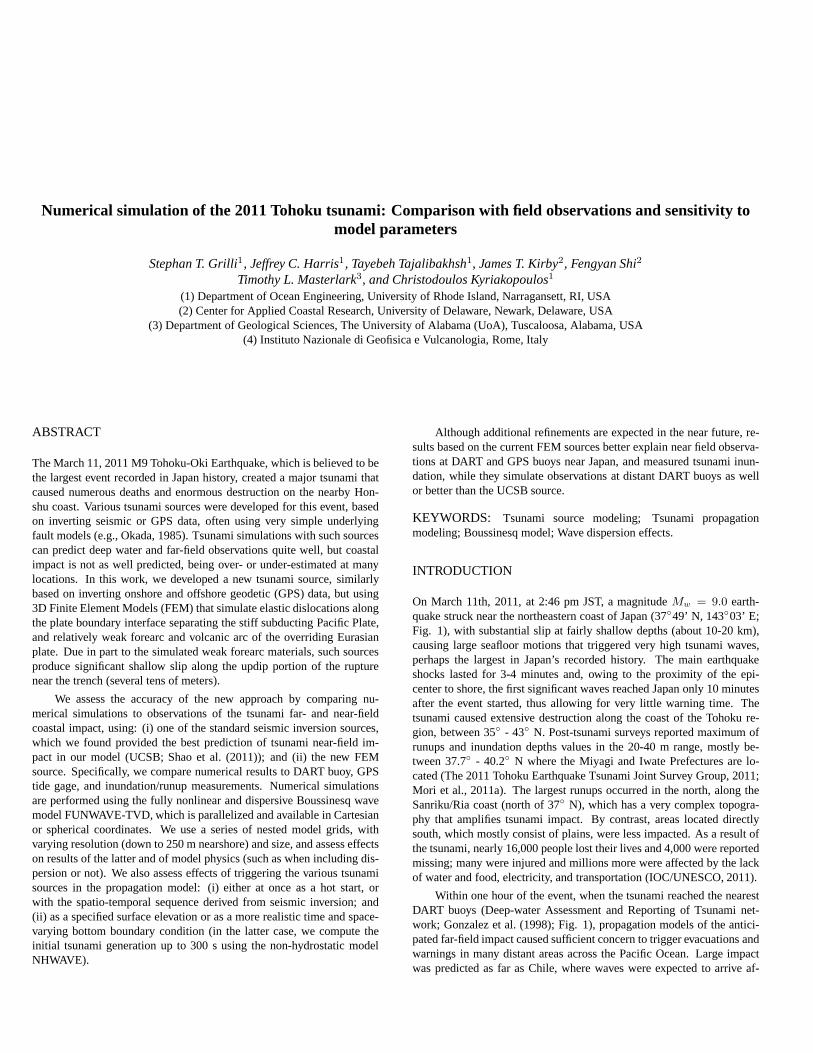
Fig. 3: UCSB source (Shao et al., 2011): (a) Source area and maximumslip distribution; and (b) vertical seafloor displacement.

UCSB source

The source we denote as UCSB is based on the slip history derived byShao et al. (2011) using tele-seismic body and surface seismic waves.It assumes, the earthquake epicenter was located at 38.10◦ N and142.86◦ E, and the seismic moment wasMo = 5.84 × 10

22 N.m, fora dip angle of 10◦ and a strike angle of 198◦. Fig. 3 shows the maximumslip distribution obtained for this source, as well as the correspondingmaximum vertical seafloor displacement.

UA source

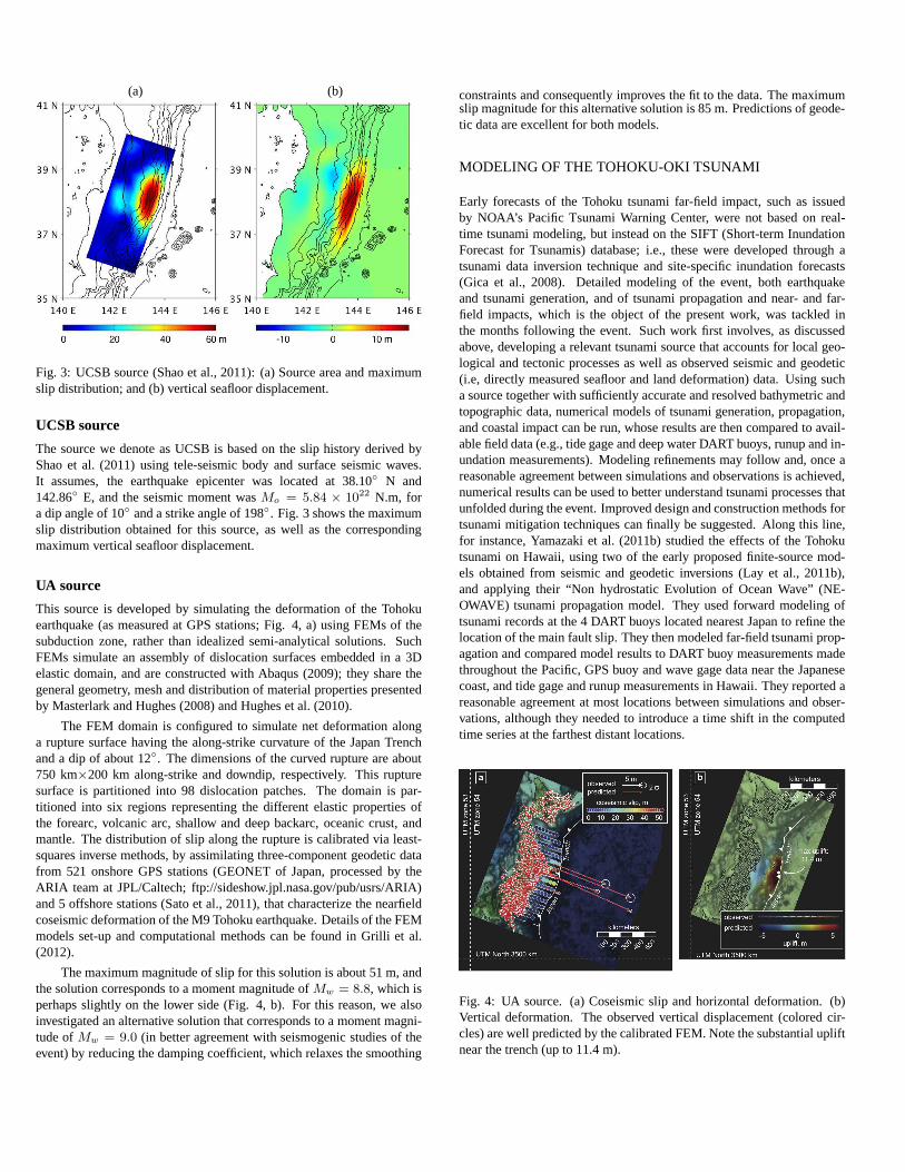
This source is developed by simulating the deformation of the Tohokuearthquake (as measured at GPS stations; Fig. 4, a) using FEMs of thesubduction zone, rather than idealized semi-analytical solutions. SuchFEMs simulate an assembly of dislocation surfaces embeddedin a 3Delastic domain, and are constructed with Abaqus (2009); they share thegeneral geometry, mesh and distribution of material properties presentedby Masterlark and Hughes (2008) and Hughes et al. (2010).

The FEM domain is configured to simulate net deformation alonga rupture surface having the along-strike curvature of the Japan Trenchand a dip of about 12◦. The dimensions of the curved rupture are about750 km×200 km along-strike and downdip, respectively. This rupturesurface is partitioned into 98 dislocation patches. The domain is par-titioned into six regions representing the different elastic properties ofthe forearc, volcanic arc, shallow and deep backarc, oceanic crust, andmantle. The distribution of slip along the rupture is calibrated via least-squares inverse methods, by assimilating three-componentgeodetic datafrom 521 onshore GPS stations (GEONET of Japan, processed bytheARIA team at JPL/Caltech; ftp://sideshow.jpl.nasa.gov/pub/usrs/ARIA)and 5 offshore stations (Sato et al., 2011), that characterize the nearfieldcoseismic deformation of the M9 Tohoku earthquake. Detailsof the FEMmodels set-up and computational methods can be found in Grilli et al.(2012).

The maximum magnitude of slip for this solution is about 51 m,andthe solution corresponds to a moment magnitude ofMw = 8.8, which isperhaps slightly on the lower side (Fig. 4, b). For this reason, we alsoinvestigated an alternative solution that corresponds to amoment magni-tude ofMw = 9.0 (in better agreement with seismogenic studies of theevent) by reducing the damping coefficient, which relaxes the smoothing

constraints and consequently improves the fit to the data. The maximumslip magnitude for this alternative solution is 85 m. Predictions of geode-tic data are excellent for both models.

MODELING OF THE TOHOKU-OKI TSUNAMI

Early forecasts of the Tohoku tsunami far-field impact, suchas issuedby NOAA’s Pacific Tsunami Warning Center, were not based on real-time tsunami modeling, but instead on the SIFT (Short-term InundationForecast for Tsunamis) database; i.e., these were developed through atsunami data inversion technique and site-specific inundation forecasts(Gica et al., 2008). Detailed modeling of the event, both earthquakeand tsunami generation, and of tsunami propagation and near- and far-field impacts, which is the object of the present work, was tackled inthe months following the event. Such work first involves, as discussedabove, developing a relevant tsunami source that accounts for local geo-logical and tectonic processes as well as observed seismic and geodetic(i.e, directly measured seafloor and land deformation) data. Using sucha source together with sufficiently accurate and resolved bathymetric andtopographic data, numerical models of tsunami generation,propagation,and coastal impact can be run, whose results are then compared to avail-able field data (e.g., tide gage and deep water DART buoys, runup and in-undation measurements). Modeling refinements may follow and, once areasonable agreement between simulations and observations is achieved,numerical results can be used to better understand tsunami processes thatunfolded during the event. Improved design and construction methods fortsunami mitigation techniques can finally be suggested. Along this line,for instance, Yamazaki et al. (2011b) studied the effects ofthe Tohokutsunami on Hawaii, using two of the early proposed finite-source mod-els obtained from seismic and geodetic inversions (Lay et al., 2011b),and applying their “Non hydrostatic Evolution of Ocean Wave” (NE-OWAVE) tsunami propagation model. They used forward modeling oftsunami records at the 4 DART buoys located nearest Japan to refine thelocation of the main fault slip. They then modeled far-field tsunami prop-agation and compared model results to DART buoy measurements madethroughout the Pacific, GPS buoy and wave gage data near the Japanesecoast, and tide gage and runup measurements in Hawaii. They reported areasonable agreement at most locations between simulations and obser-vations, although they needed to introduce a time shift in the computedtime series at the farthest distant locations.

Fig. 4: UA source. (a) Coseismic slip and horizontal deformation. (b)Vertical deformation. The observed vertical displacement(colored cir-cles) are well predicted by the calibrated FEM. Note the substantial upliftnear the trench (up to 11.4 m).

Summary of tsunami generation and propagation models

Large co-seismic tsunamis have usually been simulated using (non-dispersive) Nonlinear Shallow Water (NSW) wave equation models (e.g.,Kowalik and Murty (1993)). By contrast, the more dispersivelandslidetsunamis have been simulated with Boussinesq models (BM), or simi-lar models, which are nonlinear and dispersive (Watts et al., 2003; Dayet al., 2005; Tappin et al., 2008). More recently, however, dispersive mod-els such as BMs have also been increasingly used to simulate co-seismictsunamis (Grilli et al., 2007, 2010; Ioualalen et al., 2007;Karlsson et al.,2009). Although dispersive effects may not always be significant in longtsunami wave trains, when they are called for, BM equations feature themore extended physics required for simulating such effects; Ioualalenet al. (2007), for instance, showed differences in the computed elevationof leading waves, for the 2004 Indian Ocean tsunami event near Thailand,of up to 30% when simulating the tsunami using a BM with or withoutthe dispersive terms.

We model the Tohoku event using the BM model FUNWAVE, whichwas initially developed and validated for coastal wave dynamics prob-lems (Wei et al., 1995; Chen et al., 2000, 2003; Kennedy et al., 2000); thismodel was later used to perform tsunami case studies (e.g., Ioualalen et al.(2007)). In its most recent implementation, FUNWAVE-TVD, in Carte-sian (Shi et al., 2012) or spherical coordinates with Coriolis effects (Kirbyet al., 2009, 2012), the code uses a TVD shock-tracking algorithm thatmore accurately simulates wave breaking and inundation. Earlier workshows that the numerical diffusion resulting form the TVD scheme yieldsan accurate representation of wave height decay in the surfzone (Shiet al., 2012). For tsunamis, FUNWAVE-TVD has been validatedagainst alarge set of analytical, laboratory, and field benchmarks (Tehranirad et al.,2011) as part of the development of tsunami hazard maps for the US EastCoast. Because of their more complex equations, BMs are typically morecomputationally demanding than NSW models. For this reason, an opti-mized MPI parallel implementation of FUNWAVE-TVD was developed,which has highly scalable algorithms with a typical acceleration of com-putations of more than 90% the number of cores in a computer cluster(Shi et al., 2012). This makes it possible running the model over largeocean basin-scale grids, with a sufficiently fine resolution. Present re-sults will show that dispersive effects are not significant in the near-fieldfor the type of tsunami sources used to date. However, as these sourcesare refined (both in space and time) to include more complex geologicalprocesses (e.g., sub-faults and splay faults), one will increasingly haveto model the superposition and interactions of shorter and hence moredispersive waves, which requires using models that simulate this type ofphysics (such as BMs).

To specify and study effects of time-dependent tsunami sources trig-gered by transient motion of the seafloor (which is not a feature ofFUNWAVE-TVD), the non-hydrostatic model NHWAVE developedbyMa et al. (2012) will be used to compute the initial tsunami generation(up tot = 300 s). NHWAVE provides a numerical solution of the three-dimensional Navier Stokes equations for incompressible flows, in aσ

coordinate framework (typically with 3 levels), but with the simplify-ing assumption of a single-valued water surface displacement. Ma et al.(2012) have validated the model performance for landslide tsunami gen-eration by comparing to the highly dispersive laboratory data presentedby Enet and Grilli (2007). FUNWAVE-TVD or NHWAVE are initializedwith either the USCB or the new UA source. Once generated, we simu-late the near-field tsunami propagation from the source to the Japan coastin FUNWAVE-TVD’s Cartesian implementation and the far-field tsunamipropagation from the source to distant locations in the Pacific Ocean inits spherical implementation. Fig. 2 shows the ocean-basinscale domain

(with 4’ arc mesh (b); spanning 132◦ E to 68◦ W and 60◦ S to 60◦ N)used for the far-field propagation computations, and the more finely re-solved regional grid (with 1000 m mesh (a) large; 800 by 1200 km), en-compassing both the earthquake source and the Japan coastline, used forcomputing near-field tsunami impact. Finally, runup and inundation sim-ulations are done in a smaller coastal grid (with 250 m mesh (a) small).Earth’s sphericity is corrected in Cartesian coordinates with a transversesecant Mercator projection with its origin located at (39◦ N, 143◦ E). Thistransformation leads to small grid distortions, which are deemed negligi-ble.

In all (FUNWAVE or NHWAVE) simulations, free-slip (wall)boundary conditions are applied on solid lateral boundaries. To preventnon-physical reflection from these boundaries, sponge layers are speci-fied over a number of grid cells to absorb outgoing waves (inside of theouter domain boundary marked in Fig. 2), for which damping terms areactivated in the model equations. For the Pacific grid, sponge layers are100 km thick along all lateral boundaries and, in the regional grid, theyare 50 km thick in the north and south ends of the domain, and 200 kmthick in the east. Finally, in the 250 m coastal grids, spongelayers are 50km thick along the north, east and south boundaries.

FIELD DATA

Many tsunami observations were made during and after the event. Forcomparison with model simulations and validations, we willuse: (i) deepwater DART buoy measurements of surface elevation (Lay et al., 2011b);(ii) nearshore GPS buoy or tide gauge measurements of surface elevation(Yamazaki et al., 2011a); and (iii) onshore runup and inundation height(The 2011 Tohoku Earthquake Tsunami Joint Survey Group, 2011; Moriet al., 2011a,b).

The latter data was recorded at more than 5,300 individual locationsduring post-event surveys conducted by a large international team of sci-entists, along a 2,000 km stretch of the Japanese. Inundation heightswere obtained from watermarks on trees, walls, and buildings, and de-tided for the time of tsunami impact. Run-up heights were derived fromthe maximum extent of debris deposits and water marks. DART buoydata is routinely collected in 15 s to 15 minute intervals, depending onthe level of alert. When the passage of a tsunami has been identified ata particular buoy (after the DART network has been put on alert), aver-age surface elevation data is transmitted every 15 s during the initial fewminutes, followed by 60 s intervals (Gonzalez et al., 1998).To obtainthe tsunami signal, this data first needed to be filtered to remove the tidalsignal (Butterworth filter) and it was then interpolated to get equal inter-vals of 15 s. DART buoys used here are labeled in Fig. 2. A series ofmoored GPS-mounted buoys from the NOWPHAS (Nationwide OceanWave information network for Ports and HArbourS; http://nowphas.mlit.go.jp/infoeng.html) moored near the Japan coast (in water depth of 100to 300 m and at a distance of 10 to 20 km from the coastline; Fig.1)resisted the large tsunami waves. After applying a low-passfiltering witha moving average technique, these provided time series of surface eleva-tion.

Bathymetric and topographic data used in modeling was com-pounded from: the 1’ arc resolution ETOPO1 database, the 500m res-olution J-EGG500 bathymetry (JODC-Expert Grid data for Geography)along the Japanese coastline, and the 1 arc-second ASTER topographicdata. In deep water, only ETOPO1 data was used while for the re-gional/coastal grids, the other (finer) data sources were used wheneveravailable. Data from various sources was linearly interpolated.

(a) (b) (c)

(d)

Fig. 5: Sensitivity of initial tsunami elevation computed at t = 300 s tothe initialization method, for the UCSB co-seismic source :(a) instan-taneous triggering on the free surface in FUNWAVE-TVD, withmaxi-mum seafloor displacement; (b) time-varying triggering on the free sur-face in FUNWAVE-TVD, with instantaneous seafloor displacement; and(c) time-varying seafloor displacement specified as a boundary conditionin NHWAVE. Black lines indicate locations of transect used in (d), andthe black dot is the origin of the axis in the latter figure. (d)transect inresults for method : (—) (a); (– – –) (b); (– - –) (c).

RESULTS

As indicated, we simulate the propagation of the Tohoku 2011tsunamiacross the Pacific Ocean, and its coastal transformations, runup and inun-dation along the Japanese coastline, in a series of computational domains(Fig. 2). All numerical simulations begin with 300 s of computations ofthe initial tsunami waveform in the 500 by 800 km, 1000 m resolution, re-gional grid, in which we first study the sensitivity of results to whether theco-seismic tsunami sources are triggered at once or in a timesequence inthe propagation model. In the latter case, we also verify whether it is rel-evant to linearly superimpose non-moving free surface elevations, whentriggering large tsunami waves in a time sequence.

Results at 300 s (or 5 mins.) are then interpolated, through aone-way coupling, from the regional grid onto one of two FUNWAVE-TVDgrids (Table 1): either (i) directly on the 4’ arc spherical grid for far-fieldtranspacific simulations; or (ii) following an additional 10 min. of propa-gation in the 1000 m FUNWAVE grid, onto the 250 m resolution coastalCartesian grid (in order to both get the westward propagating waves tofully enter the 250 m grid and separate these from the eastward prop-agating wave), to perform all near-field simulations. The latter includecomputations of time series at GPS tide buoys as well as computations ofrun-up and inundation along the coast.

Result sensitivity to initialization method

Three types of initializations are tested and compared in the regionalgrid for the UCSB co-seismic source shown in Fig. 3: (1) a hot startof FUNWAVE-TVD as a free surface elevation without initial velocity,by either (a) specifying the maximum seafloor vertical displacement atonce (e.g., such as in Fig. 3, or (b) as a time-dependent triggering; (2)as a time-dependent bottom boundary condition in NHWAVE. Fig. 5shows the computed free surface elevations att = 300 s and a transect in

those, for these three cases. Significant differences can beseen, in bothsurface elevation and wavelength, between the instantaneous method (1a)and the two time-dependent methods (1b,2). Smaller differences can thenbe observed between the latter two methods, with the time-triggering inNHWAVE resulting in slightly reduced maximum (positive or negative)elevations and in waveforms with less higher-frequency oscillations thanfor the time-triggering in FUNWAVE-TVD. This might be due tothe ad-justment of the solution kinematics to the non-physical superposition offree surface increments with no initial velocity. Overall,these resultsjustify using the 3rd more accurate and realistic method to compute theinitial tsunami waveform, which will be done in all the following compu-tations.

Fig. 6: Surface elevations (m) as a function of time (h), at some of theGPS buoys from N to S (Figs. 1), at: (a) North Iwate; (b) Central Iwate;(c) South Iwate; (d) North Miyagi; (e) Central Miyagi. Each panel com-pares observations (black) to computations for the : UCSB (M9) source(blue) and UA (M8.8) source (red).

Surface elevation at coastal GPS buoys

Fig. 6 compares surface elevations simulated at some GPS buoys withthe UCSB and UA sources, to observations. Overall, the agreement isgood for both sources. Although neither source matches the data as well

Fig. 7: Surface elevation (m) as a function of time (h) at DARTbuoys(Fig. 2) #: (a) 21413; (b) 21418; (c) 21401; (d) 21419; (e) 51407(+6.6 min); (f) 46404 (+7.2 min). Comparison between observations(black) and computations with FUNWAVE-TVD using the : UCSBsource (blue); and the UA source (red).

for the first 3 northern buoys (a-c), than further south (d-e), results ofthe UA source seem in better agreement with observations than those ofthe UCSB source, when considering the whole waveform. Note that ourfindings for the UCSB source results are somewhat similar to those ofYamazaki et al. (2011b), which show generally good agreement with thebuoy data, but for some stations (i.e., North and Central Miyagi) theirsimulations underpredict the observed amplitude, and for others (i.e.,South Miyagi, not shown here, which they refer to as the Fukushima GPSstation) they overpredict the initial amplitude.

Trans-Pacific propagation and dispersive effects

Simulation were run for 24 hours of tsunami propagation, in order forwaves to reach the most distant DART buoys and the South Americancoastline. Figs. 7, a-d shows a comparison of computed surface ele-vations with the UCSB and UA sources, and measurements at thefourDART buoys closest to Japan (i.e., No. 21413, 21418, 21401, and 21419;Fig. 2). Overall, results for both the UCSB and UA sources agree wellwith observations. The UCSB source, however, consistentlyoverpredictsthe leading wave crest elevation at each location and, more notably, over-predicts the amplitude of the leading wave troughs. Both theUA andUCSB sources predict that the wave arrives slightly sooner than seen inobservations, but this is more pronounced for the UCSB source. Figs. 7,e,f similarly show a comparison of computed and measured surface ele-vations at two distant DART buoys, in Hawaii and of of Oregon (i.e., No.51407, 46404; Fig. 2). Similar to Yamazaki et al. (2011b), wefind thatthe tsunami arrives earlier than observed (about 7 mins). Hence, to allowfor an easier comparison, slight time shifts have been addedto simula-tions in the figure, in order to synchronize the first elevation wave withthat observed. These only represent about 1.5% of the tsunami propa-gation time and can be explained in part by a combination of grid andbathymetric resolution effects, as well as slight errors inthe source lo-cation and triggering. Additional systematic errors on propagation timescould results from the fact that the Earth is not perfectly spherical. [Forthese simulations, we assumed an earth radius of 6,371 km.] The pre-dicted surface elevations at distant DART buoys generally agree reason-ably well with observations and, at buoy (f), the UA source matches theleading wave much better than the UCSB source.

Figure 8, a shows the envelope of computed maximum wave ele-vation (for the UCSB source). We see, the tsunami energy propagatesacross the ocean in some preferential directions, associated with both thesource characteristics and the ocean bathymetry, in which ridges maycause wave-guiding effects. This is particularly clear forthe eastwardpropagation towards Northern California, around 40◦ N; large wave os-cillations (nearly 4 m trough to crest) and damage were indeed observedat this latitude in Crescent City, CA. Frequency dispersioneffects on thispropagation are assessed by re-running these simulations without disper-sion terms in FUNWAVE-TVD’s equations (i.e., in NSW mode). Figure8, b shows a difference plot between results with and withoutdispersion.As could be expected from the short propagation distances and the coarsegrid resolution, little dispersive effects can be seen in the near field, closeto Japan. In the far-field, however, non-negligible differences with NSWresults, of more than±10 cm, can be seen in deep water, which mayamount to 20-40% of the tsunami amplitude at some locations.This ison the same order of magnitude as that of dispersive effects reported byIoualalen et al. (2007) for the 2004 Indian Ocean tsunami andjustifiesusing a BM in the present case. A more detailed discussion andanalysisof dispersive effects and their comparison to Coriolis force effects for theTohoku 2011 event can be found in Kirby et al. (2012).

Runup and inundation

After 300 s of simulations in the regional grid, the tsunami is simulatedfor another 2 hours in the coastal grid. Both runup and inundation dataare available from the field surveys. In order to accurately predict runup,however, particularly in the north along the Sanriku/Ria coast (39.5◦ and40.25◦ N), which has a very complex topography that could greatly en-hance it, one needs to use a much finer model grid than 250 m (perhapsdown to 20-30 m resolution). This would also require using a better re-solved bathymetry than the 500 m data set currently used. Hence, with thecurrent grid resolution, we believe a comparison with inundation resultsis more realistic than runup, as inundation is predicted at the shoreline.This is done in Fig. 9, where computed inundations for both sources are

(a)

(b)

Fig. 8: (a) Maximum wave elevation computed with FUNWAVE-TVDin the spherical (4’) Pacific grid for the UCSB source. (b) Differencebetween (a) and a (non-dispersive) NSW simulation of the same case.

directly compared to observed inundation values, north of 36◦ N. In thisregion, results for the UA source are found in good agreementwith obser-vations, except between 39.1◦ and 40.2◦ N, where these are significantlyunderpredicted in the model. By contrast, as already seen atsome GPSand nearsore DART buoys, the UCSB source significantly overpredictsthe observed inundation from 38.25◦ to 39.7◦ N (and thus the correspond-ing seafloor deformation offshore) and, like the UA source, underpredictsthe inundation between 39.7◦ and 40.2◦ N, albeit by a smaller factor.Overall, based on these results, the UA source is seen to agree better withtsunami observations.

SUMMARY

We simulated tsunami generation propagation, near-field (coastal), andfar-field impact of the Tohuku 2011 tsunami and compared results to fieldobservations of surface elevation at DART buoys, GPS gage buoys, andrunup and inundation along the most impacted coastal area ofJapan (from35◦-41◦ N). Our BM model was initialized based on co-seismic tsunamisources developed from seismic (UCSB; Shao et al. (2011)) orGPS data(UA) inversion based on a detailed FEM of the subduction zone. Resultsshowed that dispersive effects are negligible in the near-field, but mayaccount for 20-40% of tsunami amplitude in deep water, hencejustifyingthe use of a Boussinesq model. The sensitivity of results to three sourcetriggering methods was assessed for the UCSB co-seismic source. Re-sults justified using the 3rd more accurate and realistic method with atime dependent bottom boundary condition in NHWAVE, to compute theinitial tsunami waveform.

Salient features of the observed tsunami far-field and coastal impactwere well reproduced for both sources, but coastal impact was over- orunder-estimated at some locations. Overall, however, results obtainedfor the UA source were found in better agreement with observations atnearshore GPS gages and DART buoys, and at some distant DART buoys,than those for the UCSB source. It was found that both sourcesaccuratelypredicted inundation observations south of 38◦ N. To the north, results forthe UA source were found in good agreement with observations, exceptbetween 39.7◦ and 40.2◦ N, where they were underpredicted. In additionto the complex coastline mentioned above, this is an area where the UAsource may lack in tsunami generation, perhaps due to underpredictedseafloor deformations; but this could also be due to other phenomena notincluded in the co-seismic sources (e.g., splay faults, underwater land-slides,...). In fact, there were early indications that Submarine Mass Fail-ures (SMFs) may have been triggered in the Japan trench by theTohoku-Oki M9 earthquake (Fujiwara et al., 2011). By contrast, the UCSB sourcesignificantly overpredicted observed inundations up to 39.7◦ N and, likethe UA source, underpredicted inundation between 39.7◦ and 40.2◦ N,albeit by a smaller factor.

Overall, the UA source was thus found to agree better with tsunamiobservations, in both the near- and far-field, than those using the UCSBsource, although it may need additional refinements to better explain ob-servations between 39.7◦ and 40.2◦ N; these are currently in developmentand expected to be available in the near future.

Fig. 9: Tsunami inundation measured (black dots) and computed (red)with: (a) M9 UCSB source; and (b) M8.8 UA source.

ACKNOWLEDGEMENTS

The first 3 and last 2 authors acknowledge support from grant EAR-09-11499/11466 of the US National Sciences Foundation (NSF) GeophysicsProgram. JT and FS acknowledge the Coastal Geosciences Program, Of-fice of Naval Research for support for development of the FUNWAVE-TVD and NHWAVE models.

REFERENCES

Abaqus (2009).Abaqus. Dassault Systemes Simulia Corp., Providence, RI, 6.9-EFedition.

Ammon, C. J., Lay, T., Kanamori, H., and Cleveland, M. (2011). A rupture modelof the great 2011 Tohoku earthquake.Earth Planets Space, (accepted):4 pp.

Chen, Q., Kirby, J. T., Dalrymple, R. A., Kennedy, A. B., and Chawla, A. (2000).Boussinesq modeling of wave transformation, breaking and runup. II: Two hor-izontal dimensions.J. Waterway, Port, Coastal and Ocean Engrng., 126:48–56.

Chen, Q., Kirby, J. T., Dalrymple, R. A., Shi, F., and Thornton, E. B. (2003).Boussinesq modeling of longshore currents.Journal of Geophysical Research,108(C11):3362.

Day, S. J., Watts, P., Grilli, S. T., and Kirby, J. (2005). Mechanical models of the1975 kalapana, hawaii earthquake and tsunami.Marine Geology, 215(1-2):59–92.

DeMets, C., Gordon, R., and Argus, D. (1994). Effect of recent revisions to thegeomagnetic reversal time scale on estimates of current plate motions. Geo-physical Research Letters, 21:2191–2194.

Enet, F. and Grilli, S. T. (2007). Experimental study of tsunami generationby three-dimensional rigid underwater landslides.Int. J. Num. Meth. Fluids,133:442–454.

Fujiwara, T., Kodaira, S., No, T., Kaiho, Y., Takahashi, N.,and Kaneda, Y.(2011). Tohoku-Oki earthquake: Displacement reaching thetrench axis.Sci-ence, 334:1240.

Geospatial Information Authority of Japan (2011). The 2011off the Pacific coastof Tohoku Earthquake: Crustal Deformation and Fault Model (Preliminary).http://www.gsi.go.jp/cais/topic110313-index-e.html,2011.

Gica, E., Spillane, M., Titov, V., Chamberlin, C., and Newman, J. (2008). Develop-ment of the forecast propagation database for NOAA’s Short-term InundationForecast for Tsunamis (SIFT). Technical report, NOAA Tech.Memo. OARPMEL-139,89 pp.

Gonzalez, F. I., Milburn, H. M., Bernard, E. N., and Newman, J. C. (1998). Deep-ocean Assessment and Reporting of Tsunamis (DART): brief overview and sta-tus report. InProceedings of the International Workshop on Tsunami DisasterMitigation, Tokyo, Japan.

Grilli, S., Dubosq, S., Pophet, N., Prignon, Y., Kirby, J., and Shi, F. (2010). Nu-merical simulation and first-order hazard analysis of largeco-seismic tsunamisgenerated in the puerto rico trench: near-field impact on thenorth shore ofpuerto rico and far-field impact on the us east coast.Natural Hazards andEarth System Sciences, 10:2109–2125.

Grilli, S., Harris, J., Tajalibakhsh, T., Masterlark, T., Kyriakopoulos, C., Kirby, J.,and Shi, F. (2012). Numerical simulation of the 2011 tohoku tsunami basedon a new transient fem co-seismic source: Comparison to far-and near-fieldobservations.Pure and Applied Geophysics, (submitted):54pps.

Grilli, S., Ioualalen, M., Asavanant, J., Shi, F., Kirby, J., and Watts, P. (2007).Source constraints and model simulation of the December 26,2004 IndianOcean tsunami.Journal of Waterway Port Coastal and Ocean Engineering,133(6):414–428.

Hughes, K., Masterlark, T., and Mooney, W. (2010). Poroelastic stress-couplingbetween the M9.2 2004 Sumatra-Andaman and M8.7 2005 Nias earthquakes.Earth and Planetary Science Letters, 293:289–299.

Ide, S., Baltay, A., and Beroza, G. (2011). Shallow dynamic overshoot and ener-getic deep rupture in the 2011 Mw 9.0 Tohoki-Oki earthquake.Science.

IOC/UNESCO (2011). Casualties by the earthquake and tsunami of March 11,2011. Bulletin No. 29 (9/30/2011), Intergovernmental Oceanographic Com-mission.

Ioualalen, M., Asavanant, J., Kaewbanjak, N., Grilli, S., Kirby, J., and Watts, P.(2007). Modeling the 26th December 2004 Indian Ocean tsunami: Case studyof impact in Thailand.Journal of Geophysical Research, 112(C07024).

Karlsson, J., Skelton, A., Sanden, M., Ioualalen, M., Kaewbanjak, N., andJ. Asa-vanant, N. P., and von Matern, A. (2009). Reconstructions ofthe coastal impactof the 2004 Indian Ocean tsunami in the Khao Lak area, Thailand. Journal ofGeophysical Research, 114(C10023).

Kennedy, A. B., Chen, Q., Kirby, J. T., and Dalrymple, R. A. (2000). Boussinesqmodeling of wave transformation, breaking, and run-up. I: 1D. J. Waterway,Port, Coastal and Ocean Engrng., 126(1):39–47.

Kirby, J. T., Pophet, N., Shi, F., and Grilli, S. T. (2009). Basin scale tsunami prop-agation modeling using boussinesq models: Parallel implementation in spheri-cal coordinates.In Proc. WCCE-ECCE-TCCE Joint Conf. on Earthquake andTsunami (Istanbul, Turkey, June 22-24), paper 100:(published on CD).

Kirby, J. T., Shi, F., Harris, J. C., and Grilli, S. T. (2012).Sensitivity analysisof trans-oceanic tsunami propagation to dispersive and Coriolis effects.OceanModeling, (in preparation):42 pp.

Kowalik, Z. and Murty, T. S. (1993).Numerical modeling of ocean dynamics.World Scientific Pub.

Lay, T., Ammon, C., Kanamori, H., Xue, L., and Kim, M. (2011a). Possiblelarge near-trench slip during the 2011 Mw 9.0 off the Pacific coast of TohokuEarthquake.Earth Planets Space, 63:687–692.

Lay, T., Yamazaki, Y., Ammon, C. J., Cheung, K. F., and Kanamori, H. (2011b).The great 2011 Earthquake off the Pacific coast of Tohoku (Mw 9.0): Compar-ison of deep-water tsunami signals with finite-fault rupture model predictions.Earth Planets Space, 63:797–801.

Ma, G., Shi, F., and Kirby, J. T. (2012). Shock-capturing non-hydrostatic modelfor fully dispersive surface wave processes.Ocean Modeling, 43-44:22–35.

Masterlark, T. (2003). Finite element model predictions ofstatic deforma-tion from dislocation sources in a subduction zone: Sensitivities to homoge-neous, isotropic, poisson-solid, and half-space assumptions. J. Geophys. Res.,108(B11):17pp.

Masterlark, T. and Hughes, K. (2008). The next generation ofdeformation modelsfor the 2004 M9 Sumatra-Andaman Earthquake.Geophysical Research Letters,35:5 pp.

Mori, N., Takahashi, T., and The 2011 Tohoku Earthquake Tsunami Joint Sur-vey Group (2011a). Nationwide Post Event Survey and Analysis of the 2011Tohoku Earthquake Tsunami.Coastal Engineering Journal, (submitted):37 pp.

Mori, N., Takahashi, T., Yasuda, T., and Yanagisawa, H. (2011b). Survey of 2011Tohoku earthquake tsunami inundation and run-up.Geophysical Research Let-ters, 38(L00G14):6 pp.

Okada, Y. (1985). Surface deformation due to shear and tensile faults in a halfspace.Bulletin of the Seismological Society of America, 75(4):1135–1154.

Ozawa, S., Nishimura, T., Suito, H., Kobayashi, T., Tobita,M., and Imakiire, T.(2011). Coseismic and postseismic slip of the 2011 magnitude-9 Tohoku-Okiearthquake.Nature, 475(7356):373–376.

Pollitz, F., Burgmann, R., and Banerjee, P. (2011). Geodetic slip model of the 2011M9.0 Tohoku earthquake.Geophysical Research Letters, 38:L00G08.

Sato, M., Ishikawa, T., Ujirara, N., Yoshida, S., Fujita, M., Mochizuki, M., andAsada, A. (2011). Displacement above the hypocenter of the 2011 Tohoku-OkiEarthquake.Science, 332:1395.

Shao, G., Li, X., Ji, C., and Maeda, T. (2011). Focal mechanism and slip historyof 2011 Mw 9.1 off the Pacific coast of Tohoku earthquake, constrained withteleseismic body and surface waves.Earth Planets Space, 63:559–564.

Shi, F., Kirby, J. T., Harris, J. C., Geiman, J. D., and Grilli, S. T. (2012). A high-order adaptive time-stepping TVD solver for Boussinesq modeling of breakingwaves and coastal inundation.Ocean Modeling, 43-44:36–51.

Tappin, D., Watts, P., and Grilli, S. (2008). The Papua New Guinea tsunami of1998: anatomy of a catastrophic event.Natural Hazards and Earth SystemSciences, 8:243–266.

Tehranirad, B., Shi, F., Kirby, J. T., Harris, J. C., and Grilli, S. T. (2011). Tsunamibenchmark results for fully nonlinear Boussinesq wave model FUNWAVE-TVD, Version 1.0. Technical report, No. CACR-11-02, Centerfor AppliedCoastal Research, University of Delaware.

The 2011 Tohoku Earthquake Tsunami Joint Survey Group (2011). Nationwidefield survey of the 2011 off the Pacific coast of Tohoku earthquake tsunami.Journal of Japan Society of Civil Engineers, 67(1):63–66.

Watts, P., Grilli, S. T., Kirby, J. T., Fryer, G. J., and Tappin, D. R. (2003). Landslidetsunami case studies using a Boussinesq model and a fully nonlinear tsunamigeneration model.Natural Hazards and Earth System Sciences, 3:391–402.

Wei, G., Kirby, J. T., Grilli, S. T., and Subramanya, R. (1995). A fully nonlin-ear Boussinesq model for surface waves. I. Highly nonlinear, unsteady waves.Journal of Fluid Mechanics, 294:71–92.

Yamazaki, Y., Lay, T., Cheung, K., Yue, H., and Kanamori, H. (2011a). Modelingnear-field tsunami observations to improve finite fault slipmodels for the 11March 2011 Tohoku earthquake.Geophysical Research Letters, 38.

Yamazaki, Y., Volker, R., Cheung, K. F., and Lay, T. (2011b).Modeling the 2011Tohoku-oki Tsunami and its Impacts on Hawaii. InProceedings of OCEANS2011. Waikoloa, HI, USA. 9 pp.