Notes for complex analysis

John Kerl

February 3, 2008

Abstract

The following are notes to help me prepare for the Complex Analysis portion of the University ofArizona math department’s Geometry/Topology qualifier in August 2006. It is a condensed selectionof the first seven chapters of Churchill and Brown, with some worked problems. Please also see myqualifier-solutions document, which you should find nearby as prolrevqual.pdf.

This paper is under construction.

1

Contents

Contents 2

1 Qualifier topics 3

2 Preliminaries 3

3 Spherical and hyperbolic trigonometric functions 3

4 The point at infinity 4

5 Continuity, differentiability, and analyticity 5

6 Paths and integration 6

7 Power series 9

8 Zeroes and poles 10

9 Residues 11

10 Integration 13

11 Conformal maps 15

12 Linear fractional transformations 17

References 22

Index 23

2

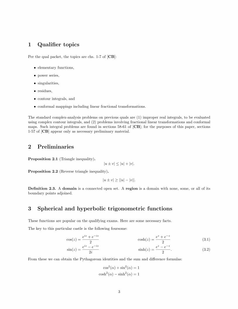
1 Qualifier topics

Per the qual packet, the topics are chs. 1-7 of [CB]:

• elementary functions,

• power series,

• singularities,

• residues,

• contour integrals, and

• conformal mappings including linear fractional transformations.

The standard complex-analysis problems on previous quals are (1) improper real integrals, to be evaluatedusing complex contour integrals, and (2) problems involving fractional linear transformations and conformalmaps. Such integral problems are found in sections 58-61 of [CB]; for the purposes of this paper, sections1-57 of [CB] appear only as necessary preliminary material.

2 Preliminaries

Proposition 2.1 (Triangle inequality).|u± v| ≤ |u|+ |v|.

Proposition 2.2 (Reverse triangle inequality).

|u± v| ≥ ||u| − |v||.

Definition 2.3. A domain is a connected open set. A region is a domain with none, some, or all of itsboundary points adjoined.

3 Spherical and hyperbolic trigonometric functions

These functions are popular on the qualifying exams. Here are some necessary facts.

The key to this particular castle is the following foursome:

cos(z) =eiz + e−iz

2cosh(z) =

ez + e−z

2(3.1)

sin(z) =eiz − e−iz

2isinh(z) =

ez − e−z

2. (3.2)

From these we can obtain the Pythagorean identities and the sum and difference formulas:

cos2(α) + sin2(α) = 1

cosh2(α)− sinh2(α) = 1

3

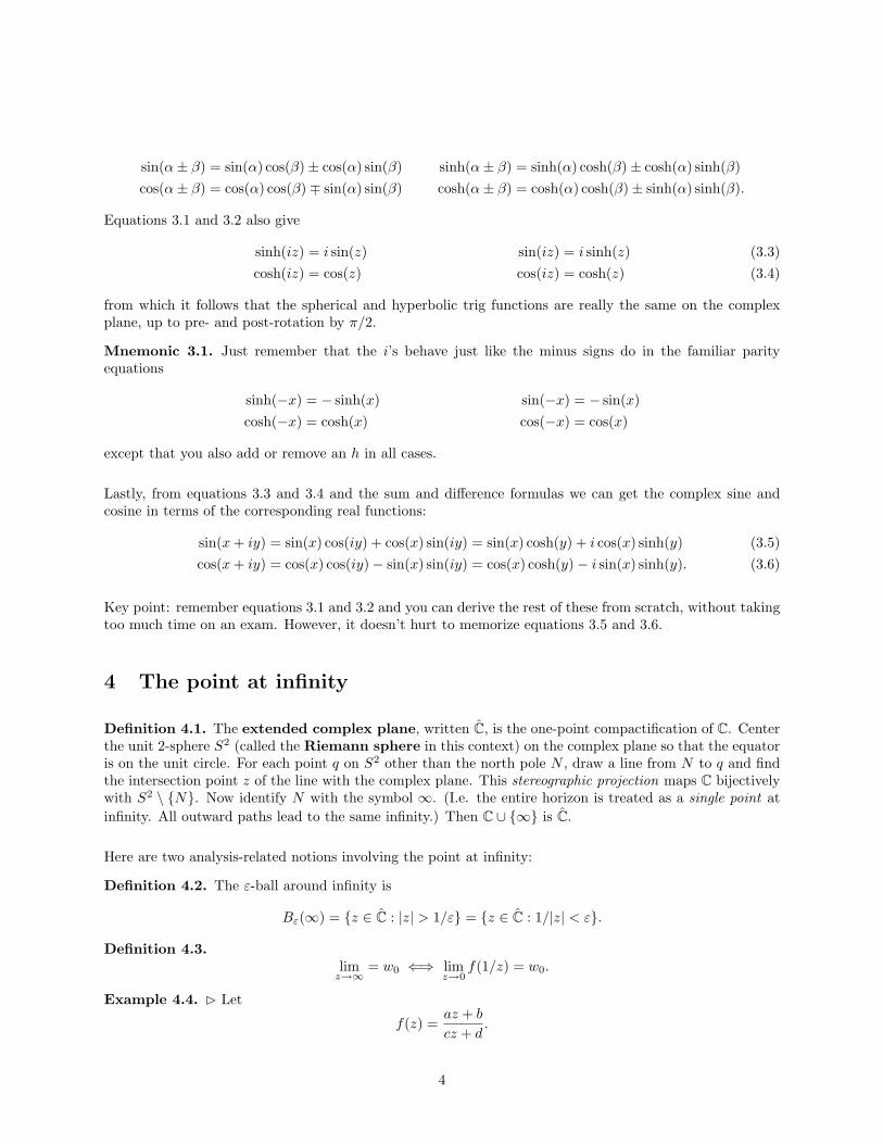
sin(α± β) = sin(α) cos(β)± cos(α) sin(β) sinh(α± β) = sinh(α) cosh(β)± cosh(α) sinh(β)cos(α± β) = cos(α) cos(β)∓ sin(α) sin(β) cosh(α± β) = cosh(α) cosh(β)± sinh(α) sinh(β).

Equations 3.1 and 3.2 also give

sinh(iz) = i sin(z) sin(iz) = i sinh(z) (3.3)cosh(iz) = cos(z) cos(iz) = cosh(z) (3.4)

from which it follows that the spherical and hyperbolic trig functions are really the same on the complexplane, up to pre- and post-rotation by π/2.

Mnemonic 3.1. Just remember that the i’s behave just like the minus signs do in the familiar parityequations

sinh(−x) = − sinh(x) sin(−x) = − sin(x)cosh(−x) = cosh(x) cos(−x) = cos(x)

except that you also add or remove an h in all cases.

Lastly, from equations 3.3 and 3.4 and the sum and difference formulas we can get the complex sine andcosine in terms of the corresponding real functions:

sin(x + iy) = sin(x) cos(iy) + cos(x) sin(iy) = sin(x) cosh(y) + i cos(x) sinh(y) (3.5)cos(x + iy) = cos(x) cos(iy)− sin(x) sin(iy) = cos(x) cosh(y)− i sin(x) sinh(y). (3.6)

Key point: remember equations 3.1 and 3.2 and you can derive the rest of these from scratch, without takingtoo much time on an exam. However, it doesn’t hurt to memorize equations 3.5 and 3.6.

4 The point at infinity

Definition 4.1. The extended complex plane, written C, is the one-point compactification of C. Centerthe unit 2-sphere S2 (called the Riemann sphere in this context) on the complex plane so that the equatoris on the unit circle. For each point q on S2 other than the north pole N , draw a line from N to q and findthe intersection point z of the line with the complex plane. This stereographic projection maps C bijectivelywith S2 \ {N}. Now identify N with the symbol ∞. (I.e. the entire horizon is treated as a single point atinfinity. All outward paths lead to the same infinity.) Then C ∪ {∞} is C.

Here are two analysis-related notions involving the point at infinity:

Definition 4.2. The ε-ball around infinity is

Bε(∞) = {z ∈ C : |z| > 1/ε} = {z ∈ C : 1/|z| < ε}.

Definition 4.3.lim

z→∞= w0 ⇐⇒ lim

z→0f(1/z) = w0.

Example 4.4. B Let

f(z) =az + b

cz + d.

4

Thenf(0) = b/d

whereas

f(∞) = limz→0

a/z + b

c/z + d

= limz→0

a + bz

c + dz= a/c.

See also section 12. C

5 Continuity, differentiability, and analyticity

Let f : C → C.

Definition 5.1. Continuity is taken in the elementary sense: f is continuous at z0 if

• limz→z0 f(z) exists, and

• f(z0) exists, and

• the two are equal.

Definition 5.2. Differentiability is taken in the elementary sense: f is differentiable at z0 if

limz→z0

f(z)− f(z0)z − z0

exists.

On the real line, there are only two ways for x to approach x0: from the left, and from the right. In thecomplex plane, there are infinitely many paths. Fortunately, we have a criterion for differentiability.

Notation 5.3. Write w = f(z) with w = u + iv and z = x + iy. Then w = u(x, y) + iv(x, y) whereu, v : R2 → R. Write ux for ∂u/∂x and likewise for uy, vx, and vy.

Proposition 5.4 (Cauchy-Riemann equations). If ux = vy and uy = −vx at z0, then f is differentiable atz0. If ux, uy, vx, and vy are continuous, then the converse is true as well.

Example 5.5. The function f(z) = z2 = (x + iy)2 is differentiable everywhere by Cauchy-Riemann; thefunction f(z) = |z|2 = x2 + y2 is differentiable only at zero. This is perhaps counterintuitive: these twofunctions are identical when restricted to the real line, where they are a nice, familiar parabola.

Definition 5.6. Note that we defined differentiability at a point. If f is differentiable on an open set U ,then f is said to be holomorphic on U . If f is holomorphic on all of C, then f is said to be entire.

Remark 5.7. Churchill and Brown say that f is analytic if it is holomorphic in the above sense. (Since Iam following Churchill and Brown, I will use the term analytic in place of holomorphic after this.) There isa technical distinction (see the Wikipedia [Wik] article on holomorphic for details):

• A (real or complex) function is said to be (real or complex) analytic if it is locally expressible as aconvergent power series, i.e. has a Taylor-series expansion at each point. This requires the function tobe infinitely differentiable (smooth).

5

• A real function can be merely differentiable without being smooth: One can devise functions whichare n times differentiable without being n + 1 times differentiable. Furthermore, a function may besmooth without being real analytic. (The standard example [Wik] is e−1/x2

with value 0 filled inat 0.) Thus, there are proper containments: continuous (C0) functions, differentiable (C1) functions,twice-differentiable (C2) functions, . . . , smooth (C∞) functions, and real analytic function.

• For complex functions, though, these classes of functions are all the same (which justifies Churchilland Brown’s use of the term analytic several chapters before defining power series): we will see intheorem 6.22 that a complex function which is once differentiable on an open set is necessarily infinitelydifferentiable on that open set, and is analytic in the power-series sense.

I believe harmonic conjugates are not needed for the qual, so I will not discuss them.

Definition 5.8. A function f is said to be singular at z0 if it is not analytic at z0 but is analytic at somepoint in every neighborhood of z0.

Definition 5.9. A function f is said to have an isolated singular point at z0 if f is singular at z0, andmoreover there is a deleted neighborhood 0 < |z − z0| < ε such that f is analytic at every point in theneighborhood.

Example 5.10. Take f(z) = 1/z. This has an isolated singular point at 0.

6 Paths and integration

Definition 6.1. Let w : [a, b] → C, with w = u + iv as above. (I suppose we can call such a general w apath, although we will use other words when w satisfies additional criteria.) Then define the integral of acomplex-valued function w(t) of a real variable to be∫ b

a

w(t)dt =∫ b

a

u(x(t), y(t))dt + i

∫ b

a

v(x(t), y(t))dt.

Likewise, w has derivativew′(t) = u′(t) + iv′(t).

Proposition 6.2. ∣∣∣∣∣∫ b

a

w(t)dt

∣∣∣∣∣ ≤∫ b

a

|w(t)|dt.

This is well and good, but we want to be able to integrate complex-valued functions f(z) of a complexvariable as well. Real integrals are defined for t on line segments; in the complex plane, we have anotherdegree of freedom of motion for z and we need to define the notion of path.

Definition 6.3. Here are some kinds of paths:

• An arc z(t) = x(t) + iy(t) is a path with x(t) and y(t) being continuous functions on t ∈ [a, b].

• A simple arc is one that does not cross itself, except perhaps at the endpoints: t1 6= t2 and t1, t2 6= a, bimplies w(t1) 6= w(t2).

• A closed curve is an arc for which w(a) = w(b).

• A smooth arc has a continuous tangent vector.

6

• A contour is a piecewise smooth arc, with finitely many pieces.

Remark 6.4. Churchill and Brown here refer to the Jordan curve theorem, which is intuitively undeniable:a simple closed curve separates C into a bounded interior and an unbounded exterior.

Intuition 6.5. Perhaps the only “definition” you need for contours is the following: all the kinds of pathswe normally think to integrate over — line segments, semicircles, etc. — are contours.

Definition 6.6. Now we can define a contour integral. This could be defined as a Riemann sum, or bymaking use of definition 6.1: ∮

C

f(z)dz =∫ b

a

f(z(t))dz

dtdt.

We immediately wonder if and when the value of the integral depends on the path taken.

Proposition 6.7. Let f be continuous on a domain D. The following are equivalent:

• f has an antiderivative F on D;

• integrals along not-necessarily-closed paths in D are independent of path;

• integrals around closed contours in D are zero.

Remark 6.8. The hypothesis is continuity, not analyticity.

Remark 6.9. This means that interesting contour integrals will need to have at least a discontinuity withinthe contour.

Theorem 6.10 (ML estimate). Let C be a contour, of arc length L. Furthermore suppose that |f(z)| ≤ Mfor all z ∈ C. Then ∣∣∣∣∫

C

f(z)dz

∣∣∣∣ ≤ ML.

Proof (David Herzog). Let z(t) be a parameterization of the contour C for t ∈ [0, 1]. Then∫C

f(z)dz =∫ 1

0

f(z(t))dz

dtdt.

Since |f(z)| ≤ M on C, ∣∣∣∣∫C

f(z)dz

∣∣∣∣ ≤∫ 1

0

|f(z(t))| |z′(t)| dt

≤ M

∫ 1

0

|z′(t)| dt

≤ ML.

Remark 6.11. This theorem is not profound, but it is crucial for qual-type calculations. See section 10.

Theorem 6.12 (Maximum modulus principle). If a function f is analytic and not constant in a givendomain D, then |f(z)| has no maximum value in D.

7

Theorem 6.13 (Jordan’s inequality). Let CR be the semicircle of radius R given by Reiθ for θ from 0 toπ. Suppose q(z) is a rational function with all its upper-half-plane zeroes below CR. If there is an MR suchthat |q(z)| ≤ MR for all z ∈ CR and such that MR → 0 as R →∞, then for all positive real a,∫

CR

q(z)eiazdz → 0 as R →∞.

Theorem 6.14 (Jordan’s lemma). Let CR be the semicircle of radius R given by Reiθ for θ from 0 to π.Suppose f(z) is a function which is analytic on all of the upper half-plane exterior to the circle |z| = R0. Ifthere is an MR such that |q(z)| ≤ MR for all z ∈ CR and such that MR → 0 as R →∞, then for all positivereal a, ∫

CR

f(z)eiazdz → 0 as R →∞.

Theorem 6.15 (Cauchy-Goursat). If f is analytic on and in a simple closed contour C, then∮C

f(z)dz = 0.

Here is an extension:

Proposition 6.16. If f is analytic throughout a simply connected domain D, then for all closed contoursC (not necessarily simple closed contours), ∮

C

f(z)dz = 0.

Corollary 6.17. If f is analytic on a simply connected domain D, then f has an antiderivative on D.

Theorem 6.18 (Cauchy integral formula). If f is analytic on and in a simple closed contour C, and if z0

is in the interior of C, then

f(z0) =1

2πi

∮C

f(z)dz

z − z0.

Remark 6.19. This differs from Cauchy-Goursat in that a discontiunity has intentionally been inserted viadividing by z − z0.

Corollary 6.20 (Gauss mean value). If f is analytic in and on the circle of radius ρ centered at z0, then

f(z0) =12π

∫ 2π

0

f(z0 + ρeiθ)dθ.

Proof. In the Cauchy integral formula, put z = z0 + ρeiθ. Then dz = ρieiθdθ. Write it down and simplify,and you’re done.

Proposition 6.21 (Deformation of paths). If C2 is inside C1, and if f is analytic in the intermediate region,then ∮

C1

f(z)dz =∮

C2

f(z)dz =∮

C

f(z)dz

for all C in that intermediate region.

Theorem 6.22. If f is analytic at a point, then it is infinitely differentiable and all its derivatives areanalytic. Specifically,

f (n)(z0) =n!2πi

∮C

f(z)dz

(z − z0)n+1.

8

In particular,

f ′(z0) =1

2πi

∮C

f(z)dz

(z − z0)2.

Sketch of proof. xxx fill in some details here. First do f ′ using continuity of f : approximate f(z) by f(z0)and use the ML estimate (6.10). Then, use induction for higher derivatives.

Remark 6.23. This generalizes the Cauchy integral formula (theorem 6.18).

Theorem 6.24 (Morera). (Converse to Cauchy-Goursat if D is simply connected.) If f is continuous on adomain D and if

∮C

f(z)dz = 0 for all closed contours C contained in D, then f is analytic on D.

Theorem 6.25 (Liouville). If f is bounded on all of C and if f is entire, then f is constant.

7 Power series

Theorem 7.1 (Taylor series). Let f be analytic in the open disk

D = {z ∈ C : |z − z0| < R}.

Then for all z ∈ D, f has the power series representation

f(z) =∞∑

n=0

f (n)(z0)(z − z0)n

n!

Remark 7.2. If f is entire then the radius R may be taken arbitrarily large.

Remark 7.3. Recall from theorem 6.22 that for analytic f we also have

f (n)(z0) =n!2πi

∮C

f(s)ds

(s− z0)n+1.

Combining these two facts, we have

f(z) =∞∑

n=0

(1

2πi

∮C

f(s)ds

(s− z0)n+1

)(z − z0)n.

Mnemonic 7.4. If we “cancel” powers of (z − z0) outside the sum with powers of (s− z0) inside the sum,then we get the same exponent as in the Cauchy integral formula (theorem 6.18).

Note that in order to use a Taylor expansion, we need f to be analytic on an open disk. What if we have afunction that is somehow singular, e.g. if f itself is analytic but we consider f(z)/(z − z0)?

Theorem 7.5 (Laurent series). Let f be analytic in the annulus

A = {z ∈ C : R < |z − z0| < S}.

Then for all z ∈ A, f has the power series representation

f(z) =∞∑

n=−∞

(1

2πi

∮C

f(s)ds

(s− z0)n+1

)(z − z0)n.

9

Remark 7.6. If f is analytic in the disk (i.e. in the filled annulus) then one would expect the Laurent seriesto reduce to a Taylor series. Indeed this is the case: for analytic f and negative n,

f(z)(z − z0)n+1

= f(z)(z − z0)−n−1

is the product of two analytic functions, hence analytic, so by Cauchy-Goursat the coefficients for negativen are indeed zero.

Once we have a power series, we immediately want to be able to integrate and differentiate term by term.For the former, we have a stronger result. First, though, we need a definition.

Definition 7.7. Every power series

S(z) =∞∑

n=0

an(z − z0)n

has a (perhaps infinite, perhaps zero-radius) circle of convergence centered at z0:

• S is (absolutely) convergent for all z interior to S.

• S is divergent for all z exterior to S.

Proposition 7.8. Let

S(z) =∞∑

n=0

an(z − z0)n

be a power series. Let C be a contour interior to the circle of convergence of S. Let g(z) be any functionthat is continuous on C. Then g(z)S(z) may be integrated term by term along C. That is,∫

C

g(z)

( ∞∑n=0

an(z − z0)n

)dz =

∞∑n=0

an

∫C

g(z)(z − z0)ndz.

Proposition 7.9. Let

S(z) =∞∑

n=0

an(z − z0)n

be a power series. Then S may be differentiated term by term, i.e.

S′(z) =∞∑

n=1

nan(z − z0)n−1,

anywhere inside its circle of convergence.

8 Zeroes and poles

Definition 8.1. Let f be analytic in an annulus A centered at z0. Then f has Laurent series expansion forz ∈ A.

• The principal part of f is the series with only negative-n coefficients included.

• Let m be index of the lowest-index non-zero coefficient in the Laurent series, if any.

10

• If there is no such m, then f is said to have an essential singularity at z0. (For example, write outthe Taylor series for ez about z0 = 0, then replace z’s with 1/z’s to get a Taylor series for e1/z.)

• If m is negative, f is said to have a pole of order −m at z0. (For example, f(z) = 1/z3 at z0 = 0.)

• If m is positive, f is said to have a zero of order m at z0. (For example, f(z) = z3 at z0 = 0.)

• A pole of order 1 is called a simple pole.

• A zero of order 1 is called a simple zero.

• If m exists and is non-negative but f is singular at z0 (see definition 5.8), then f is said to have aremovable singularity at z0. (For example, take sin(z)/z. Write out the Taylor series for sin(z),then divide through by z: you will see no z’s in any denominator.)

Definition 8.2. A complex-valued function is said to be meromorphic or regular on an open subset Uof C if it is holomorphic on all of U except for a set of isolated poles.

Remark 8.3. A meromorphic function may be written as the ratio of holomorphic functions, with denomi-nator not identically zero. The canonical example is rational functions. Since polynomials are entire, rationalfunctions are meromorphic on all of C.

Mnemonic 8.4. Silly but memorable: mero is ratio of holo.

9 Residues

If f has an isolated singular point z0 (definition 5.9), then it is analytic in some deleted open neighborhoodof D z0. Thus it has a Laurent-series expansion about z0.

Definition 9.1. Let∞∑

n=−∞ak(z − z0)n

be the Laurent series expansion of f on D. The residue of f at z0 is the coefficient on 1/(z − z0) in theLaurent series expansion of f :

Resz=z0

f(z) = a−1.

By theorem 7.5 we see that this is the same as

Resz=z0

f(z) =1

2πi

∮C

f(z)dz

for a positively oriented simple closed contour C lying in D. By Cauchy-Goursat (theorem 6.15), if f isanalytic at z0 it has zero residue there.

For poles (i.e. non-essential singularities), we have the following alternative formulas.

Proposition 9.2. If f(z) can be written as

f(z) =φ(z)

z − z0

with φ analytic and non-zero at z0 (e.g. if f has a zero of order 1 at z0) then

Resz=z0

f(z) = φ(z0).

11

If f(z) can be written as

f(z) =φ(z)

(z − z0)m

with φ analytic and non-zero at z0 (e.g. if f has a zero of order m at z0) then

Resz=z0

f(z) =φ(m−1)(z0)(m− 1)!

.

If f(z) can be written as

f(z) =g(z)h(z)

where g is analytic at z0 and h has a simple zero at z0, then

Resz=z0

f(z) =g(z0)h′(z0)

.

Example 9.3. B The choice of formula can be significant, when one is pressed for time. Let

f(z) =z1/2

z3 + 1,

taking the principal branch of the square root, and suppose we want to compute the sum of residues overpoles of f(z). Note that the denominator has the three roots [xxx include figure here]

z1 = −1z2 = ζ6 = eiπ/3 = 1/2 + i

√3/2

z3 = ζ6 = e−iπ/3 = 1/2− i√

3/2.

Using the first formula, we have

Resz=z1

f(z) =z1/21

(z1 − z2)(z1 − z3)

Resz=z2

f(z) =z1/22

(z2 − z1)(z2 − z3)

Resz=z3

f(z) =z1/23

(z3 − z1)(z3 − z2).

You can get out your calculator and find that these are (respectively)

i/3, −i/3, i/3.

Doing it by hand, though, gives several opportunities for arithmetic errors.

Using the second formula, with g(z) = z1/2 and h(z) = z3 + 1, so h′(z) = 3z2, we have

Resz=z1

f(z) =z1/21

3z21

=1

3z3/21

Resz=z2

f(z) =z1/22

3z22

=1

3z3/22

Resz=z3

f(z) =z1/23

3z23

=1

3z3/23

.

12

There’s no subtraction going on, and trivial division, so the computation is less error-prone. The only catchis keeping track of the branches of the square root function. [xxx figure here.]

z3/21 = i

z3/22 = −i

z3/23 = i

so the sum of residues isi/3− i/3 + i/3 = i/3.

C

Theorem 9.4 (Residue theorem). Let C be a positively oriented simple closed contour. If f is analytic onand in C except at a finite number of singular points zk for k = 1, 2, . . . , n interior to C, then

12πi

∮C

f(z)dz =n∑

k=1

Resz=zk

f(z).

Theorem 9.5 (Cauchy’s argument principle). Let C be a simple closed curve. Let f(z) be a function whichis meromorphic in and on C, with no zeroes or poles on the boundary C. Let N and P be the number ofzeroes and poles, respectively, of f interior to C, counted with multiplicity. Then∮

C

f ′(z)f(z)

dz = 2πi(N − P ).

10 Integration

Now we come to the reason for everything up to this point: to use residues and contours to evaluate certainimproper real integrals. We use the residue theorem (theorem 9.4) and the residue formulas in proposition9.2. The canonical example is show that

∫ +∞−∞

sin(x)x dx = π.

First a definition which often arises in real integrals. What do we mean by∫ +∞−∞ f(x)dx — precisely how do

the left and right endpoints go to their respective infinities?

Definition 10.1. The Cauchy principal value of the improper integral∫ +∞

−∞f(x)dx,

written with a dash through the integral sign (for which I lack a pre-made LATEX symbol), is

lima→∞

∫ a

a

f(x)dx.

The need for this definition is best illustrated by example.

Example 10.2. B Let f(x) = x. One might think that∫ +∞−∞ f(x)dx should be zero — after all, doesn’t

the negative area on the left cancel the positive area on the right? Well, it does if you let the left and rightedges go to zero at precisely the same rate. But this setup is fragile — you get something non-zero if youtweak it in some reasonable ways. First,

lima→∞

∫ 2a

a

f(x)dx

13

looks graphically like it shoots off to +∞. Likewise,

lima→∞

∫ a

2a

f(x)dx

looks like −∞. The other tweak is translation invariance. Namely,∫ +∞

−∞f(x)dx

ought to be the same as ∫ +∞

−∞f(x + c)dx.

Shift f(x) = x by a constant and you’ll see that the Cauchy principal value isn’t zero.

My point here is that absolute integrability (which f(x) = x lacks) is a necessary condition for a well-definedintegral — one which is translation invariant and independent of parameterization of endpoints. The Cauchyprincipal value is best thought of as a consolation prize when a true integral is not possible. C

Remark 10.3. If the integrand f(x) is even, then∫ +∞

−∞f(x)dx = 2

∫ +∞

0

f(x)dx.

rat’l fcns, sin/cos times rat’l, sin/cos definite int’l, thru branch cut

Use z1/2/(1 + z3) as an example:

• Two different ways to compute residues (one better).

• Keyhole path. C1 is the desired; C2 is circle with R →∞; C3 appears to be negative of desired but isnot due to the square-root branch; C4 is circle the other way with r → 0.

C3: ∫ R

r

x1/2

x3 + 1dx

but here [xxx figure] x1/2 = −x rather than −√

x. So∫ r

R

−√

x

x3 + 1dx =

∫ R

r

−√

x

x3 + 1dx.

• Define the branch of the square root: Reiθ 7→√

Reiθ/2 for 0 ≤ θ < 2π.

• Note easy numerical check for the integral. Also graph the integrand.

• How to estimate integral on inner and outer circles? For small z, f(z) ≈ z1/2/1 → 0; for large z,f(z) ≈ z1/2/z3 → 0. Then couple that with an ML estimate.

14

11 Conformal maps

Definition 11.1. A function f : C → C is conformal at a point z0 if it is analytic at z0 and f ′(z0) 6= 0.Likewise, it is conformal on a domain D if it is analytic at each point of D.

Proposition 11.2. Conformal maps are angle-preserving.

Proof. (This discussion is adapted from [CB].) Let z1(t), z2(t) be curves intersecting at a common point z0

at time t0, i.e. z1(t0) = z2(t0) = z0. Let w1(t) = f(z1(t)) and w2(t) = f(z2(t)). The key insight is that theangle between curves is (up to 2π) the difference of the complex phases of their derivatives. [xxx includefigure here.] Using the chain rule, we have

w′1(t) = f ′(z1(t))z′1(t) and w′2(t) = f ′(z2(t))z′2(t).

When we multiply two complex numbers , their phases add. So,

Arg(w′1(t)) = Arg(f ′(z1(t))) + Arg(z′1(t))Arg(w′2(t)) = Arg(f ′(z2(t))) + Arg(z′2(t)).

But the two curves intersect at t0, so when t = t0, the first terms after the equals signs are the same.Subtracting, we have

Arg(w′1(t0))−Arg(w′2(t0)) = Arg(z′1(t))−Arg(z′2(t)).

That is, the difference in phases of the image curves is the same as the difference in phases of the originalcurves, which is what we mean by angle-preserving.

Example 11.3. B Let z1(t) = t and z2(t) = it, with t0 = 0. Let f(z) = ez. Then

f ′(zi(t0)) = f ′(0) = e0 = 1

z′1(t0) = 1 z′2(t) = i

w1(t) = et w2(t) = eit

w′1(t) = et w′2(t) = ieit

sow′1(0) = 1 and w′2(t) = i.

The input phases are 0 and π/2 respectively, as are (in this trivial example) the output phases. C

Proposition 11.4. Conformal maps preserve fundamental groups.

Theorem 11.5 (Riemann mapping theorem). Let U be a simply connected open subset of C, which is notall of C. Then there exists a bijective holomorphism f : U → {z ∈ C : |z| < 1}.

Remark 11.6. This means f is conformal as well. [xxx talk about f ′(z) 6= 0.]

An important topic on qualifying exams is the construction of a conformal map sending one region to another,say, the upper half-plane to the unit disk. The key to success here is the big five:

• z 7→ ez

• z 7→ sin(z)

15

• z 7→ 1/z.

• z 7→ z + 1/z

• z 7→ z−iz+i

Also there are the more obvious little three:

• z 7→ iz

• z 7→ z + c

• Composition.

Of course, a qualifying-exam author may devise something nefarious, unaddressable by items on this list.However, one hopes that some ad-hoc reasoning of the form given below might suffice to get a person throughthe morning.

It turns out to be most important to tabulate what each of these does to

• the upper half-plane,

• the unit disk,

• horizontal strips, and

• vertical strips.

As much as I’d love to doodle up some nice figures (and someday I may), you can find these in any complex-analysis text, Mathworld, etc. My added value here is to focus on which conformal maps come up most oftenon the quals. Here are some useful facts (letting z = x + iy throughout):

• ez takes the horizontal strip 0 ≤ y ≤ π to the upper half-plane. To remember this, write out ez =ex+iy = exeiy. Then think about what happens when x or y is held fixed. For each x, we have asemicircle in the upper half-plane with radius ex.

• ez takes the half-horizontal strip 0 ≤ y ≤ π and x > 0 to the upper half-plane, minus the unit disk.Since x > 0, the radii of the circles are ex > 1.

• ez takes the half-horizontal strip 0 ≤ y ≤ π and x ≤ 0 to the half of the unit disk in the upperhalf-plane: Since x ≤ 0, the radii of the circles are ex > 1.

• ez takes the vertical strip 0 ≤ x ≤ 1 to the annulus with inner radius 1 and outer radius e: For eachx from 0 to 1, ex ranges from 1 to e and so exeiy traces out circles as y runs along. Similarly, we canfind the image of a rectangle under ez.

• sin z takes vertical lines to ellipses and horizontal lines to hyperbols. (Be sure to find a picture of thismap — it’s very pretty.) To remember this, recall that

sin(x + iy) = sin x cosh y + i cos x sinh y.

The images of horizontal line segments are the upper halves of ellipses with horizontal radius cosh yand vertical radius sinh y; the images of vertical lines are hyperbolas. (See my geometry-topology qualsolutions, Fall 2004 #2, for a derivation of the formula, and further discussion of this map.)

16

• 1/z sends the unit circle to itself, and sends the interior of the unit circle to its exterior and vice versa.

• 1/z sends the circle centered at 1 (so the left edge is at x = 0 and the right edge is at x = 2) to thehalf-plane x ≥ 1/2. And vice versa of course, since 1/(1/z) = 1.

• 1/z . . . .

• 1/z . . . .

• 1/z . . . .

• z + 1/z sends . . . . Note CB p. 27: u = (r + 1/r) cos θ; v = (r − 1/r) sin θ (ellipse!). Spell these outand from that derive a mnemonic for the image of the upper and lower half-disks.

• (z − 1)/(z + 1) sends . . . . Also mention (z − i)/(z + i) in terms of pre-rotation. Also xref forward toLFTs.

Example 11.7. B Let z = x + iy. Find a conformal map sending the horizontal strip 0 ≤ y ≤ 1 to the unitdisk.

Reading off the above information, we see ez sending the horizontal strip 0 ≤ y ≤ π to the upper half-plane,and (z − 1)/(z + 1) sending the right half-plane to the unit disk. So, compose:

• Map the horizontal strip 0 ≤ y ≤ 1 to the horizontal strip 0 ≤ y ≤ π by multiplication by π.

• Send that to the right half-plane by ez.

• Rotate that to the upper half-plane by multiplying by i.

• Send that to the unit disk by (z − 1)/(z + 1).

Let’s write out the compositions one step at a time. (I know I’ll make an algebra mistake if I try to write itall out at once.)

w1 = πz

w2 = eπz

w3 = ieπz

w4 =ieπz − 1ieπz + 1

.

C

xxx double-check this.

xxx do it using 1/z.

12 Linear fractional transformations

(This section is due mostly to Victor Piercey.)

Definition 12.1. A linear fractional transformation (also known as a Mobius transformation) is amap T : C → C given by

T (z) =az + b

cz + d

where a, b, c, d ∈ C with ad− bc 6= 0.

17

Definition 12.2. I call the quantity ad− bc, for lack of a better name, the determinant of T .

Next, several facts.

Proposition 12.3. LFTs are invertible via

T−1(z) =−dz + b

cz − a.

Proof. Compose both directions and simplify, obtaining the identity each time.

Proposition 12.4. The composition of LFTs is another LFT.

Proof. Write out the composition of

z 7→ az + b

cz + dand z 7→ ez + f

gz + h.

The determinant (after some algebra) factors as

(ad− bc)(eh− fg),

i.e. the product of determinants of the two original LFTs, which is non-zero iff both the original determinantsare non-zero.

Since the identity is an LFT and composition is associative, we have shown:

Proposition 12.5. The set of all LFTs is a group with respect to composition.

Remark 12.6. LFTs extend to C with

T (∞) = a/c and T (−d/c) = ∞.

(Recall that a/c = ∞ if c = 0: see example 4.4.) From here on out, we will consider our LFTs to be on C.

Remark 12.7. The group of all LFTs is sometimes called Aut(C), isomorphic to PGL2(C); it is the auto-morphism group of the Riemann sphere. (See the very nice Wikipedia article on Linear Fractional Transfor-mations.) I’m not aware of any (as-yet-written) qual problems which make use of this fact, but keep an eyeout for covering-space questions.

Lemma 12.8. Every LFT other than the identity has at most two fixed points.

Proof. Suppose we have a fixed point, namely,

z = T (z) =az + b

cz + d.

Clearing denominators givescz2 + (d− a)z − b = 0.

• If c 6= 0, this is a quadratic with complex coefficients, so either there are two distinct roots, or there isone repeated root.

• If c = 0 and d 6= a then it is linear, with one root; it fixes 0 and ∞.

18

• If c = 0 and d = a and b 6= 0 then it has no roots. However T does fix ∞.

• If c = 0 and d = a and b = 0 then it has infinitely many roots, but then one of the following is true:either d = a = 0, in which case a = b = c = d = 0 and T is not an LFT, or a, d 6= 0 and T is theidentity transformation.

This definition is used in the proof of the following lemma.

Definition 12.9. Given three distinct complex numbers z1, z2, and z3, let A(z) be the LFT given by

A(z) =(

z − z1

z − z3

)(z2 − z3

z2 − z1

).

This is called the implicit form for A.

Proposition 12.10. These are, in fact, LFTs.

Proof. Distributing the top and bottom, we get(z − z1

z − z3

)(z2 − z3

z2 − z1

)=

(z2 − z3)z − (z2 − z3)z1

(z2 − z1)z − (z2 − z1)z3.

This has determinant equal to(z2 − z3)(z2 − z1)(z3 − z1).

This is non-zero iff z1, z2, and z3 are distinct.

The next result is of key importance for qualifying exams.

Proposition 12.11. A linear fractional transformation is uniquely specified by its action on three distinctpoints.

Proof, from Fisher’s text. Let the three distinct points be z1, z2, and z3, with images w1 = T (z1), w2 =T (z2), and w3 = T (z3). Define one LFT, A, such that

A(z1) = 0, A(z2) = 1, and A(z3) = ∞;

define another LFT, B, such that

B(w1) = 0, B(w2) = 1, and B(w3) = ∞.

The existence of A and B is guaranteed by the existence of their implicit forms. Then

B−1Azi = wi

for i = 1, 2, 3, soT−1B−1Azi = zi.

for i = 1, 2, 3. This is a composition of LFTs, hence an LFT, with three fixed points. By the lemma, it isthe identity transformation, i.e. T = B−1A.

The following facts aid in the construction of LFTs.

19

Proposition 12.12. LFTs map circles and lines to circles or lines.

Remark 12.13. LFTs are compositions of

z 7→ az, z 7→ z + b, and z 7→ 1/z.

Technique 12.14 (Churchill and Brown). To write down an LFT given three points z1, z2, and z3, andtheir images w1, w2, and w3, as long as none of these points is at infinity, write down(

w − w1

w − w3

)(w2 − w3

w2 − w1

)=(

z − z1

z − z3

)(z2 − z3

z2 − z1

)and solve for z. If any zi or wi is ∞, replace it with 1/zi or 1/wi, respectively, then set it to zero aftersimplifying.

Example 12.15. B Find an LFT sending 0 to 1, 1 to ∞, and ∞ to 0.

We have

z1 = 0 w1 = 1z2 = 1 w2 = ∞z3 = ∞ w3 = 0.

Then we need to solve for w:(w − 1

w

)(1/w2

1/w2 − 1

)=

(z

z − 1/z3

)(1− 1/z3

1

)(

w − 1w

)(1

1− w2

)=

(z

z3z − 1

)(z3 − 1

1

)(

w − 1w

)= z

w − 1 = zw

w − zw = 1

w =1

1− z.

Now check, using definition 4.3:

11− 0

= 1

11− 1

= ∞

11−∞

= limz→0

11− 1/z

= limz→0

z

z − 1= 0

as desired. C

Alternatively, one can plug in each of the three inputs and solve the resulting system of equations.

20

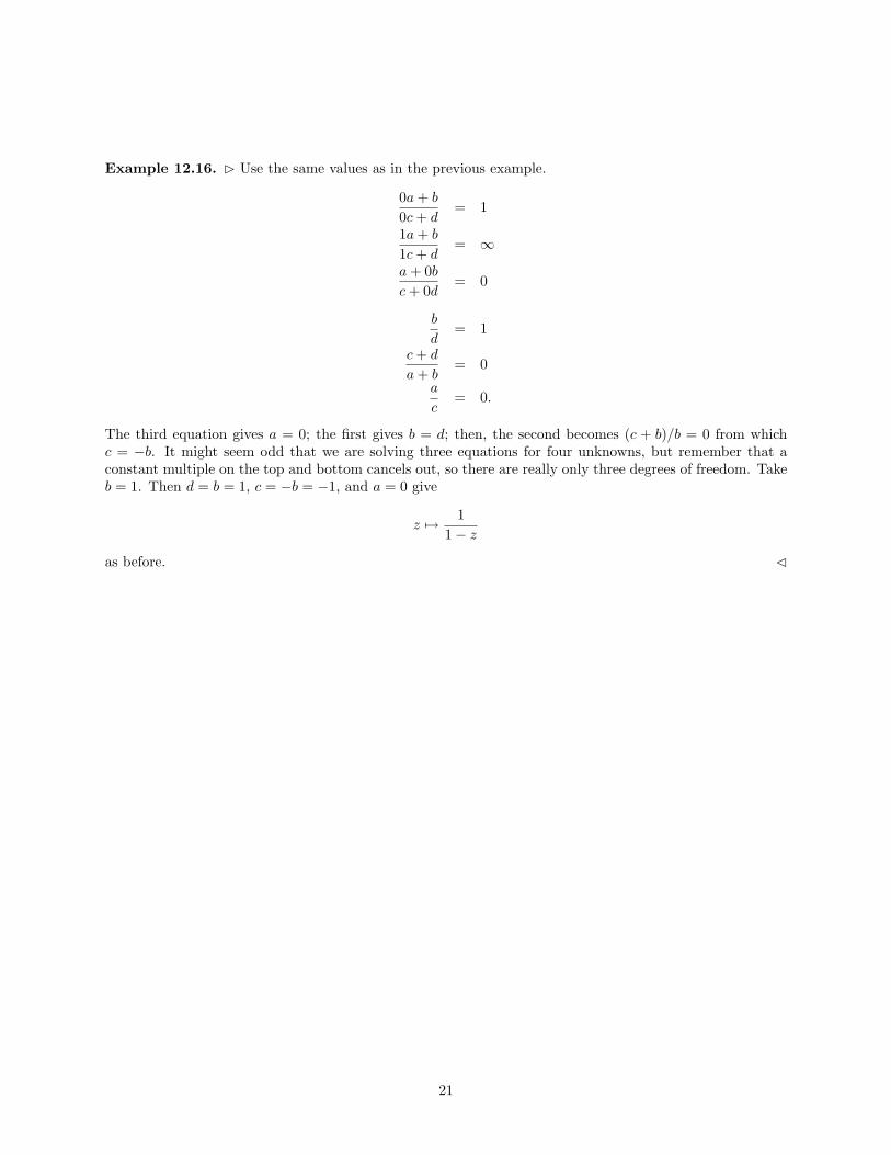
Example 12.16. B Use the same values as in the previous example.

0a + b

0c + d= 1

1a + b

1c + d= ∞

a + 0b

c + 0d= 0

b

d= 1

c + d

a + b= 0

a

c= 0.

The third equation gives a = 0; the first gives b = d; then, the second becomes (c + b)/b = 0 from whichc = −b. It might seem odd that we are solving three equations for four unknowns, but remember that aconstant multiple on the top and bottom cancels out, so there are really only three degrees of freedom. Takeb = 1. Then d = b = 1, c = −b = −1, and a = 0 give

z 7→ 11− z

as before. C

21

References

[CB] Churchill, R.V. and Brown, J.W. Complex Variables and Applications (5th ed.). McGraw-Hill, 1990.

[Wik] Articles on holomorphic and non-analytic smooth function. http://en.wikipedia.org.

22

23

Index

Aanalytic . . . . . . . . . . . . . . . . . . . . . . . . . . . . . . . . . . . . . . . . . . 5arc . . . . . . . . . . . . . . . . . . . . . . . . . . . . . . . . . . . . . . . . . . . . . . . 6argument principle . . . . . . . . . . . . . . . . . . . . . . . . . . . . . . 13

Bbig five . . . . . . . . . . . . . . . . . . . . . . . . . . . . . . . . . . . . . . . . . .15

CCauchy integral theorem . . . . . . . . . . . . . . . . . . . . . . . . . 8Cauchy principal value . . . . . . . . . . . . . . . . . . . . . . . . . . 13Cauchy’s argument principle . . . . . . . . . . . . . . . . . . . . 13Cauchy-Goursat theorem . . . . . . . . . . . . . . . . . . . . . . . . . 8Cauchy-Riemann equations . . . . . . . . . . . . . . . . . . . . . . .5circle of convergence . . . . . . . . . . . . . . . . . . . . . . . . . . . . 10closed curve . . . . . . . . . . . . . . . . . . . . . . . . . . . . . . . . . . . . . . 6conformal . . . . . . . . . . . . . . . . . . . . . . . . . . . . . . . . . . . . . . . 15continuous . . . . . . . . . . . . . . . . . . . . . . . . . . . . . . . . . . . . . . . 5contour . . . . . . . . . . . . . . . . . . . . . . . . . . . . . . . . . . . . . . . . . . 7

Ddeformation of paths . . . . . . . . . . . . . . . . . . . . . . . . . . . . . 8determinant . . . . . . . . . . . . . . . . . . . . . . . . . . . . . . . . . . . . .18differentiable . . . . . . . . . . . . . . . . . . . . . . . . . . . . . . . . . . . . . 5domain . . . . . . . . . . . . . . . . . . . . . . . . . . . . . . . . . . . . . . . . . . .3

Eentire . . . . . . . . . . . . . . . . . . . . . . . . . . . . . . . . . . . . . . . . . . . . 5essential singularity . . . . . . . . . . . . . . . . . . . . . . . . . . . . . 11extended complex plane . . . . . . . . . . . . . . . . . . . . . . . . . . 4

Ffundamental group . . . . . . . . . . . . . . . . . . . . . . . . . . . . . . 15

GGauss mean value theorem . . . . . . . . . . . . . . . . . . . . . . . 8

Hharmonic conjugates . . . . . . . . . . . . . . . . . . . . . . . . . . . . . 6holomorphic . . . . . . . . . . . . . . . . . . . . . . . . . . . . . . . . . . . . . .5

Iimplicit form . . . . . . . . . . . . . . . . . . . . . . . . . . . . . . . . . . . . 19improper real integrals . . . . . . . . . . . . . . . . . . . . . . . . . . 13infinity . . . . . . . . . . . . . . . . . . . . . . . . . . . . . . . . . . . . . . . . . . . 4isolated singular point . . . . . . . . . . . . . . . . . . . . . . . . . . . . 6

JJordan curve theorem . . . . . . . . . . . . . . . . . . . . . . . . . . . . 7Jordan’s inequality . . . . . . . . . . . . . . . . . . . . . . . . . . . . . . . 8

Jordan’s lemma . . . . . . . . . . . . . . . . . . . . . . . . . . . . . . . . . . 8

Llinear fractional transformation . . . . . . . . . . . . . . . . . 17Liouville’s theorem . . . . . . . . . . . . . . . . . . . . . . . . . . . . . . . 9little three . . . . . . . . . . . . . . . . . . . . . . . . . . . . . . . . . . . . . . 16

MMobius transformation . . . . . . . . . . . . . . . . . . . . . . . . . . 17maximum modulus principle . . . . . . . . . . . . . . . . . . . . . 7mean value theorem . . . . . . . . . . . . . . . . . . . . . . . . . . . . . . 8meromorphic . . . . . . . . . . . . . . . . . . . . . . . . . . . . . . . . . . . . 11ML estimate . . . . . . . . . . . . . . . . . . . . . . . . . . . . . . . . . . . . . 7Morera’s theorem . . . . . . . . . . . . . . . . . . . . . . . . . . . . . . . . 9

Oorder . . . . . . . . . . . . . . . . . . . . . . . . . . . . . . . . . . . . . . . . . . . .11

Ppath . . . . . . . . . . . . . . . . . . . . . . . . . . . . . . . . . . . . . . . . . . . . . 6path independence . . . . . . . . . . . . . . . . . . . . . . . . . . . . . . . 7point at infinity . . . . . . . . . . . . . . . . . . . . . . . . . . . . . . . . . . 4pole . . . . . . . . . . . . . . . . . . . . . . . . . . . . . . . . . . . . . . . . . . . . .11principal part . . . . . . . . . . . . . . . . . . . . . . . . . . . . . . . . . . . 10principal value . . . . . . . . . . . . . . . . . . . . . . . . . . . . . . . . . . 13

Rregion . . . . . . . . . . . . . . . . . . . . . . . . . . . . . . . . . . . . . . . . . . . . 3regular . . . . . . . . . . . . . . . . . . . . . . . . . . . . . . . . . . . . . . . . . . 11removable singularity . . . . . . . . . . . . . . . . . . . . . . . . . . . 11residue . . . . . . . . . . . . . . . . . . . . . . . . . . . . . . . . . . . . . . . . . . 11residue theorem . . . . . . . . . . . . . . . . . . . . . . . . . . . . . . . . . 13reverse triangle inequality . . . . . . . . . . . . . . . . . . . . . . . . 3Riemann mapping theorem . . . . . . . . . . . . . . . . . . . . . .15Riemann sphere . . . . . . . . . . . . . . . . . . . . . . . . . . . . . . . . . . 4

Ssimple . . . . . . . . . . . . . . . . . . . . . . . . . . . . . . . . . . . . . . . . . . . .6simple pole . . . . . . . . . . . . . . . . . . . . . . . . . . . . . . . . . . . . . .11simple zero . . . . . . . . . . . . . . . . . . . . . . . . . . . . . . . . . . . . . .11singular . . . . . . . . . . . . . . . . . . . . . . . . . . . . . . . . . . . . . . . . . . 6smooth arc . . . . . . . . . . . . . . . . . . . . . . . . . . . . . . . . . . . . . . . 6stereographic projection . . . . . . . . . . . . . . . . . . . . . . . . . . 4

Ttranslation invariance . . . . . . . . . . . . . . . . . . . . . . . . . . . 14triangle inequality . . . . . . . . . . . . . . . . . . . . . . . . . . . . . . . . 3

Zzero . . . . . . . . . . . . . . . . . . . . . . . . . . . . . . . . . . . . . . . . . . . . . 11

24