lecture notes complex analysis 7th edition brown and ...lecture notes complex analysis based on...
TRANSCRIPT

Lecture Notes
Complex Analysis
based on
Complex Variables and Applications
7th Edition
Brown and Churchhill
Yvette Fajardo-Lim, Ph.D.Department of Mathematics
De La Salle University - Manila

2

Contents
1 THE COMPLEX NUMBER FIELD 51.1 Sum and Products . . . . . . . . . . . . . . . . . . . . . . . . . . . . . . . 51.2 Basic Algebraic Properties . . . . . . . . . . . . . . . . . . . . . . . . . . . 61.3 Conjugate and Absolute Value of a Complex Number . . . . . . . . . . . 71.4 Polar and Exponential Form . . . . . . . . . . . . . . . . . . . . . . . . . . 111.5 Roots of Complex Numbers . . . . . . . . . . . . . . . . . . . . . . . . . . 141.6 Regions in the Complex Plane . . . . . . . . . . . . . . . . . . . . . . . . . 20
2 ANALYTIC FUNCTIONS 232.1 Functions of a Complex Variable . . . . . . . . . . . . . . . . . . . . . . . 232.2 Limits . . . . . . . . . . . . . . . . . . . . . . . . . . . . . . . . . . . . . . 262.3 Limits Involving the Point at Infinity . . . . . . . . . . . . . . . . . . . . . 302.4 Continuity . . . . . . . . . . . . . . . . . . . . . . . . . . . . . . . . . . . . 322.5 Derivatives . . . . . . . . . . . . . . . . . . . . . . . . . . . . . . . . . . . 342.6 Differentiation Formulas . . . . . . . . . . . . . . . . . . . . . . . . . . . . 372.7 Cauchy-Riemann Equations . . . . . . . . . . . . . . . . . . . . . . . . . . 392.8 Sufficient Conditions for Differentiability . . . . . . . . . . . . . . . . . . . 412.9 Polar Form of Cauchy-Riemann Equations . . . . . . . . . . . . . . . . . . 432.10 Analytic Functions . . . . . . . . . . . . . . . . . . . . . . . . . . . . . . . 442.11 Harmonic Functions . . . . . . . . . . . . . . . . . . . . . . . . . . . . . . 47
3 ELEMENTARY FUNCTIONS 513.1 The Complex Exponential Function . . . . . . . . . . . . . . . . . . . . . 513.2 Complex Trigonometric Functions . . . . . . . . . . . . . . . . . . . . . . 523.3 Complex Hyperbolic Functions . . . . . . . . . . . . . . . . . . . . . . . . 543.4 Complex Logarithmic Functions . . . . . . . . . . . . . . . . . . . . . . . . 563.5 Complex Inverse Trigonometric Functions . . . . . . . . . . . . . . . . . . 59
4 INTEGRALS 614.1 Definite Integrals of w(t) . . . . . . . . . . . . . . . . . . . . . . . . . . . . 614.2 Arcs and Contours . . . . . . . . . . . . . . . . . . . . . . . . . . . . . . . 634.3 Contour Integrals . . . . . . . . . . . . . . . . . . . . . . . . . . . . . . . . 674.4 Antiderivatives . . . . . . . . . . . . . . . . . . . . . . . . . . . . . . . . . 714.5 Cauchy-Goursat Theorem . . . . . . . . . . . . . . . . . . . . . . . . . . . 77
3

4 CONTENTS
4.6 Cauchy Integral Formula . . . . . . . . . . . . . . . . . . . . . . . . . . . . 894.7 Derivatives of Analytic Functions . . . . . . . . . . . . . . . . . . . . . . . 914.8 Liouville’s Theorem and the Fundamental Theorem of Algebra . . . . . . 92
5 SERIES 955.1 Convergence Of Sequences . . . . . . . . . . . . . . . . . . . . . . . . . . . 955.2 Taylor Series . . . . . . . . . . . . . . . . . . . . . . . . . . . . . . . . . . 1005.3 Laurent Series . . . . . . . . . . . . . . . . . . . . . . . . . . . . . . . . . . 107
6 RESIDUES AND POLES 1156.1 Residues . . . . . . . . . . . . . . . . . . . . . . . . . . . . . . . . . . . . . 1156.2 Cauchy’s Residue Theorem . . . . . . . . . . . . . . . . . . . . . . . . . . 1196.3 Three Types of Isolated Singular Points . . . . . . . . . . . . . . . . . . . 1226.4 Residues at Poles . . . . . . . . . . . . . . . . . . . . . . . . . . . . . . . . 1246.5 Evaluation of Improper Integrals . . . . . . . . . . . . . . . . . . . . . . . 128

Chapter 1
THE COMPLEX NUMBERFIELD
1.1 Sum and Products
Definition 1.1. A complex number, denoted by z is an ordered pair of real numbers,z = (x, y). The real number x is called the real part and the real number y is called theimaginary part of the complex number. We may write this as: x = Re z and y = Im z.
The ordered pairs (x, y) are points on the complex plane, denoted by C. The pointson this plane with coordinates (x, 0) are points on the x-axis of C and the points of theform (0, y) are points on the y-axis of C. These axes are called the real axis and theimaginary axis respectively.
Definition 1.2. Two complex numbers z1 = (x1, y1) and z2 = (x2, y2) are equal, thatis, z1 = z2 if and only if x1 = x2 and y1 = y2.
Thus, the statement zl = z2 means that zl and z2 correspond to the same point inthe complex plane.
Definition 1.3. The sum zl + z2 and the product zlz2 of two complex numbers zl =(xl, yl) and z2 = (x2, y2) are defined as follows:
1. z1 + z2 = (x1 + x2, y1 + y2);
2. z1z2 = (x1x2 − y1y2, x2y1 + x1y2).
Example 1.1. Let z1 = (1,−2) and z2 = (2, 4). Find z1 + z2 and z1z2.Solution.
z1 + z2 = (1 + 2,−2 + 4) = (3, 2)
z1z2 = ((1)(2)− (−2)(4), ((2)(−2) + (1)(4)) = (10, 0)
5

6 CHAPTER 1. THE COMPLEX NUMBER FIELD
Remark 1.1. We note that
1. the complex number system is an extension of the real number system;
2. we may write z = (x, y), in the form z = x + iy. This is called the rectangularform of the complex number z
3. i2 = −1, where i = (0, 1)
Example 1.2. Let z1 = (1,−2) and z2 = (2, 4). Write z1 and z2 in rectangular formand find z1 + z2 and z1z2.Solution. We have z1 = 1− 2i and z2 = 2 + 4i. Hence,
z1 + z2 = 3− 2i
z1z2 = (1− 2i)(2 + 4i) = 2− 8i2 = 10
1.2 Basic Algebraic Properties
The set of complex numbers C with addition (+) and multiplication (·) given in Defini-tion 1.3 satisfies the following properties.
1. C is closed under (+) and (·);
2. C is commutative under (+) and (·);
3. C is associative under (+) and (·);
4. for every z ∈ C, z(z1 + z2) = zz1 + zz2 and (z1 + z2)z = z1z + z2z;
5. there exists a unique zero element 0 = (0, 0) ∈ C, such that z1 + 0 = z1;
6. for every z = (x, y) ∈ C, there exists a unique element −z = (−x,−y) ∈ C suchthat z + (−z) = 0. The element −z is called the negative of z;
7. there exists a unique complex number e = (1, 0), such that ze = ez = z, for everyz ∈ C. the element e is called the identity element of C;
8. for every z = (x, y) 6= (0, 0) ∈ C, there exists a unique element z−1 ∈ C, such that
zz−1 = z−1z = e = (1, 0). If z−1 = (u, v), then u =x
x2 + y2and v =
− yx2 + y2
. The
element z−1 is called the multiplicative inverse of z.
Remark 1.2. From the properties above, we can see that C is a field with respect to(+) and (·).Definition 1.4. Let z1 = x1 + iy1 and z2 = x2 + iy2. Then, the difference of z1 and z2
is defined asz1 − z2 = (x1 − x2) + i(y1 − y2).
The quotient of z1 over z2, z2 6= 0 is defined as
z1
z2= z1z
−12 =
(x1x2 + y1y2) + i(x2y1 − x1y2)
x22 + y2
2
.

1.3. CONJUGATE AND ABSOLUTE VALUE OF A COMPLEX NUMBER 7
Example 1.3. Let z1 = 1− 2i and z2 = 2 + 4i. Find z1 − z2 andz1
z2.
Solution.
z1 − z2 = (1− 2) + i(−2− 4) = −1− 6i
z1
z2=
((1)(2) + (−2)(4)) + i((2)(−2)− (1)(4))
22 + 42=− 6− 8i
20=− 3− 4i
10
Exercises 1.1.
1. Verify that each of the two numbers z = 1± i satisfies the equation z2−2z+2 = 0.
2. Use the associative law for addition and the distributive law to show that
z(z1 + z2 + z3) = zz1 + zz2 + zz3
3. By writing i = (0, 1) and y = (y, 0), show that −(iy) = (−i)y = i(−y).
4. Solve the equation z2 + z + 1 = 0 for z = (x, y) by writing
(x, y)(x, y) + (x, y) + (1, 0) = (0, 0)
and then solving a pair of simultaneous equations in x and y.
5. Reduce each of these quantities to a real number:
(a)1 + 2i
3− 4i+
2− i5i
; (b)5i
(1− i)(2− i)(3− i);
(c) (1− i)4
6. Use the associative and commutative laws for multiplication to show that
(z1z2)(z3z4) = (z1z3)(z2z4).
7. Prove that if z1z2z3 = 0, then at least one of the three factors is zero.
1.3 Conjugate and Absolute Value of a Complex Num-ber
Definition 1.5. Let z = x+ iy, the complex conjugate of z, denoted by z is defined byz = x− iy.
The number z is represented by the point (x,−y), which is the reflection in the realaxis of the point (x, y) representing z (Figure 1.1).

8 CHAPTER 1. THE COMPLEX NUMBER FIELD
Figure 1.1:
Theorem 1.1. Let z1 = x1 + iy1 and z2 = x2 + iy2. Then,
1. z1 + z2 = z1 + z2;
2. z1 − z2 = z1 − z2;
3. z1z2 = z1 z2;
4.
(z1
z2
)=z1
z2, z2 6= 0;
5. Re z1 =z1 + z1
2and Im z1 =
z1 − z1
2i.
Definition 1.6. The modulus or absolute value of a complex number z = x + iy,denoted by |z| is defined as
|z| =√x2 + y2.
Remark 1.3.
1. The statement |z1| < |z2| means that the point z1 is closer to to the origin thanthe point z2 is.
2. The distance between the point z1 = x1 + iy1 and z2 = x2 + iy2 is given by|z1 − z2| =
√(x1 − x2)2 + (y1 − y2)2.

1.3. CONJUGATE AND ABSOLUTE VALUE OF A COMPLEX NUMBER 9
Figure 1.2:
Theorem 1.2. The following are some properties of the modulus of z = x+ iy.
1. |z| ≥ 0;
2. zz = |z|2;
3. |z1z2| = |z1||z2|;
4.
∣∣∣∣∣z1
z2
∣∣∣∣∣ =|z1||z2|
;
5. |Re z| ≤ |z| and |Im z| ≤ |z|;
6. |z1 + z2| ≤ |z1|+ |z2| (Triangle Inequality);
7. |z1 + z2 + . . .+ zn| ≤ |z1|+ |z2|+ . . . |zn|;
Remark 1.4. The points in C satisfying |z − z0| = R are points lying in a circle withcenter z0 and radius R.

10 CHAPTER 1. THE COMPLEX NUMBER FIELD
Example 1.4. Draw a sketch of the graph of |z − 2 + i| ≤ 4.Solution.
Exercises 1.2.
1. Use properties of conjugates and moduli established to show that
(a) z + 3i = z − 3i;
(b) iz = −i z;(c) (2 + i)2 = 3− 4i;
(d) |(2 z + 5)(√
2− i)| =√
3 |2z + 5|
2. Show that
(a) z1z2z3 = z1 z2 z3 (b) z4 = z̄4
3. Show that when z2 and z3 are nonzero,
(a)
(z1
z2z3
)=
z1
z2 z3
(b)
∣∣∣∣∣ z1
z2z3
∣∣∣∣∣ =|z1||z2| |z3|
4. Use established properties of moduli to show that when |z3| 6= |z4|,∣∣∣∣∣z1 + z2
z3 + z4
∣∣∣∣∣ ≤ |z1|+ |z2|||z3| − |z4||
.
5. Show that|Re(2 + z + z3| ≤ 4, when |z| ≤ 1
6. Prove that

1.4. POLAR AND EXPONENTIAL FORM 11
(a) z is real if and only if z = z;
(b) z is either real or pure imaginary if and only if z̄2 = z2 .
7. Use mathematical induction to show that when n = 2, 3, . . . ,
(a) z1 + z2 + . . .+ zn = z1 + z2 + . . . + zn
(b) z1z2 . . . zn = z1 z2 . . . zn
8. Let a0, al, a2, . . . , an, (n ≥ 1) denote real numbers, and let z be any complex num-ber. With the aid of the results in Exercise 7, show that
a0 + alz + a2z2 + . . .+ anzn = a0 + alz̄ + a2z̄2 + . . .+ anz̄
n
9. Show that the equation |z − z0| = R of a circle, centered at z0 with radius R, canbe written
|z|2 − 2 Re (z z0) + |z0|2 = R2.
10. Show that the hyperbola x2 − y2 = 1bcan be written
z2 + z̄2 = 2.
1.4 Polar and Exponential Form
If z = x+ iy, then the polar form of z is given by
z = r(cos θ + i sin θ) = rcisθ,
where r = |z| and θ, called an argument of z, is the angle, measured in radians, thatz makes with the positive real axis when z is considered as a radius vector. Clearly,
θ = tan−1y
x. We note that if θ is an argument of z, then so are θ + 2kπ, for any k ∈ Z.
If −π ≤ θ ≤ π, then θ is called the principal argument of z, and is denoted by Arg z.All other arguments are denoted by arg z.
Figure 1.3:

12 CHAPTER 1. THE COMPLEX NUMBER FIELD
Example 1.5. Write the following complex numbers in their polar form:
1. z = 1 + i ; 2. z = −8
Solution.
1. z = 1 + i
First, we find r.
r = |z|= |1 + i|
=√
12 + 12
=√
2
Next we find arg z. Consider tan θ =1
1= 1. We take θ =
π
4since z is in quadrant
1. Hence,
1 + i =√
2 cosπ
4+ i√
2 sinπ
4
=√
2 cos9π
4+ i√
2 sin9π
4
=√
2 cos7π
4− i√
2 sin7π
4
2. z = −8
r = |z|= 8
Then arg z = −π.
z = 8 cos(−π) + i8 sin(−π)
= 8 cosπ − i8 sinπ
Remark 1.5. The symbol eiθ or exp(iθ) is defined using Euler’s formula as:
eiθ = cos θ + i sin θ.
Thus, we can express the complex number z = x+ iy in its exponential form in thefollowing way:
z = reiθ.
1.4. POLAR AND EXPONENTIAL FORM 13
Example 1.6. Write the following complex numbers in their exponential form:
1. z = 1 + i ; 2. z = −8
Solution.
1. z = 1 + i
1 + i =√
2 exp
[iπ
4
]
=√
2 exp
[i9π
4
]
=√
2 exp
[i
(−
7π
4
)]
2. z = −8
z = 8exp [i(−π)]
= 8exp [i(π)]
We note that the equation z = reiθ is a circle with center at the origin and radiusr. Thus, if r = 1, then the numbers eiθ lie on the unit circle with center the origin.Geometrically, we can see that:
eiπ = −1; e−iπ2 = −i; e−i4π = 1.
To consider the product and quotient of complex numbers in exponential form, wesuppose z1 = r1e
iθ1 and z2 = r2eiθ2 , then
z1z2 = r1r2ei(θ1+θ2);
andz1
z2=r1
r2ei(θ1−θ2).
This also shows that if z = riθ 6= 0, then
z−1 =1
re−iθ.
Furthermore, if z = reiθ and n ∈ Z, then
zn = rneinθ.

14 CHAPTER 1. THE COMPLEX NUMBER FIELD
As a special case, let r = 1, then z = eiθ, thus
(eiθ)n = 1neinθ = einθ,
or equivalently, we have the de Moivre’s formula
(cos θ + i sin θ)n = cosnθ + i sinnθ, n ∈ Z.
Example 1.7. Evaluate (1 + i)4 and write the product in rectangular form.Solution.
(1 + i)4 =
(√
2cisπ
4
)4
= 4cisπ
= 4(−1 + i · 0)
= −4
Exercises 1.3.
1. Find the principal argument Arg z when
(a) z =i
−2− 2i;
(b) z = (√
3− i)6
2. Show that
(a) |eiθ| = 1; (b) eiθ = e−iθ;
3. Use de Moivre’s formula to derive the following trigonometric identities
(a) cos 3θ = cos3 θ − 3 cos θ sin2 θ; (b) sin 3θ = 3 cos2 θ sin θ − sin3 θ.
4. By writing the individual factors on the left in exponential form, performing theneeded operations, and finally changing back to rectangular form, show that
(a) i(1− i√
3)(√
3 + i) = 2(1 + i√
3);
(b) 5i/(2 + i) = 1 + 2i;
(c) (−1 + i)7 = −8(1 + i);
(d) (1 + i√
3)−10 = 2−11(−1 + i√
3)
5. Find θ, where 0 ≤ θ ≤ 2π, such that |eiθ − 1| = 2.
1.5 Roots of Complex Numbers
We note that two complex numbers z1 = r1eiθ1 and z2 = r2e
iθ2 are equal if and only if
r1 = r2 and θ1 = θ2 + 2kπ,
where k ∈ Z.

1.5. ROOTS OF COMPLEX NUMBERS 15
Definition 1.7. Let z be a nonzero complex number and n ∈ N. A complex number z0
is an nth root of z0 if and only if
zn = z0.
To illustrate, the complex number z0 = 1−i is an eighth root of z = 16. The complexnumber z0 =
√2 is also an eighth root of z = 16.
To find the nth roots of any nonzero complex number z0 = r0eiθ0 , where n has one
of the values n = 2, 3, . . ., we note that an nth root of z0 is a nonzero number z = reiθ
such that zn = z0 or
rneinθ = zn = z0 = r0eiθ0 .
It follows that
rn = r0 and nθ = θ0 + 2kπ, k = 0, 1, . . . , n− 1
or equivalently,
r = n√r0 and θ =
θ0 + 2kπ
n=θ0
n+
2kπ
n, k = 0, 1, . . . , n− 1.
Consequently, the n roots of z0 are the complex numbers,
z = n√r0 exp
[i
(θ0
n+
2kπ
n
)](k = 0,±1,±2, . . .).
The roots of z0 all lie on the circle |z| = n√r0 about the origin and are equally spaced
every 2π/n radians, starting with argument θ0/n. All of the distinct roots are obtainedwhen k = 0, 1, 2, . . . , n − 1, and no further roots arise with other values of k. We letck(k = 0, 1, 2, . . . , n− 1) denote these distinct roots and write
ck = n√r0 exp
[i
(θ0
n+
2kπ
n
)](k = 0, 1, 2, . . . , n− 1). (1.1)

16 CHAPTER 1. THE COMPLEX NUMBER FIELD
Figure 1.4:
We shall let z1/n0 denote the set of nth roots of z0. If, in particular, z0 is a positive
real number r0, the symbol r1/n0 denotes the entire set of roots; and the symbol n
√r0 in
equation (1.1) is reserved for the one positive root. When the value of θ0 that is used inequation (1.1) is the principal value of arg z0(−π < θ0 ≤ π), the number c0 is referredto as the principal root. Thus when z0 is a positive real number r0, its principal root isn√r0.In order to determine the nth roots of unity, we write 1 in exponential form:
1 = ei(0)
and find z such that zn = 1. Let z = reiθ. We need to find r and θ such that zn = 1.We have
(reiθ)n = ei(0)
rneinθ = ei(0)
Hence, rn = 1 and nθ = 0 + 2kπ, (k = 0, 1, 2, . . . , n− 1) which gives us
11/n =n√
1 exp
[i
(0
n+
2kπ
n
)](k = 0, 1, 2, . . . , n− 1)
Example 1.8. Find the three cube roots of unity.Solution. Since n = 3, we enumerate the roots for k = 0, 1, 2.
When k = 0,
z =3√
1 exp
[i
(0
3+
(0)π
3
)]= 1

1.5. ROOTS OF COMPLEX NUMBERS 17
When k = 1,
z =3√
1 exp
[i
(0
3+
2π
3
)]
= cos2π
3+ i sin
2π
3
= −1
2+ i
√3
2
When k = 2,
z =3√
1 exp
[i
(0
3+
4π
3
)]
= cos4π
3+ i sin
4π
3
= −1
2− i√
3
2
Example 1.9. Find all values of (−8i)1/3, or the three cube roots of −8i. Solution.
r0 = | − 8i|= 8
θ0 = −π
2
From equation (1.1),
ck =3√
8 exp
[i
(−π
6+
2kπ
3
)](k = 0, 1, 2)
When k = 0,
c0 = 2 exp
[i
(−π
6+
(0)π
3
)]
= 2 cos−π
6+ i sin−
π
6
=√
3− i

18 CHAPTER 1. THE COMPLEX NUMBER FIELD
Figure 1.5:
Without any further calculations, from Figure 1.5 it is then evident that cl = 2i;and, since c2 is symmetric to c0, with respect to the imaginary axis, we know thatc2 = −
√3− i.
Example 1.10. Find the four fourth roots of z = −8 + 8√
3i. Solution.
r0 = | − 8 + 8√
3i|= 16
θ0 = tan−1 8√
3
−8
= tan−1(−√
3)
=2π
3
From equation (1.1),
ck =4√
16 exp
[i
(π
6+
2kπ
4
)](k = 0, 1, 2, 3)
1.5. ROOTS OF COMPLEX NUMBERS 19
When k = 0,
c0 = 2 exp
[i
(π
6+
(0)π
4
)]
= 2 cosπ
6+ i sin
π
6
= 2
(√3
2+ i
1
2
)=√
3 + i
When k = 1,
c1 = 2 exp
[i
(π
6+π
2
)]
= 2 cos2π
3+ i sin
2π
3
= 2
(−
1
2+ i
√3
2
)= −1 +
√3i
Since c2 is symmetric to c0, with respect to the origin, we know that c2 = −√
3 − i.Similarly, c3 = 1−
√3i
Exercises 1.4.
1. Find the square roots of
(a) 2i; (b) 1−√
3i
and express them in rectangular coordinates.
2. In each case, find all of the roots in rectangular coordinates, exhibit them asvertices of certain squares, and point out which is the principal root:
(a) (−16)1/4; (b) (−8− 8√
3i)1/4;
3. In each case, find all of the roots in rectangular coordinates, exhibit them asvertices of certain regular polygons, and identify the principal root:
(a) (−1)1/3; (b) 81/6

20 CHAPTER 1. THE COMPLEX NUMBER FIELD
1.6 Regions in the Complex Plane
An ε neighborhood|z − z0| < ε
of a given point z0 consists of all points z lying inside but not on a circle centered at z0
and with a specified positive radius ε (Figure 1.6). When the value of ε is understoodor is immaterial in the discussion, the set |z − z0| < ε is often referred to as just aneighborhood. Occasionally, it is convenient to speak of a deleted neighborhood
0 < |z − z0| < ε
consisting of all points z in an ε neighborhood of z0 except for the point z0 itself.
Figure 1.6:
A point z0 is said to be an interior point of a set S whenever there is some neighbor-hood of z0 that contains only points of S; it is called an exterior point of S when thereexists a neighborhood of it containing no points of S. If z0 is neither of these, it is aboundary point of S. A boundary point is, therefore, a point all of whose neighborhoodscontain points in S and points not in S. The totality of all boundary points is calledthe boundary of S. The circle |z| = 1, for instance, is the boundary of each of the sets
|z| < 1 and |z| ≤ 1.
A set is open if it contains none of its boundary points. It is left as an exercise toshow that a set is open if and only if each of its points is an interior point. A set isclosed if it contains all of its boundary points; and the closure of a set S is the closed setconsisting of all points in S together with the boundary of S. Note that the set |z| < 1is open and |z| ≤ 1 is its closure.
Some sets are, of course, neither open nor closed. For a set to be not open, there mustbe a boundary point that is contained in the set; and if a set is not closed, there existsa boundary point not contained in the set. Observe that the punctured disk 0 < |z| ≤ 1

1.6. REGIONS IN THE COMPLEX PLANE 21
is neither open nor closed. The set of all complex numbers is, on the other hand, bothopen and closed since it has no boundary points.
An open set S is connected if each pair of points zl and z2 in it can be joined by apolygonal line, consisting of a finite number of line segments joined end to end, that liesentirely in S. The open set |z| < 1 is connected. The annulus 1 < |z| < 2 is, of course,open and it is also connected (Figure 1.7). An open set that is connected is called adomain. Note that any neighborhood is a domain. A domain together with some, none,or all of its boundary points is referred to as a region.
Figure 1.7:
A set S is bounded if every point of S lies inside some circle |z| = R; otherwise, it isunbounded. Both of the sets |z| < 1 and |z| ≤ 1 are bounded regions, and the half planeRe z ≥ 0 is unbounded.
A point z0 is said to be an accumulation point of a set S if each deleted neighborhoodof z0 contains at least one point of S. It follows that if a set S is closed, then it containseach of its accumulation points. For if an accumulation point z0 were not in S, it wouldbe a boundary point of S; but this contradicts the fact that a closed set contains all ofits boundary points. It is left as an exercise to show that the converse is, in fact, true.Thus, a set is closed if and only if it contains all of its accumulation points.
Evidently, a point z0 is not an accumulation point of a set S whenever there existssome deleted neighborhood of z0 that does not contain points of S. Note that the originis the only accumulation point of the set zn = i/n(n = 1, 2, . . .).

22 CHAPTER 1. THE COMPLEX NUMBER FIELD
Exercises 1.5.
1. Sketch the following sets and determine which are domains:
(a) |z − 2 + i| ≤ 1;
(b) |2z + 3| > 4;
(c) Im z > 1;
(d) Im z = 1;
(e) 0 ≤ argz ≤ π/4(z 6= 0);
(f) |z − 4| ≥ |z|
2. Which sets in Exercise 1 are neither open nor closed?
3. Which sets in Exercise 1 are bounded?
4. In each case, sketch the closure of the set:
(a) −π ≤ argz ≤ π(z 6= 0);
(b) |Re z| < |z|;
(c) Re
(1
z
)≤
1
2;
(d) re (z2) > 0;
5. Let S be the open set consisting of all points z such that |z| < 1 or |z − 2| < 1.State why S is not connected.
6. Show that a set S is open if and only if each point in S is an interior point.
7. Determine the accumulation points of each of the following sets:
(a) zn,= in(n = 1, 2, . . .);
(b) zn,= in/n(n = 1, 2, . . .);
(c) 0 ≤ argz ≤ π/2(z 6= 0);
(d) zn,= (−1)n(1 + i)nn− 1
n(n =
1, 2, . . .)
8. Prove that if a set contains each of its accumulation points, then it must be aclosed set.
9. Show that any point z0 of a domain is an accumulation point of that domain.
10. Prove that a finite set of points zl, z2, . . . , zn cannot have any accumulation points.

Chapter 2
ANALYTIC FUNCTIONS
We now consider functions of a complex variable and develop a theory of differentiationfor them. The main goal of the chapter is to introduce analytic functions, which play acentral role in complex analysis.
2.1 Functions of a Complex Variable
Let S be a set of complex numbers. A function f defined on S is a rule that assigns toeach z in S a complex number w. The number w is called the value of f at z and isdenoted by f(z); that is, w = f(z). The set S is called the domain of definition of f .We let z = x + iy and f(z) = w = u + iv, where u = Re f and v = Im f . We can seethat u and v are real valued functions of the real variables x and y.
Example 2.1. Find the real and imaginary parts of f(z) = z2.Solution.
f(z) = z2 = (x+ iy)2 = (x2 − y2) + 2xyi.
Thus, u(x, y) = x2 − y2 and v(x, y) = 2xy.
Example 2.2. Find u and v for f(z) =1
z.
Solution.
f(z) =1
x+ iy·x− iyx− iy
=x− iyx2 + y2
Thus, u(x, y) =x
x2 + y2and v(x, y) = −
y
x2 + y2.
Properties of a real-valued function of a real variable are often exhibited by the graphof the function. But when w = f(z), where z and w are complex, no such convenientgraphical representation of the function f is available because each of the numbers zand w is located in a plane rather than on a line. One can, however, display someinformation about the function by indicating pairs of corresponding points z = (x, y)andw = (u, v). To do this, it is generally simpler to draw the z and w planes separately.
23

24 CHAPTER 2. ANALYTIC FUNCTIONS
When a function f is thought of in this way, it is often referred to as a mapping,or transformation. The image of a point z in the domain of definition S is the pointw = f(z), and the set of images of all points in a set T that is contained in S is calledthe image of T . The image of the entire domain of definition S is called the range of f .The inverse image of a point w is the set of all points z in the domain of definition off that have w as their image. The inverse image of a point may contain just one point,many points, or none at all. The last case occurs, of course, when w is not in the rangeof f.
Example 2.3. From Example 2.1, sketch the mapping of f(z) from the z plane to thew plane.
Solution. The mapping w = z2 can be thought of as the transformation u(x, y) =x2 − y2, v(x, y) = 2xy from the xy plane to the uv plane.
Each branch of a hyperbola x2 − y2 = c1, c1 > 0 is mapped in a one to one manneronto the vertical line u = cl. We start by noting from u(x, y) = x2−y2 that u = cl when(x, y) is a point lying on either branch. When, in particular, it lies on the right-hand
branch, v(x, y) = 2xy tells us that v = 2y√y2 + c1. Thus the image of the right-hand
branch can be expressed parametrically as
u = c1, v = 2y√y2 + c1 (−∞ < y <∞);
and it is evident that the image of a point (x, y) on that branch moves upward along theentire line as (x, y) traces out the branch in the upward direction (Figure 2.1). Likewise,since the pair of equations
u = c1, v = −2y√y2 + c1 (−∞ < y <∞);
furnishes a parametric representation for the image of the left-hand branch of the hyper-bola, the image of a point going downward along the entire left-hand branch is seen tomove up the entire line u = c1.
Figure 2.1: w = z2

2.1. FUNCTIONS OF A COMPLEX VARIABLE 25
On the other hand, each branch of a hyperbola 2xy = c2, c2 > 0 is transformed intothe line v = c2, as indicated in Figure 2.1. To verify this, we note from v(x, y) = 2xythat v = c2 when (x, y) is a point on either branch. Suppose that it lies on the branchlying in the first quadrant. Then, since y = c2/(2x), u(x, y) = x2 − y2 reveals that thebranch’s image has parametric representation
u = x2 −c22
4x2, v = c2 (0 < x <∞).
Since u depends continuously on x, then, it is clear that as (x, y) travels down the entireupper branch of hyperbola 2xy = c2, c2 > 0, its image moves to the right along theentire horizontal line v = c2. Inasmuch as the image of the lower branch has parametricrepresentation
u =c22
4y2− y2, v = c2 (−∞ < y < 0),
the image of a point moving upward along the entire lower branch also travels to theright along the entire line v = c2 (see Figure 2.1).
The next example illustrates how polar coordinates can be useful in analyzing certainmappings.
Example 2.4. Sketch the graph of f(z) = z2 using polar coordinates.Solution.
f(z) = z2 = r2(eiθ)2 = r2e2iθ
Hence, U = {z = reiθ : r ≥ 0, 0 ≤ θ ≤ π/2} and V = {w = ρeiθ : ρ ≥ 0, 0 ≤ θ ≤ π}
Figure 2.2: w = z2
Observe that points z = r0eiθ on a circle r = r0 are transformed into points w =
r2e2iθ on the circle ρ = r20. As a point on the first circle moves counterclockwise from
the positive real axis to the positive imaginary axis, its image on the second circle movescounterclockwise from the positive real axis to the negative real axis (see Figure 2.2).

26 CHAPTER 2. ANALYTIC FUNCTIONS
So, as all possible positive values of r0 are chosen, the corresponding arcs in the zand w planes fill out the first quadrant and the upper half plane, respectively. Thetransformation w = z2 is, then, a one to one mapping of the first quadrant r ≥ 0,0 ≤ θ ≤ π/2 in the z plane onto the upper half ρ ≥ 0, 0 ≤ θ ≤ π of the w plane, asindicated in Figure 2.2. The point z = 0 is, of course, mapped onto the point w = 0.
2.2 Limits
Recall the limit definition of functions of a real variable. We say that
limx→x0
f(x) = L,
if ∀ε > 0,∃δ > 0, such that
|f(x)− L| < ε whenver 0 < |x− x0| < δ.
We extend this notion to functions of a complex variable.
Definition 2.1. Let f be a function of a complex variable z, defined on some set con-taining the complex number z0. We say that the limit of f(z) as z approaches z0 is w0,written as
limz→z0
f(z) = w0,
if for every ε > 0, there exists a δ > 0, such that
|f(z)− w0| < ε whenever 0 < |z − z0| < δ.
Geometrically, this definition says that, for each ε neighborhood |w−w0| < ε of w0,there is a deleted δ neighborhood 0 < |z− z0| < δ of z0 such that every point z in it hasan image w lying in the ε neighborhood (Figure 2.3). Note that even though all pointsin the deleted neighborhood 0 < |z − z0| < δ are to be considered, their images neednot fill up the entire neighborhood |w − w0| < ε. If f has the constant value w0, forinstance, the image of z is always the center of that neighborhood. Note, too, that oncea δ has been found, it can be replaced by any smaller positive number, such as δ/2 .
Figure 2.3:

2.2. LIMITS 27
Example 2.5. Use the definition of limits to show that
limz→1+i
(3z − i) = 3 + 2i.
Solution. Choose ε > 0. We want to find δ > 0 such that whenever 0 < |z−(1+i)| < δ,then |f(z)− (3 + 2i)| < ε.
|f(z)− (3 + 2i)| < ε ⇔ |3z − i− (3 + 2i)| < ε
⇔ |3z − 3− i− 2i| < ε
⇔ |3z − 3− 3i| < ε
⇔ |3z − 3(1 + i)| < ε
⇔ |3(z − (1 + i))| < ε
⇔ |z − (1 + i)| <ε
3
We take δ <ε
3.
|z − (1 + i)| < δ ⇒ |z − (1 + i)| <ε
3⇒ 3|z − (1 + i)| < ε
⇒ |3(z − (1 + i))| < ε
⇒ |3z − 3(1 + i)| < ε
⇒ |f(z)− (3 + 2i)| < ε
Theorem 2.1. The limit of a function f(z), if it exists, is unique.
Proof. Let limz→z0 f(z) = w0 and limz→z0 f(z) = w1. Then, for any positive number ε,there are positive numbers δ0 and δ1, such that
|f(z)− w0| < ε whenever 0 < |z − z0| < δ0
and|f(z)− w0| < ε whenever 0 < |z − z0| < δ1.
So if 0 < |z − z0| < δ, where δ denotes the smaller of the two numbers δ0 and δ1, wefind that
|w0 − w1| = |w0 − f(z) + f(z)− w1|= | − ((f(z)− w0) + (f(z)− w1)|≤ |((f(z)− w0)|+ |(f(z)− w1)|< ε+ ε
= 2ε
But |w0 − w1| is a nonnegative constant, and ε can be chosen arbitrarily small. Hence,w1 − w0 = 0.

28 CHAPTER 2. ANALYTIC FUNCTIONS
Example 2.6. Show that limz→0
z
z̄does not exist.
Solution.
Figure 2.4:
Along the real axis, z = x+ 0i and f(z) =x+ 0i
x− 0i= 1. Hence, lim
z→0f(z) = lim
x→01 = 1.
Along the imaginary axis, y 6= 0, z = 0 + iy and f(z) =0 + iy
0− iy= −1. Hence, lim
z→0f(z) =
limy→0
(−1) = −1. Since the limit is supposed to be unique if it exists, we conclude that
limz→0
z
z̄does not exist.
Theorem 2.2. Let z = x + iy and z0 = x0 + iy0. Let f(z) = w = u + iv andf(z0) = w0 = u0 + iv0. Then,
limz→z0
f(z) = w0,
if and only if
lim(x,y)→(x0,y0)
u(x, y) = u0 and lim(x,y)→(x0,y0)
v(x, y) = v0.
Proof.
(⇐) Suppose lim(x,y)→(x0,y0)
u(x, y) = u0 and lim(x,y)→(x0,y0)
v(x, y) = v0. Hence, for each
positive number ε, there exist positive numbers δ1 and δ2 such that
|u− u0| <ε
2whenever 0 <
√(x− x0)2 + (y − y0)2 < δ1
and
|v − v0| <ε
2whenever 0 <
√(x− x0)2 + (y − y0)2 < δ2.

2.2. LIMITS 29
Let δ denote the smaller of the two numbers δ1 and δ2. Since
|(u+ iv)− (u0 + iv0)| = |(u− u0) + i(v − v0)| ≤ |(u− u0)|+ |(v − v0)|
and √(x− x0)2 + (y − y0)2 = |(x− x0) + i(y − y0)| = |(x+ iy)− (x0 + iy0)|,
it follows that
|(u+ iv)− (u0 + iv0)| <ε
2+ε
2= ε
whenever0 < |(x+ iy)− (x0 + iy0)| < δ.
Therefore, limz→z0
f(z) = w0.
(⇒) Suppose limz→z0
f(z) = w0. Hence, for each positive number ε, there is a positive
number δ such that|(u+ iv)− (u0 + iv0)| < ε
whenever0 < |(x+ iy)− (x0 + iy0)| < δ.
But|u− u0| ≤ |(u− u0) + i(v − v0)| = |(u+ iv)− (u0 + iv0)|,|v − v0| ≤ |(u− u0) + i(v − v0)| = |(u+ iv)− (u0 + iv0)|,
and
|(x+ iy)− (x0 + iy0)| = |(x− x0) + i(y − y0)| =√
(x− x0)2 + (y − y0)2.
It follows that|u− u0| < ε and |v − v0| < ε
whenever0 <
√(x− x0)2 + (y − y0)2 < δ.
Theorem 2.3. Suppose that
limz→z0
f(z) = w0 and limz→z0
F (z) = W0.
Then
1. limz→z0
(f(z) + F (z)) = w0 +W0;
2. limz→z0
(f(z)F (z)) = w0W0;
3. limz→z0
f(z)
F (z)=w0
W0, if W0 6= 0.

30 CHAPTER 2. ANALYTIC FUNCTIONS
Example 2.7. Evaluate the following limits.
1. limz→3i
z2 + 9
z − 3i2. lim
z→i
z2 + 1
z4 − i
Solution.
1. limz→3i
z2 + 9
z − 3i
z2 + 9
z − 3i=
(z + 3i)(z − 3i)
z − 3i= z + 3i
Hence, limz→3i
z2 + 9
z − 3i= 6i
2. limz→i
z2 + 1
z4 − i= 0
Theorem 2.4. Let P (z) = a0 + a1z + a2z2 + . . .+ anz
n. Then,
limz→z0
P (z) = P (z0).
2.3 Limits Involving the Point at Infinity
It is sometimes convenient to include with the complex plane the point at infinity,denoted by ∞, and to use limits involving it. The complex plane together with thispoint is called the extended complex plane, To visualize the point at infinity, one canthink of the complex plane as passing through the equator of a unit sphere centered atthe point z = 0 (Figure 2.5). To each point z in the plane there corresponds exactly onepoint P on the surface of the sphere. The point P is determined by the intersection ofthe line through the point z and the north pole N of the sphere with that surface. Inlike manner, to each point P on the surface of the sphere, other than the north pole N ,there corresponds exactly one point z in the plane. By letting the point N of the spherecorrespond to the point at infinity, we obtain a one to one correspondence between thepoints of the sphere and the points of the extended complex plane. The sphere is knownas the Riemann sphere, and the correspondence is called a stereographic projection.

2.3. LIMITS INVOLVING THE POINT AT INFINITY 31
Figure 2.5:
Observe that the exterior of the unit circle centered at the origin in the complexplane corresponds to the upper hemisphere with the equator and the point N deleted.Moreover, for each small positive number ε those points in the complex plane exteriorto the circle |z| = 1/ε correspond to points on the sphere close to N . We thus call theset |z| > 1/ε an ε neighborhood, or neighborhood of ∞.
In referring to a point z, we mean a point in the finite plane. Hereafter, when thepoint at infinity is to be considered, it will be specifically mentioned.
Theorem 2.5. If z0 and w0 are points in the z and w planes respectively, then
limz→z0
f(z) =∞ if and only if limz→z0
1
f(z)= 0
and
limz→∞
f(z) = w0 if and only if limz→0
f
(1
z
)= w0.
Moreover,
limz→∞
f(z) =∞ if and only if limz→0
1
f(1/z)= 0.
Example 2.8. Evaluate the following limits:
1. limz→−1
iz + 3
z + 1; 2. lim
z→∞
2z + i
z + 1; 3. lim
z→∞
2z3 − 1
z2 + 1;
Solution.
1. limz→−1
iz + 3
z + 1=∞ since lim
z→−1
z + 1
iz + 3= 0 ;
2. limz→∞
2z + i
z + 1= 2 since lim
z→0
(2/z) + i
(1/z) + 1= limz→0
2 + iz
1 + z= 2;
3. limz→∞
2z3 − 1
z2 + 1=∞ since lim
z→0
(1/z2) + 1
(2/z3)− 1= limz→0
z + z3
2− z3= 0;

32 CHAPTER 2. ANALYTIC FUNCTIONS
2.4 Continuity
Definition 2.2. A function f is continuous at a point z0, if the following conditionsare satisfied:
1. limz→z0
f(z) exists;
2. f(z0) exists;
3. limz→z0
f(z) = f(z0)
We can see that statement (3) above contains (1) and (2). Thus, if f(z) = u + iv,then f is continuous at z0 if and only if
limz→z0
f(z) = f(z0)
= u(x0, y0) + v(x0, y0)
= lim(x,y)→(x0,y0)
u(x, y) + lim(x,y)→(x0,y0)
v(x, y)
Therefore, f is continuous at z0 if and only if u and v are both continuous at (x0, y0).
Definition 2.3. A function f is continuous in a region R if it is continuous at everypoint in R.
Theorem 2.6. A composition of continuous functions is continuous.
Proof. Let w = f(z) be a function that is defined for all z in a neighborhood |z−z0| < δof a point z0 , and we let W = g(w) be a function whose domain of definition containsthe image of that neighborhood under f . The composition W = g[f(z)] is, then, definedfor all z in the neighborhood |z − z0| < δ. Suppose now that f is continuous at z0 andthat g is continuous at the point f(z0) in the w plane. In view of the continuity of g atf(z0), there is, for each positive number ε, a positive number γ such that
|g[f(z)]− g[f(z0)]| < ε whenever 0 < |f(z)− f(z0)| < γ.
(See Figure 2.6.) But the continuity of f at z0 ensures that the neighborhood |z−z0| < δcan be made small enough that the second of these inequalities holds. The continuityof the composition g[f(z)] is, therefore, established.

2.4. CONTINUITY 33
Figure 2.6:
Theorem 2.7. If a function f(z) is continuous and nonzero at a point z0, then f(z) 6= 0,throughout some neighborhood of z0.
Proof. Assume that f(z) is continuous and nonzero at a point z0. Suppose f(z) = 0.Assign the positive value |f(z0)|/2 to the number ε in
|f(z)− f(z0)| < ε whenever 0 < |z − z0| < δ.
This tells us that there is a positive number δ such that
|f(z)− f(z0)| <|f(z0)|
2whenever 0 < |z − z0| < δ.
So if there is a point z in the neighborhood |z − z0| < δ at which f(z) = 0, we have thecontradiction
f(z0)| <|f(z0)|
2;
and the theorem is proved.
Exercises 2.1.
1. Use Definition 2.1 to prove that
(a) limz→z0
Re z = Re z0; (b) limz→z0
z = z0;(c) lim
z→z0
z̄2
z= 0.
2. Let a, b, and c denote complex constants. Then use Definition 2.1 to show that
(a) limz→z0
(az + b) = az0 + b;

34 CHAPTER 2. ANALYTIC FUNCTIONS
(b) limz→z0
(z2 + c) = z20 + c;
(c) limz→1−i
[x+ i(2x+ y)] = 1 + i, (z = x+ iy)..
3. Let n be a positive integer and let P (z) and Q(z) be polynomials, where Q(z0) 6= 0.Find
(a) limz→z0
1
zn(z0 6= 0); (b) lim
z→i
iz3 − 1
z + i; (c) lim
z→z0
P (z)
Q(z).
4. Write ∆z = z − z0, and show that
limz→z0
f(z) = w0 if and only if lim∆z→0
f(z0 + ∆z) = w0.
5. Show that if limz→z0
f(z) = 0 and that if there exists a positive number M such that
|g(z)| ≤M for all z in some neighborhood of z0 then limz→z0
f(z)g(z) = 0.
6. Evaluate the following:
(a) limz→∞
4z2
(z − 1)2(b) lim
z→1
1
(z − 1)3(c) lim
z→∞
z2 + 1
z − 1
2.5 Derivatives
Definition 2.4. Let f be a function whose domain of definition contains a neighborhoodof a point z0. The derivative of f at z0, denoted by f ′(z0) is defined as
f ′(z0) = limz→z0
f(z)− f(z0)
z − z0, (2.1)
provided this limit exists. The function f is said to be differentiable at z0 when f ′(z0)exists.
If we let ∆z = z − z0, then Equation 2.1, can be written as
f ′(z0) = lim∆z→0
f(z0 + ∆z)− f(z0)
∆z. (2.2)
Note that, because f is defined throughout a neighborhood of z0, the number f(z0 +∆z) is always defined for |∆z| sufficiently small (Figure 2.7).

2.5. DERIVATIVES 35
Figure 2.7:
Letting ∆w = f(z+∆z)−f(z), we may write f ′(z) asdw
dzand Equation 2.5 becomes
dw
dz= lim
∆z→0
∆w
∆z(2.3)
Example 2.9. Let f(z) = z2, find f ′(z) for any z ∈ C.
Solution.
f ′(z) = lim∆z→0
∆w
∆z= lim
∆z→0
(z + ∆z)2 − z2
∆z= lim
∆z→0(2z + ∆z) = 2z.
Example 2.10. Let f(z) = |z|2, can we find f ′(z)?
Solution.
∆w
∆z=|z + ∆z|2 − |z|2
∆z
=(z + ∆z)(z + ∆z)− zz̄
∆z
=(z + ∆z)(z̄ + ∆z)− zz̄
∆z
=zz̄ + z∆z + z̄(∆z) + (∆z)(∆z)− zz̄
∆z
= z∆z
∆z+ z̄ + ∆z

36 CHAPTER 2. ANALYTIC FUNCTIONS
Figure 2.8:
If the limit of∆w
∆zexists, it may be found by letting the point ∆z = (∆x,∆y) approach
the origin in the ∆z plane in any manner. In particular, when ∆z approaches the originhorizontally through the points (∆x, 0) on the real axis (Figure 2.8),
lim∆z→0
[z
∆z
∆z+ z̄ + ∆z
]= lim
∆z→0
[z
∆x− i0∆x+ i0
+ z̄ + ∆x− i0
]= lim
∆x→0[z + z̄ + ∆x]
= z + z̄
When ∆z approaches the origin vertically through the points (0,∆y) on the imaginaryaxis,
lim∆z→0
[z
∆z
∆z+ z̄ + ∆z
]= lim
∆z→0
[z
0− i∆y0 + i∆y
+ z̄ + 0− i∆y
]= lim
∆y→0[−z + z̄ − i∆y]
= z̄ − z
Since limits are unique, it follows that
z + z̄ = z̄ − z
or z = 0, if dw/dz is to exist.
Example 2.10 shows that a function can be differentiable at a certain point butnowhere else in any neighborhood of that point. Since the real and imaginary parts off(z) = |z|2 are
u(x, y) = x2 + y2 and v(x, y) = 0,

2.6. DIFFERENTIATION FORMULAS 37
respectively, it also shows that the real and imaginary components of a function of acomplex variable can have continuous partial derivatives of all orders at a point and yetthe function may not be differentiable there.
The function f(z) = |z|2 is continuous at each point in the plane since its componentsare continuous at each point. So the continuity of a function at a point does not implythe existence of a derivative there. It is, however, true that the existence of the derivativeof a function at a point implies the continuity of the function at that point.
Remark 2.1. To show that a function f is not differentiable at z0 ∈ C evaluate thelimit
f ′(z0) = lim∆z→0
f(z0 + ∆z)− f(z0)
∆z,
from two different directions such that the resulting limits are different.
Example 2.11. Let f(z) = z̄, show that f ′(z) does not exist, for any z ∈ C.Solution.
∆w
∆z=
z + ∆z − z̄∆z
=z̄ + ∆z − z̄
∆z
=∆z
∆z
When ∆z approaches the origin horizontally through the points (∆x, 0) on the realaxis,
lim∆z→0
∆z
∆z= lim
∆x→0
∆x− i0∆x+ i0
= 1.
However, when ∆z approaches the origin vertically through the points (0,∆y) on theimaginary axis,
lim∆z→0
∆z
∆z= lim
∆y→0
0− i∆y0 + i∆y
= −1
Since limits are unique, it follows that dw/dz does not exist.
2.6 Differentiation Formulas
The following are some differentiation rules of a function f of a complex variable.
1.d
dzc = 0, where c is a complex constant;

38 CHAPTER 2. ANALYTIC FUNCTIONS
2.d
dzz = 1;
3.d
dz[cf(z)] = cf ′(z), where c is a complex constant;
4. Let n ∈ Z+, thend
dzzn = nzn−1.
This formula is still valid even when n ∈ Z−, provided z 6= 0.
5. Suppose the derivatives of f(z) and g(z) exists at a point z, then
d
dz[f(z) + g(z)] = f ′(z) + g′(z);
d
dz[f(z)g(z)] = f(z)g′(z) + f ′(z)g(z);
d
dz
[f(z)
g(z)
]=g(z)f ′(z)− f(z)g′(z)
[g(z)]2,
where g(z) 6= 0
6. (Chain Rule) Suppose f ′(z0) exists and g′(f(z0)) exists, then if F (z) = g(f(z)),then
F ′(z0) = g′(f(z0))f ′(z0).
If we write w = f(z) and W = g(w), then W = F (z), then
dW
dz=dW
dw
dw
dz.
Example 2.12. Let f(z) =1 + z
1− z, find f ′(z).
Solution.
f ′(z) =(1− z) + (1 + z)
(1− z)2
=2
(1− z)2
Example 2.13. Let f(z) = (2z2 + i)5, find f ′(z).Solution.
f ′(z) = 5(2z2 + i)4(4z)
= 20z(2z2 + i)4
2.7. CAUCHY-RIEMANN EQUATIONS 39
Exercises 2.2.
1. Use the appropriate differentiation rule to find f ′(z) when
(a) f(z) = 3z2 − 2z + 4;
(b) f(z) = (1− 4z2)3;
(c) f(z) =z − 1
2z + 1, (z 6= −1/2);
(d) f(z) =(1 + z2)4
z2, (z 6= 0)
2. Apply the definition of derivatives to give a direct proof that
f ′(z) = −1
z2when f(z) =
1
z, (z 6= 0).
3. Derive the derivative rule of sum of two functions of a complex variable.
4. Derive the formula for the derivative of the function f(z) = zn, when n is a positiveinteger by using
(a) mathematical induction and the derivative rule for the product of two func-tions;
(b) the definition of the derivative and the binomial formula.
5. Use the method in Example 2.10, to show that f ′(z) does not exist at any point zwhen
(a) f(z) = Re z; (b) f(z) = Im z
2.7 Cauchy-Riemann Equations
In this section, we obtain a pair of equations that the first-order partial derivatives ofthe component functions u and v of a function
f(z) = u(x, y) + iv(x, y)
must satisfy at a point z0 = (x0, y0) when the derivative of f exists there. We also showhow to express f ′(z0) in terms of those partial derivatives.
We start by writing z0 = x0 + iy0,∆z = ∆x+ i∆y, and
∆w = f(z0 + ∆z)− f(z0)
= [u(x0 + ∆x, y0 + ∆y)− u(x0, y0)] + i[v(x0 + ∆x, y0 + ∆y)− v(x0, y0)].
Assuming that the derivative
f ′(z0) = lim∆z→0
∆w
∆z

40 CHAPTER 2. ANALYTIC FUNCTIONS
exists, then
f ′(z0) = lim(∆x,∆y)→(0,0)
Re∆w
∆z+ lim
(∆x,∆y)→(0,0)Im
∆w
∆z. (2.4)
Now, we let (∆x,∆y) approach (0, 0) horizontally through the points (∆x, 0) ,
lim(∆x,∆y)→(0,0)
Re∆w
∆z= lim
∆x→0
u(x0 + ∆x, y0)− u(x0, y0)
∆x= ux(x0, y0)
and
lim(∆x,∆y)→(0,0)
Im∆w
∆z= lim
∆x→0
v(x0 + ∆x, y0)− v(x0, y0)
∆x= vx(x0, y0)
where ux(x0, y0) and vx(x0, y0) denote the first-order partial derivatives with respect tox of the functions u and v, respectively, at (x0, y0).
Substitution of these limits into Equation 2.4 tells us that
f ′(z0) = ux(x0, y0) + ivx(x0, y0).
We let (∆x,∆y) approach (0, 0) vertically through the points (0,∆y).
lim(∆x,∆y)→(0,0)
Re∆w
∆z= lim
∆y→0
v(x0, y0 + ∆y)− v(x0, y0)
∆y= vy(x0, y0)
and
lim(∆x,∆y)→(0,0)
Im∆w
∆z= − lim
∆y→0
u(x0, y0 + ∆y)− u(x0, y0)
∆y= −uy(x0, y0)
It follows from Equation 2.4 that
f ′(z0) = vy(x0, y0)− iuy(x0, y0),
where the partial derivatives of u and v are, this time, with respect to y.Equating the real and imaginary parts on the right-hand sides of the above equations,
we see that the existence of f ′(z0) requires that
ux(x0, y0) = vy(x0, y0) and vx(x0, y0) = −uy(x0, y0). (2.5)
Equations 2.5 are the Cauchy-Riemann equations, so named in honor of the Frenchmathematician A. L. Cauchy (1789-1857), who discovered and used them, and in honor ofthe German mathematician G. F. B. Riemann (1826-1866), who made them fundamentalin his development of the theory of functions of a complex variable.
Theorem 2.8. Suppose that
f(z) = u(x, y) + iv(x, y)
and that f ′(z) exists at a point z0 = x0 + iy0. Then, the first order partial derivativesof u and v must exists at (x0, y0), and must satisfy the Cauchy-Riemann equations.
ux = vy and uy = −vx (2.6)

2.8. SUFFICIENT CONDITIONS FOR DIFFERENTIABILITY 41
there. Also, f ′(z0) can be written as
f ′(z0) = ux + ivx,
where the partial derivatives are to be evaluated at (x0, y0).
Example 2.14. Let f(z) = z2. We have shown that f is differentiable everywhere andthat f ′(z) = 2z. Show that the Cauchy-Riemann equations are satisfied.Solution. Since z2 = x2 − y2 + i2xy, we have
u(x, y) = x2 − y2 and v(x, y) = 2xy.
Thus,ux = 2x = vy, uy = −2y = −vx.
Moreover,f ′(z) = 2x+ i2y = 2(x+ iy) = 2z.
Remark 2.2. The Cauchy-Riemann equations are necessary conditions for differentia-bility of f at z0. Thus, these equations are used to locate points in which f do not havea derivative.
Example 2.15. Let f(z) = |z|2. Use the Cauchy-Riemann equations to show that f ′(z)is nonexistent for any nonzero z.Solution. Since f(z) = |z|2, we have
u(x, y) = x2 + y2 and v(x, y) = 0.
If the Cauchy-Riemann equations are to hold at a point (x, y), it follows that 2x = 0and 2y = 0, or that x = y = 0. Consequently, f ′(z) does not exist at any nonzero point,as we already know from Example 2.10.
2.8 Sufficient Conditions for Differentiability
Satisfaction of the Cauchy-Riemann equations at a point z0 = (x0, y0) is not sufficientto ensure the existence of the derivative of a function f(z) at that point. But, withcertain continuity conditions, we have the following useful theorem.
Theorem 2.9. (Cauchy-Riemann Equations) Let the function
f(z) = u(x, y) + iv(x, y),
be defined throughout some ε neighborhood of a point z0 = x0 + iy0, and suppose that thefirst order partial derivatives of the functions u and v exists everywhere in that neigh-borhood. If those partial derivatives are continuous at (x0, y0) and satisfy the Cauchy-Riemann equations
ux = vy and uy = −vx
at (x0, y0), then f ′(z0) exists.
42 CHAPTER 2. ANALYTIC FUNCTIONS
Proof. We write ∆z = ∆x+ i∆y, where 0 < |∆z| < ε, and
∆w = f(z0 + ∆z)− f(z0).
Thus,∆w = ∆u+ i∆v,
where∆u = u(x0 + ∆x, y0 + ∆y)− u(x0, y0)
and∆v = v(x0 + ∆x, y0 + ∆y)− v(x0, y0).
The assumption that the first-order partial derivatives of u and v are continuous at thepoint (x0, y0) enables us to write
∆u = ux(x0, y0)∆x+ uy(x0, y0)∆y + ε1
√(∆x)2 + (∆y)2
and∆v = vx(x0, y0)∆x+ vy(x0, y0)∆y + ε2
√(∆x)2 + (∆y)2,
where ε1 and ε2 approaches 0 as (∆x,∆y) approaches (0, 0) in the ∆z plane. By sub-stitution,
∆w = ux(x0, y0)∆x+uy(x0, y0)∆y+ε1
√(∆x)2 + (∆y)2+i
[vx(x0, y0)∆x+ vy(x0, y0)∆y + ε2
√(∆x)2 + (∆y)2
].
(2.7)Assuming that the Cauchy-Riemann equations are satisfied at (x0, y0), we can replace
uy(x0, y0) by −vx(x0, y0)) and vy(x0, y0) by ux(x0, y0) in Equation 2.7 and then dividethrough by ∆z to get
∆w
∆z= ux(x0, y0) + ivx(x0, y0) + (ε1 + iε2)
√(∆x)2 + (∆y)2
∆z. (2.8)
But√
(∆x)2 + (∆y)2 = |∆z|,and so∣∣∣∣∣√
(∆x)2 + (∆y)2
∆z
∣∣∣∣∣ = 1
Also, ε1 + iε2 approaches 0 as (∆x,∆y) approaches (0, 0). So the last term on the rightin Equation 2.8 approaches 0 as the variable ∆z = ∆x + i∆y approaches to 0. Thismeans that the limit of the left-hand side of Equation 2.8 exists and that
f ′(z0) = ux + ivx
where the right-hand side is to be evaluated at (x0, y0).
Example 2.16. Show that the derivative of f where f(z) = ez exists everywhere in C.Solution. We have f(z) = ez = ex + eiy = ex cos y + iex sin y. Then
u(x, y) = ex cos y and v(x, y) = ex sin y.
Since ux = vy, and uy = −vx everywhere and since these derivatives are everywherecontinuous, the conditions in the theorem are satisfied at all points in the complex plane.Thus f ′(z) exists everywhere, and
f ′(z) = ux + ivx = ex cos y + iex sin y.

2.9. POLAR FORM OF CAUCHY-RIEMANN EQUATIONS 43
2.9 Polar Form of Cauchy-Riemann Equations
Recall that x = r cos θ and y = r sin θ. Suppose z 6= 0, then if z = reiθ, we can expressf(z) as
f(z) = u(r, θ) + iv(r, θ).
Suppose the first-order partial derivatives of u and v with respect to x and y existeverywhere in an ε-neighborhood of z0 and are continuous at that point. Then, the first-order partial derivatives of u and v with respect to r and θ also have these properties.Moreover,
∂u
∂r=∂u
∂x
∂x
∂r+∂u
∂y
∂y
∂r,∂u
∂θ=∂u
∂x
∂x
∂θ+∂u
∂y
∂y
∂θ;
or equivalently,
ur = ux cos θ + uy sin θ, uθ = −uxr sin θ + uyr cos θ.
Similarly,vr = vx cos θ + vy sin θ, vθ = −vxr sin θ + vyr cos θ.
Theorem 2.10. Let the function
f(z) = u(r, θ) + iv(r, θ)
be defined throughout some ε neighborhood of a nonzero point z0 = r0eiθ0 , and suppose
the first-order partial derivatives of u and v with respect to r and θ exist everywhere inthat neighborhood. If those first-order partial derivatives are continuous at (r0, θ0) andsatisfy
rur = vθ; uθ = −rvr,
at the point (r0, θ0), then f ′(z0) exists.
The derivative f ′(z0) here can be written
f ′(z0) = e−iθ(ur + ivr)
where the right-hand side is to be evaluated at (r0, θ0),
Example 2.17. Let f(z) = r2(cos 2θ + i sin 2θ). Determine where f ′(z) exists.Solution. Since f(z) = r2(cos 2θ + i sin 2θ), we have ur = 2r cos 2θ and vr = 2r sin 2θ.Hence,
f ′(z) = e−iθ(ur + ivr)
= (cos θ − i sin θ)(2r cos 2θ + i2r sin 2θ)
= 2r(cos θ − i sin θ)(cos 2θ + i sin 2θ)
= 2r(cos θ cos 2θ + sin θ sin 2θ) + i(sin 2θ cos θ − cos 2θ sin θ)
= 2r[cos(2θ − θ) + i sin(2θ − θ)]= 2r(cos θ + i sin θ)

44 CHAPTER 2. ANALYTIC FUNCTIONS
Exercises 2.3.
1. Use Theorem 2.8 to show that f ′(z) does not exist at any point.
(a) f(z) = z̄;
(b) f(z) = z − z̄;(c) f(z) = 2x+ ixy2;
(d) f(z) = exe−iy
2. Use Theorem 2.9 to show that f ′(z) and its derivative f”(z) exists everywhere,and find f”(z) when
(a) f(z) = iz + 2;
(b) f(z) = e−z;
(c) f(z) = z3;
(d) f(z) = cosx cosh y − i sinx sinh y
3. Use Theorem 2.8 and Theorem 2.9, to determine where f ′(z) exists and find itsvalue when
(a) f(z) =1
z;
(b) f(z) = x2 + iy2;
(c) f(z) = zIm z
4. Use Theorem 2.10 to show that each of these functions is differentiable in theindicated domain of definition, and then find f ′(z).
(a) f(z) = 1/z4, (z 6= 0);
(b) f(z) =√reiθ/2, (r > 0, α < θ < α+ 2π);
(c) f(z) = e−θ cos(ln r) + ie−θ sin(ln r), (r > 0, 0 < θ < 2π)
2.10 Analytic Functions
Definition 2.5. A function f of a complex variable z is said to be analytic in an openset if it has a derivative at each point in that set.
If we should speak of a function f that is analytic in a set S which is not open, itis to be understood that f is analytic in an open set containing S. In particular, f isanalytic at a point z0 if it is analytic throughout some neighborhood of z0.
We note, for instance, that the function f(z) = 1/z is analytic at each nonzero pointin the finite plane. But the function f(z) = |z|2 is not analytic at any point since itsderivative exists only at z = 0 and not throughout any neighborhood.
Remark 2.3. The terms regular and holomorphic is synonymous to analytic.
Definition 2.6. Let f be a function of a complex variable z and z0 ∈ C.
1. If f is analytic in C, then f is called an entire function.

2.10. ANALYTIC FUNCTIONS 45
2. If f is not analytic at z0, but is analytic in the open neighborhood B(z0, ε)\{z0},then z0 is called a singular point of f or a singularity of f .
3. A function is analytic in a domain D, if it is analytic at every point in D.
The point z = 0 is evidently a singular point of the function f(z) = 1/z. The functionf(z) = |z|2, on the other hand, has no singular points since it is nowhere analytic.
A necessary, but by no means sufficient, condition for a function f ′ to be analyticin a domain D is clearly the continuity of f throughout D. Satisfaction of the Cauchy-Riemann equations is also necessary, but not sufficient.
The derivatives of the sum and product of two functions exist wherever the functionsthemselves have derivatives. Thus, if two functions are analytic in a domain D, theirsum and their product are both analytic in D. Similarly, their quotient is analytic in Dprovided the function in the denominator does not vanish at any point in D. In partic-ular, the quotient P (z)/Q(z) of two polynomials is analytic in any domain throughoutwhich Q(z) 6= 0.
From the chain rule for the derivative of a composite function, we find that a compo-sition of two analytic functions is analytic. More precisely, suppose that a function f(z)is analytic in a domain D and that the image of D under the transformation w = f(z) iscontained in the domain of definition of a function g(w). Then the composition g[f(z)]is analytic in D, with derivative
d
dzg[f(z)] = g′[f(z)]f ′(z)
Theorem 2.11. If f ′(z) = 0 everywhere in a domain D, then f(z) must be constantthroughout D.
Proof. Let f(z) = u(x, y)+iv(x, y). Assume that f ′(z) = 0 in D. since f is differentiableeverywhere in D, the Cauchy-Riemann conditions are satisfied throughout D. Sincef ′(z) = 0 then ux + ivx = 0 and hence, vy − iuy = 0. Consequently,
ux = uy = vx = vy = 0
at each point in D.Let u(x, y) = g(y) and v(x, y) = h(y). Since ux = vy = 0 then g′(y) = 0 and
g(y) = c1. Also, since −vx = uy = 0 it follows that h′(y) = 0 and h(y) = c2. We thenhave f(z) = c1 + ic2.
Example 2.18. Determine the singular points of the function
f(z) =z3 + 4
(z2 − 3)(z2 + 1)
and state why the function is analytic everywhere except at those points.Solution. Since f(z) is a quotient of two polynomials, it is analytic in any domainthroughout where the denominator (z2 − 3)(z2 + 1) 6= 0. Hence, the singular points arez = ±
√3 and z = ±i.

46 CHAPTER 2. ANALYTIC FUNCTIONS
Example 2.19. Show that the function
f(z) = coshx cos y + i sinhx sin y
is entire.
Solution. Since f(z) = coshx cos y + i sinhxsiny, we have
u(x, y) = coshx cos y and v(x, y) = sinhx sin y.
Because
ux = sinhx cos y = vy and uy = − coshx sin y = −vx
everywhere, it is clear from Theorem 2.9 that f is entire.
Example 2.20. Suppose
f(z) = u(x, y) + iv(x, y)
and its conjugate
f(z) = u(x, y)− iv(x, y)
are both analytic in a given domain D. Show that f(z) is constant in D.
Solution. Let f(z) = U(x, y) + iV (x, y) where
U(x, y) = u(x, y) and V (x, y) = −v(x, y).
Since f(z) is analytic it follows that
ux = vy and uy = −vx. (2.9)
Also, since f(z) is analytic,
Ux = Vy and Uy = −Vx.
which implies that
ux = −vy and uy = vx. (2.10)
Adding corresponding sides of the first of Equations 2.9 and 2.9, we find that ux = 0.Similarly subtraction involving corresponding sides of the second of Equations 2.9 and2.9 reveals that vx = 0. This implies that
f ′(z) = ux + ivx = 0 + i0 = 0
and it follows from Theorem 2.11 that f(z) is constant throughout D.

2.11. HARMONIC FUNCTIONS 47
Exercises 2.4.
1. Use Theorem 2.9 to verify that each of these functions is entire:
(a) f(z) = 3x+ y + i(3y − x);
(b) f(z) = sinx cosh y + i cosx sinh y;
(c) f(z) = e−y sinx− ie−y cosx;
(d) f(z) = (z2 − 2)e−xe−iy
2. Use Theorem 2.8 to show thateach of these functions is nowhere analytic:
(a) f(z) = xy + iy; (b) f(z) = 2xy+ i(x2− y2);(c) f(z) = eyeix
3. In each case, determine the singular points of the function and state why thefunction is analytic everywhere except at those points:
(a) f(z) =2z + 1
z(z2 + 1); (b) f(z) =
z3 + i
z2 − 3z + 2; (c) f(z) =
z2 + 1
(z + 2)(z2 + 2z + 2)
2.11 Harmonic Functions
Definition 2.7. Let u be a real valued function of the real variables x and y. We saythat u is harmonic in a given domain of R2, if throughout that domain, it has continuouspartial derivatives of the first and second order and it satisfies the Laplace’s equation
uxx + uyy = 0.
Theorem 2.12. If a function f(z) = u(x, y) + iv(x, y) is analytic in a domain D, thenits component functions u and v are harmonic in D.
Proof. Assuming that f is analytic in D, we start with the observation that the firstorder partial derivatives of its component functions must satisfy the Cauchy-Riemannequations throughout D:
ux = vy and uy = −vx.
Differentiating both sides of these equations with respect to x, we have
uxx = vyx and uyx = −vxx. (2.11)
Likewise, differentiation with respect to y yields
uxy = vyy and uyy = −vxy. (2.12)
Since the second order partial derivatives are continuous, uyx = uxy and vyx = vxy. Itthen follows from Equations 2.11 and 2.12 that
uxx + uyy = 0 and vxx + vyy = 0.
Therefore, u and v are harmonic in D.

48 CHAPTER 2. ANALYTIC FUNCTIONS
Definition 2.8. Let u and v be harmonic functions in a domain D. Moreover, if theirfirst order partial derivatives satisfy the Cauchy-Riemann equations throughout D, thenv is said to be a harmonic conjugate of u.
Theorem 2.13. A function f(z) = u(x, y) + iv(x, y) is analytic in a domain D if andonly if v is a harmonic conjugate of u.
Proof. If v is a harmonic conjugate of u in D, Theorem 2.9 tells us that f is analyticin D. Conversely, if f is analytic in D, we know from Theorem 2.12 that u and vare harmonic in D; and, in view of Theorem 2.8, the Cauchy-Riemann equations aresatisfied.
Example 2.21. Let
u(x, y) = y3 − 3x2y.
Show that u is harmonic and find a harmonic conjugate v of u.
Solution. First, we show that u is harmonic.
ux = −6xy and uy = 3y2 − 3x2
uxx = −6y and uyy = 6y
The partial derivatives are all continuous and uxx + uyy = 0. Thus, u is harmonic.
We will now find a harmonic conjugate v of u such that ux = vy and uy = −vx.Since ux = −6xy, it follows that vy = −6xy.
v =
∫(−6xy) dy
= −3xy2 + g(x)
Now, vx = −3y2 + g′(x). Since uy = −vx, we have
3y2 − g′(x) = 3y2 − 3x2
Hence, g′(x) = 3x2 and g(x) = x3 + C. Then the function
v(x, y) = −3xy2 + x3 + C
is a harmonic conjugate of u(x, y).
The corresponding analytic function is
f(z) = y3 − 3x2y + i(−3xy2 + x3 + C)

2.11. HARMONIC FUNCTIONS 49
Exercises 2.5.
1. Show that u(x, y) is harmonic in some domain and find a harmonic conjugatev(x, y) when
(a) u(x, y) = 2x(1− y);
(b) u(x, y) = 2x− x3 + 3xy2;
(c) u(x, y) = sinhx sin y;
(d) u(x, y) = y/(x2 + y2).
2. Show that if v and V are harmonic conjugates of u in a domain D, thenv(x, y)and V (x, y) can differ at most by an additive constant.
3. Suppose that, in a domain D, a function v is a harmonic conjugate ofu and alsothat u is a harmonic conjugate of v. Show how it follows that both u(x, y) andv(x, y) must be constant throughout D .

50 CHAPTER 2. ANALYTIC FUNCTIONS

Chapter 3
ELEMENTARY FUNCTIONS
We consider here various elementary functions studied in calculus and define corre-sponding functions of a complex variable. To be specific, we define analytic functions ofa complex variable z that reduce to the elementary, functions in calculus when z = x+i0.We start by defining the complex exponential function and then use it to develop theothers.
3.1 The Complex Exponential Function
Definition 3.1. We define the complex exponential function f(z) = ez, by
f(z) = ez = ex+iy = exeiy = ex(cos y + i sin y),
where y is in radians.
We note that we can also write exp z instead of ez. Furthermore,
d
dzexp z = exp z,∀z ∈ C.
Thus, f(z) = exp z is entire.
Theorem 3.1. (Some Properties of the Complex Exponential Function)Let z1 = x1 + iy1 and z2 = x2 + iy2. Then
1. (exp z1)(exp z2) = exp(z1 + z2);
2.exp z1
exp z2= exp(z1 − z2);
3. The complex exponential function is periodic with period 2πi, i.e,
exp z = exp(z + 2πi).
4. (exp z)n = expnz;
51

52 CHAPTER 3. ELEMENTARY FUNCTIONS
5. | exp z| = expx > 0. Thus, the function w = exp z maps the z-plane to thepunctured w-plane, C− {0}.
6. arg exp z = y + 2πk
Example 3.1. Solve ez = −1.Solution. Let z = x + iy and ez = −1. Hence, exeiy = −1. But −1 = 1 · eiπ andexeiy = eiπ.
⇒ |ex| = 1 and y − π = 2nπ
⇒ ex = 1 and y = π + 2nπ
⇒ x = 0 and y = (2n+ 1)π
Therefore, z = i(2n+ 1)π.
Exercises 3.1.
1. Show that
(a) exp(2± 3πi) = −e2;
(b) exp
(2 + πi
4
)=
√e
2(1 + i);
(c) exp(z + πi) = − exp z.
2. State why the function 2z2 − 3− zez + e−z is entire.
3. Use the Cauchy-Riemann equations and Theorem 2.8 to show that the functionf(z) = exp z̄ is not analytic anywhere.
4. Show in two ways that the function exp(z2) is entire. What is its derivative?
5. Prove that | exp(−2z)| < 1 if and only if Re z > 0.
6. Find all values of z such that
(a) ez = −2; (b) ez = 1 +√
3 i; (c) exp(2z − 1) = 1.
7. Show that exp(iz) = exp(iz̄) if and only if z = nπ(n = 0,±1,±2, . . .).
3.2 Complex Trigonometric Functions
Definition 3.2. Let z ∈ C. Then,
cos z =eiz + e−iz
2and sin z =
eiz − e−iz
2i.

3.2. COMPLEX TRIGONOMETRIC FUNCTIONS 53
Theorem 3.2. (Some Properties of Complex Trigonometric Functions) Letz1 = x1 + iy1 and z2 = x2 + iy2. Then
1.d
dzsin z = cos z and
d
dzcos z = − sin z. Moreover, both f(z) = sin z and f(z) =
cos z are entire.
2. The sine and cosine functions are both periodic with period 2π, i.e., sin(z+ 2π) =sin z and cos(z + 2π) = cos z.
3. sin2z + cos2 z = 1
4. sin(z1+z2) = sin z1 cos z2+cos z1 sin z2 and cos(z1+z2) = cos z1 cos z2−sin z1 sin z2
5. sin z = sinx cosh y + i cosx sinh y and cos z = cosx cosh y − i sinx sinh y
6. | sin z|2 = sin2 x+ sinh2 y and | cos z|2 = cos2 x+ sinh2 y.
Example 3.2. Find z such that sin z = 0.Solution. We have sin z = 0⇔ | sin z| = 0. Now, | sin z|2 = 0 and
sin2 x+ sinh2 y = 0
which implies thatsin2 x = 0 and sinh2 y = 0.
This gives usx = nπ and y = 0.
Therefore, z = nπ.
Example 3.3. Show 2 sin z1 cos z2 = sin(z1 + z2) + sin(zl − z2).Solution.
2 sin z1 cos z2 = 2
(eiz1 − e−iz1
2i
)(eiz2 + e−iz2
2
)
=ei(z1+z2) − ei(z2−z1) + ei(z1−z2) − e−i(z1+z2)
2i
=ei(z1+z2) − e−i(z1+z2)
2i+ei(z1−z2) − e−i(z1+z2)
2i= sin(z1 + z2) + sin(zl − z2)
The other four trigonometric functions are defined in terms of the sine and cosinefunctions by the usual relations:
tan z =sin z
cos z, cot z = −
cos z
sin z,
sec z =1
cos z, csc z = −
1
sin z

54 CHAPTER 3. ELEMENTARY FUNCTIONS
Observe that the quotients tan z and sec z are analytic everywhere except at thesingularities
z =π
2+ nπ, (n = 0,±1,±2, . . .)
which are the zeros of cos z. Likewise, cot z and csc z have singularities at the zeros ofsin z, namely
z = nπ, (n = 0,±1,±2, . . .).
By differentiating the right-hand sides of the given equations, we obtain the expecteddifferentiation formulas
d
dztan z = sec2 z,
d
dzcot z = − csc2 z
d
dzsec z = sec z tan z,
d
dzcsc z = − csc z cot z.
Exercises 3.2.
1. Show that
(a) 1 + tan2 z = sec2 z; (b) 1 + cot2 z = csc2 z.
2. Show that 2 sin(z1 + z2) sin(z1 − z2) = cos 2z2 − cos 2z1.
3. Use the Cauchy-Riemann equations and Theorem 2.8 to show that neither sin z̄nor cos z̄ is an analytic function of z anywhere.
4. Show that
(a) cos(iz) = cos(iz̄) for all z;
(b) sin(iz) = sin(iz̄) if and only if z = nπ(n = 0,±1,±2, . . .).
3.3 Complex Hyperbolic Functions
Definition 3.3. Let z ∈ C. Then,
sinh z =ez − e−z
2and cosh z =
ez + e−z
2.
Theorem 3.3. (Some Properties of Complex Hyperbolic Functions)Let z1 = x1 + iy1 and z2 = x2 + iy2. Then
1.d
dzsinh z = cosh z and
d
dzcosh z = sinh z. Moreover, both f(z) = sinh z and
f(z) = cosh z are entire.
2. sin z = −i sinh iz and cos z = cosh iz

3.3. COMPLEX HYPERBOLIC FUNCTIONS 55
3. sin iz = i sinh z and cos iz = cosh z
4. cosh(−z) = cosh z and sinh(−z) = − sinh z;
5. cosh2 z − sinh2 z = 1;
6. sinh(z1 +z2) = sinh z1 cosh z2 +cosh z1 sinh z2 and cosh(z1 +z2) = cosh z1 cosh z2 +sinh z1 sinh z2;
7. sinh z = sinh z cos y + i coshx sin y and cosh z = coshx cos y + i sinhx sin y
8. | sinh z|2 = sinh2 x+ sin2 y
The hyperbolic tangent of z is defined by the equation
tanh z =sinh z
cosh z
and is analytic in every domain in which cosh z 6= 0. The functions coth z, sechz, andcschz are the reciprocals of tanh z, cosh z, and sinh z, respectively. It is straightforwardto verify the following differentiation formulas, which are the same as those establishedin calculus for the corresponding functions of a real variable:
d
dztanh z = sech2z,
d
dzcoth z = −csch2z
d
dzsechz = sechz tan z,
d
dzcschz = −cschz coth z.
Exercises 3.3.
1. Prove that sinh 2z = 2 sinh z cosh z.
2. Show that
(a) sinh(z + πi) = − sinh z;
(b) cosh(z + πi) = − cosh z;
(c) tanh(z + πi) = tanh z
3. Find all roots of the equation
(a) sinh z = i;(b) cosh z =
1
2;
4. Find all roots of the equation cosh z = −2.

56 CHAPTER 3. ELEMENTARY FUNCTIONS
3.4 Complex Logarithmic Functions
Recall that in R, the logarithmic function is the inverse of the exponential function.Having defined the exponential function as w = ez, we want to base our definition ofthe logarithmic function to the solution of the equation ew = z for w, where z 6= 0.
Definition 3.4. If z 6= 0, we define log z by
log z = ln r + i(Θ + 2nπ), n ∈ Z.
Example 3.4. If z = −1−√
3 i, find log z.Solution. Since z = (−1−
√3 i), we have r = 2 and Θ = −2π/3.
log z = log(−1−√
3 i)
= ln 2 + i(−2π
3+ 2nπ)
= ln 2 + 2(n−1
3)π i
We note that, there are many log z’s, one for each arg z. Moreover,
elog z = eln r+iθ = eln reiθ = reiθ = z.
This is similar to the logarithmic and exponential functions of a real variable. However,
log(ez) = z + 2nπi n ∈ Z.
This is different from the real case.
Definition 3.5. The principal value of the log z, denoted by Log z is defined as
Log z = ln r + i Θ.
We note that log z = Log z + 2nπi where n ∈ Z.
Example 3.5. Find the principal value of log 1.Solution. Since z = 1, we have r = 1 and Θ = 0.
Log 1 = ln 1 + i(0)
= 0
Example 3.6. Find the principal value of log(−1).Solution. Since z = −1, we have r = 1 and Θ = π.
Log(−1) = ln 1 + i(π)
= π i

3.4. COMPLEX LOGARITHMIC FUNCTIONS 57
If z = reiθ is a nonzero complex number, the argument θ has any one of the valuesθ = Θ + 2nπ, (n = 0,±1,±2, . . .), where Θ = Arg z. Hence the definition
log z = ln r + i(Θ + 2nπ) (3.1)
can be writtenlog z = ln r + iθ (3.2)
If we let α denote any real number and restrict the value of θ so that α < θ < α+2π, thefunction log z = ln r + iθ is single-valued and continuous in the stated domain (Figure3.1).
Figure 3.1:
Note that if the function log z = ln r+iθ were to be defined on the ray θ = α, it wouldnot be continuous there. For, if z is a point on that ray, there are points arbitrarily closeto z at which the values of v are near α and also points such that the values of v arenear α+ 2π,
The function log z = ln r+ iθ is not only continuous but also analytic in the domainr > 0, α < θ < α+ 2π since the first-order partial derivatives of u and v are continuousthere and satisfy the polar form
rur = vθ, uθ = −rvr
of the Cauchy-Riemann equations. Also,
d
dzlog z =
1
z
Definition 3.6. A branch of a multiple-valued function f is any single-valued functionF that is analytic in some domain at each point z of which the value F (z) is one of thevalues f(z).
The function Log z = ln r + i Θ, (r > 0,−π < Θ < π) is called the principal branch.
58 CHAPTER 3. ELEMENTARY FUNCTIONS
Definition 3.7. A branch cut is a portion of a line or curve that is introduced in orderto define a branch F of a multiple-valued function f . Points on the branch cut for Fare singular points of F , and any point that is common to all branch cuts of f is calleda branch point.
The origin and the ray θ = α make up the branch cut for the branch log z = ln r+ iθof the logarithmic function. The branch cut for the principal branch Log z = ln r + i Θconsists of the origin and the ray Θ = π. The origin is evidently a branch point forbranches of the multiple-valued logarithmic function.
Remark 3.1.
1. log(ez) = z + 2nπi, n ∈ Z; Log (ez) = z;
2. log(z1z2) = log z1 + log z2;
3. log
(z1
z2
)= log z1 − log z2
Exercises 3.4.
1. Show that
(a) Log(−ei) = 1−π
2i; (b) Log(1− i) =
1
2ln 2−
π
4i
2. Verify that when n = 0,±1,±2, . . .,
(a) log e = 1 + 2nπi;
(b) log i =
(2n+
1
2
)πi;
(c) log(−1 +√
3 i) = ln 2 + 2
(n+
1
3
)πi
3. Show that
(a) Log(1 + i)2 = 2Log(1 + i); (b) Log(−1 + i)2 6= 2Log(−1 + i)
4. Show that
(a) log(i2) = 2 log i when log z = ln r + iθ
(r > 0,
π
4< θ <
9π
4
);
(b) log(i2) 6= 2 log i when log z = ln r + iθ
(r > 0,
3π
4< θ <
11π
4
)
5. Find all roots of the equation log z = iπ/2.

3.5. COMPLEX INVERSE TRIGONOMETRIC FUNCTIONS 59
3.5 Complex Inverse Trigonometric Functions
In order to define the inverse sine function sin−1 z, we write
w = sin−1 z when z = sinw.
Hence,
z =eiw − e−iw
2i.
If we put this equation in the form
(eiw)2 − 2iz(e−iw)− 1 = 0
and solve for eiw, we find that
eiw = iz + (1− z2)1/2.
Taking logarithms of each side of the equation and recalling that w = sin−1 z, we havethe definition of the inverse since function.
Definition 3.8. The inverse sine function is defined as
sin−1 z = −i log[iz + (1− z2)1/2]
Example 3.7. Find all values of sin−1(−i).Solution. From Definition 3.8, sin−1(−i) = −i log[i(−i) + (1− (−i)2)1/2] = −i log(1±√
2). But
log(1 +√
2) = ln(1 +√
2) + 2nπi (n = 0,±1,±2, . . .)
andlog(1−
√2) = ln(
√2− 1) + (2n+ 1)πi (n = 0,±1,±2, . . .).
Since
ln(√
2− 1) = ln1
1 +√
2= − ln(1 +
√2)
then(−1)n ln(1 +
√2) + nπi (n = 0,±1,±2, . . .)
constitute the set of values of log(1 +√
2). Thus, in rectangular form,
sin−1(−i) = nπ + i(−1)n+1 ln(1 +√
2) (n = 0,±1,±2, . . .).
Definition 3.9. The inverse cosine function is defined as
cos−1 z = −i log[z + i+ (1− z2)1/2].
The inverse tangent function is defined as
tan−1 z =i
2log
i+ z
i− z.

60 CHAPTER 3. ELEMENTARY FUNCTIONS
Remark 3.2. The derivatives of these three functions are given below.
1.d
dzsin−1 z =
1
(1− z2)1/2;
2.d
dzcos−1 z =
− 1
(1− z2)1/2;
3.d
dztan−1 z =
1
1 + z2.
Exercises 3.5.
1. Find all the values of
(a) tan−1(2i); (b) tan−1(1 + i)
2. Solve the equation sin z = 2 for z.
3. Solve the equation cos z =√
2 for z.
4. Derive the formula for the derivative of sin−1 z.
5. Derive the expression for tan−1 z.
6. Derive the formula for the derivative of tan−1 z.

Chapter 4
INTEGRALS
Integrals are extremely important in the study of functions of a complex variable. Thetheory of integration, to be developed in this chapter, is noted for its mathematicalelegance.
4.1 Definite Integrals of w(t)
In R, we have∫ baf(x)dx, where f is continuous on a closed interval [a, b]. We want to
define
∫ z2
z1
f(z)dz, (4.1)
where f is a continuous complex valued function. Since intervals do not exist in C, theintegral (4.1) will be taken over a curve which joins z1 and z2.
Definition 4.1. Let w(t) be a complex-valued function of a real variable t written as
w(t) = u(t) + iv(t), (4.2)
where u and v are real-valued, the definite integral of w(t) over an interval a ≤ t ≤ b isdefined as ∫ b
a
w(t)dt =
∫ b
a
u(t)dt+ i
∫ b
a
v(t)dt, (4.3)
when the definite integral on the right exist.
Thus,
Re
∫ b
a
w(t)dt =
∫ b
a
Re[w(t)]dt and Im
∫ b
a
w(t)dt =
∫ b
a
Im[w(t)]dt
61

62 CHAPTER 4. INTEGRALS
Example 4.1. Evaluate
∫ 1
0
(1 + it)2dt.
Solution. ∫ 1
0
(1 + it)2dt =
∫ 1
0
(1− t2)dt+ i
∫ 1
0
2tdt =2
3+ i
Example 4.2. Evaluate
∫ π/4
0
eitdt.
Solution. ∫ π/4
0
eitdt = −ieit]π/40
= −ieiπ/4 + i
= −i
(1√
2+
i√
2
)+ i
=1√
2+ i
(1−
1√
2
)==
Theorem 4.1. Let w = u+ iv,W = U + iV .
1.
∫ b
a
z0w(t)dt = z0
∫ b
a
w(t)dt.
2.
∫ b
a
[w(t) +W (t)]dt =
∫ b
a
w(t)dt+
∫ b
a
W (t)dt
3.
∫ b
a
w(t)dt = −∫ a
b
w(t)dt
4.
∣∣∣∣∣∫ b
a
w(t)dt
∣∣∣∣∣ ≤∫ b
a
|w(t)|dt
Exercises 4.1.
1. Evaluate the following integrals:
(a)
∫ 2
1
(1
t− i
)2
dt; (b)
∫ π/6
1
ei2t dt;
2. Show that if m and n are integers,∫ 2π
0
eimθe−inθ dθ =
{0, when m 6= n;2π, when m = n.

4.2. ARCS AND CONTOURS 63
3. Given ∫ π
0
e(1+i)x dx =
∫ π
0
ex cosx dx+ i
∫ π
0
ex sinx dx.
Evaluate the two integrals on the right by evaluating the single integral on the leftand then using the real and imaginary parts of the value found.
4. For n ∈ Z+, for all x ∈ [−1, 1],
Pn(x) =1
π
∫ π
0
(x+ i√
1− x2 cos θ)ndθ.
Show that |Pn(x)| ≤ 1.
4.2 Arcs and Contours
Integrals of complex-valued functions of a complex variable are defined on curves in thecomplex plane, rather than on just intervals of the real line. Classes of curves that areadequate for the study of such integrals are introduced in this section.
Definition 4.2. An arc C on the complex plane is a set of points z = (x, y) such that
x = x(t); y = y(t), t ∈ [a, b],
where x(t) and y(t) are continuous on [a, b], that is C is dependent on t and we maywrite
C = {z = z(t) = x(t) + iy(t); t ∈ [a, b]}.
The equation z = z(t) is called the parametric representation of the arc.
The arc C is a simple arc, or a Jordan arc, if it does not cross itself that is, C issimple if z(tl) 6= z(t2) when tl 6= t2. When the arc C is simple except for the fact thatz(b) = z(a), we say that C is a simple closed curve, or a Jordan curve.
Figure 4.1:

64 CHAPTER 4. INTEGRALS
Example 4.3. Draw the polygonal line defined by means of the equations
z =
{x+ ix, when 0 ≤ x ≤ 1;x+ i, when 1 ≤ x ≤ 2.
to illustrate a simple arc.
Solution.
Figure 4.2:
Example 4.4. Verify that the unit circle z = eiθ, 0 ≤ θ ≤ 2π about the origin is asimple closed curve oriented in the counterclockwise direction.
Solution.
Figure 4.3:
Example 4.5. Verify that the unit circle z = e−iθ, 0 ≤ θ ≤ 2π about the origin is asimple closed curve oriented in the clockwise direction.

4.2. ARCS AND CONTOURS 65
Solution.
Figure 4.4:
The arcs in Figures 4.3 and 4.4 are different. The set of points is the same, however,the former is traversed in the counterclockwise direction while the latter is traversed inthe clockwise direction.
Figure 4.5:
The points on the arc z = ei2θ, 0 ≤ θ ≤ 2π (see Figure 4.5) are the same as thosemaking up the arcs in Figures 4.3 and 4.4. The arc here differs, however, from each ofthose arcs since the circle is traversed twice in the counterclockwise direction.
Remark 4.1. A closed curve is positive oriented if it is traversed in the counterclockwisedirection.
Definition 4.3. We define the following terms.
1. If an arc is defined by z(t) = x(t)+ iy(t), then the arc is said to be differentiable ifx′(t) and y′(t) are continuous on [a, b]. If z′(t) = x′(t)+iy′(t), then z′(t) representsthe tangent vector to the arc C for a given t.
2. If an arc C is differentiable, then
L(t) = |z′(t)| =√
[x′(t)]2 + [y′(t)]2,

66 CHAPTER 4. INTEGRALS
is continuous on [a, b], then we say that L(t) is integrable on [a, b]. We note thatthe expression ∫ b
a
√[x′(t)]2 + [y′(t)]2dt,
is the length of arc C.
3. Given an arc C, if z′(t) is continuous for all t ∈ [a, b] and z′(t) 6= 0, for allt ∈ (a, b), then C is said to be a smooth arc in [a, b].
4. An arc C is said to be piecewise smooth or a contour if it is the union of a finitenumber of smooth arcs joined end to end.
Exercises 4.2.
1. Suppose that a function f(z) is analytic at a point z0 = z(t0) lying on a smootharc z = z(t)(a ≤ t ≤ b). Show that if w(t) = f [z(t)] ,then
w′(t) = f ′[z(t)]z′(t)
when t = t0.
2. Let y(x) be a real-valued function defined on the interval 0 ≤ x ≤ 1 by means ofthe equations x3 sin
(π
x
), when 0 < x ≤ 1;
0, when x = 0.
Show that the equation
z = x+ iy(x) (0 ≤ x ≤ 1)
represents an arc C that intersects the real axis at the points z = 1/n(n = 1, 2, . . .)and z = 0, as shown in Figure 4.6.
Figure 4.6:

4.3. CONTOUR INTEGRALS 67
4.3 Contour Integrals
We turn now to integrals of complex-valued functions f of the complex variable z. Suchan integral is defined in terms of the values f(z) along a given contour C, extendingfrom a point z = z1 to a point z = z2 in the complex plane.
Definition 4.4. Let C be a contour parametrized by z = z(t), t ∈ [a, b], and let f be acomplex valued function continuous on the C. The contour integral or the line integral
of f over C, denoted by
∫C
f(z)dz is defined by
∫C
f(z)dz =
∫ b
a
f(z(t))z′(t)dt.
Example 4.6. Evaluate ∫C
z̄ dz
when C is the right-hand half of the circle |z| = 2, from z = −2i to z = 2i.Solution.
Figure 4.7:
We have z = 2eit,−π
2≤ t ≤
π
2. Hence,∫
C
z̄ dz =
∫ π/2
−π/2f(z(t))z′(t)dt
=
∫ π/2
−π/22e−it2ieitdt
= 4i
∫ π/2
−π/2dt
= 4πi

68 CHAPTER 4. INTEGRALS
Theorem 4.2. The following are some properties of contour integrals.
1. If C = C1 + C2, then ∫C
f(z)dz =
∫C1
f(z)dz +
∫C2
f(z)dz.
2. If z0 ∈ C, then ∫C
z0f(z)dz = z0
∫C
f(z)dz.
3. Suppose C is a contour defined by
z = z(t), t ∈ [a, b],
then −C is the contour containing the same points as C but the path is traced inthe reversed order. Thus, −C is parametrized by
z = z(−t), t ∈ [−b,−a].
Furthermore, ∫−C
f(z)dz = −∫C
f(z)dz.
4. ∫C
[f(z)± g(z)]dz =
∫C
f(z)dz ±∫C
g(z)dz
5. If |f(z)| ≤M,∀z ∈ C, and C has length L, then∣∣∣∣∫C
f(z)dz
∣∣∣∣ ≤ML.
Example 4.7. Let C1 be the contour OAB shown in Figure 4.8 and evaluate the integral∫C1
f(z)dz =
∫OA
f(z)dz +
∫AB
f(z)dz
where
f(z) = y − x− i3x2, (z = x+ iy).

4.3. CONTOUR INTEGRALS 69
Figure 4.8:
Solution. The leg OA may be represented parametrically as z = 0 + iy, 0 ≤ y ≤ 1;and since x = 0 at points on that leg, the values of f there vary with the parameter yaccording to the equation f(z) = y, 0 ≤ y ≤ 1. Consequently,∫
OA
f(z)dz =
∫ 1
0
yi dy = i
∫ 1
0
y dy =i
2
On the leg AB, z = x+ i, 0 ≤ x ≤ 1; and so∫AB
f(z)dz =
∫ 1
0
(1− x− i3x2) dx =
∫ 1
0
(1− x) dx− 3i
∫ 1
0
x2dx =1
2− i
Hence, ∫C1
f(z)dz =1− i
2
If C2 denotes the segment OB of the line y = x, with parametric representationz = x+ ix, 0 ≤ x ≤ 1,∫
C2
f(z)dz =
∫ 1
0
(−i3x2)(1 + i) dx = 3(1− i)∫ 1
0
x2dx = 1− i
Evidently, then, the integrals of f(z) along the two paths C1 and C2 have different valueseven though those paths have the same initial and the same final points.
Observe how it follows that the integral of f(Z) over the simple closed contourOABO, or Cl − C2, has the nonzero value∫
C1
f(z)dz −∫C2
f(z)dz =− 1 + i
2.

70 CHAPTER 4. INTEGRALS
Example 4.8. Evaluate ∫C
z1/2 dz
when C is the semicircle z = 3eiθ, 0 ≤ θ ≤ πSolution.
Figure 4.9:
We observe that when z(θ) = 3ei0, the right-hand limits of the real and imaginarycomponents of the function
f [z(θ)] =√
3eiθ/2 =√
3 cosθ
2+ i√
3 cosθ
2, 0 ≤ θ ≤ π
at θ = 0 are√
3 and 0, respectively. Hence f [z(θ)] is continuous on the closed interval0 ≤ θ ≤ π when its value at θ = 0 is defined as
√3. Consequently,
∫C
z1/2 dz =
∫ π
0
√3eiθ/23ieiθdθ
= 3√
3 i
∫ π
0
ei3θ/2dθ
= 3√
3 i
[2
3iei3θ/2
]π0
= 3√
3 i
[−
2
3i(1 + i)
]= −2
√3(1 + i)
Exercises 4.3. For the functions f and contours C in Exercises 1 through 5, useparametric representations for C, or legs of C, to evaluate∫
C
f(z)dz.

4.4. ANTIDERIVATIVES 71
1. f(z) =z + 2
zand C is
(a) the semicircle z = 2eiθ, 0 ≤ θ ≤ π;
(b) the semicircle z = 2eiθ, π ≤ θ ≤ 2π;
(c) the circle z = 2eiθ, 0 ≤ θ ≤ 2π.
2. f(z) = z − 1 and C is the arc from z = 0 to z = 2 consisting of
(a) the semicircle z = 1 + eiθ, π ≤ θ ≤ 2π;
(b) the segment 0 ≤ x ≤ 2 of the real axis.
3. f(z) = π exp(πz̄) and C is the boundary of the square with vertices at the points0, 1, 1 + i, and i, the orientation of C being in the counterclockwise direction.
4. f(z) is defined by the equations
f(z) =
{1, when y < 0;4y, when y > 0.
and C is the arc from z = −1− i to z = 1 + i along the curve y = x3.
5. f(z) = 1 and C is an arbitrary contour from any fixed point z1 to any fixed pointz2 in the plane.
6. Evaluate ∫C
z̄ dz
using this representation for C:
z =√
4− y2 + iy,−2 ≤ y ≤ 2.
7. Let C0 denote the circle |z− z0| = R, taken counterclockwise. Use the parametricrepresentation z = z0+Reiθ(−π ≤ θ ≤ π) for C0 to derive the following integrationformulas:
(a)
∫C0
dz
z − z0= 2πi;
(b)
∫C0
(z − z0)n−1dz = 0, n = ±1,±2, . . ..
4.4 Antiderivatives
Definition 4.5. We say F is an antiderivative of f in some domain D if F ′(z) = f(z),for all z in D.
72 CHAPTER 4. INTEGRALS
Theorem 4.3. Suppose that a function f(z) is continuous on a domain D. The follow-ing statements are equivalent:
1. f(z) has an antiderivative F (z) in D;
2. the integrals of f(z) along contours lying entirely in D and extending from anyfixed point z1 to any fixed point z2 all have the same value;
3. the integrals of f(z) around closed contours lying entirely in D all have value zero.
Proof.
(1) ⇒ (2) Suppose f(z) has an antiderivative F (z) in D; i.e., F ′(z) = f(z). Let
z1, z2 ∈ D and consider
∫ z2
z1
f(z)dz. Choose a contour C from z1 to z2, lying in D, with
parametric representation z = z(t), a ≤ t ≤ b. Now,
∫C
f(z)dz =
∫ b
a
f(z(t))z′(t)dt
= F (z(t))|ba= F (z(b))− F (z(a))
= F (z2)− F (z1)
Thus the integrals of f(z) are path independent. In this case, we write
∫ z2
z1
= F (z2)− F (z1).
(2)⇒ (3) We let z1 and z2 denote any two points on a closed contour C lying in D andform two paths, each with initial point z1 and final point z2, such that C = C1 − C2
(Figure 4.10). Assuming that the integrals of f(z) along contours lying entirely in Dand extending from any fixed point z1 to any fixed point z2 all have the same value, wehave ∫
C1
f(z)dz =
∫C2
f(z)dz
or ∫C1
f(z)dz− =
∫C2
f(z)dz = 0.
That is, the integral of f(z) around the closed contour C = C1 − C2 has value zero.

4.4. ANTIDERIVATIVES 73
Figure 4.10:
(3)⇒ (2) We let C1 and C2 denote any two contours, lying in D, from a point zl to apoint z2. From (3), the integrals of f(z) around closed contours lying entirely in D allhave value zero. Hence,
0 =
∫C
f(z)dz =
∫C1−C2
f(z)dz
=
∫C1
f(z)dz +
∫−C2
f(z)dz
=
∫C1
f(z)dz −∫C2
f(z)dz
Therefore, ∫C1
f(z)dz −∫C2
f(z)dz.
(2)⇒ (1) We want to find F (z) such that F ′(z) = f(z). Choose z0 ∈ D. Define
F (z) =
∫ z
z0
f(s)ds
on D. Let z + ∆z be any point, distinct from z, lying in some neighborhood of z thatis small enough to be contained in D. Then
F (z + ∆z)− F (z) =
∫ z+∆z
z0
f(s)ds−∫ z
z0
f(s)ds
=
∫ z
z0
f(s)ds+
∫ z+∆z
z
f(s)ds−∫ z
z0
f(s)ds
=
∫ z+∆z
z
f(s)ds

74 CHAPTER 4. INTEGRALS
where the path of integration from z to z+∆z may be selected as a line segment (Figure4.11). Since
+
∫ z+∆z
z
ds = ∆z,
we can write
f(z) =1
∆z
∫ z+∆z
z
f(z)ds
and it follows that
F (z + ∆z)− F (z)
∆z− f(z) =
1
∆z
∫ z+∆z
z
[f(s)− f(z)]ds.
But f is continuous at the point z. Hence, for each positive number ε, a positive numberδ exists such that
|f(s)− f(z)| < ε whenever |s− z| < δ.
Consequently, if the point z + ∆z is close enough to z so that |∆z| < δ, then∣∣∣∣∣F (z + ∆z)− F (z)
∆z− f(z)
∣∣∣∣∣ < 1
|∆z|ε |∆z| = ε;
that is,
lim∆z→0
F (z + ∆z)− F (z)
∆z= f(z),
or F ′(z) = f(z)
Figure 4.11:

4.4. ANTIDERIVATIVES 75
Example 4.9. Evaluate ∫C
z2 dz
where C is a contour that starts at z = 0 and ends at z = 1 + i.
Solution.
We observe that F (z) =z3
3, F ′(z) = f(z). Hence f has an antiderivative and
∫C
z2 dz =
∫ 1+i
0
z2 dz
=z3
3
∣∣∣∣∣1+i
0
=(1 + i)3
3− 0
=2
3(−1 + i)
Example 4.10. Evaluate ∫C1
dz
z
where C1 is the right half of the circle z = 2eiθ,−π/2 ≤ θ ≤ π/2 from z1 = −2i toz2 = 2i.
Solution.
Figure 4.12:

76 CHAPTER 4. INTEGRALS
Recall thatd
dz[Log z] =
1
z.∫
C1
dz
z=
∫ 2i
−2i
dz
z
= Log(2i)− Log(−2i)
=
(ln 2 + i
π
2
)−
(ln 2− i
π
2
)= πi
Example 4.11. Evaluate ∫C2
dz
z
where C2 is the left half of the circle z = 2eiθ, π/2 ≤ θ ≤ 3π/2 from z1 = 2i to z2 = −2i.Solution.
Figure 4.13:
∫C2
dz
z=
∫ −2i
2i
dz
z
= log(−2i)− log(2i)
=
(ln 2 + i
3π
2
)−
(ln 2 + i
π
2
)= πi
From Examples 4.10 and 4.11, the value of the integral of 1/z around the entire circleC = C1 + C2 is thus obtained:∫
C
dz
z=
∫C1
dz
z+
∫C2
dz
z= πi+ πi = 2πi

4.5. CAUCHY-GOURSAT THEOREM 77
Exercises 4.4.
1. Use an antiderivative to show that, for every contour C extending from a point zlto a point z2, ∫
C
zndz =1
n+ 1(zn+1
2 − zn+11 ), n = 0, 1, 2, . . . .
2. By finding an antiderivative, evaluate each of these integrals, where the path isany contour between the indicated limits of integration:
(a)∫ i/2i
eπzdz;(b)
∫ π+2i
0cos
(z
2
)dz;
(c)∫ 3
1(z − 2)3dz.
3. Use Theorem 4.3 to show that∫C0
(z − z0)n−1dz = 0, n = ±1,±2, . . . .
when C0 is any closed contour which does not pass through the point z0.
4.5 Cauchy-Goursat Theorem
In the previous section, we saw that when a continuous function f has an antiderivativein a domain D, the integral of f(z) around any given closed contour C lying entirelyin D has value zero. In this section, we present a theorem giving other conditions on afunction f , which ensure that the value of the integral of f(z) around a simple closedcontour is zero.
We let C denote a simple closed contour z = z(t), a ≤ t ≤ b), described in the positivesense (counterclockwise), and we assume that f is analytic at each point interior to andon C. We have ∫
C
f(z)dz =
∫ b
a
f(z(t))z′(t)dt
and iff(z) = u(x, y) + iv(x, y) and z(t) = x(t) + iy(t),
the integrand f(z(t))z′(t) is the product of the functions
u[x(t), y(t)] + iv[x(t), y(t)], x′(t) + iy′(t)
of the real variable t . Thus∫C
f(z)dz =
∫ b
a
(ux′ − vy′)dt+ i(vx′ + uy′)dt.
In terms of line integrals of real-valued functions of two real variables, then,∫C
f(z)dz =
∫C
u dx− v dy + i
∫C
v dx+ u dy. (4.4)

78 CHAPTER 4. INTEGRALS
Theorem 4.4. (Green’s Theorem) Suppose that two real-valued functions P (x, y)and Q(x, y), together with their first-order partial derivatives, are continuous throughoutthe closed region R consisting of all points interior to and on the simple closed contourC. Then ∫
C
Pdx+Qdy =
∫ ∫R
(Qx − Py)dA.
Now f is continuous in R, since it is analytic there. Hence the functions u and v arealso continuous in R. Likewise, if the derivative f ′ of f is continuous in R, so are thefirst-order partial derivatives of u and v. Green’s theorem then enables us to rewriteEquation 4.4 as ∫
C
f(z)dz =
∫ ∫R
(−vx − uy)dA+ i
∫ ∫R
(ux − vy)dA.
But, in view of the Cauchy-Riemann equations,
ux = vy, uy = −vx
the integrands of these two double integrals are zero throughout R. So, when f isanalytic in R and f ′ is continuous there,∫
C
f(z)dz = 0.
This result was obtained by Cauchy in the early part of the nineteenth century.To illustrate, if C is any simple closed contour, in either direction, then∫
C
exp(z3)dz = 0.
This is because the function f(z) = exp(z3) is analytic everywhere and its derivativef ′(z) = 3z2 exp(z3) is continuous everywhere.
Goursat was the first to prove that the condition of continuity on f ′ can be omitted.Its removal is important and will allow us to show, for example, that the derivative f ′ ofan analytic function f is analytic without having to assume the continuity of f ′, whichfollows as a consequence. We now state the revised form of Cauchy’s result, known asthe Cauchy-Goursat Theorem.
Theorem 4.5. (Cauchy-Goursat Theorem) If a function f is analytic at all pointsinterior to and on a simple closed contour C, then∫
C
f(z)dz = 0.
We need the following lemma to prove the Cauchy-Goursat Theorem. We start byforming subsets of the region R which consists of the points on a positively orientedsimple closed contour C together with the points interior to C. To do this, we drawequally spaced lines parallel to the real and imaginary axes such that the distancebetween adjacent vertical lines is the same as that between adjacent horizontal lines.

4.5. CAUCHY-GOURSAT THEOREM 79
We thus form a finite number of closed square subregions, where each point of R lies inat least one such subregion and each subregion contains points of R. We refer to thesesquare subregions simply as squares, always keeping in mind that by a square we meana boundary together with the points interior to it. If a particular square contains pointsthat are not in R, we remove those points and call what remains a partial square. Wethus cover the region R with a finite number of squares and partial squares (Figure 4.14)and our proof of the following lemma starts with this covering.
Figure 4.14:
Lemma 4.1. Let f be analytic throughout a closed region R consisting of the pointsinterior to a positively oriented simple closed contour C together with the points on Citself. For any positive number ε, the region R can be covered with a finite number ofsquares and partial squares, indexed by j = 1, 2, . . . , n, such that in each one there is afixed point z for which the inequality∣∣∣∣∣f(z)− f(zj)
z − zj− f ′(zj)
∣∣∣∣∣ < ε, (z 6= zj) (4.5)
is satisfied by all other points in that square or partial square.
Proof. To start the proof, we consider the possibility that, in the covering constructedjust prior to the statement of the lemma, there is some square or partial square inwhich no point zj exists such that Inequality 4.5 holds for all other points z in it. If thatsubregion is a square, we construct four smaller squares by drawing line segments joiningthe midpoints of its opposite sides (Figure 4.14). If the subregion is a partial square,we treat the whole square in the same manner and then let the portions that lie outsideR be discarded. If, in any one of these smaller subregions, no point z exists such thatInequality 4.5 holds for all other points z in it, we construct still smaller squares and

80 CHAPTER 4. INTEGRALS
partial squares, etc. When this is done to each of the original subregions that requiresit, it turns out that, after a finite number of steps, the region R can be covered with afinite number of squares and partial squares such that the lemma is true.
To verify this, we suppose that the needed points z do not exist after subdividingone of the original subregions a finite number of times and reach a contradiction. We letσ0 denote that subregion if it is a square; if it is a partial square, we let σ0 denote theentire square of which it is a part. After we subdivide σ0, at least one of the four smallersquares, denoted by σ1, must contain points of R but no appropriate point zj . We thensubdivide σ1 and continue in this manner. It may be that after a square σk−1, k = 1, 2, . . .has been subdivided, more than one of the four smaller squares constructed from it canbe chosen. To make a specific choice, we take σk to be the one lowest and then furthestto the left.
In view of the manner in which the nested infinite sequence
σ0, σ1, σ2, . . . , σk−1, σk, . . .
of squares is constructed, it can be shown that there is a point z0 common to each σk;also, each of these squares contains points R other than possibly z0. Recall how thesizes of the squares in the sequence are decreasing, and note that any δ neighborhood|z − z0| < δ of z0 contains such squares when their diagonals have lengths less than δ.Every δ neighborhood |z − z0| < δ therefore contains points of R distinct from z0, andthis means that z0 is an accumulation point of R. Since the region R is a closed set, itfollows that z0 is a point in R.
Now the function f is analytic throughout R and, in particular, at z0. Consequently,f ′(z0) exists. According to the definition of derivative, there is, for each positive numberε, a δ neighborhood |z − z0| < δ such that the inequality
∣∣∣∣∣f(z)− f(z0)
z − z0− f ′(z0)
∣∣∣∣∣ < ε (4.6)
is satisfied by all points distinct from z0 in that neighborhood. But the neighborhood|z − z0| < δ contains a square σK when the integer K is large enough that the lengthof a diagonal of that square is less than δ (Figure 4.15). Consequently, z0 serves as thepoint zj in Inequality 4.5 for the subregion consisting of the square σK or a part of σK .Contrary to the way in which the sequence σ0, σ1, σ2, . . . , σk−1, σk, . . . was formed, then,it is not necessary to subdivide σK . We thus arrive at a contradiction, and the proof ofthe lemma is complete.

4.5. CAUCHY-GOURSAT THEOREM 81
Figure 4.15:
We will now prove the Cauchy-Goursat Theorem.
Proof. Let f be a function which is analytic throughout a region R consisting of apositively oriented simple closed contour C and points interior to it. Given an arbitrarypositive number ε, we consider the covering of R in the statement of the lemma. Letus define on the jth square or partial square the following function, where z is the fixedpoint in that subregion for which Inequality 4.5 holds:
δj(z) =
f(z)− f(zj)
z − zj, when z 6= zj ,
0, when z = zj .
(4.7)
According to Inequality 4.5,δj(z) < ε
at all points z in the subregion on which δj(z) is defined. Also, the function δj(z) iscontinuous throughout the subregion since f(z) is continuous there and
limz→zj
δj(z) = f ′(zj)− f ′(zj) = O.
Next, let Cj , (j = 1, 2, . . . , n) denote the positively oriented boundaries of the abovesquares or partial squares covering R. In view of 4.7, the value of f at a point z on anyparticular Cj can be written
f(z) = f(zj)− zjf ′(zj) + f ′(zj)z + (z − zj)δj(z)
and this means that∫Cj
f(z)dz = [f(zj)− zjf ′(zj)]∫Cj
dz + f ′(zj)
∫Cj
z dz +
∫Cj
(z − zj)δj(z)dz

82 CHAPTER 4. INTEGRALS
But ∫Cj
dz = 0 and
∫Cj
z dz = 0
since the functions 1 and z possess antiderivatives everywhere in the finite plane. So∫Cj
f(z)dz =
∫Cj
(z − zj)δj(z)dz, j = 1, 2, . . . , n.
The sum of all n integrals on the left can be written
Σj=1
∫Cj
f(z)dz =
∫C
f(z)dz
since the two integrals along the common boundary of every pair of adjacent subregionscancel each other, the integral being taken in one sense along that line segment in onesubregion and in the opposite sense in the other (Figure 4.16). Only the integrals alongthe arcs that are parts of C remain. Thus,∫
C
f(z)dz = Σnj=1
∫Cj
(z − zj)δj(z)dz;
and so ∣∣∣∣∫C
f(z)dz
∣∣∣∣ ≤ Σnj=1
∣∣∣∣∣∫Cj
(z − zj)δj(z)dz
∣∣∣∣∣ .Now, recall that each Cj coincides either entirely or partially with the boundary of
a square. In either case, we let sj denote the length of a side of the square. Since, inthe jth integral, both the variable z and the point zj lie in that square,
|z − zj | ≤√
2 sj .
Since δj(z) < ε, then, we know that each integrand on the right satisfies the condition
|z − zj |δj(z) ≤√
2 sjε.
As for the length of the path Cj , it is 4sj if Cj is the boundary of a square. In thatcase, we let Aj denote the area of the square and observe that∣∣∣∣∣
∫Cj
|z − zj |δj(z)dz
∣∣∣∣∣ < √2 sjε4sj = 4√
2Ajε.
If Cj is the boundary of a partial square, its length does not exceed 4sj +Lj , where Ljis the length of that part of Cj which is also a part of C. Again letting Aj denote thearea of the full square, we find that∣∣∣∣∣
∫Cj
|z − zj |δj(z)dz
∣∣∣∣∣ < √2 sjε(4sj + Lj) < 4√
2Ajε+√
2SLjε,

4.5. CAUCHY-GOURSAT THEOREM 83
where S is the length of a side of some square that encloses the entire contour C as wellas all of the squares originally used in covering R (Figure 4.16). Note that the sum ofall the Aj ’s does not exceed S2.
If L denotes the length of C, it now follows that
∣∣∣∣∫C
f(z)dz
∣∣∣∣ < (4√
2S2 +√
2 SL)ε
Since the value of the positive number ε is arbitrary, we can choose it so that therighthand side of this last inequality is as small as we please. The left-hand side, whichis independent of ε, must therefore be equal to zero; and
∫C
f(z)dz = 0.
Figure 4.16:
Definition 4.6. A domain D is simply connected if every simple closed contour C inD encloses only elements of D, that is the interior of C is a subset of D for every simpleclosed contour C which lies in D. A domain which is not simply connected is said to bemultiply-connected.

84 CHAPTER 4. INTEGRALS
Figure 4.17:
The Cauchy-Goursat Theorem can be extended in the following way, involving asimply connected domain.
Theorem 4.6. If a function f is analytic throughout a simply connected domain D,then
∫C
f(z)dz = 0
for every closed contour C lying in D.
Proof. Let C be a simple closed contour or a closed contour that intersects itself a finitenumber of times. Since C is simple and lies in D, the function f is analytic at each
point interior to and on C; and the Cauchy-Goursat theorem ensures that
∫C
f(z)dz = 0
holds. Furthermore, if C is closed but intersects itself a finite number of times, it consistsof a finite number of simple closed contours. This is illustrated in Figure 4.18, wherethe simple closed contours Ck(k = 1, 2, 3, 4) make up C. Since the value of the integralaround each Ck is zero, according to the Cauchy-Goursat theorem, it follows that
∫C
f(z)dz =
4∑k=1
∫Ck
f(z)dz = 0

4.5. CAUCHY-GOURSAT THEOREM 85
Figure 4.18:
Corollary 4.6.1. A function f that is analytic throughout a simply connected domainD must have an antiderivative everywhere in D.
This corollary follows immediately from Theorem 4.6 because of Theorem 4.3, whichtells us that a continuous function f always has an antiderivative in a given domain
when
∫C
f(z)dz = 0 holds for each closed contour C in that domain. Note that, since
the finite plane is simply connected, this corollary tells us that entire functions alwayspossess antiderivatives.
The Cauchy-Goursat theorem can also be extended in a way that involves integralsalong the boundary of a multiply connected domain. The following theorem is such anextension.
Theorem 4.7. Suppose that
1. C is a simple closed contour, described in the counterclockwise direction;
2. Ck(k = 1, 2, . . . , n) are simple closed contours interior to C, all described in theclockwise direction, that are disjoint and whose interiors have no points in common(Fig. 58).
If a function f is analytic on all of these contours and throughout the multiply connecteddomain consisting of all points inside C and exterior to each Ck, then∫
C
f(z)dz =
n∑k=1
∫Ck
f(z)dz = 0 (4.8)
Proof. Let L1 be a polygonal path consisting of a finite number of line segments joinedend to end, to connect the outer contour C to the inner contour C1. Also, let L2 beanother polygonal path which connects C1 to C2; and we continue in this manner, withLn+l connecting Cn to C. As indicated by the single-barbed arrows in Figure 4.19, twosimple closed contours Fl and F2 can be formed, each consisting of polygonal paths Lk

86 CHAPTER 4. INTEGRALS
or −Lk and pieces of C and Ck and each described in such a direction that the pointsenclosed by them lie to the left. The Cauchy- Goursat Theorem can now be applied tof on Γl and Γ2, and the sum of the values of the integrals over those contours is foundto be zero. Since the integrals in opposite directions along each path Lk cancel, onlythe integrals along C and Ck remain; and
∫C
f(z)dz =
n∑k=1
∫Ck
f(z)dz = 0
Figure 4.19:
Corollary 4.7.1. Let C1 and C2 denote positively oriented simple closed contours,where C2 is interior to C1 (Figure 4.20). If a function f is analytic in the closed regionconsisting of those contours and all points between them, then
∫C1
f(z)dz =
∫C2
f(z)dz.
Corollary 4.7.1 is known as the principle of deformation of paths since it tells usthat if C1 is continuously deformed into C2, always passing through points at which fis analytic, then the value of the integral of f over C1 never changes.

4.5. CAUCHY-GOURSAT THEOREM 87
Figure 4.20:
Example 4.12. Let C be any positively oriented simple closed contour surrounding theorigin, show that ∫
C
dz
z= 2πi
Solution. To accomplish this, we need only construct a positively oriented circle C0
with center at the origin and radius so small that C0 lies entirely inside C (Figure4.21). Since [Exercise 7(a)] ∫
C0
dz
z= 2πi
and since l/z is analytic everywhere except at z = 0, the desired result follows.
Figure 4.21:
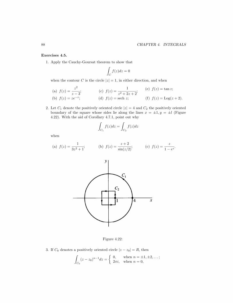
88 CHAPTER 4. INTEGRALS
Exercises 4.5.
1. Apply the Cauchy-Goursat theorem to show that∫C
f(z)dz = 0
when the contour C is the circle |z| = 1, in either direction, and when
(a) f(z) =z2
z − 3;
(b) f(z) = ze−z;
(c) f(z) =1
z2 + 2z + 2;
(d) f(z) = sech z;
(e) f(z) = tan z;
(f) f(z) = Log(z + 2).
2. Let C1 denote the positively oriented circle |z| = 4 and C2 the positively orientedboundary of the square whose sides lie along the lines x = ±1, y = ±l (Figure4.22). With the aid of Corollary 4.7.1, point out why∫
C1
f(z)dz =
∫C2
f(z)dz
when
(a) f(z) =1
3z2 + 1; (b) f(z) =
z + 2
sin(z/2); (c) f(z) =
z
1− ez.
Figure 4.22:
3. If C0 denotes a positively oriented circle |z − z0| = R, then∫C0
(z − z0)n−1dz =
{0, when n = ±1,±2, . . . ;2πi, when n = 0,

4.6. CAUCHY INTEGRAL FORMULA 89
according to Exercise 7. Use this result and Corollary 4.7.1 to show that if C isthe boundary of the rectangle 0 ≤ x ≤ 3, 0 ≤ y ≤ 2, described in the positivesense, then ∫
C
(z − 2− i)n−1dz =
{0, when n = ±1,±2, . . . ;2πi, when n = 0.
.
4.6 Cauchy Integral Formula
Theorem 4.8. (Cauchy Integral Formula) Let f be analytic everywhere inside andon a simple closed contour C and let z0 be an interior point of C. Then,
f(z0) =1
2πi
∫C
f(z)
z − z0dz.
Proof. Let Cρ denote a positively oriented circle |z − z0 = ρ|, where ρ is small enoughthat Cρ is interior to C (see Figure 4.23). Since the function f(z)/(z − z0) is analyticbetween and on the contours C and Cρ, it follows from the principle of deformation ofpaths (Corollary 4.7.1) that ∫
C
f(z)
z − z0dz =
∫Cρ
f(z)
z − z0dz
This enables us to write∫C
f(z)
z − z0dz − f(z0)
∫Cρ
dz
z − z0=
∫Cρ
f(z)− f(z0)
z − z0dz.
But from Exercise 7, ∫Cρ
dz
z − z0= 2πi;
and by substitution, we have∫C
f(z)
z − z0dz − 2πif(z0) =
∫Cρ
f(z)− f(z0)
z − z0dz.
Now the fact that f is analytic, and therefore continuous, at z0 ensures that, corre-sponding to each positive number ε, however small, there is a positive number δ suchthat
|f(z)− f(z0)| < ε whenever |z − z0| < δ.
Let the radius ρ of the circle C, be smaller than the number δ. Since |z − z0| = ρ whenz is onCρ, it follows that |f(z) − f(z0)| < ε holds when z is such a point; and fromTheorem 4.2 (5), we have∣∣∣∣∣
∫Cρ
f(z)− f(z0)
z − z0dz
∣∣∣∣∣ ≤ ε
ρ2πρ = 2πε.

90 CHAPTER 4. INTEGRALS
Hence, ∣∣∣∣∣∫C
f(z)
z − z0dz − 2πif(z0)
∣∣∣∣∣ < 2πε.
Since the left-hand side of this inequality is a nonnegative constant that is less than anarbitrarily small positive number, it must equal to zero. Hence the theorem is proved.
Figure 4.23:
The Cauchy Integral Formula tells us that if a function f is to be analytic withinand on a simple closed contour C, then the values of f interior to C are completelydetermined by the values of f on C.
When the Cauchy Integral Formula is written∫C
f(z)
z − z0dz = 2πif(z0) (4.9)
it can be used to evaluate certain integrals along simple closed contours.
Example 4.13. Find the value of the integral of f(z) around the circle |z| = 2 in the
positive sense when f(z) =z
9− z2.
Solution. Since f(z) is analytic within and on C and since the point z0 = −i is interiorto C, formula 4.9 tells us that∫
C
z
(9− z2)(z + i)dz =
∫C
z/9− z2
z − (−i))dz
= 2πi
(− i10
)
=π
5

4.7. DERIVATIVES OF ANALYTIC FUNCTIONS 91
4.7 Derivatives of Analytic Functions
It follows from the Cauchy Integral Formula that if a function is analytic at a point,then its derivatives of all orders exist at that point and are themselves analytic there.
Theorem 4.9. If a function is analytic at a point, then its derivatives of all orders existat that point. Those derivatives are, moreover, all analytic there.
We state the following theorem due to E. Morera (1856-1909). The proof here de-pends on the fact that the derivative of an analytic function is itself analytic, as statedin Theorem 4.9 .
Theorem 4.10. (Morera’s Theorem) Let f be continuous on a domain D. If∫C
f(z)dz = 0
for every closed contour C which lies in D, then f is analytic throughout D.
Proof. Suppose f be continuous on a domain D where
∫C
f(z)dz = 0 for every closed
contour C which lies in D. From Theorem 4.3, f has an antiderivative in D, that is,there exists an analytic function F such that F ′(z) = f(z) at each point in D. Since fis the derivative of F , it then follows from Theorem 4.9 that f is analytic in D.
Exercises 4.6.
1. Let C denote the positively oriented boundary of the square whose sides lie alongthe lines x = ±2 and y = ±2. Evaluate each of these integrals:
(a)
∫C
e−zdz
z − (πi/2);
(b)
∫C
cos z
z(z2 + 8)dz;
(c)
∫C
z
2z + 1dz;
(d)
∫C
cosh z
z4dz;
(e)
∫C
tan(z/2)
(z − x0)2dz,−2 <
x0 < 2.
2. Find the value of the integral of g(z) around the circle |z − i| = 2 in the positivesense when
(a) g(z) =1
z2 + 4; (b) g(z) =
1
(z2 + 4)2.
3. Let C be the circle |z| = 3, described in the positive sense. Show that if
g(w) =
∫C
2z2 − z − 2
z − wdz, |w| 6= 3,
then g(2) = 8πi. What is the value of g(w) when |w| > 3?

92 CHAPTER 4. INTEGRALS
4. Let C be any simple closed contour, described in the positive sense in the z plane,and write
g(w) =
∫C
z3 + 2z
(z − w)3dz.
Show that g(w) = 6πiw when w is inside C and that g(w) = 0 when w is outsideC.
5. Show that if f is analytic within and on a simple closed contour C and z0 is noton C, then ∫
C
f ′(z)
z − z0dz =
∫C
f(z)
(z − z0)2dz.
4.8 Liouville’s Theorem and the Fundamental Theo-rem of Algebra
This section is devoted to two important theorems that follow from the extension of theCauchy Integral formula.
Lemma 4.2. Suppose that a function f is analytic inside and on a positively orientedcircle CR, centered at z0 and with radius R (Fig. 67). If MR denotes the maximumvalue of |f(z)| on CR, then
|f (n)(z0)| ≤n!MR
Rn, n = 1, 2, . . . . (4.10)
Figure 4.24:
Inequality 4.10 is called Cauchy’s Inequality and is an immediate consequence of theexpression
f (n)(z0) =n!
2πi
∫CR
f(z)dz
(z − z0)n+1, n = 1, 2, . . . ,

4.8. LIOUVILLE’S THEOREMANDTHE FUNDAMENTAL THEOREMOF ALGEBRA93
From Theorem 4.2 (5), we have
|f (n)(z0)| ≤n!
2π·MR
Rn+12πR, n = 1, 2, . . . ,
where MR is as in the statement of the lemma.The lemma can be used to show that no entire function except a constant is bounded
in the complex plane. Our first theorem here, which is known as Liouville’s Theorem,states this result in a somewhat different way.
Theorem 4.11. (Liouville’s Theorem) If f is entire and bounded in the complexplane, then f(z) is constant throughout the plane.
Proof. We assume that f is entire and bounded in the complex plane. Since f is entire,Cauchy’s Inequality with n = 1 holds for any choices of z0 and R:
|f ′(z0)| ≤MR
R.
Moreover, since f is bounded, a nonnegative constant M exists such that |f(z)| < Mfor all z; and, because the constant MR is always less than or equal to M , it follows that
|f ′(z0)| ≤M
R.
where z0 is any fixed point in the plane and R is arbitrarily large. Now the number M is
independent of the value of R that is taken. Hence |f ′(z0)| ≤M
Rcan hold for arbitrarily
large values of R only if f ′(z0) = 0. Since the choice of z0 was arbitrary, this means thatf ′(z0) = 0 everywhere in the complex plane. Consequently, f is a constant function,according to Theorem 2.11.
The following theorem, known as the Fundamental Theorem of Algebra, follows read-ily from Liouville’s Theorem.
Theorem 4.12. (Fundamental Theorem of Algebra) Any polynomial
P (z) = a0 + a1z + a2z2 + . . .+ anz
n, an 6= 0
of degree n, n ≥ 1 has at least one zero. That is, there exists at least one point Z0 suchthat P (z0) = 0.
Proof. We prove by contradiction. Suppose that P (z) is not zero for any value of z.Then the reciprocal
f(z) =1
P (z)
is clearly entire, and it is also bounded in the complex plane.To show that it is bounded, we first write
w =a0
zn+
a1
zn−1+
a2
zn−2+ . . .+
an
z,

94 CHAPTER 4. INTEGRALS
so that P (z) = (an + w)zn. We then observe that a sufficiently large positive numberR can be found such that the modulus of each of the quotients is less than the number|an|/(2n) when |z| ≥ R. The generalized triangle inequality, applied to n complexnumbers, thus shows that |w| < |a|/2 for such values of z. Hence, when |z| > R,
|an + w| ≥ ||an| − |w|| >|an|
2;
and this enables us to write
|P (z)| = |an + w||zn| >|an|
2|zn| >
|an|2Rn whenever |z| ≥ R.
Therefore,
|f(z)| =1
|P (z)|<
2
|an|Rnwhenever |z| > R.
So f is bounded in the region exterior to the disk |z| ≤ R. But f is continuous in thatclosed disk, and this means that f is bounded there too. Hence f is bounded in theentire plane.
It now follows from Liouville’s Theorem that f(z), and consequently P (z) , is con-stant. ButP (z) is not constant, and we have reached a contradiction
Remark 4.2. The fundamental theorem tells us that any polynomial P (z) of degreen, n ≥ 1, can be expressed as a product of linear factors:
P (z) = c(z − z1)(z − z2) . . . (z − zn),
where c and zk, k = 1, 2, . . . , n, are complex constants. Some of the constants zk may,of course, appear more than once, and it is clear that P (z) can have no more than ndistinct zeros.

Chapter 5
SERIES
This chapter is devoted mainly to series representations of analytic functions. We presenttheorems that guarantee the existence of such representations, and we develop somefacility in manipulating series.
5.1 Convergence Of Sequences
Definition 5.1. A sequence of complex numbers
z1, z2, . . . , zn, . . .
, denoted by {zn} is a mapping from N to C, defined by
f : N → Cn → f(n) = zn.
Remark 5.1. In general,zn = xn + iyn,
where {xn} and {yn} are sequences of real numbers.
Definition 5.2. A infinite sequence of complex numbers {zn} is a has a limit z if, foreach positive number ε, there exists a positive integer N such that
|zn − z| < ε whenever n > N.
Geometrically, this means that, for sufficiently large values of n, the points z, lie inany given ε neighborhood of z (Fig. 71). Since we can choose ε as small as we please,it follows that the points zn become arbitrarily close to z as their subscripts increase.Note that the value of N that is needed will, in general, depend on the value of ε.
The sequence {zn} can have at most one limit. That is, a limit z is unique if it exists.When that limit exists, the sequence is said to converge to z; and we write
limn→∞
zn = z.
95

96 CHAPTER 5. SERIES
If the sequence has no limit, it diverges.
Figure 5.1:
Theorem 5.1. Suppose that zn = xn + iyn, (n = 1, 2, . . .) and z = x+ iy. Then
limn→∞
zn = z
if and only iflimn→∞
xn = x and limn→∞
yn = y.
Proof.(⇐) Suppose lim
n→∞xn = x and lim
n→∞yn = y. Hence, there exist positive integers N1 and
N2 such that
|xn − x| <ε
2whenever n > N1.
and
|yn − y| <ε
2whenever n > N2.
Hence, if N is the larger of the two integers N1 and N2,
|xn − x| <ε
2and |yn − y| <
ε
2whenever n > N.
Since
|(xn + iyn)− (x+ iy)| = |(xn − x) + i(yn − y)| ≤ |xn − x|+ |yn − y|,
then
|zn − z| <ε
2+ε
2whenever n > N.

5.1. CONVERGENCE OF SEQUENCES 97
Therefore,limn→∞
zn = z.
(⇒) Suppose limn→∞
zn = z. We know that, for each positive number ε, there exists a
positive integer N such that
|(xn + iyn)− (x+ iy)| < ε whenever n > N.
But|xn − x| ≤ |(xn − x) + i(yn − y)| = |(xn + iyn)− (x+ iy)|
and|yn − y| ≤ |(xn − x) + i(yn − y)| = |(xn + iyn)− (x+ iy)|;
which means that
|xn − x| < ε and |yn − y| < ε whenever n > N.
Thus,limn→∞
xn = x and limn→∞
yn = y.
Remark 5.2. The theorem enables us to write
limn→∞
(xn + iyn) = limn→∞
xn + i limn→∞
yn
whenever we know that both limits on the right exist or that the one on the left exists.
Example 5.1. Show that the sequence zn =1
n3+ i, (n = 1, 2, . . .) converges to i.
Solution.
limn→∞
zn = limn→∞
1
n3+ i
= limn→∞
1
n3+ i lim
n→∞1
= 0 + i · 1= i
Another way of showing this is to write
|zn − i| =1
n3,
and use the definition of limits to obtain the result. Hence, for each positive number ε,
|zn − i| < ε whenever n >13√ε.

98 CHAPTER 5. SERIES
Definition 5.3. A infinite series of complex numbers
∞∑n=1
zn = z1 + z2 + z3 + . . .+ zn + . . . ,
of complex numbers converges to the sum S if the sequence
SN =
N∑n=1
zn, N = 1, 2, . . .
of partial sums converges to S; we then write
∞∑n=1
zn = S
Note that, since a sequence can have at most one limit, a series can have at mostone sum. When a series does not converge, we say that it diverges.
Theorem 5.2. Suppose that zn = xn + iyn, (n = 1, 2, . . .) and S = X + iY . Then
∞∑n=1
zn = S
if and only if∞∑n=1
xn = X and
∞∑n=1
yn = Y.
Proof. we first write the partial sums as
SN = XN + iYN
where
XN =
N∑n=1
xn and YN =
N∑n=1
yn.
Now S =
∞∑n=1
zn if and only if
limN→∞
SN = S;
and this limit holds if and only if
limN→∞
XN = X and limN→∞YN = Y.
Therefore, limN→∞
SN = S, and conversely. Since XN and YN are the partial sums of the
series X and Y , respectively, the theorem here is proved.

5.1. CONVERGENCE OF SEQUENCES 99
Remark 5.3. This theorem tells us, of course, that one can write
∞∑n=1
(xn + iyn) =
∞∑n=1
xn + i
∞∑n=1
yn
whenever it is known that the two series on the right converge or that the one on the leftdoes.
By recalling from calculus that the nth term of a convergent series of real numbersapproaches zero as n tends to infinity, we can see immediately from the theorems dis-cussed that the same is true of a convergent series of complex numbers. That is, anecessary condition for the convergence of series is that
limn→∞
zn = 0.
The terms of a convergent series of complex numbers are, therefore, bounded. To bespecific, there exists a positive constant M such that |zn| ≤M for each positive integern.
Definition 5.4. A series
∞∑n=1
zn is absolutely convergent if the series
∞∑n=0
|zn| is con-
vergent.
Remark 5.4. Absolute convergence of a series of complex numbers implies convergenceof that series.
Exercises 5.1.
1. Show in two ways that the sequence
zn = −2 + i(−1)n
n2, n = 1, 2, . . .
converges to −2.
2. Show that
if limn→∞
zn = z, then limn→∞
|zn| = |z|.
3. Show that
if
∞∑n=1
zn = S, then
∞∑n=1
zn = S.
4. Let c denote any complex number and show that
if
∞∑n=1
zn = S, then
∞∑n=1
czn = cS.

100 CHAPTER 5. SERIES
5.2 Taylor Series
Theorem 5.3. (Taylor’s Series Formula) Suppose that a function f is analyticthroughout a disk |z − z0| < R0, centered at z0 and with radius R0. Then f(z) hasthe power series representation
f(z) =
∞∑n=0
an(z − z0)n, (|z − z0| < R0) (5.1)
where
an =f (n)(z0)
n!, n = 0, 1, 2, . . .
Figure 5.2:
Remark 5.5. If z0 = 0, then the Taylor series becomes
f(z) =
∞∑n=0
f (n)(0)
n!zn.
This is called the Maclaurin series.
Proof. We first prove the theorem when z0. Hence,
f(z) =
∞∑n=0
f (n)(0)
n!zn.
Let |z| = r and let C0 denote any positively oriented circle |z| = r0, where r < r0 < R0
(see Figure 5.3). Since f is analytic inside and on the circle C0 and since the point z isinterior to C0, the Cauchy integral formula applies:
f(z) =1
2πi
∫C0
f(s)ds
s− z.

5.2. TAYLOR SERIES 101
Now,
1
s− z=
1
s·
1
1− (z/s)
=1
s
[N−1∑n=0
(z
s
)n+
(z/s)N
1− (z/s)
]
=
N−1∑n=0
zn
sn+1+
zN
sN (s− z)
Multiplying each side by f(s) and then integrating each side with respect to s aroundC0, we have ∫
C0
f(s)ds
s− z=
N−1∑n=0
∫C0
f(s)ds
sn+1zn + zN
∫C0
f(s)ds
sN (s− z).
Multiplying both sides by 1/(2πi),
1
2πi
∫C0
f(s)ds
s− z=
N−1∑n=0
(1
2πi
∫C0
f(s)ds
sn+1
)zn +
zN
2πi
∫C0
f(s)ds
sN (s− z).
This gives us
f(z) =
N−1∑n=0
f (n)(0)
n!zn +
zN
2πi
∫C0
f(s)ds
sN (s− z).
We have to show that
limN→∞
(zN
2πi
∫C0
f(s)ds
sN (s− z)
)= 0.
Recall that |z| = r and that C0 has radius r0, where r0 > r. Then, if s is a point onC0, we can see that
|s− z| ≥ ||s| − |z|| = r0 − r.
Consequently, if M denotes the maximum value of |f(s)| on C0,∣∣∣∣∣ zN2πi
∫C0
f(s)ds
sN (s− z)
∣∣∣∣∣ ≤ rN
2π·
M
(r0 − r)rN02πr0 =
Mr0
r0 − r
(r
r0
)N.
Since (r/r0) < 1,then
limN→∞
(zN
2πi
∫C0
f(s)ds
sN (s− z)
)= 0
Now, when the disk of radius R0 is centered at an arbitrary point z0, we suppose thatf is analytic when |z− z0| < R0 and note that the composite function f(z+ z0) must beanalytic when |(z + z0)− z0| < R0, that is, |z| < R0. And if we write g(z) = f(z + z0),

102 CHAPTER 5. SERIES
the analyticity of g in the disk |z| < R0 ensures the existence of a Maclaurin seriesrepresentation:
g(z) =
∞∑n=0
g(n)(0)
n!zn, (|z| < R0).
That is,
f(z + z0) =
∞∑n=0
f (n)(z0)
n!zn, (|z| < R0).
This gives us the desired Taylor series expansion 5.1.
Figure 5.3:
Example 5.2. Obtain the Maclaurin series representation
1. ez =
∞∑n=0
zn
n!, (|z| <∞);
2. z2e3z =
∞∑n=2
3n−2
(n− 2)!zn, (|z| <∞).
Solution.
1. Since f (n)(z) = ez, we have f (n)(0) = 1. Hence,
ez =
∞∑n=0
f (n)(0)
n!zn =
∞∑n=0
zn
n!.

5.2. TAYLOR SERIES 103
2. We have
ez =
∞∑n=0
zn
n!
e3z =
∞∑n=0
(3z)n
n!
z2e3z =
∞∑n=0
3n
n!zn+2
z2e3z =
∞∑n=2
3n−2
(n− 2)!zn
Example 5.3. Obtain the Maclaurin series representation for f(z) = sin z.Solution. Recall that
sin z =eiz − e−iz
2i.
Hence,
sin z =1
2i
[ ∞∑n=0
(iz)n
n!−∞∑n=0
(−iz)n
n!
]
=1
2i
∞∑n=0
[1− (−1)n]inzn
n!
=1
2i
∞∑n=0
[1− (−1)2n+1]i2n+1z2n+1
(2n+ 1)!since 1− (−1)n = 0 when n is even
=1
2i
∞∑n=0
2(−1)niz2n+1
(2n+ 1)!
=∞∑n=0
(−1)nz2n+1
(2n+ 1)!
Example 5.4. Obtain the Maclaurin series representation for f(z) = cos z.Solution. Since
sin z =
∞∑n=0
(−1)nz2n+1
(2n+ 1)!
, we obtain the Maclaurin series expansion for cos z by differentiating each side of thisequation. Hence,
cos z =
∞∑n=0
(−1)n2n+ 1
(2n+ 1)!z2n =
∞∑n=0
(−1)nz2n
(2n)!.
Example 5.5. Obtain the Maclaurin series representation for f(z) = sinh z.

104 CHAPTER 5. SERIES
Solution. Sincesinh z = −i sin(iz)
and
sin z =
∞∑n=0
(−1)nz2n+1
(2n+ 1)!,
we obtain the Maclaurin series expansion for sinh z by first replacing z by iz on eachside of this equation.
sin(iz) =
∞∑n=0
(−1)n(iz)2n+1
(2n+ 1)!
−i sin(iz) =
∞∑n=0
(−1)n − i(iz)2n+1
(2n+ 1)!
sinh z =
∞∑n=0
(−1)n(z)2n+1
(2n+ 1)!
Example 5.6. Obtain the Maclaurin series representation
1.1
1− z=
∞∑n=0
zn, (|z| < 1);
2.1
1 + z=
∞∑n=0
(−1)nzn, (|z| < 1).
Solution.
1. Let f(z) =1
1− z= (1− z)−1.
f ′(z) = (1− z)−2
f ′′(z) = 2(1− z)−3
f ′′′(z) = 6(1− z)−4
... =...
f (n)(z) = n!(1− z)−(n+1)
Since f (n)(0) = n!, then
1
1− z=
∞∑n=0
f (n)(0)
n!zn =
∞∑n=0
n!
n!zn =
∞∑n=0
zn.
2. Given1
1− z=
∞∑n=0
zn, we substitute −z to z.
1
1 + z=
∞∑n=0
(−z)n, (|z| < 1) =
∞∑n=0
(−1)nzn, (|z| < 1).

5.2. TAYLOR SERIES 105
Remark 5.6. If we replace z by (1 − z) in1
1− z=
∞∑n=0
zn, we have the Taylor series
representation
1
z=
∞∑n=0
(−1)n(z − 1)n, (|z − 1| < 1).
Example 5.7. Expand the function
f(z) =1 + 2z2
z3 + z5
into a series involving powers of z.Solution. We note that f(z) is not analytic at z = 0.
f(z) =1 + 2z2
z3 + z5
=1 + 2z2
z3(1 + z2)
=2 + 2z2 − 1
z3(1 + z2)
=2(1 + z2)− 1
z3(1 + z2)
=2(1 + z2)
z3(1 + z2)−
1
z3(1 + z2)
=2
z3−
1
z3(1 + z2)
=2
z3−
1
z3·
1
1 + z2
=2
z3−
1
z3
∞∑n=0
(−z2)n, |z| < 1
=2
z3−
1
z3
∞∑n=0
(−1)nz2n
=2
z3−∞∑n=0
(−1)nz2n−3
Exercises 5.2.
1. Obtain the Maclaurin series representation
z cosh(z2) =
∞∑n=0
z4n+1
(2n)!, (|z| <∞)

106 CHAPTER 5. SERIES
2. Obtain the Taylor series
ez = e
∞∑n=0
(z − 1)n
n!, (|z − 1| <∞)
for the function f(z) = ez by
(a) using f (n)(1), (n = 0, 1, 2, . . .); (b) writing ez = ez−1e.
3. Find the Maclaurin series expansion of the function
f(z) =z
z4 + 9=z
9·
1
1 + (z4/9)
4. Show that if f(z) = sin z, then
f (2n)(0) = 0 and f (2n+1)(0) = (−1)n, n = 0, 1, 2, . . . .
and give an alternative derivation of the Maclaurin series for sin z.
5. Derive the Maclaurin series for the function f(z) = cos z by
(a) using the definition
cos z =eiz + e−iz
2;
(b) showing that
f (2n)(0) = (−1)n and f (2n+1)(0) = 0, n = 0, 1, 2, . . . .
6. Write the Maclaurin series representation of the function f(z) = sin(z2), and pointout how it follows that
f (4n)(0) = 0 and f (2n+1)(0) = 0, n = 0, 1, 2, . . . .
7. Derive the Taylor series representation
1
1− z=
∞∑n=0
(z − i)n
(1− i)n+1, (|z − i| <
√2).
Suggestion: Start by writing
1
1− z=
1
(1− i)− (z − i)=
1
1− i·
1
1− (z − i)/(1− i).

5.3. LAURENT SERIES 107
5.3 Laurent Series
If a function f fails to be analytic at a point z0, we cannot apply Taylor’s theoremat that point. It is often possible, however, to find a series representation for f(z)involving both positive and negative powers of z − z0. We now present the theory ofsuch representations, and we begin with Laurent’s theorem.
Theorem 5.4. (Laurent’s Theorem) Suppose that a function f is analytic throughoutan annular domain R1 < |z − z0| < R2, centered at z0, and let C denote any positivelyoriented simple closed contour around z0 and lying in that domain (Figure 5.4). Then,at each point in the domain, f(z) has the series representation
f(z) =
∞∑n=0
an(z − z0)n +
∞∑n=1
bn
(z − z0)n, (R1 < |z − z0| < R2), (5.2)
where
an =1
2πi
∫C
f(z)dz
(z − z0)n+1and bn =
1
2πi
∫C
f(z)dz
(z − z0)−n+1, n = 0, 1, 2, . . . .
The series in Equation 5.2 is called the Laurent series of f about z0 and the series∞∑n=1
bn
(z − z0)nis called the principal part of f .
Figure 5.4:

108 CHAPTER 5. SERIES
Remark 5.7. The Laurent series can also be written as
f(z) =
∞∑n=−∞
cn(z − z0)n, (R1 < |z − z0| < R2),
where
cn =1
2πi
∫C
f(z)dz
(z − z0)n+1, n = 0,±1,±2, . . . .
Proof. We start the proof by forming a closed annular region r1 ≤ |z| ≤ r2 that iscontained in the domain R1 < |z| < R2 and whose interior contains both the pointz and the contour C (Figure 5.5). We let C1 and C2 denote the circles |z| = r1 and|z| = r2, respectively, and we assign those two circles a positive orientation. Observethat f is analytic on C1 and C2, as well as in the annular domain between them.
Next, we construct a positively oriented circle γ with center at z and small enoughto be completely contained in the interior of the annular region r1 ≤ |z| ≤ r2, as shownin Figure 5.5. It then follows from the extension of the Cauchy-Goursat Theorem (The-orem 4.6 to integrals of analytic functions around the oriented boundaries of multiplyconnected domains that∫
C2
f(s)ds
s− z−∫C1
f(s)ds
s− z−∫γ
f(s)ds
s− z= 0
But, according to the Cauchy Integral Formula,
∫γ
f(s)ds
s− z= 2πif(z) . Hence
f(z) =1
2πi
∫C2
f(s)ds
s− z+
1
2πi
∫C1
f(s)ds
z − s
From the proof of Taylor’s Series Formula,
1
s− z=
N−1∑n=0
zn
sn+1+
zN
sN (s− z).
This gives us
1
z − s=
N−1∑n=0
sn
zn+1+
sN
zN (z − s)
=
N−1∑n=0
1
s−n·
1
zn+1+
1
zN·sN
z − s
=
N∑n=1
1
s−n+1·
1
zn+
1
zN·sN
z − s

5.3. LAURENT SERIES 109
Now,
f(s)
2πi·
1
s− z=
f(s)
2πi
N−1∑n=0
zn
sn+1+
zN
sN (s− z)
1
2πi
∫C2
f(s)ds
s− z=
1
2πi
∫C2
[N−1∑n=0
f(s)zn
sn+1+
f(s)zN
sN (s− z)
]ds
and
f(s)
2πi·
1
z − s=
f(s)
2πi·N∑n=1
1
s−n+1·
1
zn+
1
zN·sN
z − s
1
2πi
∫C1
f(s)ds
z − s=
1
2πi
∫C1
[N∑n=1
f(s)
s−n+1·
1
zn+
1
zN·f(s)sN
z − s
]ds
Hence,
f(z) =1
2πi
∫C2
f(s)ds
s− z+
1
2πi
∫C1
f(s)ds
z − s
=1
2πi
∫C2
[N−1∑n=0
f(s)zn
sn+1+
f(s)zN
sN (s− z)
]ds+
1
2πi
∫C1
[N−1∑n=1
f(s)
s−n+1·
1
zn+
1
zN·f(s)sN
z − s
]ds
=
N−1∑n=0
anzn +
zN
2πi
∫C2
f(s)ds
sN (s− z)+
N∑n=1
bn
zn+
1
2πizN
∫C1
f(s)sNds
z − s
where
an =1
2πi
∫C2
f(s)ds
sn+1, n = 0, 1, . . . , N − 1 and bn =
1
2πi
∫C1
f(s)ds
s−n+1, n = 1, 2, . . . , N.
Now, we let
ρn(z) =zN
2πi
∫C2
f(s)ds
sN (s− z)and σn(z) =
1
2πizN
∫C1
f(s)sNds
z − s.
We have to show that
limn→∞
ρn(z) = 0and and limn→∞
σn(z) = 0
We write |z| = r, so that r1 < r < r2, and letM denote the maximum value of |f(s)| onC1 and C2. We also note that if s is a point on C2, then |s− z| ≥ r2 − r; and if s is onC1, |s− z| ≥ r − r1. This enables us to write
|ρn(z)| ≤Mr2
r2 − r
(r
r2
)Nand |σn(z)| ≤
Mr1
r − r1
(r1
r
)N.

110 CHAPTER 5. SERIES
Since (r/r2) < 1 and (r1/r) < 1, it follows that
limn→∞
ρn(z) = 0 and limn→∞
σn(z) = 0
Therefore,
f(z) =
N−1∑n=0
anzn +
N∑n=1
bn
zn
Now, from Corollary 4.7.1, we can replace the contours C1 and C2 by C and when z0 = 0we have
f(z) =
∞∑n=0
anzn +
∞∑n=1
bn
zn,
where z is used instead of s as the variable of integration.To extend the proof to the general case in which z0 is an arbitrary point in the finite
plane, we let f be a function satisfying the conditions in the theorem; and, just as wedid in the proof of Taylor’s Series Formula, we write g(z) = f(z + z0). Since f(z) isanalytic in the annulus R1 < |z − z0| < R2, the function f(z + z0) is analytic whenR1 < |(z + z0)− z0| < R2. That is, g is analytic in the annulus R1 < |z| < R2, which iscentered at the origin. Now the simple closed contour C in the statement of the theoremhas some parametric representation z = z(t), (a ≤ t ≤ b), where
R1 < |z(t)− z0| < R2
for all t in the interval a ≤ t ≤ b. Hence if Γ denotes the path
z = z(t)− z0, a ≤ t ≤ b
Γ is not only a simple closed contour but, it lies in the domain R1 < |z| < R2 sinceR1 < |z(t)− z0| < R2. Consequently, g(z) has a Laurent series representation
g(z) =
∞∑n=0
anzn +
∞∑n=1
bn
zn, R1 < |z| < R2,
where
an =1
2πi
∫Γ
g(z)dz
zn+1, n = 0, 1, 2, . . . and bn =
1
2πi
∫Γ
g(z)dz
z−n+1, n = 1, 2, . . . .
If we write f(z + z0) instead of g(z and then replace z by z − z0 in the resultingequation, as well as in the condition of validity R1 < |z| < R2 we obtain
f(z) =
∞∑n=0
an(z − z0)n +
∞∑n=1
bn
(z − z0)n, (R1 < |z − z0| < R2),
where
an =1
2πi
∫C
f(z)dz
(z − z0)n+1and bn =
1
2πi
∫C
f(z)dz
(z − z0)−n+1, n = 0, 1, 2, . . . .

5.3. LAURENT SERIES 111
This is because
an =1
2πi
∫Γ
g(z)dz
zn+1=
1
2πi
∫ b
a
f [(z(t)]z′(t)
[z(t)− z0]n+1dt =
∫C
f(z)dz
(z − z0)n+1
and
bn =1
2πi
∫Γ
g(z)dz
z−n+1=
1
2πi
∫ b
a
f [(z(t)]z′(t)
[z(t)− z0]−n+1dt =
1
2πi
∫C
f(z)dz
(z − z0)−n+1.
Figure 5.5:
Example 5.8. Find the Laurent series that represents the function
f(z) = e1/z
in the domain 0 < |z| <∞.Solution. We know that
ez =
∞∑n=0
zn
n!, |z| <∞.
We replace z by 1/z.
e1/z =
∞∑n=0
(1/z)n
n!
=
∞∑n=0
1
n!zn, 0 < |z| <∞

112 CHAPTER 5. SERIES
Note that no positive powers of z appear here, the coefficients of the positive powersbeing zero. Note, too, that the coefficient of l/z is unity; and, according to Laurent’sTheorem, that coefficient is the number
b1 =1
2πi
∫C
e1/zdz,
where C is any positively oriented simple closed contour around the origin. Since b1 = 1,then, ∫
C
e1/zdz = 2πi.
Example 5.9. Write the two Laurent series in powers of z that represent the function
f(z) =− 1
(z − 1)(z − 2)
in certain domains, and specify those domains.
Solution. The function f(z) has the two singular points z = 1 and z = 2, is analyticin the domains
|z| < 1, 1 < |z| < 2, and 2 < |z| <∞.
In each of those domains, denoted by D1, D2, and D3, respectively, in Figure5.6, f(z)has series representations in powers of z.
Figure 5.6:

5.3. LAURENT SERIES 113
Case 1. D1 : |z| < 1
f(z) =− 1
(z − 1)(z − 2)
=1
z − 1−
1
z − 2
= −1
1− z+
1
2(1− (z/2), |z| < 1, |z/2| < 1
= −∞∑n=0
zn +
∞∑n=0
zn
2n+1
=
∞∑n=0
1− 2n+1
2n+1zn
Case 2. D2 : 1 < |z| < 2
f(z) =− 1
(z − 1)(z − 2)
=1
z(1− (1/z)+
1
2(1− (z/2), |1/z| < 1, |z/2| < 1
=1
z
∞∑n=0
(1
z
)n+
1
2
∞∑n=0
(z
2
)nCase 3. D3 : |z| > 2
f(z) =− 1
(z − 1)(z − 2)
=1
z(1− (1/z)−
1
z(1− (2/z), |1/z| < 1, |2/z| < 1
=1
z
∞∑n=0
(1
z
)n−
1
z
∞∑n=0
(2
z
)n
=
∞∑n=0
1
zn+1−∞∑n=0
2n
zn+1
Exercises 5.3.
1. Find the Laurent series that represents the function
f(z) = z2 sin
(1
z2
)
in the domain 0 < |z| <∞.

114 CHAPTER 5. SERIES
2. Derive the Laurent series representation
ez
(z = 1)2=
1
e
[ ∞∑n=0
(z + 1)n
(n+ 2)!+
1
z + 1+
1
(z + 1)2
], (0 < |z| <∞)
3. Find a representation for the function
f(z) =1
1 + z=
1
z·
1
1 + (1/z)
in negative powers of z that is valid when 1 < |z| <∞.
4. Give two Laurent series expansions in powers of z for the function
f(z) =1
z2(1− z),
and specify the regions in which those expansions are valid.
5. Represent the function
f(z) =z + 1
z − 1
(a) by its Maclaurin series, and state where the representation is valid;
(b) by its Laurent series in the domain 1 < |z| <∞.
6. Show that when 0 < |z − 1| < 2,
z
(z − 1)(z − 3)= −3
∞∑n=0
(z − 1)n
2n+2−
1
2(z − 1).
7. Write the two Laurent series in powers of z that represent the function
f(z) =1
z(1 + z2)
in certain domains, and specify those domains.
Chapter 6
RESIDUES AND POLES
The Cauchy-Goursat Theorem states that if a function is analytic at all points interiorto and on a simple closed contour C, then the value of the integral of the function aroundthat contour is zero. If, however, the function fails to be analytic at a finite number ofpoints interior to C, there is, as we shall see in this chapter, a specific number, called aresidue, which each of those points contributes to the value of the integral. We develophere the theory of residues.
6.1 Residues
Recall that a point z0 is called a singular point of a function f if f fails to be analyticat z0 but is analytic at some point in every neighborhood of z0. A singular point z0 issaid to be isolated if, in addition, there is a deleted neighborhood 0 < |z − z0| < ε of z0
throughout which f is analytic.
Example 6.1. Find the singular points of the function
z + 1
z3(z2 + 1).
Solution. The three isolated singular points are z = 0 and z = ±i.
Example 6.2. Find the singular point of the logarithmic function
Log z.
Solution. The origin is a singular point of the principal branch
Log z = ln r + iΘ, (r > 0,−π < Θ < π).
It is not, however, an isolated singular point since every deleted ε neighborhood of itcontains points on the negative real axis (see Figure 6.1) and the branch is not evendefined there.
115

116 CHAPTER 6. RESIDUES AND POLES
Figure 6.1:
Example 6.3. Find the singular point of the function
1
sin(π/z).
Solution. The function1
sin(π/z)
has the singular points z = 0 and z =1
n(n = ±1,±2, . . .), all lying on the segment of
the real axis from z = −1 to z = 1. Each singular point except z = 0 is isolated. Thesingular point z = 0 is not isolated because every deleted ε neighborhood of the origincontains other singular points of the function. More precisely, when a positive number εis specified and m is any positive integer such that m > 1/ε, the fact that 0 < 1/m < εmeans that the point z = 1/m lies in the deleted ε neighborhood 0 < |z| < ε (Figure 6.2).
Figure 6.2:

6.1. RESIDUES 117
Suppose z0 is an isolated singular point of a function f . There exists a positivenumber number R > 0, such that the Laurent series of f at z0 is given by Equation 5.2.Consider the principal part of this series, that is, the expression
∞∑n=1
bn
(z − z0)n=
b1
z − z0+
b2
(z − z0)2+ . . .+
bn
(z − z0)n+ . . . . (6.1)
The coefficients bn is given by
bn =1
2πi
∫C
f(z)dz
(z − z0)−n+1, n = 1, 2, . . . ,
where C is any positively oriented simple closed contour around z0 and lying in thepunctured disk 0 < |z − z0| < R (Figure 6.3). When n = 1, this expression for bn, canbe written ∫
C
f(z)dz = 2πib1. (6.2)
Figure 6.3:
Definition 6.1. The coefficient b1 given in Equation 6.1, that is the coefficient of1
z − z0in Equation 6.1 is called the residue of f at the isolated singular point z0. We will denoteby
Bk = Resz=zkf(z),
the residue of f at the isolated singular point zk of f .
Remark 6.1. Equation 6.2 can be used to evaluate certain integrals around simple closedcontours.
Example 6.4. Evaluate ∫C
dz
z(z − 2)4

118 CHAPTER 6. RESIDUES AND POLES
where C is the positively oriented circle |z − 2| = 1 (Figure 6.4).
Figure 6.4:
Solution.
f(z) =1
z(z − 2)4
=1
(z − 2)4·
1
z
=1
(z − 2)4·
1
(z − 2) + 2
=1
(z − 2)4·
1
2(1 + (z − 2)/2)
=1
(z − 2)4·∞∑n=0
(−1)n
(z − 2
2
)n
=
∞∑n=0
(−1)n(z − 2)n−4
2n+1
In this Laurent series, the coefficient of 1/(z−2) is the desired residue where n−4 = −1.This gives us n = 3 and we have
Resz=2f(z) =(−1)n
2n+1=
(−1)3
24= −
1
16
Consequently, ∫C
dz
z(z − 2)4= 2πi
(−
1
16
)= −
πi
8
Example 6.5. Evaluate ∫C
exp
(1
z2
)dz
where C is the unit circle |z| = 1 .

6.2. CAUCHY’S RESIDUE THEOREM 119
Solution. The function f(z) = e1/z2 has an isolated singularity at z = 0.
exp
(1
z2
)=
∞∑n=0
(1/z2)n
n!
=
∞∑n=0
1
z2nn!
= 1 +1
z2+
1
2z4+
1
6z6+ . . .
The desired residue is Resz=0f(z) = 0. Therefore,∫C
exp
(1
z2
)dz = 0
6.2 Cauchy’s Residue Theorem
If, except for a finite number of singular points, a function f is analytic inside a simpleclosed contour C, those singular points must be isolated. The following theorem, whichis known as Cauchy’s Residue Theorem, is a precise statement of the fact that if f isalso analytic on C and if C is positively oriented, then the value of the integral of faround C is 2πi times the sum of the residues of f at the singular points inside C.
Theorem 6.1. (Cauchy’s Residue Theorem) Let C be a positively oriented simpleclosed contour. If the function f is analytic inside and on C except for a finite numberof singular points zk, k = 1, 2, . . . n inside C, then
∫C
f(z)dz = 2πi
n∑k=1
Resz=zkf(z). (6.3)
Proof. let the points zk, k = 1, 2, . . . n, be centers of positively oriented circles Ck whichare interior to C and are so small that no two of them have points in common (Figure6.5). The circles Ck, together with the simple closed contour C, form the boundary of aclosed region throughout which f is analytic and whose interior is a multiply connecteddomain. Hence, according to Theorem 4.6∫
C
f(z)dz −n∑k=1
∫Ck
f(z)dz = 0.
Since ∫Ck
f(z)dz = 2πiResz=zkf(z), k = 1, 2, . . . , n
we have ∫C
f(z)dz = 2πi
n∑k=1
Resz=zkf(z).

120 CHAPTER 6. RESIDUES AND POLES
Figure 6.5:
Example 6.6. Use Theorem 6.3 to evaluate the integral
∫C
5z − 2
z(z − 1)dz,
when C is the circle |z| = 2 oriented in a counterclockwise manner.
Solution. The function f(z) =5z − 2
z(z − 1)has isolated singularities at z = 0 and z = 1
which are both inside C. By Theorem 6.3
∫C
5z − 2
z(z − 1)dz = 2πi [Resz=0f(z) +Resz=1f(z)]
First we find Resz=0f(z).
5z − 2
z(z − 1)=
5z − 2
z·
1
z − 1
=
(5−
2
z
)(−1) ·
1
1− z
=
(−5 +
2
z
) ∞∑n=0
zn
=
(−5 +
2
z
)(1 + z + z2 + . . .)
Hence, Resz=0f(z) = 2

6.2. CAUCHY’S RESIDUE THEOREM 121
Figure 6.6:
Next we find Resz=1f(z).
5z − 2
z(z − 1)=
1
z − 1·
5z − 2
z
=1
z − 1·
(5−
2
z
)
=1
z − 1·
(5−
2
z − 1 + 1
)
=1
z − 1·
(5−
2
1 + (z − 1)
)
=1
z − 1·
(5− 2
∞∑n=0
(−1)n(z − 1)n
)
=5
z − 1− 2
∞∑n=0
(−1)n(z − 1)n−1
=5
z − 1− 2
[1
z − 1− 1 + (z − 1)− (z − 1)2 + . . .
]
=3
z − 1+ 2− 2(z − 1) + 2(z − 1)2 − . . .
Hence, Resz=1f(z) = 3. Therefore,∫C
5z − 2
z(z − 1)dz = 2πi [Resz=0f(z) +Resz=1f(z)] = 2πi(2 + 3) = 10πi

122 CHAPTER 6. RESIDUES AND POLES
Exercises 6.1.
1. Find the residue at z = 0 of the function
(a)1
z + z2; (b) 2 cos
(1
z
); (c)
z − sin z
z; (d)
cot z
z4; (e)
sinh z
z4(1− z2).
2. Use Cauchy’s Residue Theorem to evaluate the integral of each of these functionsaround the circle |z| = 3 in the positive sense:
(a)exp(−z)z2
; (b)exp(−z)(z − 1)2
; (c) z2 exp
(1
z
); (d)
z + 1
z2 − 2z.
6.3 Three Types of Isolated Singular Points
Consider the principal part of the Laurent series expansion of f(z) about the the isolatedsingular point z0 of f given in Equation 6.1. Suppose, this expansion is finite, that isthere is an integer m such that bm 6= 0 and bm+1 = bm+2 = · · · = 0 and Equation 6.1takes the form
∞∑n=1
bn
(z − z0)n=
b1
z − z0+
b2
(z − z0)2+ . . .+
bm
(z − z0)m,
where bm 6= 0. Then, we say that the isolated singular point z0 is a pole of order m. Ifm = 1, then z0 is called a simple pole.
Example 6.7. Let
f(z) =z2 − 2z + 3
z − 2, 0 < |z − 2| <∞.
Show that f(z) has a simple pole at z0 = 2 with residue b1 = 3.Solution.
z2 − 2z + 3
z − 2=
z(z − 2) + 3
z − 2
= z +3
z − 2
= 2 + (z − 2) +3
z − 2, 0 < |z − 2| <∞
Hence, f(z) has a simple pole at z0 = 2 with residue b1 = 3.
Example 6.8. Let
f(z) =sinh z
z4, 0 < |z| <∞.
Show that f(z) has a pole z0 = 0 of order 3 with residue b1 =1
6.

6.3. THREE TYPES OF ISOLATED SINGULAR POINTS 123
Solution.
sinh z
z4=
1
z4
∞∑n=0
(−1)n(z)2n+1
(2n+ 1)!
=1
z4
(z +
z3
3!+z5
5!+z7
7!+ . . .
)
=1
z3+
1
3!z+z
5!+z3
7!+ . . . , 0 < |z| <∞
Hence, f(z) has a pole z0 = 0 of order 3 with residue b1 =1
6.
If in the Laurent series expansion of f , the principal part vanishes, that is b1 = b2 =. . . = 0, then we say that the isolated singular point z0 of f is a removable singularpoint. The residue at a removable singular point is always zero. If we redefine f at z0,say f(z0) = a0, then the singularity of f at z0 is removed.
Example 6.9. Let
f(z) =1− cos z
z2, 0 < |z| <∞.
Show that f has a removable singular point at z0 = 0.Solution.
1− cos z
z2=
1
z2(1− cos z)
=1
z2
[1−
∞∑n=0
(−1)nz2n
(2n)!
]
=1
z2
[1−
(1−
z2
2!+z4
4!−z6
6!+ . . .
)]
=1
2!− cfracz24! +
z4
6!− . . . , 0 < |z| <∞.
When the value f(0) = 1/2 is assigned, f becomes entire.
If in the Laurent series expansion of f , the principal part is infinite, that is, aninfinite number of coefficients bn is infinite, then the isolated singular point z0 is said tobe an essential singular point of f .
An important result concerning the behavior of a function near an essential singularpoint is due to Picard.
Theorem 6.2. (Picard’s Theorem) In each neighborhood of an essential singularpoint, a function assumes every finite value, with one possible exception, an infinitenumber of times.

124 CHAPTER 6. RESIDUES AND POLES
Example 6.10. Let
f(z) = exp
(1
z
), 0 < |z| <∞.
Show that f has an essential singular point at z0 = 0, where the residue b1 is unity.Solution. For an illustration of Picard’s Theorem, let us show that exp(1/z) assumesthe value −1 an infinite number of times in each neighborhood of the origin. Recall thatexp z = −1 when z = (2n + 1)πi, (n = 0,±1,±2, . . .). This means that exp(l/z) = −1when
z =1
(2n+ 1)πi·i
i
= −1
(2n+ 1)π
and an infinite number of these points clearly lie in any given neighborhood of the origin.Since exp(1/z) 6= 0 for any value of z, zero is the exceptional value in Picard’s Theorem.
Exercises 6.2.
1. In each case, write the principal part of the function at its isolated singular pointand determine whether that point is a pole, a removable singular point, or anessential singular point:
(a) z exp
(1
z
); (b)
z2
1 + z; (c)
sin z
z; (d)
cos z
z; (e)
1
(2− z)3.
2. Show that the singular point of each of the following functions is a pole. Determinethe order m of that pole and the corresponding residue b1.
(a)1− cosh z
z3; (b)
1− exp(2z)
z4; (c)
exp(2z)
(z − 1)2.
3. Suppose that a function f is analytic at z0, and write g(z) = f(z)/(z − z0) Showthat
(a) if f(z0) 6= 0, then z0 is a simple pole of g, with residue f(z0);
(b) if f(z0) = 0, then z0 is a removable singular point of g.
Suggestion: Recall that there is a Taylor series for f(z) about z0 since f is analyticthere. Start each part of this exercise by writing out a few terms of that series.
6.4 Residues at Poles
When a function f has an isolated singularity at a point z0, the basic method for identi-fying z0 as a pole and finding the residue there is to write the appropriate Laurent seriesand to note the coefficient of 1/(z − z0). The following theorem provides an alternativecharacterization of poles and another way of finding the corresponding residues.

6.4. RESIDUES AT POLES 125
Theorem 6.3. An isolated singular point z0 of a function f is a pole of order m if andonly if f(z) can be written in the form
f(z) =φ(z)
(z − z0)m,
where φ(z) is analytic and φ(z0) 6= 0. Moreover,
Resz=z0f(z) =φ(m−1)(z0)
(m− 1)!,m ≥ 1. (6.4)
Proof.
(⇐) Suppose f(z) =φ(z)
(z − z0)m, where φ(z) is analytic and φ(z0) 6= 0. Recall that since
φ(z) is analytic at z0, it has a Taylor series representation
φ(z) = φ(z0)+φ′(z0)
1!(z−z0)+
φ′′(z0)
2!(z−z0)2+. . .+
φ(m−1)(z0)
(m− 1)!(z−z0)m−1+
∞∑n=m
φ(n)(z0)
n!(z−z0)n
in some neighborhood |z − z0| < ε of z0; and it follows that
f(z) =φ(z0)
(z − z0)m+
φ′(z0)/1!
(z − z0)m−1+
φ′′(z0)/2!
(z − z0)m−2+. . .+
φ(m−1)(z0)/(m− 1)!
z − z0+
∞∑n=m
φ(n)(z0)
n!(z−z0)n−m
when |z − z0| < ε. This Laurent series representation, together with the fact thatφ(z0) 6= 0, reveals that z0 is, indeed, a pole of order m of f(z). The coefficient of1/(z − z0) tells us that the residue of f(z) at zo is
Resz=z0f(z) =φ(m−1)(z0)
(m− 1)!,m ≥ 1.
(⇒) Suppose that we know only that z0 is a pole of order m of f , or that f(z) has aLaurent series representation
f(z) =
∞∑n=0
an(z − z0)n +b1
z − z0+
b2
(z − z0)2+ . . .+
bm−1
(z − z0)m−1+
bm
(z − z0)m, bm 6= 0
which is valid in a punctured disk 0 < |z− z0| < R. The function φ(z) defined by meansof the equations
φ(z) =
{(z − z0)mf(z), when z 6= z0,bm, when z = z0
has the power series representation
φ(z) = bm + bm−1(z − z0) + . . .+ b2(z − z0)m−2 + b1(z − z0)m−1 +
∞∑n=0
an(z − z0)m+n
126 CHAPTER 6. RESIDUES AND POLES
throughout the entire disk |z − z0| < R . Hence, φ(z) is analytic in that disk and, inparticular, at z0. Since φ(z0) = bm 6= 0 we have
f(z) =φ(z)
(z − z0)m.
Example 6.11. Find the poles and the corresponding residues of the following functions.
1. f(z) =z + 1
z2 + 9; 2. f(z) =
z3 + 2z
(z − i)3.
Solution.
1. The function f(z) =z + 1
z2 + 9has an isolated singular point at z = 3i and can be
written as
f(z) =φ(z)
z − 3iwhere φ(z) =
z + 1
z + 3i.
Since φ(z) is analytic at z = 3i and φ(3i) = (3 − i)/6 6= 0, that point is a simplepole of the function f ; and the residue there is B1 = (3− i)/6. The point z = −3iis also a simple pole of f , with residue B2 = (3 + i)/6.
2. If f(z) =z3 + 2z
(z − i)3, then
f(z) =φ(z)
(z − i)3where φ(z) = z3 + 2z.
The function φ(z) is entire, and φ(i) = i 6= 0. Hence f has a pole of order 3 at
z = i. The residue there isφ′′(i)
2!= 3i.
Before we end this section we cite this theorem which will be used in the next section.
Theorem 6.4. Let two functions p and q be analytic at a point z0. If
p(z0) 6= 0, q(z0) = 0, and q′(z0) 6= 0
then
Resz=z0p(z)
q(z)=
p(z0)
q′(z0).

6.4. RESIDUES AT POLES 127
Exercises 6.3.
1. In each case, show that any singular point of the function is a pole. Determine theorder m of each pole, and find their corresponding residues.
(a)z2 + 2
z − 1; (b)
(z
2z + 1
)3
; (c)exp z
z2 + π2.
2. Show that
(a) Resz=−1
z1/4
z + 1=
1 + i√
2, (|z| > 0, 0 < arg z < 2π);
(b) Resz=iLog z
(z2 + 1)2=π + 2i
8;
(c) Resz=iz1/2
(z2 + 1)2=
1− i8√
2, (|z| > 0, 0 < arg z < 2π).
3. Find the value of the integral∫C
3z3 + 2
(z − 1)(z2 + 9)dz,
taken counterclockwise around the circle
(a) |z − 2| = 2; (b) |z| = 4.
4. Find the value of the integral ∫C
dz
z3(z + 4),
taken counterclockwise around the circle
(a) |z| = 2; (b) |z + 2| = 3.
5. Find the value of the integral ∫C
coshπz
z(z2 + 1)dz,
where C is the circle |z| = 2, described in the positive sense.

128 CHAPTER 6. RESIDUES AND POLES
6.5 Evaluation of Improper Integrals
In calculus, the improper integral of a continuous function f(x) over the semi-infiniteinterval x ≥ 0 is defined by means of the equation∫ ∞
0
f(x)dx = limR→∞∫ R
0
f(x)dx.
When the limit on the right exists, the improper integral is said to converge to thatlimit. If f(x) is continuous for all x, its improper integral over the infinite interval−∞ < x <∞ is defined by writing∫ ∞
−∞f(x)dx = limR1 →∞
∫ 0
−R1
f(x)dx+ limR2 →∞∫ R2
0
f(x)dx;
and when both of the limits here exist, integral
∫ ∞−∞
f(x)dx converges to their sum.
The Cauchy principal value (P.V.) of
∫ ∞−∞
f(x)dx is the number
P.V.
∫ ∞−∞
f(x)dx = limR→∞∫ R
−Rf(x)dx,
provided this single limit exists.
If
∫ ∞−∞
f(x)dx converges, its Cauchy principal value exists. It is not, however, always
true that
∫ ∞−∞
f(x)dx converges when its Cauchy principal value exists, as the following
example shows.
Example 6.12. Show that
P.V.
∫ ∞−∞
x dx
exists but ∫ ∞−∞
f(x)dx
does not exist.Solution.
P.V.
∫ ∞−∞
x dx = limR→∞∫ R
−Rx dx
= limR→∞
[x2
2
]R−R
= limR→∞0
= 0

6.5. EVALUATION OF IMPROPER INTEGRALS 129
On the other hand,∫ ∞−∞
x dx = limR1 →∞∫ 0
−R1
x dx+ limR2 →∞∫ R2
0
x dx
= limR1 →∞
[x2
2
]0
−R1
+ limR2 →∞
[x2
2
]R2
0
= − limR1 →∞R2
1
2+ limR2 →∞
R22
2;
and since these last two limits do not exist, we find that the improper integral
∫ ∞−∞
f(x)dx
fails to exist.
Remark 6.2. When f(x), (−∞ < x < ∞) is even and the Cauchy principal valueexists, both of the integrals ∫ ∞
0
f(x)dx
and ∫ ∞−∞
f(x)dx
converge and
P.V.
∫ ∞−∞
f(x)dx =
∫ ∞−∞
f(x)dx = 2
∫ ∞0
f(x)dx
We now describe a method involving residues, to be illustrated in the next example,that is often used to evaluate improper integrals of even rational functions f(x) =p(x)/q(x), where f(−x) is equal to f(x) where p(x) and q(x) are polynomials with realcoefficients and no factors in common. We agree that q(z) has no real zeros but has atleast one zero above the real axis.
The method begins with the identification of all of the distinct zeros of the polynomialq(z) that lie above the real axis. They are, of course, finite in number and may be labeledz1, z2, . . . , zn, wheren is less than or equal to the degree of q(z) . We then integrate the
f(z) =p(z)
q(z)
around the positively oriented boundary of the semicircular region shown in Figure 6.7.That simple closed contour consists of the segment of the real axis from z = −R toz = R and the top half of the circle |z| = R, described counterclockwise and denotedby CR. It is understood that the positive number R is large enough that the pointsz1, z2, . . . , zn all lie inside the closed path.

130 CHAPTER 6. RESIDUES AND POLES
Figure 6.7:
The Cauchy Residue Theorem and the parametric representation z = x (−R ≤ x ≤R) of the segment of the real axis just mentioned can be used to write∫ R
−Rf(x)dx+
∫CR
f(z)dz = 2πi
n∑k=1
Resz=zkf(z),
or ∫ R
−Rf(x)dx = 2πi
n∑k=1
Resz=zkf(z)−∫CR
f(z)dz (6.5)
If
limR→∞∫CR
f(z)dz = 0
it then follows that
P.V.
∫ ∞−∞
f(x)dx = 2πi
n∑k=1
Resz=zkf(z) (6.6)
Moreover, if f(x) is even, ∫ ∞−∞
f(x)dx = 2πi
n∑k=1
Resz=zkf(z) (6.7)
and ∫ ∞0
f(x)dx = πi
n∑k=1
Resz=zkf(z) (6.8)
Example 6.13. Evaluate the integral∫ ∞0
x2
x6 + 1dx
Solution. We start with the observation that the function
f(z) =z2
z6 + 1

6.5. EVALUATION OF IMPROPER INTEGRALS 131
has isolated singularities at the zeros of z6 + 1, which are the sixth roots of −1, and isanalytic everywhere else. The sixth roots of −1 are
ck = exp
[i
(π
6+
2kπ
6
)], k = 0, 1, 2, . . . , 5,
and it is clear that none of them lies on the real axis. The first three roots,
c0 = eiπ/6, c1 = i, and c2 = ei5π/6
lie in the upper half plane (Figure 6.8) and the other three lie in the lower one. WhenR > 1, the points ck, (k = 0, 1, 2) lie in the interior of the semicircular region boundedby the segment z = x, (−R ≤ x ≤ R) of the real axis and the upper half CR of the circle|z| = R from z = R to z = −R. Integrating f(z) counterclockwise around the boundaryof this semicircular region, we see that∫ R
−Rf(x)dx+
∫CR
f(z)dz = 2πi(B0 +B1 +B2),
where Bk is the residue of f(z) at ck, (k = 0, 1, 2).
Figure 6.8:
From Theorem 6.4, we find that the points ck are simple poles of f and that
Bk = Resz=ckz2
z6 + 1=
c2k6c5k
=1
6c3k, k = 0, 1, 2.
Thus
2πi(B0 +B1 +B2) = 2π
(1
6i−
1
6i+
1
6i
)=π
3;
and thus, ∫ R
−Rf(x)dx =
π
3−∫CR
f(z)dz,
which is valid for all values of R greater than 1.

132 CHAPTER 6. RESIDUES AND POLES
Next, we show that limR→∞
∫CR
f(z)dz = 0. observe that when |z| = R,
|z2| = |z|2 = R2
and
|z6 + 1| ≥ ||z|6 − 1| = R6 − 1.
So, if z is any point on CR,
|f(z) =|z2||z6 + 1|
≤MR where MR =R2
R6 − 1
and this means that ∣∣∣∣∫CR
f(z)dz
∣∣∣∣ ≤MRπR,
where πR is the length of the semicircle CR. Since the number
MRπR =πR3
R6 − 1
is a quotient of polynomials in R and since the degree of the numerator is less thanthe degree of the denominator, that quotient must approach zero as R approaches ∞.Dividing both the numerator and denominator by R6 and write
MRπR =
π
R3
1−1
R6
,
it is evident that MRπR approaches zero. Thus,
limR→∞
∫CR
f(z)dz = 0.
Therefore,
limR→∞
∫ R
−R
x2
x6 + 1dx =
π
3,
or
P.V.
∫ ∞−∞
x2
x6 + 1dx =
π
3.
Since the integrand here is even, we have∫ ∞0
x2
x6 + 1dx =
π
6.

6.5. EVALUATION OF IMPROPER INTEGRALS 133
Exercises 6.4. Use residues to evaluate the improper integrals in Exercises 1 through5.
1.
∫ ∞0
dx
x2 + 1
2.
∫ ∞0
dx
(x2 + 1)2
3.
∫ ∞0
dx
x4 + 1
4.
∫ ∞0
x2dx
(x2 + 1)(x2 + 4)
5.
∫ ∞0
x2dx
(x2 + 9)(x2 + 42
Use residues to find the Cauchy principal values of the integrals in Exercises 6 and7.
6.
∫ ∞−∞
dx
x2 + 2x+ 2
7.
∫ ∞−∞
x dx
(x2 + 1)(x2 + 2x+ 2)
8. Use residues and the contour shown in Figure 6.9, where R > 1, to establish theintegration formula ∫ ∞
0
dx
x3 + 1=
2π
3√
3
Figure 6.9: