notes for probability and statistics - kerl › doc › prbstat.pdfnotes for probability and...
TRANSCRIPT
Notes for probability and statistics
John Kerl
February 4, 2009
Abstract
This is my primary reference for probability and statistics: I include what I feel to be the mostimportant definitions and examples.
Probability content is taken from Dr. Tom Kennedy’s splendid lectures for Math 564 (probability)at the University of Arizona in spring of 2007. That is, these are (except for my appendices) simply myhand-written class notes (with some examples omitted for brevity), made legible and searchable.
Statistics content is merged from Dr. Rabi Bhattacharya’s 567A (theoretical statistics) course inspring 2008, Casella and Berger’s Statistical Inference, and my own attempts to create a unified prob-ability/statistics vocabulary and example base. The statistics content is, as of this writing, under con-struction.
1

Contents
Contents 2
1 What’s the difference? 5
2 Probability 7
2.1 Events . . . . . . . . . . . . . . . . . . . . . . . . . . . . . . . . . . . . . . . . . . . . . . . . . 7
2.1.1 Fundamental definitions . . . . . . . . . . . . . . . . . . . . . . . . . . . . . . . . . . . 7
2.1.2 Conditioning and independence . . . . . . . . . . . . . . . . . . . . . . . . . . . . . . . 8
2.2 Discrete random variables . . . . . . . . . . . . . . . . . . . . . . . . . . . . . . . . . . . . . . 9
2.2.1 Definitions . . . . . . . . . . . . . . . . . . . . . . . . . . . . . . . . . . . . . . . . . . 9
2.2.2 Catalog of discrete random variables . . . . . . . . . . . . . . . . . . . . . . . . . . . . 9
2.2.3 Expectations . . . . . . . . . . . . . . . . . . . . . . . . . . . . . . . . . . . . . . . . . 11
2.3 Multiple discrete random variables . . . . . . . . . . . . . . . . . . . . . . . . . . . . . . . . . 13
2.3.1 Definitions . . . . . . . . . . . . . . . . . . . . . . . . . . . . . . . . . . . . . . . . . . 13
2.3.2 Expectations . . . . . . . . . . . . . . . . . . . . . . . . . . . . . . . . . . . . . . . . . 13
2.3.3 Independence . . . . . . . . . . . . . . . . . . . . . . . . . . . . . . . . . . . . . . . . . 13
2.3.4 Sample mean . . . . . . . . . . . . . . . . . . . . . . . . . . . . . . . . . . . . . . . . . 14
2.3.5 Moment-generating functions and characteristic functions . . . . . . . . . . . . . . . . 15
2.3.6 Sums of discrete random variables . . . . . . . . . . . . . . . . . . . . . . . . . . . . . 15
2.4 Continuous random variables . . . . . . . . . . . . . . . . . . . . . . . . . . . . . . . . . . . . 17
2.4.1 Definitions . . . . . . . . . . . . . . . . . . . . . . . . . . . . . . . . . . . . . . . . . . 17
2.4.2 Catalog of continuous random variables . . . . . . . . . . . . . . . . . . . . . . . . . . 18
2.4.3 The normal distribution . . . . . . . . . . . . . . . . . . . . . . . . . . . . . . . . . . . 20
2.4.4 The gamma distribution . . . . . . . . . . . . . . . . . . . . . . . . . . . . . . . . . . . 20
2.4.5 Functions of a single random variable . . . . . . . . . . . . . . . . . . . . . . . . . . . 20
2.4.6 Expectations . . . . . . . . . . . . . . . . . . . . . . . . . . . . . . . . . . . . . . . . . 21
2.5 Multiple continuous random variables . . . . . . . . . . . . . . . . . . . . . . . . . . . . . . . 22
2.5.1 Definitions . . . . . . . . . . . . . . . . . . . . . . . . . . . . . . . . . . . . . . . . . . 22
2.5.2 Independence . . . . . . . . . . . . . . . . . . . . . . . . . . . . . . . . . . . . . . . . . 23
2.5.3 Expectations . . . . . . . . . . . . . . . . . . . . . . . . . . . . . . . . . . . . . . . . . 23
2
2.5.4 The IID paradigm: Sn and Xn . . . . . . . . . . . . . . . . . . . . . . . . . . . . . . . 24
2.5.5 Functions of multiple random variables . . . . . . . . . . . . . . . . . . . . . . . . . . 24
2.5.6 Moment-generating functions and characteristic functions . . . . . . . . . . . . . . . . 25
2.5.7 Change of variables . . . . . . . . . . . . . . . . . . . . . . . . . . . . . . . . . . . . . 25
2.5.8 Conditional density and expectation . . . . . . . . . . . . . . . . . . . . . . . . . . . . 26
2.5.9 The bivariate normal distribution . . . . . . . . . . . . . . . . . . . . . . . . . . . . . . 27
2.5.10 Covariance and correlation . . . . . . . . . . . . . . . . . . . . . . . . . . . . . . . . . 27
2.6 Laws of averages . . . . . . . . . . . . . . . . . . . . . . . . . . . . . . . . . . . . . . . . . . . 29
2.6.1 The weak law of large numbers . . . . . . . . . . . . . . . . . . . . . . . . . . . . . . . 29
2.6.2 The strong law of large numbers . . . . . . . . . . . . . . . . . . . . . . . . . . . . . . 30
2.6.3 The central limit theorem . . . . . . . . . . . . . . . . . . . . . . . . . . . . . . . . . . 31
2.6.4 Confidence intervals . . . . . . . . . . . . . . . . . . . . . . . . . . . . . . . . . . . . . 31
2.7 Stochastic processes . . . . . . . . . . . . . . . . . . . . . . . . . . . . . . . . . . . . . . . . . 33
2.7.1 Die tips . . . . . . . . . . . . . . . . . . . . . . . . . . . . . . . . . . . . . . . . . . . . 33
2.7.2 Coin flips . . . . . . . . . . . . . . . . . . . . . . . . . . . . . . . . . . . . . . . . . . . 33
2.7.3 Filtrations . . . . . . . . . . . . . . . . . . . . . . . . . . . . . . . . . . . . . . . . . . . 33
2.7.4 Markov processes . . . . . . . . . . . . . . . . . . . . . . . . . . . . . . . . . . . . . . . 33
2.7.5 Martingales . . . . . . . . . . . . . . . . . . . . . . . . . . . . . . . . . . . . . . . . . . 33
3 Statistics 34
3.1 Sampling . . . . . . . . . . . . . . . . . . . . . . . . . . . . . . . . . . . . . . . . . . . . . . . 34
3.1.1 Finite-population example . . . . . . . . . . . . . . . . . . . . . . . . . . . . . . . . . . 34
3.1.2 Infinite-population example . . . . . . . . . . . . . . . . . . . . . . . . . . . . . . . . . 34
3.2 Decision theory . . . . . . . . . . . . . . . . . . . . . . . . . . . . . . . . . . . . . . . . . . . . 34
3.3 Parameter estimation . . . . . . . . . . . . . . . . . . . . . . . . . . . . . . . . . . . . . . . . 36
3.3.1 Maximum-likelihood estimation . . . . . . . . . . . . . . . . . . . . . . . . . . . . . . . 36
3.3.2 Method of moments . . . . . . . . . . . . . . . . . . . . . . . . . . . . . . . . . . . . . 36
3.3.3 Bayes estimation . . . . . . . . . . . . . . . . . . . . . . . . . . . . . . . . . . . . . . . 36
3.3.4 Minimax estimation . . . . . . . . . . . . . . . . . . . . . . . . . . . . . . . . . . . . . 38
A The coin-flipping experiments 39
A.1 Single coin flips . . . . . . . . . . . . . . . . . . . . . . . . . . . . . . . . . . . . . . . . . . . . 39
3
A.2 Batches of coin flips . . . . . . . . . . . . . . . . . . . . . . . . . . . . . . . . . . . . . . . . . 40
B Bayes’ theorem 43
B.1 Algebraic approach . . . . . . . . . . . . . . . . . . . . . . . . . . . . . . . . . . . . . . . . . . 43
B.2 Graphical/numerical approach . . . . . . . . . . . . . . . . . . . . . . . . . . . . . . . . . . . 43
B.3 Asymptotics . . . . . . . . . . . . . . . . . . . . . . . . . . . . . . . . . . . . . . . . . . . . . . 45
B.4 Conclusions . . . . . . . . . . . . . . . . . . . . . . . . . . . . . . . . . . . . . . . . . . . . . . 46
C Probability and measure theory 48
C.1 Dictionary . . . . . . . . . . . . . . . . . . . . . . . . . . . . . . . . . . . . . . . . . . . . . . . 48
C.2 Measurability . . . . . . . . . . . . . . . . . . . . . . . . . . . . . . . . . . . . . . . . . . . . . 50
C.3 Independence and measurability . . . . . . . . . . . . . . . . . . . . . . . . . . . . . . . . . . 50
D A proof of the inclusion-exclusion formula 54
References 58
Index 59
4
1 What’s the difference?
In probability, we start with a model describing what events we think are going to occur, with what likeli-hoods. The events may be random, in the sense that we don’t know for sure what will happen next, but wedo quantify our degree of surprise when various things happen.
The standard example is flipping a fair coin. “Fair” means, technically, that the probability of heads on agiven flip is 50%, and the probability of tails on a given flip is 50%. This doesn’t mean that every other flipwill give a head — after all, three heads in a row is no surprise. Five heads in a row would be more surprising,and when you’ve seen twenty heads in a row you’re sure that something fishy is going on. What the 50%probability of heads does mean is that, as the number of flips increases, we expect the number of heads toapproach half the number of flips. Seven heads on ten flips is no surprise; 700,000 heads on 1,000,000 tossesis highly unlikely.
Another example would be flipping an unfair coin, where we know ahead of time that there’s a 60% chanceof heads on each toss, and a 40% chance of tails.
A third example would be rolling a loaded die, where (for example) the chances of rolling 1, 2, 3, 4, 5, or 6are 25%, 5%, 20%, 20%, 20%, and 10%, respectively. Given this setup, you’d expect rolling three 1’s in arow to be much more likely than rolling three 2’s in a row.
As these examples illustrate, the probabilist starts with a probability model (something which assigns variouspercentage likelihoods of different things happening), then tells us which things are more and less likely tooccur.
Key points about probability:
• Rules −→ data: Given the rules, describe the likelihoods of various events occurring.
• Probability is about prediction — looking forward.
• Probability is mathematics.
The statistician turns this around:
• Rules ←− data: Given only the data, try to guess what the rules were. That is, some probabilitymodel controlled what data came out, and the best we can do is guess — or approximate — what thatmodel was. We might guess wrong; we might refine our guess as we get more data.
• Statistics is about looking backward.
• Statistics is an art. It uses mathematical methods, but it is more than math.
• Once we make our best statistical guess about what the probability model is (what the rules are),based on looking backward, we can then use that probability model to predict the future. (This is, inpart, why I say that probability doesn’t need statistics, but statistics uses probability.)
Here’s my favorite example to illustrate. Suppose I give you a list of heads and tails. You, as the statistician,are in the following situation:
• You do not know ahead of time that the coin is fair. Maybe you’ve been hired to decide whether thecoin is fair (or, more generally, whether a gambling house is committing fraud).
5

• You may not even know ahead of time whether the data come from a coin-flipping experiment at all.
Suppose the data are three heads. Your first guess might be that a fair coin is being flipped, and these datadon’t contradict that hypothesis. Based on these data, you might hypothesize that the rules governing theexperiment are that of a fair coin: your probability model for predicting the future is that heads and tailseach occur with 50% likelihood.
If there are ten heads in a row, though, or twenty, then you might start to reject that hypothesis and replaceit with the hypothesis that the coin has heads on both sides. Then you’d predict that the next toss willcertainly be heads: your new probability model for predicting the future is that heads occur with 100%likelihood, and tails occur with 0% likelihood.
If the data are “heads, tails, heads, tails, heads, tails”, then again, your first fair-coin hypothesis seemsplausible. If on the other hand you have heads alternating with tails not three pairs but 50 pairs in a row,then you reject that model. It begins to sound like the coin is not being flipped in the air, but rather isbeing flipped with a spatula. Your new probability model is that if the previous result was tails or heads,then the Next result is heads or tails, respectively, with 100% likelihood.
6
2 Probability
2.1 Events
2.1.1 Fundamental definitions
Definitions 2.1. When we do an experiment, we obtain an outcome. The set of all outcomes, conven-tionally written Ω, is called the sample space. (Mathematically, we only require Ω to be a set.)
Definition 2.2. An event is, intuitively, any subset of the sample space. Technically, it is any measurablesubset of the sample space.
Example 2.3. The experiment is rolling a 6-sided die once. The outcome is the number of pips on the topface after the roll. The sample space Ω is 1, 2, 3, 4, 5, 6. Example events are “the result of the roll is a 3”and “the result of the roll is odd”.
Definition 2.4. Events A and B are disjoint if A ∩B = ∅.
Definition 2.5. A collection F of subsets of Ω is called a σ-field or event space if ∅ ∈ F , F is closedunder countable unions, and F is closed under complements. (Note in particular that this means Ω ∈ F andF is closed under countable intersections.)
Remark 2.6. There is a superficial resemblance with topological spaces: A topological space X has atopology T which is a collection of “open” subsets that is closed under complements, finite (rather thancountable) intersection and arbitrary (rather than countable) union.
Examples 2.7. The smallest (or coarsest) σ-field for any Ω is ∅,Ω; the largest (or finest) is 2Ω, the setof all subsets of Ω. There may be many σ-fields in between. For example, if A is any subset of Ω which isn’t∅ or Ω, then one can check that the 4-element collection ∅, A,Ac,Ω is a σ-field.
Definition 2.8. A probability measure P is a function from a σ-field F to [0, 1] such that:
• For all A ∈ F , P (A) ≥ 0;
• P (Ω) = 1 and P (∅) = 0;
• If A1, A2, . . . , is a finite or countable subset of F , with the Ai’s all (pairwise) disjoint, then
P (∪iAi) =∑i
P (Ai).
This is the countable additivity property of the probability measure P .
Remark 2.9. For uncountable Ω, 2Ω is a σ-field, but it is impossible to define a probability measure onit; it is “too big”. Consult your favorite textbook on Lebesgue measure for the reason why. For finite orcountable Ω, on the other hand, 2Ω is in fact what we think of for F .
Definition 2.10. A probability space is a triple (Ω,F , P ) of a sample space Ω, a σ-field F on Ω, and aprobability measure P on F .
Remark 2.11. Technically, a probability space is nothing more than a measure space Ω with the additionalrequirement that P (Ω) = 1.
7
2.1.2 Conditioning and independence
Definition 2.12. Let A,B be two events with P (B) > 0. Then we define the conditional probability ofA given B to be
P (A|B) =P (A ∩B)P (B)
.
Mnemonic: intersection over given.
Notation 2.13. We will often write P (A,B) in place of P (A ∩B).
Definition 2.14. Two events A and B are independent (or pairwise independent) if
P (A ∩B) = P (A)P (B).
Mnemonic: write down P (A) = P (A|B) = P (A ∩B)/P (B) and clear the denominators.
Remark 2.15. This is not the same as disjoint. If A and B are disjoint, then by countable additivity of P ,we have
P (A ∪B) = P (A) + P (B).
Definition 2.16. Events A1, . . . , An are independent if for all I ⊆ 1, 2, . . . , n,
P (∩i∈IAi) =∏i∈I
P (Ai).
Mnemonic: We just look at all possible factorizations.
Example 2.17. Three events A, B, and C are independent if
P (A∩B) = P (A)P (B), P (A∩C) = P (A)P (C), P (B∩C) = P (B)P (C), and P (A∩B∩C) = P (A)P (B)P (C).
Theorem 2.18 (Partition theorem, or law of total probablity). Let Bi be a countable partition of Ω andlet A be an event. Then
P (A) =∑i
P (A|Bi)P (Bi).
Proof. Note thatP (A) =
∑i
P (A ∩Bi)
since the Bi’s partition Ω.
8
2.2 Discrete random variables
2.2.1 Definitions
Definition 2.19. A random variable X is a function X : Ω → R. We say X is a discrete randomvariable if its range, X(Ω), is finite or countable.
Example 2.20. Roll two 6-sided dice and let X be their sum.
Definition 2.21. Given a random variable X, the probability mass function or PMF of X, writtenf(x) or fX(x), is
fX(x) = P (X = x) = P (X−1(x)).
This is the probability that X’s value is some specific real number x. Note that X−1(x), the preimage ofx, is an event and so we can compute its probability using the probability measure P .
Definition 2.22. Let X1 and X2 be two random variables on two probability spaces (Ω1,F1, P1) and(Ω2,F2, P2), respectively. Then X1 and X2 are identically distributed if X1(x) = X2(x) for all x ∈ R.
Remark 2.23. Identically distributed discrete random variables X and Y have the same PMF.
Remark 2.24. Just as with events, which have a general measure-theoretic definition (definition 2.2), thereis also a general measure-theoretic definition for random variables: they are simply measurable functionsfrom a probability space to a measurable space.
2.2.2 Catalog of discrete random variables
Note: mean and variance are defined in section 2.2.3. They are included here for ready reference.
Bernoulli DRV:
• Parameter p ∈ [0, 1].
• Range X = 0, 1.
• PMF P (X = 0) = p, P (X = 1) = 1− p.
• Example: Flip a p-weighted coin once.
• Mean: 1− p.
• Variance: p(1− p).
Binomial DRV:
• Two parameters: p ∈ [0, 1] and n ∈ Z+.
• Range X = 0, 1, 2, . . . , n.
• PMF P (X = k) =(nk
)pk(1− p)n−k.
• Example: Flip a p-weighted coin n times; X is the number of heads.
• Mean: np.
9
• Variance: np(1− p).
Remark 2.25. There is a trick to see that the sum of probabilities is 1 — recognize the sum of probabilitiesas the expansion of (p+ (1− p))n using the binomial theorem:
1 = 1n = (p+ (1− p))n =n∑k=0
(n
k
)pk(1− p)n−k.
Poisson DRV:
• Parameter λ > 0.
• Range X = 0, 1, 2, . . ..
• PMF P (X = k) = λk
k! e−λ.
• Example: Limiting case of binomial random variable with large n, small p, and λ = np ≈ 1.
• Mean: λ.
• Variance: λ.
Geometric DRV:
• Parameter p ∈ [0, 1].
• Range X = 1, 2, 3, . . ..
• PMF P (X = k) = p(1− p)k−1.
• Example: Flip a p-weighted coin until you get heads; X is the number of flips it takes. (Note: someauthors count the number of tails before the head.)
• Mean: 1/p.
• Variance: (1− p)/p2.
Negative binomial DRV:
• Two parameters p ∈ [0, 1] and n = 1, 2, 3, . . ..
• Range X = n, n+ 1, n+ 2, . . ..
• PMF P (X = k) =(k−1n−1
)pn(1− p)k−n.
• Example: Flip a p-weighted coin until you get n heads; X is the number of flips it takes.
• Note: Deriving the(k−1n−1
)factor is a non-trivial counting problem; it is deferred until later in the course.
• Mean: n/p.
• Variance: n(1− p)/p2.
10
2.2.3 Expectations
Definition 2.26. Functions of a discrete random variable: If X : Ω→ R and g : R→ R then g(X) : Ω→ Ris another random variable. Let Y = g(X).
To find the PMF of g(X) given PMF of (X): write the latter as fX(x) = P (X = x). Then
P (g(X) = y) =∑
x∈g−1(y)
P (X = x) =∑
x∈g−1(y)
fX(x).
Definition 2.27. Let X be a discrete random variable with PMF fX(x). If∑x
|x|fX(x) <∞
(i.e. if we have absolute convergence) then we define the expected value (also call expectation or mean)of X to be
E[X] =∑x
xfX(x) =∑x
xP (X = x).
Mnemonic: This is just the weighted sum of possible X values, weighted by their probabilities.
Theorem 2.28 (Law of the Unconscious Statistician). Let X be a discrete random variable and g : R→ R.Let Y = g(X). If ∑
x
|g(x)| fX(x) <∞
thenE[Y ] =
∑x
g(x)fX(x).
Definition 2.29. The variance of X, written σ2(X) or Var(X), is
σ2(X) = E[(X − E[X])2].
Definition 2.30. The square root of the variance is the standard deviation, written σ(X) or σX .
Proposition 2.31. Let µ = E[X]. Then
σ2(X) = E[X2]− E[X]2.
Proof. FOIL, and use linearity of expectation.
Proposition 2.32. Var(cX) = c2Var(X).
Proof.
Var(cX) = E[c2X2]− E[cX]2 = c2E[X2]− c2E[X]2 = c2(E[X2]− E[X]2
)= c2Var(X).
Theorem 2.33. Let X be a discrete random variable; let a, b ∈ R. Then
(i) E[aX + b] = aE[X] + b.
11
(ii) If P (X = b) = 1 then E[X] = b.
(iii) If a ≤ X ≤ b then a ≤ E[X] ≤ b.
(iv) If g, h : R→ R and g(X), h(X) have finite means, then E[g(X) + h(X)] = E[g(X)] + E[h(X)].
Definition 2.34. Let X be a discrete random variable and let B be an event. The conditional PMF ofX given B is
f(x|B) = P (X = x|B).
The conditional expectation of X given B is
E[X|B] =∑x
xf(x|B)
provided (as usual) that the sum converges absolutely.
Theorem 2.35 (Partition theorem, or law of total expectation). Let Bi be a countable partition of Ωand let X be a random variable. Then
E[X] =∑i
E[X|Bi]P (Bi).
12
2.3 Multiple discrete random variables
2.3.1 Definitions
Definition 2.36. We define the joint PMF or joint density of X and Y to be
fX,Y (x, y) = P (X = x, Y = y).
Proposition 2.37. For A ⊆ R2 we have
P ((x, y) ∈ A) =∑
(x,y)∈A
fX,Y (x, y).
Corollary 2.38. Let g(x, y) : R2 → R. Let X and Y be discrete random variables and let Z = g(X,Y ).Then
fZ(z) = P (Z = z) =∑
z∈g−1(x,y)
fX,Y (x, y).
We can use joint densities to recover marginal densities:
Corollary 2.39. Let X and Y be discrete random variables with joint density fX,Y . Then
fX(x) =∑y
fX,Y (x, y) and fY (y) =∑x
fX,Y (x, y).
2.3.2 Expectations
Theorem 2.40 (Law of the Unconscious Statistician). Let X and Y be discrete random variables and letg(x, y) : R2 → R. Let Z = g(X,Y ). Then
E[Z] =∑x,y
g(x, y)fX,Y (x, y).
Proof. As in the single-variable case (theorem 2.40).
Corollary 2.41. Let X and Y be discrete random variables, and let a, b ∈ R. Then
E[aX + bY ] = aE[X] + bE[Y ].
Proof. Use g(x, y) = ax+ by, and use the theorem twice.
2.3.3 Independence
Recall definition 2.14 of independent events: A and B are independent if P (A ∩ B) = P (A)P (B). We usethis to define independence of discrete random variables.
Definition 2.42. Two discrete random variables X and Y are independent if, for all x and y,
P (X = x, Y = y) = P (X = x)P (Y = y).
Using PMF notation, we say X and Y are independent if
fX,Y (x, y) = fX(x)fY (y)
for all x and y, i.e. if the joint PMF factors.
13
Notation 2.43. We often abbreviate independent and identically distributed (definitions 2.42 and 2.22) asIID.
Question: given only the joint density of X and Y , can we tell if X and Y are independent? From corollary2.39, we can recover the PMFs of X and Y :
fX(x) =∑y
fX,Y (x, y) and fY (y) =∑x
fX,Y (x, y).
Then we can multiply them back together and see if we get the joint density back.
Point:
• If X and Y are independent, then we can go from marginals to joint PMFs by multiplying.
• We can always go from joint PMFs to marginals by summing as above.
Theorem 2.44. If X and Y are independent discrete random variables, then
E[XY ] = E[X]E[Y ].
Theorem 2.45. If X and Y are independent discrete random variables and g, h : R → R then g(X) andh(Y ) are independent discrete random variables.
Corollary 2.46. In particular,E[g(X)h(Y )] = E[g(X)]E[h(Y )]
provided g(X) and h(Y ) have finite mean.
Theorem 2.47. If X and Y are independent discrete random variables then
Var(X + Y ) = Var(X) + Var(Y ).
Proof. Use definition 2.29 and theorem 2.44.
Definition 2.48. We say that X and Y are uncorrelated if
E[XY ] = E[X]E[Y ].
Remark 2.49. Independent implies uncorrelated but not vice versa.
Remark 2.50. Theorem 2.47 holds for uncorrelated discrete random variables.
2.3.4 Sample mean
Definition 2.51. Let X1, . . . , Xn be independent and identically distributed. (Think of multiple trials ofthe same experiment.) Since each Xi has the same expectation, we call their common mean the populationmean and denote it by µ. Likewise, we call their common variance the population variance and denoteit by σ2. Let
X =∑ni=1Xi
n.
This is a new random variable, called the sample mean of X1, . . . , Xn.
14
By linearity of expectation,
E[X] =1n
n∑i=1
E[Xj ] = µ.
Recall from proposition that the variance scales as Var(cX) = c2Var(X). Also, since the Xi’s are indepen-dent, their variances add. Thus
Var(X) = Var(∑n
i=1Xi
n
)=
1n2
Var
(n∑i=1
Xi
)=
n
n2σ2 =
σ2
n.
2.3.5 Moment-generating functions and characteristic functions
Definitions 2.52. Let X be a discrete random variable. Then the moment-generating function orMGF of X is
MX(t) = E[etX ].
By the Law of the Unconscious Statistician (theorem 2.28), this is
MX(t) =∑x
etxfX(x).
Likewise, the characteristic function of X is
βX(t) = E[eitX ]
which isβX(t) =
∑x
eitxfX(x).
Remark 2.53. These functions are just computational tricks. There is no intrinsic meaning in thesefunctions.
Proposition 2.54. Let MX(t) be the moment-generating function for a discrete random variable X. Then
E[Xk] = M(k)X (0) =
dk
dtkMX(t)
∣∣∣∣t=0
.
Proposition 2.55. If X and Y are identically distributed, they have the same PMF (remark 2.23) and thusthey also have the same MGF.
Proposition 2.56. Let X and Y be independent discrete random variables and let Z = X + Y . Then
MZ(t) = MX(t)MY (t).
2.3.6 Sums of discrete random variables
Moment-generating functions are perhaps a better approach than the following.
Let X and Y be discrete random variables and let Z = X + Y . We can find the PMF of Z by
fZ(z) = P (Z = z) = P (X + Y = z) =∑
x+y=z
fX,Y (x, y) =∑x
∑y=z−x
fX,Y (x, y) =∑x
fX,Y (x, z − x).
15
Now further suppose that X and Y are independent. Then
fX,Y (x, z − x) = fX(x)fY (z − x)
sofZ(z) =
∑x
fX(x)fY (z − x).
This is the convolution of fX and fY . Note that, as always in convolutions, we are summing over all theways in which x and y can add up to z.
16
2.4 Continuous random variables
2.4.1 Definitions
A continuous random variable, mimicking definition 2.19, is a function from Ω to R with the property thatfor all x ∈ R, P (X = x) = 0. Thus, the PMF which we used for discrete random variables is not useful.Instead we first define another function, namely, P (X ≤ x).
Definition 2.57. The cumulative distribution function or CDF for a random variable (whether discreteor continuous) is
FX(x) = P (X ≤ x).
Theorem 2.58. The CDF FX(x) for a random variable satisfies the following properties:
• 0 ≤ FX(x) ≤ 1, and FX is non-decreasing.
• limx→−∞ FX(x) = 0 and limx→+∞ FX(x) = 1.
• FX(x) is right-continuous (in the sense from introductory calculus).
Definition 2.59. A random variable X is a continuous random variable if there exists a function fX(x),called the probability density function of PDF, such that the CDF FX(x) is given by
∫ +∞−∞ fX(x) dx.
Remark 2.60. Note that the integral is done using Lebesgue measure (or, for the purposes of this course,Riemann integration). If we allow counting measure and require countable range, then we can subsumediscrete random variables into this definition. However, that is outside the scope of this course.
Remark 2.61. Some random variables are neither discrete nor continuous; these appear for example indynamical systems.
Remark 2.62. The PDF and CDF are related as follows (making use of the second fundamental theoremof calculus):
FX(x) =∫ x
−∞fX(t) dt
fX(x) =d
dxFX(x).
Remark 2.63. The PDF of X is the probability that X lies in some interval. E.g.
P (a ≤ X ≤ b) =∫ b
a
fX(x) dx.
Thus PDFs are non-negative and have integral 1.
Remark 2.64. We can now neatly define some terminology from statistics. Namely:
• Let X be a random variable from R to R with CDF FX(x) and fX(x).
• The mean of X is the expectation value E[X] as defined below.
• The median of X is F−1X (0.5).
• A mode of X is a local maximum of fX(x). If the PDF has two local maxima, we say that X isbimodal. If the PDF has a single maximum, we call it the mode of X.
17
2.4.2 Catalog of continuous random variables
Note: mean and variance are defined in section 2.4.6. They are included here for ready reference. I thoughtabout including graphs of the PDFs and CDFs, but instead I will refer you to the excellent Wikipedia articleon Probability distribution, and the pages linking from there.
Uniform CRV:
• Parameters a < b.
• Range [a, b].
fX(x) =
1b−a , a ≤ x ≤ b0, elsewhere.
• CDF
FX(x) =
0, x < ax−ab−a , a ≤ x < b
0, b ≤ x
• Mean: (a+ b)/2.
• Variance: (b− a)2/12.
Exponential CRV:
• Parameter λ > 0.
• Range X = 0,∞.
fX(x) =
λe−λx, x ≥ 00, x < 0.
• CDF
FX(x) =
1− e−λx, x ≥ 00, x < 0.
• Mean: 1/λ.
• Variance: 1/λ2.
Cauchy CRV:
• No parameters.
• Range X = −∞,∞.
• PDFfX(x) =
1π(1 + x2)
.
18
• CDF
FX(x) =tan−1(x)
π+
12.
• Mean: infinite.
• Variance: infinite.
Normal CRV (see section 2.4.3):
• Parameters µ ∈ R, σ > 0.
• Note: with µ = 0 and σ = 1 we have the standard normal distribution. One says it has zero meanand unit variance.
• Range X = −∞,∞.
fX(x) =1
σ√
2πexp
[−1
2
(x− µσ
)2].
• CDF: No closed-form expression. Related to erf(x) but not quite the same: The standard normal CDFis 1
2 (1 + erf(x/√
2)). Note that some computing systems may have erf(x) but not normalcdf, or viceversa. Thus this conversion formula comes in handy.
• Mean: µ.
• Variance: σ2.
Gamma CRV (see section 2.4.4):
• Parameters λ > 0, w > 0.
• Range x ≥ 0.
• PDFfX(x) =
λw
Γ(w)xw−1e−λx, x ≥ 0.
• CDF TBD.
• Mean: w/λ.
• Variance: w/λ2.
Beta CRV:
• Parameters α > 0, β > 0.
• Range x ∈ [0, 1].
fX(x) =xα(1− x)β
B(α, β).
• CDF TBD.
• Mean: α/(α+ β).
• Variance: αβ...
19
2.4.3 The normal distribution
Definition 2.65. The normal distribution has two parameters: real µ and positive σ. A random variablewith the normal distribution has PDF
f(x) =1
σ√
2πexp
[−1
2
(x− µσ
)2].
Remark 2.66. The normal distribution has mean µ and variance σ2.
Definition 2.67. With µ = 0 and σ = 1 we have the standard normal distribution.
2.4.4 The gamma distribution
Definition 2.68. The gamma function is defined by
Γ(ω) =∫ ∞
0
xw−1e−xdx.
Remark 2.69. Integration by parts shows that Γ(n) = (n− 1)!. Thus, the gamma function is a generalizedfactorial function.
Definition 2.70. The gamma distribution has two parameters λ,w > 0. A random variable with thegamma distribution has PDF
f(x) =
λw
Γ(w)xw−1e−λx, x ≥ 0
0, x < 0.
Remark 2.71. With w = 1 we have an exponential distribution. Thus, the gamma distribution generalizesthe exponential distribution.
Proposition 2.72. The gamma distribution has mean w/λ.
2.4.5 Functions of a single random variable
Given a continuous random variable X and g(x) : R → R, we have a new continuous random variableY = g(X). Often one wants to find the PDF of Y given the PDF of X. The method is to first find theCDF of Y , then differentiate to find the PDF.
Example 2.73. Let X be uniform on [0, 1] and let Y = X2. The CDF of Y is
P (Y ≤ y) = P (X2 ≤ y) = P (X ≤ √y) =∫ √y
0
1 dx =√y
i.e.
FY (y) =
0, y < 0√y, 0 ≤ y < 1
1, 1 ≤ y.Then the PDF is
fY (y) =
0, y < 0
12√y , 0 ≤ y < 1
0, 1 ≤ y.
The critical step in the method is going from P (X2 ≤ y) to P (X ≤ √y).
20
2.4.6 Expectations
Definition 2.74. Let X be a continuous random variable with PDF fX(x). If∫ +∞
−∞|x|fX(x) dx <∞
(i.e. if we have absolute convergence) then we define the expected value (also call expectation or mean)of X to be
E[X] =∫ +∞
−∞x fX(x) dx.
Mnemonic: As in the discrete case, this is just the weighted sum of possible X values, weighted by theirprobabilities.
Definition 2.75. Let X be a continuous random variable. The variance of X is
E[(X − µ)2]
where µ = E[X]. By the corollary to the Law of the Unconscious Statistician (below),
Var(X) = E[X2]− E[X]2.
Theorem 2.76 (Law of the Unconscious Statistician). Let X be a continuous random variable and g : R→R. Let Y = g(X). If ∫ +∞
−∞|g(x)| fX(x) dx <∞
then
E[Y ] =∫ +∞
−∞g(x) fX(x) dx <∞
Corollary 2.77. If g, h : R→ R and a, b ∈ R then
E[ag(X) + bh(X)] = aE[g(X)] + bE[h(X)].
21
2.5 Multiple continuous random variables
2.5.1 Definitions
Definition 2.78. Given two continuous random variables X and Y , we define their joint CDF to be
FX,Y (x, y) = P (X ≤ x, Y ≤ y).
Definition 2.79. Two random variables X and Y are jointly continuous if there exists a functionfX,Y (x, y) (their joint PDF) such that
FX,Y (x, y) =∫ x
−∞
∫ y
−∞fX,Y (u, v) dv du.
The joint PDF is thought of as
P (a ≤ X ≤ b, c ≤ Y ≤ d) =∫ x=b
x=a
∫ y=d
y=c
fX,Y (x, y) dy dx
and more generally for A ⊆ R2
P ((x, y) ∈ A) =∫ ∫
A
fX,Y (x, y) dy dx.
The joint CDF and joint PDF are related by
fX,Y (x, y) =∂2
∂x∂yFX,Y (x, y)
FX,Y (x, y) =∫ x
−∞
∫ y
−∞f(u, v) dv du.
Given a joint CDF FX,Y (x, y) we may recover the marginal CDFs FX(x) and FY (y) by
FX(x) = limy→+∞
FX,Y (x, y)
and similarly for FY (y).
How do we recover the marginal PDFs given the joint PDFs? To derive the formula, differentiate the CDF:
fX(x) =d
dxFX(x) =
d
dxFX,Y (x,+∞)
=d
dx
∫ +∞
−∞
[∫ x
−∞fX,Y (u, v) du
]dv
=d
dx
∫ x
−∞
[∫ +∞
−∞fX,Y (u, v) dv
]du
=∫ +∞
−∞fX,Y (x, v) dv
i.e. the formula is
fX(x) =∫ +∞
−∞fX,Y (x, y) dy.
That is, we integrate away one variable.
22
2.5.2 Independence
Definition 2.80. Two continuous random variables X and Y are independent iff their CDFs factor:
FX,Y (x, y) = FX(x)FY (y).
Remark 2.81. For discrete random variables, we defined independence (definition 2.42) in terms of thefactoring of the PMFs; for continuous random variables, we define independence in terms of the factoringof the CDFs. Factorization of PDFs does hold (as shown in the following theorem), but it is a consequencerather than a definition.
Theorem 2.82. Two continuous random variables X and Y are independent iff their PDFs factor:
fX,Y (x, y) = fX(x)fY (y).
Proof.
fX,Y (x, y) =∂2
∂x∂yFX,Y (x, y)
=∂2
∂x∂y[FX(x)FY (y)]
=∂
∂x[FX(x)]
∂
∂y[FY (y)]
= fX(x)fY (y).
2.5.3 Expectations
Theorem 2.83 (Law of the Unconscious Statistician). Let X and Y be continuous random variables andg(x, y) : R2 → R. Let Z = g(X,Y ). If∫ +∞
−∞
∫ +∞
−∞|g(x, y)| fX,Y (x, y) dx dy <∞
then
E[Z] =∫ +∞
−∞
∫ +∞
−∞g(x, y) fX,Y (x, y) dx dy.
Corollary 2.84. Let X and Y be continuous random variables and let a, b ∈ R. Then
E[aX + bY ] = aE[X] + bE[Y ].
Theorem 2.85. Let X and Y be independent continuous random variables and let g, h : R→ R. Then
E[g(X)h(Y )] = E[g(X)]E[h(Y )].
Corollary 2.86. Let X and Y be independent continuous random variables. Then
E[XY ] = E[X]E[Y ].
Corollary 2.87. Let X and Y be independent continuous random variables. Then
Var(X + Y ) = Var(X) + Var(Y ).
23
Proof. Computation.
Remark 2.88. Expectations always add. They multiply only when X and Y are independent. Variancesadd only when X and Y are independent.
Theorem 2.89. Let X and Y be independent random variables and let g, h : R→ R. Then g(X) and h(Y )are independent.
2.5.4 The IID paradigm: Sn and Xn
Notation: Let Xn be a sequence of IID random variables, with common mean µ and common variance σ2.We write
Sn =n∑i=1
Xn
and
Xn =1n
n∑i=1
Xn.
The latter is called the sample mean of the Xn’s.
Mean and variance of Sn: We already know
E[Sn] = E
[n∑i=1
Xi
]=
n∑i=1
E[Xi] = nµ
and (using independence of the trials to split up the variance)
Var(Sn) = Var
(n∑i=1
Xi
)=
n∑i=1
Var(Xi) = nσ2.
Mean and variance of Xn: Likewise,
E[Xn] = E
[1n
n∑i=1
Xi
]=
1n
n∑i=1
E[Xi] =1nnµ = µ
and (using independence of the trials to split up the variance)
Var(Xn) = Var
(1n
n∑i=1
Xi
)=
1n2
Var
(n∑i=1
Xi
)=
1n2
n∑i=1
Var(Xi) =nσ2
n2=σ2
n.
2.5.5 Functions of multiple random variables
Let X,Y be continuous random variables and let g(x, y) : R2 → R. Let Z = g(X,Y ). How do we findthe PDF of Z? As in the univariate case (section 2.4.5), the method is to first find the CDF of Z, thendifferentiate.
[Need to type up the example from 3-21.]
[Need to type up convolution notes for independent X,Y from 3-23.]
fZ(z) =∫fX(x)fY (z − x)dx.
24
2.5.6 Moment-generating functions and characteristic functions
Definition 2.90. Much as in the discrete case (definitions 2.52),
MX(t) = E[etX ] =∫ +∞
−∞etxfX(x)dx
and
βX(t) = E[eitX ] =∫ +∞
−∞eitxfX(x)dx.
Proposition 2.91. We have:
(i) M(k)X (0) = E[Xk].
(ii) If Y = aX + b, then MY (t) = ebtMX(at).
(iii) If X and Y are independent, then MX+Y (t) = MX(t)MY (t).
Example 2.92. The standard normal random variable Z has (tedious computations omitted here) moment-generating function
MZ(t) = exp(t2/2).
The general normal random variable X = µ+ σZ has moment-generating function
MX(t) = exp(µt+ σ2t2/2).
Proposition 2.93. Let X1, . . . , Xn be independent normal random variables with means µi and variancesσ2i . Then Y =
∑Xi has normal distribution with mean
∑µi and variance
∑σ2i .
2.5.7 Change of variables
Let X and Y be continuous random variables. If T : R2 → R2 is invertible, sending (U, V ) = T (X,Y ), then∫D
f(x, y) dx dy =∫T (D)
f(x(u, v), y(u, v)) |J(u, v)| du dv
where J(u, v) is the Jacobian matrix
J(u, v) =(∂x/∂u ∂x/∂v∂y/∂u ∂y/∂v
).
Theorem 2.94. Let X and Y be jointly continuous random variables with PDF fX,Y (x, y). Let
D = (x, y) : fX,Y (x, y) > 0
i.e. the range of X,Y . Suppose T : D → S ⊆ R2 is 1-1 and onto. Define new random variables U and Vby (U, V ) = T (X,Y ). Then
fU,V (u, v) =
fX,Y (x(u, v), y(u, v)) |J(u, v)| if(u, v) ∈ S0 otherwise
where J(u, v) is as above.
25
2.5.8 Conditional density and expectation
Given two continuous random variables X and Y , we want to define P (X|Y = y). Since Y = y is a nullevent, the usual intersection-over-given notion of conditional probability (see section 2.1.2) will give us zerodivided by zero. Somewhat as in l’Hopital’s rule in calculus, we can nonetheless make sense of it.
Definition 2.95. Let X,Y be jointly continuous with PDF fX,Y (x, y). The conditional density of Xgiven Y is
fX|Y (x|y) =
fX,Y (x,y)fY (y) , fY (y) 6= 0
0, fY (y) = 0.
Remark 2.96. Recall thatfY (y) =
∫ x=∞
x=−∞fX,Y (x, y)dx
so we can think of the conditional density of X given Y as being
fX|Y (x|y) =fX,Y (x, y)∫ x=+∞
x=−∞ fX,Y (x, y)dx
whenever the denominator is non-zero.
Definition 2.97. Let X,Y be jointly continuous with PDF fX,Y (x, y). The conditional expectation ofX given Y is
E[X|Y = y] =∫ x=+∞
x=−∞x fX|Y (x|y) dx.
Definition 2.98. E[X|Y = y] is a function of y; it must depend only on y. Call it g(y). Then g(Y ) is arandom variable, which we write as
E[X|Y ].
This new random variable has the following properties.
Theorem 2.99. Let X,Y, Z be random variables, a, b ∈ R, and g : R→ R. Then
• E[a|Y ] = a.
• E[aX + bZ|Y ] = eE[X|Y ] + bE[Z|Y ]. (Note: this is linearity on the left; linearity on the rightemphatically does not hold.)
• If X ≥ 0 then E[X|Y ] ≥ 0.
• If X,Y are independent then E[X|Y ] = E[X]. (Mnemonic: Y gives no information about X.)
• E[E[X|Y ]] = E[X]. (This is the partition theorem in disguise. See below.)
• E[Xg(Y )|Y ] = g(Y )E[X|Y ]. (Mnemonic: given a specific y, g(y) is constant.)
• Special case: E[g(Y )|Y ] = g(Y ).
26
2.5.9 The bivariate normal distribution
If X and Y are independent and standard normal, then their joint PDF is
fX,Y (x, y) =1
2πexp
(−x
2 + y2
2
). (∗)
It is possible for X and Y to not be independent, while their marginals are still standard normal. In fact,there is a 1-parameter family of such X,Y pairs.
Definition 2.100. Let −1 < ρ < 1. The bivariate normal distribution with parameter ρ has PDF
fX,Y (x, y)1
2π√
1− ρ2exp
(−x
2 − 2ρxy + y2
2(1− ρ2
).
Remark 2.101. Note the following:
• It is straightforward but tedious to verify that∫ ∫
fX,Y (x, y) = 1.
• With ρ = 0 we obtain equation (*) as a special case.
• One may complete the square and use translation invariance of the integral to find that the marginalsare in fact univariate standard normals.
• Again completing the square, one finds that fY |X(y|x) is normal with µ = ρx and σ2 = 1− ρ2.
2.5.10 Covariance and correlation
Definition 2.102. Let X and Y be random variables with means µX and µY , respectively. The covarianceof X and Y is
Cov(X,Y ) = E[(X − µX)(Y − µY )] = E[XY ] = E[XY ]− E[X]E[Y ].
Mnemonic 2.103. With Y = X we recover the familiar formula (definition 2.75) for the variance of X:E[X2]− E[X]2.
Theorem 2.104. Let X and Y be random variables. Then
Var(X + Y ) = Var(X) + 2Cov(X,Y ) + Var(Y ).
Remark 2.105. Bill Faris calls this the “most important theorem in probability”.
Corollary 2.106. If Cov(X,Y ) = 0 then Var(X + Y ) = Var(X) + Var(Y ).
Theorem 2.107. If X and Y are independent then Cov(X,Y ) = 0. The converse does not hold.
Definition 2.108. Let X and Y be random variables with variances σ2X and σ2
Y , respectively. The corre-lation coefficient of X and Y is
ρ(X,Y ) =Cov(X,Y )σXσY
.
Remark 2.109. The covariance is quadratic in X and Y (with respect to linear rescaling); the correlationcoefficient is scale-invariant.
Theorem 2.110. The correlation coefficient satisfies
−1 ≤ ρ(X,Y ) ≤ 1.
27
Remark 2.111. Equivalently,Cov(X,Y )2 ≤ Var(X)Var(Y ).
Proof. It suffices to show |ρ(X,Y )| ≤ 1, which is equivalent to showing |Cov(X,Y )| ≤ σXσY .
This follows abstractly from the Cauchy-Schwarz inequality,
|〈f, g〉| ≤ ‖f‖ ‖g‖,
with f = X − µX and g = Y − µY . Namely,
〈f, g〉2 ≤ ‖f‖2 ‖g‖2 = 〈f, f〉〈g, g〉(∫Ω
(X − µX)(Y − µY ) dP)2
≤∫
Ω
(X − µX)2 dP
∫Ω
(Y − µY )2 dP
E[(X − µX)(Y − µY )]2 ≤ E[(X − µX)2]E[(Y − µY )2]
Cov(X,Y )2 ≤ Var(X)Var(Y ).
Faris sketches another route, which I complete here. Normalize X and Y as follows. Let µX , µY , σX , andσY be their means and standard deviations, respectively. Then
X − µXσX
andY − µYσY
each have zero mean and unit standard deviation. (In particular this will mean, below, that their secondmoments are 1.) We can create a new pair of random variables(
X − µXσX
± Y − µYσY
)2
.
Since each takes non-negative values, the means are non-negative as well [xxx xref forward to where this isproved . . . it seems obvious but actually requires proof]:
E
[(X − µXσX
± Y − µYσY
)2]≥ 0.
FOILing out we have
E
[(X − µXσX
)2
± 2(X − µX)(Y − µY )σXσY
+(Y − µYσY
)2]≥ 0.
Using the linearity of expectation and recalling that the normalized variables have second moments equal to1, we have
2 ± 2E[
(X − µX)(Y − µY )σXσY
]≥ 0
−1 ≤ E[
(X − µX)(Y − µY )σXσY
]≤ 1
−σXσY ≤ E [(X − µX)(Y − µY )] ≤ σXσY
−σXσY ≤ Cov(X,Y ) ≤ σXσY
|Cov(X,Y )| ≤ σXσY .
28
2.6 Laws of averages
Here is a statistics paradigm. Run an experiment n with IID random variables Xn (whether continuous ordiscrete). The n-tuple (X1, . . . , Xn) is called a sample. The average of X1 through Xn is called the samplemean, written Xn; it is also a random variable.
The big question is: what does Xn look like as n gets large? For example, roll a 6-sided die (so µ = 3.5)a million times. What is the probability of the event |Xn − 3.5| > 0.01? One would hope this probabilitywould be small, and would get smaller as n increases.
We have two main theorems here:
• The law of large numbers says that Xn → µ, although we need to define the notion of convergence ofa random variable to a real number. There are two flavors of convergence: weak and strong.
• The central limit theorem describes the PDF of Xn.
2.6.1 The weak law of large numbers
Definition 2.112. Let Xn and X be random variables. We say Xn → X in probability if for all ε > 0,
limn→∞
P (ω ∈ Ω : |Xn(ω)−X(ω)| ≥ ε) = 0.
More tersely, we may write
P (|Xn −X| ≥ ε)→ 0 or P (|Xn −X| < ε)→ 1.
Theorem 2.113 (Weak law of large numbers). Let Xn be an IID sequence with common mean µ and finitevariance σ2. Then
Xn =1n
n∑i=1
Xi → µ
in probability.
Here is another notion of convergence.
Definition 2.114. Let Xn and X be random variables. We say Xn → X in mean square if
E[(Xn −X)2]→ 0.
Theorem 2.115 (Chebyshev’s inequality). Let X be a random variable with finite variance. Let a > 0.Then
P (|X − µ| ≥ a) ≤ E[(X − µ)2]a2
Remark 2.116. This means
P (|X − µ| ≥ a) ≤ Var(X)a2
.
Proof. Use the partition theorem with two partitions on some as-yet-unspecified event A:
E[(X − µ)2] = E[(X − µ)2
∣∣∣A]P (A) + E[(X − µ)2
∣∣∣Ac]P (Ac).
29
Regardless of what A is, the last term is non-negative. So we have
E[(X − µ)2] ≥ E[(X − µ)2
∣∣∣A]P (A).
Now let A be the particular event that |X − µ| ≥ a. Then we have
E[(X − µ)2] ≥ E[(X − µ)2
∣∣∣ |X − µ| ≥ a]P (|X − µ| ≥ a)
= E[(X − µ)2
∣∣∣ (X − µ)2 ≥ a2]P (|X − µ| ≥ a)
≥ a2P (|X − µ| ≥ a).
Dividing through by a2 we have
P (|X − µ| ≥ a) ≤ E[(X − µ)2]a2
as desired.
Theorem 2.117. Convergence in mean square implies convergence in probability.
Proof. Let ε > 0. We need to show P (|Xn −X| > ε)→ 0. By Chebyshev’s inequality,
P (|Xn −X| > ε) ≥ 1ε2E[(Xn −X)2].
Remark 2.118. Notes about Chebyshev’s inequality:
• It is used in the proof of the weak law, which I am omitting.
• The bounds provided by Chebyshev’s inequality are rather loose, but they are certain. The centrallimit theorem gives tighter bounds, but only probabilistically.
2.6.2 The strong law of large numbers
Here is a third notion of convergence.
Definition 2.119. We say Xn → X with probability one (w.p. 1) or almost surely (a.s.) if
P(ω ∈ Ω : lim
n→∞Xn(ω) = X(ω)
)= 1.
More tersely, we may writeP (Xn → X) = 1.
Theorem 2.120 (Strong law of large numbers). Let Xn be an IID sequence with common mean µ. ThenXn → µ with probability 1.
Theorem 2.121. Xn → X w.p. 1 implies Xn → X in probability.
Remark 2.122. This means the strong law is stronger than the weak law.
30
2.6.3 The central limit theorem
Motivation. Let Xn be an IID sequence and let Sn =∑Xn. We know from section 2.5.4 that E[Sn] = nµ
and Var(Sn) = nσ2. We expect the PDF of Sn to be centered at nµ with width approximately√nσ.
Likewise, if Xn =∑Xn/n then we know that E[Xn] = µ and Var(Xn) = σ2/n. We expect the PDF of Sn
to be centered at nµ with width approximately σ/√n. For various distributions, one finds empirically that
these PDFs look approximately normal if n is large.
Definition 2.123. Let X be a random variable with mean µ and variance σ2. The standardization ornormalization of X is
X − µσ
.
In particular, if we standardize Sn, we get
Zn =Sn − nµσ√n
with mean 0 and variance 1:
Var(Zn) =1σ2n
Var(Sn − nµ) =1σ2n
Var(Sn) =nσ2
nσ2= 1.
Likewise, if we standardize Xn, we getXn − µσ√n
.
The central limit theorem says that the standardizations of Sn and Xn both approach standard normalfor large n.
Definition 2.124. Let Φ(x) be the CDF of the standard normal:
Φ(x) =1√2π
∫ +∞
−∞e−x
2/2dx.
Theorem 2.125. Let Xn be an IID sequence with finite mean µ and finite non-zero variance σ2. Let Zn bethe standardization of Sn as above. Then
P (Zn ≤ x)→ Φ(x)
for all x.
Remark 2.126. This convergence is called convergence in distribution.
xxx include some examples here.
2.6.4 Confidence intervals
Here is an application of the Central Limit Theorem to statistics. The population is a random variable X.A sample of size n is n IID copies of X. The random variable X has a (true) population mean µX butwe do not know what it is; all we have is the sample mean Xn =
∑nk=1Xk/n, which is an estimate of the
population mean. We would like to put some error bars on this estimate.
31
We quantify this problem using the notion of confidence intervals. We look for ε > 0 such that
P(|Xn − µX | ≥ ε
)= 0.05
or, alternatively,P(|Xn − µX | < ε
)= 0.95.
(Five percent is a conventional value in statistics.)
Using the CLT, we treat Xn as being approximately normal. We standardize it (statisticians call this takingthe z-score) in the usual way:
Z =Xn − µXn
σXn
=Xn − µXσX/√n.
Then
P (|Xn − µX | ≥ ε) = P(|Xn − µX | ≥ ε
)= P
(|Xn − µX |σX/√n≥ ε√
n
)≈ P
(Z ≥ ε√
n
)= 0.05.
It’s worth memorizing (or you can compute it if you prefer) that the standard normal curve has area 0.95for Z running from −1.96 to +1.96. So, ε/(σX/
√n) should be 1.96. Solving for ε in terms of n gives
ε =1.96σX√
n.
Note that this requires the population standard deviation to be known. (We can compute the samplestandard deviation and use that as an estimate of the population standard deviation σX , but we’ve notdeveloped any theory as to the error in that estimate.)
Example 2.127. B Let X have the Bernoulli distribution with parameter p — flip a coin with probabilityp of heads; assign the value 0 to tails and 1 to heads. Recall from section 2.2.2 that X has mean p. (Insection 2.2.2 we took tails to be 1; I have changed the convention.) Suppose you flip the coin 1000 times(i.e. n = 1000) and obtain 520 heads. Then Xn = 0.520. Then
ε =1.96
√p(1− p)√1000
≈ 0.0619√p(1− p).
For p = 0.5, ε ≈ 0.031. Thus we are 95% certain that µX is within 0.031 on either side of 0.520, i.e. between0.489 and 0.551. C
32
2.7 Stochastic processes
xxx Examples:
• Sequence of die rolls (independent).
• Sequence of die tips (non-independent but Markov).
• Sequence of coin flips (independent).
• Sum of coin flips (Martingale).
2.7.1 Die tips
2.7.2 Coin flips
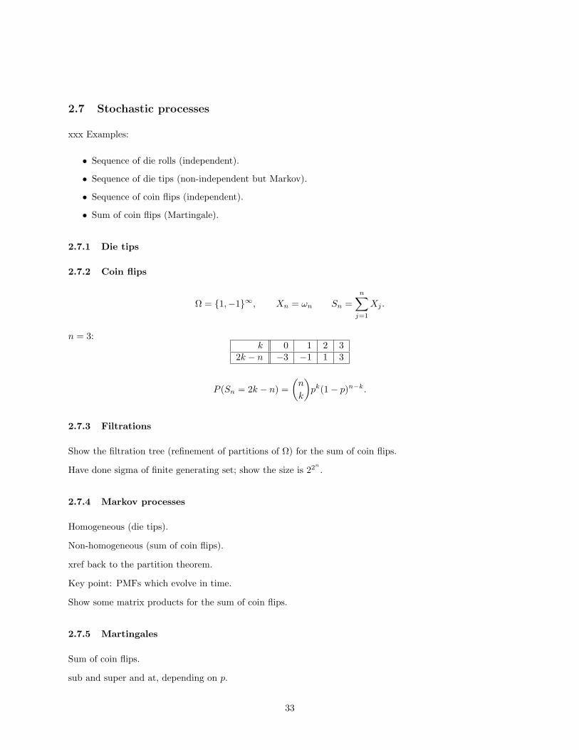
Ω = 1,−1∞, Xn = ωn Sn =n∑j=1
Xj .
n = 3:k 0 1 2 3
2k − n −3 −1 1 3
P (Sn = 2k − n) =(n
k
)pk(1− p)n−k.
2.7.3 Filtrations
Show the filtration tree (refinement of partitions of Ω) for the sum of coin flips.
Have done sigma of finite generating set; show the size is 22n
.
2.7.4 Markov processes
Homogeneous (die tips).
Non-homogeneous (sum of coin flips).
xref back to the partition theorem.
Key point: PMFs which evolve in time.
Show some matrix products for the sum of coin flips.
2.7.5 Martingales
Sum of coin flips.
sub and super and at, depending on p.
33
3 Statistics
The key concept here is parameter estimation. My goals are:
• Present a few concepts from parametric statistics, with an example-heavy approach.
• Give unified notation for probability and statistics.
• Work out several parameter-estimation examples concretely.
3.1 Sampling
3.1.1 Finite-population example
Work out an example with finite population x1, . . . , xn and simple random sample with replacementX1, . . . , XN.
Define µ and σ2.
Define unbiased estimator.
Show that X and s2 are unbiased estimators of µ and σ2 respectively. Explain the factor of n− 1 in s2.
3.1.2 Infinite-population example
3.2 Decision theory
The presentation here follows [Bha]. I am simply tabulating and elaborating upon his definitions.
One has the following:
• A population space Ω.
• An observation space or sample space X = Ωn containing observations X = (X1, . . . , Xn) whichare n-tuples of IID random variables on Ω.
• A parameter space Θ indexing (for θ ∈ Θ) a family of probability measures Pθ on (Ω,F). Then foreach Pθ one obtains a probability space (Ω,F , Pθ). One can think of these measures Pθ as conditionalprobabilities P (x | θ).Nominally, Θ is Rd or some subset thereof.
• An action space A indexing (for θ ∈ Θ) a family of probability measures Pθ on (Ω,F).
Nominally, A is all or part of Θ. This is best explained by example: Suppose θ = (µ, σ2) where eachθ is a 2-tuple defining a normal probability distribution on the real line. Then one might want to useone’s observation only to estimate µ. Then Θ = R× R+ whereas A is merely R.
• The population space, sample space, parameter space, and action space are all measurable spaces withtheir respective σ-algebras.
34
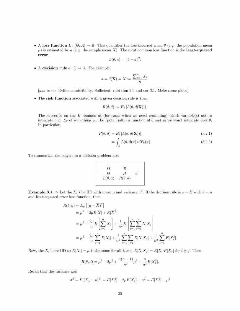
• A loss function L : (Θ,A)→ R. This quantifies the loss incurred when θ (e.g. the population meanµ) is estimated by a (e.g. the sample mean X). The most common loss function is the least-squarederror
L(θ, a) = ‖θ − a‖2.
• A decision rule d : X→ A. For example,
a = d(X) = X :=∑ni=1Xi
n.
[xxx to do: Define admissibility. Sufficient: rabi thm 3.3 and cor 3.1. Make some plots.]
• The risk function associated with a given decision rule is then
R(θ, d) := Eθ [L(θ, d(X))] .
The subscript on the E reminds us (for cases when we need reminding) which variable(s) not tointegrate out: Eθ of something will be (potentially) a function of θ and so we won’t integrate over θ.In particular,
R(θ, d) = Eθ [L(θ, d(X))] (3.2.1)
=∫
X
L(θ, d(x)) dPθ(x). (3.2.2)
To summarize, the players in a decision problem are:
Ω XΘ A d
L(θ, a) R(θ, d)
Example 3.1. B Let the Xi’s be IID with mean µ and variance σ2. If the decision rule is a = X with θ = µand least-squared-error loss function, then
R(θ, d) = Eµ[(µ−X)2
]= µ2 − 2µE[X] + E[X
2]
= µ2 − 2µnE
[n∑i=1
Xi
]+
1n2E
n∑i=1
n∑j=1
XiXj
= µ2 − 2µ
n
n∑i=1
E[Xi] +1n2
n∑i=1
∑j 6=i
E[XiXj ] +1n2
n∑i=1
E[X2i ].
Now, the Xi’s are IID so E[Xi] = µ is the same for all i, and E[XiXj ] = E[Xi]E[Xj ] for i 6= j. Then
R(θ, d) = µ2 − 2µ2 +n(n− 1)
n2µ2 +
n
n2E[X2
1 ].
Recall that the variance was
σ2 = E[(X1 − µ)2] = E[X21 ]− 2µE[X1] + µ2 = E[X2
1 ]− µ2
35
so
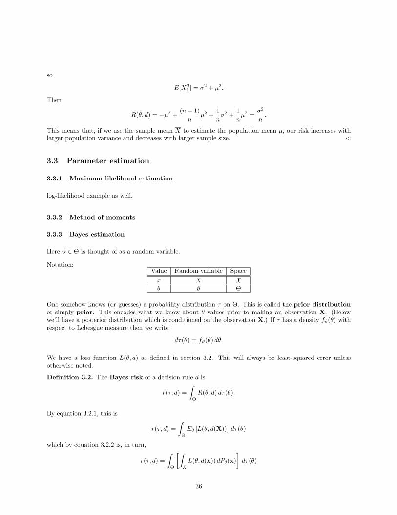
E[X21 ] = σ2 + µ2.
Then
R(θ, d) = −µ2 +(n− 1)n
µ2 +1nσ2 +
1nµ2 =
σ2
n.
This means that, if we use the sample mean X to estimate the population mean µ, our risk increases withlarger population variance and decreases with larger sample size. C
3.3 Parameter estimation
3.3.1 Maximum-likelihood estimation
log-likelihood example as well.
3.3.2 Method of moments
3.3.3 Bayes estimation
Here ϑ ∈ Θ is thought of as a random variable.
Notation:Value Random variable Spacex X X
θ ϑ Θ
One somehow knows (or guesses) a probability distribution τ on Θ. This is called the prior distributionor simply prior. This encodes what we know about θ values prior to making an observation X. (Belowwe’ll have a posterior distribution which is conditioned on the observation X.) If τ has a density fϑ(θ) withrespect to Lebesgue measure then we write
dτ(θ) = fϑ(θ) dθ.
We have a loss function L(θ, a) as defined in section 3.2. This will always be least-squared error unlessotherwise noted.
Definition 3.2. The Bayes risk of a decision rule d is
r(τ, d) =∫
Θ
R(θ, d) dτ(θ).
By equation 3.2.1, this is
r(τ, d) =∫
Θ
Eθ [L(θ, d(X))] dτ(θ)
which by equation 3.2.2 is, in turn,
r(τ, d) =∫
Θ
[∫X
L(θ, d(x)) dPθ(x)]dτ(θ)
36
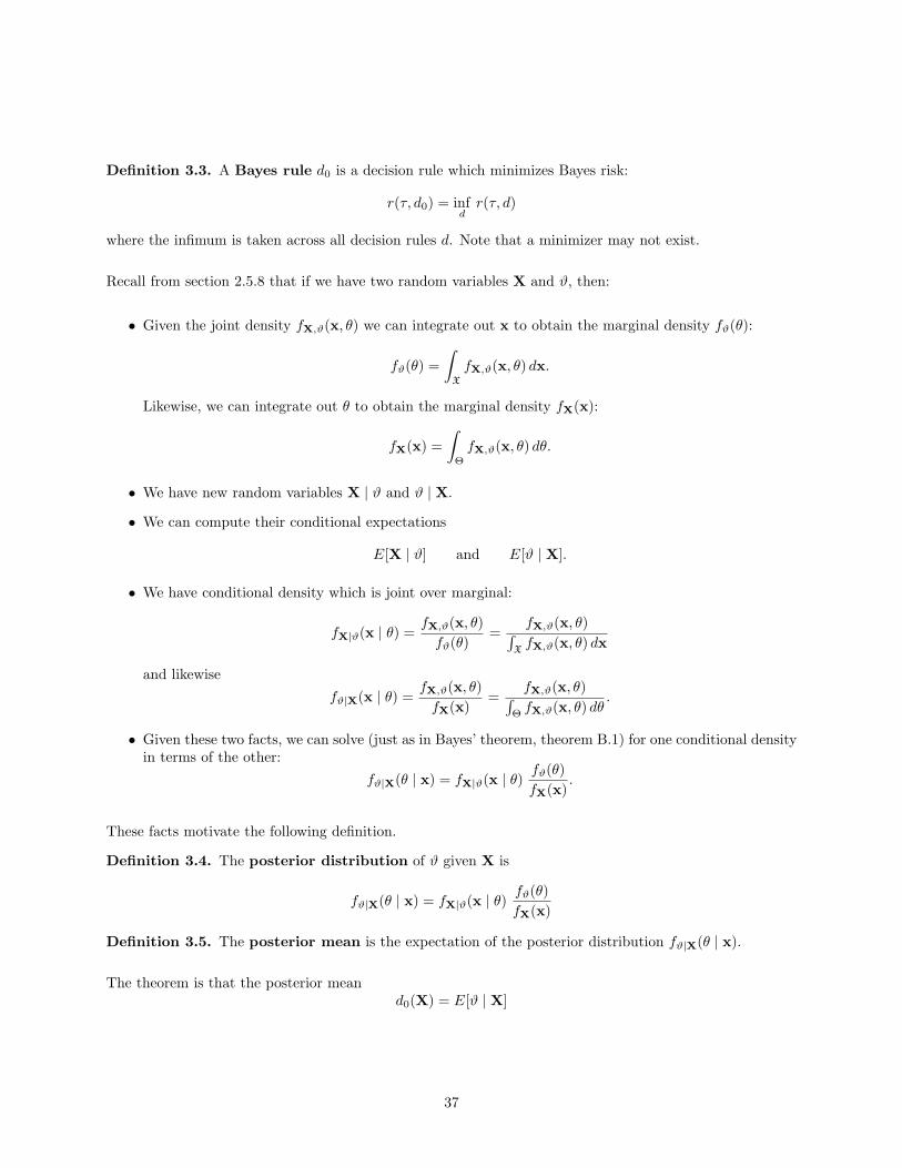
Definition 3.3. A Bayes rule d0 is a decision rule which minimizes Bayes risk:
r(τ, d0) = infdr(τ, d)
where the infimum is taken across all decision rules d. Note that a minimizer may not exist.
Recall from section 2.5.8 that if we have two random variables X and ϑ, then:
• Given the joint density fX,ϑ(x, θ) we can integrate out x to obtain the marginal density fϑ(θ):
fϑ(θ) =∫
X
fX,ϑ(x, θ) dx.
Likewise, we can integrate out θ to obtain the marginal density fX(x):
fX(x) =∫
Θ
fX,ϑ(x, θ) dθ.
• We have new random variables X | ϑ and ϑ | X.
• We can compute their conditional expectations
E[X | ϑ] and E[ϑ | X].
• We have conditional density which is joint over marginal:
fX|ϑ(x | θ) =fX,ϑ(x, θ)fϑ(θ)
=fX,ϑ(x, θ)∫
XfX,ϑ(x, θ) dx
and likewise
fϑ|X(x | θ) =fX,ϑ(x, θ)fX(x)
=fX,ϑ(x, θ)∫
ΘfX,ϑ(x, θ) dθ
.
• Given these two facts, we can solve (just as in Bayes’ theorem, theorem B.1) for one conditional densityin terms of the other:
fϑ|X(θ | x) = fX|ϑ(x | θ) fϑ(θ)fX(x)
.
These facts motivate the following definition.
Definition 3.4. The posterior distribution of ϑ given X is
fϑ|X(θ | x) = fX|ϑ(x | θ) fϑ(θ)fX(x)
Definition 3.5. The posterior mean is the expectation of the posterior distribution fϑ|X(θ | x).
The theorem is that the posterior meand0(X) = E[ϑ | X]
37
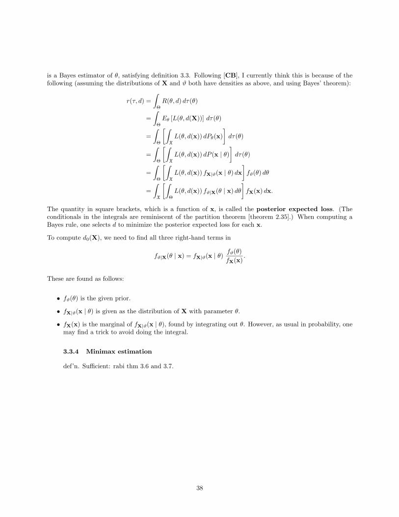
is a Bayes estimator of θ, satisfying definition 3.3. Following [CB], I currently think this is because of thefollowing (assuming the distributions of X and ϑ both have densities as above, and using Bayes’ theorem):
r(τ, d) =∫
Θ
R(θ, d) dτ(θ)
=∫
Θ
Eθ [L(θ, d(X))] dτ(θ)
=∫
Θ
[∫X
L(θ, d(x)) dPθ(x)]dτ(θ)
=∫
Θ
[∫X
L(θ, d(x)) dP (x | θ)]dτ(θ)
=∫
Θ
[∫X
L(θ, d(x)) fX|ϑ(x | θ) dx]fϑ(θ) dθ
=∫
X
[∫Θ
L(θ, d(x)) fϑ|X(θ | x) dθ]fX(x) dx.
The quantity in square brackets, which is a function of x, is called the posterior expected loss. (Theconditionals in the integrals are reminiscent of the partition theorem [theorem 2.35].) When computing aBayes rule, one selects d to minimize the posterior expected loss for each x.
To compute d0(X), we need to find all three right-hand terms in
fϑ|X(θ | x) = fX|ϑ(x | θ) fϑ(θ)fX(x)
.
These are found as follows:
• fϑ(θ) is the given prior.
• fX|ϑ(x | θ) is given as the distribution of X with parameter θ.
• fX(x) is the marginal of fX|ϑ(x | θ), found by integrating out θ. However, as usual in probability, onemay find a trick to avoid doing the integral.
3.3.4 Minimax estimation
def’n. Sufficient: rabi thm 3.6 and 3.7.
38
A The coin-flipping experiments
This section is an extended worked example, tying together various concepts. We apply the Central LimitTheorem first to repeated tosses of a single coin, then to repeated collections of tosses.
A.1 Single coin flips
The first experiment is tossing a single coin which has probability p of heads. Then Ω = T,H. Let X bethe random variable which takes value 0 for tails and 1 for heads. As discussed in section 2.2.2, X has theBernoulli distribution with parameter p. I will allow p to vary throughout this section, although I will focuson p = 0.5 and p = 0.6. Recall that X has mean
µX = p.
(In section 2.2.2 we took 1 for tails which is the opposite convention from the one here.) Its standarddeviation is
σX =√p(1− p),
which is√
0.25 = 0.5 and√
0.24 ≈ 0.4899 for p = 0.5 and p = 0.6, respectively.
Now flip the coin a large number n of times — say, n = 1000 — and count the number of heads. Using thenotation of section 2.5.4, the number of heads is Sn. There are two ways to look at this.
• On one hand, from section 2.2.2 we know that Sn is geometric with parameters p and n — if we thinkof the 1000 tosses as a single experiment. (This is precisely what we will do in the next section.) ThePMF of Sn is the one involving binomial coefficients; we would expect
µSn= np
i.e. 500 or 600 andσSn =
√np(1− p)
which is√
250 ≈ 15.81 or 240 ≈ 15.49 for p = 0.5 and p = 0.6, respectively.
• On the other hand, the Central Limit Theorem (section 2.6.3) says that as n increases, the distributionof Sn begins to look normal. This PDF involves the exponential function, as shown in section 2.5.4.The mean of the sums Sn is
µSn≈ nµX = np
(again 500 or 600). The standard deviation of those sums about the means 500 or 600 is
σSn ≈√nσX =
√np(1− p)
which are again 15.81 and 15.49, respectively.
Note that the binomial PMF and the normal PDF are not the same, even though they produced the samemeans and standard deviations: the geometric random variable has an integer-valued PMF; P (499.1 ≤ Sn ≤499.9) = 0 and likewise Sn can never be anything out of the range from 0 to 1000. The normal PDF, onthe other hand, gives P (499.1 ≤ Sn ≤ 499.9) 6= 0 since we are taking area under a curve where the functionis non-negative. Since the output of the exponential function is never 0, the normal PDF gives non-zero(although admittedly very, very tiny) probability of Sn being less than 0 or greater than 1000. (See also[MM] for some very nice plots.)
39
Now we can ask about fairness of coins. The probabilistic point of view is to fix p and ask about theprobabilities of various values of Sn. If the coin is fair, what are my chances of flipping anywhere between470 and 530 heads? Using the geometric PMF is a mess — in fact, my calculator can’t compute
(1000470
)without overflow. Using the normal approximation, though, is easy. I asked my TI-83 to integrate itsnormalpdf function, with µ = 500 and σ = 15.81, from 470 to 530 and it told me 0.9422.
How surprised should I be if I toss 580 heads? The standardization, which [MM] call the z-score, of Sn is(definition 2.123)
z =Sn − µSn
σSn
.
This counts how many standard deviations away from the mean a given observation is. I have 80/15.81 ≈ 5.06so this result is more than five standard deviations away from the mean. I would not think the coin is fair.If I re-do that computation with p = 0.6, µSn
= 600, and σSn= 15.49, I get a z-score of −1.29 which is not
surprising if the coin has parameter p = 0.6.
The point of view used in statistics is to start with the data, and from that try to estimate with variouslevels of confidence what the parameters are. Given a suspicious coin, what experiments would we have torun to be 95% sure that we’ve find out what the coin’s parameter p is, to within, say, ±0.01? Continuingthe example from section 2.6.4, we ask for ε = 0.01. We had
ε =1.96σX√
n
so, setting ε = 0.01 and solving for n, we have
n =(
1.96σX0.01
)2
=
(1.96
√p(1− p)
0.01
)2
≈ 38416 p(1− p).
Now, p(1 − p) has a maximum at p = 0.5, for which n = 9604, so that many flips would determine p towithin ±0.01 with 95% confidence. Re-doing the arithmetic with 0.001 in place of 0.01 gives n = 960, 400.Generalizing, we see that each additional decimal place costs 100 times as many runs.
A.2 Batches of coin flips
The second experiment is 1000 tosses of a coin where each coin has probability p of heads. (Or, think ofsimultaneously tossing 1000 identical such coins.) Then #Ω = 21000 ≈ 10301. Let Y : Ω→ R be the randomvariable which counts the number of heads. This is an example where the random variable is far easier todeal with than the entire sample space (which is huge).
As discussed in section 2.2.2, Y has the binomial distribution with parameters p and n = 1000. Recall fromthe previous section that that Y has mean
µY = 1000p,
e.g. 500 or 600. Likewise, its standard deviation is
σY =√
1000p(1− p),
which is√
250 ≈ 15.81 or 240 ≈ 15.49 for p = 0.5 and p = 0.6, respectively.
Let Y N be the average of N runs of this experiment — that is, the sample mean. The Central LimitTheorem (section 2.6.3) says that as N increases, the distribution of Y N begins to look normal. The meanof the sample means is
µY N≈ µY = 1000p,
40
which is again 500 or 600. The standard deviation of the sample means is
σY N≈ σY√
N=
√np(1− p)N
.
This is 15.81/√N or 15.49/
√N , respectively.
Here is the (crucial) interpretation: Given the parameters p and n of Y , there is a true population meanand a true population standard deviation. If p = 0.5, then σY ≈ 15.81 and even if we’re on the threemillionth iteration of the flip-1000-coins experiment, it’s still going to be quite likely as ever that we’ll geta 514 or a 492 and so on. If we don’t know the true p of the coins then, while the true population meanµY and the true population standard deviation σY exist, we don’t know what they are. All we have is somesuspicious-looking identical coins and our laboratory equipment. As we run and re-run the flip-1000-coinsexperiment, the following happens:
• The sample mean µY N, for increasingly larger N , will approach the population mean µY .
• The variations of the sample mean will decrease. We might say the error in our estimate of thepopulation mean is shrinking.
• The population standard deviation appears in the above formulas via its effects on the standard devi-ation of the sample mean.
• Nothing we have done so far has given us a reliable connection between the sample standard deviationand the population standard deviation. We can guess that the sample standard deviation approachesthe population standard deviation, but (in this course) we have not developed any information aboutthe error in that computation.
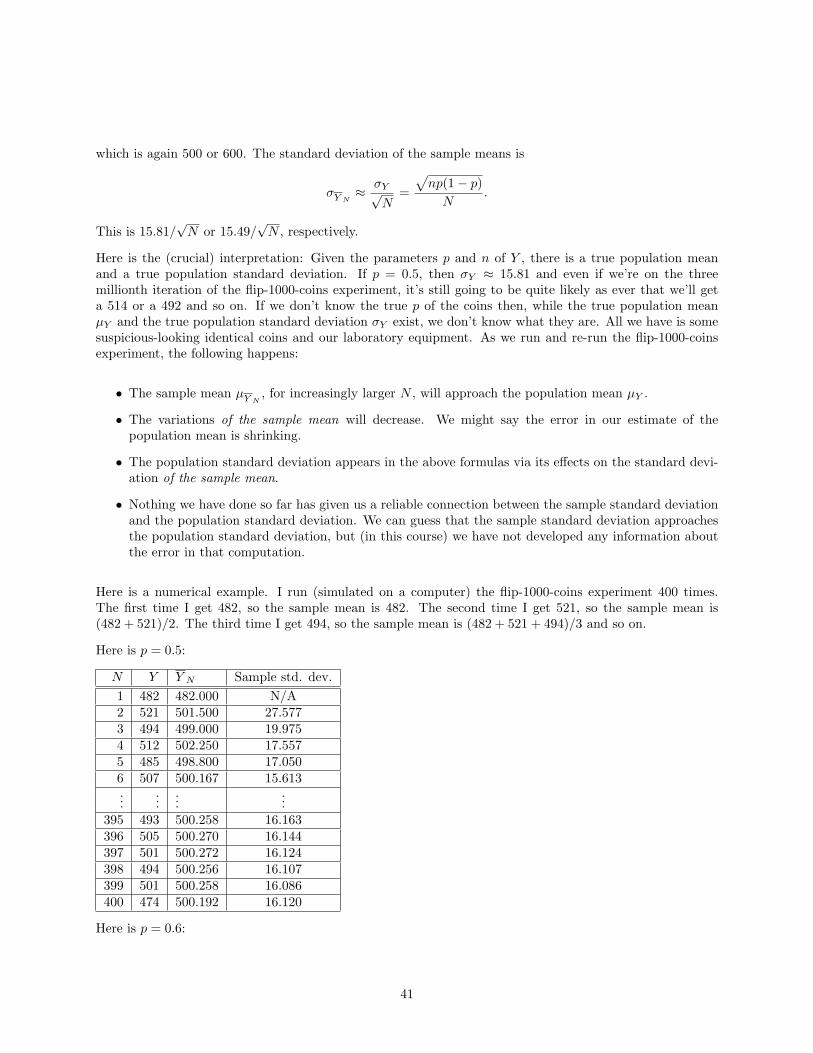
Here is a numerical example. I run (simulated on a computer) the flip-1000-coins experiment 400 times.The first time I get 482, so the sample mean is 482. The second time I get 521, so the sample mean is(482 + 521)/2. The third time I get 494, so the sample mean is (482 + 521 + 494)/3 and so on.
Here is p = 0.5:
N Y Y N Sample std. dev.1 482 482.000 N/A2 521 501.500 27.5773 494 499.000 19.9754 512 502.250 17.5575 485 498.800 17.0506 507 500.167 15.613...
......
...395 493 500.258 16.163396 505 500.270 16.144397 501 500.272 16.124398 494 500.256 16.107399 501 500.258 16.086400 474 500.192 16.120
Here is p = 0.6:
41

N Y Y N Sample std. dev.1 616 616.000 N/A2 584 600.000 22.6273 620 606.667 19.7324 617 609.250 16.9195 583 604.000 18.7756 613 605.500 17.190...
......
...395 608 599.484 17.031396 615 599.523 17.027397 609 599.547 17.013398 607 599.565 16.995399 604 599.576 16.975400 611 599.605 16.964
42
B Bayes’ theorem
Bayes’ theorem is so important that it merits multiple points of view: algebraic, graphical, and numerical.
B.1 Algebraic approach
Recall from definition 2.12 that if A is an event, and if B is another event with non-zero probability, theconditional probability of A given B is
P (A|B) =P (A ∩B)P (B)
.
Bayes’ theorem tells us how to invert this: how to compute the probability of B given A. First, the algebraictreatment.
Theorem B.1 (Bayes’ theorem). Let A and B be events with non-zero probability. Then
P (B|A) = P (A|B)P (B)P (A)
.
Proof. Using the definition (intersection over given), we have
P (B|A) =P (B ∩A)P (A)
.
Multiplying top and bottom by P (B) (which is OK since P (B) 6= 0) we get
P (B|A) =P (B ∩A)P (A)
P (B)P (B)
.
Now notice that B∩A is the same as A∩B, so in particular P (B∩A) is the same as P (A∩B). Transposingthe terms in the denominator gives us
P (B|A) =P (A ∩B)P (B)
P (B)P (A)
= P (A|B)P (B)P (A)
as desired.
B.2 Graphical/numerical approach
The following example is adapted from [KK]. Suppose that 0.8% of the general population has a certaindisease, and suppose that we have a test for it. Specifically, if a person actually has the disease, the test saysso 90% of the time. If a person does not have the disease, the test gives a false diagnosis 7% of the time.When a particular patient tests positive, what is the probability they have the disease?
We can write this symbolically as follows. Let D be the event that the person has the disease and D be itscomplement; let Y (for “yes”) be the event that the test says the person has the disease, with complement
43
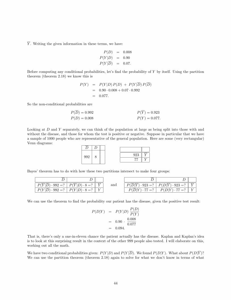
Y . Writing the given information in these terms, we have:
P (D) = 0.008P (Y |D) = 0.90P (Y |D) = 0.07.
Before computing any conditional probabilities, let’s find the probability of Y by itself. Using the partitiontheorem (theorem 2.18) we know this is
P (Y ) = P (Y |D)P (D) + P (Y |D)P (D)= 0.90 · 0.008 + 0.07 · 0.992= 0.077.
So the non-conditional probabilities are
P (D) = 0.992 P (Y ) = 0.923P (D) = 0.008 P (Y ) = 0.077.
Looking at D and Y separately, we can think of the population at large as being split into those with andwithout the disease, and those for whom the test is positive or negative. Suppose in particular that we havea sample of 1000 people who are representative of the general population. Here are some (very rectangular)Venn diagrams:
D D
992 8 923 Y77 Y
Bayes’ theorem has to do with how these two partitions intersect to make four groups:
D D
P (Y |D) · 992 =? P (Y |D) · 8 =? Y
P (Y |D) · 992 =? P (Y |D) · 8 =? Y
andD D
P (D|Y ) · 923 =? P (D|Y ) · 923 =? Y
P (D|Y ) · 77 =? P (D|Y ) · 77 =? Y
We can use the theorem to find the probability our patient has the disease, given the positive test result:
P (D|Y ) = P (Y |D)P (D)P (Y )
= 0.90 · 0.0080.077
= 0.094.
That is, there’s only a one-in-eleven chance the patient actually has the disease. Kaplan and Kaplan’s ideais to look at this surprising result in the context of the other 999 people also tested. I will elaborate on this,working out all the math.
We have two conditional probabilities given: P (Y |D) and P (Y |D). We found P (D|Y ). What about P (D|Y )?We can use the partition theorem (theorem 2.18) again to solve for what we don’t know in terms of what
44

we do know:
P (D) = P (D|Y )P (Y ) + P (D|Y )P (Y )
P (D|Y ) =P (D)− P (D|Y )P (Y )
P (Y )
=0.008− 0.094 · 0.077
0.923= 0.0008.
We now have all four conditional probabilities:
P (Y |D) = 0.07 P (D|Y ) = 0.0008P (Y |D) = 0.90 P (D|Y ) = 0.094.
Now we can fill out the four-square table:
• Since P (Y |D) = 0.07, seven percent of the 992 disease-free people (70 of them) get false positives; therest (922) get a correct negative result.
• Since P (Y |D) = 0.90, ninety percent of the 8 people with the disease test positive (i.e. all but one ofthem); one of the 8 gets a false sense of security.
• Since P (D|Y ) = 0.0008, 0.08% of the 923 with negative test results (one person) does in fact have thedisease; the other 922 (as we found just above) get a correct negative result.
• Since P (D|Y ) = 0.094, only 9.4% of the 77 people with positive test results (7 people) have the disease;the other 70 get a scare (and, presumably, a re-test).
So, the sample of 1000 people splits up as follows:
D D
922 1 Y70 7 Y
Moreover, we can rank events by likelihood:
(1) Healthy people correctly diagnosed: 92.2%.
(2) False positives: 7%.
(3) People with the disease, correctly diagnosed: 0.7%.
(4) False negatives: 0.1%.
Now it’s no surprise our patient got a false positive: this happens 10 times as often as a correct positivediagnosis.
B.3 Asymptotics
The specific example provided some insight, but what happens when we vary the parameters? We had
P (D|Y ) =P (Y |D)P (D)
P (Y )=
P (Y |D)P (D)P (Y |D)P (D) + P (Y |D)P (D)
.
45
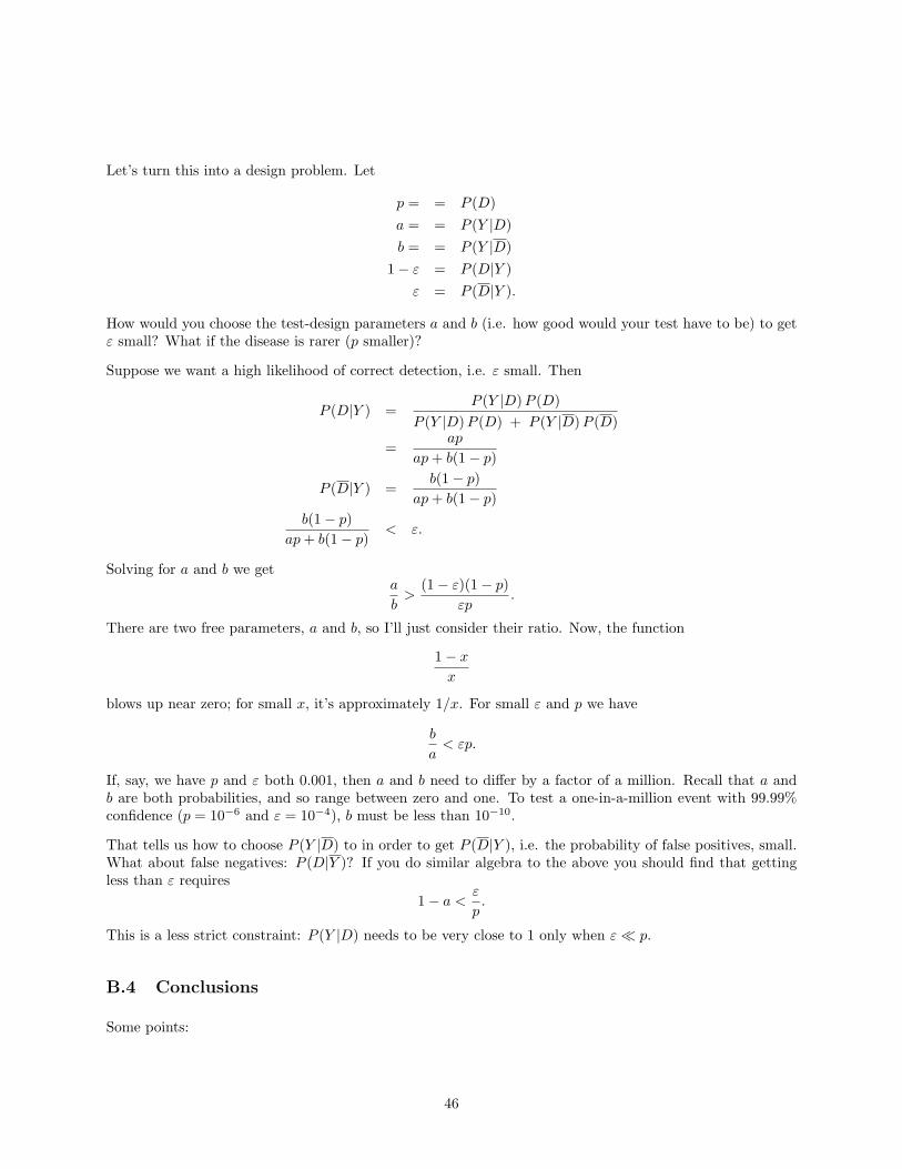
Let’s turn this into a design problem. Let
p = = P (D)a = = P (Y |D)b = = P (Y |D)
1− ε = P (D|Y )ε = P (D|Y ).
How would you choose the test-design parameters a and b (i.e. how good would your test have to be) to getε small? What if the disease is rarer (p smaller)?
Suppose we want a high likelihood of correct detection, i.e. ε small. Then
P (D|Y ) =P (Y |D)P (D)
P (Y |D)P (D) + P (Y |D)P (D)
=ap
ap+ b(1− p)
P (D|Y ) =b(1− p)
ap+ b(1− p)b(1− p)
ap+ b(1− p)< ε.
Solving for a and b we geta
b>
(1− ε)(1− p)εp
.
There are two free parameters, a and b, so I’ll just consider their ratio. Now, the function
1− xx
blows up near zero; for small x, it’s approximately 1/x. For small ε and p we have
b
a< εp.
If, say, we have p and ε both 0.001, then a and b need to differ by a factor of a million. Recall that a andb are both probabilities, and so range between zero and one. To test a one-in-a-million event with 99.99%confidence (p = 10−6 and ε = 10−4), b must be less than 10−10.
That tells us how to choose P (Y |D) to in order to get P (D|Y ), i.e. the probability of false positives, small.What about false negatives: P (D|Y )? If you do similar algebra to the above you should find that gettingless than ε requires
1− a < ε
p.
This is a less strict constraint: P (Y |D) needs to be very close to 1 only when ε p.
B.4 Conclusions
Some points:
46
• P (Y |D) is information known to the person who creates the test — say, at a pharmaceutical company;P (D|Y ) is information relevant to the people who give and receive the test — for example, at thedoctor’s office. This duality between design and implementation suggests that Bayes’ theorem hasimportant consequences in many practical situations.
• The results can be surprising — after all, in the example above the test was 90% accurate, was it not?Bayes’ theorem is important to know precisely because it is counterintuitive.
• We can see from the example and the asymptotics above that rare events are hard to test accuratelyfor. If we want certain testing for rare events, the test might be impossible (or overly expensive) todesign in practical terms.
47
C Probability and measure theory
Probability theory is measure theory with a soul.— Mark Kac.
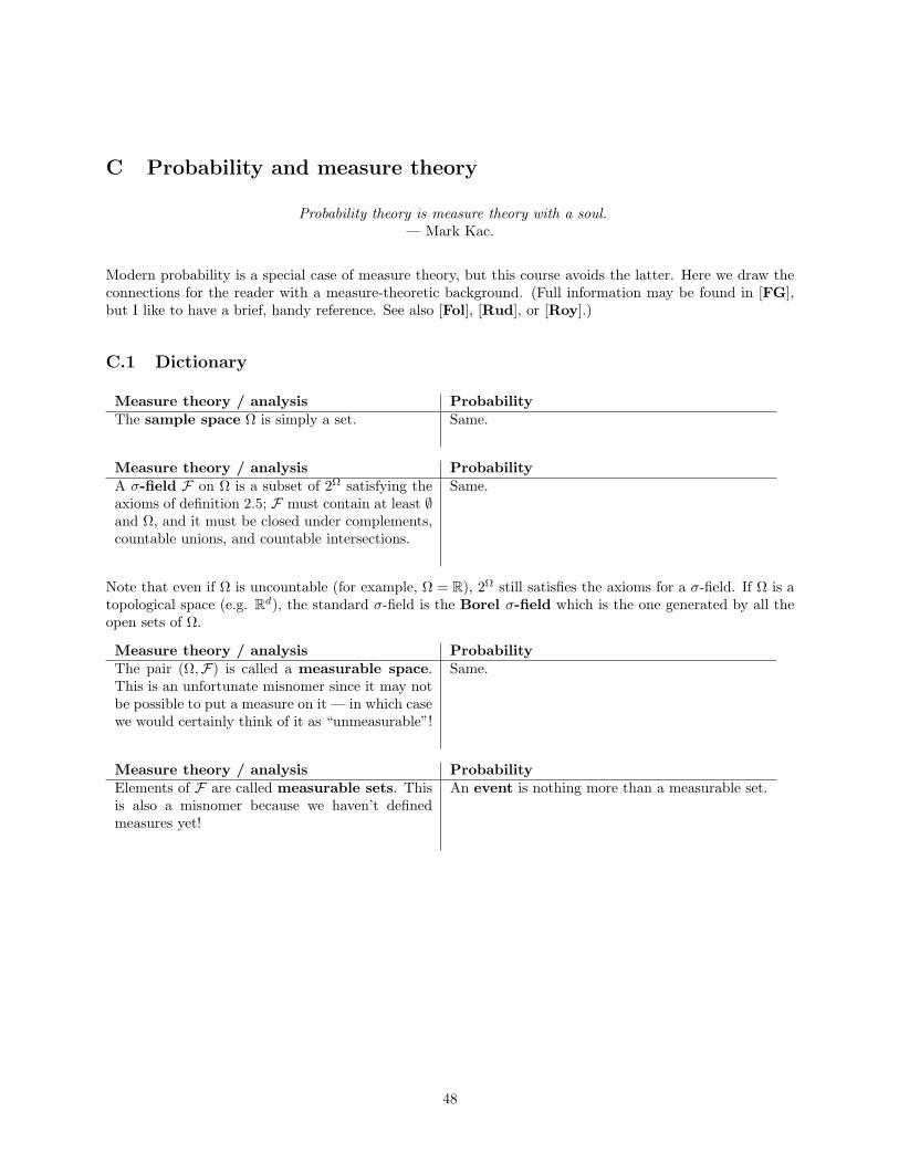
Modern probability is a special case of measure theory, but this course avoids the latter. Here we draw theconnections for the reader with a measure-theoretic background. (Full information may be found in [FG],but I like to have a brief, handy reference. See also [Fol], [Rud], or [Roy].)
C.1 Dictionary
Measure theory / analysis ProbabilityThe sample space Ω is simply a set. Same.
Measure theory / analysis ProbabilityA σ-field F on Ω is a subset of 2Ω satisfying theaxioms of definition 2.5; F must contain at least ∅and Ω, and it must be closed under complements,countable unions, and countable intersections.
Same.
Note that even if Ω is uncountable (for example, Ω = R), 2Ω still satisfies the axioms for a σ-field. If Ω is atopological space (e.g. Rd), the standard σ-field is the Borel σ-field which is the one generated by all theopen sets of Ω.
Measure theory / analysis ProbabilityThe pair (Ω,F) is called a measurable space.This is an unfortunate misnomer since it may notbe possible to put a measure on it — in which casewe would certainly think of it as “unmeasurable”!
Same.
Measure theory / analysis ProbabilityElements of F are called measurable sets. Thisis also a misnomer because we haven’t definedmeasures yet!
An event is nothing more than a measurable set.
48
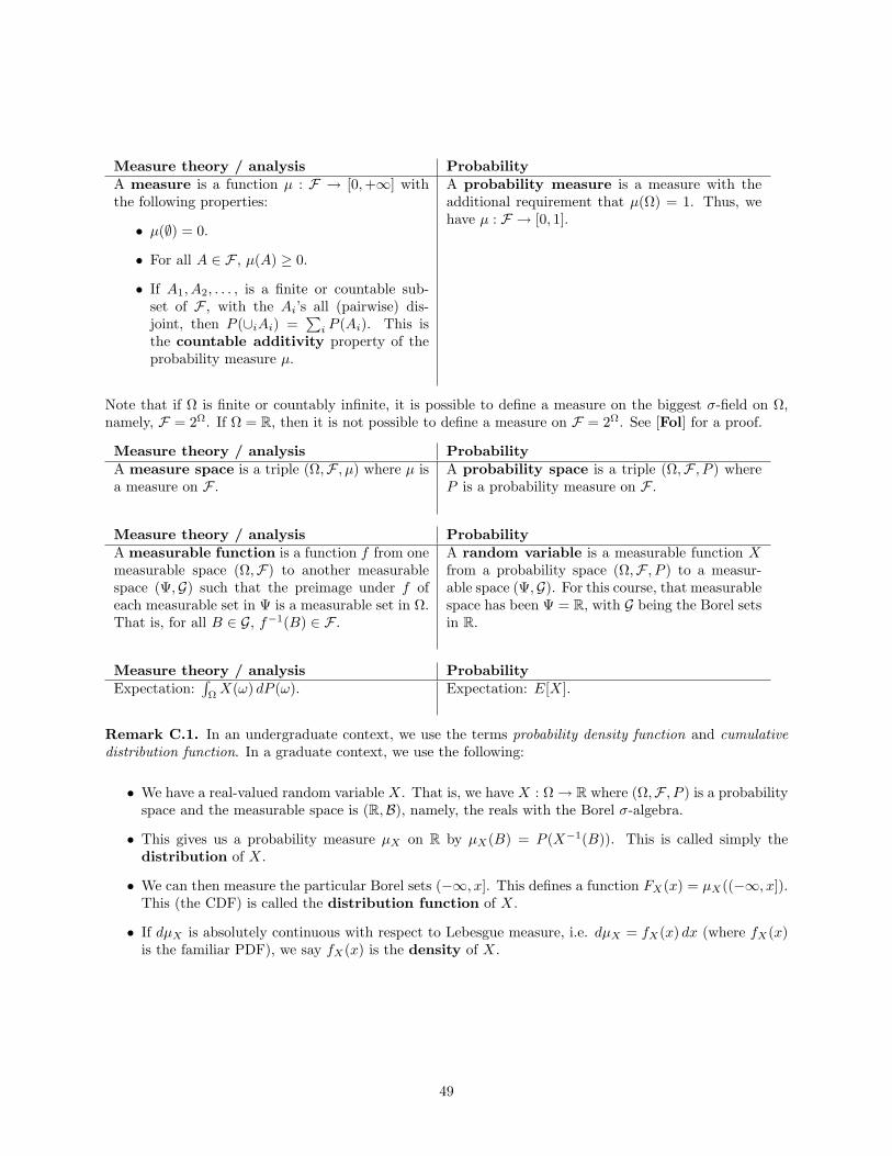
Measure theory / analysis ProbabilityA measure is a function µ : F → [0,+∞] withthe following properties:
• µ(∅) = 0.
• For all A ∈ F , µ(A) ≥ 0.
• If A1, A2, . . . , is a finite or countable sub-set of F , with the Ai’s all (pairwise) dis-joint, then P (∪iAi) =
∑i P (Ai). This is
the countable additivity property of theprobability measure µ.
A probability measure is a measure with theadditional requirement that µ(Ω) = 1. Thus, wehave µ : F → [0, 1].
Note that if Ω is finite or countably infinite, it is possible to define a measure on the biggest σ-field on Ω,namely, F = 2Ω. If Ω = R, then it is not possible to define a measure on F = 2Ω. See [Fol] for a proof.
Measure theory / analysis ProbabilityA measure space is a triple (Ω,F , µ) where µ isa measure on F .
A probability space is a triple (Ω,F , P ) whereP is a probability measure on F .
Measure theory / analysis ProbabilityA measurable function is a function f from onemeasurable space (Ω,F) to another measurablespace (Ψ,G) such that the preimage under f ofeach measurable set in Ψ is a measurable set in Ω.That is, for all B ∈ G, f−1(B) ∈ F .
A random variable is a measurable function Xfrom a probability space (Ω,F , P ) to a measur-able space (Ψ,G). For this course, that measurablespace has been Ψ = R, with G being the Borel setsin R.
Measure theory / analysis ProbabilityExpectation:
∫ΩX(ω) dP (ω). Expectation: E[X].
Remark C.1. In an undergraduate context, we use the terms probability density function and cumulativedistribution function. In a graduate context, we use the following:
• We have a real-valued random variable X. That is, we have X : Ω→ R where (Ω,F , P ) is a probabilityspace and the measurable space is (R,B), namely, the reals with the Borel σ-algebra.
• This gives us a probability measure µX on R by µX(B) = P (X−1(B)). This is called simply thedistribution of X.
• We can then measure the particular Borel sets (−∞, x]. This defines a function FX(x) = µX((−∞, x]).This (the CDF) is called the distribution function of X.
• If dµX is absolutely continuous with respect to Lebesgue measure, i.e. dµX = fX(x) dx (where fX(x)is the familiar PDF), we say fX(x) is the density of X.
49
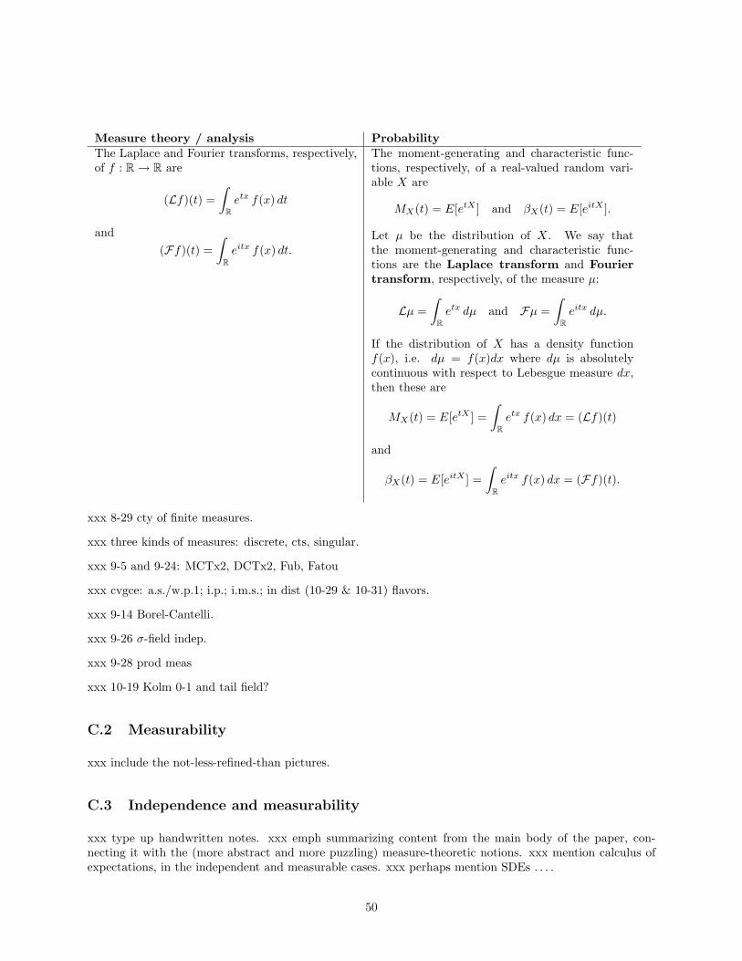
Measure theory / analysis ProbabilityThe Laplace and Fourier transforms, respectively,of f : R→ R are
(Lf)(t) =∫
Retx f(x) dt
and(Ff)(t) =
∫Reitx f(x) dt.
The moment-generating and characteristic func-tions, respectively, of a real-valued random vari-able X are
MX(t) = E[etX ] and βX(t) = E[eitX ].
Let µ be the distribution of X. We say thatthe moment-generating and characteristic func-tions are the Laplace transform and Fouriertransform, respectively, of the measure µ:
Lµ =∫
Retx dµ and Fµ =
∫Reitx dµ.
If the distribution of X has a density functionf(x), i.e. dµ = f(x)dx where dµ is absolutelycontinuous with respect to Lebesgue measure dx,then these are
MX(t) = E[etX ] =∫
Retx f(x) dx = (Lf)(t)
and
βX(t) = E[eitX ] =∫
Reitx f(x) dx = (Ff)(t).
xxx 8-29 cty of finite measures.
xxx three kinds of measures: discrete, cts, singular.
xxx 9-5 and 9-24: MCTx2, DCTx2, Fub, Fatou
xxx cvgce: a.s./w.p.1; i.p.; i.m.s.; in dist (10-29 & 10-31) flavors.
xxx 9-14 Borel-Cantelli.
xxx 9-26 σ-field indep.
xxx 9-28 prod meas
xxx 10-19 Kolm 0-1 and tail field?
C.2 Measurability
xxx include the not-less-refined-than pictures.
C.3 Independence and measurability
xxx type up handwritten notes. xxx emph summarizing content from the main body of the paper, con-necting it with the (more abstract and more puzzling) measure-theoretic notions. xxx mention calculus ofexpectations, in the independent and measurable cases. xxx perhaps mention SDEs . . . .
50
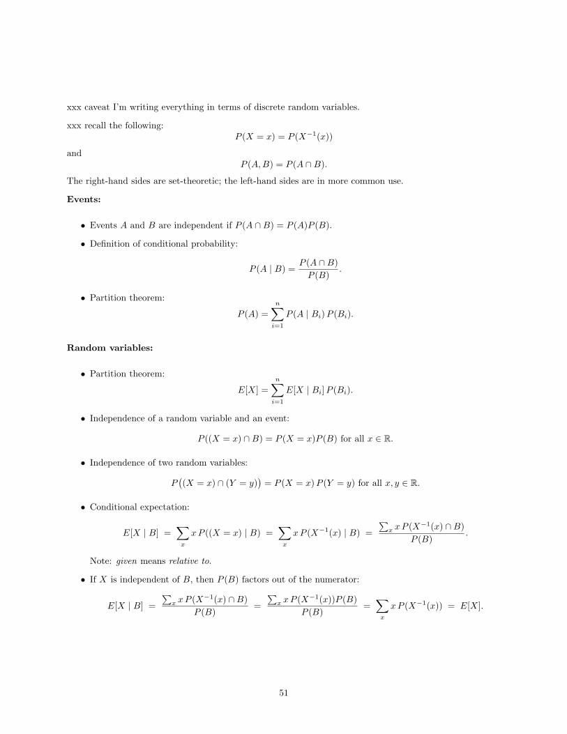
xxx caveat I’m writing everything in terms of discrete random variables.
xxx recall the following:P (X = x) = P (X−1(x))
andP (A,B) = P (A ∩B).
The right-hand sides are set-theoretic; the left-hand sides are in more common use.
Events:
• Events A and B are independent if P (A ∩B) = P (A)P (B).
• Definition of conditional probability:
P (A | B) =P (A ∩B)P (B)
.
• Partition theorem:
P (A) =n∑i=1
P (A | Bi)P (Bi).
Random variables:
• Partition theorem:
E[X] =n∑i=1
E[X | Bi]P (Bi).
• Independence of a random variable and an event:
P ((X = x) ∩B) = P (X = x)P (B) for all x ∈ R.
• Independence of two random variables:
P((X = x) ∩ (Y = y)
)= P (X = x)P (Y = y) for all x, y ∈ R.
• Conditional expectation:
E[X | B] =∑x
xP ((X = x) | B) =∑x
xP (X−1(x) | B) =∑x xP (X−1(x) ∩B)
P (B).
Note: given means relative to.
• If X is independent of B, then P (B) factors out of the numerator:
E[X | B] =∑x xP (X−1(x) ∩B)
P (B)=∑x xP (X−1(x))P (B)
P (B)=∑x
xP (X−1(x)) = E[X].
51
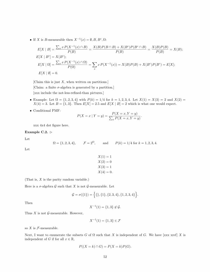
• If X is B-measurable then X−1(x) = ∅, B,Bc,Ω:
E[X | B] =∑x xP (X−1(x) ∩B)
P (B)=X(B)P (B ∩B) +X(Bc)P (Bc ∩B)
P (B)=X(B)P (B)P (B)
= X(B);
E[X | Bc] = X(Bc);
E[X | Ω] =∑x xP (X−1(x) ∩ Ω)
P (Ω)=∑x
xP (X−1(x)) = X(B)P (B) +X(Bc)P (Bc) = E[X];
E[X | ∅] = 0.
[Claim this is just X, when written on partitions.]
[Claim: a finite σ-algebra is generated by a partition.]
[xxx include the not-less-refined-than pictures.]
• Example: Let Ω = 1, 2, 3, 4 with P (k) = 1/4 for k = 1, 2, 3, 4. Let X(1) = X(3) = 2 and X(2) =X(4) = 3. Let B = 1, 3. Then E[X] = 2.5 and E[X | B] = 2 which is what one would expect.
• Conditional PMF:
P (X = x | Y = y) =P (X = x, Y = y)∑x P (X = x, Y = y)
.
xxx 4x4 dot figure here.
Example C.2. B
LetΩ = 1, 2, 3, 4, F = 2Ω, and P (k) = 1/4 for k = 1, 2, 3, 4.
Let
X(1) = 1X(2) = 0X(3) = 1X(4) = 0.
(That is, X is the parity random variable.)
Here is a σ-algebra G such that X is not G-measurable. Let
G = σ(1) =, 1, 2, 3, 4, 1, 2, 3, 4
.
ThenX−1(1) = 1, 3 6∈ G.
Thus X is not G-measurable. However,
X−1(1) = 1, 3 ∈ F
so X is F-measurable.
Next, I want to enumerate the subsets G of Ω such that X is independent of G. We have [xxx xref] X isindependent of G if for all x ∈ R,
P ((X = k) ∩G) = P (X = k)P (G).
52

For brevity (so that the table below will fit on the page), write
A0 = X−1(0) and A1 = X−1(1).
Ordered by sizes of G’s:
G A0 ∩G A1 ∩G P (G) P (A0)P (G) P (A0 ∩G) P (A1)P (G) P (A1 ∩G) Indep.? 0 0 0 0 0 yes1 1 1/4 1/8 0 1/8 1/4 no2 2 1/4 1/8 1/4 1/8 0 no3 3 1/4 1/8 0 1/8 1/4 no4 4 1/4 1/8 1/4 1/8 0 no1, 3 1, 3 1/2 1/4 0 1/4 1/2 no2, 4 2, 4 1/2 1/4 1/2 1/4 0 no1, 2 2 1 1/2 1/4 1/4 1/4 1/4 yes1, 4 4 1 1/2 1/4 1/4 1/4 1/4 yes2, 3 2 3 1/2 1/4 1/4 1/4 1/4 yes3, 4 4 3 1/2 1/4 1/4 1/4 1/4 yes1, 2, 3 2 1, 3 3/4 3/8 1/4 3/8 1/2 no1, 2, 4 2, 4 1 3/4 3/8 1/2 3/8 1/4 no1, 3, 4 4 1, 3 3/4 3/8 1/4 3/8 1/2 no2, 3, 4 2, 4 3 3/4 3/8 1/2 3/8 1/4 no1, 2, 3, 4 2, 4 1, 3 1 1/2 1/2 1/2 1/2 yes
Ordered by independence and dependence:
G A0 ∩G A1 ∩G P (G) P (A0)P (G) P (A0 ∩G) P (A1)P (G) P (A1 ∩G) Indep.? 0 0 0 0 0 yes1, 2 2 1 1/2 1/4 1/4 1/4 1/4 yes1, 4 4 1 1/2 1/4 1/4 1/4 1/4 yes2, 3 2 3 1/2 1/4 1/4 1/4 1/4 yes3, 4 4 3 1/2 1/4 1/4 1/4 1/4 yes1, 2, 3, 4 2, 4 1, 3 1 1/2 1/2 1/2 1/2 yes1 1 1/4 1/8 0 1/8 1/4 no2 2 1/4 1/8 1/4 1/8 0 no3 3 1/4 1/8 0 1/8 1/4 no4 4 1/4 1/8 1/4 1/8 0 no1, 3 1, 3 1/2 1/4 0 1/4 1/2 no2, 4 2, 4 1/2 1/4 1/2 1/4 0 no1, 2, 3 2 1, 3 3/4 3/8 1/4 3/8 1/2 no1, 2, 4 2, 4 1 3/4 3/8 1/2 3/8 1/4 no1, 3, 4 4 1, 3 3/4 3/8 1/4 3/8 1/2 no2, 3, 4 2, 4 3 3/4 3/8 1/2 3/8 1/4 no
C
53
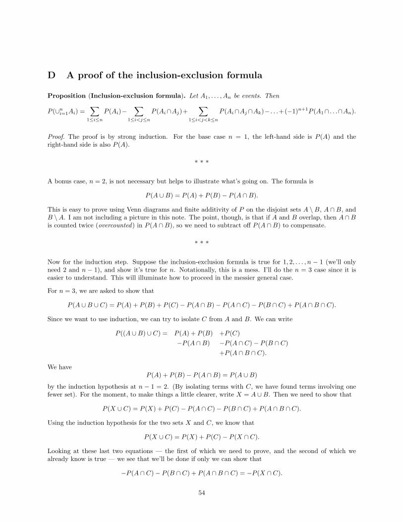
D A proof of the inclusion-exclusion formula
Proposition (Inclusion-exclusion formula). Let A1, . . . , An be events. Then
P (∪ni=1Ai) =∑
1≤i≤n
P (Ai)−∑
1≤i<j≤n
P (Ai∩Aj)+∑
1≤i<j<k≤n
P (Ai∩Aj∩Ak)− . . .+(−1)n+1P (A1∩ . . .∩An).
Proof. The proof is by strong induction. For the base case n = 1, the left-hand side is P (A) and theright-hand side is also P (A).
* * *
A bonus case, n = 2, is not necessary but helps to illustrate what’s going on. The formula is
P (A ∪B) = P (A) + P (B)− P (A ∩B).
This is easy to prove using Venn diagrams and finite additivity of P on the disjoint sets A \B, A ∩B, andB \A. I am not including a picture in this note. The point, though, is that if A and B overlap, then A ∩Bis counted twice (overcounted) in P (A ∩B), so we need to subtract off P (A ∩B) to compensate.
* * *
Now for the induction step. Suppose the inclusion-exclusion formula is true for 1, 2, . . . , n − 1 (we’ll onlyneed 2 and n − 1), and show it’s true for n. Notationally, this is a mess. I’ll do the n = 3 case since it iseasier to understand. This will illuminate how to proceed in the messier general case.
For n = 3, we are asked to show that
P (A ∪B ∪ C) = P (A) + P (B) + P (C)− P (A ∩B)− P (A ∩ C)− P (B ∩ C) + P (A ∩B ∩ C).
Since we want to use induction, we can try to isolate C from A and B. We can write
P ((A ∪B) ∪ C) = P (A) + P (B) +P (C)−P (A ∩B) −P (A ∩ C)− P (B ∩ C)
+P (A ∩B ∩ C).
We haveP (A) + P (B)− P (A ∩B) = P (A ∪B)
by the induction hypothesis at n − 1 = 2. (By isolating terms with C, we have found terms involving onefewer set). For the moment, to make things a little clearer, write X = A ∪B. Then we need to show that
P (X ∪ C) = P (X) + P (C)− P (A ∩ C)− P (B ∩ C) + P (A ∩B ∩ C).
Using the induction hypothesis for the two sets X and C, we know that
P (X ∪ C) = P (X) + P (C)− P (X ∩ C).
Looking at these last two equations — the first of which we need to prove, and the second of which wealready know is true — we see that we’ll be done if only we can show that
−P (A ∩ C)− P (B ∩ C) + P (A ∩B ∩ C) = −P (X ∩ C).
54
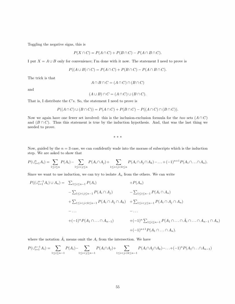
Toggling the negative signs, this is
P (X ∩ C) = P (A ∩ C) + P (B ∩ C)− P (A ∩B ∩ C).
I put X = A ∪B only for convenience; I’m done with it now. The statement I need to prove is
P ((A ∪B) ∩ C) = P (A ∩ C) + P (B ∩ C)− P (A ∩B ∩ C).
The trick is thatA ∩B ∩ C = (A ∩ C) ∩ (B ∩ C)
and(A ∪B) ∩ C = (A ∩ C) ∪ (B ∩ C).
That is, I distribute the C’s. So, the statement I need to prove is
P ((A ∩ C) ∪ (B ∩ C)) = P (A ∩ C) + P (B ∩ C)− P ((A ∩ C) ∩ (B ∩ C)).
Now we again have one fewer set involved: this is the inclusion-exclusion formula for the two sets (A ∩ C)and (B ∩ C). Thus this statement is true by the induction hypothesis. And, that was the last thing weneeded to prove.
* * *
Now, guided by the n = 3 case, we can confidently wade into the morass of subscripts which is the inductionstep. We are asked to show that
P (∪ni=1Ai) =∑
1≤i≤n
P (Ai)−∑
1≤i<j≤n
P (Ai∩Aj)+∑
1≤i<j<k≤n
P (Ai∩Aj∩Ak)− . . .+(−1)n+1P (A1∩ . . .∩An).
Since we want to use induction, we can try to isolate An from the others. We can write
P ((∪n−1i=1 Ai) ∪An) =
∑1≤i≤n−1 P (Ai) +P (An)
−∑
1≤i<j≤n−1 P (Ai ∩Aj) −∑
1≤i≤n−1 P (Ai ∩An)
+∑
1≤i<j<k≤n−1 P (Ai ∩Aj ∩Ak) +∑
1≤i<j≤n−1 P (Ai ∩Aj ∩An)
− . . . − . . .
+(−1)nP (A1 ∩ . . . ∩An−1) +(−1)n∑
1≤i≤n−1 P (A1 ∩ . . . ∩ Ai ∩ . . . ∩An−1 ∩An)
+(−1)n+1P (A1 ∩ . . . ∩An).
where the notation Ai means omit the Ai from the intersection. We have
P (∪n−1i=1 Ai) =
∑1≤i≤n−1
P (Ai)−∑
1≤i<j≤n−1
P (Ai∩Aj)+∑
1≤i<j<k≤n−1
P (Ai∩Aj∩Ak)−. . .+(−1)nP (A1∩. . .∩An−1)
55
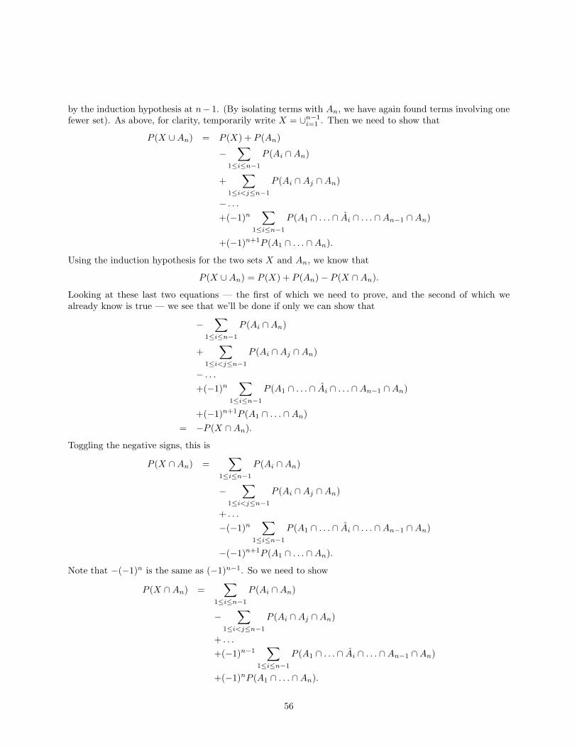
by the induction hypothesis at n− 1. (By isolating terms with An, we have again found terms involving onefewer set). As above, for clarity, temporarily write X = ∪n−1
i=1 . Then we need to show that
P (X ∪An) = P (X) + P (An)
−∑
1≤i≤n−1
P (Ai ∩An)
+∑
1≤i<j≤n−1
P (Ai ∩Aj ∩An)
− . . .+(−1)n
∑1≤i≤n−1
P (A1 ∩ . . . ∩ Ai ∩ . . . ∩An−1 ∩An)
+(−1)n+1P (A1 ∩ . . . ∩An).
Using the induction hypothesis for the two sets X and An, we know that
P (X ∪An) = P (X) + P (An)− P (X ∩An).
Looking at these last two equations — the first of which we need to prove, and the second of which wealready know is true — we see that we’ll be done if only we can show that
−∑
1≤i≤n−1
P (Ai ∩An)
+∑
1≤i<j≤n−1
P (Ai ∩Aj ∩An)
− . . .+(−1)n
∑1≤i≤n−1
P (A1 ∩ . . . ∩ Ai ∩ . . . ∩An−1 ∩An)
+(−1)n+1P (A1 ∩ . . . ∩An)= −P (X ∩An).
Toggling the negative signs, this is
P (X ∩An) =∑
1≤i≤n−1
P (Ai ∩An)
−∑
1≤i<j≤n−1
P (Ai ∩Aj ∩An)
+ . . .
−(−1)n∑
1≤i≤n−1
P (A1 ∩ . . . ∩ Ai ∩ . . . ∩An−1 ∩An)
−(−1)n+1P (A1 ∩ . . . ∩An).
Note that −(−1)n is the same as (−1)n−1. So we need to show
P (X ∩An) =∑
1≤i≤n−1
P (Ai ∩An)
−∑
1≤i<j≤n−1
P (Ai ∩Aj ∩An)
+ . . .
+(−1)n−1∑
1≤i≤n−1
P (A1 ∩ . . . ∩ Ai ∩ . . . ∩An−1 ∩An)
+(−1)nP (A1 ∩ . . . ∩An).
56
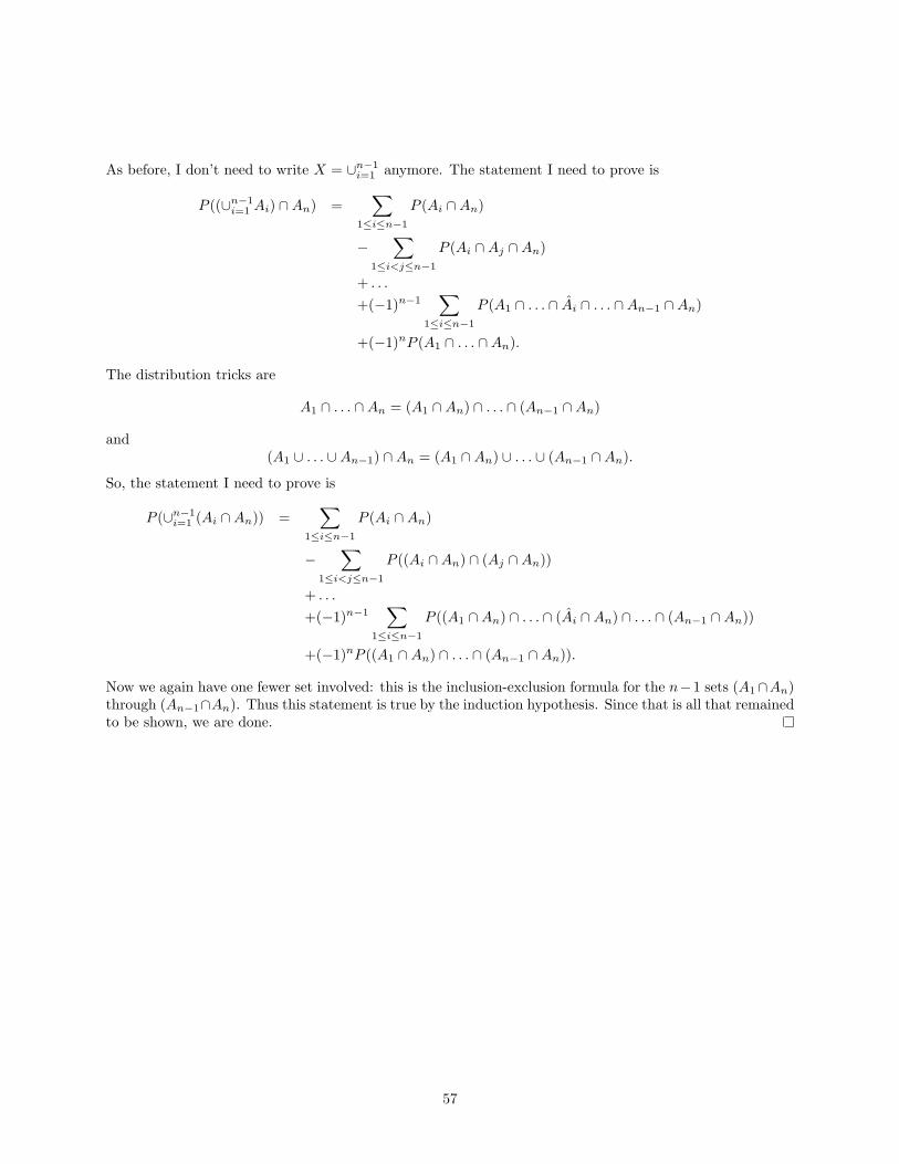
As before, I don’t need to write X = ∪n−1i=1 anymore. The statement I need to prove is
P ((∪n−1i=1 Ai) ∩An) =
∑1≤i≤n−1
P (Ai ∩An)
−∑
1≤i<j≤n−1
P (Ai ∩Aj ∩An)
+ . . .
+(−1)n−1∑
1≤i≤n−1
P (A1 ∩ . . . ∩ Ai ∩ . . . ∩An−1 ∩An)
+(−1)nP (A1 ∩ . . . ∩An).
The distribution tricks are
A1 ∩ . . . ∩An = (A1 ∩An) ∩ . . . ∩ (An−1 ∩An)
and(A1 ∪ . . . ∪An−1) ∩An = (A1 ∩An) ∪ . . . ∪ (An−1 ∩An).
So, the statement I need to prove is
P (∪n−1i=1 (Ai ∩An)) =
∑1≤i≤n−1
P (Ai ∩An)
−∑
1≤i<j≤n−1
P ((Ai ∩An) ∩ (Aj ∩An))
+ . . .
+(−1)n−1∑
1≤i≤n−1
P ((A1 ∩An) ∩ . . . ∩ (Ai ∩An) ∩ . . . ∩ (An−1 ∩An))
+(−1)nP ((A1 ∩An) ∩ . . . ∩ (An−1 ∩An)).
Now we again have one fewer set involved: this is the inclusion-exclusion formula for the n−1 sets (A1∩An)through (An−1∩An). Thus this statement is true by the induction hypothesis. Since that is all that remainedto be shown, we are done.
57
References
[Bha] Bhattacharya, R. Theoretical Statistics. Course notes, University of Arizona Math 567A, spring 2008.
[CB] Casella, G. and Berger, R.L. Statistical Inference (2nd ed.). Duxbury Press, 2001.
[Fol] Folland, G.B. Real Analysis: Modern Techniques and Their Applications (2nd ed.). Wiley-Interscience,1999.
[FG] Fristedt, B. and Gray, L. A Modern Approach to Probability Theory. Birkhauser, 1997.
[GS] Grimmett, G. and Stirzaker, D. Probability and Random Processes, 3rd ed. Oxford, 2001.
[Kennedy] Kennedy, T. Math 564. Course at University of Arizona, spring 2007.
[KK] Kaplan, M. and Kaplan, E. Chances Are . . . : Adventures in Probability. Penguin, 2007.
[MM] Moore, D.S. and McCabe, G.P. Introduction to the Practice of Statistics. Freeman and Co., 2005.
[Roy] Royden, H.L. Real Analysis (2nd ed.). MacMillan, 1968.
[Rud] Rudin, W. Principles of Mathematical Analysis (3rd ed.). McGraw-Hill, 1976.
58

59
Index
Aaction space . . . . . . . . . . . . . . . . . . . . . . . . . . . . . . . . . . . . .34almost surely . . . . . . . . . . . . . . . . . . . . . . . . . . . . . . . . . . . 30
BBayes risk . . . . . . . . . . . . . . . . . . . . . . . . . . . . . . . . . . . . . . .36Bayes rule . . . . . . . . . . . . . . . . . . . . . . . . . . . . . . . . . . . . . . 37Bayes’ theorem . . . . . . . . . . . . . . . . . . . . . . . . . . . . . . . . . .43Bernoulli distribution . . . . . . . . . . . . . . . . . . . . . . . . . . . . 9beta distribution . . . . . . . . . . . . . . . . . . . . . . . . . . . . . . . . 19bimodal . . . . . . . . . . . . . . . . . . . . . . . . . . . . . . . . . . . . . . . . . 17binomial distribution . . . . . . . . . . . . . . . . . . . . . . . . . . . . . 9bivariate normal distribution . . . . . . . . . . . . . . . . . . . . 27Borel σ-field . . . . . . . . . . . . . . . . . . . . . . . . . . . . . . . . . . . . 48
CCauchy distribution . . . . . . . . . . . . . . . . . . . . . . . . . . . . . 18Cauchy-Schwarz inequality . . . . . . . . . . . . . . . . . . . . . . 28CDF . . . . . . . . . . . . . . . . . . . . . . . . . . . . . . . . . . . . . . . . . . . . 17central limit theorem . . . . . . . . . . . . . . . . . . . . . . . . . . . . 31change of variables . . . . . . . . . . . . . . . . . . . . . . . . . . . . . . 25characteristic function . . . . . . . . . . . . . . . . . . . 15, 25, 50Chebyshev’s inequality . . . . . . . . . . . . . . . . . . . . . . . . . . 29coarsest . . . . . . . . . . . . . . . . . . . . . . . . . . . . . . . . . . . . . . . . . . 7conditional density . . . . . . . . . . . . . . . . . . . . . . .26, 37, 52conditional expectation . . . . . . . . . . . . . . 12, 26, 37, 51conditional PMF . . . . . . . . . . . . . . . . . . . . . . . . . . . . 12, 52conditional probability . . . . . . . . . . . . . . . . 8, 34, 43, 51confidence intervals . . . . . . . . . . . . . . . . . . . . . . . . . . . . . 32continuous random variable . . . . . . . . . . . . . . . . . . . . . 17convergence in distribution . . . . . . . . . . . . . . . . . . . . . . 31convergence in mean square . . . . . . . . . . . . . . . . . . . . . 29convergence in probability . . . . . . . . . . . . . . . . . . . . . . .29convolution . . . . . . . . . . . . . . . . . . . . . . . . . . . . . . . . . . . . . 16correlation coefficient . . . . . . . . . . . . . . . . . . . . . . . . . . . 27countable additivity . . . . . . . . . . . . . . . . . . . . . . . . . . 7, 49covariance . . . . . . . . . . . . . . . . . . . . . . . . . . . . . . . . . . . 27, 28cumulative distribution function . . . . . . . . . . . . . . . . .17
Ddecision rule . . . . . . . . . . . . . . . . . . . . . . . . . . . . . . . . . . . . 35density . . . . . . . . . . . . . . . . . . . . . . . . . . . . . . . . . . . . . . . . . .49discrete random variable . . . . . . . . . . . . . . . . . . . . . . . . . 9disjoint . . . . . . . . . . . . . . . . . . . . . . . . . . . . . . . . . . . . . . . . . . .7distribution . . . . . . . . . . . . . . . . . . . . . . . . . . . . . . . . . . . . . 49distribution function . . . . . . . . . . . . . . . . . . . . . . . . . . . . 49
Eevent . . . . . . . . . . . . . . . . . . . . . . . . . . . . . . . . . . . . . . . . . 7, 48
event space . . . . . . . . . . . . . . . . . . . . . . . . . . . . . . . . . . . . . . .7expectation . . . . . . . . . . . . . . . . . . . . . . . . . . . . . . . . . .11, 21expected value . . . . . . . . . . . . . . . . . . . . . . . . . . . . . . 11, 21experiment . . . . . . . . . . . . . . . . . . . . . . . . . . . . . . . . . . . . . . . 7exponential distribution . . . . . . . . . . . . . . . . . . . . . . . . . 18
Ffactorial . . . . . . . . . . . . . . . . . . . . . . . . . . . . . . . . . . . . . . . . .20factors . . . . . . . . . . . . . . . . . . . . . . . . . . . . . . . . . . . . . . . . . . 13finest . . . . . . . . . . . . . . . . . . . . . . . . . . . . . . . . . . . . . . . . . . . . .7Fourier transform . . . . . . . . . . . . . . . . . . . . . . . . . . . . . . . 50
Ggamma distribution . . . . . . . . . . . . . . . . . . . . . . . . . 19, 20gamma function . . . . . . . . . . . . . . . . . . . . . . . . . . . . . . . . .20geometric distribution . . . . . . . . . . . . . . . . . . . . . . . . . . . 10given . . . . . . . . . . . . . . . . . . . . . . . . . . . . . . . . . . . . . . . . . . . . . 8
Iidentically distributed . . . . . . . . . . . . . . . . . . . . . . . . . . . . 9IID . . . . . . . . . . . . . . . . . . . . . . . . . . . . . . . . . . . . . . . . . . . . . 14in distribution . . . . . . . . . . . . . . . . . . . . . . . . . . . . . . . . . . 31in mean square . . . . . . . . . . . . . . . . . . . . . . . . . . . . . . . . . .29in probability . . . . . . . . . . . . . . . . . . . . . . . . . . . . . . . . . . . 29Inclusion-exclusion formula . . . . . . . . . . . . . . . . . . . . . . 54independence . . . . . . . . . . . . . . . . . . . . . . . . . . . . . . . . . . . 51independent . . . . . . . . . . . . . . . . . . . . . . . . . . . 8, 13, 23, 51integrate away . . . . . . . . . . . . . . . . . . . . . . . . . . . . . . . . . . 22
JJacobian matrix . . . . . . . . . . . . . . . . . . . . . . . . . . . . . . . . .25joint CDF . . . . . . . . . . . . . . . . . . . . . . . . . . . . . . . . . . . . . . .22joint density . . . . . . . . . . . . . . . . . . . . . . . . . . . . . . . . . 13, 37joint PDF . . . . . . . . . . . . . . . . . . . . . . . . . . . . . . . . . . . . . . .22joint PMF . . . . . . . . . . . . . . . . . . . . . . . . . . . . . . . . . . . . . . 13jointly continuous . . . . . . . . . . . . . . . . . . . . . . . . . . . . . . . 22
LLaplace transform . . . . . . . . . . . . . . . . . . . . . . . . . . . . . . . 50law of large numbers, strong . . . . . . . . . . . . . . . . . . . . 30law of large numbers, weak . . . . . . . . . . . . . . . . . . . . . . 29Law of the Unconscious Statistician . . 11, 13, 21, 23law of total expectation . . . . . . . . . . . . . . . . . . . . . . . . . 12law of total probability . . . . . . . . . . . . . . . . . . . . . . . . . . . 8least-squared error . . . . . . . . . . . . . . . . . . . . . . . . . . . . . . 35loss function . . . . . . . . . . . . . . . . . . . . . . . . . . . . . . . . . . . . 35
Mmarginal . . . . . . . . . . . . . . . . . . . . . . . . . . . . . . . . . . . . 13, 22
60
marginal density . . . . . . . . . . . . . . . . . . . . . . . . . . . . . . . . 37mean . . . . . . . . . . . . . . . . . . . . . . . . . . . . . . 9, 11, 17, 18, 21measurable function . . . . . . . . . . . . . . . . . . . . . . . . . . . . . 49measurable sets . . . . . . . . . . . . . . . . . . . . . . . . . . . . . . . . . 48measurable space . . . . . . . . . . . . . . . . . . . . . . . . . . . . . . . .48measurable subset . . . . . . . . . . . . . . . . . . . . . . . . . . . . . . . . 7measure . . . . . . . . . . . . . . . . . . . . . . . . . . . . . . . . . . . . . . . . .49measure space . . . . . . . . . . . . . . . . . . . . . . . . . . . . . . . . . . .49median . . . . . . . . . . . . . . . . . . . . . . . . . . . . . . . . . . . . . . . . . .17method . . . . . . . . . . . . . . . . . . . . . . . . . . . . . . . . . . . . . .20, 24MGF . . . . . . . . . . . . . . . . . . . . . . . . . . . . . . . . . . . . . . . . . . . 15mode . . . . . . . . . . . . . . . . . . . . . . . . . . . . . . . . . . . . . . . . . . . 17moment-generating function . . . . . . . . . . . . . 15, 25, 50
Nnegative binomial distribution . . . . . . . . . . . . . . . . . . . 10normal distribution . . . . . . . . . . . . . . . . . . . . . . . . . . 19, 20normalization . . . . . . . . . . . . . . . . . . . . . . . . . . . . . . . . . . . 31normalize . . . . . . . . . . . . . . . . . . . . . . . . . . . . . . . . . . . . . . . 28
Oobservation space . . . . . . . . . . . . . . . . . . . . . . . . . . . . . . . 34observations . . . . . . . . . . . . . . . . . . . . . . . . . . . . . . . . . . . . 34outcome . . . . . . . . . . . . . . . . . . . . . . . . . . . . . . . . . . . . . . . . . .7
Ppairwise independent . . . . . . . . . . . . . . . . . . . . . . . . . . . . . 8parameter space . . . . . . . . . . . . . . . . . . . . . . . . . . . . . . . . .34parity . . . . . . . . . . . . . . . . . . . . . . . . . . . . . . . . . . . . . . . . . . . 52partition theorem . . . . . . . . . . . . . . . . . . . . . . . . . 8, 12, 51PDF . . . . . . . . . . . . . . . . . . . . . . . . . . . . . . . . . . . . . . . . 17, 49PMF . . . . . . . . . . . . . . . . . . . . . . . . . . . . . . . . . . . . . . . . . . . . . 9Poisson distribution . . . . . . . . . . . . . . . . . . . . . . . . . . . . . 10population . . . . . . . . . . . . . . . . . . . . . . . . . . . . . . . . . . . . . . 31population mean . . . . . . . . . . . . . . . . . . . . . . . . .14, 31, 35population space . . . . . . . . . . . . . . . . . . . . . . . . . . . . . . . . 34population variance . . . . . . . . . . . . . . . . . . . . . . . . . . . . . 14posterior distribution . . . . . . . . . . . . . . . . . . . . . . . . . . . .37posterior expected loss . . . . . . . . . . . . . . . . . . . . . . . . . . 38posterior mean . . . . . . . . . . . . . . . . . . . . . . . . . . . . . . . . . . 37preimage . . . . . . . . . . . . . . . . . . . . . . . . . . . . . . . . . . . . . . . . . 9prior distribution . . . . . . . . . . . . . . . . . . . . . . . . . . . . . . . .36probability density function . . . . . . . . . . . . . . . . . 17, 49probability mass function . . . . . . . . . . . . . . . . . . . . . . . . .9probability measure . . . . . . . . . . . . . . . . . . . . . . . . . . 7, 49probability measures . . . . . . . . . . . . . . . . . . . . . . . . . . . . 34probability space . . . . . . . . . . . . . . . . . . . . . . . . . .7, 34, 49
Rrandom variable . . . . . . . . . . . . . . . . . . . . . . . . . . . . . . 9, 49range . . . . . . . . . . . . . . . . . . . . . . . . . . . . . . . . . . . . . . . . . . . 25risk function . . . . . . . . . . . . . . . . . . . . . . . . . . . . . . . . . . . . 35
Ssample . . . . . . . . . . . . . . . . . . . . . . . . . . . . . . . . . . . . . . 29, 31sample mean . . . . . . . . . . . . . . . . . .14, 24, 29, 31, 35, 40sample space . . . . . . . . . . . . . . . . . . . . . . . . . . . . . .7, 34, 48σ-field . . . . . . . . . . . . . . . . . . . . . . . . . . . . . . . . . . . . . . . . 7, 48standard deviation . . . . . . . . . . . . . . . . . . . . . . . . . . . . . . 11standard normal distribution . . . . . . . . . . . . . . . . 19, 20standardization . . . . . . . . . . . . . . . . . . . . . . . . . . . . . .31, 40strong law of large numbers . . . . . . . . . . . . . . . . . . . . . 30
Ttotal expectation, law of . . . . . . . . . . . . . . . . . . . . . . . . 12total probability, law of . . . . . . . . . . . . . . . . . . . . . . . . . . 8
Uunbiased estimator . . . . . . . . . . . . . . . . . . . . . . . . . . . . . . 34uncorrelated . . . . . . . . . . . . . . . . . . . . . . . . . . . . . . . . . . . . 14uniform distribution . . . . . . . . . . . . . . . . . . . . . . . . . . . . .18
Vvariance . . . . . . . . . . . . . . . . . . . . . . . . . . . 9, 11, 18, 21, 28
Wweak law of large numbers . . . . . . . . . . . . . . . . . . . . . . 29with probability one . . . . . . . . . . . . . . . . . . . . . . . . . . . . .30
Zz-score . . . . . . . . . . . . . . . . . . . . . . . . . . . . . . . . . . . . . . 32, 40
61