near-real-time characterization of stockpiled soils
TRANSCRIPT

BNL-71393-2003
The BNL ASTD Field Lab – Near-Real-time Characterization of BNL Stockpiled Soils to Accelerate
Completion of the EM Chemical Holes Project
B.S. Bowerman, J.W. Adams, J. Heiser, P.D. Kalb, and A. Lockwood
April 2003
Brookhaven National Laboratory Upton, New York 11973-5000

BNL-71393-2003
The BNL ASTD Field Lab – Near-Real-time Characterization of BNL Stockpiled Soils to Accelerate
Completion of the EM Chemical Holes Project
B.S. Bowerman, J.W. Adams, J. Heiser, P.D. Kalb, and A. Lockwood
April 2003
Environmental Research and Technology Division Environmental Sciences Department
Brookhaven National Laboratory
P.O. Box 5000 Upton, NY 11973-5000
www.bnl.gov
Managed by Brookhaven Science Associates, LLC
for the United States Department of Energy under Contract No. DE-AC02-98CH10886
*This work was performed under the auspices of the U.S. Department of Energy.
DISCLAIMER
This report was prepared as an account of work sponsored by an agency of the United States Government. Neither the United States Government nor any agency thereof, nor any of their employees, nor any of their contractors, subcontractors or their employees, make any warranty, express or implied, or assumes any legal liability or responsibility for the accuracy, completeness, or any third party’s use or the results of such use of any information, apparatus, product, or process disclosed, or represents that its use would not infringe privately owned rights. Reference herein to any specific commercial product, process, or service by trade name, trademark, manufacturer, or otherwise, does not necessarily constitute or imply its endorsement, recommendation, or favoring by the United States Government or any agency thereof or its contractors or subcontractors. The views and opinions of author’s expresses herein do not necessarily state to reflect those of the United States Government or any agency thereof.

Executive Summary As of October 2001, approximately 7,000 yd3 of stockpiled soil remained at Brookhaven National Laboratory (BNL) after the remediation of the BNL Chemical/Animal/Glass Pits disposal area. The soils were originally contaminated with radioactive materials and heavy metals, depending on what materials had been interred in the pits, and how the pits were excavated. During the 1997 removal action, the more hazardous/radioactive materials were segregated, along with, chemical liquids and solids, animal carcasses, intact gas cylinders, and a large quantity of metal and glass debris. Nearly all of these materials have been disposed of. In order to ensure that all debris was removed and to characterize the large quantity of heterogeneous soil, BNL initiated an extended sorting, segregation, and characterization project directed at the remaining soil stockpiles. The project was co-funded by the Department of Energy Environmental Management Office (DOE EM) through the BNL Environmental Restoration program and through the DOE EM Office of Science and Technology Accelerated Site Technology Deployment (ASTD) program. The focus was to remove any non-conforming items, and to assure that mercury and radioactive contaminant levels were within acceptable limits for disposal as low-level radioactive waste. Soils with mercury concentrations above allowable levels would be separated for disposal as mixed waste. Sorting and segregation were conducted simultaneously. Large stockpiles (ranging from 150 to 1,200 yd3) were subdivided into manageable 20 yd3 units after powered vibratory screening. The ½-inch screen removed almost all non-conforming items (plus some gravel). Non-conforming items were separated for further characterization. Soil that passed through the screen was also visually inspected before being moved to a 20 yd3 “subpile.” Eight samples from each subpile were collected after establishing a grid of four quadrants: north, east, south and west, and two layers: top and bottom. Field personnel collected eight 100-gram samples, plus quality assurance (QA) duplicates for chemical analysis, and a 1-liter jar of material for gamma spectroscopy. After analyses were completed and reviewed, the stockpiles were reconstructed for later disposal as discrete entities within a disposal site profile. A field lab was set up in a trailer close to the stockpile site, equipped with instrumentation to test for mercury, RCRA metals, and gamma spectroscopy, and a tumbler for carrying out a modified Toxicity Characteristic Leaching Procedure (TCLP) protocol. Chemical analysis included X-ray fluorescence (XRF) to screen for high (>260 ppm) total mercury concentrations, and modified TCLP tests to verify that the soils were not RCRA hazardous. The modified TCLP tests were 1/10th scale, to minimize secondary (leachate) waste and maximize tumbler capacity and sampler throughput. TCLP leachate analysis was accomplished using a Milestone Direct Mercury Analyzer (DMA80). Gamma spectroscopy provided added assurance of previously measured Am-241, Cs-137, and Co-60 contamination levels. The ASTD field laboratory completed more than 2,500 analyses of total Hg (XRF) and TCLP/DMA analyses over an 18-week period. Reliable statistical verification was accomplished for more than 98% of the stockpile subpiles. For most subpiles, TCLP analyses were completed within two days. One of the most significant aspects of the project success was schedule
i

acceleration. The original schedule projected activities extending from early April until September 30. Due to efficiency and reliability of the vibratory screening operation and cooperative, dry summer weather, stockpile reconstruction was completed in the third week of August. Reduction of the planned sample collection rate, from three samples per five cubic yards to two, resulted in further schedule acceleration. The resulting sample frequency, however, was still 22 times greater than the baseline frequency (1 per 55 yd3).
ii

Table of Contents Executive Summary ......................................................................................................................... i 1. Introduction................................................................................................................................ 1 2. Project Planning......................................................................................................................... 2
2.1 Stockpile Sorting and Sampling........................................................................................... 3 2.2 ASTD Field Laboratory ....................................................................................................... 5 2.3 Field Laboratory Analytical Methods.................................................................................. 6
2.3.1 X-ray Fluorescence ....................................................................................................... 6 2.3.2 Anodic Stripping Voltammetry..................................................................................... 7 2.3.3 Direct Mercury Analyzer .............................................................................................. 7 2.3.4 Modified TCLP............................................................................................................. 7 2.3.5 In Situ Object Counting System.................................................................................... 8 2.3.6 Integrated Operations and Quality Assurance .............................................................. 8
3. Work Completed........................................................................................................................ 9 3.1 Sample Production Rates and Chemical Analysis Capacity................................................ 9 3.2 Field Laboratory Results.................................................................................................... 11
3.2.1 ISOCS Results ............................................................................................................ 12 3.2.2 Total Mercury and TCLP Mercury Results ................................................................ 12
4. Discussion and Conclusions .................................................................................................... 13 4.1 Comparison with Off-site Results...................................................................................... 14 4.2 Comparison with 2001 Sampling Campaign Results ........................................................ 18 4.3 Conclusions........................................................................................................................ 18
5. References................................................................................................................................ 19 Appendices.................................................................................................................................... 32
iii
1. Introduction Approximately 11,500 cubic yards (yd3) of contaminated soil were excavated from Brookhaven National Laboratory’s (BNL) former Animal/Chemical and Glass Holes (Chemical Holes) in 1997 as part of activities required under the Comprehensive Environmental Response, Compensation, and Liability Act (CERCLA, or Superfund). The Chemical Holes remedial action was initiated to remove laboratory glassware, chemicals, and related wastes from disposal pits used at BNL from 1958 through 1976. The soils were placed into separate stockpiles and characterized following an approved sampling plan (Procedure for Sampling Soil Stockpiles Chemical Holes Project, BNL, October 1997). As part of the removal action, the materials removed from the pits were segregated according to size and type. Larger items were collected manually, and the remaining materials were separated using a 2-inch screen. The remaining (less than 2-inch) material, consisting mostly of soil and gravel, but also including small bottles and vials potentially containing hazardous material, was collected and stored in 18 stockpiles at the removal project site. The stockpiles range in size from 100 yd3 to 1,800 yd3. In the ensuing years, some of the stockpile soils, which had been characterized as non-radioactive and non-hazardous, were disposed at Subtitle D facilities. During the removal action, the more hazardous/radioactive materials were segregated, along with a large quantity of metal and glass debris. Nearly all of these latter materials have been disposed of. The majority of the stockpiled soil had been identified as low-level radioactive waste (LLW). One stockpile (Stockpile 12, 700 yd3) was to be handled as mixed waste based on the presence of visible mercury reported by workers during the original removal action. From September 1999 to January 2000, 29 railcars that included materials from Stockpiles 10 and 13 were shipped to Envirocare of Utah for LLW disposal after obtaining the appropriate approvals. Envirocare’s routine sampling program (every 10th rail car) indicated that the Stockpile 10 soils exceeded RCRA criteria for allowable mercury levels of 0.2 mg/L in TCLP leachate. Subsequently, some of the Stockpile 10 soils were re-classified as mixed waste, treated (stabilized), and disposed of at Envirocare. This resulted in a non-conformance incident, and significant additional treatment/disposal costs (nearly $450,000). Additional costs were identified at BNL before all the waste materials were shipped in this period. During loading of some of these wastes for disposal, “non-conforming items” were identified (e.g., vials, bottles, etc. less than 2 inches and potentially containing hazardous materials such as mercury) still entrained in the waste soil, requiring that about 380 yd3 of soil from Stockpile 13 be sorted a second time. Evaluations of the root causes of the Envirocare non-conformance incident focused on the need for improved segregation of non-conforming items, as well as improved sampling and analysis protocols applied to the stockpiles for characterization. Thus, manual hand raking of non-conforming items from the remaining portion of Stockpile 13 was initiated. This was the baseline sorting technique, but it proved to be an extremely slow, labor-intensive, and expensive process. Following the occurrence investigation (ORPS No. CH-BH-BNL-BNL-2000-0002), the Bulk Waste Determination Guidance Document (also referred to here as the Toolbox [1]) was prepared, based on sampling protocols identified in EPA SW-846. This procedure represents the baseline characterization currently in place for the stockpiles prior to disposal. While intended to
1

provide a standard method for characterizing remaining stockpiles, it requires relatively few samples be taken for large volumes of contaminated soil. For example, application of this methodology to Stockpile 6B, which contained a total of 440 yd3 of soil, resulted in identification of only 8 soil samples for analysis. In the application of the procedure, an interactive spreadsheet (referred to as the Toolbox) is used to input characterization data. The Toolbox then gives an evaluation as to whether additional samples are needed for characterization to a 95% confidence level. In order to continue disposal efforts and improve performance, BNL tested a powered ½-inch screen sorting method on Stockpile 6B, and conducted characterization sampling following the Toolbox method. Stockpile 6B was shipped and disposed of without incident in July 2001. As part of this effort, ten samples were collected from each of the other stockpiles, and analyzed for TCLP and total inorganic constituents. As of October 2001, approximately 7,000 yd3 of soil in 10 stockpiles still remained, requiring final disposition. To prevent more non-conformance incidents (and potential regulatory problems) during subsequent soil disposal activities, BNL initiated an expanded sorting, segregation, and characterization project directed at the ten remaining soil stockpiles. The project was co-funded by the BNL Environmental Restoration program and the DOE EM Office of Science and Technology Accelerated Site Technology Deployment (ASTD) program. The focus was to remove non-conforming items and assure that mercury and radioactive contaminant levels were within acceptable levels for disposal as low-level radioactive waste. Extensive sampling was planned to provide a sound statistical basis for confidence in the measured contaminant levels. Soils with mercury concentrations above allowable levels would be separated for disposal as mixed waste. The project involved the use of a power screen for sorting and segregation, and setting up and operating a field laboratory near the stockpile area that would provide rapid sample analyses for total mercury, other RCRA metals, and TCLP mercury. Samples were to be collected and carried to the field lab for analysis with a planned one-day turnaround. Cost-effective, timely analysis of soil contamination allowed many more samples be taken and analyzed, significantly improving confidence in the data. The next two sections describe planning and preparation for the project, and the work completed. The final section compares the ASTD Field Lab to off-site and duplicate results, and discusses lessons learned. 2. Project Planning The main project goals were:
1. The complete removal of all non-conforming items in a safe manner from the soil stockpiles, and
2. The analysis of each stockpile for total mercury and TCLP mercury, to demonstrate in a statistically reliable manner that the soil is non-hazardous on average.
2

2.1 Stockpile Sorting and Sampling The first goal involved the use of the power screening method applied to Stockpile 6B, as mentioned earlier. During the screening, soils were to be separated into 20 yd3 subpiles for sampling and subsequent analysis. A field laboratory, set up in a trailer near the stockpile area, was to be the means of achieving the second goal. The field lab would have the capability to test soils directly for total mercury, and would conduct modified TLCP extractions and test the extract for mercury. Finally, an ISOCS unit would collect gamma spectra for radiological characterization. BNL’s EM Directorate completed the plans for the sorting and segregation activities. A health and safety plan [2], a sampling and analysis plan [3], and a technical work document [4] were prepared, following BNL EM standard procedures. The Environmental Research and Technology Division (ERTD) was responsible for the field laboratory and, prepared similar plans for its operation [5, 6]. Based on the earlier work with Stockpile 6B, stockpile sorting rates were estimated at a maximum of 100 yd3 per day, or five 20 yd3 subpiles per day. Sampling and analysis plans were designed around this sorting volume estimate and the assumption that 3 samples were to be collected for every 5 yd3. Three samples per 5 yd3 were considered more than adequate for statistical certainty, particularly in comparison to the 1 sample per 55 yd3 determined to be acceptable for Stockpile 6B with the Toolbox. Crumbling, et al [7] reported that uncertainty in environmental characterization is often a trade-off involving the number of samples and sampling methods, field screening analysis methods, and certified analytical laboratory methods. While precision in analytical methods has been steadily increasing with improved technology, accuracy in characterization is much more dependent on how well the sample reflects the actual condition of the waste. Uncertainty in the data therefore is much more closely tied to the extent of sampling. In many environmental remediation characterization efforts, sampling uncertainty offsets analytical laboratory reliability. Explicitly: “If representativeness cannot be established, the quality of the chemical analysis is irrelevant.” [7] Data quality in support of remediation decisions can be improved considerably with increased sampling and field screening methods to supplement certified laboratory results. Soil stockpiles were located in two areas, shown as green rectangles on the map in Figure 1. For eight of the stockpiles, the power-screen was set up at the former Glass Holes Area between Stockpiles 12 and 8. (The power-screen is shown in Figure 2.) As sorting progressed and soil from each stockpile was placed as 20 yd3 subpiles with a front-loader, samples were collected from the subpiles. The subpiles were placed in the area to the southeast of the power-screen, south of Stockpile 15, wet of and adjacent to the woods. This served as the staging area for stockpile reconstruction in the Animal/Chemical Pits Area (also shown in Figure 1 as red-outlined rectangles). Subpiles were placed on 3-mil polyethylene sheets, and, after sampling, covered with polyethylene as well, until reconstruction was approved. Once the eight stockpiles in the Glass Holes area were sorted and reconstructed, the power-screen was moved to the Animal Chemical pits area for sorting the last two stockpiles, 6C and 6R.
3
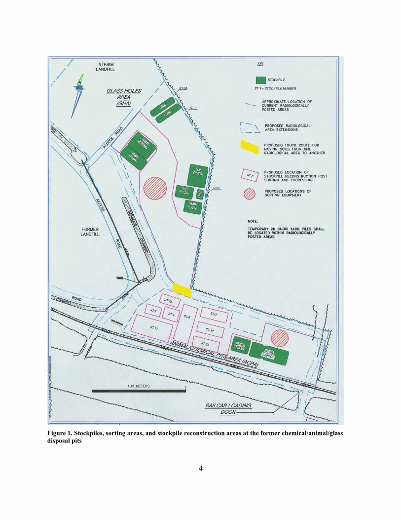
Figure 1. Stockpiles, sorting areas, and stockpile reconstruction areas at the former chemical/animal/glass disposal pits
4

Figure 2. The half-inch vibratory screen unit (Powerscreen Chieftain 600)
2.2 ASTD Field Laboratory Samples from the subpiles were transported to the ASTD Field Laboratory for analysis each day they were collected. As noted earlier, 60 samples per day were expected, based on Stockpile 6B sorting experience. Sample analysis procedures were based on this throughput estimate, and on testing each sample for total mercury and most (but not all) samples using a modified EPA Toxicity Characteristic Leaching Procedure (TCLP). Originally, the testing scheme was to follow that shown in Figure 3. X-ray Fluorescence (XRF) was to be used as a screening tool to measure total mercury in the soil sample, since this mercury detection limit was identified by the manufacturer as achievable in solids with an analysis time of between 5 and 10 minutes. If mercury concentration for a sample was above 10 ppm, total mercury measurements were to be verified using the PDV 5000, and the sample was to be tested using the modified TCLP. If the XRF indicated that the sample was below 10 ppm mercury, the total mercury was to be verified with the Milestone Direct Mercury Analyzer (DMA) or the PDV 5000. From the latter test, if total mercury was less than 4 ppm, no further testing was deemed necessary, since a concentration of < 4 ppm total mercury could not result in TCLP concentrations in excess of the TCLP allowable limit of 0.2 ppm, assuming all of the mercury was leached. If more than 4ppm was detected, TCLP was still required. TCLP failure means that the results for a particular subpile would have to be reviewed and averaged, to determine if the subpile or a portion of it had to be segregated for ultimate hazardous or mixed waste disposal. The Toolbox [Ref. 1] provides algorithms for determining the acceptability of the averages and confidence levels for subpiles and whole stockpiles.
5

In addition to the chemical analyses, the ASTD Field Lab also collected radiological content information using the In Situ Object Counting System (ISOCS) to determine the presence of gamma-emitting radionuclides.
Figure 3. Planned process diagram for innovative waste segregation and near-real-time characterization of stockpiled soils
2.3 Field Laboratory Analytical Methods 2.3.1 X-ray Fluorescence X-ray Fluorescence (XRF) is a mature technology that has been used for decades for elemental analysis in research laboratories and industrial process monitoring. Detection limits to between 10 and 100 ppm are easily achieved for most elements. With higher strength X-ray sources and secondary targets, sensitivities as low as 1.0 ppm or less are also possible. The Model EX-6600A field-deployable XRF unit was purchased for this project from Jordan Valley; the reported detection limit for mercury was 1.5 ppm.
An important advantage of the XRF method is that sample preparation is minimal, and, for mercury, the RCRA metal of concern in this project, detection can be achieved in air or a helium-flushed system, rather than vacuum. XRF is a non-destructive method that can be applied to solid, powdered, or liquid samples. Generally, no secondary wastes are generated as a result of sample preparation. Sample analysis time, including preparation, was expected to be approximately 10 minutes. A 10-position automatic sample-changer was included in the purchased unit.
6

2.3.2 Anodic Stripping Voltammetry The PDV 5000 was chosen for the project because it promised to be an inexpensive, simple, rapid technique for analyzing mercury and other toxic metals. It is a commercially available version of a method that in the past had been generally relegated to research laboratories. The method involves anodic stripping voltammetry (ASV), in which metals in solution are first electroplated onto an electrode. After this, current is reversed to strip the metals from the electrode back into solution. Each metal becomes stripped at a characteristic voltage, and the current density at that voltage is proportional to the total quantity of metal.
Because ASV involves the analysis of liquids, applications have usually focused on process liquid monitoring. Environmental applications have included river water testing for mercury and other metals. For soil testing, metals can be detected and quantified electrochemically after acid digestion with an acidic electrolyte. With the metal constituents in solution, electroplating followed by anodic stripping becomes possible. The detection limit for mercury in field applications was stated as 0.01 ppm in the liquid, which, according to the published procedure, corresponds to 0.02 ppm in the soil matrix. 2.3.3 Direct Mercury Analyzer The Milestone DMA-80 measures low concentrations of mercury in environmental samples, in accordance with EPA Method 7473, “Mercury In Solids And Solutions By Thermal Decomposition, Amalgamation, and Atomic Absorption Spectrophotometry.” Its reproducibility, low detection limits, rapid throughput, and the fact that it does not generate any secondary waste, makes it ideally suited for environmental applications. The method involves weighing the sample and placing it directly in a small “boat,” for drying and thermal treatment in a stream of heated oxygen gas. The gas stream is passed through a gold amalgamation trap that captures all mercury in the vapor phase. The gold amalgam is subsequently heated and mercury vapor detected with an atomic absorption spectrophotometer tuned to the absorption wavelength for mercury, 254 nm. The Milestone DMA detection limit is 0.11 nanograms mercury. For the listed maximum sample size of 0.5 grams, therefore, the theoretical detection limit in terms of concentration is 0.00022 ppm (0.22 ppb). 2.3.4 Modified TCLP The modified Toxicity Characteristic Leaching Procedure (TCLP) used was essentially a 1/10th scale version of the test recommended by the U.S. Environmental Protection Agency (EPA) [Ref. 8]. Extraction fluid #1 was used for all tests, as determined by the related EPA procedure [Ref. 9]. Soil samples of 10 gram size (rather than 100 g) were weighed out in 250 mL plastic bottles, and 200 mL (rather than 2L) of fluid #1 was added to the soil. Five leach samples in small bottles were placed inside a plastic 1-gallon jar to serve as secondary containment, which was then placed into a compartment of the tumbler apparatus. A TCLP tumbler purchased from Miller Analytical, with 12 compartments, allowed for 60 samples to be tested simultaneously. The samples were tumbled for 18 hours, per the TCLP procedure. The modified small-scale
7

procedure meant that more samples could be tumbled concurrently, and less waste was produced. Results were reported as parts per million (ppm) or parts per billion (ppb) TCLP mercury, representing mercury concentration in the leach solution, not the solid. 2.3.5 In Situ Object Counting System The Canberra In Situ Object Counting System (ISOCS) consists of a portable germanium detector controlled by proprietary software for detector calibration and evaluation of specific activity. Standard sample configurations with shielding may be used, or large areas or equipment may be surveyed with the detector, provided models are available for geometric data interpretation. ISOCS has been used at BNL in two earlier ASTD projects. For the Chemical Holes Field Lab, a standard sample configuration was used for verifying gamma-emitting radionuclide contamination in the stockpiles. One sample per 20 yd3 subpile was counted. 2.3.6 Integrated Operations and Quality Assurance Since the stockpiles had been classified as low-level waste, the field lab was set up as a radioactive materials area for sample storage. Sample handling, namely opening bottles, weighing out soils, and preparing TCLP bottles for tumbling, was carried out in the west half of the trailer. Because of the potential for loose soil releases in this half of the lab, it was designated as a radioactive dispersibles area when transfer operations were being conducted. The XRF, PDV5000, and DMA-80 were also located in this section. The east end of the lab trailer was used for receiving samples, ISOCS counting, and running the TCLP tumbling apparatus. A schematic layout of the Lab is shown in Figure 4. Sample receipt involved signing Chain of Custody (COC) forms after verifying that all bottles were labeled clearly and that the COC information was correct. ISOCS samples were to be stored and counted in the east end of the trailer. The remainder of the samples was to be transferred for processing and analysis by the chemical techniques described above. After a targeted one-day turnaround, analytical results were compiled and transferred to the Project Manager for review. Unused soils and liquid extracts were returned to the stockpiles for final disposal. When all data for a stockpile had been reviewed, the Project Manager approved stockpile reconstruction. The criteria for reconstruction were that the soils contained less than 260 ppm total mercury and less than 0.2 ppm TCLP mercury. Quality assurance focused on maintaining proper chain of custody protocols and taking a subset of field duplicates: one for analysis in the ASTD Field Lab, and one for analysis at an independent off-site laboratory. In addition, the analytical instruments were to be calibrated according to manufacturer’s recommended guidelines.
8

Figure 4. ASTD Field Lab - Schematic layout
3. Work Completed 3.1 Sample Production Rates and Chemical Analysis Capacity Sorting began the first week of May, 2002, on Stockpile 8. After about 2 weeks, the soil sorting team had developed a standard routine for their activities, and they were processing more than 100 yd3 per day. In fact, on their best days they processed as much as 230 yd3, or more than twice the originally projected capacity. This resulted in a significantly higher production of analytical samples than was anticipated (60 samples per day). In addition to receiving more samples than planned for, ASTD Field Lab operations required modification due to poor performance of the PDV 5000 (primarily unsatisfactory reproducibility) which eventually resulted in eliminating this method from the suite of analyses (see discussion below). Consequently a revised analytical strategy was implemented to improve productivity and provide the critical data needed for decision-making on the status of individual soil stockpiles. These three essential criteria were:
9

· confirmation that total mercury levels were < 260 ppm · evaluation of TCLP mercury levels to ensure they did not exceed 0.2 ppm · radiological analysis Specifically, the XRF was used to screen for >260 ppm total mercury and the DMA-80 was assigned to measure mercury exclusively in the TCLP leachates. The DMA-80 was assigned for TCLP results because it could be used for liquid as well as solid samples and gave highly reproducible results, as evidenced by blank and calibration standards tested after every five samples. With the DMA-80, preparation of the TCLP leach liquids for analysis was minimal, namely filtering the solution (0.45 µ) and pipetting 0.4 mL. Because of its reproducibility, the DMA-80 was deemed most important for application to the regulatory compliance test. The XRF was assigned to total mercury analysis, but the procedure was modified to shorten preparation and analysis time. The Jordan Valley EX-6600 had been chosen because the company demonstrated detection limits of less than 10 ppm total mercury on samples provided by BNL. However, this was accomplished after milling/grinding the samples for ten minutes, and pressing the fine powder into pellets with a hydraulic press. With these steps, sample preparation time was about twenty minutes per sample, far too long for the throughput needed for the field lab application. In addition, the counting time on the x-ray unit was about fifteen minutes per sample. A shorter sample preparation time was developed which required sieving the soil to less than 2 mm and compacting it in a disposable plastic cup with a transparent Mylar film bottom. This and a 5-minute analysis time meant that the detection limit for the samples was approximately 20 ppm total mercury. The higher detection limit meant that the XRF unit was best used as a screening tool for higher levels of mercury, i.e. more than 260 ppm. Soils with this high a concentration require treatment before disposal under EPA land disposal restrictions. After Stockpile 15 was completed, it was determined that a shorter analysis time of 3 minutes, with a detection limit of 50 ppm was necessary to analyze 60 samples per day. The PDV 5000 was dropped from use because reproducibility of calibration standards with it was often less than 20%. Discussions with the instrument manufacturer failed to resolve the issue completely, primarily because there was insufficient man-power to work on the recommended method modifications. Anodic stripping voltammetry depends on obtaining reproducibly dissolved mercury analyte in an interference-free electrolyte solution. It was not clear from the limited tests conducted whether:
1. Interfering elements were present in the soils and were being dissolved along with mercury,
2. The acid solution used was not dissolving mercury reproducibly from the soils, or 3. The active carbon electrode on the instrument was becoming fouled.
The revised laboratory procedure process flow diagram is shown in Figure 5. Several weeks were required to make all adjustments, and several important decisions about the data requirements were needed to make data production match sample production. The most important decision was to reduce the sample collection rate from three for every five cubic yards
10

to two. The resulting sample frequency (1 per 2.5 yd3) was still 22 times greater than the baseline frequency (1 per 55 yd3).
Non-conforming Items
Segregate for Mixed Waste
Disposal
VibratoryScreen
20 yd3
Subpiles
<260ppm
No
Yes
X-ray Fluorescence Spectrometer (XRF)
Direct Mercury Analyzer
Reconstruct Stockpile for
LLW Disposal<0.2ppm
Yes No
7000 yd3
Stockpiles
TCLPSamples
Segregate for Mixed Waste
Treatment
Figure 5. Final sorting and analysis scheme for ASTD Field Lab
3.2 Field Laboratory Results Table 1 compares original estimated stockpile volumes to those determined during sorting operations. Stockpile sorting included moving sorted soils from the power-screen to the subpile staging area with a 1-yd3 front-loader. Thus, the soil stockpile volumes were measured more accurately than when they were accumulated initially, because the subpiles were built to a specified number of front-loader loads. Overall, the total screened soil volume, 5,660 yd3, was smaller than the original estimate of 6,790 yd3. Final disposal volume may also be slightly smaller, depending on how much compaction occurs during loading and transport in railcars. Some of the volume reduction may be associated with the separation of old plastic cover material, which had been covered with new layers, as weather-induced tears required the replacement of the first covers. All cover materials were segregated for disposal as debris.
11

Soil sorting activities produced 283 subpiles, which were then re-assembled into ten new stockpiles, corresponding to the original ten. Radioactive measurements with the ISOCS unit and chemical test results are discussed separately. 3.2.1 ISOCS Results The number of samples collected for ISOCS analysis totaled 283, or 1 for each subpile. Results are listed in full in Appendix 1, and summarized by stockpile in Table 2. The results include average values, maximum values, and the total number of non-detected measurements (NDs) for each stockpile. These quantities show that the stockpiles are slightly contaminated, overall. Previous characterization data indicated that radioactive contamination was low and restricted to a few radionuclides, primarily cesium-137 (Cs-137) and americium-241 (Am-241). These general results are verified with the additional ISOCS data. Other isotopes detected include cobalt-60 (Co-60), radium-226 (Ra-226), thorium-232 (Th-232), and uranium-235 (U-235). Of all these isotopes, Ra-226 and Th-232 are potentially naturally occurring at low levels because of Long Island’s geology [10]. All are associated with some aspect of nuclear power or research, e.g., fuel (U-235, Th-232), fuel by-products and waste (Co-60, Cs-137) or isotope application studies (Co-60, Cs-137, Am-241, Ra-226, Th-232). Am-241 had the highest levels of contamination, with 4 readings greater than 10 pCi/g. in 4 separate stockpiles. It is worth noting that in 3 of these stockpiles (St-6A, St-11, and St-12) more that half of the subpiles had Am-241 non-detects, and in the fourth stockpile, 11 out of 34 subpiles were non-detected for Am-241. It is also significant that the average Am-241 values for the stockpiles were all less than 5 pCi/g, and that Am-241 was the only radionuclide that exhibited a concentration in excess of 1.0 pCi/g. Cs-137 has been identified as a radionuclide of concern at BNL, and cleanup levels for it are set at 23 pCi/g. The maximum concentration of Cs-137 found was 2.3 pCi/g in a subpile from Stockpile 11. The highest average concentration for a stockpile was 0.8 pCi/g, for St-7. 3.2.2 Total Mercury and TCLP Mercury Results The total number of chemical analyses performed in this project was in excess of 2,264 (8 times 283). During sorting and sampling of the first stockpile, St-8, it was immediately obvious that stockpile soils were being screened and sampled at a rate that far exceeded the field lab’s projected daily capacity. To keep up with sample production, the center level sample from the three-level sampling grid was ignored. Thus only four samples from the top and four from the bottom level quadrants were actually analyzed. Further, because it was being used as a higher-concentration screening tool, XRF analysis was performed on 132 fewer samples (for Stockpiles 3, 4, and 8). (These can be identified in Appendix 2, which lists all total mercury and TCLP mercury results side-by-side.) After Stockpile 8 was completed, the sampling plan was modified so that 8 rather than 12 samples were collected for every 20 yd3 (or 2 for every 5 cubic yards). Additionally, a sample for offsite analysis and a field duplicate (FD) were collected for every 20th sample. For Stockpile 8, 28 of 132 “center level” samples collected were analyzed for
12

TCLP (subpiles 1 to 3 and 20 to 23, inclusive). Thus, TCLP analyses in the ASTD Field Lab totaled 2,406 (2,264 + 28 + 114 FDs). There were a total of 2,246 XRF analyses. Table 3 lists average total and TCLP mercury concentrations for each stockpile. Stockpile 7 had the highest total mercury concentration of 65.1 (± 2.8) mg/kg, well below the EPA action level of 260 mg/kg for which treatment is required. Stockpile 6C showed the highest statistical deviation of about 20% (or 57.5 ± 12.0 mg/kg), and Stockpile 3 was uniformly at the detection limit of 18.8 mg/kg total mercury. (Recall that later measurements with a shorter run time meant that the minimum detection level for stockpiles tested after St-15 was 50.5 mg/kg). The highest subpile average for total mercury was 86.6 mg/kg in St-6C. Stockpile 6C also had the highest single sample total mercury value at 174.0 mg/kg. In all, there were 16 single samples above 100 ppm, and these were distributed over 5 stockpiles. Stockpiles 8, 3, 4, 6A, and 7 had no samples with total mercury concentration greater than 100 ppm. More importantly, in terms of classifying the soils as hazardous or mixed wastes, stockpile averages for TCLP mercury are all well below 200 µg/L, the hazardous waste definition for EPA’s Toxicity Characteristic. As can be seen in Table 3, the stockpile TCLP mercury averages are well below the BNL administrative action level of 160 µg/L. Stockpile 12 had the highest levels of TCLP mercury, at 73.0 (± 29.6) µg/L. This is consistent with Stockpile 12 having the highest subpile average TCLP of 153.7 µg/L, and 5 subpiles with average TCLP mercury above 100 µg/L (see Table 4). As can be seen in Table 4, only two other subpiles, one in Stockpile 11 and one in Stockpile 6R, had an average TCLP mercury level above 100 µg/L. There were 14 individual samples with TCLP mercury above the administrative action level of 160 µg/L, as listed below, from Stockpiles 11, 12, and 6R. When TCLP leachate samples above the 160 µg/L level were found, the original leachates were re-analyzed in the DMA to verify the levels. Those shown below were the higher of the two test results. Stockpiles 3, 4, 6A, 6C, 7, 8, and 15 had no single samples above the BNL administrative limit.
Sample TCLP Hg Sample TCLP Hg Sample TCLP Hg 6R29SWT 338.7 1204SET 336.0 1127SET 210.9 6R33SWT 661.7 1217NEB 238.5 131NWT 206.4 6R47FD 267.9 1217NWT 612.8 1143SWB 595.8 6R48NWT 203.5 1220SWT 285.6 1150NEB 161.5 6R51SWT 893.1 1229SET 183.4
4. Discussion and Conclusions The ASTD Field Laboratory results presented above indicate that the soil stockpiles on average can be classified as non-hazardous, because total mercury is less than 260 ppm, and TCLP mercury is less than 200 µg/L. However, waste disposal facilities require that a certified laboratory must provide characterization data for waste disposal purposes. Thus, the QA program for the ASTD Field Laboratory included sending data to a certified off-site laboratory.
13

In this way, the ASTD Field Lab data serves as broad statistical support for higher confidence levels in limited sampling and analysis at an off-site lab. 4.1 Comparison with Off-site Results The BNL EM Directorate Quality Assurance plan generally requires that one field duplicate and/or blind duplicate sample be sent to a contract lab for every twenty samples, or five percent. For the Chemical Holes Sorting And Analysis Project, a field duplicate was collected every 20 samples for analysis in the ASTD Field Lab, and a duplicate sent to an off-site laboratory for independent total mercury and TCLP mercury analysis. A complete listing of all off-site results tabulated side-by-side with the field lab results is contained in Appendix 3. There are several approaches for inter-laboratory data comparisons. For the purposes of this discussion, two are used: one compares individual sample results with the off-site duplicates to determine if there is a correlation between the two sets of results. The second involves comparisons of subpile and stockpile averages obtained from the two data sets, to see if similar characteristics apply (i.e. do the data sets agree that the soils are not hazardous). Figure 6 displays an X-Y plot of the ASTD Field Lab results versus results from the off-site contract laboratory. The slope of a best-fit line calculated by least squares regression is a quantitative means of demonstrating how well the two data sets’ values match each other. Slope values close to unity (1.00) indicate that the data values match closely. Correlation coefficients can also be calculated mathematically; values close to one are indicative of a close correlation (lower scatter) between data sets. Both calculations are straightforward and accessible as functions through Microsoft Excel. The values obtained are shown below.
Slope Correlation Coefficient
TCLP Hg 0.76 0.58 Total Hg 0.82 0.46
The scatter shown by the data in Figure 6 is not unexpected, and a visual inspection of the plot along the slope = 1.0 line suggests that the data are distributed roughly evenly about the slope. However, the slope for the TCLP mercury is only 0.76, and the correlation coefficient is low at 0.58. A slightly “better” slope of 0.82 is found for total mercury, but scatter is worse, with a correlation coefficient of 0.46. In both instances, a slope of less than 1.0 indicates that the ASTD Field lab measurements were higher for any given sample. This in turn suggests that, if one assumes that the “true” value is that reported by the off-site contract laboratory, the ASTD field lab erred on the conservative side by providing mercury measurements slightly higher than the “true” value.
14

0
50
100
150
200
250
0 50 100 150ASTD Field Lab
Off
-site
Con
trac
t Lab
TCLP (ug/L)Total Hg (mg/kg)
Figure 6. Field lab and contract lab data comparison
In spite of the observed scatter and the deviations of the slopes from 1.0, the agreement between the data sets is reasonable because of the type of contamination involved and the deposition method. As noted in the beginning of this report, the mercury contamination is believed to be primarily in the elemental, liquid form. It was originally placed in the disposal pits in whole containers (glass or plastic). The containers may have been broken at this stage or during the excavation phase in 1997. As a result of breakage, liquid mercury would physically disperse through the soil pores, driven by gravity, until the droplets became small enough the capillary forces would hold them up. Further dispersion would be expected during excavation or subsequent sorting and handling. In either event, the distribution of the mercury would not be uniform unless some sort of homogenization was conducted with the soils. A significant degree of heterogeneity can therefore be expected, as evidenced in the scatter seen in Figure 6, and can be expected from the proposed deposition model. The real question is – what valid average values can be used as data to describe the materials and be acceptable to disposal sites and regulators? Toward this end, independent sets of measurements can provide assurance that average values (as opposed to individual value comparisons displayed in Figure 6) and the error associated with those values are “true.” 15

Data comparisons for TCLP mercury are listed in Tables 5 and 6, and shown as a bar graph in Figure 7. Table 5 compares stockpile averages calculated using the off-site samples and the corresponding ASTD Field lab samples. These common data point averages are less representative than those shown for the Field Lab in Table 6 because the number of points for the overall average is lower, e.g. for St 3, 6 points rather than 42, or for St 11, 25 rather than 545 points. St 8 is an anomaly, because 103 off-site data points represents the analysis of many additional samples collected under the initial sample rate of 12 per 20 yd3. When the ASTD Field Lab was unable to complete all analyses at the pace that samples were being produced, many were sent off-site. Thus for St 8 there were only 41 common data points, as shown in Table 5. St 7 was also a special case. The Contract Lab reported one sample (ST-7-06-NWB) as having TCLP mercury at 367 µg/L. A repeat analysis of the remaining sample at the contract lab (soil extraction then analysis of the leachate) was reported as being 5.7µg/L. The Field Lab had found 3.5 µg/L TCLP mercury in leachate from the same soil sample. The overall average and standard deviation for St 7 (79.3 ± 161.0 µg/L) based on off-site data and including the 367 µg/L were the highest found to that point in the project. Because the average plus the uncertainty suggested the stockpile might be at or slightly above the BNL 160 ppb action level, the Project Manager requested an off-site repeat of all Stockpile 7, and all samples stored in the Field Lab were transferred to the Contract Lab for extraction and analysis. The repeat run found the same average TCLP mercury, but one sample (ST-7-04-NET) was reported as having 4,520 µg/L!! When this sample was repeated, a value less than 50 was reported Thus the second run had a much greater uncertainty (standard deviation), with TCLP mercury equal to 79.1 ± 546.9 µg/L, if the value above 4,000 µg/L is used. (These latter data are listed in Appendix 3.) Even though the high levels in individual samples could not be repeated, Stockpile 7 was assigned for disposal as mixed waste. This was supported in part by total mercury values, which were highest for Stockpile 7, at 65 mg/kg, as determined in the ASTD Field Lab, and 61 mg/kg, as determined by the off-site contract Lab (Table 8).
16

0
20
40
60
80
100
120
140
3 4 6a 6R 6C 7 8 11 12 15Stockpile ID
Hg
in le
acha
te (p
pb)
Field Lab
Contract Lab
Contract repeat
Figure 7. Comparison of TCLP mercury results for soil stockpiles
0
20
40
60
80
100
120
8 3 4 15 12 11 7 6a 6R 6CStockpile ID
Mer
cury
(ppm
)
Field LabContract LabF-Lab Det. Limits
Figure 8. Comparison of total mercury results for stockpiled soils
17

4.2 Comparison with 2001 Sampling Campaign Results A significant point of comparison is a 2001 sampling and characterization campaign, undertaken with the Toolbox to address some of the uncertainties with the earlier characterization work. In this campaign, 10 samples were collected for analysis from each stockpile in random fashion [Ref. 11]. From that campaign results, eight of the ten Stockpiles could be classified as non-hazardous from all TCLP metals and total mercury. However, the Toolbox called for further characterization, with 293 and 647 samples, respectively, taken for Stockpiles 6R and 7. A comparison of the 10-sample 2001 data for TCLP mercury and total mercury with results from the ASTD Field Lab is shown in Figure 9. For Stockpiles 6R, 7, and 12, the 2001 data standard deviations (shown as error bars) for TCLP mercury are off-scale. The ASTD Field Lab data in general reduced the uncertainty (standard deviations) for all total mercury data. The general conclusion from the ASTD Field Lab TCLP data was that all Stockpiles were within acceptable levels for classification as non-hazardous.
0
20
40
60
80
100
120
8 3 4 15 12 11 7 6A 6C 6R
Stockpile
T
otal
Hg
is p
pm a
nd T
CL
P H
g is
ug/
L
ASTD Total Hg (mg/kg)
2001 Total Hg (mg/kg)
ASTD TCLP Hg (ug/L)
2001 TCLP Hg (ug/L)
Figure 9. Comparison of field lab results with 2001 sampling campaign
4.3 Conclusions The ASTD field laboratory completed more than 2,200 analyses for total mercury (XRF) and more than 2,400 TCLP mercury (DMA) analyses, over the project. Reliable statistical verification of the original characterization of the stockpiles as low-level wastes was accomplished. The Classification for Stockpile 12 Stockpile 12 was For most of the subpiles, TCLP analyses were completed within two days. One of the most significant aspects of the
18

project success was schedule acceleration. The original schedule projected activities extending from early April until September 30. Stockpile reconstruction was completed in the third week of August. 5. References 1. BNL Waste Management Division, “Bulk Waste Characterization for Offsite Disposal Sampling Guidance,” Brookhaven National Laboratory, August 2000. 2. BNL EM Directorate, “Environment, Safety and Health Plan: Glass Holes Stockpiles Inspection, Loading & Disposal,” Brookhaven National Laboratory, September, 2001. 3. BNL EM Directorate, “Sampling And Analysis Plan For Waste Characterization Of Stockpiled Soil,” Brookhaven National Laboratory, January 2002. 4. BNL EM Directorate, “Sort, Inspect, Load & Ship Chemical Holes Soil Stockpiles: Technical Work Document,” EM-GH-TP-02-01, Rev. 0, Brookhaven National Laboratory, March 2002. 5. BNL EM Directorate, “Environment, Safety and Health Plan, ASTD Field Laboratory,” Brookhaven National Laboratory, March 2002. 6. BNL EM Directorate, “Glass/Chemical/Animal Holes Project ASTD Field Laboratory Technical Work Document,” EMD-GH-TP-02-02, Rev.0, Brookhaven National Laboratory, March 2002. 7. Crumbling, D.M., et al “Managing Uncertainty in Environmental Decisions,” Environmental Science and Technology, American Chemical Society, pp. 405-409, October 1, 2001. 8. U.S. Environmental Protection Agency, “Toxicity Characteristic Leaching Procedure,” Method 1311, Test Methods for Evaluating Solid Waste, Physical/Chemical Methods, SW-846, http://www.epa.gov/epaoswer/hazwaste/test/sw846.htm 9. U.S. Environmental Protection Agency, “Extraction Procedure (EP) Toxicity Test Method and Structural Integrity Test,” Method 1310A, Test Methods for Evaluating Solid Waste, Physical/Chemical Methods, SW-846, http://www.epa.gov/epaoswer/hazwaste/test/sw846.htm 10. W. de Laguna, “Geology of Brookhaven National Laboratory and Vicinity, Suffolk County, New York,” Geological Survey Bulletin 1156-A, U.S. Geological Service (1963) 11. BNL EM Directorate, “Animal/Chemical Pits And Glass Holes Project Stockpile Characterization Summary Report,” Brookhaven National Laboratory, March 28, 2002.
19

Table 1
Stockpiles Volumes and Samples Collected
Stockpile Number
Original Estimated
Volume (yd3)
Number of Subpiles
Actual Volume*
(yd3)
Samples** Sorting Completed
3 150 5 100 42 May 4 450 34 680 286 May
6A 900 30 600 243 July 6C 320 10 200 84 August 6R 1,200 53 1,060 446 August 7 270 8 160 68 July 8 700 33 660 278 May 11 1,800 65 1,300 546 June 12 700 31 620 261 June 15 300 14 280 118 June
Total 6,790 283 5,660 2,372 * Based on the number of 20 yd3 Subpiles
** For total Hg/TCLP Hg analyses. Includes field duplicates but not ISOCS or Off-site samples.
Total number of subpiles = 283 = number of ISOCS samples Total Regular samples = 283x8 = 2,264 Total FD = 2372-2264 = 108 Total off-site is higher because all of ST 7 was re-analyzed off-site
20

Table 2
Stockpiles Radionuclide Contamination Summary Estimated Activity Concentration
Stockpile Total Co-60 Cs-137 Ra-226 Samples Maximum Subpile Average Total Maximum Subpile Average Total Maximum Subpile Average Total Value w/Max ND's Value w/Max ND's Value w/Max ND's
(pCi/g) Value (pCi/g) (pCi/g) Value (pCi/g) (pCi/g) Value (pCi/g)
St-8 33 0.7 21 0.5 21 0.6 19 0.3 31 0.5 3,19 0.5 30St-3 5 0.5 1 0.5 4 ND ND 5 ND ND 5St-4 34 0.6 15,21,24,27,29,31,34 0.5 17 0.2 5,6,10,15,16,25 0.2 18 0.4 30 0.4 33St-15 14 0.7 22 0.5 2 0.3 8 0.2 12 0.5 11 0.5 13St 12 31 ND ND 31 1.1 24 0.4 10 ND ND 31St-11 65 0.8 49 0.5 36 2.3 45 0.3 19 0.5 49 0.5 64St-7 8 ND ND 8 1.0 1 0.8 0 0.3 6 0.3 7
St-6A 30 0.8 23 0.5 19 0.3 4,5 0.2 23 ND ND 30St 6C 10 0.6 5,7 0.5 3 ND ND 10 ND ND 10 St-6R 53 0.5 58,56,55,45,35 0.4 44 0.3 2,41,48,50 0.2 39 0.5 24 0.6 52
Estimated Activity Concentration
Stockpile Total Th-232 Am-241 U-235 Samples Maximum Subpile Average Total Maximum Subpile Average Total Maximum Subpile Average Total
Value w/Max ND's Value w/Max ND's Value w/Max ND's(pCi/g) Value (pCi/g) (pCi/g) Value (pCi/g) (pCi/g) Value (pCi/g)
St-8 33 1.2 5 0.7 27 1.8 22 0.9 17 ND 0 65St-3 5 0.5 3 0.5 4 ND ND 5 ND 0 33St-4 34 0.5 6,20,25 0.5 31 10.4 16 1.6 11 ND 0 31St-15 14 0.5 11 0.5 12 0.8 8 0.8 13 ND 0 14St 12 31 ND 0.0 31 11.4 11 3.1 17 ND 0 5 St-11 65 0.5 10 0.5 64 16.4 60 3.5 49 ND 0 34St-7 8 0.7 3,4 0.7 6 1.1 5 1.0 3 ND 0 8
St-6A 30 0.5 13,15 0.5 35 20.1 29 2.7 20 ND 0 37St 6C 10 ND 0.0 10 1.6 8 1.6 9 ND 0 10 St-6R 53 0.6 2 0.6 52 0.8 6 0.5 46 ND 0 53
21

Table 3 Stockpile Summary Data – Total and TCLP Mercury Results
Stockpile Average Results Maximum Values
Stockpile Total Hg Std.Dev. TCLP Hg Std.Dev. Total Hg TCLP Hg (mg/kg) (mg/kg) (µg/L) (µg/L) (mg/kg) (µg/L)
8 20.9 1.8 11.1 8.0 25.2 38.23 18.8 0.0 8.7 2.3 18.8 11.94 23.1 2.7 22.6 11.1 33.1 47.0
15 22.2 5.6 3.8 5.0 36.2 20.312 59.5 7.9 73.0 29.6 82.7 153.711 55.2 4.3 37.9 17.5 76.1 113.47 65.1 2.8 7.1 3.4 68.3 13.6
6A 51.8 1.1 3.0 2.5 54.5 10.76C 57.5 12.0 9.6 6.3 86.6 19.36R 57.9 6.1 23.9 23.3 83.2 120.7
22

Table 4 List of Subpiles Averages – Total and TCLP Mercury Concentrations
Subpile Average Results COC Subpile Total Hg Std.Dev. TCLP Std.Dev.
(mg/kg) (mg/kg) (ug/L) (ug/L) Stockpile 8
13442 st801 21.6 3.4 2.0 0.5 13444 st802 20.8 1.0 4.8 1.3 13445 st803 20.7 0.9 4.8 3.5 13446 st804 25.2 5.9 6.8 1.9 13447 st805 24.2 6.4 12.0 6.7 13448 st806 22.3 3.1 9.1 2.2 13449 st807 20.4 0.0 7.0 1.2 13450 st808 22.1 3.1 11.3 7.1 13458 st809 21.7 1.7 9.0 1.4 13459 st810 21.8 2.5 8.1 1.3 13461 st811 20.3 0.0 9.7 4.0 13462 st812 20.3 0.0 4.8 0.5 13464 st813 23.3 4.3 11.7 4.3 13465 st814 21.0 1.9 10.9 0.9 13467 st815 20.3 0.0 5.0 0.8 13505 st816 20.6 0.6 4.2 0.7 13506 st817 20.5 0.4 5.2 1.1 13507 st818 24.7 11.6 8.2 1.4 13508 st819 23.0 7.9 10.8 3.6 13509 st820 18.8 0.0 7.0 3.5 13510 st821 18.9 0.4 15.3 17.9 13511 st822 21.3 4.6 16.4 6.8 13512 st823 18.8 0.0 13.8 4.3 13513 st824 22.1 9.2 38.3 9.8 13514 st825 19.2 0.7 38.2 8.0 13533 st826 19.7 1.9 17.4 8.3 13534 st827 18.8 0.0 16.0 8.5 13535 st828 19.7 1.6 6.8 1.7 13536 st829 20.1 2.6 14.3 1.7 13537 st830 18.8 0.0 13.4 2.7 13538 st831 20.9 3.1 8.9 1.3 13539 st832 18.8 0.0 9.8 0.9 13540 st833 18.8 0.0 4.8 3.1
St 8 Overall average 20.9 1.8 11.1 8.0 Stockpile 3
13541 ST301 18.8 0.0 7.6 2.7 13542 ST302 18.8 0.0 5.9 3.1 13560 ST303 18.8 0.0 8.3 3.6
23
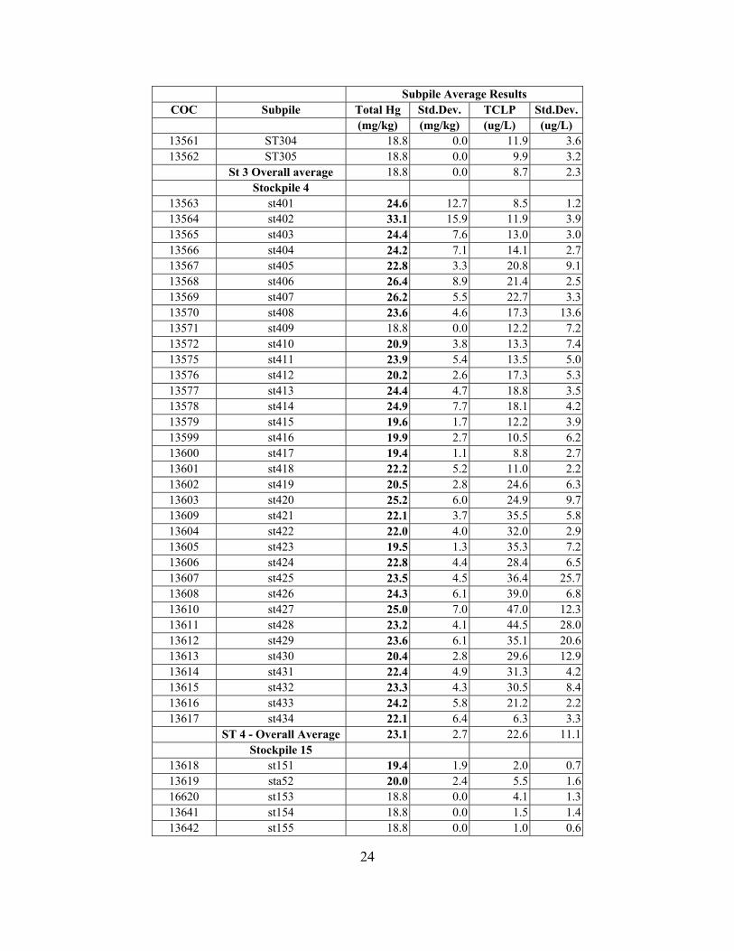
Subpile Average Results COC Subpile Total Hg Std.Dev. TCLP Std.Dev.
(mg/kg) (mg/kg) (ug/L) (ug/L) 13561 ST304 18.8 0.0 11.9 3.6 13562 ST305 18.8 0.0 9.9 3.2
St 3 Overall average 18.8 0.0 8.7 2.3 Stockpile 4
13563 st401 24.6 12.7 8.5 1.2 13564 st402 33.1 15.9 11.9 3.9 13565 st403 24.4 7.6 13.0 3.0 13566 st404 24.2 7.1 14.1 2.7 13567 st405 22.8 3.3 20.8 9.1 13568 st406 26.4 8.9 21.4 2.5 13569 st407 26.2 5.5 22.7 3.3 13570 st408 23.6 4.6 17.3 13.6 13571 st409 18.8 0.0 12.2 7.2 13572 st410 20.9 3.8 13.3 7.4 13575 st411 23.9 5.4 13.5 5.0 13576 st412 20.2 2.6 17.3 5.3 13577 st413 24.4 4.7 18.8 3.5 13578 st414 24.9 7.7 18.1 4.2 13579 st415 19.6 1.7 12.2 3.9 13599 st416 19.9 2.7 10.5 6.2 13600 st417 19.4 1.1 8.8 2.7 13601 st418 22.2 5.2 11.0 2.2 13602 st419 20.5 2.8 24.6 6.3 13603 st420 25.2 6.0 24.9 9.7 13609 st421 22.1 3.7 35.5 5.8 13604 st422 22.0 4.0 32.0 2.9 13605 st423 19.5 1.3 35.3 7.2 13606 st424 22.8 4.4 28.4 6.5 13607 st425 23.5 4.5 36.4 25.7 13608 st426 24.3 6.1 39.0 6.8 13610 st427 25.0 7.0 47.0 12.3 13611 st428 23.2 4.1 44.5 28.0 13612 st429 23.6 6.1 35.1 20.6 13613 st430 20.4 2.8 29.6 12.9 13614 st431 22.4 4.9 31.3 4.2 13615 st432 23.3 4.3 30.5 8.4 13616 st433 24.2 5.8 21.2 2.2 13617 st434 22.1 6.4 6.3 3.3
ST 4 - Overall Average 23.1 2.7 22.6 11.1 Stockpile 15
13618 st151 19.4 1.9 2.0 0.7 13619 sta52 20.0 2.4 5.5 1.6 16620 st153 18.8 0.0 4.1 1.3 13641 st154 18.8 0.0 1.5 1.4 13642 st155 18.8 0.0 1.0 0.6
24

Subpile Average Results COC Subpile Total Hg Std.Dev. TCLP Std.Dev.
(mg/kg) (mg/kg) (ug/L) (ug/L) 13643 st156 18.8 0.0 3.2 1.3 13644 st157 18.8 0.0 2.4 2.6 13645 st158 18.8 0.0 3.6 4.5 13646 st159 18.8 0.0 0.6 0.3 13647 st1510 36.2 31.3 20.3 22.7 13648 st1511 18.8 0.0 1.7 0.3 13649 st1512 27.7 0.0 1.5 0.4 13650 st1513 27.7 0.0 1.5 0.5 13651 st1514 29.1 3.0 4.1 6.6
St 15 Overall Average 22.2 5.6 3.8 5.0 Stockpile 12
13652 st1201 54.6 4.1 32.3 13.4 13653 st1202 53.9 3.9 39.2 13.8 13654 st1203 54.3 7.2 53.4 23.5 13655 st1204 56.4 8.3 102.4 96.7 13656 st1205 61.3 17.6 84.2 28.6 13657 st1206 54.1 8.8 34.2 14.6 13658 st1207 51.3 1.8 25.0 9.2 13739 st1208 51.2 1.8 43.7 7.0 13740 st1209 51.1 1.8 94.7 57.1 13741 st1210 53.3 4.0 57.4 14.4 13742 st1211 52.2 3.7 80.5 13.0 13743 st1212 64.4 20.6 80.0 11.8 13744 st1213 59.7 10.0 84.4 17.0 13745 st1214 60.8 10.9 60.8 9.2 13746 st1215 61.1 4.7 68.4 13.6 13749 st1216 59.0 12.4 70.5 24.3 13750 st1217 56.7 5.5 153.7 196.0 13751 st1218 60.7 9.0 85.2 19.0 13752 st1219 56.4 5.4 88.0 25.9 13753 st1220 53.9 4.0 89.2 83.0 13754 st1221 51.3 2.3 62.8 12.2 13755 st1222 54.4 6.2 56.0 14.0 13756 st1223 56.2 5.8 52.2 18.5 13757 st1224 57.2 4.7 52.7 8.5 13758 st1225 60.0 8.7 67.5 27.6 14315 st1226 68.7 6.9 98.4 36.3 14316 st1227 69.5 12.1 103.0 16.8 14317 st1228 72.6 11.1 112.8 14.2 14318 st1229 76.0 14.9 122.5 27.3 14319 st1230 82.7 20.2 83.0 18.4 14320 st1231 70.1 15.5 26.3 15.5
St 12 Overall Average 59.5 7.9 73.0 29.6 Stockpile 11
25

Subpile Average Results COC Subpile Total Hg Std.Dev. TCLP Std.Dev.
(mg/kg) (mg/kg) (ug/L) (ug/L) 14322 st1101 50.5 0.0 20.7 4.6 14323 st1102 50.9 1.2 26.2 3.1 14324 st1103 55.7 8.8 28.6 7.5 14325 st1104 52.1 2.3 29.8 7.9 14326 st1105 59.7 13.9 43.8 9.8 14327 st1106 57.1 6.1 46.6 18.2 14328 st1107 55.7 6.7 40.5 12.3 14329 st1108 54.9 4.3 23.9 3.7 14330 st1109 51.7 3.2 39.0 12.4 14331 st1110 56.9 4.9 33.3 23.1 14332 st1111 54.5 5.7 30.7 5.9 14333 st1112 51.8 3.3 30.9 6.3 14334 st1113 51.2 1.8 30.7 9.5 14341 st1114 53.9 6.9 27.7 3.8 14342 st1115 51.7 2.3 49.7 23.7 14343 st1116 52.5 5.2 30.3 8.1 14344 st1117 52.5 3.6 30.3 6.0 14345 st1118 53.5 5.2 29.9 6.0 14346 st1119 59.1 16.4 24.8 12.7 14347 st1120 53.0 2.6 48.0 23.7 14348 st1121 52.3 3.1 26.9 11.2 14349 st1122 56.5 10.0 22.1 15.8 14587 st1123 51.7 3.2 21.2 5.9 14588 st1124 58.1 15.6 16.8 5.7 14589 st1125 51.7 2.2 20.8 9.6 14590 st1126 53.5 2.9 26.7 6.2 14591 st1127 52.1 3.3 66.2 67.9 14592 st1128 51.2 1.4 39.7 11.0 14593 st1129 54.5 6.2 32.6 17.9 14594 st1130 51.9 4.2 32.3 8.6 14595 st1131 59.5 9.2 61.5 58.8 14596 st1132 53.5 4.5 40.6 7.8 14597 st1133 56.6 9.4 42.0 6.8 14599 st1134 53.3 3.0 17.1 3.2 14601 st1135 59.6 9.5 75.8 6.2 14602 st1136 54.5 5.5 50.4 10.6 14603 st1137 56.9 5.2 49.2 6.5 14604 st1138 55.4 5.5 31.4 5.5 14605 st1139 57.1 10.1 76.3 16.9 14606 st1140 62.7 11.7 54.6 8.9 14607 st1141 57.3 9.0 63.4 12.3 14608 st1142 59.7 22.3 28.9 5.7 14609 st1143 59.8 10.6 113.4 120.6 14610 st1144 56.7 10.9 63.2 14.5 14611 st1145 55.6 5.6 47.4 19.8
26

Subpile Average Results COC Subpile Std.Dev. TCLP Std.Dev.
(mg/kg) (mg/kg) (ug/L) Total Hg
(ug/L) 14612 st1146 59.2 3.9 43.3 6.7 14613 st1147 58.0 9.8 29.9 4.2 14614 st1148 55.0 5.2 38.8 12.9 14615 st1149 76.1 18.4 72.3 14.8 14616 st1150 55.3 5.8 47.4 28.5 14617 st1151 55.4 6.1 38.7 14.2 14644 st1152 64.1 20.1 29.9 3.9 14645 st1153 53.0 4.1 22.8 3.1 14646 st1154 52.0 2.4 26.4 4.8 14647 st1155 51.6 2.4 34.0 4.8 14648 st1156 58.4 10.6 37.0 8.1 14649 st1157 64.2 19.0 45.3 12.0 14650 st1158 53.1 3.4 36.6 2.6 14651 st1159 53.4 4.0 37.8 5.5 14652 st1160 50.5 0.0 35.3 5.0 14653 st1161 56.3 10.0 23.2 5.7 14654 st1162 53.1 4.7 33.6 4.0 14655 st1163 50.5 0.0 18.4 6.7 14656 st1164 50.5 0.0 8.8 1.5 14657 st1165 50.7 0.8 18.0 3.8
St 11 Overall average 55.2 4.3 37.9 17.5 Stockpile 7
14659 st701 66.9 9.2 6.0 3.2 14660 st702 63.8 10.5 13.6 17.7 14661 st703 68.1 5.9 3.5 5.1 14662 st704 64.2 7.4 4.9 4.5 14663 st705 60.6 8.6 6.1 3.6 14677 st706 66.6 9.4 5.3 2.7 14678 st707 68.3 4.5 11.2 4.2 14679 st708 62.6 8.7 5.4 4.8
St 7 Overall average 65.1 2.8 7.0 3.5 Stockpile 6A 14680 st6A01 50.5 0.0 1.3 0.5 14681 st6A02 50.5 0.0 4.3 4.1 14682 st6A03 51.3 2.5 10.7 17.3 14683 st6A04 52.4 3.9 4.5 4.1 14684 st6A05 52.6 5.7 4.1 1.2 14685 st6A06 52.4 4.5 4.4 3.1 14686 st6A07 53.2 3.9 3.5 0.9 14687 st6A08 53.0 2.8 5.6 2.6 14688 st6A09 50.7 0.4 5.1 1.6 14689 st6A10 54.5 9.2 7.3 9.3 14690 st6A11 53.3 4.5 6.2 1.7 14691 st6A12 52.3 3.4 6.1 2.0 14692 st6A13 52.5 2.9 5.0 3.0
27

Subpile Average Results COC Subpile Std.Dev. TCLP Std.Dev.
(mg/kg) (mg/kg) (ug/L) Total Hg
(ug/L) 14693 st6A14 51.7 1.4 2.5 0.7 14694 st6A15 52.5 3.1 2.4 1.0 14695 st6A16 50.5 0.0 1.2 1.1 14776 st6A17 52.0 3.0 1.2 1.4 14777 st6A18 50.5 0.0 1.0 0.8 14778 st6A19 50.7 0.5 0.9 0.3 14779 st6A20 53.9 4.6 1.2 0.5 14780 st6A21 51.2 1.3 0.9 0.2 14781 st6A22 52.5 4.2 3.2 1.6 14782 st6A23 52.7 3.7 1.4 1.4 14783 st6A24 50.8 0.9 1.3 0.4 14784 st6A25 50.5 0.2 1.2 0.8 14785 st6A26 51.0 1.5 1.3 0.3 14786 st6A27 51.9 3.1 0.8 0.3 14787 st6A28 50.5 0.0 0.7 0.7 14788 st6A29 50.6 0.2 0.6 0.1 14789 st6A30 51.2 1.2 0.8 0.4 St 6A Overall Average 51.8 1.1 3.0 2.5 Stockpile 6C
14872 st6C01 50.8 0.8 2.3 2.1 14874 st6C02 51.5 2.8 3.2 1.1 14875 st6C03 50.5 0.0 7.3 2.5 14876 st6C04 51.6 2.8 19.3 32.6 14877 st6C05 51.2 1.7 3.3 1.3 14878 st6C06 50.5 0.0 15.9 37.6 14880 st6C07 51.6 2.5 7.2 11.0 14881 st6C08 61.1 15.3 8.9 11.6 14882 st6C09 86.6 36.4 18.2 2.8 14883 st6C10 69.6 11.2 10.3 3.1
St 6C Overall average 57.5 12.0 9.6 6.3 Stockpile 6R
14884 st6R01 55.6 4.6 4.0 2.9 14885 st6R02 53.8 5.1 5.3 3.5 14886 st6R03 53.8 4.7 10.7 15.4 14887 st6R04 59.4 8.8 5.5 1.3 14905 st6R05 52.7 3.0 2.5 2.0 14906 st6R06 52.9 5.7 6.6 2.1 14907 st6R07 55.6 5.5 8.6 4.8 14909 st6R08 55.6 6.8 7.1 4.0 14910 st6R09 83.2 27.6 52.4 45.1 14911 st6R10 69.0 7.1 36.6 14.9 14912 st6R11 59.6 8.6 12.8 2.6 14913 st6R12 67.9 7.6 19.6 19.5 14914 st6R13 62.7 9.7 16.7 9.4 14915 st6R14 59.3 8.1 27.2 13.5
28

Subpile Average Results COC Subpile Std.Dev. TCLP Std.Dev.
(mg/kg) (mg/kg) (ug/L) Total Hg
(ug/L) 14916 st6R15 61.6 12.6 10.3 3.0 14917 st6R16 51.9 2.7 21.5 14.5 14918 st6R17 58.5 11.2 44.2 11.7 14919 st6R18 59.3 11.8 22.8 5.4 14920 st6R19 59.9 5.8 23.9 9.2 14921 st6R20 56.0 6.6 12.5 7.6 14922 st6R21 59.1 10.3 18.5 3.2 14923 st6R22 59.6 6.5 15.3 4.3 14924 st6R23 59.9 10.8 24.4 6.8 14985 st6R24 73.7 8.3 37.3 43.1 14986 st6R25 59.6 6.7 20.2 9.6 14987 st6R26 53.4 2.8 33.5 21.8 14988 st6R27 55.9 4.9 23.6 25.0 14989 st6R28 58.3 13.2 7.2 5.2 14990 st6R29 58.1 4.3 63.7 111.2 14991 st6R30 53.4 5.0 32.7 45.9 14992 st6R31 61.8 11.4 16.2 3.4 15406 st6R32 61.6 8.1 25.8 11.0 15407 st6R33 59.3 5.6 97.1 228.2 15408 st6R34 61.1 18.9 19.8 16.6 15409 st6R35 51.2 2.2 16.9 7.9 15410 st6R36 56.0 6.8 13.8 5.4 15411 st6R37 53.4 4.3 15.0 19.0 15412 st6R38 57.1 6.0 11.0 3.2 15413 st6R39 54.2 4.0 8.0 0.7 15414 st6R40 55.9 4.3 7.1 1.0 15415 st6R41 56.2 5.3 5.8 1.3 15416 st6R42 50.5 0.0 4.2 1.3 15418 st6R43 58.7 6.0 11.6 6.2 15419 st6R44 51.1 1.3 16.3 8.8 15420 st6R45 50.8 0.6 21.0 10.0 15421 st6R46 54.2 5.4 21.4 4.5 15422 st6R47 63.2 22.7 35.9 14.1 15423 st6R48 56.9 11.9 53.2 62.9 15424 st6R49 68.6 10.3 77.9 39.6 15425 st6R50 51.5 2.0 30.9 6.3 15426 st6R51 50.5 0.0 120.7 312.1 15417 st6R52 52.7 3.2 5.8 2.0 15427 st6R53 54.0 4.8 3.4 1.8
ST 6R Overall Average 57.9 6.1 23.9 23.3
29

Table 5 TCLP Mercury Results for Common Data Points
ASTD Field Lab Hits Contract Lab
Stockpile # of Data Average Std. >100 ppb Average Std. # Points µg/L Dev. 95%* F-lab Con µg/L Dev. 95%*3 6 9.1 4.8 18.7 0 0 7.2 4.3 15.94 14 19.2 10.2 39.6 0 0 11.3 4.9 21.26a 13 3.5 5.0 13.5 0 0 3.0 2.6 8.26R 22 20.7 19.8 60.3 0 1 40.7 42.0 124.76C 3 3.6 1.5 6.6 0 0 12.3 10.1 32.47 4 2.4 1.6 5.6 0 1 97.6 179.7 457.08 41 7.4 8.5 24.4 0 0 5.1 2.1 9.3
11 25 31.8 12.3 56.4 0 2 45.6 33.5 112.712 13 71.1 26.6 124.3 3 1 51.8 31.3 114.315 3 2.7 2.1 6.9 0 0 4.1 5.1 14.3
* Refers to the 95% confidence value, calculated as [Average + (2 x Std.Dev.)]
Table 6 TCLP Mercury Results Comparison for All Data Points
ASTD Field Lab Hits Contract Lab
Stockpile Average Std. # of Data >100 ppb Average Std. # of Data# µg/L Dev. 95%* Points F-lab Con µg/L Dev. 95%* Points 3 8.8 3.7 16.2 42 0 0 7.2 4.3 15.9 6 4 22.6 14.2 51.1 286 0 0 11.3 4.9 21.2 14 6a 3.1 4.5 12.0 251 10 0 3.0 2.6 8.2 13 6R 24.2 4.5 33.2 443 10 1 40.7 42.0 124.7 22 6C 9.5 16.5 42.6 83 1 0 12.3 10.1 32.4 3 7 7.0 7.5 22.1 66 0 1 79.3 161.0 401.2 5 8 10.7 9.1 28.9 322 0 0 5.7 2.4 10.5 103
11 37.7 32.2 102.1 545 8 2 45.6 33.5 112.7 25 12 72.5 51.5 175.5 260 42 1 51.8 31.3 114.3 13 15 4.2 9.0 22.3 117 0 1 7.3 5.9 19.0 5 all 27.2 34.8 96.9 2415 71 6 16.7 34.4 85.4 209
* Refers to the 95% confidence value, calculated as [Average + (2 x Std.Dev.)]
30
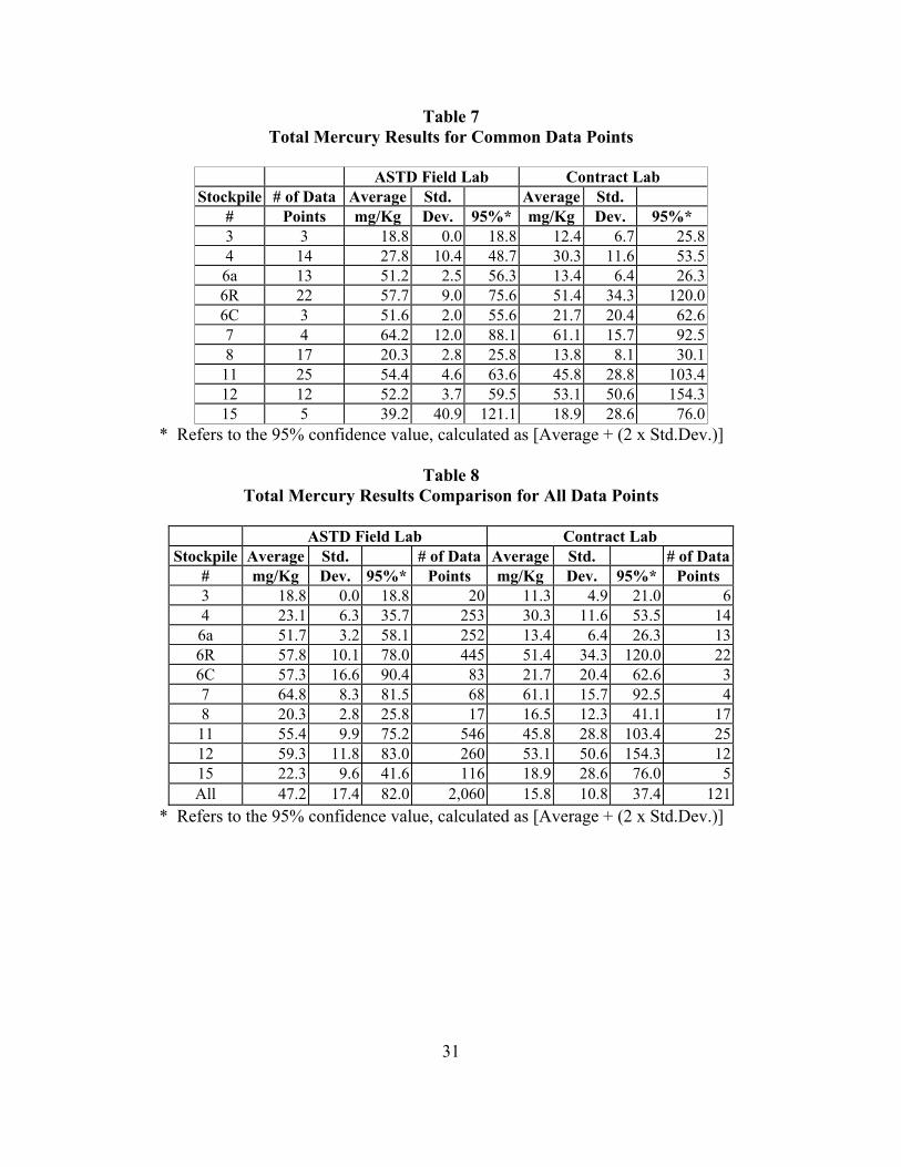
Table 7 Total Mercury Results for Common Data Points
ASTD Field Lab Contract Lab
Stockpile # of Data Average Std. Average Std. # Points mg/Kg Dev. 95%* mg/Kg Dev. 95%* 3 3 18.8 0.0 18.8 12.4 6.7 25.8 4 14 27.8 10.4 48.7 30.3 11.6 53.5 6a 13 51.2 2.5 56.3 13.4 6.4 26.3 6R 22 57.7 9.0 75.6 51.4 34.3 120.0 6C 3 51.6 2.0 55.6 21.7 20.4 62.6 7 4 64.2 12.0 88.1 61.1 15.7 92.5 8 17 20.3 2.8 25.8 13.8 8.1 30.1
11 25 54.4 4.6 63.6 45.8 28.8 103.4 12 12 52.2 3.7 59.5 53.1 50.6 154.3 15 5 39.2 40.9 121.1 18.9 28.6 76.0
* Refers to the 95% confidence value, calculated as [Average + (2 x Std.Dev.)]
Table 8 Total Mercury Results Comparison for All Data Points
ASTD Field Lab Contract Lab
Stockpile Average Std. # of Data Average Std. # of Data# mg/Kg Dev. 95%* Points mg/Kg Dev. 95%* Points 3 18.8 0.0 18.8 20 11.3 4.9 21.0 64 23.1 6.3 35.7 253 30.3 11.6 53.5 146a 51.7 3.2 58.1 252 13.4 6.4 26.3 136R 57.8 10.1 78.0 445 51.4 34.3 120.0 226C 57.3 16.6 90.4 83 21.7 20.4 62.6 37 64.8 8.3 81.5 68 61.1 15.7 92.5 48 20.3 2.8 25.8 17 16.5 12.3 41.1 17
11 55.4 9.9 75.2 546 45.8 28.8 103.4 2512 59.3 11.8 83.0 260 53.1 50.6 154.3 1215 22.3 9.6 41.6 116 18.9 28.6 76.0 5All 47.2 17.4 82.0 2,060 15.8 10.8 37.4 121
* Refers to the 95% confidence value, calculated as [Average + (2 x Std.Dev.)]
31

32
Appendices (On Compact Disc)
1. In-Situ Object Counting System (ISOCS) – Gamma Spectroscopy Data Summaries 2. ASTD Field Lab – Total Mercury and TCLP Mercury Data 3. QA Data – Comparisons with Off-site Lab results