nano-engineering of high harmonic generation in solid state …€¦ · standing of the ultrafast...
TRANSCRIPT

Nano-engineering of High Harmonic Generation in SolidState Systems
ByShaimaa Almalki
A thesis submitted to the Faculty of Graduate and PostdoctoralStudies in partial fulfilment of the requirements for the degree of
Doctorate of Philosophy in Physics
Department of PhysicsFaculty of Science
University of Ottawa
c© Shaimaa Almalki, Ottawa, Canada, 2019

List of Publications
1. S Almalki, AM Parks, G Bart, PB Corkum, T Brabec, and CR McDonald.High harmonic generation tomography of impurities in solids: Conceptual anal-ysis. Physical Review B, 98(14):144307, 2018.
2. S Almalki, AM Parks, T Brabec, and CR McDonald. Nanoengineering ofstrong field processes in solids. Journal of Physics B: Atomic, Molecular andOptical Physics, 51(8):084001, 2018.
3. CR McDonald, KS Amin, S Almalki, and T Brabec. Enhancing high har-monic output in solids through quantum confinement. Physical review letters,119(18):183902, 2017.
ii

Contents
List of Figures vii
Abstract viii
Acknowledgements x
Introduction 1
1 Harmonic generation in gas phase 51.1 Low-harmonic generation . . . . . . . . . . . . . . . . . . . . . . . . 5
1.1.1 Time-dependent perturbation theory . . . . . . . . . . . . . 61.1.2 The breakdown of perturbation theory . . . . . . . . . . . . 7
1.2 High-harmonic generation . . . . . . . . . . . . . . . . . . . . . . . 91.2.1 Semiclassical approach . . . . . . . . . . . . . . . . . . . . . 91.2.2 Quantum approach . . . . . . . . . . . . . . . . . . . . . . . 13
1.3 Phase matching . . . . . . . . . . . . . . . . . . . . . . . . . . . . . 151.4 HHG tomography . . . . . . . . . . . . . . . . . . . . . . . . . . . . 16
2 High harmonic generation in solids 192.1 Distinction from atoms . . . . . . . . . . . . . . . . . . . . . . . . . 192.2 The nonlinearity of band velocity . . . . . . . . . . . . . . . . . . . 212.3 Theory of HHG in solids . . . . . . . . . . . . . . . . . . . . . . . . 22
2.3.1 Solution of the time-dependent Schrodinger equation . . . . 222.3.2 Semiclassical model for semiconductor HHG . . . . . . . . . 252.3.3 Effect of dephasing on interband vs intraband harmonics . . 26
3 HHG in Low-Dimensional Solid State Systems 283.1 Quantum confinement . . . . . . . . . . . . . . . . . . . . . . . . . 283.2 Quantum confinement role in enhancing HHG . . . . . . . . . . . . 293.3 Methods . . . . . . . . . . . . . . . . . . . . . . . . . . . . . . . . . 31
iii

3.3.1 Model for confined quantum systems . . . . . . . . . . . . . 313.3.2 Ionization dynamics and high harmonic generation . . . . . 33
3.4 Results and Discussion . . . . . . . . . . . . . . . . . . . . . . . . . 363.4.1 Ionization and harmonic output . . . . . . . . . . . . . . . . 363.4.2 The effect of confinement on diffusion and recollision . . . . 40
3.5 Summary . . . . . . . . . . . . . . . . . . . . . . . . . . . . . . . . 43
4 Impurity Tomography 444.1 HHG in doped semiconductors . . . . . . . . . . . . . . . . . . . . . 44
4.1.1 Quantum mechanical model . . . . . . . . . . . . . . . . . . 464.1.2 Derivation of the ground state for a shallow impurity . . . . 474.1.3 Solution of the time-dependent Schrodinger equation . . . . 494.1.4 Semicalssical model for impurity high-harmonic generation . 52
4.2 Numerical details . . . . . . . . . . . . . . . . . . . . . . . . . . . . 534.3 Tomographic reconstruction of the impurity state . . . . . . . . . . 554.4 Dimensionality considerations for tomographic reconstruction . . . . 584.5 Summary . . . . . . . . . . . . . . . . . . . . . . . . . . . . . . . . 60
Conclusions 61
A Derivation of transverse population and current 64
B Impurity versus intraband harmonics 70
C Numerical solution of the two-band equations 72
D Atomic units and Conversion Factors 74
Bibliography 82
iv

List of Figures
1.1 The three-step model: (a) tunnel ionization. (b) acceleration. (c)recombination. . . . . . . . . . . . . . . . . . . . . . . . . . . . . . 9
1.2 (a) Electron trajectories in a linearly polarized laser field born atdifferent times. (b) A widened view of (a). . . . . . . . . . . . . . . 11
1.3 (a) Time of birth versus time of return. (b) The kinetic energy of theelectron at the time of return as a function of the birth time. Theshaded region indicate the kinetic energy of long electron trajectories 12
2.1 Diagram of the three-step model in the momentum space for (a) anatom (b) a bulk solid. . . . . . . . . . . . . . . . . . . . . . . . . . . 20
2.2 The Bloch velocity (blue) and the electric field (red). . . . . . . . . 222.3 Harmonic spectra for the interband (blue) and intraband (red) con-
tributions in 1D semiconductor with Eg = 3.3 eV and T2 = 1 fs. Theband structure is given by Eqs. (3.2). The system is exposed to aGaussian pulse of λ0 = 6.4µm at F0 = 0.26 V·A−1 with a FWHM ofthree cycles. . . . . . . . . . . . . . . . . . . . . . . . . . . . . . . . 25
3.1 Schematic depiction of the effect of quantum confinement on wavepacket spreading and interband harmonics; the black circles representelectrons and the grey circles represent holes . . . . . . . . . . . . . 30
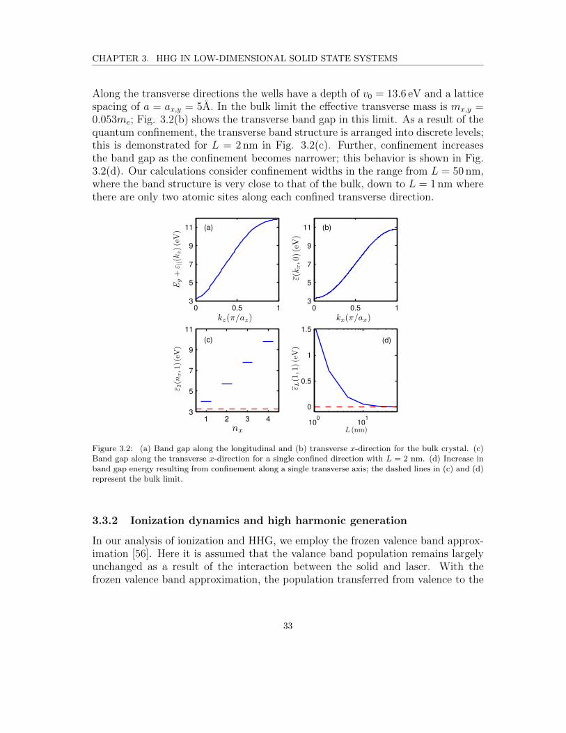
3.2 (a) Band gap along the longitudinal and (b) transverse x-directionfor the bulk crystal. (c) Band gap along the transverse x-directionfor a single confined direction with L = 2 nm. (d) Increase in bandgap energy resulting from confinement along a single transverse axis;the dashed lines in (c) and (d) represent the bulk limit. . . . . . . . 33
3.3 Results for our model system with confinement along two and singletransverse directions. . . . . . . . . . . . . . . . . . . . . . . . . . . 38
3.4 Yield ratio versus confinement width for λ0 = 3.2µm (solid) andλ0 = 6.4µm (dash-dot) for (a) the confinement along both transversedirections and (b) confinement along a single transverse direction. . 39
v

3.5 (a) Ratio of final conduction band population in the 1D system tothe L = 50 nm system (circles with solid line) versus λ0; the dashedline gives (n2D
⊥ )−1 predicted by equation (3.7). (b) Ratio of final con-duction band population in the 2D system to the L = 50 nm system(circles with solid line) versus λ0; the dashed line gives (n1D
⊥ )−1 pre-dicted by equation (3.7). (c) Ratio of harmonic output from the 1Dsystem to the L = 50 nm (solid) and the L = 20 nm (dash-dot) sys-tems versus λ0. The dashed line shows the prediction for |j2D
⊥ |−2 fromequation (3.8). (d) Ratio of harmonic output from the 2D system tothe L = 50 nm (solid) and the L = 20 nm (dash-dot) systems versusλ0. The dashed line shows the prediction for |j1D
⊥ |−2 from equation(3.8). . . . . . . . . . . . . . . . . . . . . . . . . . . . . . . . . . . . 41
4.1 (a) Periodic potential of the unperturbed bulk solid (blue) plus theimpurity potential (red); the shalloe impurity ground state that ex-tends over many lattice cites is represented by the shaded curve. (b)Space representation of the three-step model for HHG from an im-purity. (c) Reciprocal space representation of the three-step modelfor HHG from an impurity. . . . . . . . . . . . . . . . . . . . . . . . 45
4.2 (a) Structure of the conduction band obtained from diagonalizationof the Hamiltonian. (b) Dipole moment calculated using Eq. (4.22). 55
4.3 (a) Birth time t′ (red) and return times t (blue) from the semiclassicaltrajectories versus harmonic order. (b) Ionization rate w ∝ exp
(−
23
√m(2(Eg − ε0))3/2/F (t′)
)versus harmonic order. (c) Propagation
effects α2 ∝ exp(−2(t−t′)/T2
)/(t−t′) versus harmonic order. (d)
Magnitude squared of the dipole moment as a function of harmonicorder (blue); the product of the three pre-exponential terms in Eq.(4.34) represented by blue lines in (b)-(d) is plotted for the short (reddots) and long (green squares) trajectory branches; the magnitude isadapted to match the dipole moment. In (a) - (c) the shaded regionsindicate the contributions from long trajectories. . . . . . . . . . . . 56
4.4 Scaling comparison of the harmonic spectrum (blue) to the dipole(red, dashed); the dipole has been shifted down in order to comparewith the spectrum. The harmonics in the shaded region are thosewhose energy is below Eg − ε0. . . . . . . . . . . . . . . . . . . . . . 57
4.5 Comparison between the impurity ground state (blue, shaded) andthe reconstructed ground state (red). The region between the verticaldashed lines represents 11 unit cells. . . . . . . . . . . . . . . . . . . 58
vi

4.6 Magnitude squared of the dipole moment as a function of harmonicorder (blue); the product of the three pre-exponential terms in Eq.(2.51) of the main manuscript is plotted for the short (red dots) andlong (green squares) trajectory branches for (a) the one-dimensionalsystem and (b) a three-dimensional system. The magnitude of thesemiclassical curves is adapted to match the dipole moment. . . . . 59
B.1 The impurity (blue) and intraband (green) harmonic spectra. Thered, dashed line represents the dipole moment. The shaded areaindicates the below impurity ionization potential region. The dipolehas been shifted on the y-axis to compare with the shape of theharmonic spectra. . . . . . . . . . . . . . . . . . . . . . . . . . . . . 71
vii

Abstract
High harmonic generation (HHG) in solids has two main applications. First, HHGis an all-solid-state source of coherent attosecond very ultraviolet (VUV) radiation.As such, it presents a promising source for attosecond science. The ultimate goalof attosecond science is to make spatially and temporally resolved movies of micro-scopic processes, such as the making and breaking of molecular bonds. Second, theHHG process itself can be used to spatially and temporally resolve fast processes inthe condensed matter phase, such as charge shielding, multi-electron interactions,and the dynamics and decay of collective excitations. The main obstacles to realizethese goals are: the very low efficiency of HHG in solids and incomplete under-standing of the ultrafast dynamics of the complex many-body processes occurringin the condensed matter phase.
The theoretical analysis developed in this thesis promises progress along both di-rections. First, it is demonstrated that nanoengineering by using lower-dimensionalsolids can drastically enhance the efficiency of HHG. The effect of quantum confine-ment on HHG in semiconductor materials is studied by systematically varying theconfinement width along one and two directions transverse to the laser polarization.Our analysis shows growth in high harmonic efficiency concurrent with a reductionof ionization. This decrease in ionization comes as a consequence of an increasedband gap resulting from the confinement. The increase in harmonic efficiency resultsfrom a restriction of wave packet spreading, leading to greater re-collision probabil-ity. Consequently, nanoengineering of one and two-dimensional nanosystems mayprove to be a viable means to increase harmonic yield and photon energy in semi-conductor materials driven by intense laser fields. Thus, it will contribute towardsthe development of reliable, all-solid-state, small-scale, and laboratory attosecondpulse sources.
Second, it is shown that HHG from impurities can be used to tomographicallyreconstruct impurity orbitals. A quasi-classical three-step model is developed thatbuilds a basis for impurity tomography. HHG from impurities is found to be simi-lar to the high harmonic generation in atomic and molecular gases with the maindifference coming from the non-parabolic nature of the bands. This opens a new
viii
avenue for strong field atomic and molecular physics in the condensed matter phaseand allows many of the processes developed for gas-phase attosecond science to beapplied to the condensed matter phase. As a first application, my conceptual studydemonstrates the feasibility of tomographic measurement of impurity orbitals. Ul-timately, this could result in temporally and spatially resolved measurements ofelectronic processes in impurities with potential relevance to quantum informationsciences, where impurities are prime candidates for realizing qubits and single pho-ton sources. Although scanning tunneling microscope (STMs) can measure electroncharge distributions in impurities, measurements are limited to the first few surfacelayers and ultrafast time resolution is not possible yet. As a result, HHG tomogra-phy can add complementary capacities to the study of impurities.
ix

Acknowledgements
All praise the Almighty Allah for giving me the strength and ability to completethis journey.
There are no words that can express my deep gratitude to my brother, Abdull-Rahman, not only for accompanying me but also for all his sacrifices, encourage-ment, and patience. Most of all my appreciation goes to my parents and siblingsfor their unconditional love, endless support, and prayers.
I wish to thank my supervisor, Prof. Thomas Brabec, for giving me the oppor-tunity to be in his research group and for continuous support. I would also like toexpress my thanks to Dr. Chris McDonald for his advice, assistance in keeping myprogress on schedule and helping in numerical analysis. Special thanks to Azza binTaher, the ex-member of our group, for all nights we spent studying together in theoffice.
I would like to thank each of the faculty members who give me the chance tobe a teaching assistant for them: Dr. Michael Wong, Dr. Andrzej Czajkowski, andDr. Peter Piercy.
My sincere thanks are also extended to the Ministry of Education in Saudi Arabiarepresented by the Saudi Arabian Cultural Bureau in Canada for financial support.I owe thanks to my advisors in the bureau, Mrs. Nancy Jad and Dr. Ziyad Jasimfor their insightful advice and constant kindness.
Finally, my grateful thank goes to my friend, Aisha Okmi, for understanding,supporting, and being a good listener whenever I need to babble. Thanks also tomy friend, Norah Alotubi, and her beloved daughter, Dalal, for all great time I havespent with them in Ottawa.
x

Introduction
Nearly a quarter century has passed since the re-collision picture for atomic systemsexposed to intense-laser fields came into focus [1]. In particular, this picture pro-vided a simple mechanism through which the process of high harmonic generation(HHG) could be viewed — the three-step model. Here an electron is (i) brought upinto the continuum, (ii) accelerated away from its parent ion by the electric fieldof the laser and then driven back when the field changes direction, resulting in (iii)re-collision with the parent ion. This re-collision results in the emission of coherentradiation that has a frequency that is many multiples of the driving frequency of thelaser. Ultimately, this understanding led to the emergence of attosecond science [2].As recollision takes place during a fraction of the laser half-cycle, attosecond pulsesare generated. The Holy Grail of attosecond science is to make movies of funda-mental microscopic processes, such as the making and breaking of chemical bonds.HHG takes a central role in attosecond science, as a source for attosecond pulsesand also as a direct measurement method for ultrafast processes. Additional pro-cesses occur during recollision and rescattering [3], such as nonsequential doubleionization, above-threshold ionization, and laser-induced electron diffraction [4–7];these processes also contain structural information and are additional examples ofhow the three-step process of HHG can be used to directly probe ultrafast dynamicsin the matter.
Recent experiments with mid-infrared [8–11] and THz pump sources [12–14] havedemonstrated HHG in solids. The theoretical study has identified two mechanisms[15,16]; (i) intraband HHG due to the non-parabolic nature of bands [9] was foundto be dominant in dielectrics; (ii) interband HHG dominates in semiconductorsand is created in a three-step process similar to atomic and molecular HHG [17].This similarity provides an avenue through which the above-discussed tools andtechniques of attosecond science developed for atomic and molecular systems canbe applied to solid state physics.
There are two main motivations to study HHG in the condensed matter phase.First, an all-solid-state attosecond radiation source is very attractive. Second, sim-
1

INTRODUCTION
ilar to atomic and molecular gases, there are ultrafast and ultrafine processes insolids that can be resolved with HHG directly or with attosecond pulses. The mainobstacles to achieving these goals are a too low HHG efficiency in solids and a farfrom complete theoretical understanding of the dynamic interaction of intense laserfields with solids. One of the advantages to working with solids over atomic gases isthat the properties of solids can be changed by doping, reducing dimensionality andaltering the morphology of the material. Recently, HHG in two-dimensional solidshas been experimentally demonstrated [18]. In addition, HHG involving solid statesystems with impurities has been considered [19, 20]. The goal of this dissertationis to extend our theory knowledge from HHG in solids to HHG in nano-engineeredsystems, such as low-dimensional solids and impurity doped materials. In the firstpart of the thesis, strong field physics and HHG in low dimensional systems suchas quantum wires and quantum sheets will be investigated. In the second part, thetheory of HHG in bulk semiconductors with shallow donor states is developed andapplied to study the tomographic reconstruction of impurity orbitals from harmonicspectra. Thus, my thesis contributes to the two main motivations outlined above,as will be explained in more detail in the remainder of this section.
For HHG, in both atoms and solids, to be viable for attosecond applications, theamount of harmonic output and the maximum photon energy that can be producedmust be considered. To understand the limitations, HHG has to be considered froma microscopic (single atom in laser) and a macroscopic (wave propagation in atomicgas) viewpoint. Both parts underlie different limitations. The microscopic efficiencyis determined by the amount of ionization per laser half cycle and the part of the freeelectron wavepacket that recombines with the parent ion during recollision. Recom-bination is strongly influenced by quantum diffusion, i.e. the electron wavepacketborn by tunnel ionization spreads during its excursion in the continuum. Once itrecollides with the parent ion, only a tiny fraction of the wavepacket overlaps withthe parent ion ground state, resulting in low quantum efficiencies. Quantum dif-fusion grows in strength with increasing excursion amplitude which increases withhigher pump laser intensity and longer wavelength. Quantum diffusion presents afundamental limitation in both gases and solids.
The macroscopic component of HHG is limited by phase mismatch between pumplaser and harmonic beam and by reabsorption of harmonic radiation. Reabsorptionin gases does not play a dominant role due to their comparatively low atom density(up to 1019 atoms/cm3). HHG in gases is dominantly limited by phase mismatchdue to the different refractive indices experienced by the pump laser and harmonicsignal. By contrast, reabsorption is the dominant limiting mechanism in solids dueto the significantly higher densities, and phase mismatch does not play any role.
What has so far been done to increase harmonic pulse and photon energies?
2

INTRODUCTION
One method of obtaining higher photon energies is to increase the peak field inten-sity and/or wavelength of the driving laser. Whether the harmonic pulse energyincreases with increasing laser intensity is a more subtle question and has to betreated on a case by case basis. There is a limit to how much the pump laser in-tensity and therewith harmonic photon energy can be increased. In gases, it is setby the depletion of ionization, whereas in solids is determined by the onset of ma-terial damage. Increase in pump wavelength results in longer excursion amplitudesand stronger quantum diffusion resulting in a reduction of harmonic efficiency. Ithas been demonstrated that by confining the system transversely with a magneticfield HHG in gases can be increased [21]. However, so far the effects of quantumdiffusion have turned out to be very difficult to compensate for. Quantum diffusionalso limits interband HHG in solids [15, 16]. HHG in semiconductors requires lowwavelength pulse lasers in the mid-infrared wavelength regime. The resulting largeelectron excursion amplitude results in strong quantum spreading of the electronwavepacket and small recollision probabilities.
Various phase matching methods have been developed for HHG in gases. Theywork well for individual narrow band harmonics, however are difficult to realize overthe wide spectrum of attosecond pulses. In solids, harmonic propagation is domi-nated by absorption losses from deeper bound core-level electrons; phase mismatcheffects can be neglected. So far, no remedy has been found for absorption losses. Inthe condensed matter phase, quantum diffusion and absorption losses are the twomain limiting effects of HHG.
One of the main findings of my thesis is that recollision and thus HHG can beincreased in low dimensional quantum systems. The effect of quantum confinementalong one or two transverse directions will restrict the motion of carriers alongthese directions. This, in turn, restricts quantum diffusion and reduces wave packetspreading during the quiver motion of the electron-hole pair, leading to a moresignificant recollision cross-section. Potentially, stacked lower dimensional systems,such as a quantum wire forest, might also contribute to lifting the second limita-tion. In such systems, harmonics are generated in the low-dimensional material,however propagation occurs also in the gaps between the material layers, where noreabsorption exists. This point will be subject to further research. The first partof my thesis contributes to enhancing high harmonic efficiency in solids bringing uscloser to efficient all-solid-state table top attosecond sources.
As the physical pictures of HHG in gases and semiconductors are very similar,the hope is that attosecond technology can be transferred from gases to the solidstate phase. One such example is the second major result of my thesis. It con-tributes to the second motivation point discussed above. The potential of applyingmolecular HHG tomography [22–24] to impurities is studied here. High harmonic
3

INTRODUCTION
emission is considered directly from the impurity under a THz driving field. Be-cause of the similarity between HHG in atoms and impurities, gas phase techniquescan be translated into the condensed matter phase. Our result shows that HHGcan be directly used as a spectroscopic method to resolve ultrafast processes involv-ing impurities. As an example, tomographic reconstruction of the impurity groundstate is demonstrated in a 1D model system. The impurity dipole moment is foundto be the dominant factor in determining the magnitude of the harmonic signal asa function of harmonic order; ionization and propagation which have to be factoredout in molecular tomography play a lesser role here. This indicates substantial fa-cilitation due to the potential for direct reconstruction of the impurity ground statefrom the harmonic spectrum. High harmonic generation has been the bedrock onwhich attosecond spectroscopy techniques in gases have been built. These tech-niques have allowed for the study of the temporal and structural characteristics ofatomic and molecular systems [25–28]. My thesis continues this work from the gasto the condensed matter phase.
The thesis is structured as follows. Chapter 1 is part of the introduction; thetheory of high harmonic generation in atoms is introduced in more detail. In chapter2, the theory of HHG in bulk solids is presented. The novel results are presentedin chapters 3 and 4. The theoretical analysis of HHG in model nanostructures isintroduced in chapter 3. The study of HHG from impurity ground state and thereconstruction of its wave function are shown in chapter 4.
All work presented here has been already published in the papers mentionedabove in the list of publications. The theory of using nanowire to enhance theharmonic output was developed by T. Brabec and CR. McDonald. I worked onsimulations and analysis of results and worked on the paper. I also made the maincontributions to generalizing the results to thin layers in paper 2. In paper 3, I wasthe main researcher and was supported by T. Brabec and CR. McDonald to achievethe presented results.
4

Chapter 1
Harmonic generation in gas phase
In 1987, McPherson et al. [29] were the first to observe the harmonic spectrumgenerated from rare gases by intense ultraviolet (248 nm) radiation (1015 − 1016
W/cm2). The expectation at that time was to obtain an exponentially decreasingspectrum with harmonic orders. However, their unexpected result showed a har-monic spectrum that exponentially decreases at low order harmonics followed bya plateau that expands over several harmonic orders with approximately constantharmonic intensity. Then, there was a drop off region where the harmonic spectralintensity dramatically falls off. The interpretation of this behavior was given clas-sically by Corkum et al. [1] and quantum mechanically by Lewenstein et al. [30] afew years later.
The goal of this chapter is to give a brief description of high harmonic generationand highlight the physics behind the three regions of its spectrum which are low-order harmonics, plateau, and cutoff.
1.1 Low-harmonic generation
When a conventional crystal medium is exposed to sufficiently high laser intensities,harmonics of the fundamental laser field can be generated. The phenomenon wasfirst demonstrated by Franke et al. in 1961 [31]. The demonstration synchronizedwith the development of the laser, which created the required high-intensity coherentlight. The production of harmonics is attributed to the laser-induced polarizationof the medium P(t) which has nonlinear dependence on the laser field F(t). Theresponse of the medium is given by
P(t) = ε0(χ(1)F(t) +
∑j>1
χ(j)Fj(t)), (1.1)
5
CHAPTER 1. HARMONIC GENERATION IN GAS PHASE
where χ is the electric susceptibility and ε0 is the permittivity of free space. The firstterm in Equation (1.1) represents the linear polarization response. Other nonlinearterms become significant when the laser field strength roughly ranges between 108
to 1013 W/cm2 [32]. Note that even-nonlinear processes cannot appear in a cen-trosymmetric material due to the inversion symmetry of the polarization and laserelectric field. For such systems, only odd terms show up [33].
For simplicity’s sake, the particle nature of the electron is usually used to describethe generation process. An electron jumps to higher real or virtual energy level bystimulated absorption. If the electron absorbs q photons from the laser field offrequency ω0, it emits a single photon with qω0 energy as it decays to its initialenergy level. The output field intensity relies on the probability of having q-photontransitions, and it is proportional to the square of the atomic number density.Therefore, a high-intensity field can be achieved when the response of each atomconstructively interferes which implies that the momentum is conserved. In otherwords, the phase-matching condition must be fulfilled, see Section 1.3.
1.1.1 Time-dependent perturbation theory
This approach is mainly based on treating the effects of the laser field on a quantumsystem as a perturbation. The following derivation is given in Refs. [34] and [33].Here and throughout the rest of the thesis, the atomic units are used unless other-wise indicated, see Appendix D.
The Hamiltonian of the system in length gauge is assumed to be
H = H0 + λH ′, (1.2)
where H0 = −12∇2 + V (r) is the Hamiltonian of the atom before the presence of
the laser field, λ is a small parameter, and H ′ = −x · F(t) = −xF0eiω0t is the
interaction Hamiltonian. Let |ψ(0)n (t)
⟩= e−iωnt|φ(0)
n
⟩be the eigenstates of H0 with
eigenvalues En = ωn. The perturbed states can be expanded as in terms of |ψ(0)n (t)
⟩with probability amplitudes al(t) as
|ψn(t)⟩
=∑l
al(t)|ψ(0)n (t)
⟩=∑l
al(t)e−iωnt|φ(0)
n
⟩, (1.3)
where the probability amplitudes can be expressed as a sum of different order cor-rection as
al(t) =∑m
λma(m)l (t) (1.4)
6

CHAPTER 1. HARMONIC GENERATION IN GAS PHASE
Substituting Eq.(1.3) into time-dependent Schrodinger equation and multipling
both sides by eiωkt⟨φ
(0)k | gives the rate of probability amplitudes
i∂ta(m)k (t) = −F0
∑l
a(m−1)l xkle
iωklt, (1.5)
where xkl =⟨φ
(0)k |x|φ
(0)n
⟩is the dipole transition matrix and ωkl = ωk −ωl−ω0. To
find a(m)k , one needs to find the the amplitude a
(m−1)l which is also defined by a
(m−2)p .
However, if a(m−2)p is small compared to a
(m−1)l , then the integration of a
(m−1)l can
be approximated to
a(m−1)l = F0
∑p
a(m−2)p xlpe
iωlp
ωlp. (1.6)
Using Eq.(1.6) to rewrite Eq.(1.5) leads to
i∂ta(m)k (t) = −(F0)2
∑l,p
a(m−2)p xklxlp
ωlpei(ωk−ωp−2ω0)t. (1.7)
One still needs to find a(m−2)p , etc. Let us assume the transition from state l to state
k is non-resonant and it occurs via intermidate states, l1, l2, ..., lm−2, lm−1. Eachtransition between these intermidiate states is a single-photon transition thereforethe mth-order of ak can be written as
i∂ta(m)k (t) = −(F0)m
l∑lm−1,lm−2,...
xklm−1xlm−1lm−2 · · ·xl1lωklm−1ωlm−1lm−2 · · ·ωl2l1
ei(ωk−ωl−mω0)t. (1.8)
Equation (1.8) represents a perturbative m-photon transition rate. The transitionrate of population is then proportional to (Im):
Γ(m) ∝ Im. (1.9)
Therefore, the probability of this process diminishes with the number of photonsneeded to excite the electron.
1.1.2 The breakdown of perturbation theory
The linear and lowest nonlinear orders of the probability amplitude can be deducedfrom Eq. (1.8). The evaluation of the integral gives
a(1)k (t) = F0
xklωkl
eiωklt , and (1.10)
a(2)k (t) = F 2
0
∑p
xkp · xplωkp(ωk − ωl − 2ω0)
ei(ωk−ωl−2ω0)t. (1.11)
7

CHAPTER 1. HARMONIC GENERATION IN GAS PHASE
The linear polarization is given by
P (1)(ω0) =N
[⟨ψ
(1)k |x|ψ
(0)l
⟩+⟨ψ
(0)l |x|ψ
(1)k
⟩](1.12)
=NF0xklωlk
[xlke
−iω0t + xkleiω0t
], (1.13)
where N is the number density of atoms. From the relation P (ω0) = ε0χ(ω0)F (ω0),the linear susceptibility follows as
χ(1)(ω0) =N
ε0
xklωlk
[xlk + xkl
]. (1.14)
If we assume that all electrons are initially in the ground state of the system, thenχ(1)(ω0) of a transition from state l to state k at low frequancy ωl − ωk ω0 canbe estimated to
χ(1) ' N
ε0
|xkl|2
(ωl − ωk). (1.15)
Following the same steps, the second order susceptibility can be approximated to[35]
χ(2) ' N
ε0
xlpxpkxkl(ωp − ωl)(ωk − ωl)
. (1.16)
If xmn is equivalent to a typical value of electronic transitions (∼ 10−29C.m) forany m and n states in the ultraviolt region (ωmn = ωm − ωn ∼ 0.5 eV), then, theapproximate ratio of the first order nonlinear polarization to the linear polarizationyields ∣∣∣∣P (2)(ω)
P (1)(ω)
∣∣∣∣ =
∣∣∣∣χ(2)(ω)F 2(ω)
χ(1)(ω)F (ω)
∣∣∣∣ ∼ F0xmnωmn
∼ 10−9F0. (1.17)
An incident electric field with an amplitude that is of the order of inner atomicfields (∼ 109V/cm) results in divergent series. This result can be generalized toinclude the ratio of any consecutive nonlinear terms. Therefore, the perturbativetheory is unable to illustrate processes caused by a strong laser field. This failurewas the reason behind seeking other approaches to describe the non-perturbativeprocesses.
8

CHAPTER 1. HARMONIC GENERATION IN GAS PHASE
b)a) c)
Figure 1.1: The three-step model: (a) tunnel ionization. (b) acceleration. (c) recombination.
1.2 High-harmonic generation
1.2.1 Semiclassical approach
The essence of high harmonic generation in gaseous media [36] can be semiclassicallydescribed by the so-called three-step model [1]. As shown in Fig. 1.1, the staticpotential of an atom is suppressed by the field strength of a short laser pulse in a waythat allows the bound electron to penetrate through the potential barrier. Once theelectron is free with zero initial velocity, it is accelerated away from the parent ionby the oscillating laser field and then driven back to it when the laser field reversesits direction. During this excursion, the electron moves in a classical trajectoryand gains average energy called the pondermotive energy Up which is the cycle-averaged kinetic energy of electrons freely oscillating in an electromagnetic field. Instrong field approximation, the effect of the ionic potential is ignored throughout thepropagation. When the electron recollides with the ion, it recombines and emitsa harmonic photon. This process happens every half laser cycle; thus, harmonicenergy photons are emitted twice per optical cycle which explains the fact of havingodd spectral harmonics if the medium has inversion symmetry [33]. The followingsubsections are a more specific description of the three steps.
Tunnel ionization
When a low-frequency laser pulse irradiates an atom, several scenarios of ionizationmay happen based on the intensity of incident laser pulse. One process is multi-photon ionization (MPI) where more than one low-frequency photon is absorbed to
9
CHAPTER 1. HARMONIC GENERATION IN GAS PHASE
surmount the energy gap of ionization potential Ip. In the absence of resonances,the probability of this process diminishes with the number of photons needed tofree the electron, see Eq.(1.9).
Tunnel ionization takes place when the electric field of the laser becomes com-parable to interatomic field strength. In such cases, the potential of the laser field,−F(t)·r, lowers the atomic Coulomb potential. The combination of the two poten-tials creates a finite barrier through which the electron can penetrate. As a toolfor distinguishing between MPI and tunnel ionization, Keldysh [37] introduced adimensionless parameter γ which can be written as
γ =
√Ip
2Up, (1.18)
where Up = (F/2ω0)2 for a laser with frequency ω0. Alternatively, the Keldyshparameter can be expressed as the ratio of tunneling time τk and the laser cycle,i.e., γ = τkω0. The tunneling time can be defined as the time that is requiredfor the electron to pass through the barrier. Tunneling ionization occurs when thelaser cycle is long compared to the tunneling time, γ 1. That is, the electronsees a static barrier during its traversal. In the other extreme, γ 1 multiphotonionization is the dominant process.
Keldysh deduced the ionization rate of a hydrogen atom in an intense laser fieldin the quasi-static limit [37]. His analytical expression was extended to includearbitrary complex atoms later by Ammosov, Delone and Krainov (ADK) by us-ing quasi-classical WKB (Wentzel-Kramers-Brilluoin) theory [38]. In the tunnelingregime, their calculated ionization rate is given by
wADK =
√3F0
π(2Ip)3/2|Cn∗l∗ |2GlmIp
(2(2Ip)
3/2
F0
)n∗−|m|−1
exp
(− 2(2Ip)
3/2
3F0
),
(1.19)where F0 is the amplitude of the laser field, l is the angular momentum, and m isthe magnetic quantum number. Further, n∗ = Z/
√2Ip and l∗ = n∗ − 1 represent
the effective principal and angular momentum quantum number, respectively, withZ being the ion charge. Moreover, the two coefficients Cn∗l∗ and Glm are atomicparameters that depend on l and m. They are determined by matching the WKBsolution of the under barrier wavefunction to the unperturbed atomic ground state.
Propagation
When the electron appears in the continuum at time t′, the effect of the Coulombpotential can be considered negligible. This is a very reasonable approximation
10

CHAPTER 1. HARMONIC GENERATION IN GAS PHASE
regarding the strong laser electric field. Assuming a monochromatic and linearlypolarized laser F(t)= F0 cos(ω0t)x, the velocity of an electron that tunnels and isborn with zero initial velocity is
v(t, t′) = −F0
∫ t
t′cos(ω0τ)dτ = −F0
ω0
[sin(ω0t)− sin(ω0t′)]. (1.20)
The electron momentum is equivalent to its velocity and can be rewritten as
k(t, t′) = A(t)−A(t′), (1.21)
where A(t) is the vector potential of the laser field, F(t) = −∂A/∂t. Clearly, theaverage kinetic energy of the electron is proportional to laser intensity.
0.0 0.5 1.0 1.5 2.0 2.5 3.0
Time (T0)
−3
−2
−1
0
1
2
3
4
5
6
x (nm)
a)t , /T0= -0.03
t , /T0= 0.0
t , /T0= 0.04
t , /T0= 0.1
0.0 0.2 0.4 0.6 0.8 1.0
Time (T0)
−1.5
−1.0
−0.5
0.0
0.5
1.0
1.5
2.0
x (nm)
b)
Figure 1.2: (a) Electron trajectories in a linearly polarized laser field born at different times. (b) Awidened view of (a).
The position of the electron then is
x(t, t′) =F0
ω20
[cos(ω0t)− cos(ω0t′) + sin(ω0t
′)(t− t′)]. (1.22)
Figure 1.2 shows a plot of the electron position at different birth times t′. It showsthat only some electron trajectories return to their parent ion. The trajectoriesintersections with the zero line represent the recombination. Therefore, the numberof intersections represents the number of recombinations. An electron ionized att′ = 0 returns to its parent ion each laser cycle. For t′ 6= 0, the later the time ofbirth, the sooner the electron returns. It is notable that all trajectories except the
11

CHAPTER 1. HARMONIC GENERATION IN GAS PHASE
one born at t′ = 0 are pulled away during oscillation. That is due to the finite driftenergy acquired by the electron during birth, see the second term in Eq. (1.20).Therefore, there is no recombination for electrons born before the peak of the laserfield as long as the effect of Coulomb potential is ignored.
Recombination
When the electron recombines with its parent ion, it releases the energy gainedduring the propagation step by emitting a photon. Since the electron recombineswith different velocities based on the time of birth, it gains different kinetic energies.The kinetic energy of the returning electron is determined by
T = 2Up[sin(ω0t)− sin(ω0t′)]2. (1.23)
Figure 1.3 shows the calculation of the kinetic energy as a function of the birthtime. The maximal return energy is about 3.17Up, which is carried by the electronionized at 0.05T0 and returns at 0.75T0. Therefore, the maximum emitted photonenergy is
ωmax = Ip + 3.17Up. (1.24)
where Ip is the ionization potential as was introduced earlier. Equation (1.24) rep-resents the result of the analytical calculation of the cutoff law. It agrees with theexperimental formula of the law introduced by Krause et al. [39].
0.00 0.05 0.10 0.15 0.20 0.25
Time of birth (T0)
0.5
1.5
2.5
3.5
Kinitic energy/U
p
b)
Long trajectory
Short trajectory
0.00 0.05 0.10 0.15 0.20 0.25
Time of birth (T0)
0.25
0.50
0.75
1.00
Tim
e of return (T0)
a)
Figure 1.3: (a) Time of birth versus time of return. (b) The kinetic energy of the electron at the timeof return as a function of the birth time. The shaded region indicate the kinetic energy of long electrontrajectories
12

CHAPTER 1. HARMONIC GENERATION IN GAS PHASE
The cut-off energy separates two sets of trajectories that contribute to the samekinetic energy. Some electron trajectories are born after the birth of the electronthat corresponds to the cut-off energy. Those trajectories are called the short tra-jectory because their excursion time is shorter than the excursion time of the cut-offenergy τc. If the excursion time is longer than τc , then the trajectories are referredto as long.
1.2.2 Quantum approach
The quantum mechanical description of HHG was introduced by Lewenstein etal. [30]. It attributes the harmonic photon emission to the oscillating dipole of themedium. To find the dipole moment, one should start by solving the time-dependentSchrodinger equation in the single-active electron approximation (SEA) [40] wherethe effect of electron correlations is negligible. The Schrodinger equation is givenby
i∂tΨ(x, t) = (H0 − x.F(t))Ψ(x, t), (1.25)
where H0 = −12∇2 + V (r) is the free field Hamiltonian. Lewenstein et al. solve Eq.
(1.21) by using the Ansatz
|Ψ(t)⟩
= eiIpt(a(t)|0⟩
+
∫d3kb(k, t)|k
⟩), (1.26)
where k is the electron momentum, a(t) and b(k, t) are the ground state and thecontinuum probability amplitudes, respectively. Adopting this wavefunction impliestwo things: (i) the potential of ions is ignored as soon as the electron is ionized, and(ii) there is no resonance with excited bound states. By inserting the Ansatz intothe time-dependent Schrodinger equation and solving for the probability amplitudeb(k, t), the time-dependent dipole moment of the electron, x(t) =
⟨Ψ(t)|x|Ψ(t)
⟩, is
obtained as
x(t) =
∫ t
0
dt′∫d3kF(t′) · d(κt −A(t′))eiS(k,t′,t)d*(k) + c.c., (1.27)
where d(k) =⟨k|x|0
⟩is the atomic dipole matrix element for the transition from the
ground state to the continuum, κt = k + A(t) and S(κt, t′, t) is the semiclassical
action which represents the phase of the electron during the propagation in thecontinuum and is given by
S(κt, t′, t) =
∫ t
t′dt′′( [κt −A(t′′)]2
2+ Ip
). (1.28)
In conformity with the semiclassical model, Eq.(1.27) describes the same three stepsas a sum of the product of their probability amplitudes. Here, F(t′) ·d(κt−A(t′)) is
13

CHAPTER 1. HARMONIC GENERATION IN GAS PHASE
the transition probability amplitude from the ground state to the continuum at timeof bith t′. The electron wavepacket propagates in the continuum in the time intervalt − t′ as indicated by the factor exp(iS(κt, t
′, t)). Finally, the electron recombineswith the amplitude d*(k) at time t. The high harmonic spectrum can be calculatedby obtaining the Fourier transform of x(t),
D(ω) =
∫ ∞−∞
dte−iωtx(t). (1.29)
Equation (1.29) is a triple integral over the variables k, t′, and t. The integralcontains the product of a slowly varying oscillating function, F(t), and a faster oneexp[i(S(k, t′, t)− ωt)]. The evaluation of the integral is analytically obtainable byusing the saddle-point method [30]; it is based on taking advantage of the large os-cillating function exp[i(S(k, t′, t)− ωt)] and finding the points where it is stationaryin terms of the three variables. Therefore, the three saddle points are
∇k(S − ωt) =
∫ t
t′dt′′v(t′′) = x(t)− x(t′) = 0 (1.30a)
∂
∂t′(S − ωt) =
[κt −A(t′)]2
2+ Ip = 0 (1.30b)
∂
∂t(S − ωt) =
k2
2+ Ip = ω. (1.30c)
Equation (1.30a) indicates that the displacement of an electron born at t′ andreturns at t is equal to zero. That means the electron returns to its specific parention. Intuitively, Eq. (1.30c) describes the energy conservation law, the left-hand sideis the kinetic energy of the electron at the recombination time and the right-handside is the energy of the nth harmonic. Equation (1.30b) describes tunneling anddetermines the momentum of the electron evolving in the continuum after tunnelionization. It says that the electron’s kinetic energy at t′ is negative, so its velocityκt −A(t′) is complex resulting in a complex tunnel time. The solution is given byt′ = tb + iδt, where tb is determined by k = A(t) − A(tb) in agreement with Eq.(1.21).
The three-step model agrees with the mechanism described by the classicalmodel. If the electron is ionized in an appropriate time, it will be acceleratedand then driven back to its parent ion. The recombination between the electronand the ion results in photon emission that is equal to the energy the electron gainsduring its excursion in the laser field.
14

CHAPTER 1. HARMONIC GENERATION IN GAS PHASE
1.3 Phase matching
It is worth pointing out that the dipole moment in Eq.(1.29) represents the singleatom response which is not sufficient for describing the macroscopic harmonic yield.To obtain HHG signal from a macroscopic sample of atoms, propagation effects mustbe considered. Absorption plays a secondary role in atomic gases and is not furtherconsidered here.
For coherent harmonic emission, the phase difference between the input laserand the generated harmonics, ∆k, must be zero. If the fundamental field and theharmonic field propagate at different phase velocities, the fundamental one will beout of phase with the harmonic field after a propagation distance known as coherencelength and given be
Lcoh =π
∆k. (1.31)
Therefore, there will be a phase mismatch that lowers the harmonic efficiency. Thedephasing for production the qth-harmonic order is expressed as
∆k = qk(ω)− k(qω). (1.32)
The following are a brief illustration of the main sources of the dephasing and someways to control them. Precise explanation can be found in [41].
• Dispersion of the medium: Each harmonic is expected to propagate with acertain velocity that is different from other harmonics. This occurs because ofthe dependence of the refractive index on the frequency. On the other hand,the wavevector depends on the refractive index n(ω0). This leads to a phasemismatch that is given by
∆kdisp(ω0) ∝ qn(ω0)− n(qω0). (1.33)
• Plasma dispersion: At the final step of HHG, not all electrons recombine withtheir parent ions. Only a small percentage of the freed electrons do. The restof the electrons fail to reach the core and become free for a time that is longerthan the duration of the laser pulse. The resulting plasma frequency modifiesthe refractive index and so the wavevector leading to a negative contributionof the phase mismatch,
∆kp(ω0) ∝ω2p(1− q2)
2qω0
, (1.34)
where ωp =√
e2Neε0me
is the plasma resonance frequency with e,Ne,me, and ε0being the electron charge, the free-electron density, the electron mass, and thedielectric constant, respectively.
15

CHAPTER 1. HARMONIC GENERATION IN GAS PHASE
• Geometric dispersion: The geometric dispersion is classified based on the prop-agation environment, whether it is in free space or a guided beam. In free space,a Gaussian laser beam propagates along an optical axis with an intensity thatis highly focused along the Rayleigh length. The beam intensity decreases overa longer propagation length. To keep the high intensity for a longer distance,propagation in a waveguide is used [42]. In both cases, there is an extra dephas-ing contribution that arises from Gouy phase shift in free space propagation(∆kfoc) and the dispersion of waveguided modes in guided beam propagation(∆kwg). The two contributions can be approximated as
∆kgeom(ω) ∝
2(q − 1) for free space, and
(1− q2) for waveguide.(1.35)
The total dephasing is represented by the sum of all contributions; therefore,
∆k ∝
n(ω0)− n(qω0) +
ω2p(1−q2)
2qω0+ 2(q − 1) for free space, and
n(ω0)− n(qω0) +ω2p(1−q2)
2qω0+ (1− q2) for wavegudied.
(1.36)
The optimal HHG efficiency is achieved by minimizing ∆k using a precise balanceof these contributions. The difference of refractive indices at the fundamental laserfrequency ω0 and the qth-harmonic qω0 is usually larger than one. That is becausethe typical frequency of the input laser in atomic HHG ranges from visible to near-IR, n(ω0) > 1, while n(qω0) < 1 for XUV harmonic emission. Now, both ∆kdispand ∆kfoc are positive while ∆kp is negative, so ∆kdisp + ∆kfoc = ∆kp must befulfilled to get ∆k = 0. Some techniques to satisfy this condition include changingthe position of the gas jet regarding the focus, changing the density of the gas, orchanging the beam shape. However, methods to accomplish the phase matchingin the case of the waveguided beam must consider that the geometric contributionnow has the same negative sign as the plasma dispersion contribution. The mostpractical way to reduce the dephasing, in this case, is to change the gas density.
1.4 HHG tomography
There are many ways that attosecond pulses from HHG can be used to time resolveultrafast processes in atoms and gases. The most prevalent schemes rely on atwo-color pump-probe scenario with an ultrashort near-infrared laser pulse and anattosecond XUV pulse. However, as indicated in the introduction, HHG itself canbe used as a probe for ultrafast and ultrafine processes. As an example I outlineHHG spectroscopy in more detail, as it is relevant for the research done in my thesis.
16

CHAPTER 1. HARMONIC GENERATION IN GAS PHASE
In the limit γ < 1, the dipole moment given by Eq. (1.27) can be expressed as theproduct of three factors representing the three steps of the Lewenstein model [43]
x(t) = Re
[e−iπ/4
∑trajectories
aI(t)aP (t)aR(t)
](1.37)
with
aI(t) =
(dn(t′)
dt
)1/2
,
aP (t) =
(2π
t− t′
)3/2(2Ip)
1/4
|F (t′)|e−i((t−t
′)Ip−iS(t)), and
aR(t) =√
1− n(trec)A(t′)− A(t)
[2Ip + (A(t′)− A(t))2]3.
(1.38)
where aI , aP , and aR are the amplitudes of ionization, propagation and recombi-
nation, respectively. Here, n(t′) = 1 − exp(−∫ t′−∞w(t′)dt′
)is the probability of
ionization with w(t′) being the ionization rate, see Eq. (1.19). The probability am-plitude aI(t) contributes to forming the amplitude spectrum due to its dependenceon the ionization rate. The amplitude of propagation, aP (t), contains the factor(t − t′)−3/2 which describes the spreading of the wave packet in the continuum.Additionally, it has its effect on the phase due to the semiclassical action integral.
The harmonic spectrum is commonly calculated as the absolute square of thesecond time-derivative of D(ω) given by Eq.(1.29) [44],
I(ω) = ω4
∣∣∣∣ ∫ ∞−∞
eiωtx(t)dt
∣∣∣∣2. (1.39)
The dipole moment in the spectral domain can be then factorized into three ampli-tudes as
I(ω) = ω4
∣∣∣∣a(k)d(ω)
∣∣∣∣2, (1.40)
where the amplitudes of ionization and propagation have been combined into a(k)while d(ω) = 〈Ψ0(x)|x |k〉 is the recombination dipole matrix elements with |Ψ0(x)〉being the ground state wavefunction. Here, the frequency-dependence of the am-plitude a has been converted to k-dependence by using the Eq.(1.24). In the planewave approximation, the recombination amplitude can be simplified to
d(ω) = 〈Ψ0(x)|x |k〉 = 〈Ψ0(x)|x∣∣eik·x⟩ . (1.41)
17

CHAPTER 1. HARMONIC GENERATION IN GAS PHASE
Equation (1.41) is just the spatial Fourier transform of the ground state wavefunc-tion. This form of the dipole allows reconstructing the ground state wavefunctionby inverse Fourier transform, once the amplitude a(k) has been factored out. Inmolecular gases this is done by comparing molecular harmonic spectra with har-monic spectra from well understood noble gases with the same ionization poten-tial [25]. As a result of the same ionization potential, ionization and propagationare the same in both harmonic spectra and can be factored out from the molecularharmonic spectrum. This method has been used to time resolve chemical reactionsand to tomographically measure the wavefunction of simple molecules [22–27].
18

Chapter 2
High harmonic generation insolids
Recently, the generation of high harmonic in the condensed matter phase has beendeveloped. Ghimire et al. were the first who observed it when they illuminated aZnO crystal using a mid-infrared laser pulse [8]. Other experiments depict HHGin semiconductors using THz [12–14] and mid-infrared [9–11] laser pulses. Vampaet al. have theoretically investigated HHG in bulk semiconductors and shown thatHHG in semiconductor occurs via a three-step model similar to HHG in atoms [16].In this chapter, HHG in bulk semiconductor is briefly reviewed.
2.1 Distinction from atoms
To understand the similarity and difference between HHG in atoms and semicon-ductors, it is more practical to describe the two processes in the momentum space.Figure 2.1 is a comparsion of the two models where the energy levels of an atomand the dispersion relation, E(k), of a two-band solid are depicted. First, we mustindicate that k is related to the momentum by p = ~k in atomic case. In a solidk is the crystal mometum which is different to the classical momentum. It rangesfrom −π/a to π/a where a is the lattice constant. The crystal momentum presentsa good quantum number of solids reflecting the translation symmetry of solids.
In the strong laser-atom interaction, an electron in the ground state of the atomtunnels, gains the energy Ip and is born with zero velocity in the continuum. Onthe other hand, a crystal in k-space is described by two bands separated by an en-ergy gap. The lower band is initially completely filled with electrons and called thevalence band. The other band is practically empty and known as the conduction
19

CHAPTER 2. HIGH HARMONIC GENERATION IN SOLIDS
band. In this case, the electron tunnels vertically from continuum states to anothercontinuum in the presence of the strong laser field [37]. The electron leaves behinda vacant energy state in the valence band which is referred to as a hole. The holemotion must be considered since its mass is comparable to the electron mass. Asa result of the negative and positive charges, electron and the hole are acceleratedin different directions by the laser field. At a later time, the pair may reencounter,recombine and emit a photon. However, the energy of the emitted photon here isequal to the difference in energy between the conduction state and valence stateat the moment of recombination. Another significant distinction from atoms is thenon-parabolic band structure which is more pronounced towards the edges of theBrillouin zone (BZ). One can expect therefore that harmonic emission scales dif-ferently with laser intensity than in the atomic case.
1
b)a)
3
Ground state
Continuum states
2
1 3
Valence band
Conduction band
2
Energy
Figure 2.1: Diagram of the three-step model in the momentum space for (a) an atom (b) a bulk solid.
The evolution of classical particles in atomic case is described by Newton’s equa-tions, see Eqs. (1.20) to (1.23). In solids, the classical equations of motion aresimilar; however, the equation of motion is dk/dt = F with k being the crystalmomentum. Moreover, the velocity of the electron is the k-gradient of the energy
20

CHAPTER 2. HIGH HARMONIC GENERATION IN SOLIDS
band in solids [45],vm(k) = ∇kEm(k), m = v, c (2.1)
where v and c signify valence and conduction bands, respectively. This results inlimiting the velocity of the electron as it reaches the boundary of the Brillouin zone.
2.2 The nonlinearity of band velocity
There is a second mechanism that results in HHG in solids coming from the non-linearity of the band velocity. This mechanism does not exist in gases where thedispersion relation is purely quadratic and therefore the velocity is linear.
To illustrate how the velocity of electrons and holes results in harmonic emission,let us consider conduction and valence bands of a simple cubic lattice in the nearestneighbor approximation,
Ev(k) = ∆v
(cos(ka)− 1
)(2.2a)
Ec(k) = Eg + ∆c
(1− cos(ka)
), (2.2b)
where ∆m represents the bandwidth and a is the lattice constant. Inserting Eqs.(2.2a) into Eq. (2.1) yields
vv(k) = −a∆v sin(ka), (2.3a)
vc(k) = a∆c sin(ka). (2.3b)
When an electric field is applied, the crystal momentum is altered by the vectorpotential, k = A(t) [45]. If the laser field is F (t) = F0 cos(ω0t), then the laser vectorpotential is A(t) = −(F0/ω0) sin(ω0t) and the change of the crystal momentum isgiven by
k(t) = k0 −A(t), (2.4)
where k0 is the free-field crystal momentum. Inserting this new crystal momentuminto the conduction band velocity, Eq.(2.3a), yields [34]
vc(t) = −a∆c sin
(aF0
ω0
sin(ω0t)
). (2.5)
Note we have assumed that the electron starts his motion at k0 = 0. Therefore,the velocity of an electron, that has already been excited to the conduction banddue to the presence of the laser field, is a sinusoidal function in time. Clearly,the electron oscillates with the amplitude aF0/ω0. Taylor expansion of Eq. (2.5)shows immediately harmonic terms of the fundamental driving frequency. As the
21

CHAPTER 2. HIGH HARMONIC GENERATION IN SOLIDS
amplitude of the electron oscillation exceeds the Brillouin zone boundaries, theelectron reverses its direction due to the periodicity of the system. If the laserfield is sufficiently high, the electron can undergo multiple reversals during onecycle. This phenomenon is known as Bloch oscillations. Figure. (2.2) shows thenonlinearity of the Bloch velocity of the electron in the conduction band. Increasingthe laser field strength or its wavelength results in higher nonlinearity. However,the damage of the crystal limits the maximum useable intensity. [8].
0 0.5 1 1.5 2 2.5
Time (laser cycle)
-0.6
-0.4
-0.2
0
0.2
0.4
0.6
Blo
ch v
eloc
ity (
arb.
uni
ts)
Figure 2.2: The Bloch velocity (blue) and the electric field (red).
The current due to this motion, known as intraband current, is given by [46],
jm(t) =
∫BZ
vm(k, t)nm(k, t)dk, (2.6)
where the integral is over the first BZ and nm(k, t) is the number of electronspromoted to the conduction band. The spectrum is calculated by the absolutesquared of the Fourier transform of the electron current.
2.3 Theory of HHG in solids
2.3.1 Solution of the time-dependent Schrodinger equation
The quantum description of HHG in solids can be obtained by solving the time-dependent Schrodinger equation (TDSE). In length gauge, the one-electron TDSEtakes the form
i∂tΨ(x, t) = (H0 − x.F(t))Ψ(x, t), (2.7)
22

CHAPTER 2. HIGH HARMONIC GENERATION IN SOLIDS
where H0 = −12∇2 +U(r) is the free field Hamiltonian with U(r) being the periodic
potential of the crystal. In the absence of the laser field the eigenfunctions Φm,k
fulfill H0Φm,k = Em(k)Φm,k with Em(k) the band eigenenergies; further, Φm,k =1√Vum,k(x) exp(ik · x) with um,k(x) the Bloch functions that are periodic with the
lattice and V the volume of the solid [45]. One can make use of the periodicity ofthe potential and expand the wavefunction in a basis of Bloch states,
Ψ(x, t) =
∫BZ
am(k, t)Φm,k(x)d3k, (2.8)
where am(k, t) is the probability amplitude. Substituting the wavefunction intoSchrodinger equation results in equations of motion for the probability amplitudes,
am(k, t) =(− iEm(k) + F(t)∇k
)am + iF(t)
∑m′ 6=m
dmm′(k)am′ , (2.9)
where
dmm′ =
∫V
u∗m,k(x)∇kum′,k(x)d3x (2.10)
is the transition dipole moment between the two bands. Equation (2.9) shows thefollowing contributions. The term that contains ∇k drives the eletron/hole alongtheir respective bands. This current is the intraband current. The third term rep-resents the dipole transition between the two bands.
Using the variable transformations: bm = am exp(i∫ t−∞Em(κ+ A(t′)dt′)
), one
can obtainbc,κ = iF · d∗c,v(k)bv,κ exp[iS(κ, t)]
bv,κ = iF · dv,c(k)bc,κ exp[−iS(κ, t)](2.11)
where S(κ, t) =∫ t−∞ εg
(κ + A(t′)
)dt′′ is the classical action with εg = Ec − Ev
being the energy gap. The transition dipole moment dm,m′ is given by Eq. (2.10).The crystal momentum k = κ + A(t) has been transformed into a frame movingwith the vector potential; this transformation also results in a transformation of theBrillouin zone BZ = BZ −A(t). Eqs.(2.11) are integrated numerically by using afourth-order Runge-Kutta method, see Appendix C.
In solids, scattering from other electrons, ions, or phonons plays an importantrole. These dephasing mechanisms can be taken into account by including dephas-ing time in the probability amplitude equations, Eqs. (2.11). For this purpose, it iseasier to deal with the density matrix approach [47] which deals with band popula-tions (nm = |bm|2) and coherence (π = bmbm′) instead of the probability amplitudes.
23

CHAPTER 2. HIGH HARMONIC GENERATION IN SOLIDS
The main advantage of using the density matrix approach is the potential to includedephasing phenomenologically. Vampa et al. employed the density matrix approachto derive the HHG currents and investigate the effect of the dephasing [10,16,17,48].
The current of HHG in the density matrix approach is given by the two contri-butions:
jer(t) =d
dt
∫BZ
p(κ, t)d3κ (2.12a)
jra(t) =∑m
∫BZ
vm(κ+A(t))nm(κ, t)d3κ, (2.12b)
wherep(κ, t) = d(κ, t)π(κ, t) exp(iS(κ, t)) + c.c. (2.13)
is the polarization due to dipole transitions. Here, jra(t) is the current due to themotion of carriers with nonlinear velocity in each band and jer(t) is due to thepolarization between the two carriers in the two different bands. The equations ofmotion for band population and polarization representing the coherence betweenthe two bands are given by
π(κ, t) = −π(κ, t)
T2
+ iF · d(κ+ A(t))δneiS(κ,t), (2.14a)
nm(κ, t) = iσmF · d(κ+ A(t))πe−iS(κ,t) + c.c. (2.14b)
The parameter T2 is phenomenologically introduced which is the dephasing timethat damps coherences between the two bands. Here, δn = nc − nv is the bandpopulation difference, and σm = −1, 1 for m = v, c, respectively.
Finally, the intraband and interband currents are calculated as the absolutesquare of Fourier transform of Eqs. (2.12),
jra(ω) = ω
∫ ∞−∞
dte−iωt[ ∫
BZ
d3kvm(k)
∫ t
−∞dt′F (t′)d∗(κ(t′))× (2.15)∫ t
−∞dt′′F (t′′)d∗(κ(t;′ ))×
expiS(k, t′′, t′)− (t′ − t′′)/T2+ c.c.
],
24
CHAPTER 2. HIGH HARMONIC GENERATION IN SOLIDS
jer(ω) = ω
∫ ∞−∞
dte−iωt[ ∫
BZ
d3kd∗(k)
∫ t
−∞dt′F (t′)d(κ(t′))× (2.16)
expiS(k, t′, t)− (t− t′)/T2+ c.c.
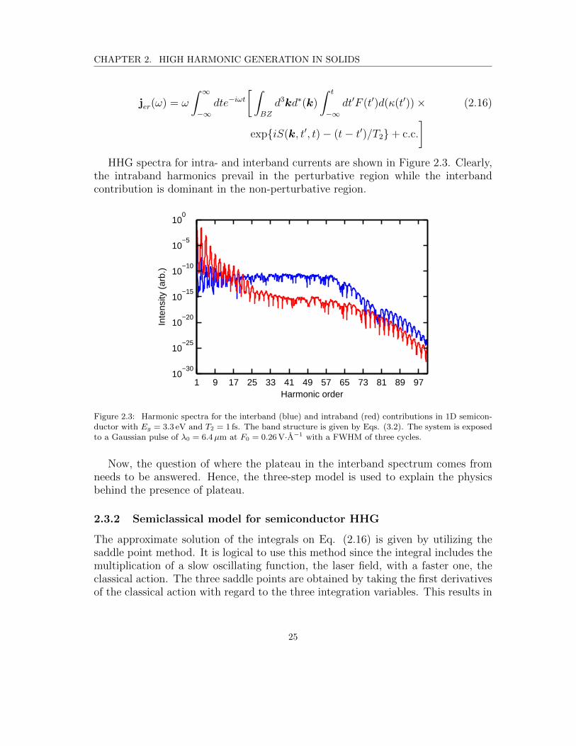
]HHG spectra for intra- and interband currents are shown in Figure 2.3. Clearly,
the intraband harmonics prevail in the perturbative region while the interbandcontribution is dominant in the non-perturbative region.
Harmonic order
Inte
nsity
(ar
b.)
1 9 17 25 33 41 49 57 65 73 81 89 9710
−30
10−25
10−20
10−15
10−10
10−5
100
Figure 2.3: Harmonic spectra for the interband (blue) and intraband (red) contributions in 1D semicon-ductor with Eg = 3.3 eV and T2 = 1 fs. The band structure is given by Eqs. (3.2). The system is exposedto a Gaussian pulse of λ0 = 6.4µm at F0 = 0.26 V·A−1 with a FWHM of three cycles.
Now, the question of where the plateau in the interband spectrum comes fromneeds to be answered. Hence, the three-step model is used to explain the physicsbehind the presence of plateau.
2.3.2 Semiclassical model for semiconductor HHG
The approximate solution of the integrals on Eq. (2.16) is given by utilizing thesaddle point method. It is logical to use this method since the integral includes themultiplication of a slow oscillating function, the laser field, with a faster one, theclassical action. The three saddle points are obtained by taking the first derivativesof the classical action with regard to the three integration variables. This results in
25

CHAPTER 2. HIGH HARMONIC GENERATION IN SOLIDS
∇kS = = ∆xm −∆xm′ = 0 (2.17a)
∂S
∂t′= εg[κ+A(t′)] = 0 (2.17b)
∂S
∂t= εg(k) = ω (2.17c)
where ∆xm =∫ t
t′vm(t′′)dt′′ = xm(t)−∆xm(t′), t′ is the time of electron (hole) birth
from m = c (m = v), and t represents the time of observation. Equation (2.17a)indicates that the electron (hole) that leaves the conduction (valance) band at timet′ returns to the same position after a duration τ = t− t′. Equation (2.17b) statesthat the energy gap at the point κ+A(t′) at the time of birth must be equal to zero;however, the minimum value of εg(k) > 0. Therefore, the parameter κ+A(t′) mustbe complex, so its imaginary part describes tunneling and its real part describespropagation of the pair. The real part then is
k = A(t) +A(t′) = 0. (2.18)
Equation (2.18) implies that an electron and a hole born at t′ at the Γ point areaccelerated by the laser field in the k space. The equation of stationary pointt, Eq.(2.17c), shows that the energy is conserved; the recombination of the pairresults in emitting a photon with energy ω that is equivalent to the energy gap atthe recombination moment.
In general, the physics of the three-step model in solids is very similar to that inatoms, see Eqs.(1.30).
2.3.3 Effect of dephasing on interband vs intraband harmonics
As we stated above, the scattering of electrons with other particles can be rep-resented phenomenologically by dephasing. The coherence between electrons andholes is lost on the scale of T2. If T2 is comparable to the laser pulse duration,then there is enough time to have multiple recollisions. The interference of photonsemitted during different half cycles results in a noisy spectrum. By contrast, ifthe dephasing time is comparable to the laser cycle, recollisions are suppressed andsome of the electrons never return. Short decoherence times affect the interband andintraband contributions to HHG differently. As such, there is the possibility thata small value of T2 may suppress the interband contribution enough, particularlyat longer wavelengths, so that the intraband contribution becomes the dominantcontributor to HHG.
26

CHAPTER 2. HIGH HARMONIC GENERATION IN SOLIDS
This has been examined in Fig. 2.3. The dephasing time T2 is introduced intoour two-band system as was done in Ref. [16]. We solve the two-band equations forour 1D model solid with Eg = 3.3 eV, λ0 = 6.4µm, F0 = 0.26 V·A−1 and T2 = 1 fs.This particular set of parameters represents an extreme case, as the dephasing timeis 1/20th of the optical cycle. Still, Figure 2.3 shows that interband HHG (blue)remains dominant over intraband HHG (red).
27

Chapter 3
HHG in Low-Dimensional SolidState Systems
Here, we theoretically investigate the effect of quantum confinement on high har-monic generation in semiconductor materials. The main idea is the study of strongfield dynamics in nanostructures. The backbone of our investigation is the studyof the effect of varying width of nanostructure on ionization and HHG. The effectsthat quantum confinement has on harmonic generation output are presented in thischapter. The quantum confinement is performed by varying the width of a modelnanostructures. Our analysis reveals a reduction in ionization and a concurrentgrowth in HHG efficiency with increasing confinement. The drop in ionization re-sults from an increase in the bandgap due to stronger confinement. The increase inharmonic efficiency comes as a result of the confinement restricting the spreading ofthe transverse wavepacket. As a result, intense laser driven 1D and 2D nanosystemspresent a potential pathway towards scaling HHG to higher efficiencies and photonenergies.
3.1 Quantum confinement
A confined quantum system is defined as a low-dimensional system where the motionof the carriers (electron and hole) are restricted to a length scale that is comparableto the electron wavelength in one or more directions. Based on the confinementdirection, a quantum confined structure will be classified into three types: quan-tum well (one direction), quantum wire (two directions) and quantum dots (threedirections), where the parentheses represent the number of confinement directions.
A quantum well; for example, can be formed by a thin layer of a narrower-
28

CHAPTER 3. HHG IN LOW-DIMENSIONAL SOLID STATE SYSTEMS
bandgap material that is surrounded by two layers of a wider-bandgap material.The middle layer must be sufficiently thin for quantum properties to be exhibited.For our purpose in this chapter, the width of this layer should be comparable to theunit cell. Because of the difference in Fermi levels, carriers are trapped in the well.Thus, electron and hole are localized in the same region of space, which makes forefficient recombination.
For any of the three structures, the electron momentum is quantized in the con-finement direction. Therefore, the energy along this direction will be limited toa series of discrete values. Along these directions, the continuous energy bandsof bulk material are not valid anymore. In addition, the confinement of particleswithin a small distance leads to an increase in their momentum and energy. Thisband structure directly impacts the electronic and optical properties of the ma-terial which makes these structures efficient in several applications and devices.Nanostructures and its applications have been extensively studied and illustratedin several textbooks, see for example [49].
3.2 Quantum confinement role in enhancing HHG
Quantum diffusion is one of the limitations of HHG, in the gas as well as the con-densed matter phase. It increases the transverse wavepacket width during propa-gation and therewith reduces the recombination probability. Therefore, this resultsin reducing the intensity of the harmonic output. In the atomic case, confiningthe system transversely with a magnetic field can be used to counteract quantumdiffusion and to increase HHG [21].
In solid state systems, quantum diffusion also plays a similar role in the recol-lision process. This impacts the efficiency of interband HHG [15, 16]. Figure 3.1shows a schematic depiction of this process; here the k-space formalism has beentransformed into the Wannier picture where the electron/hole wavefunctions arelocalized in space. When an electron-hole pair is created, they are propagated inthe field. During this propagation, the wave packet spreads leading to a reductionin the recollision cross-section and thus lower harmonic output. In the bulk casewhere there is no confinement, the spreading of the wave packet in space resultsfrom the time-dependent phase contribution from the transverse crystal momentumdistribution; see equation (A.28) for an approximate solution. Here the spreadingof the wave packet will be maximally resulting in a reduction in the recollisioncross-section and thus lowering the harmonic output; see Fig. 3.1(a). By contrast,when the confinement is such that there is only a single transverse state, spreadingof the wave packet will be reduced, or eliminated altogether, resulting in a higher
29

CHAPTER 3. HHG IN LOW-DIMENSIONAL SOLID STATE SYSTEMS
e+e+
e+
e+
e+e+
e+
e+
Birth
Recollision
Birth
Recollision
Unconned system
Maximally conned
system
ElectronHole
Laser
pulse
Harmonic
photon
(a)
(b)
Figure 3.1: Schematic depiction of the effect of quantum confinement on wave packet spreading andinterband harmonics; the black circles represent electrons and the grey circles represent holes. Here the k-space formalism has been transformed into the Wannier picture.(a) In the bulk solid there is no transversalconfinement. When an electron-hole pair is created by the laser field, their wave packets have an initialwidth. As the electron-hole pair is propagated in time (depicted by the black curved arrows) by the field,their wave packets begin to spread. The spreading behavior results from the time-dependent phase fromthe k-space distribution in the transverse direction; see equation (A.28). At the time of recollision, thewave packets will have undergone significant spreading thus reducing their harmonic output. (b) Whenthe system is maximally confined (this would correspond to a one-dimensional system containing only asingle transverse state) the wave packet is unable to spread during propagation in the field. Thus, at thetime of recollision, maximal overlap will occur, resulting in an enhanced harmonic efficiency.
30

CHAPTER 3. HHG IN LOW-DIMENSIONAL SOLID STATE SYSTEMS
ionization probability; see Fig. 3.1(b).
3.3 Methods
3.3.1 Model for confined quantum systems
Our model of the confined systems consists of a single valence band (v) and a singleconduction band (c). It has been noted that multiple bands need to be consideredwhen the system experiences significant Bloch oscillation [50] or when multipleharmonic plateaus are of interest [51]. For the field strengths used here, Blochoscillations are not a significant concern. Further, parameters that are used for ourmodel semiconductor are similar to those used in reference [51] where it was shownthat the first plateau in the harmonic spectrum determined by the two band systemdid not differ significantly to that of the corresponding 51 band system.
The valence and conduction bands in our model can be expressed as Em =∑j Em,j where j = x, y, z and m = c, v. The z direction is chosen to be longitu-
dinal to the laser field. The band gap along each confined transverse direction isdetermined by a periodic potential v(u) (u = x, y). For a single lattice site of widthau and well of depth v0 this is given by,
v(u) =
v0e− u2
σ2u−u2 for 0 ≤ u < σu
v0e− (u−au)2
σ2u−(u−au)2 for au − σu < u ≤ au0 otherwise
(3.1)
where σu = 0.41A. The width along the direction of confinement Lu is determined bychoosing the number of lattice sites. The resulting one-dimensional Hamiltoniansare then diagonalized numerically. When confinement is along both transversedirections we choose equal confinement widths along both directions and denotethis width by L = Lx = Ly. When confinement is along a single direction we willdesignate this as the transverse x direction. In these systems we have L = Lx andwe fix Ly = 50 nm. When L = 50 nm the band structure is nearly identical to thatof the bulk crystal.
We express the band gap for the confined system as εL(k) = εL(n⊥) + ε‖(k‖)where εL(n⊥) = Eg + ε⊥(n⊥, L) and ε⊥ and ε‖ are band gaps in the transverseand longitudinal directions to the field; Eg is the minimum band gap of the bulkcrystal. The transverse confinement causes the band structure to form a discreteset of states. As such, here we define k = (n⊥, k‖) with n⊥ = (nx, ny) being thequantum numbers of the transverse states and k‖ = kz being the longitudinal crystalmomentum. The minimum band gap energy of the confined system is denoted by
31

CHAPTER 3. HHG IN LOW-DIMENSIONAL SOLID STATE SYSTEMS
Table 3.1: Fourier coefficients for the valence and conduction bands of our direct band gap semi-conductor along the z direction [17]. The parameters are for the Γ−M band of ZnO.
Index αj (eV) βj(eV)
0 −2.5242 2.44261 1.9176 −2.21412 0.5440 −0.06533 −0.0326 −0.13064 0.0789 −0.00825 0.0163 −0.0245
EL = εL(1, 1) with nx = ny = 1 being the lowest transverse level. Further, wedenote the bandwidth of our model system as ∆L = max[εL(k)], the maximumdifference between the lowest valence and the highest conduction bands. Finally,when discussing the bulk material along the transverse direction, we will drop theL label and replace n⊥ with k⊥ = (kx, ky) the usual crystal momentum. Note thatthe notation above does not explicitly differentiate between systems confined alonga single direction and those confined along both transverse directions. However, itis implied that when discussing confinement along both transverse directions, theL-label refers to the width of confinement along each of these directions, whereas,when discussing confinement along a single direction, the L-label only refers toconfinement along the x direction.
The longitudinal band gap ε‖ is unaffected by the confinement. This can beexpressed by a Fourier cosine expansion,
Ev,z(kz) =5∑j=0
αj cos(jkzaz) (3.2a)
Ec,z(kz) = Eg +5∑j=0
βj cos(jkzaz) (3.2b)
where ε‖ = Ec,z − Ev,z with Eg being the minimum band gap and az the latticespacing along the z direction. The band coefficients αj and βj are given in Table3.1 and the band structure is shown in Fig. 3.2(a). The dipole parallel to the
longitudinal direction is given by dz(k) =√Ep,z/(2ε2
‖(k)) where Ep,z is the Kane
parameter [52–55]; here we use Ep,z = 0.3 a.u.In our calculations we use Eg = 3.3 eV as the minimum band gap in the bulk
crystal. The lattice periodicity and effective mass are az = 2.8A and mz = 0.098me.
32
CHAPTER 3. HHG IN LOW-DIMENSIONAL SOLID STATE SYSTEMS
Along the transverse directions the wells have a depth of v0 = 13.6 eV and a latticespacing of a = ax,y = 5A. In the bulk limit the effective transverse mass is mx,y =0.053me; Fig. 3.2(b) shows the transverse band gap in this limit. As a result of thequantum confinement, the transverse band structure is arranged into discrete levels;this is demonstrated for L = 2 nm in Fig. 3.2(c). Further, confinement increasesthe band gap as the confinement becomes narrower; this behavior is shown in Fig.3.2(d). Our calculations consider confinement widths in the range from L = 50 nm,where the band structure is very close to that of the bulk, down to L = 1 nm wherethere are only two atomic sites along each confined transverse direction.
(a)
0 0.5 13
5
7
9
11 (b)
0 0.5 13
5
7
9
11
(c)
1 2 3 43
5
7
9
11
(d)
100
101
0
0.5
1
1.5
Figure 3.2: (a) Band gap along the longitudinal and (b) transverse x-direction for the bulk crystal. (c)Band gap along the transverse x-direction for a single confined direction with L = 2 nm. (d) Increase inband gap energy resulting from confinement along a single transverse axis; the dashed lines in (c) and (d)represent the bulk limit.
3.3.2 Ionization dynamics and high harmonic generation
In our analysis of ionization and HHG, we employ the frozen valence band approx-imation [56]. Here it is assumed that the valance band population remains largelyunchanged as a result of the interaction between the solid and laser. With thefrozen valence band approximation, the population transferred from valence to the
33
CHAPTER 3. HHG IN LOW-DIMENSIONAL SOLID STATE SYSTEMS
conduction band can be expressed through,
nc(t) = N∫BZ
∣∣∣∣∫ t
−∞dt′Ω∗(K, t′)eiS(K,t′)
∣∣∣∣2 d3K, (3.3)
where
S(K, t)=
∫ t
−∞εL(K+A(t′)
)dt′. (3.4)
is analogous to the classical action with A(t) being the vector potential. The crystalmomentum k = K+A(t) has been transformed into a frame moving with the vectorpotential; this transformation also results in a transformation of the Brillouin zoneBZ = BZ − A(t). Further, Ω(K, t) = d
(K + A(t)
)· F(t) is the time-dependent
Rabi frequency with d the dipole transition moment. The electric field is deter-mined through F(t) = −dA/dt and N is a constant that ensures normalization ofthe initial valence band population. When performing our calculations, we will beinterested in the final conduction band population versus the width of the confine-ment L; we will denote this quantity as nc(L) = nc(L, t = ∞). The dependenceon L enters through the band structure εL in S(K, t). Finally, our wavefunction isnormalized to unity for each L to ensure an equivalent amount of material is con-sidered when comparing different L’s. What this means is that when confinementis along two transverse directions, four objects of width L/2 are compared witha single object of width L or, in the case of confinement along a single direction,two objects with confinement width L/2 are compared with a single object withconfinement L.
As mentioned above, high harmonic generation in solids can be produced fromtwo currents — an interband current and an intraband current. The interbandterm was demonstrated to be the dominant contributor to above band gap harmon-ics generated in semiconductors exposed to a mid-infrared laser field [10, 16]. Assuch, we will focus on the interband term. It has been verified that the intrabandterm produces harmonics, in the above bandgap range, that are several orders ofmagnitude less intense than those produced by the interband term, thus renderingit negligible for the cases considered in this work. We do note, however, that whendephasing is strong or THz fields are used, the intraband harmonics may become asignificant contributor to HHG [13, 16]. In Sec. 2.3.3, we have demonstrated thateven for a short decoherence time the interband contribution is dominant in theabove bandgap range for the longest wavelength considered in our calculations.
In the frozen valence band approximation [56], the interband current in frequency
34

CHAPTER 3. HHG IN LOW-DIMENSIONAL SOLID STATE SYSTEMS
space can be written as [16],
j(ω) = Nω∫BZ
d3K
∫ ∞−∞dte−iωtd∗
(K + A(t)
)×∫ t
−∞dt′Ω(K, t′)eiS(K,t,t′) + c.c., (3.5)
where S(K, t, t′) =∫ tt′ε(K + A(t′′)
)dt′′. The harmonic spectrum is determined
by taking the magnitude square of equation (3.5). As a measure of the harmonicefficiency, we define the harmonic yield Φ as,
Φ(L) =
∫ EL+∆L
EL
∣∣j(ω)∣∣2dω. (3.6)
Hence, Φ(L) is the total contribution of the allowed above band gap harmonics; seethe inset of Fig. 3.3(d). Finally, we define the yield ratio as Φ(L)/nc(L). This givesa measure of the harmonic yield per ionization event.
The quantum confinement results in two phenomena — an increase of the bandgap and a reduction in the density of transverse states. Both effects will have influ-ence on ionization and HHG. The band gap increase will result in lower ionizationand, consequently, a reduced harmonic output. In contrast, the reduction of thedensity of transverse states will restrict the spreading of the quantum wave packet.This will result in an increase of recollision cross section and therewith an increasein HHG. By varying L alone, these contributions will remain coupled. In order toquantify these two contributions, it is necessary to separate them. This is can beachieved by noting that the ultimate limit of confinement occurs when there is onlya single atom along each confined direction. In the case of the nanowire, the systembecomes an atomic chain and in the case of the quantum sheet, the system becomesa monolayer. By neglecting the transverse coordinates of a 3D bulk material, theband gap of the resulting 1D and 2D mediums remains unchanged. However, thesystem has now gone from no confinement to a maximally confined system. Thus,by comparing the 3D bulk material to its corresponding 1D and 2D limits, we willbe able to isolate the effect resulting from the spreading of the wave packet.
Additionally, we can gain insight by comparing the 3D bulk to its 1D and 2Dlimits through an analytical expression. This can be achieved for both ionizationand HHG, as both can be represented as a product of the confined and non-confinedcontributions. Following the approach of Keldysh/Lewenstein [30,37], saddle pointintegration of equation (3.3) followed by integration over the confined transverse
35

CHAPTER 3. HHG IN LOW-DIMENSIONAL SOLID STATE SYSTEMS
momentum coordinates can be achieved. The conduction band population can be
written as the product nc = n(3−q)Dc nqD⊥ where, n
(3−q)Dc is the contribution from
the longitudinal and unconfined transverse coordinates and nqD⊥ is the confinedtransverse coordinate contribution. The quantity q indicates the number of confinedtransverse coordinates; for the remainder of this work we will use q = 2 to denoteconfinement along both transverse directions and q = 1 for confinement along asingle transverse direction. The contribution coming from the confined transversedirection(s) can then be written as,
nqD⊥ =
(F 2
0
2mzEg
)q/4 q∏j=1
aj
√mj
2π, (3.7)
where j = 1, 2 has been substituted for j = x, y; for a complete derivation ofequation (3.7), see Appendix A. Similarly, by applying saddle point integration toequation (3.5), the 3D current j3D can also be split into an unconfined current term
j(3−q)D and a confined transverse term jqD⊥ where,
|jqD⊥ |2 =
(2mzEgF 2
0
+π2
ω20
)−q/2 q∏j=1
ajmj. (3.8)
In equation (3.8), j and q have the same meaning as in equation (3.7); as withequation (3.7), a derivation of equation (3.8) is provided in Appendix A. Note thatequations (3.7) and (3.8) scale differently with the transverse effective masses mj.Consequently, HHG will be affected more strongly by a change in the effective massof the electron-hole pairs when a different material is used, than will ionization.Finally, for the above expression to be valid, the Keldysh parameter must satisfyγ < 1; all calculations presented here have 0.22 < γ < 0.87.
3.4 Results and Discussion
3.4.1 Ionization and harmonic output
Our confined quantum systems are exposed to an intense laser-field having vec-tor potential A(t) = z(F0/ω0)f(t) cos(ω0t) where ω0 is the driving laser frequencycorresponding to a central wavelength of λ0; the pulse envelope f(t) is Gaussianwith a FWHM of three cycles. The peak field strength is F0 = 0.26 V·A−1; thiscorresponds to a peak field intensity of I0 = 8.8 × 10¹¹ W·cm−2. In Fig. 3.3 thetop four panels (a)-(d) present results for our model system with confinement alongboth transverse directions (q = 2); the bottom four panels (e)-(h) show our resultswhen confinement is only along a single transverse direction (q = 1). Figures 3.3(a)
36

CHAPTER 3. HHG IN LOW-DIMENSIONAL SOLID STATE SYSTEMS
and 3.3(e) show the time-dependence of the population in the conduction band forL = 50 nm (blue) and L = 1 nm (red) with a driving wavelength of λ0 = 6.4µm.The final conduction band population versus confinement width is plotted in Figs.3.3(b) and 3.3(f). For L = 50 nm ionization has reached a plateau and is near tothat of the bulk crystal. As the confinement width is decreased to 1 nm, there isa significant decrease in the final conduction band population. This decline in thefinal population is much more drastic when both transverse directions are confined.In the case where q = 2 (Fig. 3.3(b)) the drop is by several orders of magnitude,whereas, for q = 1 (Fig. 3.3(f)) the drop is just over an order of magnitude.
In both cases, this behaviour can be attributed to the increase in the band gapthat results from the quantum confinement. Since this increase in band gap islarger for when q = 2 — due to the confinement of both transverse directions — ananowire will experience a suppression of ionization that is greater than that of athin slab where confinement is restricted to a single transverse direction. For thefew-cycle pulses used here, optical field ionization is the primary mechanism lead-ing to material damage; other ionization channels, such as collisional ionization, areof sub-ordinate importance. Damage occurs once the conduction band populationreaches the percent level. As a result, from Figs. 3.3(b) and 3.3(e) it follows thatthe damage threshold intensity increases with stronger confinement; that is withdecreasing L.
Further, in accordance with experiments on semiconductors [57], the time dy-namics of the conduction band population for L = 50 nm displays a growth that iswith the laser half-cycle. By contrast, the L = 1 nm results display mainly tran-sient population dynamics with a small carrier density remaining after the pulse,similar to that observed in dielectric experiments [58]. This opens the possibilityto nano-engineer semiconductor materials to be used in PHz optoelectronics whereso far the primary candidates are dielectrics [58–60] or graphene [61].
Figure 3.3(c) shows the harmonic spectra for the q = 2 system with L = 50 nm(blue) and L = 1 nm (red) at λ0 = 6.4µm. The shaded region shows the above bandgap range [EL, EL+∆L] — over which integration in equation (3.6) is performed —for the L = 50 nm system. The spectrum for the 1 nm confinement is shifted due tothe increase in band gap, and thus, the region of integration is shifted accordingly.Figure 3.3(d) displays the harmonic yield determined from equation (3.6) for theq = 2 system. The results for the q = 1 system, corresponding to Figs. 3.3(c) and3.3(d), are presented in Figs. 3.3(g) and 3.3(h). When comparing Figs. 3.3(c) and3.3(g), it can be seen that the increase in harmonic intensity for L = 1 nm is muchmore pronounced when both transverse directions are confined. This behaviour
37

CHAPTER 3. HHG IN LOW-DIMENSIONAL SOLID STATE SYSTEMS
(a)
-5 0 5
Cycle time (T0)
0
1
2
3
Con
d. b
and
popu
latio
n
×10-4
(b)
1 10
L (nm)
10-7
10-6
10-5
10-4
Con
d. b
and
popu
latio
n
(c)
1 21 41 61 81 101
Harmonic order
10-16
10-12
10-8
10-4
Inte
nsity
(ar
b.)
(d)
1 10
L (nm)
10-4
10-3
10-2
Har
mon
ic y
ield
(e)
-5 0 5
Cycle time (T0)
0
1
2
3
Con
d. b
and
popu
latio
n
×10-4
(f)
1 10
L (nm)
10-5
10-4
Con
d. b
and
popu
latio
n
(g)
1 21 41 61 81 101
Harmonic order
10-16
10-12
10-8
10-4
Inte
nsity
(ar
b.) (h)
1 10
L (nm)
10-4
10-3
Har
mon
ic y
ield
Figure 3.3: Panels (a)-(d) present results for our model system with confinement along both transversedirections. (a) Time-dependent conduction band population for L = 50 nm (blue) and L = 1 nm (red) withλ0 = 6.4µm. (b) Conduction band population after the laser pulse has passed versus L for λ0 = 3.2µm(solid) and λ0 = 6.4µm (dash-dot). (c) Harmonic spectra for L = 50 nm (blue) and L = 1 nm (red). Theshaded region shows the above band gap range [EL, EL + ∆L] for the L = 50 nm system. The spectrumfor L = 1 nm is shifted due to the increase in band gap and thus the region of integration is shiftedaccordingly. (d) Harmonic yield versus L for λ0 = 3.2µm (solid) and λ0 = 6.4µm (dash-dot). (e)-(h)Panels (a)-(d) repeated for confinement along a single transverse direction.
38

CHAPTER 3. HHG IN LOW-DIMENSIONAL SOLID STATE SYSTEMS
is reflected in Figs. 3.3(d) and 3.3(h) where the harmonic yield calculated fromequation (3.6) is shown. In both cases there is an increase in harmonic yield fromL = 50 nm to L = 1 nm. However, the increase is greater when confinement is alongboth transverse directions. For L < 3−4 nm the increase in HHG is outweighed bythe drop in ionization so that HHG efficiency declines with decreasing confinementwidth. The harmonic yield is higher for the longer wavelength mainly due to higherionization. For the parameters used here, the wavelength dependence of the HHGprocess, after ionization, has already saturated at 3.2µm (see Fig. 3.5).
L (nm)
Yie
ld r
atio
(a)
100
101
100
101
102
103
104
L (nm)
Yie
ld r
atio
(b)
100
101
100
101
102
Figure 3.4: Yield ratio versus confinement width for λ0 = 3.2µm (solid) and λ0 = 6.4µm (dash-dot)for (a) the confinement along both transverse directions and (b) confinement along a single transversedirection.
The results presented in Fig. 3.3 show an increase in harmonic yield accompaniedby a significant decrease in ionization. As such, it is useful to examine the yield ratioshown in Fig. 3.4. The yield ratio gives the harmonic yield per ionization eventand constitutes a measure of how efficiently population promoted to the conductionband generates above band gap harmonic radiation. Figure 3.4(a) shows the yieldratio for the system with confinement along both transverse directions and Fig.3.4(b) show the corresponding results when confinement is along a single transverse
39

CHAPTER 3. HHG IN LOW-DIMENSIONAL SOLID STATE SYSTEMS
direction. In both cases there is monotonic growth in yield ratio with decreasingconfinement width. This implies that the efficiency, with which electrons promotedto the conduction band create harmonics, is increased as the system becomes moretightly confined. However, when confinement is along both transverse directions,the increase is significantly larger by couple orders of magnitude. Comparing theL = 50 nm to L = 1 nm, there is an increase of nearly three orders of magnitudewhen both directions are confined as compared to about a single order of magnitudewhen confinement is along only one direction. As ionization is the first step in HHG,an increase in harmonic yield efficiency coupled with a decrease in ionization appearscounter-intuitive; in what follows we will explain this observation.
3.4.2 The effect of confinement on diffusion and recollision
In Fig. 3.2 it was shown that quantum confinement causes an increase in the bandgap and a reduction of the density of states along each direction of confinement.Both of these effects have an influence on ionization and high harmonic generation.By varying the width of the confinement, as is done in Figs. 3.3 and 3.4, thesephenomena remain coupled. In order to gauge the importance of each of thesecontributions, it is necessary to separate them. This separation can be achieved bynoting that the absolute limit of confinement occurs when there is only a single atomalong each confined transverse direction. When confinement is along both trans-verse directions this limit is reached for an atomic chain. In the case of confinementalong a single direction this limit is reached for an atomic monolayer. The singleatom wire contains only a single doubly degenerate transverse state and therewithis an idealized one-dimensional system with the same band gap in which confinedtransverse coordinates are neglected. In a similar manner, the monolayer is identicalto an idealized two-dimensional system in which the confined coordinate is ignored.Likewise, by neglecting the confined transverse coordinates of a 3D bulk material,the band gap of the resulting 1D and 2D mediums remain unaltered. However,the quantum confinement has now transformed from no confinement to maximumconfinement. Thus, by comparing a 3D bulk medium with its corresponding 1D and2D limits, the effect resulting solely from quantum confinement can be examined.Comparison of the 1D and 2D limits to the L = 1 nm confinement will allow forthe effect resulting from the change in band gap to be quantified.To compare the 3D bulk to its 1D and 2D limits, we compare the L = 50 nm sys-
tems with q = 2 and q = 1 with their respective 1D or 2D system where the confinedtransverse coordinates have been neglected. These results will be compared againstequations (3.7) and (3.8) given in the previous chapter. Figure 3.5(a) displays theratio of the final conduction band population calculated from equation (3.3) for the1D system to the L = 50 nm system; Fig. 3.5(b) displays the corresponding result
40

CHAPTER 3. HHG IN LOW-DIMENSIONAL SOLID STATE SYSTEMS
λ0 (µm)R
atio
of 1
D to
3D
con
d. b
and
popu
latio
n
(a)
1.6 2.4 3.2 4 4.8 5.6 6.460
80
100
120
λ0 (µm)R
atio
of 2
D to
3D
con
d. b
and
popu
latio
n
(b)
1.6 2.4 3.2 4 4.8 5.6 6.4
9
9.2
9.4
9.6
9.8
10
λ0 (µm)
Rat
io o
f 1D
to 3
D h
arm
onic
yie
ld
(c)
1.6 2.4 3.2 4 4.8 5.6 6.4
105
106
λ0 (µm)
Rat
io o
f 2D
to 3
D h
arm
onic
yie
ld
(d)
1.6 2.4 3.2 4 4.8 5.6 6.4
102
103
Figure 3.5: (a) Ratio of final conduction band population in the 1D system to the L = 50 nm system(circles with solid line) versus λ0; the dashed line gives (n2D
⊥ )−1 predicted by equation (3.7). (b) Ratioof final conduction band population in the 2D system to the L = 50 nm system (circles with solid line)versus λ0; the dashed line gives (n1D
⊥ )−1 predicted by equation (3.7). (c) Ratio of harmonic output fromthe 1D system to the L = 50 nm (solid) and the L = 20 nm (dash-dot) systems versus λ0. The dashed lineshows the prediction for |j2D⊥ |−2 from equation (3.8). (d) Ratio of harmonic output from the 2D systemto the L = 50 nm (solid) and the L = 20 nm (dash-dot) systems versus λ0. The dashed line shows theprediction for |j1D⊥ |−2 from equation (3.8).
41
CHAPTER 3. HHG IN LOW-DIMENSIONAL SOLID STATE SYSTEMS
for the 2D system. Both are compared to (nqD⊥ )−1 from equation (3.7) (dashedline). Equation (3.7) is wavelength independent and the calculated results appearconsistent with this. While the calculated results deviate from the constant valuepredicted by equation (3.7), given its simplicity and the complex nature of ioniza-tion in solids [56], these variations are not unreasonable. Furthermore, the resultsin Figs. 3.5(a) and 3.5(b) indicate that ionization is not strongly affected by theform of the wave packet at birth. Thus, the drop in ionization seen in Figs. 3.3(b)and 3.3(f) results mainly from the increase in the band gap.
Figure 3.5(c) shows the ratio of harmonic output calculated from equation (3.5)of the 1D system to the L = 50 nm (solid) and the L = 20 nm (dash-dot) systemswith confinement along both transverse directions (q = 2); Fig. 3.5(d) shows thecorresponding results for the ratio of harmonic output of the 2D system to theL = 50 nm (solid) and the L = 20 nm (dash-dot) with confinement along a singletransverse direction (q = 1). In both cases, the numerical results are compared
to |jqD⊥ |−2 predicted by equation (3.8) (dashed line). Equation (3.8) predicts thatthe ratio of 1D or 2D output to the 3D harmonic output will increase with wave-length. This rise results from reduced harmonic output of the 3D system due toquantum diffusion which decreases the electron-hole recombination cross section.For the L = 50 nm systems this ratio increases until about 4µm and then begins tosaturate indicating a halt in spreading of the wave packet due to the confinement.Similar behaviour occurs for the L = 20 nm systems but saturation begins at ashorter wavelength. This is consistent with that expected from quantum diffusion.Longer wavelengths experience greater spreading of the transverse wave packet andwill thus be affected more strongly by a narrower confinement. Further, this effectis much stronger for systems with confinement along both transverse directions.This occurs because less diffusion is permitted when both transverse coordinatesare confined as opposed to a single coordinate, as in the 2D system. Finally, ouranalytical model reflects the trend correctly, but the λ2
0 scaling in equation (3.8)understates the power scaling of the wavelength dependence. This indicates thatthe actual ionized transverse wave packet structure might be more complex than theapproximate Gaussian distribution obtained in equations (3.7) and (3.8). Such afact may also explain the unusual elliptic polarization dependence of HHG in solidsobserved by experiment [62].
42

CHAPTER 3. HHG IN LOW-DIMENSIONAL SOLID STATE SYSTEMS
3.5 Summary
In this chapter, we have presented the impacts of quantum confinement along oneand two transverse directions on HHG. The effects of 1D and 2D confinement arequalitatively similar, they are substantially more pronounced in the nanowire. Wehave examined the fact that the quantum confinement causes a widening of the bandgap and a reduction of the density of states. These two results have their directimpact on the ionization and harmonic yield. The increase of the band gap leads toa decrease of the final conduction band population. That results in a suppressionof the ionization which presents an advantage since it leads to raising the damagethreshold intensity of the material when the laser source is a few-cycle pulse. Thefew-cycle pulse is essential here to guarantee there are no other ionization channelsexcept the optical field ionization. On the other hand, the reduction of the densityof transverse states reduces quantum diffusion. This results in an increase of therecollision cross-section; therefore, an increase in the HHG efficiency.
Our results suggest that nano-engineering might present a way to surmount someof the restrictions placed on generating high order harmonics from semiconductormaterials. Further, our findings offer a potential explanation for the increase inharmonic efficiency found in recent experiments, where bulk HHG was comparedto atomically thin monolayers of crystalline MoS2 [18].
Finally, our analysis is performed within the single electron approximation. Inlow dimensional materials, correlation effects can become significant; these effectsare neglected in our investigation.
Future research can be concentrated on using stacked lower-dimensional systemsto enhance the harmonic output. The use of these systems is a potential way tosuppress the limitation that comes from absorption. In such systems, propagationoccurs in the gaps between the material layers, where no reabsorption exists.
43
Chapter 4
Impurity Tomography
In 2004, Itatani et al. [25] proposed an experimental method to image the highestoccupied electronic orbital of nitrogen. Their strategy is based on what has beenintroduced in Sec. (1.4). Other experiments demonstrated the reconstruction oforbitals for a more complex molecule such as carbon dioxide [24]. Here we translatethis method from the gas to the solid state phase by using impurities. The problemof impurities in semiconductors has been mapped to the hydrogen-like atom bythe effective mass theorem [63–65]; as compared to the hydrogen atom, electronmass and dielectric constant are different. Due to this similarity, we theoreticallyreconstruct the impurity wavefunction by the same method that has been introducedin imaging of molecular orbitals.
In this chapter, the three-step model for high harmonic generation from shallowdonor impurity in solid is developed. Then, we use the model to investigate thetomographic reconstruction of the impurity ground state wavefunction from har-monic spectra. The impurity dipole moment is found to be the dominant factor indetermining the magnitude of the harmonic signal as a function of harmonic order;ionization and propagation which have to be factored out in molecular tomographyplay a lesser role here. This indicates a substantial facilitation due to the potentialfor direct reconstruction of the impurity ground state from the harmonic spectrum.
4.1 HHG in doped semiconductors
In the following HHG from impurities driven by long wavelength, laser fields isinvestigated. Quantum equations of motion and a three-step model for this processare developed. Figure 4.1 depicts a schematic representation for HHG from shallowimpurities in one dimension. In Fig. 4.1(a) we have the periodic potential of the
44

CHAPTER 4. IMPURITY TOMOGRAPHY
Figure 4.1: (a) Periodic potential of the unperturbed bulk solid (blue) plus the impurity potential (red);the shalloe impurity ground state that extends over many lattice cites is represented by the shadedcurve. (b) Space representation of the three-step model for HHG from an impurity. (c) Reciprocal spacerepresentation of the three-step model for HHG from an impurity.
45

CHAPTER 4. IMPURITY TOMOGRAPHY
unperturbed solid (blue) plus a Coulomb potential from an impurity (red). Theshaded curve represents the ground state of the shallow impurity; this ground stateextends over many lattice cites. The semiclassical description of HHG is given bythe three-step model. First, a free electron/hole is created in the conduction/valenceband by tunnel ionization of a donor/acceptor impurity. Second, the electron/holeis accelerated by the laser field. In a third step a harmonic photon is emitted uponrecollision and recombination with the parent impurity. The three-step model isshown in the real and reciprocal space in Figs. 4.1(b) and 4.1(c), respectively, forthe system interacting with a strong laser field.
Besides differences in the continuum evolution due to the non-parabolic natureof bands, the process is found to be identical to HHG in gases. As a consequence,many processes can be adapted from the gas to the condensed matter phase. Thisopens a new research direction for atomic and molecular strong field processes.
4.1.1 Quantum mechanical model
Our one-body analysis builds on, and extends, the theoretical work by Adams [63]and by Luttinger and Kohn [64,65]. We use the following model: an impurity withpotential U(x) is imbedded in a solid and is coupled to a laser field F(t) via thedipole coupling term x · F(t). The resulting time-dependent Schrodinger equationis given by
i∂tΨ(x, t) = (Hi − x · F(t)) Ψ(x, t), (4.1)
where Hi = H0 + U(x) and H0 = 12p2 + v(x) refers to the Hamiltonian of the solid
without impurity with v(x) being the periodic lattice potential. The eigenvalueequation of the field free Hamiltonian Hi is given by
Hiφ(x, t) = εφ(x, t). (4.2)
In the absence of the impurity the eigenfunctions Φm,k fulfil H0Φm,k = Em(k)Φm,k
with m the band index and Em(k) the band eigenenergies. Further, the eigenfunc-tions are given by,
Φm,k(x) =1√Vum,k(x)eik·x, (4.3)
where um,k is the Bloch function that is periodic with the lattice and V the volumeof the solid. The unit cell is defined by basis vectors al (l = 1, 2, 3) and volumeυ; Rn =
∑l nlal is a lattice vector that connects two identical sites in the lattice.
The crystal momentum k extends over the first Brillouin zone (BZ) defined as the
46

CHAPTER 4. IMPURITY TOMOGRAPHY
Wigner-Seitz cell of the reciprocal lattice whose primitive vectors bl are determinedthrough bl · aj = 2πδlj; we denote the magnitude of the reciprocal lattice vector blas bl = |bl| . The vectors of the reciprocal lattice are given by Kn =
∑l nlbl. The
eigenfunctions are orthonormalized according to,∫V
Φ∗m′,k′Φm,kdx = δmm′δ(k− k′). (4.4)
By defining V = Nυ with N the number of atomic unit cells, we obtain from theorthonormality relation
∫v|um,k|2dx = υ.
Shallow donor (acceptor) impurities split into an electron (hole) and a positively(negatively) charged residual ion; the electron (hole) moves in the lowest conduction(highest valence) band and has bound states in the field of the residual ion withenergies closely below (above) the bottom (top) of the conduction (valence) band.As a result, we drop the band index m and confine our treatment to a single bandwith eigenfunctions Φk which fulfil H0Φk = E(k)Φk with E(k) the band eigenener-gies. Further, we consider a single impurity level (the impurity ground state) witheigenenergy ε0 and eigenfunction φ0; here Eq. (4.2) reads,
Hiφ0(x) = ε0φ0(x). (4.5)
As this is a first conceptual study we have limited ourselves to only the most fun-damental process and confined our system to the ground state only. Additionalcomplexity can be added to the model by including excited states of the impuritypotential.
4.1.2 Derivation of the ground state for a shallow impurity
Equation (4.5) is solved by expanding the eigenstate φ0 in terms of Bloch states,
φ0(x) =
∫BZ
b0(k)Φk(x)dk. (4.6)
Inserting Eq. (4.6) into Eq. (4.5), multiplying the result by Φ∗k′(x) and integratingover the spatial coordinate yields,(
E(k)− ε0
)b0(k) +
∫BZ
U(k,k′)b0(k′)dk′ = 0 (4.7)
with
U(k,k′) =
∫V
u∗k(x)uk′(x)U(x)ei(k′−k)·xdx, (4.8)
47

CHAPTER 4. IMPURITY TOMOGRAPHY
where integration if performed over the crystal volume V . By noting that uk isperiodic with the unit cell, the Bloch functions in Eq. (4.8) can be expanded in aFourier series,
u∗k(x)uk′(x) =1√υ
∑n
M(n)k,k′e
−iKn·x (4.9)
with
M(n)k,k′ =
1√υ
∫υ
u∗k(x)uk′(x)eiKn·xdx. (4.10)
As a result, we obtain for the Coulomb matrix element
U(k,k′) =∑n
M(n)k,k′
∫υ
U(x)ei(k′−k−Kn)·xdx (4.11)
By inserting the series expansion (4.9) into the orthonormality relation for the Blocheigenfunction (4.4) we obtain the relation
1√υ
∫υ
M(0)k,k′e
i(k−k′)·xdx = δ(k− k′). (4.12)
Note that expansion terms with n 6= 0 result in δ(k − k′ −Kn) = 0, as k,k′ arefrom the first BZ. Equation (4.12) yields
M(0)k,k′ =
√υ
(2π)3. (4.13)
For a soft potential whose main components correspond to wavelengths that aremuch smaller than the lattice spacing, |k − k′| bl the lowest order Fourier termdominates and we obtain [63,64]
U(k− k′) ≈√υ
(2π)3
∫υ
U(x)ei(k′−k)·xdx. (4.14)
where we have written U(k,k′) as U(k − k′) to indicate that the argument in Uof our approximate expression above depends only on the difference k − k′. Notethat close to the Coulomb singularity this assumption is violated and higher orderFourier terms need to be included. Inserting Eq. (4.14) in Eq. (4.7) yields
(E(k)− ε0) b0(k) +
∫BZ
U(k− k′)b0(k′)dk′ = 0. (4.15)
48
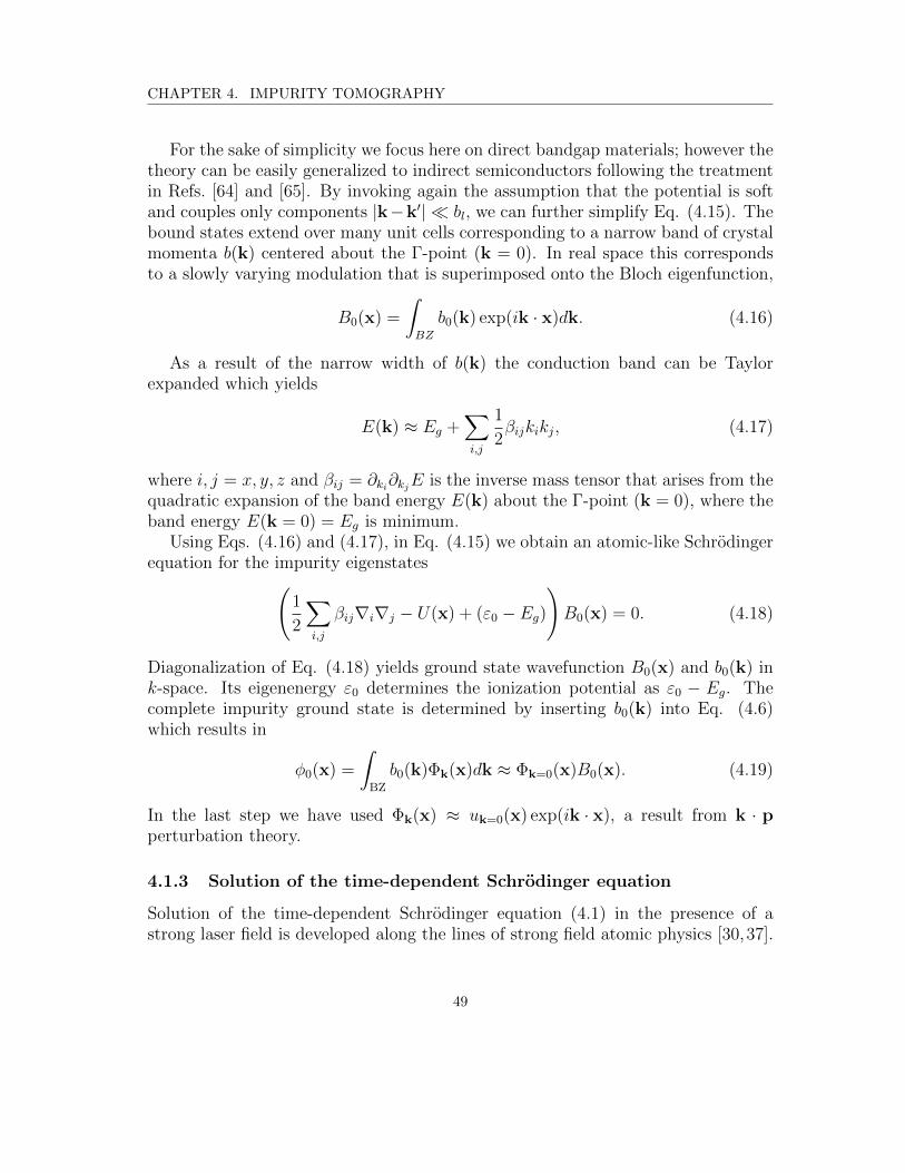
CHAPTER 4. IMPURITY TOMOGRAPHY
For the sake of simplicity we focus here on direct bandgap materials; however thetheory can be easily generalized to indirect semiconductors following the treatmentin Refs. [64] and [65]. By invoking again the assumption that the potential is softand couples only components |k−k′| bl, we can further simplify Eq. (4.15). Thebound states extend over many unit cells corresponding to a narrow band of crystalmomenta b(k) centered about the Γ-point (k = 0). In real space this correspondsto a slowly varying modulation that is superimposed onto the Bloch eigenfunction,
B0(x) =
∫BZ
b0(k) exp(ik · x)dk. (4.16)
As a result of the narrow width of b(k) the conduction band can be Taylorexpanded which yields
E(k) ≈ Eg +∑i,j
1
2βijkikj, (4.17)
where i, j = x, y, z and βij = ∂ki∂kjE is the inverse mass tensor that arises from thequadratic expansion of the band energy E(k) about the Γ-point (k = 0), where theband energy E(k = 0) = Eg is minimum.
Using Eqs. (4.16) and (4.17), in Eq. (4.15) we obtain an atomic-like Schrodingerequation for the impurity eigenstates(
1
2
∑i,j
βij∇i∇j − U(x) + (ε0 − Eg)
)B0(x) = 0. (4.18)
Diagonalization of Eq. (4.18) yields ground state wavefunction B0(x) and b0(k) ink-space. Its eigenenergy ε0 determines the ionization potential as ε0 − Eg. Thecomplete impurity ground state is determined by inserting b0(k) into Eq. (4.6)which results in
φ0(x) =
∫BZ
b0(k)Φk(x)dk ≈ Φk=0(x)B0(x). (4.19)
In the last step we have used Φk(x) ≈ uk=0(x) exp(ik · x), a result from k · pperturbation theory.
4.1.3 Solution of the time-dependent Schrodinger equation
Solution of the time-dependent Schrodinger equation (4.1) in the presence of astrong laser field is developed along the lines of strong field atomic physics [30,37].
49

CHAPTER 4. IMPURITY TOMOGRAPHY
The wavefunction is split into a bound state part and a band contribution, by usingthe Ansatz
Ψ(x, t) = φ0(x) +
∫BZ
a(k, t)Φk(x)dk. (4.20)
where the integral runs over the first BZ. We assume, in the spirit of the strong fieldapproximation [30], that field induced ionization is weak enough so that the groundstate population remains unaffected. This amounts to neglecting the dynamic Starkshift of the impurity ground state.
Inserting Eq. (4.20) into Eq. (4.1) and multiplying the resulting equation withthe functional 〈Φk′(x)| we obtain
id
dta(k, t) = (E(k)− ε0 + iF(t) · ∇k) a(k, t)
+
∫BZ
U(k− k′)a(k′, t)dk′ + id0(k) · F(t), (4.21)
where the transition dipole moment between impurity ground state and conductionband is,
d0(k) =
∫V
Φ∗k′(x)xφ0(x)dx. (4.22)
Equation (4.21) is similar to the equation of atomic strong-field physics [30]. Aroundthe Γ-point, where the effective mass approximation is valid, Eq. (4.21) becomesidentical with the equation for atomic gases. We note, however, that in Eq. (4.21)the full band is used and not the effective mass approximated band in Eq. (4.17).
Here we have again employed the assumptions used for the derivation of theimpurity potential matrix element (4.14) where a soft impurity potential is assumedfor which large momentum scattering |k| > |bl| is negligible. In terms of dynamicalprocesses, these assumptions amount to neglecting large angle scattering events ofthe order of or larger than the inverse lattice vectors, which occur when a slowelectron comes close to the Coulomb singularity and undergoes scattering. Furtherthe resulting intraband dipole matrix element is only well defined when writtenas [16] ∫
V
Φ∗k′(x)xΦk(x)dx = −i∇k + dc(k), (4.23)
where
dc = −i∫V
Φk′(x)∇kΦk(x)dx. (4.24)
50

CHAPTER 4. IMPURITY TOMOGRAPHY
We assume here inversion symmetric materials for which dc = 0. As long as impurityground state and conduction band wavefunction vary slowly compared to the Blochfunctions, the dipole moment between impurity ground state and conduction bandis given by,
d0(k) ≈ 1
(2π)3
∫V
xB0(x)e−ik·xdx. (4.25)
Here we have applied again Eq. (4.13) to approximately eliminate the product ofBloch functions. We find that the dipole moment is proportional to the Fouriertransform of the atom-like part of the impurity ground state, just as in the atomicstrong field model. Finally, agreement with atomic strong field physics becomescomplete, when the quadratic mass approximation is applied to Eq. (4.21) [30,37].
In the strong field limit, the Coulomb potential in Eq. (4.21) is neglected. Forimpurities, additional justification comes from the fact that photoionization crosssections are well described by replacing the Coulomb with delta-function potentials[66]. Integration of the resulting Eq. (4.21) and inserting the result into the secondterm of Eq. (4.6) yields the time dependent evolution of the electron wavefunctionin the conduction band as
a(k, t)=
∫ t
−∞dt′d0(κt′)·F(t′)e
∫ t′−∞i(ε0−E(κt′′ )+
iT2
)dt′′
(4.26)
where κt′ = k − A(t) + A(t′) with vector potential determined by F = −dA/dt;further, a phenomenological dephasing time T2 has been added.
Finally, high harmonic generation is determined by the current
j(t) =d
dt
∫V
x|Ψ(x, t)|2dx
=d
dt
∫BZ
a(k, t)d∗0(k)dk +
∫BZ
(a∗(k′, t)a(k, t)
× 1
i
∫V
Φ∗k′(x)∇Φk(x)dx)dk′dk + c.c. (4.27)
The second term in Eq. (4.27), corresponding to the intraband current, comes as aresult of changing the Schrodinger picture to the Heisenberg picture, using dx/dt =p and then converting back to the Schrodinger picture. Further simplification canbe made using the relation,
1
i
∫V
Φ∗k′(x)∇Φk(x)dx = ∇kE(k)δ(k− k′) (4.28)
51

CHAPTER 4. IMPURITY TOMOGRAPHY
with v(k) = ∇kE(k) the band velocity. We then obtain
j(t) = ji(t) + jra(t), (4.29)
where
ji(t) =d
dt
∫BZ
a(k, t)d∗0(k)dk + c.c. (4.30)
is the current due to the polarization buildup between band electron and impurity,and
jra(t) =
∫BZ
|a(k, t)|2v(k)dk + c.c. (4.31)
is the intraband current arising from the laser driven motion of the electron in theband; this contribution comes from the non-parabolicity of the band and is notpresent in HHG from atomic gases.
4.1.4 Semicalssical model for impurity high-harmonic generation
The high harmonic electric fields are determined by the polarization buildup be-tween band and impurity ground state resulting in a current
ji(ω) = iω
∫BZ
dk d∗0(k)
∫ ∞−∞dte−iωt
∫ t
−∞dt′d0(κt′)·F(t′)
× e(iS(k,t′,t)− 1
T2(t−t′)
)dt′′
+ c.c. (4.32)
where S(k, t′, t) =∫ tt′
(ε0 − E(κt′′)
)dt′′.
The three integrals in Eq. (4.32) can be solved analytically by the saddle pointmethod [30]. The saddle point equations are determined by,
∇kS =
∫ t
t′v(κt′′)dt
′′ = x(t)− x(t′) = 0 (4.33a)
dS
dt′= E(k−A(t) + A(t′))− ε0 = 0 (4.33b)
dS
dt= E(k)− ε0 = ω. (4.33c)
In Eq. (4.33a), the band velocity is given by v(k) = ∇kE. This equation statesthat HHG can take place only when the electron, born at time t′ into the band,returns to the parent impurity at t. Equation (4.33b) states that electrons areborn with zero momentum at time t′, k = A(t = t′) −A(t′) = 0. At the time of
52

CHAPTER 4. IMPURITY TOMOGRAPHY
recombination t the electron crystal momentum is given by k(t′, t) = A(t)−A(t′).The finite impurity gap energy results in a complex birth time, which is responsiblefor tunnel ionization. Finally, Eq. (4.33c) represents conservation of energy — theelectron recombines to the ground state and emits a photon ω with energy equalE(k(t′, t)) − ε0. Again, at moderate laser intensities, for which the effective massapproximation applies, the saddle point equations for atom and impurity becomeidentical.
After saddle point integration we obtain for the harmonic intensity
∣∣ji(ω)∣∣2 =
∣∣∣∣∣∑t′
√w(t′)d∗0(k)α(t′, t)e
∫ tt′
(iS− 1
T2
)dt′′
∣∣∣∣∣2
, (4.34)
where S = ε0 + ω − E(k(t′′, t)
), w(t′) is the ionization rate and t′(t(ω)) and t(ω)
are birth and recombination times resulting in the generation of a harmonic withfrequency ω. For an isotropic lattice the ionization rate is determined by the ADKtunnel ionization rate of atoms [67] with the electron mass replaced by the effectivemass. Further, the dipole moment represents the recombination amplitude; theremaining term α in the pre-exponential is the propagation amplitude accounting forquantum diffusion and dephasing; this depends on the band specifics. For isotropicmaterials in the effective mass m approximation α ∝ m exp(−(t− t′)/T2)(t−t′)−3/2.The main difference between HHG from impurities and atoms arises from the finite,non-parabolic, anisotropic nature of bands.
4.2 Numerical details
For the analysis of HHG tomography of impurities we use a 1D model system fora direct band gap semiconductor. The periodic lattice potential is composed oflattice cells of width a = 9.45 a.u. = 5 A and well depth v0 = 0.55 a.u. = 15 eV. Thelattice cells are separated by a mollifier function, see Section.(3.3.1); the lattice cellcentered at x = 0 is given by,
v(x) =
v0e− (x+a/2)2
σ2−(x+a/2)2 − v0 for − a2≤ x < −a
2+ σ
v0e− (x−a/2)2
σ2−(x−a/2)2 − v0 for a2− σ < x ≤ a
2
−v0 otherwise
(4.35)
where σ represents the extension of the mollifier. Each cell is represented on aspace grid of 40 points giving a grid spacing of ∆x = 0.236. We use 400 cells to theleft and right of the central cell for a total of 801 cells. The Coulomb potential is
53

CHAPTER 4. IMPURITY TOMOGRAPHY
centered over the central cell and is given by,
U(x) =−1
ε√x2 + s2
, (4.36)
where s is the softening parameter and ε is the dielectric constant. For our modelwe use s = 25 a.u. and ε = 5 a.u.
The Hamiltonian is diagonalized using periodic boundary conditions in both thepresence and absence of the Coulomb potential. In the absence of the Coulombpotential we obtain the Bloch functions Φk(x); the energy gap between the highestvalence band and lowest conduction band at the Γ−point is approximately 4 eV.When the Coulomb potential is present we obtain the impurity ground state; forthis system the impurity ground state lies at an energy of 106.4 meV below theΓ−point of the conduction band. Figure 4.2(a) shows the calculated conductionband versus the crystal momentum k. In Fig. 4.2(b) the dipole moment calculatedfrom Eq. (4.25) is shown.
The system is irradiated by a laser field with vector potential A(t) = −(F0/ω0)f(t) sin(ω0t) with peak field strength F0 and center frequency ω0. The peak fieldstrength is F0 = 1 × 10⁻⁴a.u. which corresponds to a peak intensity of I0 =3.5×10⁸ W/cm2 in the material. For the center frequency we use ω0 = 9.1×10⁻⁴ a.u.;this corresponds to a wavelength of λ0 = 50µm. The pulse has a Gaussian envelopef(t) with a FWHM of 12T0; here T0 = 2π/ω0 = 166 fs. The time dynamics of thesystem are determined from Eq. (4.26) with T2 = 50 fs. The dephasing time T2 ischosen such that it is similar to dephasing times in semiconductors [68–70].
The parameters of our laser pulse and model system result in a result in aminimum n = 5 photon transition from impurity ground state to the conductionband using a pulse with an intensity of the order of 108 W/cm2. For comparison ZnOhas a Γ−point energy of 3.3 eV between the highest valence and lowest conductionband; doping with impurities such as H, Ga, Al and In leads to impurity donorstates in the range 46− 73 meV [71]. For a similar n = 5 photon transition, such asystem would require a laser pulse with central wavelength ∼ 100µm with intensity∼ 100 MW/cm2 which is achievable [72]. By contrast ZnSe has a bandgap of 2.8 eVwith a donor level 1.2 eV below the bottom of the conduction band when dopedwith V [73]. Thus, the parameters chosen here give a reasonable approximation toa semiconductor with shallow donor impurity levels.
54
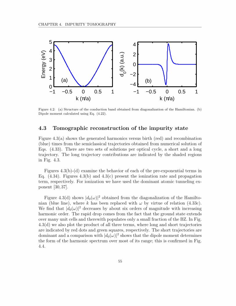
CHAPTER 4. IMPURITY TOMOGRAPHY
k (π/a)
Ene
rgy
(eV
)
(a)
−1 −0.5 0 0.5 10
1
2
3
4
5
k (π/a)
d 0(k)
(a.u
.)
(b)
−1 −0.5 0 0.5 1−4
−2
0
2
4
Figure 4.2: (a) Structure of the conduction band obtained from diagonalization of the Hamiltonian. (b)Dipole moment calculated using Eq. (4.22).
4.3 Tomographic reconstruction of the impurity state
Figure 4.3(a) shows the generated harmonics versus birth (red) and recombination(blue) times from the semiclassical trajectories obtained from numerical solution ofEqs. (4.33). There are two sets of solutions per optical cycle, a short and a longtrajectory. The long trajectory contributions are indicated by the shaded regionsin Fig. 4.3.
Figures 4.3(b)-(d) examine the behavior of each of the pre-exponential terms inEq. (4.34). Figures 4.3(b) and 4.3(c) present the ionization rate and propagationterm, respectively. For ionization we have used the dominant atomic tunneling ex-ponent [30,37].
Figure 4.3(d) shows |d0(ω)|2 obtained from the diagonalization of the Hamilto-nian (blue line), where k has been replaced with ω by virtue of relation (4.33c).We find that |d0(ω)|2 decreases by about six orders of magnitude with increasingharmonic order. The rapid drop comes from the fact that the ground state extendsover many unit cells and therewith populates only a small fraction of the BZ. In Fig.4.3(d) we also plot the product of all three terms, where long and short trajectoriesare indicated by red dots and green squares, respectively. The short trajectories aredominant and a comparison with |d0(ω)|2 shows that the dipole moment determinesthe form of the harmonic spectrum over most of its range; this is confirmed in Fig.4.4.
55

CHAPTER 4. IMPURITY TOMOGRAPHY
Harmonic order
Tim
e (T
0)
(a)
Short
Long
Birth
Recombination
0 20 40 60 800
0.2
0.4
0.6
0.8
1
Harmonic orderIo
niza
tion
rate
(b)
0 20 40 60 8010
−2
10−1
Harmonic order
Pro
paga
tion
(c)
0 20 40 60 80
10−6
10−5
10−4
10−3
10−2
10−1
Harmonic order
|d0(ω
)|2 (
a.u.
)
(d)
0 20 40 60 80
10−6
10−4
10−2
100
102
Figure 4.3: (a) Birth time t′ (red) and return times t (blue) from the semiclassical trajectories versusharmonic order. (b) Ionization rate w ∝ exp
(− 2
3
√m(2(Eg − ε0))3/2/F (t′)
)versus harmonic order. (c)
Propagation effects α2 ∝ exp(− 2(t − t′)/T2
)/(t − t′) versus harmonic order. (d) Magnitude squared
of the dipole moment as a function of harmonic order (blue); the product of the three pre-exponentialterms in Eq. (4.34) represented by blue lines in (b)-(d) is plotted for the short (red dots) and long (greensquares) trajectory branches; the magnitude is adapted to match the dipole moment. In (a) - (c) theshaded regions indicate the contributions from long trajectories.
56
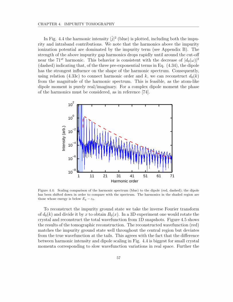
CHAPTER 4. IMPURITY TOMOGRAPHY
In Fig. 4.4 the harmonic intensity |j|2 (blue) is plotted, including both the impu-rity and intraband contributions. We note that the harmonics above the impurityionization potential are dominated by the impurity term (see Appendix B). Thestrength of the above impurity gap harmonics drops rapidly until around the cut-offnear the 71st harmonic. This behavior is consistent with the decrease of |d0(ω)|2(dashed) indicating that, of the three pre-exponential terms in Eq. (4.34), the dipolehas the strongest influence on the shape of the harmonic spectrum. Consequently,using relation (4.33c) to connect harmonic order and k, we can reconstruct d0(k)from the magnitude of the harmonic spectrum. This is feasible, as the atom-likedipole moment is purely real/imaginary. For a complex dipole moment the phaseof the harmonics must be considered, as in reference [74].
Harmonic order
Inte
nsity
(ar
b.)
1 11 21 31 41 51 61 7110
−8
10−6
10−4
10−2
100
102
Figure 4.4: Scaling comparison of the harmonic spectrum (blue) to the dipole (red, dashed); the dipolehas been shifted down in order to compare with the spectrum. The harmonics in the shaded region arethose whose energy is below Eg − ε0.
To reconstruct the impurity ground state we take the inverse Fourier transformof d0(k) and divide it by x to obtain B0(x). In a 3D experiment one would rotate thecrystal and reconstruct the total wavefunction from 1D snapshots. Figure 4.5 showsthe results of the tomographic reconstruction. The reconstructed wavefunction (red)matches the impurity ground state well throughout the central region but deviatesfrom the true wavefunction at the tails. This agrees with the fact that the differencebetween harmonic intensity and dipole scaling in Fig. 4.4 is biggest for small crystalmomenta corresponding to slow wavefunction variations in real space. Further the
57

CHAPTER 4. IMPURITY TOMOGRAPHY
small oscillations in the harmonic spectrum in Fig. 4.4 do not appear to causea substantial error in the reconstruction; they result from interference betweenharmonics generated in positive and negative half-cycles as a consequence of thephase term in Eq. (4.34).
x (a.u.)
|B0(x
)|
11 unit cells
−200 −150 −100 −50 0 50 100 150 2000
0.2
0.4
0.6
0.8
1
Figure 4.5: Comparison between the impurity ground state (blue, shaded) and the reconstructed groundstate (red). The region between the vertical dashed lines represents 11 unit cells.
4.4 Dimensionality considerations for tomographic recon-struction
In our semiclassical model the ionization rate w(t′) and the propagation term thataccounts for quantum spreading and dephasing α(t′, t), are given by,
w(t′) ∝ e−23
√m(2E0)3/2/F (t′) (4.37a)
α(t′, t)2 ∝ e−2(t−t′)/T2
(t− t′)D(4.37b)
where E0 = Eg− ε0 is the impurity ionization potential, D ∈ 1, 2, 3 is the dimen-sion and t′ and t are the birth and recombination times, respectively. The effectivemass along the direction longitudinal to the laser polarization is given by m. InEq. (4.37b) the term (t − t′)−D accounts for the quantum spreading and the terme−2(t−t′)/T2 accounts for the effect of dephasing. Both terms have the strongest effecton the long trajectories as (t− t′) will be greatest for this trajectory branch.
58

CHAPTER 4. IMPURITY TOMOGRAPHY
Harmonic order
|d0(ω
)|2 (
a.u.
)
(a)
0 20 40 60 80
10−6
10−4
10−2
100
102
Harmonic order
|d0(ω
)|2 (
a.u.
)
(b)
0 20 40 60 80
10−6
10−4
10−2
100
102
Figure 4.6: Magnitude squared of the dipole moment as a function of harmonic order (blue); the product ofthe three pre-exponential terms in Eq. (2.51) of the main manuscript is plotted for the short (red dots) andlong (green squares) trajectory branches for (a) the one-dimensional system and (b) a three-dimensionalsystem. The magnitude of the semiclassical curves is adapted to match the dipole moment.
The exponential scaling of the ionization rate only depends on the longitudinalcomponents of the system along the direction of laser polarization; the transversecomponents only appear in the pre-exponential factor. As such, the dimensionalityof the system is not expected to have a significant effect on the form of the ionizationrate. Contrastingly, the quantum diffusion contribution (t−t′)−D to the propagationterm in Eq. (4.37b) will exhibit greater spreading for a three-dimensional systemas opposed to a one-dimensional system.
Figure 4.6 shows the effect the dimension will have on the product w(t′) |d0(k(t′,t))|2α(t′, t)2 in Eq. (4.34). Figure 4.6(a) shows this product for the one-dimensionalsystem; this is a reproduction of Fig. 4.3(d). Figure 4.6(b) shows the productwith D = 3. The three-dimensional plot displays two main difference from theone-dimensional case. First, the separation between the long and short trajectorybranches is greater in three dimensions than in one dimension. This occurs becausespreading can occur in all three directions in the three-dimensional case. Secondly,because the spreading term is more pronounced in three-dimensions, the semiclas-sical curve deviates more from the behaviour of the dipole. This suggests that, forthree-dimensional systems, it may be necessary to account for quantum diffusionbefore reconstructing the wavefunction. Accounting for quantum diffusion shouldbe achievable in a straightforward manner using Eq. (4.34). For each birth andrecombination time pair, α(t′, t) can be calculated. This (t′, t) pair corresponds toa particular harmonic and thus, we have the mapping α(t′, t) → α(ω). The α(ω)term can then be factored out of the harmonic spectrum, removing the effect of
59
CHAPTER 4. IMPURITY TOMOGRAPHY
quantum diffusion for harmonic with frequency ω.
4.5 Summary
Because of the similarity between an atomic system and a doped semiconductorwith donor impurities, one can apply the physics of HHG tomography in atoms andmolecules on the doped semiconductor to image the wave function of the impurityground state.
We calculate the harmonic spectrum by factorizing its three contributions: ion-ization, propagation, and recombination dipole. Our 1D harmonic spectrum cal-culation depicts that the dipole moment has the most significant influence on theharmonic spectrum shape. Prominently, there is a small dissimilarity between thespectrum and the dipole moment that gets greater for small crystal momenta.
Following the same procedure as in the atomic strong field, the inverse of Fouriertransform of the dipole moment between the impurity state and conduction banddivided by x gives the image of the impurity wave function. The reconstructedwave function matches the impurity wave function at the center, but it deviatesat the ends. This deviation harmonizes with the difference between the spectrumand the dipole scaling. For 3D calculation, one must consider quantum diffusionbefore reconstructing the wavefunction. That is because the spreading occurs inthree directions, unlike our calculations where it plays an insignificant role.
A more sophisticated reconstruction scheme could also remove the effects stem-ming from ionization. As a result of the complexity in calculating ionization ratesin solids [56, 75–78], the ionization rate could be measured by transient absorptionspectroscopy [57] and then factored out of the harmonic spectrum in a similar man-ner to that described for removing the effects of quantum diffusion. Furthermore,the dipole moment extracted from Eq. (4.34) or from numerical analysis can beimproved on by using optimization techniques, similar to the one used recently forall optical band gap measurements [79]. Finally, for non-centrosymmetric materialsthe phase of the dipole is also important [80], facilitating the need for the phase ofthe harmonics to be measured for proper reconstruction.
60
Conclusions
High harmonic generation from low-dimension and doped semiconductors has beeninvestigated in this dissertation. The effect that quantum confinement along oneor two transverse directions has on high harmonic generation in semiconductor ma-terials has been theoretically investigated. By reducing the density of states alongthe confined transverse direction, quantum spreading is reduced and the probabilityof recollision is increased. Further, the band gap is widened resulting in a higherdamage threshold of the material. While the population transferred to the conduc-tion band decreases monotonically with increasing confinement, the efficiency withwhich this population creates above band gap harmonics is increased. Further, thiseffect is enhanced when confinement is along both transverse directions as comparedto a single direction. These results suggest that nanoengineering in semiconductormaterials may provide an avenue for systematically increasing harmonic efficiencyis solids exposed to intense laser fields.
A simple picture of the main physical mechanisms has been developed at theneglect of correlation effects. For low dimensional, tightly confined systems, correla-tion effects can become strong. This will restrict the amount by which the minimumband gap is increased as the confinement width is lowered. Further, in confined sys-tems, electrons and holes experience stronger Coulomb interaction [81, 82] leadingto an increased recollision probability and, by extension, further enhancement ofHHG [18].
We conclude by noting that our investigation is microscopic in nature, meaningthat propagation effects have been neglected. A primary limitation to bulk HHGcomes from reabsorption of the generated harmonic radiation. Using confined sys-tems such as nanowires or slabs made up of a few atomic monolayers can potentiallymitigate this limitation, as the effective density of arrays of these confined systemsis considerably lower than the bulk density. Due to the resulting longer interactionlengths phase mismatch between fundamental and harmonic beam might becomerelevant. Exploring these effects will be subject to future research.
61

CONCLUSIONS
As an application of HHG in doped semiconductors, we have presented the mi-croscopic theoretical underpinning for exploring strong field physics in impurities.Our work makes a first step toward adapting technology developed for atomic andmolecular gases to solid state impurities. In contrast to gases, absorption will limitthe material depth from which photons and electrons can be detected; as a result,propagation effects are expected to be less significant. Whether experimental to-mographic reconstruction is as straightforward as found here remains to be seen.How dominant the dipole moment is in determining harmonic spectra will dependon various factors, such as dephasing time, material dimension and parameters.Further, it has been demonstrated that for HHG to be viable, coherent buildupdue to phase matching and field propagation effects should be considered [83]. Tostudy these effects it would be necessary to couple the present theory to Maxwell’sequations. This is beyond the scope of the current work and will be considered ina followup work.
Our results create a link between strong field physics and solotronics — solitaryimpurity electronics; for a review see Ref. [84]. Solitary impurities are importantbuilding blocks for quantum technology — as qubits for quantum computing andas single photon and non-classical photon sources for quantum sensing and com-munication. Further, with increasing miniaturization, the device characteristics ofmetal–oxide–semiconductor field-effect transistor (MOSFET) is strongly influencedby scattering off single impurities. All of the above applications require detailedknowledge about the wavefunction of impurity and environment. Currently, themost powerful method to image the wavefunction of single impurities is scanningtunneling microscopy close to suitably cleaved surfaces. Our results reveal thatstrong field methods can offer complementary capacities. Among other things theyprovide an all-optical way to measure dipole moment and wavefunctions of impu-rity ensembles independent of surfaces; single impurity imaging will be challengingdue to the low quantum yield of HHG. Beyond that, they open the path to spatio-temporal imaging of wavefunction dynamics in impurities, impurity molecules andarrays [84] via optical pump probe experiments.
Finally, it needs to be discussed that our theoretical approach has been developedfor shallow impurities. Deep impurities are more complex, as their wavefunctionchanges substantially over a unit cell. This results in a strong mixing betweenimpurity and surrounding lattice wavefunction components. The resulting many-body effects, such as coupling to quasi-particles, need to be addressed with moresophisticated theoretical approaches [84]. They will dominantly enter in the dipolemoment and therewith in recombination; ionization will be influenced to a lesser
62

CONCLUSIONS
extent, as the dipole moment enters in the pre-exponent. Propagation will onlybe altered close to the impurity, where the impurity potential yields higher-ordercorrections to the strong field approximation. As a result, our simple approach willpresent a reasonable starting point to develop strong field impurity physics in thismore complex limit.
63

Appendix A
Derivation of transversepopulation and current
In this appendix we present a derivation of equations (3.7) and (3.8) for the trans-
verse population nqD⊥ and current |jqD⊥ |2. From equation (3.3) we begin by writingthe ionization rate nc(t) as,
nc(t) = N∫
BZ
d3KΩ∗(K, t)
∫ t
−∞dt′Ω(K, t′)eiS(K,t,t′) + c.c., (A.1)
where the action integral is,
S(K, t, t′) =
∫ t
t′ε(K + A(t′′)
)dt′′. (A.2)
The vector potential is written as,
A(t) = zA(t) = z(F0/ω0) cos(ω0t) (A.3)
and the band gap as,
ε(k⊥, Kz+A(t)) = Eg(k⊥) + ∆ sin2(az
2
(Kz+A(t)
))(A.4)
where Eg(k⊥) = Eg + ε⊥(k⊥) with Eg the minimum band gap and ε⊥ the bandgap transverse to the field polarization; the second term on the right hand side ofequation (A.4) is the longitudinal band gap ε‖(kz) = (∆/2)
(1 − cos(kzaz)
)in the
nearest neighbour approximation. Further, the interband current can be writtenas [16],
j(t) = −iN d
dt
∫BZ
d3Kd∗(K + A(t)
) ∫ t
−∞dt′Ω(K, t′)eiS(K,t,t′) + c.c. (A.5)
64

APPENDIX A. DERIVATION OF TRANSVERSE POPULATION AND CURRENT
Both equations (A.1) and (A.5) contain the same term in the exponential and thusthe saddle point integration for both will proceed similarly until the final steps.
Following an approach similar to that of Keldysh/Lewenstein [30, 37], we writethe saddle point conditions ∂t′S = 0 and ∂KzS = 0 from equation (A.1); these aregiven as,
Eg(k⊥) + ∆ sin2(az
2
(Kz+A(t′)
))= 0 (A.6)∫ t
t′vz
(Kz + A(t′′)
)dt′′ = 0 (A.7)
where vz = ∂Kzε. From equation (A.6) we have,
sin(az
2
(Kz+A(t′)
))= ±i
√Eg
∆(A.8)
where for ease of notation we have dropped the k⊥ argument from Eg. This allowsus to write,
Kz + A(t′) = ±i 2
azsinh−1
(√Eg/∆
)= ±iα. (A.9)
Inserting the complex saddle point τ + iδ into equation (A.9) along the definitionof A(t) yields,
Kz +F0
ω0
cos(ω0(τ + iδ)
)= ±iα. (A.10)
Using the trigonometric identity cos(x+ y) = cos(x) cos(y) − sin(x) sin(y) andequating the real and imaginary parts, equation (A.10) gives,
Kz + A(τ) cosh(ω0δ) = 0 (A.11)
F (τ)
ω0
sinh(ω0δ) = ±g(k⊥). (A.12)
Here, g(k⊥) is given by,
g(k⊥) =αω0
F (τ)≈ ω0
F (τ)
√2mzEg (A.13)
where m−1z = ∂2
Kzε|Kz=0 = ∆a2
z/2 is the effective electron mass. At k⊥ = 0, theexpression in equation (A.13) becomes the well known Keldysh parameter γ [37].For the parameters used in the main text, γ < 1 which means that tunneling is thedominant ionization mechanism.
65
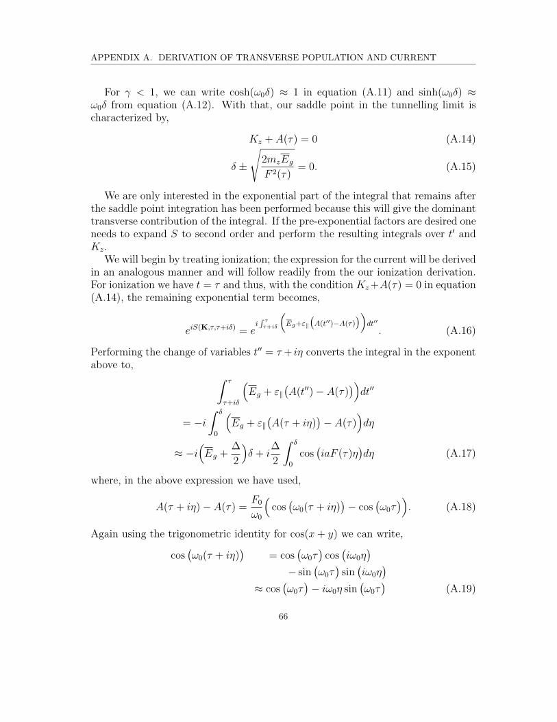
APPENDIX A. DERIVATION OF TRANSVERSE POPULATION AND CURRENT
For γ < 1, we can write cosh(ω0δ) ≈ 1 in equation (A.11) and sinh(ω0δ) ≈ω0δ from equation (A.12). With that, our saddle point in the tunnelling limit ischaracterized by,
Kz + A(τ) = 0 (A.14)
δ ±
√2mzEg
F 2(τ)= 0. (A.15)
We are only interested in the exponential part of the integral that remains afterthe saddle point integration has been performed because this will give the dominanttransverse contribution of the integral. If the pre-exponential factors are desired oneneeds to expand S to second order and perform the resulting integrals over t′ andKz.
We will begin by treating ionization; the expression for the current will be derivedin an analogous manner and will follow readily from the our ionization derivation.For ionization we have t = τ and thus, with the condition Kz+A(τ) = 0 in equation(A.14), the remaining exponential term becomes,
eiS(K,τ,τ+iδ) = ei∫ ττ+iδ
(Eg+ε‖
(A(t′′)−A(τ)
))dt′′
. (A.16)
Performing the change of variables t′′ = τ + iη converts the integral in the exponentabove to, ∫ τ
τ+iδ
(Eg + ε‖
(A(t′′)− A(τ)
))dt′′
= −i∫ δ
0
(Eg + ε‖
(A(τ + iη)
)− A(τ)
)dη
≈ −i(Eg +
∆
2
)δ + i
∆
2
∫ δ
0
cos(iaF (τ)η
)dη (A.17)
where, in the above expression we have used,
A(τ + iη)− A(τ) =F0
ω0
(cos(ω0(τ + iη)
)− cos
(ω0τ)). (A.18)
Again using the trigonometric identity for cos(x+ y) we can write,
cos(ω0(τ + iη)
)= cos
(ω0τ)
cos(iω0η
)− sin
(ω0τ)
sin(iω0η
)≈ cos
(ω0τ)− iω0η sin
(ω0τ)
(A.19)
66

APPENDIX A. DERIVATION OF TRANSVERSE POPULATION AND CURRENT
where we have approximated the terms in the first line above to first order ascos(iω0η) ≈ 1 and sin(iω0η) ≈ iω0η. Our integral can now be expressed as,∫ τ
τ+iδ
(Eg + ε‖
(A(t′′)− A(τ)
))dt′′
≈ −i(Eg + ∆
2
)δi∆
2
∫ δ0
(1 + 1
2
(azF (τ)
)2η2)dη
≈ −iEgδ + im−1z F 2(τ) δ
3
6
≈ i
√mz
(2Eg
)3/2
3F (τ)(A.20)
where, in obtaining equation (A.20) we have used the relation from equation (A.15)with the negative sign for δ and m−1
z = ∆a2z/2. Finally, inserting equation (A.20)
into the exponent and replacing F (τ) with F0 we can express the exponential partof the ionization rate as,
nc ∝∫dkxdky exp
(− 2√mz(2Eg)
3/2/3F0
). (A.21)
Taylor expanding E3/2
g gives,
E3/2
g ≈ E3/2g +
3
2
√Eg
(k2x
2mx
+k2y
2my
). (A.22)
After integration over kx,y we can split ionization into a rate n(3−q)Dc (t) that is a
combination of the longitudinal rate and the unconfined transverse term (should
one exist) and a transverse contribution nqD⊥ from the confined direction(s) that istime-independent. The population is then given by,
nc(t) =∫ t−∞ n
(3−q)Dc (t)nqD⊥ dt′
= nqD⊥∫ t−∞ n
(3−q)Dc (t)dt′
= nqD⊥ n(3−q)Dc (t) (A.23)
where nqD⊥ is given by,
nqD⊥ =
(F 2
0
2mzEg
)q/4 q∏j=1
aj
√mj
2π. (A.24)
As with the text above, q denotes the number of confined transverse directions.
67

APPENDIX A. DERIVATION OF TRANSVERSE POPULATION AND CURRENT
Turning our attention to the current, we can now write the integral in the ex-ponent as the sum of two integrals. The first runs from τ + iδ to τ and the secondruns from τ to t; this is given as,∫ t
τ+iδ
(Eg + ε‖
(A(t′′)− A(τ)
))dt′′
=
∫ τ
τ+iδ
(Eg + ε‖
(A(t′′)− A(τ)
))dt′′
+
∫ t
τ
(Eg + ε‖
(A(t′′)− A(τ)
))dt′′. (A.25)
The first integral on the right hand side is the same as that for equation (A.20).The second integral gives, ∫ t
τ
(Eg + ε‖
(A(t′′)− A(τ)
))dt′′
= Eg(t− τ) +
∫ t
τ
ε‖(A(t′′)− A(τ)
)dt′′. (A.26)
By writing the transverse band gap in the effective mass approximation we get,
Eg ≈ Eg +k2x
2mx
+k2y
2my
. (A.27)
Further, E3/2
g can be expanded as in equation (A.22) above. This allows us toexpress the 3D current j3D as,
j3D ∝∑
τ e−√mz
3F (τ)(2Eg)3/2e
i
(Eg(t−τ)+
∫ tτ ε‖
(A(t′′)−A(τ)
)dt′′
)×∏
j=x,y
√aj2π
∫∞−∞dkje
−(√
mzEg
2F20
+ i2
(t−τ)
)k2jmj (A.28)
where the summation is over all birth times τ .In a manner similar to that used to arrive at equation (3.7), the expression
in equation (A.28) can be split into an unconfined term j(3−q)D and a confined
transverse term jqD⊥ where,
|jqD⊥ |2 =
(2mzEgF 2
0
+π2
ω20
)−q/2 q∏j=1
ajmj. (A.29)
In arriving at equation (3.8), we have approximated the excursion time betweenbirth time τ and recollision time t by |t − τ | ≈ π/ω0. The exact excursion time
68

APPENDIX A. DERIVATION OF TRANSVERSE POPULATION AND CURRENT
is determined by saddle point integration of the integral resulting from the Fouriertransform of the current from time to frequency domain. For the scaling argumentdeveloped here, it is sufficient to use an excursion time is on the order of a halfcycle.
69

Appendix B
Impurity versus intrabandharmonics
The HHG spectrum in Fig. 4.4 of the main manuscript contains contributions fromboth the intraband and impurity terms. Figure B.1 compares the individual con-tributions of each of these terms. The individual harmonic spectra are calculatedby taking the absolute value squared of the Fourier transform of Eqs. (4.30) and(4.31). The harmonics generated by the impurity term are represented by the blueline and those generated by the intraband current are represented by the green line.In the above band gap range — harmonics with n ≥ 5 — the spectrum is dominatedby the impurity term by approximately 3 to 6 orders of magnitude, depending onthe harmonic. The only exception is harmonic 5 where the impurity and intrabandterms are comparable. In the below band gap regions, the impurity harmonics arethe dominant signal. The red, dashed line in the figure represent the dipole momentwhich scales similarly to the impurity harmonic signal.
We note here that the density of impurities will have an effect on the intensi-ties of the impurity and intraband harmonics. In our one-dimensional calculationswe have an impurity density of approximately 10−3 impurities per lattice cite. Inthree dimensions this density would be approximately 10−9 and will likely resultin a decrease of impurity harmonics relative to the intraband spectrum. In ourone dimensional calculations the impurity harmonics range from 3 to 6 orders-of-magnitude above the intraband harmonics. As a result, a relative impurity densityof around 10−6 corresponding to an impurity density of approximately 1016cm−3
should be sufficient to still observe stronger impurity harmonics.
Further, there is another parameter that determines the strength of impurityversus intraband HHG, which is the laser intensity. For the intraband harmonics to
70

APPENDIX B. IMPURITY VERSUS INTRABAND HARMONICS
Harmonic order
Inte
nsity
(ar
b.)
1 11 21 31 41 51 61 71
10−10
10−8
10−6
10−4
10−2
100
102
Figure B.1: The impurity (blue) and intraband (green) harmonic spectra. The red, dashed line representsthe dipole moment. The shaded area indicates the below impurity ionization potential region. The dipolehas been shifted on the y-axis to compare with the shape of the harmonic spectra.
develop, the electron must explore a significant portion of the nonlinear part of theband. Due to the low field intensities used here, the electron explores only about athird of the Brillouin zone and does not experience the full nonlinear portion of theconduction band, resulting in a reduction of the intensity of intraband harmonics.When the electron only explores a limited region of the Brillouin zone near theΓ−point, the intensity of the intraband harmonics decreases with harmonic order ata rate much larger than the impurity harmonics. The above discussion highlights theneed for careful consideration when determining doping rates and laser parameters.
71

Appendix C
Numerical solution of thetwo-band equations
The integration of Eqs. (2.11) is numerically preformed using a fourth-order Runge-Kutta method [85]. The method is a numerical technique used to solve ordinarydifferential equation of the form
y = f(y, t), (C.1)
where the initial value of y(0) = y0. At each time step, the solution is advanced asfollowing,
yn+1 = yn +h
6(k1 + 2k2 + 2k3 + k4) (C.2)
tn+1 = tn + h (C.3)
wherek1 =f(tn, yn),
k2 =f(tn +h
2, yn +
h
2k1),
k3 =f(tn +h
2, yn +
h
2k2), and
k4 =f(tn +h
2, yn + hk3).
(C.4)
To implement this method to Eqs. (2.11), we rewrite it in the form
bc,κ =iF · d∗(k)bv,κη(κ, t)
bv,κ =iF · d(k)bc,κη∗(κ, t)
η =iεg(κ)η(κ, t)
(C.5)
72

APPENDIX C. NUMERICAL SOLUTION OF THE TWO-BAND EQUATIONS
whereη(κ, t) = exp[iS(κ, t)]. (C.6)
The system of equations C.5 is solved with the following initial conditions
bv(κ, 0) =1√2kb
,
bc(κ, 0) = 0, and
η(κ, 0) = 0.
(C.7)
where kb = 2π/a is the reciprocal lattice vector and a is the lattice constant.
73

Appendix D
Atomic units and ConversionFactors
• Electron charge (e) = 1.6021× 10⁻¹⁹ C
• Electron mass (m) = 9.018× 10⁻³¹ kg
• Time = a0/v0 = ~3/me4 = 2.4189× 10⁻¹⁷s
• Length : a0 = ~2/me2 = 5.2917× 10⁻¹¹ m
• Energy = e2/a0 = 4.3597× 10⁻¹⁸J = 27.21 eV
• Velocity : v0 = e2/~ = 2.1877× 10⁶ m.s−1
• Momentum: = me2/~ = 1.9926× 10⁻²⁴ kg.m.s−1
• Freqency = v0/a0 = me4/~3 = 4.1341× 10¹⁶ s−1
• Electric potential = e/a0 = me3/~2 = 27.21 V
• Electric field strength : F0 = e/a20 = m2e5/~4 = 5.142× 10⁹ V.cm−1
74

Bibliography
[1] P. B. Corkum. Plasma perspective on strong field multiphoton ionization. Phys.Rev. Lett., 71:1994–1997, Sep 1993.
[2] P aB Corkum and Ferenc Krausz. Attosecond science. Nature physics, 3(6):381,2007.
[3] CD Lin, Anh-Thu Le, Zhangjin Chen, Toru Morishita, and Robert Lucch-ese. Strong-field rescattering physics—self-imaging of a molecule by its ownelectrons. Journal of Physics B: Atomic, Molecular and Optical Physics,43(12):122001, 2010.
[4] David N Fittinghoff, Paul R Bolton, Britton Chang, and Kenneth C Kulan-der. Observation of nonsequential double ionization of helium with opticaltunneling. Physical review letters, 69(18):2642, 1992.
[5] MB Gaarde, KJ Schafer, KC Kulander, B Sheehy, Dalwoo Kim, and LF Di-Mauro. Strong species dependence of high order photoelectron production inalkali metal atoms. Physical review letters, 84(13):2822, 2000.
[6] Barry Walker, Brian Sheehy, Kenneth C Kulander, and Louis F DiMauro.Elastic rescattering in the strong field tunneling limit. Physical review letters,77(25):5031, 1996.
[7] Benjamin Wolter, Michael G Pullen, A-T Le, Matthias Baudisch, K Doblhoff-Dier, Arne Senftleben, Michael Hemmer, C Dieter Schroter, Joachim Ullrich,Thomas Pfeifer, et al. Ultrafast electron diffraction imaging of bond breakingin di-ionized acetylene. Science, 354(6310):308–312, 2016.
[8] Shambhu Ghimire, Anthony D DiChiara, Emily Sistrunk, Pierre Agostini,Louis F DiMauro, and David A Reis. Observation of high-order harmonicgeneration in a bulk crystal. Nature physics, 7(2):138, 2011.
[9] Tran Trung Luu, M Garg, S Yu Kruchinin, Antoine Moulet, M Th Hassan,and Eleftherios Goulielmakis. Extreme ultraviolet high-harmonic spectroscopyof solids. Nature, 521(7553):498, 2015.
75

BIBLIOGRAPHY
[10] G Vampa, TJ Hammond, N Thire, BE Schmidt, F Legare, CR McDonald,T Brabec, and PB Corkum. Linking high harmonics from gases and solids.Nature, 522(7557):462, 2015.
[11] Georges Ndabashimiye, Shambhu Ghimire, Mengxi Wu, Dana A Browne, Ken-neth J Schafer, Mette B Gaarde, and David A Reis. Solid-state harmonicsbeyond the atomic limit. Nature, 534(7608):520, 2016.
[12] Ben Zaks, Ren-Bao Liu, and Mark S Sherwin. Experimental observation ofelectron–hole recollisions. Nature, 483(7391):580, 2012.
[13] Olaf Schubert, Matthias Hohenleutner, Fabian Langer, Benedikt Urbanek,C Lange, U Huttner, D Golde, T Meier, M Kira, Stephan W Koch, et al.Sub-cycle control of terahertz high-harmonic generation by dynamical blochoscillations. Nature Photonics, 8(2):119, 2014.
[14] Matthias Hohenleutner, Fabian Langer, Olaf Schubert, Matthias Knorr, U Hut-tner, SW Koch, M Kira, and Rupert Huber. Real-time observation of interferingcrystal electrons in high-harmonic generation. Nature, 523(7562):572, 2015.
[15] D. Golde, T. Meier, and S. W. Koch. High harmonics generated in semicon-ductor nanostructures by the coupled dynamics of optical inter- and intrabandexcitations. Phys. Rev. B, 77:075330, Feb 2008.
[16] G. Vampa, C. R. McDonald, G. Orlando, D. D. Klug, P. B. Corkum, andT. Brabec. Theoretical analysis of high-harmonic generation in solids. Phys.Rev. Lett., 113:073901, Aug 2014.
[17] G. Vampa, C. R. McDonald, G. Orlando, P. B. Corkum, and T. Brabec. Semi-classical analysis of high harmonic generation in bulk crystals. Phys. Rev. B,91:064302, Feb 2015.
[18] Hanzhe Liu, Yilei Li, Yong Sing You, Shambhu Ghimire, Tony F Heinz, andDavid A Reis. High-harmonic generation from an atomically thin semiconduc-tor. Nature Physics, 13(3):262, 2017.
[19] Murat Sivis, Marco Taucer, Giulio Vampa, Kyle Johnston, Andre Staudte,Andrei Yu Naumov, DM Villeneuve, Claus Ropers, and PB Corkum. Tailoredsemiconductors for high-harmonic optoelectronics. Science, 357(6348):303–306,2017.
[20] Tengfei Huang, Xiaosong Zhu, Liang Li, Xi Liu, Pengfei Lan, and Peixiang Lu.High-order-harmonic generation of a doped semiconductor. Physical Review A,96(4):043425, 2017.
76

BIBLIOGRAPHY
[21] Dejan B. Milosevic and Anthony F. Starace. Magnetic-field-induced intensityrevivals in harmonic generation. Phys. Rev. Lett., 82:2653–2656, Mar 1999.
[22] D Shafir, Y Mairesse, DM Villeneuve, PB Corkum, and N Dudovich. Atomicwavefunctions probed through strong-field light–matter interaction. NaturePhysics, 5(6):412, 2009.
[23] Serguei Patchkovskii, Zengxiu Zhao, Thomas Brabec, and DM Villeneuve. Highharmonic generation and molecular orbital tomography in multielectron sys-tems: Beyond the single active electron approximation. Physical review letters,97(12):123003, 2006.
[24] Caterina Vozzi, Matteo Negro, Francesca Calegari, Giuseppe Sansone, MauroNisoli, Sandro De Silvestri, and Salvatore Stagira. Generalized molecular or-bital tomography. Nature Physics, 7(10):822, 2011.
[25] Jiro Itatani, Jerome Levesque, Dirk Zeidler, Hiromichi Niikura, Henri Pepin,Jean-Claude Kieffer, Paul B Corkum, and David M Villeneuve. Tomographicimaging of molecular orbitals. Nature, 432(7019):867, 2004.
[26] Sarah Baker, Joseph S Robinson, CA Haworth, H Teng, RA Smith, CC Chirila,Manfred Lein, JWG Tisch, and Jonathan P Marangos. Probing proton dynam-ics in molecules on an attosecond time scale. Science, 312(5772):424–427, 2006.
[27] Hans Jakob Worner, Julien B Bertrand, Daniil V Kartashov, Paul B Corkum,and David M Villeneuve. Following a chemical reaction using high-harmonicinterferometry. Nature, 466(7306):604, 2010.
[28] Hans Jakob Worner, Julien B Bertrand, Baptiste Fabre, Julien Higuet, Hart-mut Ruf, Antoine Dubrouil, Serguei Patchkovskii, Michael Spanner, YannMairesse, Valerie Blanchet, et al. Conical intersection dynamics in no2 probedby homodyne high-harmonic spectroscopy. Science, 334(6053):208–212, 2011.
[29] A. McPherson, G. Gibson, H. Jara, U. Johann, T. S. Luk, I. A. McIntyre,K. Boyer, and C. K. Rhodes. Studies of multiphoton production of vacuum-ultraviolet radiation in the rare gases. J. Opt. Soc. Am. B, 4(4):595–601, Apr1987.
[30] M. Lewenstein, Ph. Balcou, M. Yu. Ivanov, Anne L’Huillier, and P. B. Corkum.Theory of high-harmonic generation by low-frequency laser fields. Phys. Rev.A, 49:2117–2132, Mar 1994.
[31] P. A. Franken, A. E. Hill, C. W. Peters, and G. Weinreich. Generation ofoptical harmonics. Phys. Rev. Lett., 7:118–119, Aug 1961.
77

BIBLIOGRAPHY
[32] Thomas Brabec and Ferenc Krausz. Intense few-cycle laser fields: Frontiers ofnonlinear optics. Rev. Mod. Phys., 72:545–591, Apr 2000.
[33] Robert W Boyd. Nonlinear optics. Elsevier, 2003.
[34] Peter Hawkins. High harmonic generation in periodic systems. 2016.
[35] Ryuji Morita and Mikio Yamashita. Relationship between second-and third-order nonlinear optical susceptibilities due to electronic polarization. Japanesejournal of applied physics, 32(7A):L905, 1993.
[36] N. H. Burnett, H. A. Baldis, M. C. Richardson, and G. D. Enright. Harmonicgeneration in co2 laser target interaction. Applied Physics Letters, 31(3):172–174, 1977.
[37] LV Keldysh et al. Ionization in the field of a strong electromagnetic wave. Sov.Phys. JETP, 20(5):1307–1314, 1965.
[38] MV Ammosov. Mv ammosov, nb delone, and vp krainov, sov. phys. jetp 64,1191 (1986). Sov. Phys. JETP, 64:1191, 1986.
[39] Jeffrey L. Krause, Kenneth J. Schafer, and Kenneth C. Kulander. High-orderharmonic generation from atoms and ions in the high intensity regime. Phys.Rev. Lett., 68:3535–3538, Jun 1992.
[40] K. J. Schafer, Baorui Yang, L. F. DiMauro, and K. C. Kulander. Above thresh-old ionization beyond the high harmonic cutoff. Phys. Rev. Lett., 70:1599–1602,Mar 1993.
[41] T Pfeifer, Ch Spielmann, and G Gerber. Femtosecond x-ray science. Reportson Progress in Physics, 69(2):443, 2006.
[42] Charles G. Durfee, Andy R. Rundquist, Sterling Backus, Catherine Herne,Margaret M. Murnane, and Henry C. Kapteyn. Phase matching of high-orderharmonics in hollow waveguides. Phys. Rev. Lett., 83:2187–2190, Sep 1999.
[43] Misha Yu Ivanov, Thomas Brabec, and Neal Burnett. Coulomb corrections andpolarization effects in high-intensity high-harmonic emission. Physical ReviewA, 54(1):742, 1996.
[44] See Leang Chin, Pierre Agostini, and Gaetano Ferrante. Progress in UltrafastIntense Laser Science III, volume 89. Springer Science & Business Media, 2008.
[45] NW Ashcroft and ND Mermin. Solid state physics; thomson learning, inc.Stamford, CT, 1976.
78

BIBLIOGRAPHY
[46] F Brunel. Harmonic generation due to plasma effects in a gas undergoingmultiphoton ionization in the high-intensity limit. JOSA B, 7(4):521–526, 1990.
[47] Hartmut Haug and Stephan W Koch. Quantum Theory of the Optical andElectronic Properties of Semiconductors. WORLD SCIENTIFIC, 5th edition,2009.
[48] C. R. McDonald, G. Vampa, P. B. Corkum, and T. Brabec. Interband blochoscillation mechanism for high-harmonic generation in semiconductor crystals.Phys. Rev. A, 92:033845, Sep 2015.
[49] Paul Harrison and Alex Valavanis. Quantum wells, wires and dots: theoreticaland computational physics of semiconductor nanostructures. John Wiley &Sons, 2016.
[50] Peter G. Hawkins, Misha Yu. Ivanov, and Vladislav S. Yakovlev. Effect ofmultiple conduction bands on high-harmonic emission from dielectrics. Phys.Rev. A, 91:013405, Jan 2015.
[51] Mengxi Wu, Shambhu Ghimire, David A. Reis, Kenneth J. Schafer, andMette B. Gaarde. High-harmonic generation from bloch electrons in solids.Phys. Rev. A, 91:043839, Apr 2015.
[52] I Vurgaftman, J aR Meyer, and L aR Ram-Mohan. Band parameters foriii–v compound semiconductors and their alloys. Journal of applied physics,89(11):5815–5875, 2001.
[53] U Ozgur, Ya I Alivov, Chunli Liu, A Teke, MA Reshchikov, S Dogan, VCSJAvrutin, S-J Cho, and H Morkoc. A comprehensive review of zno materialsand devices. Journal of applied physics, 98(4):11, 2005.
[54] A Schleife, F Fuchs, C Rodl, J Furthmuller, and F Bechstedt. Band-structureand optical-transition parameters of wurtzite mgo, zno, and cdo from quasi-particle calculations. physica status solidi (b), 246(9):2150–2153, 2009.
[55] Qimin Yan, Patrick Rinke, Momme Winkelnkemper, Abdallah Qteish, DieterBimberg, Matthias Scheffler, and Chris G Van de Walle. Strain effects and bandparameters in mgo, zno, and cdo. Applied Physics Letters, 101(15):152105,2012.
[56] CR McDonald, G Vampa, PB Corkum, and T Brabec. Intense-laser solidstate physics: unraveling the difference between semiconductors and dielectrics.Physical review letters, 118(17):173601, 2017.
79

BIBLIOGRAPHY
[57] Martin Schultze, Krupa Ramasesha, CD Pemmaraju, SA Sato, D Whitmore,A Gandman, James S Prell, LJ Borja, D Prendergast, K Yabana, et al. At-tosecond band-gap dynamics in silicon. Science, 346(6215):1348–1352, 2014.
[58] Martin Schultze, Elisabeth M Bothschafter, Annkatrin Sommer, SimonHolzner, Wolfgang Schweinberger, Markus Fiess, Michael Hofstetter, ReinhardKienberger, Vadym Apalkov, Vladislav S Yakovlev, et al. Controlling dielectricswith the electric field of light. Nature, 493(7430):75, 2013.
[59] Agustin Schiffrin, Tim Paasch-Colberg, Nicholas Karpowicz, Vadym Apalkov,Daniel Gerster, Sascha Muhlbrandt, Michael Korbman, Joachim Reichert, Mar-tin Schultze, Simon Holzner, et al. Optical-field-induced current in dielectrics.Nature, 493(7430):70, 2013.
[60] Annkatrin Sommer, EM Bothschafter, SA Sato, Clemens Jakubeit, TobiasLatka, Olga Razskazovskaya, Hanieh Fattahi, Michael Jobst, W Schweinberger,Vage Shirvanyan, et al. Attosecond nonlinear polarization and light–matter en-ergy transfer in solids. Nature, 534(7605):86, 2016.
[61] Takuya Higuchi, Christian Heide, Konrad Ullmann, Heiko B Weber, and PeterHommelhoff. Light-field-driven currents in graphene. Nature, 550(7675):224,2017.
[62] Yong Sing You, David A Reis, and Shambhu Ghimire. Anisotropic high-harmonic generation in bulk crystals. Nature Physics, 13(4):345, 2017.
[63] II EN Adams. Motion of an electron in a perturbed periodic potential. PhysicalReview, 85(1):41, 1952.
[64] Joaquin M Luttinger and Walter Kohn. Motion of electrons and holes in per-turbed periodic fields. Physical Review, 97(4):869, 1955.
[65] W Kohn and JM Luttinger. Hyperfine splitting of donor states in silicon.Physical Review, 97(4):883, 1955.
[66] Sokrates T Pantelides. The electronic structure of impurities and other pointdefects in semiconductors. Reviews of Modern Physics, 50(4):797, 1978.
[67] Xiao-Min Tong, ZX Zhao, and Chii-Dong Lin. Theory of molecular tunnelingionization. Physical Review A, 66(3):033402, 2002.
[68] Tengfei Luo, Jivtesh Garg, Junichiro Shiomi, Keivan Esfarjani, and Gang Chen.Gallium arsenide thermal conductivity and optical phonon relaxation timesfrom first-principles calculations. EPL (Europhysics Letters), 101(1):16001,2013.
80

BIBLIOGRAPHY
[69] Yasushi Shinohara, Kazuhiro Yabana, Yosuke Kawashita, J-I Iwata, TomohitoOtobe, and George F Bertsch. Coherent phonon generation in time-dependentdensity functional theory. Physical Review B, 82(15):155110, 2010.
[70] Muneaki Hase, Masayuki Katsuragawa, Anca Monia Constantinescu, andHrvoje Petek. Frequency comb generation at terahertz frequencies by coherentphonon excitation in silicon. Nature photonics, 6(4):243, 2012.
[71] BK Meyer, J Sann, DM Hofmann, C Neumann, and A Zeuner. Shallow donorsand acceptors in zno. Semiconductor Science and Technology, 20(4):S62, 2005.
[72] Matthias C Hoffmann and Jozsef Andras Fulop. Intense ultrashort terahertzpulses: generation and applications. Journal of Physics D: Applied Physics,44(8):083001, 2011.
[73] Ml J Caldas, A Fazzio, and Alex Zunger. A universal trend in the bind-ing energies of deep impurities in semiconductors. Applied Physics Letters,45(6):671–673, 1984.
[74] W Boutu, Stefan Haessler, H Merdji, P Breger, G Waters, M Stankiewicz,LJ Frasinski, R Taieb, J Caillat, A Maquet, et al. Coherent control of attosec-ond emission from aligned molecules. Nature Physics, 4(7):545, 2008.
[75] VE Gruzdev. Photoionization rate in wide band-gap crystals. Physical ReviewB, 75(20):205106, 2007.
[76] PA Zhokhov and AM Zheltikov. Field-cycle-resolved photoionization in solids.Physical review letters, 113(13):133903, 2014.
[77] PA Zhokhov and AM Zheltikov. Depth-resolved subcycle dynamics of pho-toionization in solids. Physical Review A, 96(3):033415, 2017.
[78] Vitaly Gruzdev and Olga Sergaeva. Ultrafast modification of band structure ofwide-band-gap solids by ultrashort pulses of laser-driven electron oscillations.Physical Review B, 98(11):115202, 2018.
[79] G Vampa. G. vampa, tj hammond, n. thire, be schmidt, f. legare, cr mcdonald,t. brabec, dd klug, and pb corkum, phys. rev. lett. 115, 193603 (2015). Phys.Rev. Lett., 115:193603, 2015.
[80] Shicheng Jiang, Jigen Chen, Hui Wei, Chao Yu, Ruifeng Lu, and CD Lin. Roleof the transition dipole amplitude and phase on the generation of odd andeven high-order harmonics in crystals. Physical Review Letters, 120(25):253201,2018.
81

BIBLIOGRAPHY
[81] Keliang He, Nardeep Kumar, Liang Zhao, Zefang Wang, Kin Fai Mak, HuiZhao, and Jie Shan. Tightly bound excitons in monolayer wse 2. Physicalreview letters, 113(2):026803, 2014.
[82] Alexey Chernikov, Timothy C Berkelbach, Heather M Hill, Albert Rigosi, YileiLi, Ozgur Burak Aslan, David R Reichman, Mark S Hybertsen, and Tony FHeinz. Exciton binding energy and nonhydrogenic rydberg series in monolayerws 2. Physical review letters, 113(7):076802, 2014.
[83] Isabella Floss, Christoph Lemell, Georg Wachter, Valerie Smejkal, Shunsuke A.Sato, Xiao-Min Tong, Kazuhiro Yabana, and Joachim Burgdorfer. Ab initiomultiscale simulation of high-order harmonic generation in solids. Phys. Rev.A, 97:011401, Jan 2018.
[84] Paul M Koenraad and Michael E Flatte. Single dopants in semiconductors.Nature materials, 10(2):91, 2011.
[85] David Kincaid, David Ronald Kincaid, and Elliott Ward Cheney. Numericalanalysis: mathematics of scientific computing, volume 2. American Mathemat-ical Soc., 2009.
82