Ultrafast tutorial in Ultrafast Magnetism

Richard F L Evans

richard.evans@york.ac.ukwww-users.york.ac.uk/~rfle500/

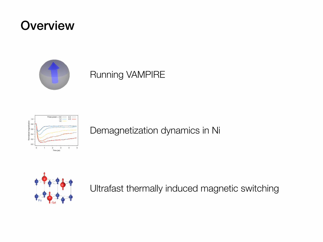
Overview

Running VAMPIRE

Demagnetization dynamics in Ni

Ultrafast thermally induced magnetic switching

0.0

0.2

0.4

0.6

0.8

1.0

0 1 2 3 4 5

No

rma

lize

d m

ag

ne

tiza

tion

Time (ps)

Pulse power = 0.81.21.6

2.22.6

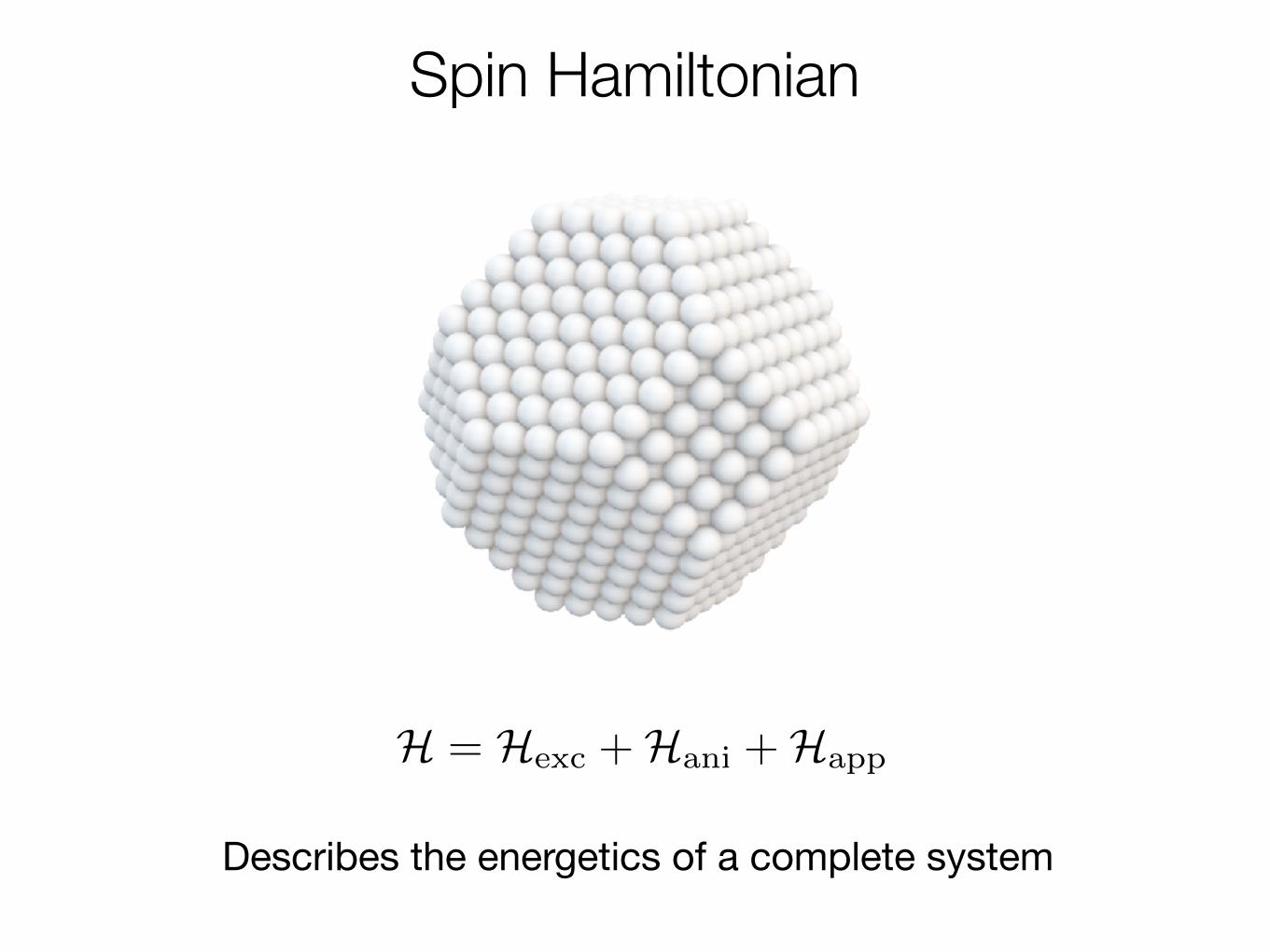
Spin Hamiltonian

Describes the energetics of a complete system

2

II. THE ATOMISTIC SPIN MODEL

Magnetism on the atomic scale presents two naturallimits: the discrete limit of continuum micromagneticsand the classical limit for the quantum mechanical elec-tron spin. The essential model of atomic scale magnetismwas devised by Heisenberg in 192824 for molecular hy-drogen. The so-named Heisenberg model describes theatomic scale exchange interaction with a local momenttheory, considering the interaction between two electronspins on neighbouring atomic sites. By applying theHeitler-London approximation25 for the linear combina-tion of electron orbitals, Heisenberg developed a modelwhich describes the energy of neighbouring atoms withspin, given by:

< H >= �JijSi · Sj (1)

where Si and Sj are the quantum mechanical spins onatomic sites i and j respectively, and Jij is the interactionenergy arising from the probability of the two electronsexchanging atomic sites. The quantum mechanical na-ture of the electron spins leads to quantization of the elec-tron energy, which for a single spin was demonstrated bythe Stern-Gerlach experiment26. In the above case, how-ever, the quantum e↵ects are far more complex due to thecoupling of the electronic spin moments. In the limit ofinfinite spin angular momentum, the quantisation e↵ectsvanish, and the spin moments have continuous degrees offreedom. Such spins are said to be classical, leading tothe classical Heisenberg spin model. It should be pointedout that there is a fundamental assumption within theHeisenberg model, namely that the electrons are closelybound to the atomic sites. In general this is not the casefor most magnetic materials, since the magnetic interac-tions usually arise from unpaired outer electrons, whichin metals are loosely bound. The band theory of fer-romagnetism proposed by Stoner27 successfully explainswhy the usual magnetic atoms possess non-integer spinmoments by describing the exchange splitting of the spin-up and spin-down energy bands. However, the band the-ory reveals little about the fundamental magnetic prop-erties due to its complexity, and so an assumption thaton some, very short, timescale the local moment approx-imation is valid is not unreasonable, provided that itis acknowledged that in fact electrons are not confinedto the atomic sites over longer timescales. Collectivelythis leads to an e↵ective Heisenberg classical spin model,where the spins have some non-integer, time-averaged,value of the spin moment which is assumed constant.Discussion, Hubbard model

A. The Classical Spin Hamiltonian

The Heisenberg spin model incorporates all the pos-sible magnetic interactions into a single convenient for-

malism which can be used to investigate a myriad ofmagnetic phenomena at the natural atomic scale. Theprincipal component of the model is the formation of thespin Hamiltonian, describing the fundamental energeticsof any magnetic system. Such a Hamiltonian is formedfrom a summation of contributions, each of which de-scribes an interaction between an atomic spin momentand neighbouring moments or external magnetic fields.The spin Hamiltonian typically takes the form:

H = Hexc +Hani +Happ (2)

The dominant contribution to the spin Hamiltonian forthe vast majority of magnetic materials comes from theexchange or Weiss field, which attempts to align theatomic spin moments. The Weiss field in fact originatesfrom the quantum mechanical exchange interaction, aris-ing from the probability of an electron moving from oneatomic site to another. The exchange interaction, as it iscalled, leads to very strong alignment of spin moments totheir neighbours in ferromagnetic metals. The total ex-change energy for each atom, i, is described by the sumover all neighbouring atomic spin moments:

Hexchange =X

i<j

JijSi · Sj (3)

where Jij is the exchange interaction between the sites iand j, Si is the local spin moment and Sj are the spinmoments of neighbouring atoms. The spin moments areexpressed here as unit vectors Si = µi/|µi|. In the sim-plest case the exchange interaction is single valued, andthe interaction is only between nearest neighbours. Inthis case a negative value of Jij results in a ferromagneticinteraction between spins and attempts to align the spins,while a positive value results in an anti-ferromagneticinteraction between spins, which attempts to align thespins anti-parallel. In more complex materials, the ex-change interaction forms a tensor with components:

Jij =

2

4Jxx Jxy Jxz

Jyx Jyy Jyz

Jzx Jzy Jzz

3

5 (4)

which is capable of describing anisotropic exchange in-teractions, such as two-ion anisotropy (Oleg) and theDzyaloshinskii-Moriya interaction (o↵-diagonal compo-nents of the exchange tensor). Additionally the exchangeinteraction can extend to several atomic spacings, rep-resenting hundreds of atomic interactions. Such com-plex interactions generally result from Density FunctionalTheory parameterisation of magnetic materials, wherethe electronic interactions can extend far away from thelocal spin.

After the exchange interaction, the most important pa-rameter in a magnetic system is generally the magneto-crystalline anisotropy, namely the preference for spin mo-ments to align with particular crystallographic axes, aris-ing from the e↵ect of the local crystal environment on

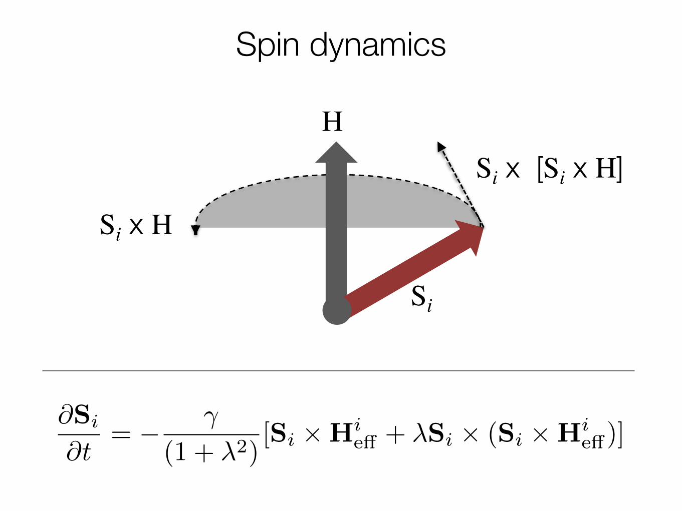
Spin dynamics

Si

HSi x [Si x H]

Si x H

5

Anisotropy energy

The atomistic magnetocrystalline anisotropy ku is de-rived from the macroscopic anisotropy constant Ku bythe expression:

ku =Kua

3

nat(10)

where Ku in given in J/m3. In addition to the atom-istic parameters, it is also worth noting the analogousexpressions for the anisotropy field Ha for a single do-main particle:

Ha =2Ku

Ms=

2kuµs

(11)

where symbols have their usual meaning.

Temperature dependent Hc?

Applying the preceding operations, parameters for thekey ferromagnetic elements are given in Tab. III.

Ferrimagnets and antiferromagnets

In the case of ferrimagnets and anti-ferromagnets theabove methods for anisotropy and moment determina-tion do not work due to the lack of macroscopic measure-ments, although the estimated exchange energies applyequally well to the Neel temperature provided no mag-netic frustration (due to lattice symmetry) is present.In general, other theoretical calculations or formalismsare required to determine parameters, such as mean-fieldapproaches1 or density functional theory calculations20.

Atomistic System Generation

Besides providing a comprehensive collection of meth-ods for the simulation of magnetic materials, another keycomponent of the vampire software package is the abil-ity to generate and model a wide variety of systems, in-cluding single crystals, thin films, multilayers, nanopar-ticles, core-shell systems and granular films. In additionto these structural parameters each system may compriseseveral di↵erent materials, each with a distinct set of ma-terial properties such as exchange, anisotropy and mag-netic moments. This naturally allows the simulation ofalloys at the atomic level and atomistic details such asinterface roughness and intermixing. In addition to thebuilt-in system generation, vampire can also import anyarbitrary set of atomic positions and interactions allow-ing to to deal with almost any kind of magnetic structure.However in the following we shall restrict ourselves to thegeneration of a generic system with nearest neighbor in-teractions only.

The first step is to generate a crystal lattice of thedesired type and dimensions su�ciently large to incorpo-rate the complete system. vampire uses the unit cell asthe essential building block of the atomic structure, sincethe exchange interactions of atoms between neighboringunit cells are known before the structure is generated.The global crystal is generated by replicating the basicunit cell on a grid in x,y and z.This bare crystal structure is then cut into the de-

sired geometry, for example a single nanoparticle, voronoigranular structure, or a user defined 2D geometry byremoving atoms from the complete generated crystal.Atoms within this geometry are then assigned to oneor more materials as desired, generating the completeatomic system.The final step is determining the exchange interactions

for all atoms in the defined system. Since each cell on thegrid contains a fixed number of atoms, and the exchangeinteractions of those atoms with other neighboring cellsis known relative to the local cell, the interaction list istrivial to generate. For computational e�ciency the finalinteraction list is then stored as a linked list, completingthe setup of the atomistic system ready for integration.parallel implementation.

IV. INTEGRATION METHODS

Although the spin Hamiltonian describes the energet-ics of the magnetic system, it provides no informationregarding its time evolution, thermal fluctuations, or theability to determine the ground state for the system. Inthe following the commonly utilized integration methodsfor atomistic spin models are introduced.

Spin Dynamics

The first understanding of spin dynamics came fromferromagnetic resonance experiments, where the time de-pendent behavior of a magnetic materials is describedby the equation derived by Landau and Lifshitz31. Thephenomenological damping parameter ↵ in the Landau-Lifshitz equation describes the coupling of the magneti-zation to the heat bath causing relaxation of the magne-tization toward the applied field direction. In the firstapproximation the relaxation rate was assumed a lin-ear function of the damping parameter. SubsequentlyGilbert introduced a critical damping parameter, with amaximum e↵ective damping for � = 1, to arrive at theLandau-Lifshitz-Gilbert (LLG) equation32.The modern form of the LLG at the atomistic level is

given by:

@Si

@t= �

�

(1 + �2)[Si ⇥H

ie↵ + �Si ⇥ (Si ⇥H

ie↵)] (12)

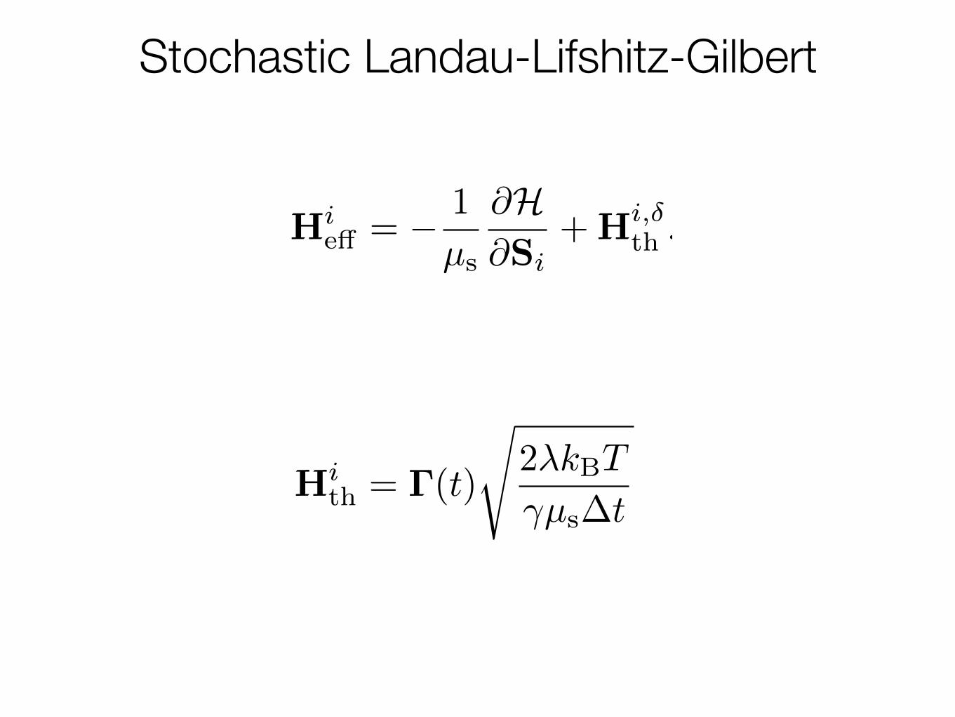
Stochastic Landau-Lifshitz-Gilbert

6

TABLE III. Table of derived constants for the ferromagnetic elements Fe, Co and Ni.

Fe Co Ni UnitCrystal structure BCC HCP FCC -Unit cell size a 2.5 2.5 2.5 ACoordination number z 8 12 12 -Curie Temperature Tc 1043 1388 600 KAtomic spin moment µs 2.2 1.44 0.6 µB

Exchange Energy Jij 4.5 ⇥10�21 4.5 ⇥10�21 5.6 ⇥10�21 J/linkAnisotropy Energy ku 4.5 ⇥10�26 4.5 ⇥10�24 4.5 ⇥10�25 J/atom

where Si is a unit vector representing the direction of themagnetic spin moment of site i, � is the gyromagnetic ra-tio, � is the Gilbert damping parameter, and H

ie↵ is the

net magnetic field on each spin. The LLG equation de-scribes the interaction of an atomic spin moment i withan e↵ective magnetic field, which is obtained from thenegative first derivative of the complete spin Hamilto-nian, such that:

Hie↵ = �

1

µs

@H

@Si(13)

where µs is the local spin moment. The inclusion of thespin moment within the e↵ective field is significant, inthat the field is then expressed in units of Tesla, givena Hamiltonian in Joules. Given typical energies in theHamiltonian of 10 µeV - 100 meV range. This gives fieldstypically in the range 0.1 - 1000 Tesla, given a spin mo-ment of the same order as the Bohr magneton (µB).

The LLG equation has two distinct parts, the first part,Si ⇥H

ie↵ induces spin precession around the net field di-

rection Hie↵ , while the second, �Si⇥(Si⇥H

ie↵) describes

spin relaxation towards Hie↵ . The phenomenological mi-

croscopic damping constant, �, determines the rate ofrelaxation towards the net field direction, representingthe coupling of the spin system to a heat bath. It shouldbe noted that the intrinsic damping � is di↵erent to theextrinsic damping ↵ measured experimentally. The in-trinsic damping arises due to microscopic e↵ects suchas spin-lattice33 and electron-spin interactions34, whilethe macroscopic damping ↵ has additional contributionsfrom temperature, disorder, defects, and magnetostaticinteractions.

Langevin Dynamics

In its standard form the LLG equation is strictly onlyapplicable to simulations at zero temperature. Ther-mal e↵ects cause thermodynamic fluctuations of the spinmoments which at su�ciently high temperatures arestronger than the exchange interaction and giving riseto the ferromagnetic-paramagnetic transition. The ef-fects of temperature can be taken into account by usingLangevin Dynamics, an approach developed by Brown35.

The basic idea behind Langevin Dynamics is to assumethat the thermal fluctuations on each atomic site canbe represented by a Gaussian white noise term. As thetemperature is increased, the width of the Gaussian dis-tribution increases, thus representing stronger thermalfluctuations. In reality the thermal and magnetic fluctu-ations are correlated at the atomic level, arising from thedynamic interactions between the atoms and electrons.New approaches such as colored noise36 and combinedmagnetic and molecular dynamics simulations37,38 aimto better understand the underlying physics of the ther-mal interactions at the atomic level.

Nevertheless the established Langevin Dynamicsmethod is widely used for spin dynamics simulations andincorporates an e↵ective thermal field into the LLG equa-tion to simulate thermal e↵ects39–41. The thermal fluctu-ations are represented by a gaussian distribution �(t) inthree dimensions with a mean of zero. At each time stepthe instantaneous thermal field on each spin i is given by:

Hith = �(t)

s2�kBT

�µs�t(14)

where kB is the Boltzmann constant, T is the systemtemperature, � is the Gilbert damping parameter, � isthe absolute value of the gyromagnetic ratio, µs is themagnitude of the atomic magnetic moment, and�t is theintegration time step. The e↵ective field for applicationin the LLG equation with Langevin Dynamics then reads:

Hie↵ = �

1

µs

@H

@Si+H

i,�th . (15)

Given that for each time step three Gaussian dis-tributed random numbers are required for every spin, ef-ficient generation of such numbers is essential. vampiretherefore makes use the Mersenne Twister42 uniform ran-dom number generator and the Ziggurat method43 forgenerating the Gaussian distribution.

6

TABLE III. Table of derived constants for the ferromagnetic elements Fe, Co and Ni.

Fe Co Ni UnitCrystal structure BCC HCP FCC -Unit cell size a 2.5 2.5 2.5 ACoordination number z 8 12 12 -Curie Temperature Tc 1043 1388 600 KAtomic spin moment µs 2.2 1.44 0.6 µB

Exchange Energy Jij 4.5 ⇥10�21 4.5 ⇥10�21 5.6 ⇥10�21 J/linkAnisotropy Energy ku 4.5 ⇥10�26 4.5 ⇥10�24 4.5 ⇥10�25 J/atom

where Si is a unit vector representing the direction of themagnetic spin moment of site i, � is the gyromagnetic ra-tio, � is the Gilbert damping parameter, and H

ie↵ is the

net magnetic field on each spin. The LLG equation de-scribes the interaction of an atomic spin moment i withan e↵ective magnetic field, which is obtained from thenegative first derivative of the complete spin Hamilto-nian, such that:

Hie↵ = �

1

µs

@H

@Si(13)

where µs is the local spin moment. The inclusion of thespin moment within the e↵ective field is significant, inthat the field is then expressed in units of Tesla, givena Hamiltonian in Joules. Given typical energies in theHamiltonian of 10 µeV - 100 meV range. This gives fieldstypically in the range 0.1 - 1000 Tesla, given a spin mo-ment of the same order as the Bohr magneton (µB).

The LLG equation has two distinct parts, the first part,Si ⇥H

ie↵ induces spin precession around the net field di-

rection Hie↵ , while the second, �Si⇥(Si⇥H

ie↵) describes

spin relaxation towards Hie↵ . The phenomenological mi-

croscopic damping constant, �, determines the rate ofrelaxation towards the net field direction, representingthe coupling of the spin system to a heat bath. It shouldbe noted that the intrinsic damping � is di↵erent to theextrinsic damping ↵ measured experimentally. The in-trinsic damping arises due to microscopic e↵ects suchas spin-lattice33 and electron-spin interactions34, whilethe macroscopic damping ↵ has additional contributionsfrom temperature, disorder, defects, and magnetostaticinteractions.

Langevin Dynamics

In its standard form the LLG equation is strictly onlyapplicable to simulations at zero temperature. Ther-mal e↵ects cause thermodynamic fluctuations of the spinmoments which at su�ciently high temperatures arestronger than the exchange interaction and giving riseto the ferromagnetic-paramagnetic transition. The ef-fects of temperature can be taken into account by usingLangevin Dynamics, an approach developed by Brown35.

The basic idea behind Langevin Dynamics is to assumethat the thermal fluctuations on each atomic site canbe represented by a Gaussian white noise term. As thetemperature is increased, the width of the Gaussian dis-tribution increases, thus representing stronger thermalfluctuations. In reality the thermal and magnetic fluctu-ations are correlated at the atomic level, arising from thedynamic interactions between the atoms and electrons.New approaches such as colored noise36 and combinedmagnetic and molecular dynamics simulations37,38 aimto better understand the underlying physics of the ther-mal interactions at the atomic level.

Nevertheless the established Langevin Dynamicsmethod is widely used for spin dynamics simulations andincorporates an e↵ective thermal field into the LLG equa-tion to simulate thermal e↵ects39–41. The thermal fluctu-ations are represented by a gaussian distribution �(t) inthree dimensions with a mean of zero. At each time stepthe instantaneous thermal field on each spin i is given by:

Hith = �(t)

s2�kBT

�µs�t(14)

where kB is the Boltzmann constant, T is the systemtemperature, � is the Gilbert damping parameter, � isthe absolute value of the gyromagnetic ratio, µs is themagnitude of the atomic magnetic moment, and�t is theintegration time step. The e↵ective field for applicationin the LLG equation with Langevin Dynamics then reads:

Hie↵ = �

1

µs

@H

@Si+H

i,�th . (15)

Given that for each time step three Gaussian dis-tributed random numbers are required for every spin, ef-ficient generation of such numbers is essential. vampiretherefore makes use the Mersenne Twister42 uniform ran-dom number generator and the Ziggurat method43 forgenerating the Gaussian distribution.

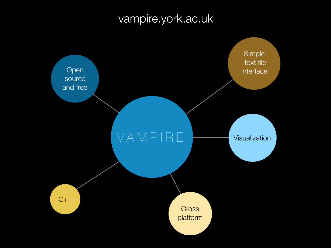
Open source

and free

C++

V A M P I R E

Simple text file interface

Visualization

Cross platform

vampire.york.ac.uk

Tutorial resources

www-users.york.ac.uk/~rfle500/teaching/ultrafast-magnetism/

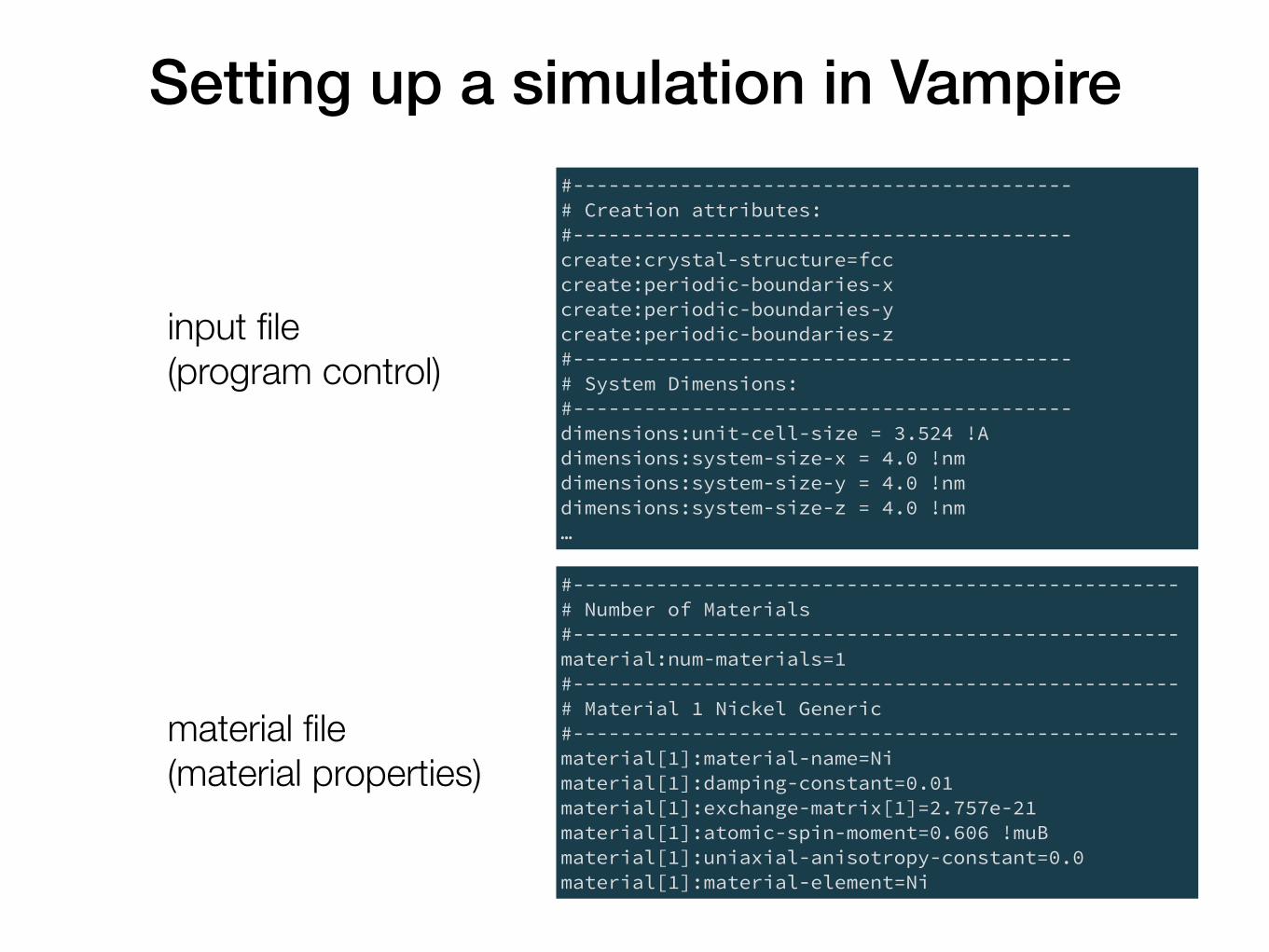
Setting up a simulation in Vampire

input file (program control)

material file (material properties)

#------------------------------------------ # Creation attributes: #------------------------------------------ create:crystal-structure=fcc create:periodic-boundaries-x create:periodic-boundaries-y create:periodic-boundaries-z #------------------------------------------ # System Dimensions: #------------------------------------------ dimensions:unit-cell-size = 3.524 !A dimensions:system-size-x = 4.0 !nm dimensions:system-size-y = 4.0 !nm dimensions:system-size-z = 4.0 !nm …

#--------------------------------------------------- # Number of Materials #--------------------------------------------------- material:num-materials=1 #--------------------------------------------------- # Material 1 Nickel Generic #--------------------------------------------------- material[1]:material-name=Ni material[1]:damping-constant=0.01 material[1]:exchange-matrix[1]=2.757e-21 material[1]:atomic-spin-moment=0.606 !muB material[1]:uniaxial-anisotropy-constant=0.0 material[1]:material-element=Ni

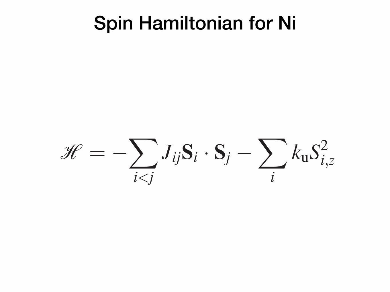
Spin Hamiltonian for Ni

Ultrafast thermally induced magnetic switching in synthetic ferrimagnets

Richard F. L. Evans,1,a) Thomas A. Ostler,1 Roy W. Chantrell,1 Ilie Radu,2 and Theo Rasing3

1Department of Physics, University of York, Heslington, York YO10 5DD, United Kingdom2Institut f€ur Methoden und Instrumentierung der Forschung mit Synchrotronstrahlung, Helmholtz-ZentrumBerlin f€ur Materialien und Energie GmbH, Albert-Einstein-Straße 15, 12489 Berlin, Germany3Radboud University, Institute for Molecules and Materials, Heyendaalsewg 135, 6525 AJ Nijmegen,The Netherlands

(Received 19 October 2013; accepted 10 February 2014; published online 27 February 2014)

Synthetic ferrimagnets are composite magnetic structures formed from two or more anti-ferromagnetically coupled magnetic sublattices with different magnetic moments. Here, wereport on atomistic spin simulations of the laser-induced magnetization dynamics on suchsynthetic ferrimagnets and demonstrate that the application of ultrashort laser pulses leads tosub-picosecond magnetization dynamics and all-optical switching in a similar manner as inferrimagnetic alloys. Moreover, we present the essential material properties for successful laser-induced switching, demonstrating the feasibility of using a synthetic ferrimagnet as a highdensity magnetic storage element without the need of a write field. VC 2014 AIP Publishing LLC.[http://dx.doi.org/10.1063/1.4867015]

The dynamic response of magnetic materials to ultra-short laser pulses is currently an area of fundamental andpractical importance that is attracting a lot of attention. Sincethe pioneering work of Beaurepaire et al.,1 it has been knownthat the magnetization can respond to a femtosecond laserpulse on a sub-picosecond timescale. However, studies ofmagnetic switching are more recent. In this context, an espe-cially intriguing phenomenon is that of all-optical switching,which uses the interaction of short, intense pulses of lightwith a magnetic material to alter its magnetic state withoutthe application of an external magnetic field.2,3 Recentexperiments4– 6 and theoretical calculations5,7– 9 have demon-strated that the origin of all-optical switching in ferrimagneticalloys is due to ultrafast heating of the spin system. The mag-netic switching arises due to a transfer of angular momentumbetween the two sublattices within the material7,8 and theresulting exchange-field induced precession.7 Remarkably,this effect occurs in the absence of any symmetry breakingmagnetic field,5 and can be considered as Thermally InducedMagnetic Switching (TIMS). So far, TIMS has only beendemonstrated experimentally in the rare-earth transition metal(RE-TM) alloys GdFeCo and TbCo which, in addition totheir strong magneto-optical response, have two essentialproperties for heat-induced switching: antiferromagnetic cou-pling between the RE and TM sublattices10 and distinctdemagnetization times of the two sublattices.4 The antiferro-magnetic coupling allows for inertial magnetization dynam-ics, while the distinct demagnetization times under the actionof a heat pulse allow a transient imbalance in the angular mo-mentum of the two sublattices, which initiates a mutual highspeed precession enabling ultrafast switching to occur.

Although GdFeCo has excellent switching properties, itspotential use in magnetic data storage is limited by its low an-isotropy and amorphous structure, precluding the use of sin-gle magnetic domains typically less than 10 nm in size,required for future high density magnetic recording media.

One intriguing possibility, and the focus of this paper, wouldbe the use of a synthetic ferrimagnet (SFiM), consisting oftwo transition metal ferromagnets anti-ferromagneticallyexchange coupled by a non-magnetic spacer,11 shown sche-matically in Fig. 1. The important but as yet unansweredquestion is whether all-optical switching would also work insuch an artificial structure and what essential physical proper-ties of the design are required. Such a composite magnet alsohas a number of distinct advantages over intrinsic rare-earth-transition metal ferrimagnets: the dynamic properties of eachsublattice may be separately selected by choice of material,nano-patterning is possible in the sub-10 nm size range due totheir crystalline nature and the omission of costly rare-earthmetals. Importantly the composite design has the advantageof allowing the use of high anisotropy materials such as FePtor CoPt to enhance the thermal stability of the medium.These advantages could make such synthetic structures verypromising candidates for magnetic data storage applications.

In this Letter we present dynamic studies of such a syn-thetic ferrimagnet using an atomistic spin model. We investi-gate the dynamic properties of the separate layers and showthat the demagnetization time is determined primarily by thelocal atomic spin moment and the intrinsic Gilbert dampingof the material. We finally consider an exchange-coupledFe/FePt synthetic ferrimagnet and show that a short heat-pulse is sufficient to induce ultrafast heat-induced switchingof the material.

The dynamic properties of the SFiM are studied using anatomistic spin model using the VAMPIRE software package.12,13

The energetics of the system are described using aHeisenberg spin Hamiltonian, which in condensed form reads

H ¼ "X

i<j

JijSi # Sj "X

i

kuS2i;z; (1)

where Jij is the exchange energy between nearest neighboringspins, Si and Sj are unit vectors describing the spin directionsfor local sites i and nearest neighbor sites j, respectively, andku is the uniaxial anisotropy constant. There are three distincta)richard.evans@york.ac.uk

0003-6951/2014/104(8)/082410/4/$30.00 VC 2014 AIP Publishing LLC104, 082410-1

APPLIED PHYSICS LETTERS 104, 082410 (2014)

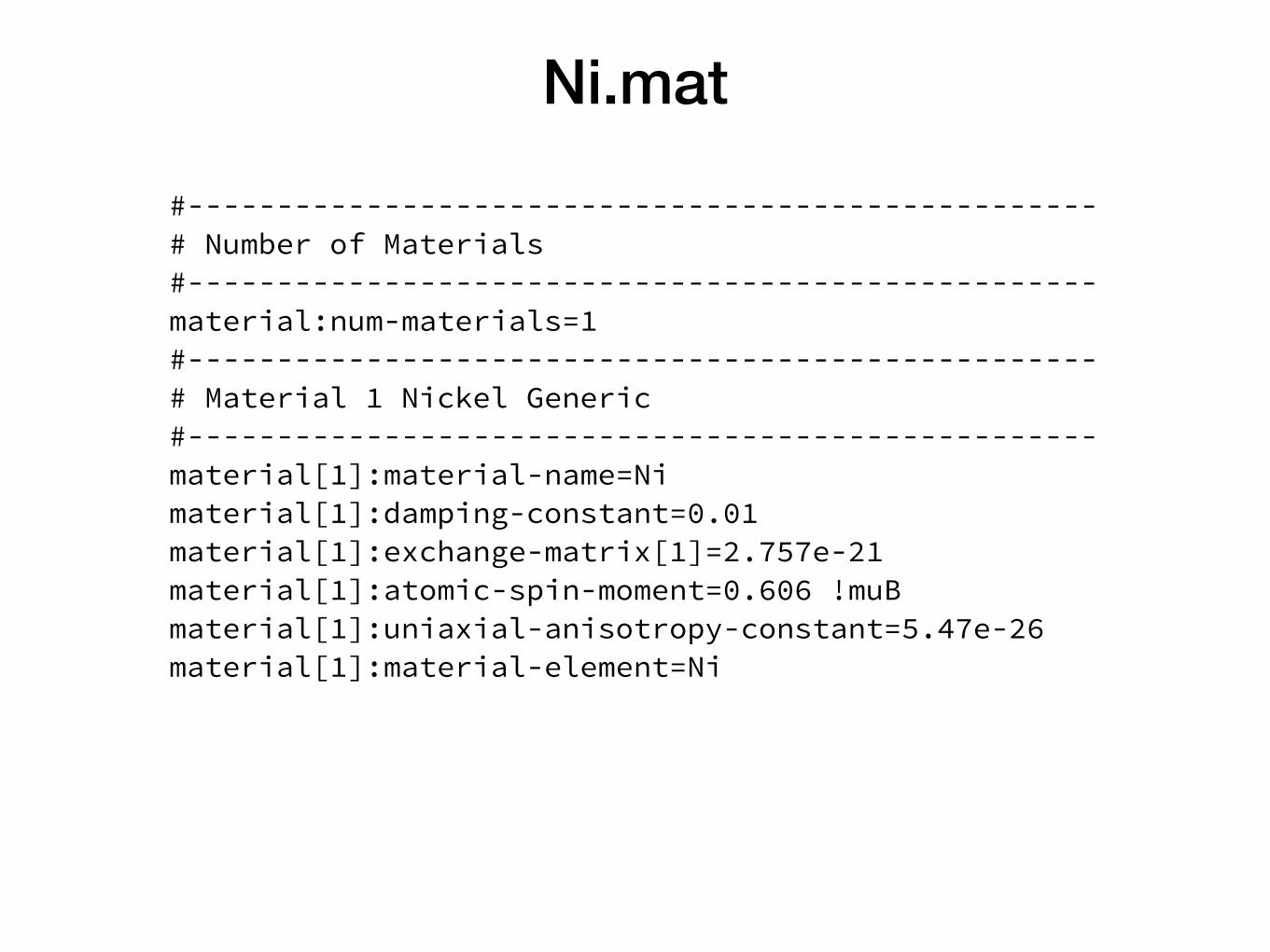
Ni.mat

#--------------------------------------------------- # Number of Materials #--------------------------------------------------- material:num-materials=1 #--------------------------------------------------- # Material 1 Nickel Generic #--------------------------------------------------- material[1]:material-name=Ni material[1]:damping-constant=0.01 material[1]:exchange-matrix[1]=2.757e-21 material[1]:atomic-spin-moment=0.606 !muB material[1]:uniaxial-anisotropy-constant=5.47e-26 material[1]:material-element=Ni

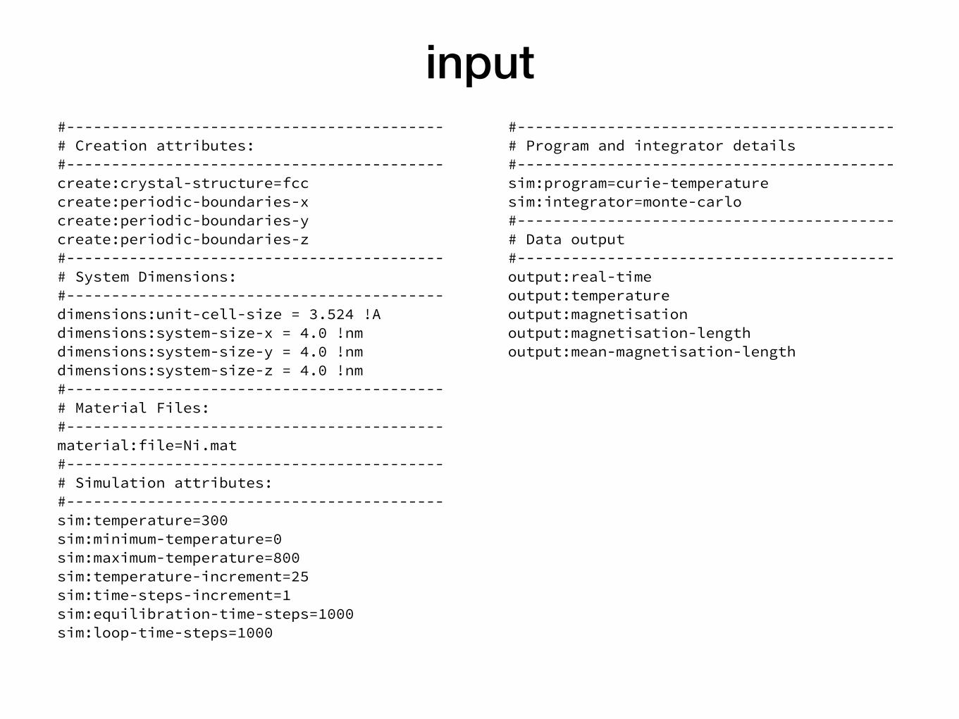
input#------------------------------------------ # Creation attributes: #------------------------------------------ create:crystal-structure=fcc create:periodic-boundaries-x create:periodic-boundaries-y create:periodic-boundaries-z #------------------------------------------ # System Dimensions: #------------------------------------------ dimensions:unit-cell-size = 3.524 !A dimensions:system-size-x = 4.0 !nm dimensions:system-size-y = 4.0 !nm dimensions:system-size-z = 4.0 !nm #------------------------------------------ # Material Files: #------------------------------------------ material:file=Ni.mat #------------------------------------------ # Simulation attributes: #------------------------------------------ sim:temperature=300 sim:minimum-temperature=0 sim:maximum-temperature=800 sim:temperature-increment=25 sim:time-steps-increment=1 sim:equilibration-time-steps=1000 sim:loop-time-steps=1000

#------------------------------------------ # Program and integrator details #------------------------------------------ sim:program=curie-temperature sim:integrator=monte-carlo #------------------------------------------ # Data output #------------------------------------------ output:real-time output:temperature output:magnetisation output:magnetisation-length output:mean-magnetisation-length

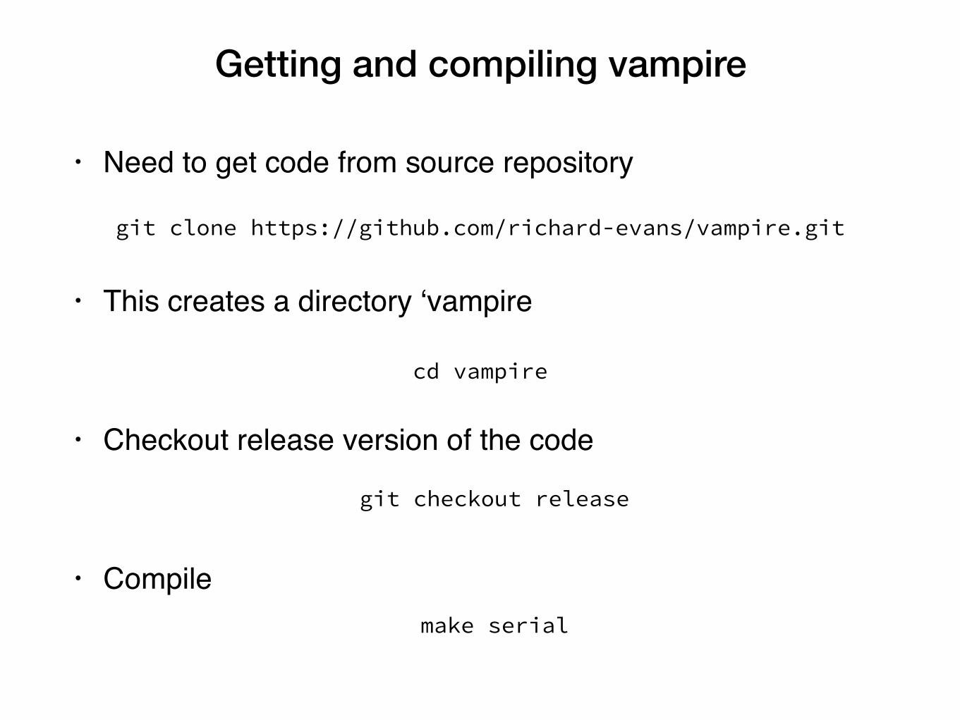
Getting and compiling vampire

• Need to get code from source repository

• This creates a directory ‘vampire

• Checkout release version of the code

• Compile

git clone https://github.com/richard-evans/vampire.git

git checkout release

make serial

cd vampire

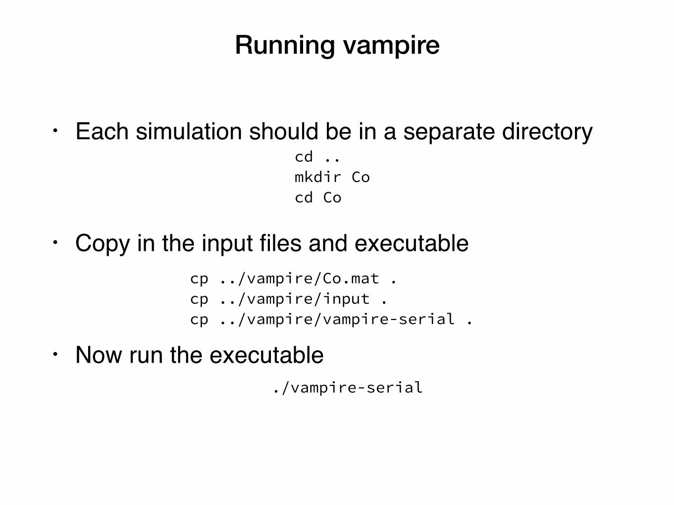
Running vampire

• Each simulation should be in a separate directory

• Copy in the input files and executable

• Now run the executable

cd .. mkdir Co cd Co

./vampire-serial

cp ../vampire/Co.mat . cp ../vampire/input . cp ../vampire/vampire-serial .

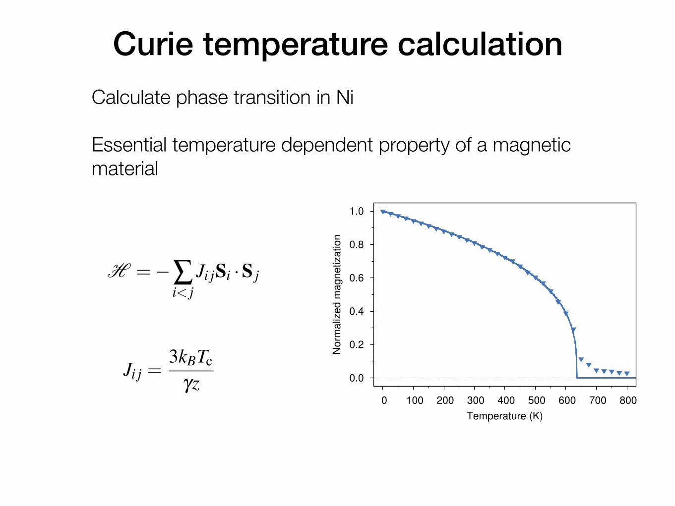
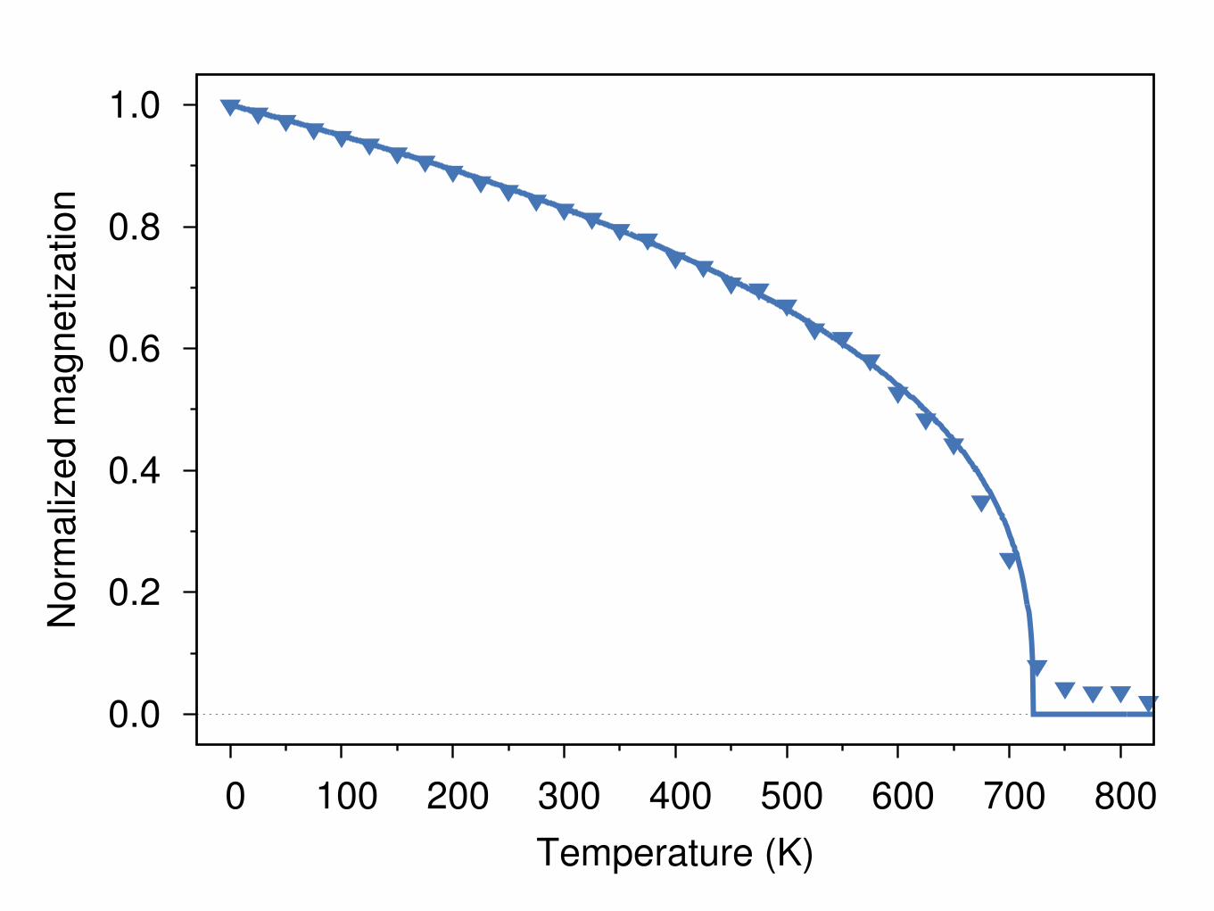
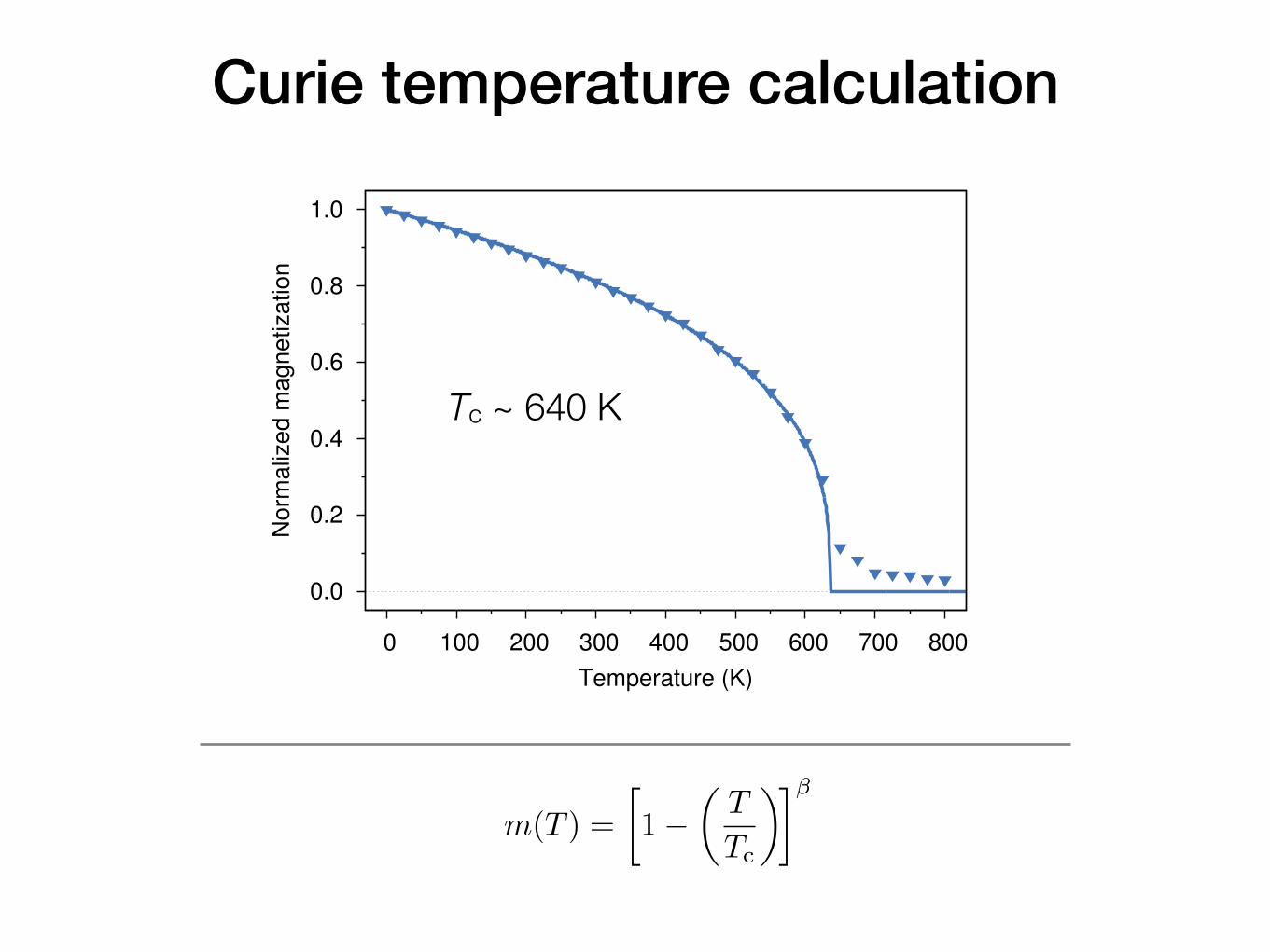
Curie temperature calculationCalculate phase transition in Ni

Essential temperature dependent property of a magnetic material

0.0

0.2

0.4

0.6

0.8

1.0

0 100 200 300 400 500 600 700 800

Norm

aliz

ed m

agnetiz

atio

n

Temperature (K)

2

sults. For a recent extensive comparison between classical andquantum Heisenberg Hamiltonians see (? ). For the classicalstatistics

mc(T ) = 1− kBTJ0

1N ∑

kkk

11− γkkk

≈ 1− 13

TTc, (1)

where T is the temperature, kB is the Boltzmann constant andTc is the Curie temperature and we have used the RPA relationto relate W and Tc (J0/3 ≈ WkBTc)? (exact for the sphericalmodel? ), where W = (1/N ∑kkk

11−γkkk

) is the Watson integral.Under the same conditions in the quantum Heisenberg case

one obtains the T 3/2 Bloch law,

mq(T ) = 1− 13

s!

TTc

"3/2(2)

where s is a slope factor and defined as

s = S1/2 (2πW )−3/2 ζ (3/2). (3)

where S is the spin value and ζ (x) the well-known Riemannζ function, and RPA relation (3kBTc = J0S2/W ) has beenused. We note that Kuz’min22 utilized semi-classical linearspin wave theory to determine s, and so use the experimen-tally measured magnetic moment of the studied metals.

Mapping between the classical and quantum m(T ) expres-sions is done simply by equalizing Eqs. (1) and (2) yield-ing τcl = sτ3/2

q . This expression therefore relates the ther-mal fluctuations between the classical and quantum Heisen-berg models at low temperatures. At higher temperaturesmore terms are required to describe m(T ) for both approaches,making the simple identification between temperatures cum-bersome. At temperatures close to and above Tc, βεkkk → 0is a small parameter and thus the thermal Bose distribu-tion 1/(exp(βεkkk)− 1) ≈ βεkkk tends to the Boltzmann distri-bution, thus the effect of the spin quantization is negligiblehere. For this temperature region, a power law is expected,m(τ)≈ (1− τ)β , where β = 1/3 for the Heisenberg model inboth cases.

The existence of a simple relation between classical andquantum temperature dependent magnetization at low temper-atures leads to the question - does a similar scaling quantita-tively describe the behavior of elemental ferromagnets for thewhole range of temperatures? Our starting point is to repre-sent the temperature dependent magnetization in the simplestform arising from a straightforward interpolation of the Blochlaw and critical behavior24 given by the Curie-Bloch equation

m(τ) = (1− τα)β (4)

where α is an empirical constant and β ≈ 1/3 is the criticalexponent. We will demonstrate that this simple expression issufficient to describe the temperature dependent magnetiza-tion in elemental ferromagnets with a single fitting parameterα .

An alternative to the Curie-Bloch equation was proposedby Kuz’min22 which has the form

m(τ) = [1− sτ3/2 − (1− s)τ p]1/3. (5)

The parameters s and p are taken as fitting parameters, whereit was found that p = 5/2 for all ferromagnets except for Feand s relates to the shape of the m(T ) curve and correspondsto the extent that the magnetization follows Bloch’s law at lowtemperatures. In the case of a pure Bloch ferromagnet wherep = 3/2 and α = p equations (4) and (5) are identical, demon-strating the same physical origin of these phenomenologicalequations. At low temperatures these functions are related byτα = sτ3/2 which can be used to estimate α from s?

While Kuz’min’s equation quantitatively describes theshape of the magnetization curve, it does not link the macro-scopic Curie temperature to microscopic exchange interac-tions. These exchange interactions can be conveniently de-termined by ab-initio first principles calculations? . Exchangeinteractions calculated from first principles are often longranged and oscillatory in nature and so analytical determi-nation of the Curie temperature can be done with a numberof different standard approaches such as mean-field (MFA)or random phase approximations (RPA), neither of which areparticularly accurate due to the approximations involved. Amuch more successful method is incorporating the micro-scopic exchange interactions into a multiscale atomistic spinmodel which has been shown to yield Curie temperaturesmuch closer to experiment21. The clear advantage of this ap-proach is the direct linking of electronic scale calculated pa-rameters to macroscopic thermodynamic magnetic propertiessuch as the Curie temperature. What is interesting is that theclassical spin fluctuations give the correct Tc for a wide rangeof magnetic materials21? , suggesting that the particular valueof the exchange parameters and the shape of the m(T ) curveare largely independent quantities, as suggested by Eq. (3).The difficulty with the classical model is that the shape of thecurve is intrinsically wrong when compared to experiment.

To obtain accurate data for the classical temperature depen-dent magnetization for the elemental ferromagnets Co, Fe, Niand Gd we proceed to simulate them using the classical atom-istic spin model. The energetics of the system are describedby the classical spin Hamiltonian15 of the form

H =−∑i< j

Ji jSi ·S j (6)

where Si and S j are unit vectors describing the direction of thelocal and nearest neighbor magnetic moments at each atomicsite and Ji j is the nearest neighbor exchange energy given by?

Ji j =3kBTc

γz(7)

where γ(W ) gives a correction factor from the MFA and whichfor RPA γ = 1/W . The numerical calculations have been car-ried out using the VAMPIRE software package25. The sim-ulated system for Co, Ni, Fe and Gd consists of a cube 20nm3 in size with periodic boundary conditions applied to re-move any surface effects. The equilibrium temperature depen-dent properties of the system are calculated using the Hinzke-Nowak Monte Carlo algorithm15,26 resulting in the calculatedtemperature dependent magnetization curves for each elementshown in Fig. 1.

2

sults. For a recent extensive comparison between classical andquantum Heisenberg Hamiltonians see (? ). For the classicalstatistics

mc(T ) = 1− kBTJ0

1N ∑

kkk

11− γkkk

≈ 1− 13

TTc, (1)

where T is the temperature, kB is the Boltzmann constant andTc is the Curie temperature and we have used the RPA relationto relate W and Tc (J0/3 ≈ WkBTc)? (exact for the sphericalmodel? ), where W = (1/N ∑kkk

11−γkkk

) is the Watson integral.Under the same conditions in the quantum Heisenberg case

one obtains the T 3/2 Bloch law,

mq(T ) = 1− 13

s!

TTc

"3/2(2)

where s is a slope factor and defined as

s = S1/2 (2πW )−3/2 ζ (3/2). (3)

where S is the spin value and ζ (x) the well-known Riemannζ function, and RPA relation (3kBTc = J0S2/W ) has beenused. We note that Kuz’min22 utilized semi-classical linearspin wave theory to determine s, and so use the experimen-tally measured magnetic moment of the studied metals.

Mapping between the classical and quantum m(T ) expres-sions is done simply by equalizing Eqs. (1) and (2) yield-ing τcl = sτ3/2

q . This expression therefore relates the ther-mal fluctuations between the classical and quantum Heisen-berg models at low temperatures. At higher temperaturesmore terms are required to describe m(T ) for both approaches,making the simple identification between temperatures cum-bersome. At temperatures close to and above Tc, βεkkk → 0is a small parameter and thus the thermal Bose distribu-tion 1/(exp(βεkkk)− 1) ≈ βεkkk tends to the Boltzmann distri-bution, thus the effect of the spin quantization is negligiblehere. For this temperature region, a power law is expected,m(τ)≈ (1− τ)β , where β = 1/3 for the Heisenberg model inboth cases.

The existence of a simple relation between classical andquantum temperature dependent magnetization at low temper-atures leads to the question - does a similar scaling quantita-tively describe the behavior of elemental ferromagnets for thewhole range of temperatures? Our starting point is to repre-sent the temperature dependent magnetization in the simplestform arising from a straightforward interpolation of the Blochlaw and critical behavior24 given by the Curie-Bloch equation

m(τ) = (1− τα)β (4)

where α is an empirical constant and β ≈ 1/3 is the criticalexponent. We will demonstrate that this simple expression issufficient to describe the temperature dependent magnetiza-tion in elemental ferromagnets with a single fitting parameterα .

An alternative to the Curie-Bloch equation was proposedby Kuz’min22 which has the form

m(τ) = [1− sτ3/2 − (1− s)τ p]1/3. (5)

The parameters s and p are taken as fitting parameters, whereit was found that p = 5/2 for all ferromagnets except for Feand s relates to the shape of the m(T ) curve and correspondsto the extent that the magnetization follows Bloch’s law at lowtemperatures. In the case of a pure Bloch ferromagnet wherep = 3/2 and α = p equations (4) and (5) are identical, demon-strating the same physical origin of these phenomenologicalequations. At low temperatures these functions are related byτα = sτ3/2 which can be used to estimate α from s?

While Kuz’min’s equation quantitatively describes theshape of the magnetization curve, it does not link the macro-scopic Curie temperature to microscopic exchange interac-tions. These exchange interactions can be conveniently de-termined by ab-initio first principles calculations? . Exchangeinteractions calculated from first principles are often longranged and oscillatory in nature and so analytical determi-nation of the Curie temperature can be done with a numberof different standard approaches such as mean-field (MFA)or random phase approximations (RPA), neither of which areparticularly accurate due to the approximations involved. Amuch more successful method is incorporating the micro-scopic exchange interactions into a multiscale atomistic spinmodel which has been shown to yield Curie temperaturesmuch closer to experiment21. The clear advantage of this ap-proach is the direct linking of electronic scale calculated pa-rameters to macroscopic thermodynamic magnetic propertiessuch as the Curie temperature. What is interesting is that theclassical spin fluctuations give the correct Tc for a wide rangeof magnetic materials21? , suggesting that the particular valueof the exchange parameters and the shape of the m(T ) curveare largely independent quantities, as suggested by Eq. (3).The difficulty with the classical model is that the shape of thecurve is intrinsically wrong when compared to experiment.

To obtain accurate data for the classical temperature depen-dent magnetization for the elemental ferromagnets Co, Fe, Niand Gd we proceed to simulate them using the classical atom-istic spin model. The energetics of the system are describedby the classical spin Hamiltonian15 of the form

H =−∑i< j

Ji jSi ·S j (6)

where Si and S j are unit vectors describing the direction of thelocal and nearest neighbor magnetic moments at each atomicsite and Ji j is the nearest neighbor exchange energy given by?

Ji j =3kBTc

γz(7)

where γ(W ) gives a correction factor from the MFA and whichfor RPA γ = 1/W . The numerical calculations have been car-ried out using the VAMPIRE software package25. The sim-ulated system for Co, Ni, Fe and Gd consists of a cube 20nm3 in size with periodic boundary conditions applied to re-move any surface effects. The equilibrium temperature depen-dent properties of the system are calculated using the Hinzke-Nowak Monte Carlo algorithm15,26 resulting in the calculatedtemperature dependent magnetization curves for each elementshown in Fig. 1.

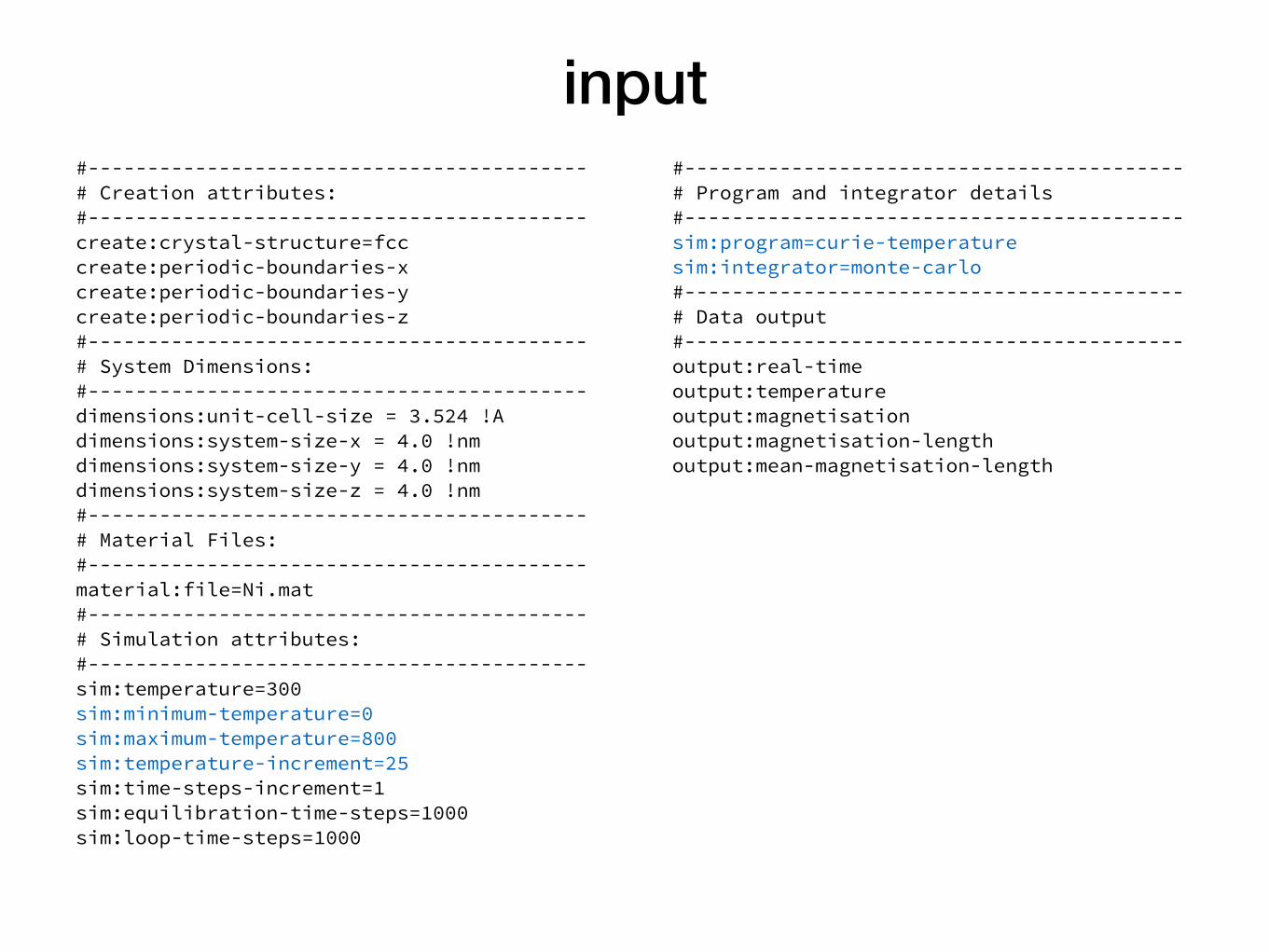
input#------------------------------------------ # Creation attributes: #------------------------------------------ create:crystal-structure=fcc create:periodic-boundaries-x create:periodic-boundaries-y create:periodic-boundaries-z #------------------------------------------ # System Dimensions: #------------------------------------------ dimensions:unit-cell-size = 3.524 !A dimensions:system-size-x = 4.0 !nm dimensions:system-size-y = 4.0 !nm dimensions:system-size-z = 4.0 !nm #------------------------------------------ # Material Files: #------------------------------------------ material:file=Ni.mat #------------------------------------------ # Simulation attributes: #------------------------------------------ sim:temperature=300 sim:minimum-temperature=0 sim:maximum-temperature=800 sim:temperature-increment=25 sim:time-steps-increment=1 sim:equilibration-time-steps=1000 sim:loop-time-steps=1000

#------------------------------------------ # Program and integrator details #------------------------------------------ sim:program=curie-temperature sim:integrator=monte-carlo #------------------------------------------ # Data output #------------------------------------------ output:real-time output:temperature output:magnetisation output:magnetisation-length output:mean-magnetisation-length

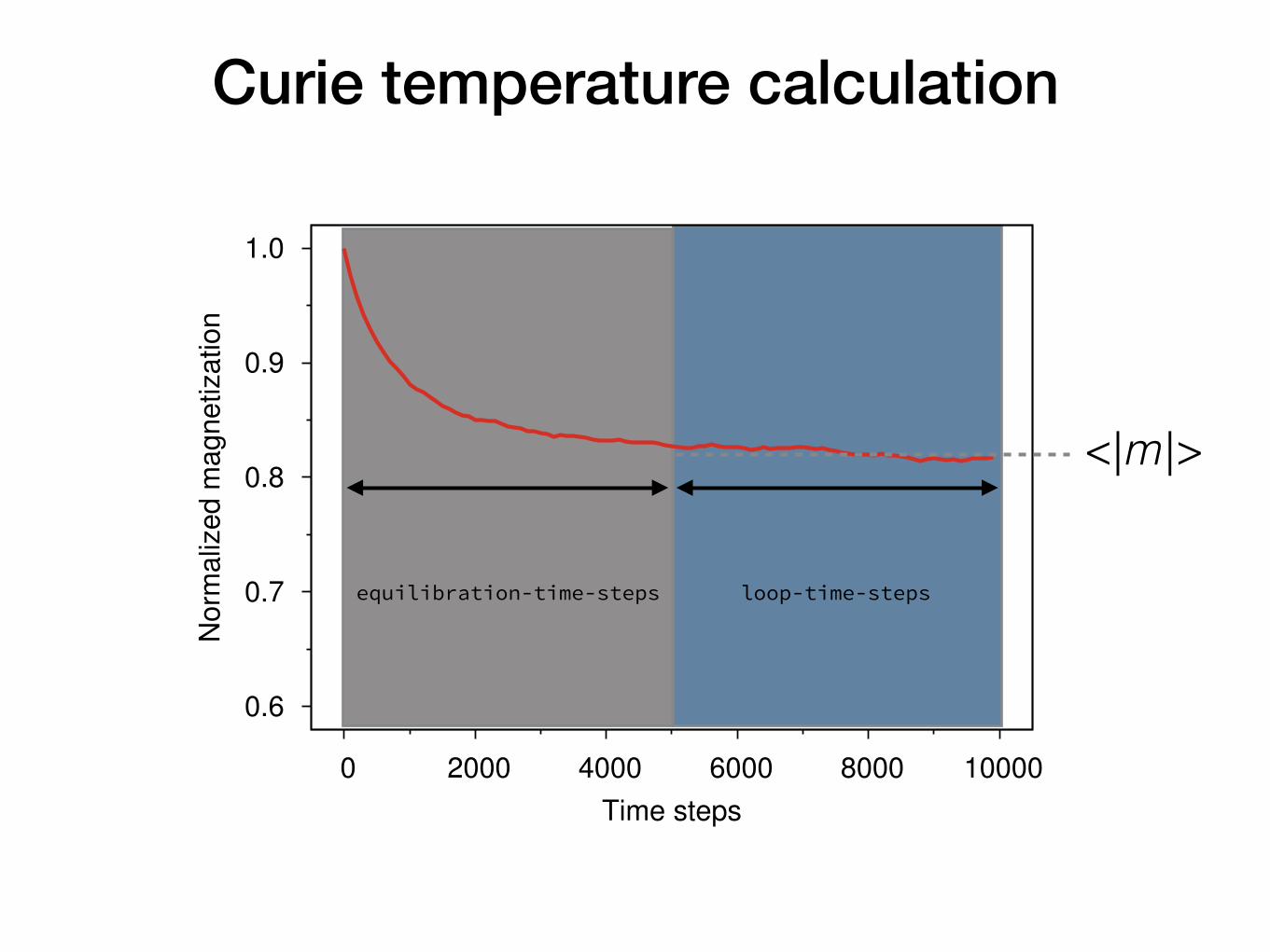
Curie temperature calculation

0.6

0.7

0.8

0.9

1.0

0 2000 4000 6000 8000 10000

Norm

aliz

ed m

agnetiz

atio

n

Time steps

equilibration-time-steps loop-time-steps

<|m |>

0.0

0.2

0.4

0.6

0.8

1.0

0 100 200 300 400 500 600 700 800

Norm

aliz

ed m

agnetiz

atio

n

Temperature (K)

Curie temperature calculation

0.0

0.2

0.4

0.6

0.8

1.0

0 100 200 300 400 500 600 700 800

No

rma

lize

d m

ag

ne

tiza

tion

Temperature (K)

3

the dominant atomic species in Nd2Fe14B, it is expectedthat the magnetization is dominated by the Fe sublattice.

Fe exchange interactions

The first approach in classical spin models is to calcu-late an e↵ective pairwise nearest neighbor exchange inter-action, derived from the Curie temperature of the systemusing a molecular field approximation. For Nd2Fe14B thisapproach is complicated by the complex crystal struc-ture which makes a global nearest neighbor distance is apoorly defined quantity, leading to di↵erent numbers ofinteractions for di↵erent atomic sites. As a first approxi-mation we therefore utilize the results of ab-initio calcu-lations of exchange interactions in bcc Fe7. The rangedependence of the calculated exchange interactions con-veniently fit to an exponential function for the first fivecoordination shells, and so the fitted function gives JFe(r)is given by

JFe(r) = J0 + Jr exp(�r/r0) (7)

where r is the interatomic separation, r0 is a characteris-tic distance, and J0 and Jr are fitting constants. The ex-change interactions are truncated to zero for interatomicseparations greater than 5A. The fitted function is shownin Fig. 2. Applying the fitted exchange interactions to theNd2Fe14B system yields a simulated Curie temperatureof around 800K. Already the greater interatomic sepa-ration reduces the Curie temperature compared to bulkbcc Fe, but this value is still higher than the experimen-tal value of 585K. Given the significantly lower densityof the Fe sublattice compared with bcc Fe, it is not un-reasonable to expect reduced overlap of atomic orbitalsof the Fe sites, with a corresponding reduction in the ex-change interactions. To approximate this e↵ect we treatthe reduction in the pairwise exchange interactions bystraightforward scaling of the ab-initio values so that thecalculated Curie temperature agrees better with experi-ment. The scaled curve and values are shown in Fig. 2,and the values used for the scaled fitted function are pre-sented in Tab. I. This crude scaling is not particularlysatisfactory, but has the advantage of at least maintain-ing the long range nature and distance dependence ofthe exchange interactions and is at least as good as thenearest neighbor approximation commonly employed.

Nd exchange interactions

The Nd sublattice is known to couple ferromagneticallyto the Fe sublattice at higher temperatures, and experi-mental measurements8 show a high degree of ordering ofthe Nd sublattice at room temperature. This orderingat significant fractions of the Curie temperature necessi-tates a relatively strong exchange coupling between theFe and Nd sites, at least compared with bulk Nd. In con-trast crystal field calculations suggest a weak exchange

−0.5

0.0

0.5

1.0

1.5

2.0

2.5

3.0

3.5

2 2.5 3 3.5 4 4.5 5

Exc

hang

e en

ergy

(× 1

0−21 J

)

Interatomic spacing (Å)

ab−initio dataFitted function

Scaled data

FIG. 2. Range dependence of the exchange interactions fromab-initio calculations7. Scaled data arising from reduced over-lap of atomic orbitals is used to calculate the Fe-Fe interac-tions in the Nd crystal. Color Online.

coupling9 and so the strength of the Nd-Fe exchange in-teraction is an open question. We therefore treat theFe-Nd exchange is a variable parameter in the model inorder to best fit the available experimental data. Thenearest neighbor distance is better defined for the Fe-Nd interactions, and so a cut o↵ distance of 4Ais chosenin the nearest neighbor approach, where all interactionshave the same strength. The Nd-Nd interactions are as-sumed to be negligible, and are consequently ignored inthe model.

Temperature dependent magnetization

Using the derived exchange parameters described pre-viously, we now present atomistic calculations of the tem-perature dependent magnetization of the Fe sublatticeusing the Monte Carlo method and shown in Fig. 3(a).By empirical interpolation of the Bloch law and criticalbehavior10, the reduced temperature dependent magne-tization is given by the expression:

m(T ) =

1�

✓T

Tc

◆↵��(8)

where T is the temperature, Tc is the Curie tempera-ture, ↵ is an empirical constant and � is the critical ex-ponent. Since classical systems do not follow Bloch’sLaw (low temperatures always have finite fluctuations inm), ↵ = 1, and so fitting to the calculated tempera-ture dependent magnetization yields a critical exponentof � = 0.343 ± 0.002 and Curie temperature of 581 K.Due to the long range nature of the exchange interac-tions, the critical exponent � is slightly lower than the3D Heisenberg model, also seen in calculations of FePt11.Due to the neglect of quantum e↵ects within the clas-

sical spin model, the calculated temperature dependent

3

the dominant atomic species in Nd2Fe14B, it is expectedthat the magnetization is dominated by the Fe sublattice.

Fe exchange interactions

The first approach in classical spin models is to calcu-late an e↵ective pairwise nearest neighbor exchange inter-action, derived from the Curie temperature of the systemusing a molecular field approximation. For Nd2Fe14B thisapproach is complicated by the complex crystal struc-ture which makes a global nearest neighbor distance is apoorly defined quantity, leading to di↵erent numbers ofinteractions for di↵erent atomic sites. As a first approxi-mation we therefore utilize the results of ab-initio calcu-lations of exchange interactions in bcc Fe7. The rangedependence of the calculated exchange interactions con-veniently fit to an exponential function for the first fivecoordination shells, and so the fitted function gives JFe(r)is given by

JFe(r) = J0 + Jr exp(�r/r0) (7)

where r is the interatomic separation, r0 is a characteris-tic distance, and J0 and Jr are fitting constants. The ex-change interactions are truncated to zero for interatomicseparations greater than 5A. The fitted function is shownin Fig. 2. Applying the fitted exchange interactions to theNd2Fe14B system yields a simulated Curie temperatureof around 800K. Already the greater interatomic sepa-ration reduces the Curie temperature compared to bulkbcc Fe, but this value is still higher than the experimen-tal value of 585K. Given the significantly lower densityof the Fe sublattice compared with bcc Fe, it is not un-reasonable to expect reduced overlap of atomic orbitalsof the Fe sites, with a corresponding reduction in the ex-change interactions. To approximate this e↵ect we treatthe reduction in the pairwise exchange interactions bystraightforward scaling of the ab-initio values so that thecalculated Curie temperature agrees better with experi-ment. The scaled curve and values are shown in Fig. 2,and the values used for the scaled fitted function are pre-sented in Tab. I. This crude scaling is not particularlysatisfactory, but has the advantage of at least maintain-ing the long range nature and distance dependence ofthe exchange interactions and is at least as good as thenearest neighbor approximation commonly employed.

Nd exchange interactions

The Nd sublattice is known to couple ferromagneticallyto the Fe sublattice at higher temperatures, and experi-mental measurements8 show a high degree of ordering ofthe Nd sublattice at room temperature. This orderingat significant fractions of the Curie temperature necessi-tates a relatively strong exchange coupling between theFe and Nd sites, at least compared with bulk Nd. In con-trast crystal field calculations suggest a weak exchange

−0.5

0.0

0.5

1.0

1.5

2.0

2.5

3.0

3.5

2 2.5 3 3.5 4 4.5 5

Exc

hang

e en

ergy

(× 1

0−21 J

)

Interatomic spacing (Å)

ab−initio dataFitted function

Scaled data

FIG. 2. Range dependence of the exchange interactions fromab-initio calculations7. Scaled data arising from reduced over-lap of atomic orbitals is used to calculate the Fe-Fe interac-tions in the Nd crystal. Color Online.

coupling9 and so the strength of the Nd-Fe exchange in-teraction is an open question. We therefore treat theFe-Nd exchange is a variable parameter in the model inorder to best fit the available experimental data. Thenearest neighbor distance is better defined for the Fe-Nd interactions, and so a cut o↵ distance of 4Ais chosenin the nearest neighbor approach, where all interactionshave the same strength. The Nd-Nd interactions are as-sumed to be negligible, and are consequently ignored inthe model.

Temperature dependent magnetization

Using the derived exchange parameters described pre-viously, we now present atomistic calculations of the tem-perature dependent magnetization of the Fe sublatticeusing the Monte Carlo method and shown in Fig. 3(a).By empirical interpolation of the Bloch law and criticalbehavior10, the reduced temperature dependent magne-tization is given by the expression:

m(T ) =

1�

✓T

Tc

◆↵��(8)

where T is the temperature, Tc is the Curie tempera-ture, ↵ is an empirical constant and � is the critical ex-ponent. Since classical systems do not follow Bloch’sLaw (low temperatures always have finite fluctuations inm), ↵ = 1, and so fitting to the calculated tempera-ture dependent magnetization yields a critical exponentof � = 0.343 ± 0.002 and Curie temperature of 581 K.Due to the long range nature of the exchange interac-tions, the critical exponent � is slightly lower than the3D Heisenberg model, also seen in calculations of FePt11.Due to the neglect of quantum e↵ects within the clas-

sical spin model, the calculated temperature dependent

Tc ~ 640 K

Gnuplot for plotting data and curve fitting

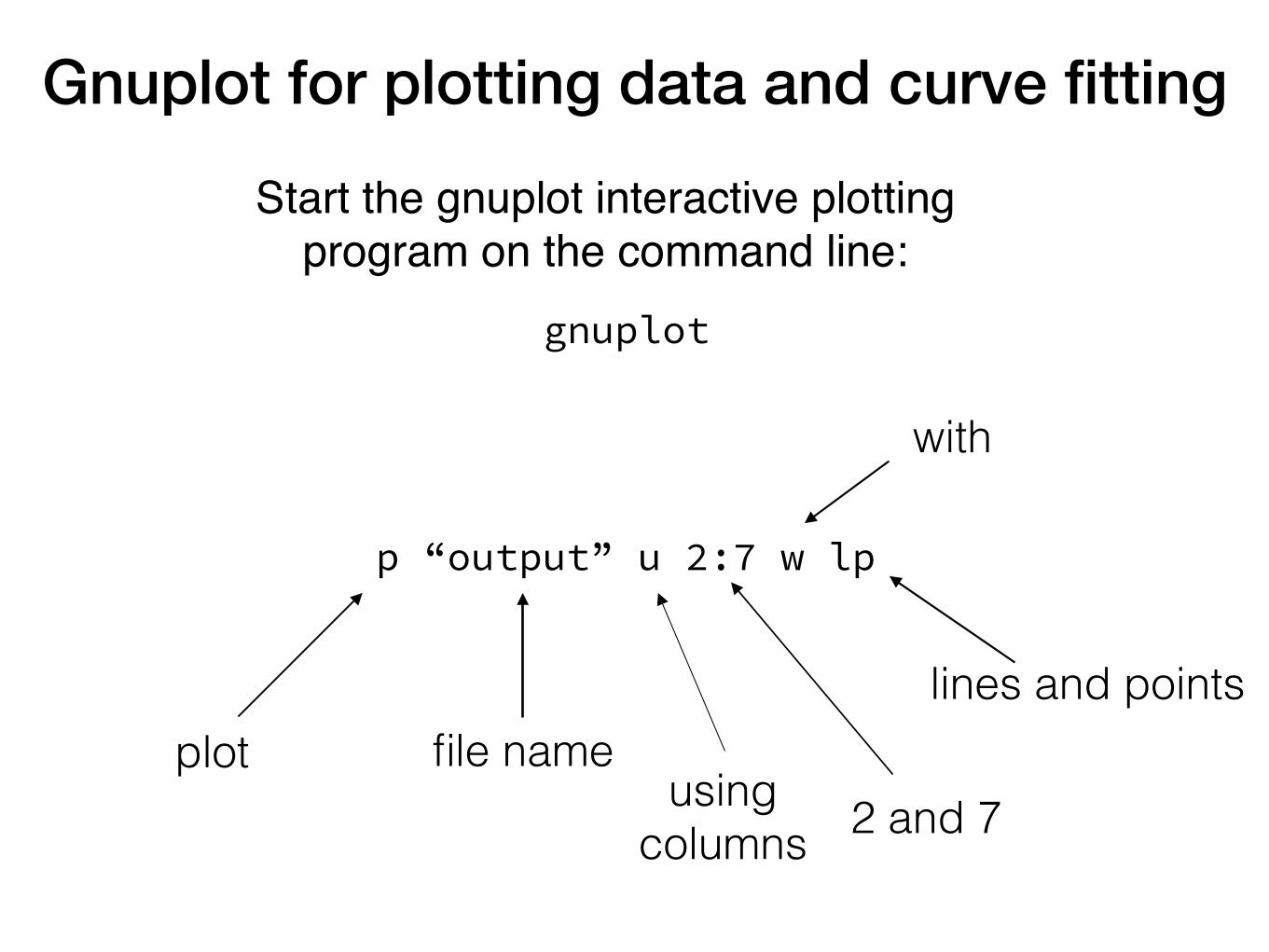
p “output” u 2:7 w lp

plot file nameusing

columns 2 and 7

with

lines and points

Start the gnuplot interactive plotting program on the command line:

gnuplot

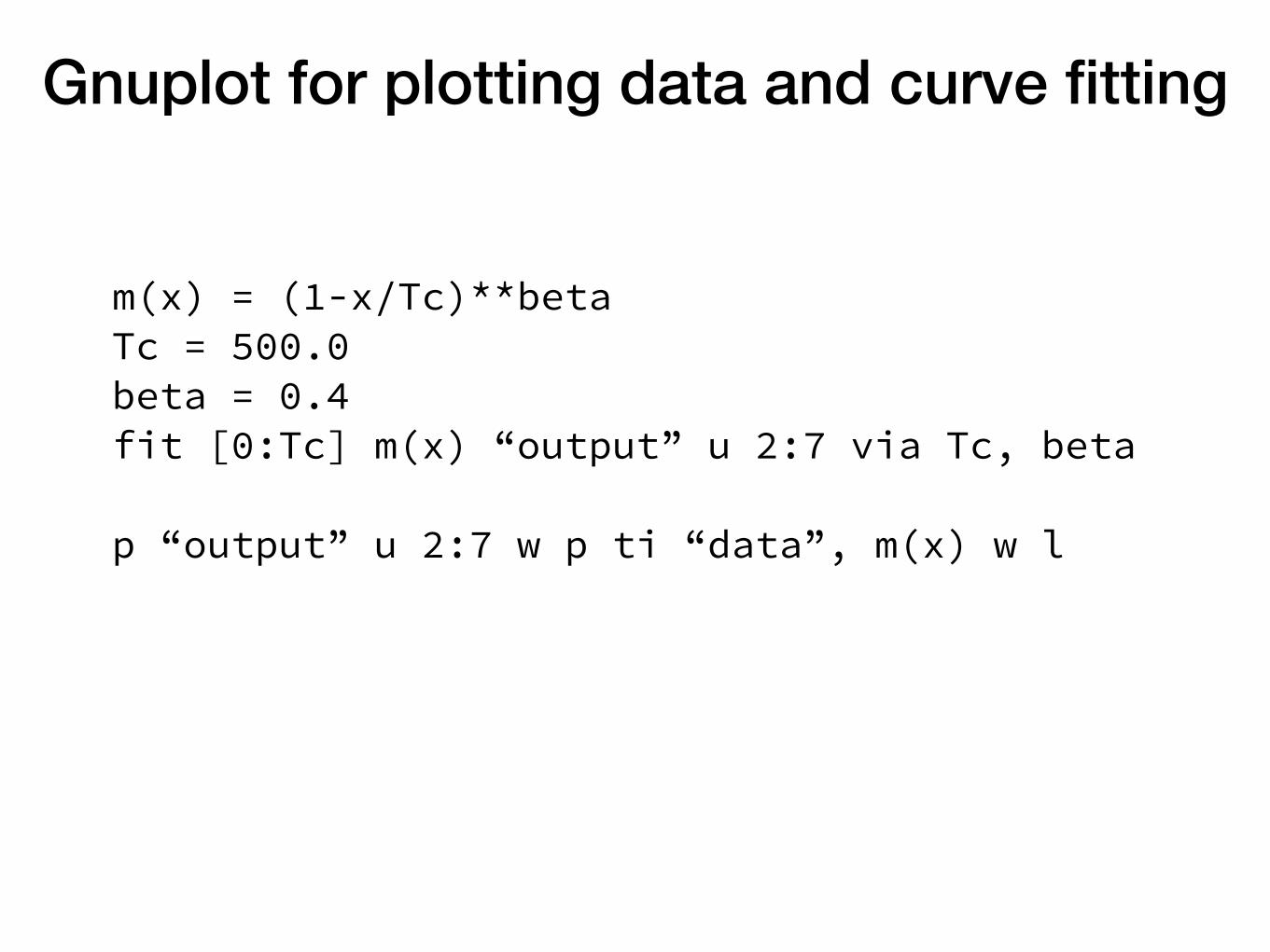
Gnuplot for plotting data and curve fitting

m(x) = (1-x/Tc)**beta Tc = 500.0 beta = 0.4 fit [0:Tc] m(x) “output” u 2:7 via Tc, beta

p “output” u 2:7 w p ti “data”, m(x) w l

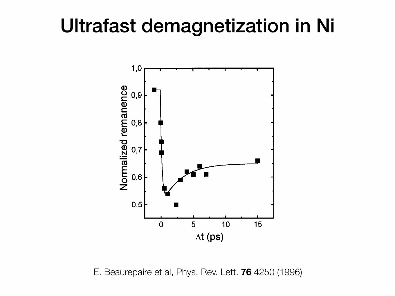
Ultrafast demagnetization in Ni

E. Beaurepaire et al, Phys. Rev. Lett. 76 4250 (1996)

VOLUME 76, NUMBER 22 P HY S I CA L REV I EW LE T T ER S 27 MAY 1996

FIG. 1. (a) Experimental pump-probe setup allowing dynamiclongitudinal Kerr effect and transient transmissivity or reflectiv-ity measurements. (b) Typical Kerr loops obtained on a 22 nmthick Ni sample in the absence of pump beam and for a delayDt ≠ 2.3 ps between the pump and probe pulses. The pumpfluence is 7 mJ cm22. (c) Transient transmissivity [same exper-imental condition as (b)].

transient transmission curve DTyT is displayed inFig. 1(c). For both techniques, we used 60 fs pulsescoming from a 620 nm colliding pulse mode locked dyelaser and amplified by a 5 kHz copper vapor laser. Thetemporal delays between pump and probe are achievedusing a modified Michelson interferometer. The signalsare recorded using a boxcar and a lock-in synchronousdetection. In the case of differential transmission mea-surements, the synchronization is made by chopping thepump beam, while for the MOKE measurements it isdone on the probe beam.The information about the spin dynamics is contained in

the time evolution of the hysteresis loops recorded for eachtime delay Dt. Typical loops obtained for Dt ≠ 2.3 psand in the absence of the pump beam are presented inFig. 1(b). Each hysteresis loop is recorded at a fixed delayby slowly sweeping the magnetic field H. For each H

value, the MOKE signal is averaged over about 100 pulses.The most striking feature is an important decrease of theremanence (signal at zero field) Mr when the pump ison. The complete dynamics MrsDtd for a laser fluenceof 7 mJ cm22 is displayed in Fig. 2. The overall behavioris an important and rapid decrease of Mr which occurswithin 2 ps, followed by a relaxation to a long livedplateau. This figure clearly shows that the magnetizationof the film drops during the first picosecond, indicating afast increase of the spin temperature. It can be noticedthat for negative delays Mr does not completely recoverits value measured in the absence of pump beam. Thispermanent effect is not due to a sample damage as checkedby recording hysteresis loops without the pump beam afterthe dynamical measurements. Possible explanations forthis small permanent change are either heat accumulationor slow motion of the domain walls induced by thepump beam.In order to determine the temperature dynamics, we

analyze Fig. 2 using the static temperature dependenceof the magnetization found in text books. This analysisrelies on a correspondence between the variations of the

FIG. 2. Transient remanent longitudinal MOKE signal of aNi(20 nm)/MgF2(100 nm) film for 7 mJ cm22 pump fluence.The signal is normalized to the signal measured in the absenceof pump beam. The line is a guide to the eye.

spontaneous and remanent magnetization, as is usuallydone in thin film magnetism. This leads to the timevariation of Ts in Fig. 3(a) (dotted points). Regarding thedetermination of the electronic temperature, we assumethat it is proportional to the differential transmittanceshown in Fig. 1(c) as expected for weak DTyT signals.Let us emphasize that this procedure is valid only whena thermalized electron population can be defined. Sincethis effect was never discussed for the case of d electronsin metals, it deserves some comments. As discussed byvarious authors [4–6], the optical pulse creates in themetal film a nascent (nonthermal) electronic distributionthat relaxes due to electron-electron interactions, leadingto a fast increase of the electron temperature. This processcan be described in the random phase approximation(RPA) defining nonthermal and thermal (in the senseof the Fermi-Dirac statistics) electron populations. Thenonthermal electron population is therefore created duringthe pump pulse and disappears with a characteristic timetth (¯500 fs for Au), whereas the temperature of thethermal population increases in the same time scale. Thecontribution of the nonthermal electronic distribution tothe transient optical data is therefore expected to presenta sharp peak around zero probe delay (with a rise timegiven by the temporal resolution) and the thermal electroncontribution should present a delayed extremum aroundtth [5]. A detailed analysis of the transient effects in Nifor short delays is beyond the scope of the present paperand will be presented in a future publication. Let us onlymention that with the present experimental conditionsthe transient reflectivity of the Ni film presents a singlecontribution which is extremum for Dt ≠ 260 fs showingthat the contribution of nonthermal populations is weakand that the thermalization time is tth ¯ 260 fs. Thisshort thermalization time for Ni as compared to Au is

4251

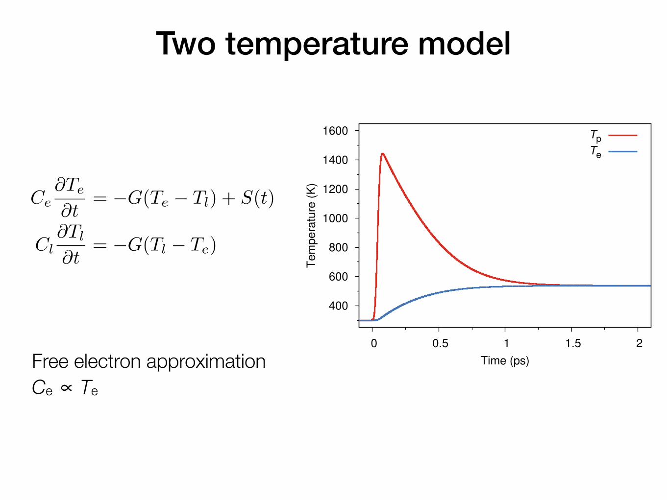
Two temperature model

Free electron approximation Ce ∝ Te

400

600

800

1000

1200

1400

1600

0 0.5 1 1.5 2

Tem

pera

ture

(K

)

Time (ps)

Tp

Te

Ultrafast thermally induced magnetic switching in synthetic ferrimagnets:Supplementary Information

ADDITIONAL MODEL DETAILS

The dynamic properties are modeled using an atom-

istic spin model using the vampire software package[1,

2]. The energetics of the system are described using a

Heisenberg spin Hamiltonian of the form:

Hi,⌫ = HiFe + H

⌫FePt (1)

HiFe = �JFe

X

j

Si · Sj � kFe (Szi )

2

�JFe�FePt

X

µ

Si · Sµ (2)

H⌫FePt = �JFePt

X

µ

S⌫ · Sµ � kFePt (Sz⌫ )

2

�JFe�FePt

X

j

S⌫ · Sj (3)

where JFe is the exchange energy between nearest

neighboring Fe spins, JFePt is the exchange energy be-

tween nearest neighboring FePt spins, JFe�FePt is the ex-

change energy between nearest neighboring Fe and FePt

spins, indices i and j represent local and neighboring Fe

moments and indices ⌫ and µ represent local and neigh-

boring FePt moments respectively, S is a unit vector de-

scribing the direction of the spin moment, and kFe and

kFePt are the uniaxial anisotropy constants for Fe and

FePt atoms respectively. The system is cut from a single

body-centred-cubic crystal in the shape of a cylinder.

The dynamics of each atomic spin is given by the

Landau-Lifshitz-Gilbert equation applied at the atom-

istic level and given by:

@Si

@t= � �

(1 + ↵2i )[Si ⇥H

ie↵ + ↵iSi ⇥ (Si ⇥H

ie↵)] (4)

where � = 1.76 ⇥ 1011

JT�1

s�1

is the gyromagnetic ra-

tio, ↵i is the Gilbert damping parameter for each layer,

and Hie↵ is the net magnetic field. The LLG equation de-

scribes the interaction of an atomic spin moment i withan e↵ective magnetic field, which is obtained from the

negative first derivative of the complete spin Hamilto-

nian and the addition of a Langevin thermal term, such

that the total e↵ective field on each spin is:

Hie↵ = � 1

µs

@H

@Si+H

i,�th . (5)

The thermal field in each spatial dimension � is rep-

resented by a gaussian distribution �(t) with a mean of

zero given by:

Hith = �(t)

s2↵ikBT

�µs�t(6)

where kB is the Boltzmann constant, T is the system

temperature, and �t is the integration time step. The

system is integrated using the Heun numerical scheme

and a timestep of �t = 1.0⇥ 10�16

s.[2]

For the calculations, the system is first equilibrated

for 2 ps at room temperature before the application of a

temperature pulse, which is su�cient to thermalise the

system. The temperature of the spin system is linked

to the electron temperature, leading to a rapid increase

of the temperature inducing ultrafast magnetization dy-

namics. After a few ps the energy is transferred to the

phonon system which leaves the overall system at an el-

evated temperature.

The temporal evolution of the electron temperature is

calculated using the two temperature model[3]:

Ce@Te

@t= �G(Te � Tl) + S(t) (7)

Cl@Tl

@t= �G(Tl � Te) (8)

where Ce and Cl are the electron and lattice hat ca-

pacities, Te is the electron temperature, Tl is the lattice

(phonon) temperature, G is the electron-lattice coupling

factor, and S(t) is a time-dependent Gaussian heat pulse

which adds energy to the electron system representing

the laser pulse. The time evolution of the electron tem-

perature is solved using numerical integration using a

simple Euler scheme. The parameters used in our simu-

lations are representative of a metal, with G = 9⇥1017

W

m�3

K�1

, Ce = 2.25⇥ 102J m

�3K

�1and Cl = 3.1⇥ 10

6

J m�3

K�1

.

DYNAMIC SWITCHING WITH LOWEXCHANGE COUPLING

To test the robustness of the switching in the case of

lower exchange coupling, an additional simulation of the

switching was performed using an interlayer exchange

coupling of 6 mJ/m2, equivalent to�2.235⇥10

�22J/link,

as presented in Fig 1.

While qualitatively similar to the case of strong ex-

change coupling, the switching dynamics are much slower

due to the lower exchange field. However, the exchange

field is su�cient to induce a transient ferromagnetic state

between the sublattices, which drives the switching pro-

cess as the two sublattices mutually precess each other.

As in the strong coupling case, the magnetic anisotropy

of the hard layer is essential to stabilise the reversed state

in the faster layer, ensuring reversal.

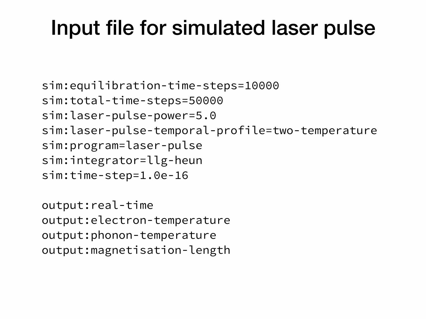
Input file for simulated laser pulse

sim:equilibration-time-steps=10000 sim:total-time-steps=50000 sim:laser-pulse-power=5.0 sim:laser-pulse-temporal-profile=two-temperature sim:program=laser-pulse sim:integrator=llg-heun sim:time-step=1.0e-16

output:real-time output:electron-temperature output:phonon-temperature output:magnetisation-length

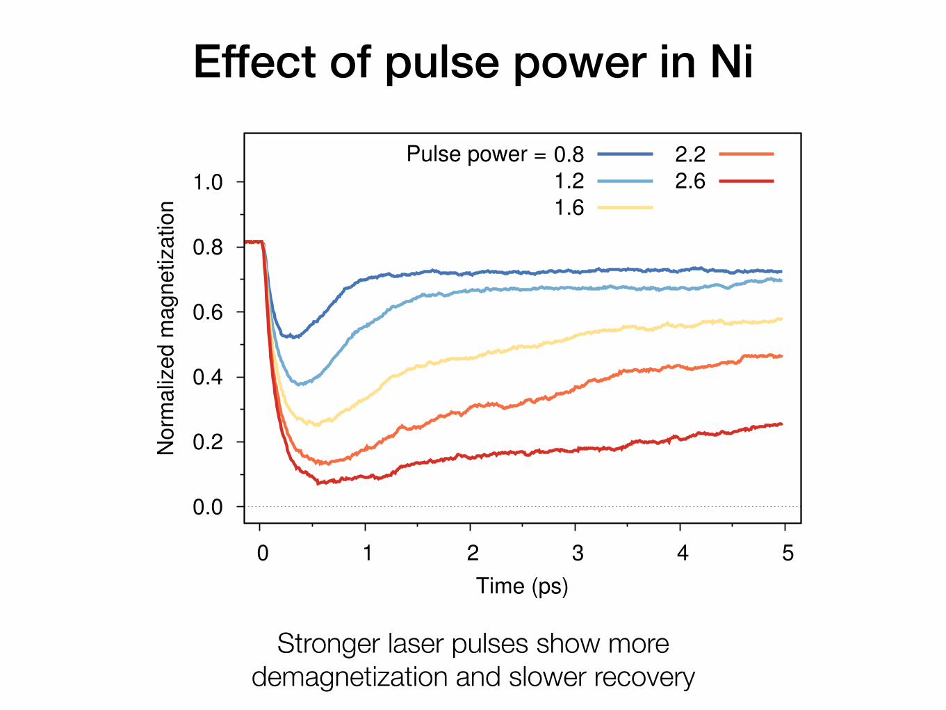
Effect of pulse power in Ni

Stronger laser pulses show more demagnetization and slower recovery

0.0

0.2

0.4

0.6

0.8

1.0

0 1 2 3 4 5

No

rma

lize

d m

ag

ne

tiza

tion

Time (ps)

Pulse power = 0.81.21.6

2.22.6

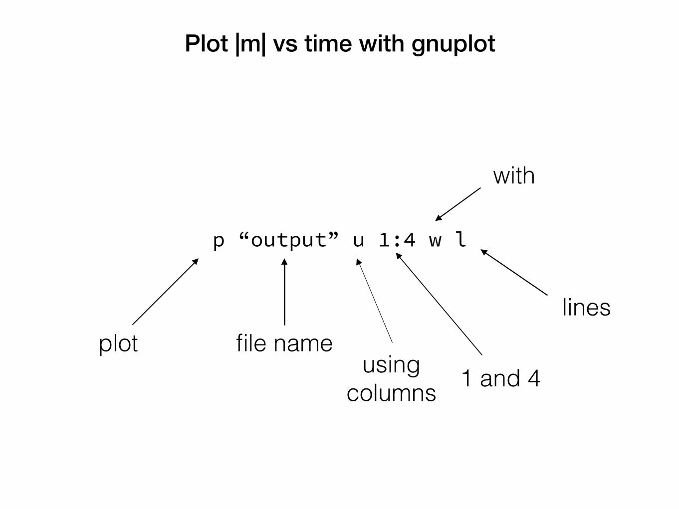
Plot |m| vs time with gnuplot

p “output” u 1:4 w l

plot file nameusing

columns 1 and 4

with

lines

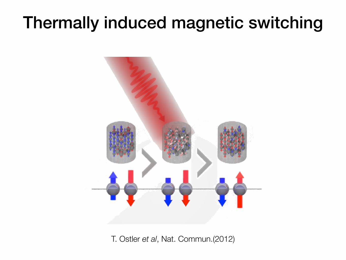
Thermally induced magnetic switching

T. Ostler et al, Nat. Commun.(2012)

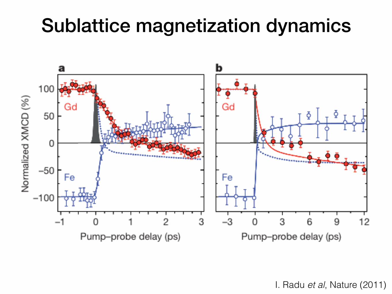
Sublattice magnetization dynamics

I. Radu et al, Nature (2011)

GdFe ferrimagnet

Gd Fe

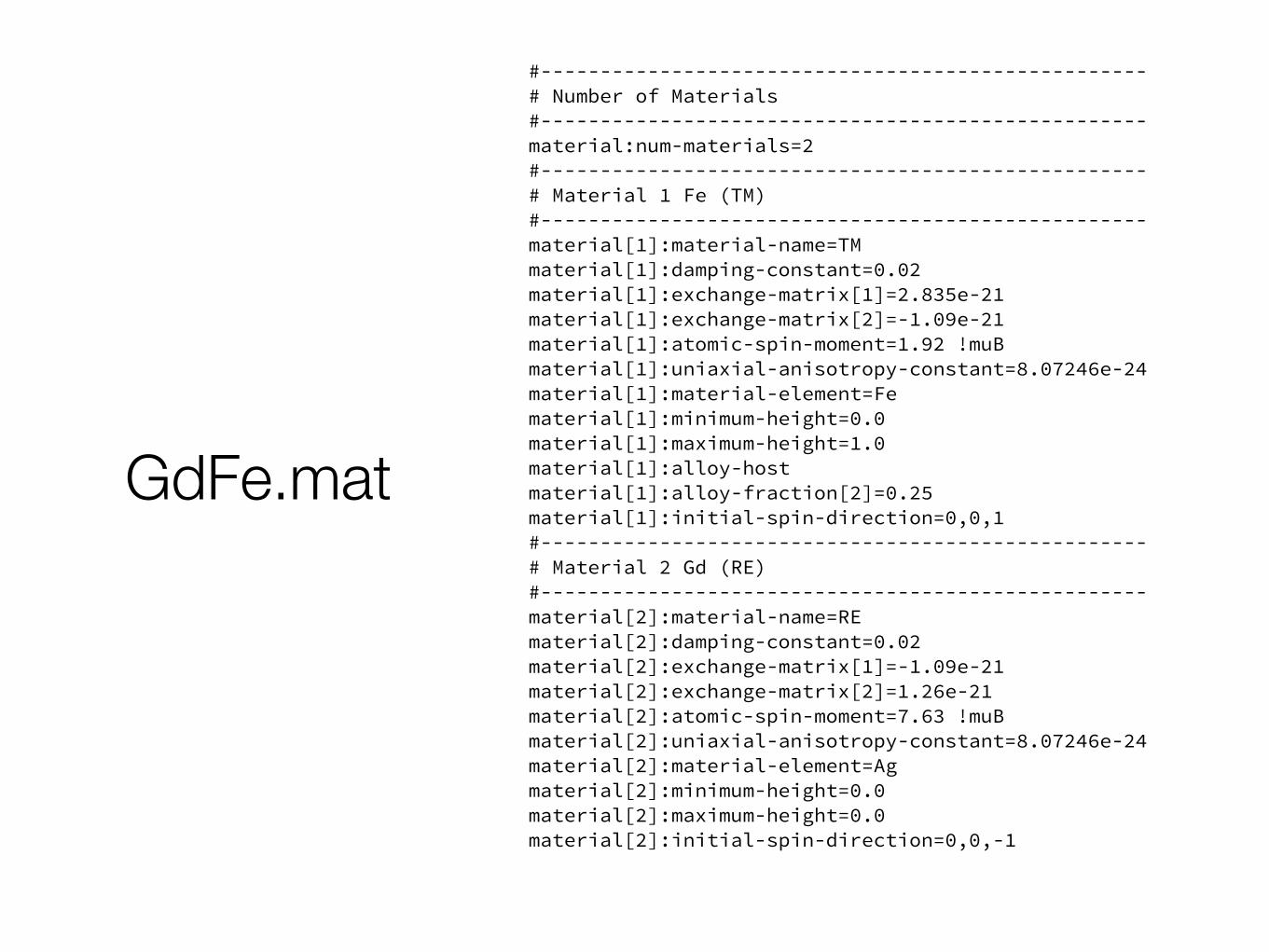
GdFe.mat

#--------------------------------------------------- # Number of Materials #--------------------------------------------------- material:num-materials=2 #--------------------------------------------------- # Material 1 Fe (TM) #--------------------------------------------------- material[1]:material-name=TM material[1]:damping-constant=0.02 material[1]:exchange-matrix[1]=2.835e-21 material[1]:exchange-matrix[2]=-1.09e-21 material[1]:atomic-spin-moment=1.92 !muB material[1]:uniaxial-anisotropy-constant=8.07246e-24 material[1]:material-element=Fe material[1]:minimum-height=0.0 material[1]:maximum-height=1.0 material[1]:alloy-host material[1]:alloy-fraction[2]=0.25 material[1]:initial-spin-direction=0,0,1 #--------------------------------------------------- # Material 2 Gd (RE) #--------------------------------------------------- material[2]:material-name=RE material[2]:damping-constant=0.02 material[2]:exchange-matrix[1]=-1.09e-21 material[2]:exchange-matrix[2]=1.26e-21 material[2]:atomic-spin-moment=7.63 !muB material[2]:uniaxial-anisotropy-constant=8.07246e-24 material[2]:material-element=Ag material[2]:minimum-height=0.0 material[2]:maximum-height=0.0 material[2]:initial-spin-direction=0,0,-1

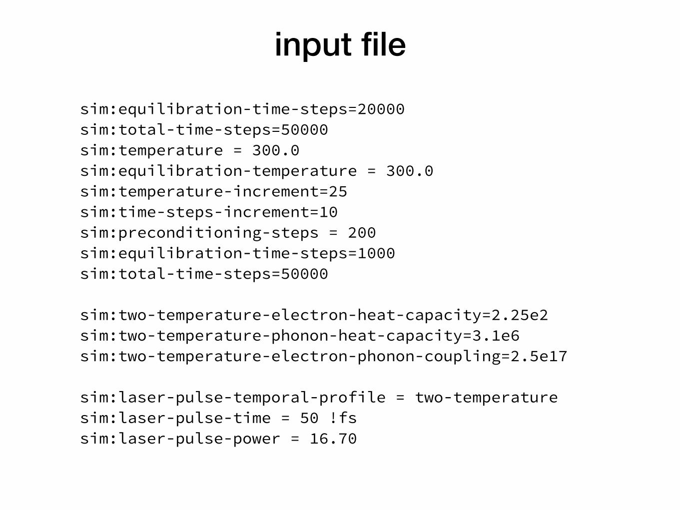
input filesim:equilibration-time-steps=20000 sim:total-time-steps=50000 sim:temperature = 300.0 sim:equilibration-temperature = 300.0 sim:temperature-increment=25 sim:time-steps-increment=10 sim:preconditioning-steps = 200 sim:equilibration-time-steps=1000 sim:total-time-steps=50000

sim:two-temperature-electron-heat-capacity=2.25e2 sim:two-temperature-phonon-heat-capacity=3.1e6 sim:two-temperature-electron-phonon-coupling=2.5e17

sim:laser-pulse-temporal-profile = two-temperature sim:laser-pulse-time = 50 !fs sim:laser-pulse-power = 16.70

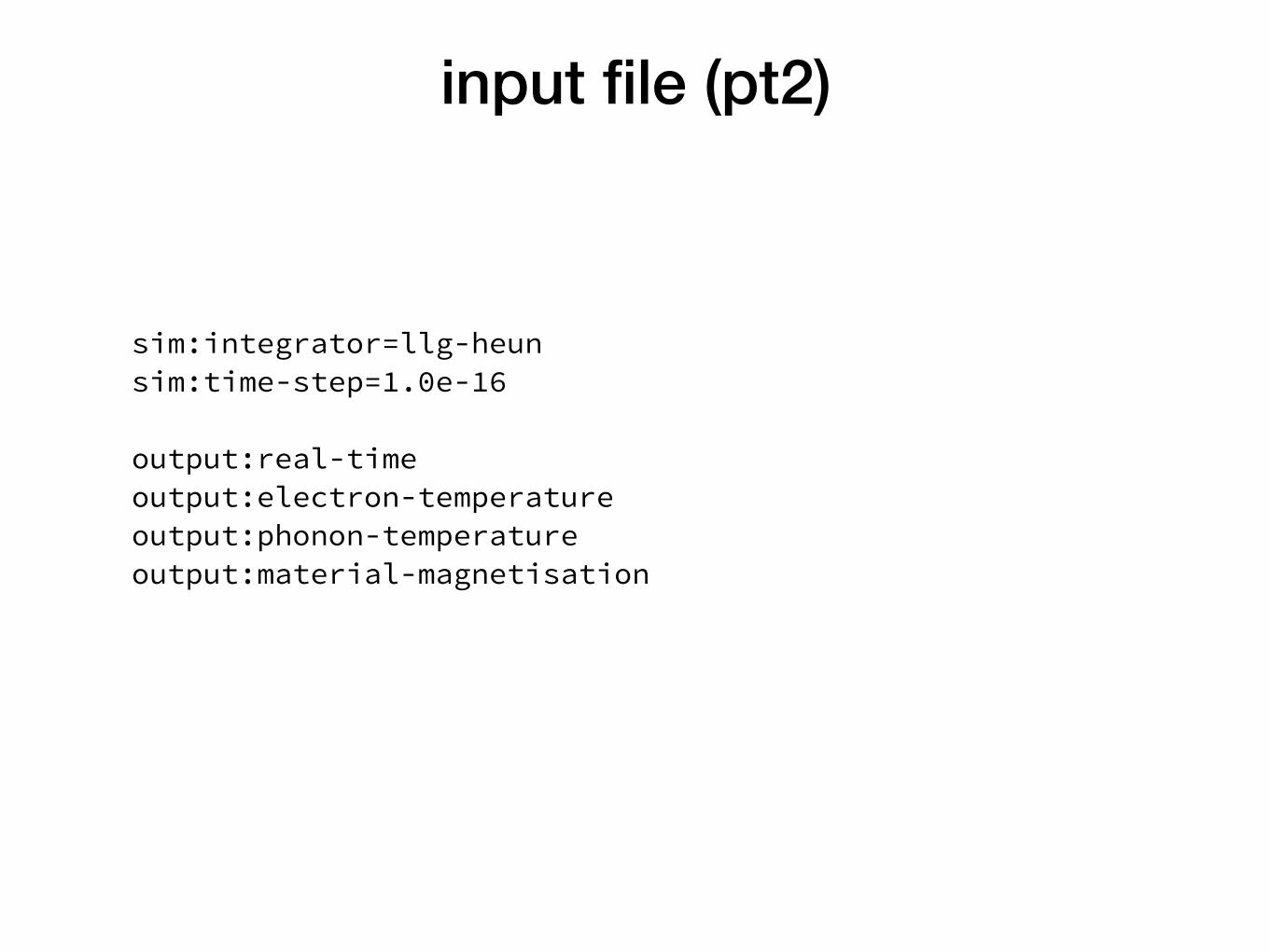
input file (pt2)

sim:integrator=llg-heun sim:time-step=1.0e-16

output:real-time output:electron-temperature output:phonon-temperature output:material-magnetisation

-0.8

-0.6

-0.4

-0.2

0.0

0.2

0.4

0.6

0.8

0 1 2 3 4 5

Norm

aliz

ed m

agnetiz

atio

n

Time (ps)

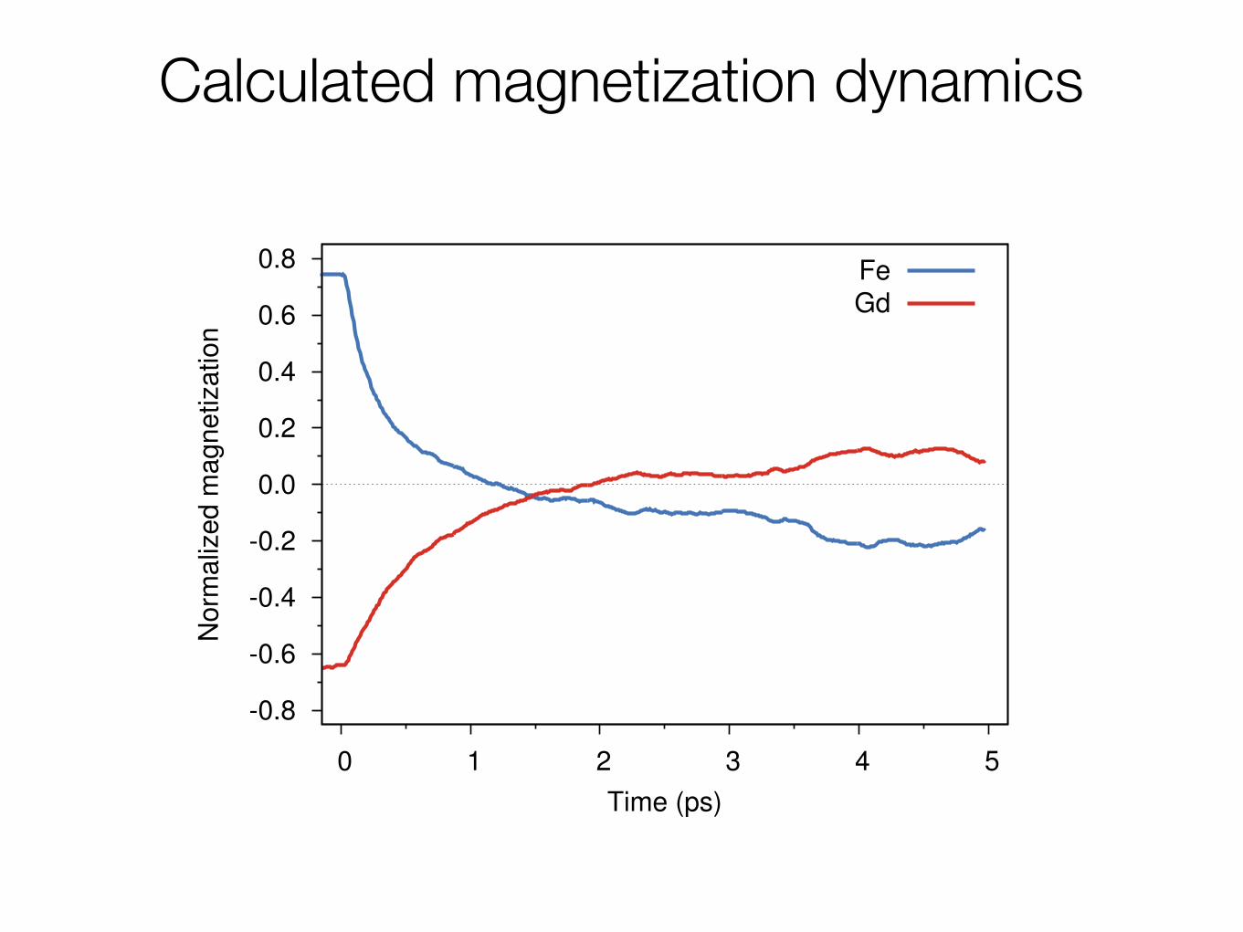
FeGd

Calculated magnetization dynamics

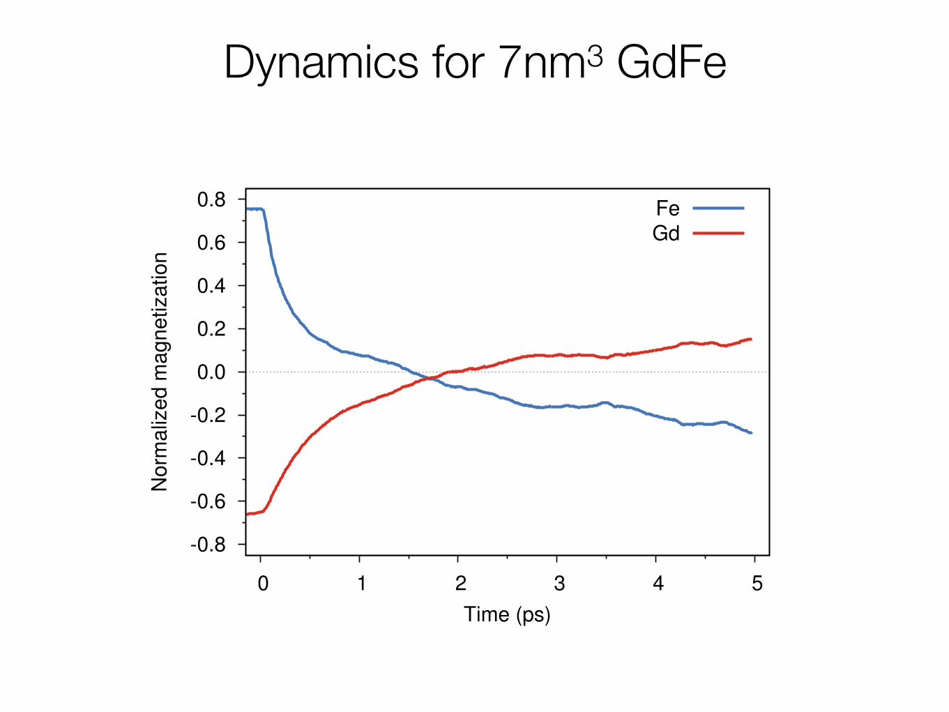
Dynamics for 7nm3 GdFe

-0.8

-0.6

-0.4

-0.2

0.0

0.2

0.4

0.6

0.8

0 1 2 3 4 5

Norm

aliz

ed m

agnetiz

atio

n

Time (ps)

FeGd

Summary

Simulated Curie temperature and demagnetization dynamics in Ni

Simulated TIMS in GdFe

Many different types of simulations possible (materials, alloys, multilayers…)

VAMP I RE

vampire.york.ac.uk