modeling thermal fire resistance

Build. Sci. Vol. 6, pp. 197-208. Pergamon Press 1971. Printed in Great Britain t(R6) [

Modeling Thermal Fire Resistance EDWARD M. KROKOSKY*

Computer-aided procedures have been developed to allow architects and engineers with no previous computer knowledge to prediet the theoretical fire ratings of different layers of fireproofing materials. The device which permits such a theoretical evaluation is a computer model known as FIRE (Fire Intensity-Resistance Evaluation). Using this procedure a engineer can choose up to three different layers of material to be evaluated under various fire intensities. The layers which can contain water or different transformation products can be considered to be in intimate contact or separated by an air gap. The various layers can be considered to be attached to a heat sink which represents the mass of various structural members of different sizes.

A direetory offifty materials is available for evaluation under.fire exposures of different intensities and durations. Correlations are now being carried out with existing fire tests to insure the best f i t for the different temperature- dependent material parameters that are required.

NOMENCLATURE

k., thermal conductivity for material m

q heat flux T temperature A x-sectional area p= density for material m c., specific heat for material m :t diffusivity 0 l,,,m thermal conductivity at point

iin material m 02,i,., specific heat density term at

point i in material m Ax= incremental spacing in

material m CBlt time dependent hot surface

boundary condition NI cold surface thermal co-

efficient--non-dimensional NF hot surface thermal coeffi-

cient-non-dimensional 02,N0,m specific heat density term for

the no-gap condition for material m

NG,. no-gap interface heat transfer coefficient for material m

h time interval step h, surface heat transfer coeffi-

cient t, M M time

* Associate Professor of Civil Engineering, Carnegie- Mellon University, Pittsburgh, Pennsylvania.

197

TTL INF

INI

TEMP[m, M M - 1, i]

CBF CB2 TTC GI[i]

M M - 1 N U MA T MAT1 MATHIC2

PERCENT3

PRINOPT CRITFT HSOPT HSNUM

HSTH NGAP

HH(1)

CBF(I)

MTT(LOOP)

thermal lag coefficient internal high temperature surface heat transfer coefficient internal low temperature surface coefficient temperature in material m, at time t - h at point i surface fire temperature ambient outside coefficient critical time constant slope calculation from R. K. Coefficient 1 at point i t - h number of material layers number of material 1 material thickness of material layer 2 percent of phase transformation material in layer 3 printout temperature option critical fire temperature heat sink option number of the heat sink material heat sink thickness gap between material layers option total time elapsed since the start of exposure fire exposure curve as a function of time material transformation temperature

198 Edward M. Krokosk v

THECOTRANS (LOOP)

THECOTEM (LOOP)

HAS

LOOP, M

thermal conductivity after transformation

thermal conductivity temperature factor heat-sink-surface heat transfer coefficient into the sink material layer

INTRODUCTION

Program aims

THE DEVELOPMENT of analytical techniques for predicting the fire resistance of different types of materials has not progressed rapidly. This is due to a lack of easily adaptable mathematical procedures for predicting the fire resistance of different material layers and a lack of thermal data on the large number of fireproofing materials currently in use. For the most part practicing structural and architectural engineers do not have the computer knowledge nor the time to carry out tedious numerical calculations to make such predictions.

In addition the increased development of new materials and construction techniques make it imperative that improved fireproofing evaluation techniques be developed. The increasing backlog of costly fire tests necessitates the development of analytical fireproofing techniques.

FIRE (Fire Intensity-Resistance Evaluation) was developed to meet these two basic requirements. It is a user-oriented procedure which simulates numerically the resistance of different fireproofing materials put together into arbitrary layers. The procedure as such is user-oriented in that it can be implementeedby apracticing engineer or architect with no previous computer knowledge. In addition the procedure could also be used as a research tool for predicting fire ratings of new constructions. The program makes use of temperature- dependent thermal parameters which may or may not correspond to the standard thermal parameters which are determined at thermal equilibrium.

Previous and future work in the field

Over the past few years very little analytical work has been done in the fireproofing field[I-3]. Several analog and numerical models have been tested, but poor accuracy, excessive time requirements, relative inflexibility, and a lack of thermal property data, have limited the usefulness of most of these models[4]. Furthermore, there has been a certain reluctance to use computational procedures for predicting the rates of heat and mass transfer.

This has resulted in an inordinate burden on testing, with the result that large numbers of costly fire tests have to be run. It is hoped that the development of models will reduce a large number of repetitive tests.

With this model it is envisioned that many potential materials and countless material combina- tions could effectively be tested without the expense of undertaking actual fire tests. New materials could also be screened initially in this model and proposed fireproofing materials could be tested even before they are manufactured so that their fireproofing potential could be evaluated before costly production starts.

Fireproofing

Effectiveness of fireproofing materials. The main practical criterion for judging of the effectiveness of fireproofing materials is the fire endurance test, where the specimen with its applied load, if any, is tested until failure occurs or until the specimen has withstood the test conditions for the allowed period of time (ASTM designation: E 119-67)[5]. Some- times other aspects also have to be weighed in fireproofing evaluations. One test on walls is the hose-stream test where a specimen is subjected to a fire exposure test for one hour, then immediately subjected to the impact, erosive and cooling effects of a specific stream of water.

Fireproofing around structural members can be tested either with a superimposed load on the member which approximates as nearly as possible the working stress in each member, or the specimen can be tested without load. Temperatures of the structural elements must not exceed 1200°F at any one of their surface points.

When combustible materials are in contact with the structural or fire-proofing materials, the temperature increase at the points of contact cannot exceed 250°F[5]. The fireproofing material should withstand the fire endurance test without ignition of the protecting material for at least the length of time for which the classification is desired. In masonry, concrete and other incombustible materials the maximum permissible temperature on the nonfire face is 325°F. This temperature and other temperatures cited in this section are defined as the critical fire temperatures.

The material should be representative of the quality of construction and workmanship that wilt be found on the actual job site.

Fire Curve Selection and Fire Loads. Since 1918 the standard "fire curve" (i.e., the assumed temperature-time exposure for t h e building element) has been the ASTM E 119-67 curve[5]. This curve assumed a long fire duration with steadily increas-

Modeling Thermal Fire Resistance 199

ing temperatures for at least 8 h. The ASTM curve represents the fire severity likely to occur in the complete burnout of the contents and the structure of a typical brick, wood-joisted building. But today, many potentially dangerous fires occur in an environment totally different from the one for which the fire curve was developed.

Several European experimenters have investi- gated fires which followed the ASTM curve rather closely initially, but failed to maintain a high intensity for a long period of time[6].

Other studies comparing the observed fire curves and the standard ASTM curve show that contrary to the ASTM standard, the fire often reaches a peak early in its history, then fails gradually to a fairly constant value. This high temperature and the time it takes to achieve it depend a great deal on the amount of air available for combustion through window openings (ventilation). One of the most obvious factors affecting fire severity is the amount of fuel supplied to it by the combustible products such as decorations, furniture, furnishings, and various combustible materials. The amount, nature and distribution of these combustible products can be measured for a given type of building or apartment. The total caloric value of this fuel is called the "fire load" of the building. When the fire load is divided by the floor area, it is called the "fire load density", which is usually converted into an equivalent weight of wood. The units for this are so many pounds of wood per square foot. For the average domestic building (hotel, office, etc.) the fire density should not exceed 12 lb/ft 2. The average fire load density obtained for apartments and residences is in the 8.8 lb/ft 2 range, while the range for offices is 3.8 to 16-7 lb/ft2[7].

Considering these uncertainties, two different fire curves along with the standard ASTM curve were elected as the temperature inputs. (See figure 1.) It can be seen that the higher the fire load density, the higher the temperature reached by the fire.

Model capabilities

Using the standard ASTM fire curve or any desired fire intensity input, the numerical model will predict the temperature as a function of time for various positions in up to three layers of protective material attached to a structural member with various interface conditions. The procedure pre- cludes the occurrence of decomposition or combustion of the insulating material.

The insulation material in question can have the following variable properties:

1. surface conductance 2. diffusivity 3. thickness 4. thermal conductivity 5. specific heat 6. surface heat transfer coefficient 7. density 8. moisture content 9. material transformation potential

Various insulation layers may be considered to be affixed to a high thermal conductivity mass which will absorb heat but will support no temperature gradient.

The program structure can be divided into three main parts:

1. primary setup and implementation 2. computational procedures and evaluation 3. solution printout procedures

In the primary setup and implementation segment, the necessary properties are defined and the material properties, curve coefficients and material dimensions are entered. From this data, the density, thermal conductivity, specific heat, thermal diffusivity and critical time steps are computed and put into a form compatible with the program requirements. These values are subsequently printed out in the first part of the program.

The computational procedures are cycled a prescribed number of times depending on the number of fireproofing material layers present.

22oo[ 12.4(1/4 ve.t,otion) e

's°°t °"°°r/J \

.............. .X "ooi "'o"oo' 2ooF! -- __ es" .

o 1400

60~

0 10 20 30 40 50 60 70 80 90 t00 tt0 T i m e - ra in .

Fig. 1. Different fire curves intensity inputs.

480

200 Edward M. Krokosky

The basic computation element employs a Runge- Kutta Gill procedure which is used to numerically integrate the heat transfer equation after it has been set in the finite difference form. The smallest critical time step size is automatically determined in the case where several different materials are used. The Gill error control system operates in this phase of the program and checks the Runge-Kut ta method for accuracy. I f the values are acceptable, they are stored in a multi-dimensional matrix for a later printout. The procedures are then repeated for the desired time duration.

Solution printout procedures involve various listing and graphing techniques for presenting the prescribed data. Various options can be employed to control the time interval for which the data will be printed or punched out.

The present program is written in ALGOL and is presently available on a UNIVAC 1108 computer at Carnegie-Mellon University.

MATHEMATICAL ASPECTS

General mathematical considerations

Basic heat transfer equations. The simplest possible heat diffusion consideration is one in which the heat is transferred from a region of higher temperature T , to a region of lower temperature T L over a distance dx under steady state conditions. In this case, since T n and TL are constant, the gradient dT/dx is constant. Solutions of problems of this type are based upon the empirical expression[8]

q dT - k - - ( 1 )

A dx

where q/A is the heat flux. More commonly, the situation arises where the

temperature gradient is a function of time. Under these unsteady-state conditions, both the gradient dT/dx and the heat flux change with time. This behavior can be represented mathematically by the expression[8]:

sT I = a ( 2 ) ~t / c?'c2

where ~, the thermal diffusivity, is given by

k :e = - - (3)

pc

The temperature gradient through the fireproofing material is initially non-linear and will gradually become linear and constant if the boundary conditions do not change and if, for example, thermal conductivity and other thermal

properties are not a function of temperature or time. If these conditions exist then the temperature will eventually not vary with time at fixed points within the body. This condition is called "+steady- state conduction" and under these conditions ~T/~t = 0.

Several methods exist tbr solving the parabolic heat transfer equation. The method employed here involves reducing equation 2 to an ordinary differential equation by using a finite difference approximation for the second order term[9].

Figure 2 shows the resulting finite difference grid for computing the temperature at discrete points within the fireproofing material.

,~Ax ~ax~

Fi~,. 2. Typk'al finite difference grid fi," one material &yer.

Boundary conditions. The rate of heat influx through the various boundaries is handled by means of surface heat transfer coefficient, hr. The surface heat transfer coefficient is independent of the thickness of the various boundary films that surround any solid surface and can be thought to be made up of both convective and radiative components. Since the rate of heat transfer on the fire surface is thought to be primarily radiative an appropriately high radiative heat transfer coefficient is chosen. Previously conducted simulation work indicated that a constant time and temperature independent coefficient would not introduce too great an error[4]. This is not to imply that a time-temperature dependent heat transfer coefficient cannot be implemented if it is deemed necessary.

Material phase transJbrmations. Not all the heat that an object receives causes a rise in its temperature. Large amounts of energy are needed to do the work of separating the molecules when solids change to liquids and liquids change to vapors. To raise the temperature of one pound of water from 63°F to 64°F requires one British Thermal Unit (B.t.u.). The amount of heat per unit mass necessary to change a liquid from the liquid to the vapor phase without a change in temperature is called the heat of vaporization. The heat of vaporization is usually measured at the normal boiling point of the liquid. For water, the heat of vaporization is approximately 970 B.t.u./lb. This is over five times as much energy as is needed to heat water from the melting to the boiling point.

Thus it can be seen that a definite temperature lag can occur when a fireproofing material containing


water is subjected to an increasing temperature. This transformation temperature lag (latent heat of transformation) is expressed mathematically by:

TTL = (latent heat) (~o moisture)/(specific heat * 100) where specific heat is for fireproofing material in which the water exists or transformation product exists. The units for TTL is in degrees of temperature.

In the case of water, this lag manifests itself when the temperature at a specific point in the material rises to 212°F. When this happens, a "temperature plateau" is reached where the temperature levels off as the moisture is changed into vapor. The temperature will remain stationary until all the moisture in that particular segment is changed into the vapor state; then the temperature at that point will again start to rise.

Phase changes, because of the large quantities of heat involved, can be extremely effective in con- trolling the heat rise in the fire-proofing material[10].

Property changes with temperature. It is well- known that the thermal material properties like thermal conductivity and specific heat change as a function of temperature. These changes may be more pronounced after a transformation has taken place, e.g., in the case of concrete when water transforms at 212°F there is a pronounced change in the thermal properties after transformation. Not only is there a pronounced change after a transformation, but in addition there may be a change in the thermal parameters with temperature. Limited experience has indicated that the thermal conductivity is the most temperature sensitive parameter with specific heat and density following in that order.

In the finite difference model one set of thermal parameters has been used to describe the behavior each material layer. Computationally it would have been possible to have a different set of thermal parameters for each segment of the finite difference model. However, at this state of the model development it was not felt that this additional computational complexity is justified. Since it is easier to monitor the temperature data at one point in a

material, changes in the thermal properties as a function of temperature are governed by changes at this point for the whole material layer. This essentially means that the thermal temperature factors are based on one given temperature in the layer. However, one layer may be broken up into sublayers as in the example given,if the temperatures are measured at intermediate points throughout the thickness. How realistic these thermal parameters are when compared to equilibrium thermal parameters is not known at this time. Because of the transient nature of the temperature exposure the use of these thermal model values is not any more questionable at this stage than the use of often non- existent thermal parameters which are determined by experiments carried out at equilibrium.

Thermal parameters considered. Seven thermal parameters are considered depending on whether a material transformation is present or not. If no material transformation is actually present a pseudo-transformation is considered to bring temperature-dependent parameters into the computation process. The seven parameters that are considered are:

(1) density (2) thermal conductivity before transformation (3) specific heat before transformation (4) thermal conductivity after transformation (5) thermal conductivity temperature factor (6) specific heat after transformation (7) transformation product

Table 1 indicates the computer notation equiv- alents for the parameters and their respective units. It should be noted that there is no temperature- dependent factor for the specific heat. A factor could have been introduced but since the thermal conductivity is generally more sensitive to temperature than the specific heat and since from a computational standpoint the temperature-dependence of the specific heat is divided by the temperature-dependence of the thermal conductivity the introduction of an additional factor is not justified. Furthermore it emphasizes that the

Table I. Thermal parameters

Thermal Parameter

of the simulation model

Computer Notation Equivalent Units

Density Thermal conductivity before transformation Specific heat before transformation Thermal conductivity after transformation Specific heat after transformation Thermal conductivity temperature factor Transformation product

DENF lb/in, a THERMCOND B.t.u.-in./ft2-hr-°F SPECHEAT B.t.u./lb-°F THECOTRANS B.t.u.-in./ft2-hr-°F SPECTRANS B.t.u./lb-°F THECOTEM B.t.u.-in./ft2-hr-°F 2 PERCT Ib/lb-100

202 EdwardM. Krokoskv

parameters introduced here are model parameters and that these values may or may not coincide with the thermal equilibrium temperature-dependent values of thermal conductivity, specific heat and density.

The various thermal parameters are stored in a materials directory of fireproofing materials. This directory contains the best known thermal properties for the materials in question. The thermal parameters that are stored in FIRE are determined by a special computer program[11] which analyzes the data from some carefully regulated experiments. This program determines the appropriate thermal parameters by an optimization search routine.

The thermal conductivity that is used in the computational procedures after transformation is arrived at by:

THECOTRANS (LOOP) ~ THECOTRANS (LOOP) + [TEMP (LOOP, MM-1, 9 ) -

MTT (LOOP)] * THECOTEM (LOOP) (4)

Finite differences

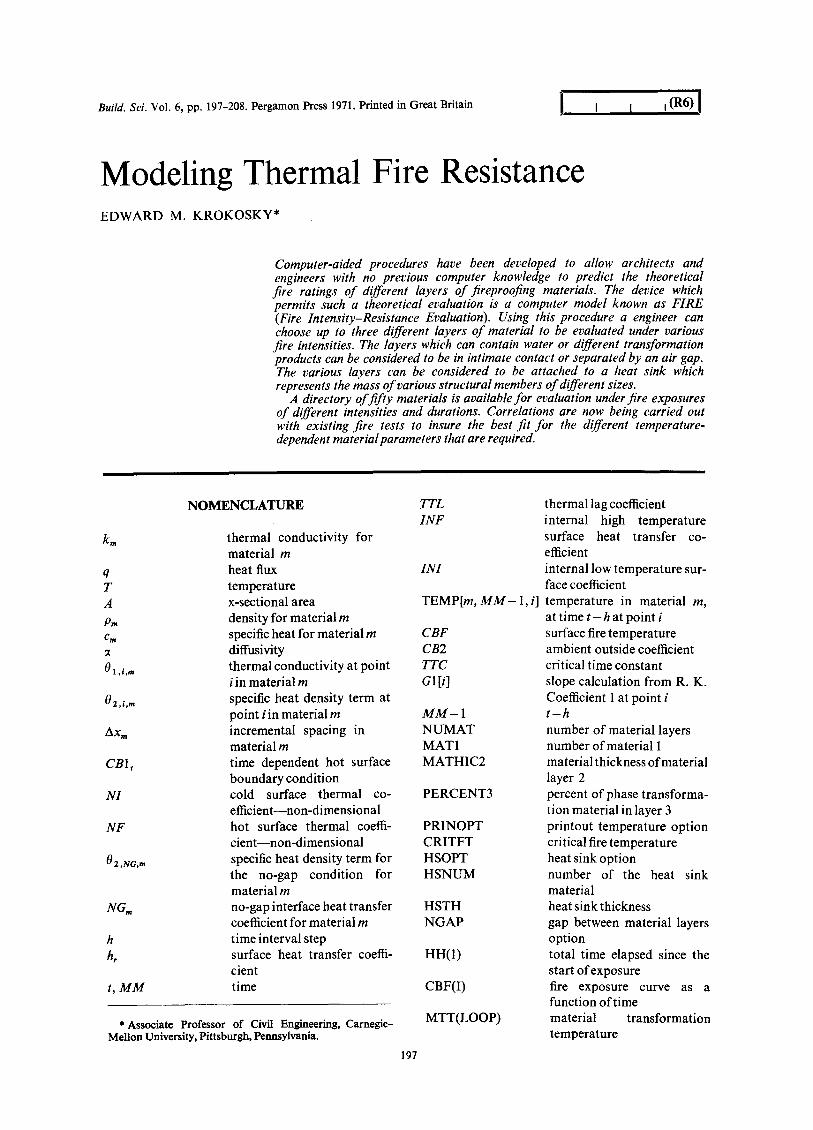
Normal interfaces. In order to accomplish the numerical solution of the partial differential equation, governing heat transfer, it must first be rewritten in the finite difference form. By dis- cretizing the spatial derivatives, the partial differential equations become a system of simultaneous ordinary differential equations which are amenable to solution by numerical integration techniques[12]. The discrete spatial segments of the various fire- protective layers insulation can be seen in figure 2. Using the second order central difference approximation the heat transfer equation becomes:

0201'~'m[ Ti- l'm-2Ti'"+ T'+ l'" .... ~ _ dT~,,,at (5)

for interior poinls, where the i subscript refers to position and the m subscript to the material layer.

The finite difference equations take on a different form at points adjacent to the boundary. At point 1 the term T;_ J,m refers to the boundary conditions at the fire surface, while at point 9 the term Ti+ 1,,, refers to the interior boundary conditions. Thus the finite difference equatioqs become:

At point 1 or the high temperature boundary

02.0"I"ICBI'-TI'm(l+NF)+T2"],.m AxZ~ - dTl"mat (6)

where CB1, = NF. CBF(t); At point 9 or the low temperature boundary

O,,9.,,[T8.m-Tg,m(I+NI)+CB2t'] dT9 ,m

02,o, m] Ax~ ] = dt (7)

where CB2t = NI. CB2.

The choice of nine points in the insulation was not arbitrary but was governed by the relative material constants of fireproofing materials and the approximate thicknesses encountered in insulation materials. The choice of nine points governs the value of Ax which, when used in conjunction with the material properties, effects the characteristic time constant for the problem. This time constant controls the accuracy and stability of the numerical integration. In addition, there must be enough finite difference stations to give a clear picture of what is happening throughout the fireproofing insulation. The choice of nine integration points fulfilled both these conditions.

No-gap interface. In order to simulate the condition of perfect contact of material elements certain changes were made in the previously described material constants used in the pro- grammed equations. To maintain the symmetry of program and to reduce the extent of programming repetition the temperatures on both faces of the material elements were computed. The equations were modified in such a way that temperatures computed on both surfaces of an infinitely small gap were identical, i.e,, perfect contact was assumed. Equations 8 and 9 show some typical modifications to the existing gap equations. Figure 3 shows the model used for calculations.

\ l l l I l ° l ° . . . . / (~ (~ t,Z t,3 4,4

T, , ! : Tt, 2

Fig. 3. Typical finite element grid for material layer one and two assuming perfect material contact (no gap).

On either side of the existing gap between materials one and two the basic equations are now

01,9,1 [Ts , , - To,I(I + N____G,)+ Tz,2NG,] = dT9,1 02.u~.1 Ax~ dt

(8)

where NG~ = k2/k~ and T9,~ is the interface temperature. For the other surface

02.s~,202'2"2 LIT1"2NGz- T1'2(I~ + NG2)+ T2 ,j21 = dTl,2dt

(9)

where N G 2 = kl/kz and T1, z is the identical surface temperature. 01,9,m and 02,1,,, are identical to other terms defined in equation 5 while 02,i,,, terms have to be modified to account for an average heat capacity of the center section. The actual temperature at the interface is the average of the T9,1 and TI, 2. Numerical computer checks indicate


that with an order of magnitude difference in the thermal diffusivity and a factor of two difference in the thickness the temperatures differ by a 0"5°F for a temperature change of 150°F per hour. For temperature changes of 10°F per hour and an order of magnitude difference in the diffusivity and a factor of two difference in the thickness the temperatures are identical.

Heat sink option

When using materials of high thermal conductivity, the critical time step becomes quite small. It is necessary to avoid extremely small time steps because of the excessive computer time requirements. In some fire exposures in which structural elements are being protected the large structural elements have high thermal conductivities relative to the protective fireproofing material. However, the mass of these elements is critical in the final fireproofing evaluation. In order to save computer time in exchange for accuracy the Heat Sink Option is available. This option assumes that all the heat from the back surface of the insulation is stored in a heat sink which loses no heat. It is also assumed that the back surface of the insulation sees a constant temperature.

The surface rate of the heat transfer into the mass can be controlled by a surface resistance, HAS. If none of these assumptions is acceptable and the user desires more accuracy, then the No-Gap Option with the metallic material as one layer should be used in lieu of the Heat Sink Option.

Gill error control. The Gill Error Control[13] is executed between various time steps. It is respon- sible for insuring that the numerical integration is compatible within certain acceptable error limits, from station to station and from one time step to another.

The initial values assigned as data to the system constitute the initial gradient in the fireproofing material. For a given time step four sets of gradients are calculated from the finite difference equation. Each of three of the four calculated gradients depends on a previous gradient. These four gradients have to meet a certain error control criterion.

ERR(i) = ABS I G3(i ) - G2(i)/G2(i)- GI(i) ] (11)

In this program, ERMIN = 0.00001 and ERMAX = 0.4. If ERMAX comes out to be larger than the allowed value, then the time step of the program is immediately halved. The system is then initialized and the calculations are resumed with half the original time step.

COMPUTER ASPECTS

Overview of the computer segments

Figure 4 gives an overview of the various basic computational elements that presently exist in the program as of April 1970. Additional refinements of the program are continually being made in order to accommodate the requirements and desires of the various users.

Numerical solution of first-order differential equations

Numerical integration. The Runge-Kutta[12] numerical integration procedure was chosen for the solution of the system of simultaneous ordinary differential equations. The nine points chosen as integration stations are shown in figure 2. The integration routine uses Kutta's fourth-order processes in which the error in each step is of the order of At 5 where At is the length of the time interval. It has the desirable feature that no values are necessary beyond one time increment in the past.

The choice of an appropriate time step for integration is a critical factor. A poor choice may result in an unstable integration sequence with no assurance of convergence. Normally a good value for the time step for this type of parabolic equation is 10-15 per cent of the smallest time constant of the problem.

The time constant for the temperature equation is

TTC(m) = 02,~,m (Ax 2) (10) 01,i,ra

Repetitive programming elements

In order to reduce the size of the computer program a certain basic computational segment was used for each fireproofing material layer. This basic segment involved the calculations required for computing the heat transfer through one material layer. Heat transfer through successive fireproofing material layers used the same program element with varying boundary conditions. Table 2 gives the varying boundary conditions as the number of material layers increases.

Fire curve generation

In the procedure call as it now stands there exists the option of using the so-called standard ASTM Fire Curve E 119-67 or two other fire curves. Fire curve one (1) is a high temperature short duration fire curve, while fire curve three (3) is a low temperature long duration exposure.

The standard fire curve is generated by a ninth- order polynomial in the region of extreme curva- ture. The standard fire curve has been segmented four times for maximum accuracy. Figure 5 shows

PROCEDURE DEFINITION FIRE ( ) $ PROCEDURAL VARIABLES

I STORE FIRE CURVE

COEFFICIENTS

I STORE FIRE MATERIAL

PROPERTIES

I ASSIGN FIRE COEFFICIENTS

I ASSIGN SURFACE

COEFFICIENTS

I TAKE PROPERTIES

FROM MATERIAL DIRECTORY

I COMPUTE CRITICAL

TIME STEP

I BASIC REPEAT FOR TIME INCREMENT

I COMPUTE

FIRE CURVE

I COMPUTE SURFACE

COEFFICIENTS

I COMPUTE THERMAL TRANSFORMATION

TEMPERATURE

I START LOOK FOR

NUMBER OF MATERIALS

I REASSIGN COEFFICIENT FOR EACH MATERIAL

SEE TABLE

I START NUMERICAL

INTEGRATION FINITE DIFF. PROCEDURES

I FINITE DIFF.

PROCEDURES

I PICK CRITICAL TIME

STEP

I INITIATE TEMPERATURE

VALUES FOR EACH TIME INCREMENT

I CALCULATE FIRST

RUNGE-KUTTA STEP USING PROCEDURE CALCULATION

CALCULATE SECOND RUNGE-KUTTA STEP USING PROCEDURE CALCULATION

I CALCULATE THIRD


I I

j I CALCULATE FOURTH


I _ CHECK GILL ERROR

CONTROL

I CALCULATE NEW

TEMPERATURES AT EACH POINT IN ONE MATERIAL

I CHECK TRANSFORMATION

TEMPERATURE LEVEL

I DELAY FOR HEATS

OF TRANSFORMATION IF NECESSARY

I t ~ RETURN FOR NEXT

MATERIAL LAYER

I CALCULATE HEAT . . . . . .

TEMPERATURE IF APPROPRIATE

I CHECK CRITICAL

FIRE TEMPERATURE TERMINATE PROGRAM

IF NECESSARY

I

t~ RETURN FOR THE NEXT IME INCREMENT IF TOTAL

EXPOSURE TIME HAS NOT BEEN EXCEEDED

I VARIOUS PRINTOUT

OPTIONS

Fig. 4. Ocerriew o[ computer program fire.

Table 2. Boundary parameter changes as a function o f material layer,~

C B F i . . . . . . . . . . . . . . . . . - - i - * N l

• CB2 "NFI H A l H A 2

- - - C B 2 . . . . C B 2 . . . . CB2

I i " 2 ° 3 ° -I . . . . . . . . I -~

INI[2] INF[2] INI[3] INF[3]

N u m b e r

o f

Material layers

CBF N F CB2 NI

CBF N F CB2 NI CBF N F TEMP[2, INI[2]

M M - 1 , 1] CBF N F TEMP[2, INI[2]

M M - I , 1]

Material Layer*

2 i 3

C B F N F CB2 ! NI CBF N F CB2

x x x x x TEMP[1, INF[2] CB2 i NI x

MM,9] T E M P [ I , INF[2] TEMP[3, INI[3] TEMP[2,

MM,9] M M - 1, I ] MM,9]

X X

X X

INF[3] CB2

* Term x indicates not required.

N I

X x

N i


2~'00

1800

U. o

® 1 4 0 0

o

1 ooo E

60(3

200

0

• , polynomiOt ~, L . i n e a r ~ pol~nomlC,~ , To D ~ To De r e e ~ , ~ ~

1 I i

,~Linear Approximation

I I I L 0.5 t .0 1.5 2.0

Time-hours

Fig. 5. Breakdown of various Regions of the fire curve for Polynomial approximation (see appendix 2).

the breakdown for the standard curve as generated by the computer.

Fire curves (1) and (3) have been segmented three times. The intermediate region is approximated by a ninth-order polynomial while the initial and terminal portion are approximated by linear segments. Fire curve (1) corresponds to a fire load of 1.55 lb/ft 2, one-half of the area open for ventilation, while fire curve (3) corresponds to a fire load of 12"41b/ft 2, one-quarter of the area open for ventilation.

The polynomial coefficients for the standard fire curve ASTM E 119-67 are given in Appendix II.

Printout options

Various printout options exist. If it is only necessary to tell if the fireproof construction temperature has exceeded the critical fire temperature, then an option can be exercised and no temperature profiles are printed out. The only information printed is whether or not the critical fire temperature has been exceeded in the unexposed surface of the last material element. Certain options also exist for the computer graphing of the various temperature profiles.

P R O G R A M I M P L E M E N T A T I O N

The computer program consists of many distinct elements each designed to implement the evaluation of the fireproofing effectiveness of various material elements.

Procedure call

The program as it has presently been written requires no previous knowledge on the part of the user of any computer language. In its present state it consists of a procedural call in which the user simply has to put certain arguments into a call named FIRE. A typical call would be

FIRE (3, 8, 39, 11, 13-5, 38.5, 120.0, 0.0, 0.0, 0.0, 2, 1,800.0, O, O, 0-0, 1)$

where the procedural definitions are given below as follows:

FIRE (NUMAT, MAT1, MAT2, MAT3, MATHIC1, MATHIC2, MATHIC3, PERCENT1, PERCENT2, PERCENT3, FIRECURVE, PRINOPT, CRITFT, HSOPT, HSNUM, HSTH, NGAP)$ REAL MATHIC1, MATHIC2, MATHIC3, PERCENT1, PERCENT2 PERCENT3, CRITFT, HSTH $ INTEGER NUMAT, MAT1, MAT2, MAT3, FIRECURVE, PRINOPT, HOSPT, HSNUM, POPUT $

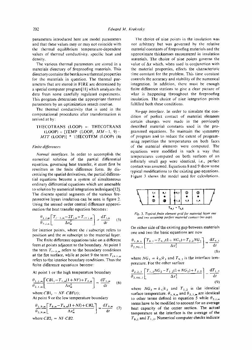
Table 3 gives information about each argument. Appendix III shows a typical computer program necessary for the complete call.

T Y P I C A L SIMULATION OUTPUT

Single layer systems

Figure 6 shows the simulation geometrics for the two cases studied. The results for a single layer of a siliceous aggregate concrete[14] ranging from 1-1/2 to 7 in. in thickness are shown in figure 1. The model contains provisions for changes in the thermal properties with temperature-dependency for this simulation. The thermal parameters used are given in Table 4.

Triple layered systems

Figure 6 shows the geometry of the simulation run for two layers of fireproofing material with no gap. This is in reality three layers because one layer was broken in two equivalent layers. The results for the Underwriter's Laboratory Test Material-B are shown in figure 8.

It should be noted that the simulation times are only for half an hour for case 2. This is because of a limitation on computer time which is imposed by the physical constants of the problem• The typical time step of 0.0001 hr has to be imposed for the case 2 problem consisting of three layers. This results

206 Edward M. Krokosky

Table 3. Various arguments for fire procedure

Argument

N U M A T M A T I } MAT2 MAT3 MATH1CI } M A T H I C 2 M A T H I C 3 PERCENT1 } P E R C E N T 2 P E R C E N T 3 F I R E C U R V E

P R I N O P T

C R I T F T

HSOPT

H S N U M HSTH

N G A P

Type of Variable

l* I I I R* R R R R R I

I

R

1

1 R

Funct ion

Number of mater ial layers

N u m b e r of the material chosen from the directory for layer number I to 3

Range

1 3 1-50 1-50 1-50

Thickness of each material layer f rom I to 3 0.25 -10

Per cent of phase t ransformat ion material in material layer 1 to 3 0-30%t-

Intensity of exposure I , 2, 3 I 1 -= Printout of temperature profile I or 0 I 0 = No pr intout of temperature profile

Critical fire temperature 1-2000 f 1 =- Heat sink present (must supply H S N U M , HSTH/ I or 0 I 0 -= No heat sink present

N u m b e r of heat sink material Thickness of heat sink

J 1 --= Perfect contact no gap 1 or 0 I 0 =- Gap between layers

* 1 = Integer R = Real.

t By weight.

80*F

t ...... @ / Material No, Concrete

l F i r e

I Case 1- Concrete Slob | ~ to 7 Inches Thick

Material No. (~ )4 .5 in . ® ~._~.,~j~n('~'~ J..Oin~__ Thin Steel Plate

Material

Material No. O t.O in. /

f Fire

• =Therrno Couple Location-Ref No. Case 2 - Underwrltere Material B - T h i c k n e s s Shown

Fig. 6. Various geometries employed in testing model.

Table 4. Thermal parameters used in model for cases 1 and 2

Material D E N F T H E R M C O N D

lbs/in. 3 B.t.u.-in./ft2-h-°F

Siliceous Aggregate Port land Cement

Concrete 0.0870 12.6 Underwri ter ' s

Labora tory Material B 0.0105 0.55

Thermal parameters

S P E C H E A T T H E R M O T R A N S S P E C T R A N S T H E C O T E M B.t.u.-in./

B.t.u./lb- F B.t.u.-in./ft2-h-°F B.t.u./lb-"F ft~-h:~F

PER CENT*

0.10 1.2 0.15 0.150 10%

0.200 0.55 0-200 0.006 0-01

* Trans fa rmat ion p roduc t - -970 B.t.u./lb-212°F.


E O Fire Simulator I-- - - Experiment

I I I 2 3 4

Time- Hours

Fig. 7. Simulation of heat transfer through siliceous aggregate concrete slabs of different thickness.

30

,,, 2 4

i ®

(~) Thermo Couple Locat ions

(See Fig. 7 ) I I I

0 200 400 600 800

Temperature -°F

Fig. 8. Results for case 2, Underwriter's Material-B.

in a computer run time on a UNIVAC 1108 of 540 sec for a 30-rain simulation. Any change of this time step towards a larger value results in loss of accuracy and instabilities. In the case 1 problem consisting of one layer of concrete for thickness in excess of 5 in. the critical time step was of the order of 0.001 hr. For this case 98 sec of computer time was required for a 130-min simulation. It is quite evident that critical time steps used in each program determine whether the model is a viable computer method for predicting fire resistance performance of layered materials.

C O N C L U S I O N S

It should be emphasized that the procedures set forth here are suitable only for preliminary estimates of the fireproofing efficiencies of layered materials. There is a definite indication that for some material systems a modification of thermal properties with increasing temperature will have to be made. This is especially true in material systems where a material transformation has taken place and the material properties are altered after the transformation.

The thermal parameters used are model parameters and should be construed as such. The fact that the same thermal parameters can be used for a range of concrete thicknesses, I-1/2 to 7 in., indicates their general utility. It has also been shown that the factors can be used to model intermediate data points in different layers of the same material. Whether this can be done for all materials

will depend to some degree on the sensitivity of the thermal material parameters to temperature and temperature gradients. The program however provides an excellent means to check how sensitive the thermal parameters are to temperature and thermal gradients.

The model as it now has been formulated provides an excellent means of estimating the potential and efficiency of layered material systems which are subjected to a variety of the fire exposures. This can now be easily done by the practicing engineer or architect with no previous knowledge of digital computers.

Acknowledgment--The author wishes to express his appreci- ation to J. R. Beyreis of the Underwriters' Laboratories, Incorporated of Northbrook, Illinois for his support and encouragement over the past year and for his aid in verifying the program by providing the output data from existing fire tests.

0 < HH[1] < CBF[I] =

0.1 h _< HH[1] < CBF[I] =

1-0h =< HH[1] =< CBF[I] =

APPENDIX I. P O L Y N O M I A L USED TO DESCRIBE T H E FIRE CURVE

0-1 h 169.1 , ( H H [1 ] ,60) + 80

1.0 h - 88.624 + 377.40,(HH [1],60) - 44.277 *(HH [1 ] *60)2 + 3.0236,(HH[1],60) 3 -0 .1261 , (HH[1] ,60) 4 + "0032684,(HH[1],60) 5 - 5.1410,10- 5,(HH[1 ],60) 6 + 4.4934,10- 7,(HH[1 ],60) 7 - 1 .674,10-9, (HH[1] ,60) a

1.6h 6.6329,104 - 6210.3,(HH[1 ] ,60) + 257-96,(HH[1],60) 2 - 6.0614,(HH[1],60) 3 + .088211 *(HH[1 ],60) 4 - 8 .1440,10-4,(HH[1 ],60) 5 + 4"6594,10- 6,(HH[1 ],60) 6 - 1.5107,10- S,(HH[1],60) 7 + 2"1256,10-11,(HH[1 ],60)8

1.6 h < HH[I ] CBF[I] = 75.29,HH[1] + 1718-873

APPENDIX H. TOTAL C O M P U T E R CALL F O R FIRE

A ALG FIRE BEGIN REAL D U M I $ E X T E R N A L P R O C E D U R E FIRE $ DUM1 = 1 $ F IRE ( ) $ END $

A XQT FIRE F I N

208 Edward M. h'rokosk v

REFERENCES

1. D. 1. LAWSON and J. H. McGuIRE, The Solution of Transient Heat Flow Problems by Analogous Electric Networks, Proc. Inst. Mech. Engs, 167, 275 (1953).

2. A. F. ROBERTSON and D. GROSS, An Electrical-Analog Method of Transient Heat Flow Analysis, J. Res. Nat. Bur. Standards, 61, 105 ( 1958 ).

3. Report BMS 92, Building Materials and Structures, Fire-Resistance Classification of Building Construction, U.S. Department of Commerce, National Bureau of Standards (1942).

4. E. M. KROKOSKY, An Analog Simulator for Evaluating Materials Subjected to the Standard ASTM Fire Curve, J. Matls, 2, 801 (1967).

5. ASTM Standard Methods of Fire Tests of Building Constructions and Materials E 119-58, 1958 Book Standards of ASTM, Part 5, p. 969.

6. E.G. BUTCHER, T. B. CHITTY and L. A. ASHTON. The Temperature Attained by Steel in Building Fires, Fire Research Paper No. 15, Her Majesty's Stationery Office, London, (1966).

7. L.G. SEIGEL, The Severity of Fires in Steel Frame Buildings, EngngJ., 4, (1967). 8. E .R .G . ECKERT and R. M. DRAKE, Heat and Mass Transfer, McGraw-Hill, New York

(1959). 9. S. CRANDALL, Engineering Analysis, McGraw-Hill, New York (1956).

10. E. M. KROKOSKY, J. F. KOSTECKY and J. C. REGAN, Fire Proofing of Structural Steels, Final Report to the United States Steel Corporation, Department of Civil Engineering, Carnegie Institute of Technology, Sept. (1966").

11. E. M. KROKOSKY, Thermal Parameters for Fire Proofing Materials, Report to Under- writers' Laboratory, Chicago, 111., May (1970).

12. L. Fox, Numerical Solution o f Ordinary and Partial Differential Equations, Addison- Wesley, Mass. (1962).

13. S. GILL, A Process for Step by Step Integration of Differential Equations in an Auto- matic Digital Computing Machine, Proc. Cambridge Phil. Soc. 47, 96 (1951 ).

14. A.H. GUSTAFERRO and M. S. ABRAMS, Fire Endurance of Concrete Slabs as Influenced by Thickness, Aggregate Type, and Moisture, J. RCA Res. Dev., 2, t 8 (1968).

On d6veloppe ici des proc6d6s faisant intervenir l'utilisation d'ordinateurs pour aider les architectes et les ing6nieurs n 'ayant pas de notions pr6alables de computorisa- tion b. pr6voir les capacit6s th6oriques de diff6rentes couches de mat6riaux ignifugeants. L'6quipement permettant une telle 6valuation th6orique est un ordinateur connu sous le nom de " F I R E " (traduction: Evaluation de la R6sistance au Feu). En utilisant ce proc6d6, un ing6nieur peut choisirjusque parmi trois diff6rentes couches de mat6riaux 6valu6es pour des intensit6s de feu diverses. Les couches pouvant contenir de l 'eau ou divers produits de transformation peuvent ~tre consid6r6es comme 6rant en contact intime ou s6par6es par un compartiment d'air. Ces diff6rentes couches peuvent ainsi ~tre consid6r6es comme attach6es ~ un r6servoir de chaleur repr6sentant la masse des divers membres structurels de dimensions vari6es.

On trouvera une liste documentaire de cinquante mat6riaux pour 6valuation de leur comportement au feu scion des intensit6s et des dur6es diff6rentes. On &ablit des rapports entre les essais au feu existants en vue d'assurer les meilleurs param~tres possibles pour divers mat6riaux soumis ~t la chaleur.

Verfahren mit Hilfe von Computern sind entwickelt worden, um es Architekten und Ingenieuren ohne vorherige Erfahrung mit Computern m6glich zu machen, theoretische Feuergefahreinstufungen ffir verschiedene Schichten von feuerfesten Baustoffen vorauszusagen. Die Vorrichtung, die diese theoretische Auswertung erm6glicht, ist ein unter dem Namen FIRE (Fire Intensity Resistance Evaluation) bekanntes Com- putermodell. Ein Ingenieur kann unter Benutzung dieses Verfahrens drei verschiedene Baustoffschichten fiir Auswertung unter verschiedenen Feuerst/irkegraden w~ihlen. Die Schichten k/Snnen Wasser oder verschiedene Umwandlungsprodukte enthalten und k6nnen, in engem Kontakt oder durch einen Luftspalt getrennt, beurteilt werden. Die verschiedenen Schichten k6nnen, an einem Kiihlblech befestigt, beurteilt werden, welches die Masse verschiedener baulicher Glieder von verschiedenen Gr/Sssen verk~Srpert.

Ein Verzeichnis f/ir fiinfzig Baustoffe ist f/Jr Auswertung erh/iltlich, Feuern unter verschiedenen St/irken und Zeitdauern ausgesetzt zu sein. Korrelationen werden jetzt mit vorhandenen Feuertesten durchgef/ihrt, um die Besteignung fiir die verschiedenen Temperaturabh~ingigen Materialparameter zu gew/ihrleisten, die ben6tigt werden.

modeling thermal fire resistance

Documents