modeling socio-economic and environmental impacts … · 2009-04-29 · vi modeling socio-economic...

MODELING SOCIO-ECONOMIC AND ENVIRONMENTAL IMPACTS OF SHRIMP

FARMING IN MEKONG DELTA, VIETNAM

By

THUY THI HONG NGUYEN

A thesis submitted in partial fulfillment of the requirements for the degree of

MASTER OF SCIENCE IN ENVIRONMENTAL SCIENCE

WASHINGTON STATE UNIVERSITY

School of Earth and Environmental Sciences

MAY 2009

ii

To the faculty of Washington State University:

The members of the Committee appointed to examine the

thesis of THUY THI HONG NGUYEN find it satisfactory and recommended

that it be accepted.

iii

ACKNOWLEDGMENTS

If two years in pursuing the master’s degree is considered as a journey, I have learned it

is not purely an academic pursuit but also much about communication. In order to

successfully lead the ship to its destination, I would like to thank all the cruise staff for their

continual support.

First of all, I would like to thank Vietnam Education Foundation (VEF) for sponsoring

my studying. Without this financial aid, I would have never had a chance to fulfill my

dreams.

My special thanks go to Dr Steven Burkett, the Associate Dean of Graduate School. He

was the first to connect me with Washington State University (WSU). Being the first VEF

fellow at WSU, my studying at WSU has become smoother with his assistance in the

paperwork procedures. From all the experience I have gained in the last two years, WSU is

indeed my sweet home.

I am deeply indebted to Dr Andrew Ford, my advisor and committee chair. He was the

one who approved my program of study when I first came to WSU. He patiently convinced

me to take his course in System Dynamics and now I feel lucky that I took his advice. I will

never forget a four and a half hour session we had in spring 2008 discussing shrimp papers.

He was always like that: patient and encouraging. He gave me prompt e-mail feedback even

late at night for problems that I got stuck. He raised lots of intriguing questions when I was

away for the field work and made sure that his e-mail was ready in my mail box every time I

checked it. He told me many interesting stories about U.S culture which helped me to adapt

iv

better. He was also concerned about the entertainment aspect of my life and encouraged me

to play hard after hard work. Words seem helpless to express my thankfulness to him.

I am also grateful to Dr Barry Moore and Dr Gregmar Galinato for joining my

committee. Their difficult questions have challenged my thinking and their comments and

advice gave me important inputs in improving this thesis.

I am thankful to Elaine O’Fallon for her aiding in paperwork in the program. Only with

her hello, she encouraged me to keep going and try to balance between work and life. I

gained more self-confidence when talking to her.

Many thanks go to Robert Catherman for suggesting language use of this thesis. He is my

uncle, my friend and even my mentor. With him, I shared a lot of thoughts both in academics

and in life. From him, I learned more about the importance of communication and

networking. He also helped me feel more connected with the Palouse through his guidance

and fieldtrip.

I would like to thank Dr Ngo Thi Phuong Dung, Dr Nguyen Hieu Trung, M.S Nguyen Vo

Chau Ngan and B.E Nguyen Dac Cu at Can Tho University for their help during the summer

of 2008. I am grateful to Mr. Dang Van Tang at Ben Tre Department of Natural Resources

and Environment for providing important monitoring data. His comments and suggestions

were valuable inputs for this thesis. His connection with local people facilitated me during

the field work. I would like to express my appreciation to the People’s Committee of Tan

My, Tan Xuan, Thanh Tri and Dai Hoa Loc for local statistics and their attempts to help me

understand more about local status quo. I wish to acknowledge with gratitude Phan Van Tri’s

family for hosting me during my stay in Ben Tre. Their hospitality made my time in Ben Tre

the memorable experience in my life.

v

Last but not least, I would like to thank family and friends for their continual support.

Thank you Mom and Dad for your unconditional love. I have the courage and determination

to do and become who I am today because of your trust in me. Thanks Xuan-Truong Nguyen,

my neighbor, for relaxing time chatting and sharing fun. Her optimistic opinions had a strong

impact on me helping shape the cheerful person as I am today. Thank you all my sisters for

your prompt help whenever I was in need. Thank you VEF fellows of cohort 2007 for the fun

time getting together and sharing exotic stories.

vi

MODELING SOCIO-ECONOMIC AND ENVIRONMENTAL IMPACTS OF

SHRIMP FARMING IN MEKONG DELTA, VIETNAM

Abstract

By Thuy Thi Hong Nguyen, M.S Washington State University

May 2009

Chair: Andrew Ford

Intensive shrimp farming is well-known worldwide as not only a highly profitable

business but also a risky business. The excessive use of industrial feed, chemicals and antibiotics

of this industry has imposed a great impact on the environment. In order to explain the economic

incentive leading to dynamic land use and the interaction between this industry and the

environment, a dynamic model is built for the case of Dai Hoa Loc Commune in the Mekong

Delta of Vietnam. The model includes two modules of Shrimp land and Nitrogen, running from

1999 to 2019. Initial simulations suggest that model results match with stories from the field.

Additional analysis reveals the risky nature of the shrimp industry which lies in the choice of

starting stock density. Farmers tend to begin with high stock density to obtain huge profit in the

first few years without knowing that the corresponding nutrient input will result in precipitous

yield drop in subsequent years. Meanwhile, a low stock density brings low profit at first but

makes the business sustainable. In the case of a constant stock density of 40 fry/m2, the business

will close down in nine years. Reducing stock density from 40 to 25 fry/m2 in 2008 helps sustain

the system for 20 years at a yield of 0.75 tons/ha. Further testing combining this method with

introducing treatment ponds in the same year results in a yield of 1 ton/ha at the end of the

period. The best policy is combining lowering the stock density and improving the channel

vii

system to reduce nitrogen load in the channel system. This strategy creates a yield of 1.6 tons/ha

from 2014 to the end of the time horizon. Shrimp supply and profit from this policy are both high

suggesting that infrastructure development is necessary and practical.

viii

TABLE OF CONTENTS

ACKNOWLEDGMENTS ............................................................................................................. iii

ABSTRACT................................................................................................................................... vi

TABLE OF CONTENTS............................................................................................................. viii

LIST OF TABLES.......................................................................................................................... x

LISTS OF FIGURES ..................................................................................................................... xi

CHAPTER ONE: INTRODUCTION............................................................................................. 1

1.1. Shrimp farming in Vietnam ............................................................................................ 1

a. A brief history................................................................................................................. 1

b. Shrimp farming practice in Vietnam............................................................................... 3

c. Environmental and socio-economic impacts of shrimp farming .................................... 6

d. Problems of shrimp farming in Vietnam ........................................................................ 8

1.2. The study area ............................................................................................................... 11

1.3. Objectives of the study.................................................................................................. 12

CHAPTER TWO: METHODOLOGY......................................................................................... 14

2.1. System Dynamics: ........................................................................................................ 14

2.2. Application of System Dynamics in some shrimp related research: ............................ 16

CHAPTER THREE: THE MODEL ............................................................................................. 20

3.1 Model structure and description: .................................................................................. 20

3.2 Causal loop diagram ..................................................................................................... 25

3.3 Model parameters: ........................................................................................................ 27

CHAPTER FOUR: BASE CASE SIMULATIONS..................................................................... 33

4.1 High stock density simulations ..................................................................................... 33

ix

4.2 Low stock density simulations...................................................................................... 35

CHAPTER FIVE: SENSITIVITY ANALYSIS ........................................................................... 38

5.1 Stock density................................................................................................................. 38

5.2 Borrowing period .......................................................................................................... 42

5.3 Tidal removal rate ......................................................................................................... 43

CHAPTER SIX: LEARNING THE RISK ................................................................................... 47

6.1 The story of land use change: ....................................................................................... 47

6.2 The risky nature of shrimp business ............................................................................. 49

CHAPTER SEVEN: POLICY TESTING .................................................................................... 53

7.1 Improving the channel system ...................................................................................... 53

7.2 Assigning treatment pond ............................................................................................. 55

CHAPTER EIGHT: FURTHER WORK AND CONCLUSION ................................................. 58

8.1 Further work.................................................................................................................. 58

8.2 Summary and conclusion.............................................................................................. 58

REFERENCES ............................................................................................................................. 60

APPENDICES .............................................................................................................................. 62

x

LIST OF TABLES

1. Classification of shrimp farming methods...............................................................................5

2. Land use in Dai Hoa Loc from 2005 to 2007 ..........................................................................12

3. Population of Dai Hoa Loc from 2006 to 2008 .......................................................................12

4. Main parameters of the Shrimp land module:..........................................................................28

5. Main parameters of the Nitrogen module: ...............................................................................30

xi

LISTS OF FIGURES

1. Production in thousand tons of cultured shrimp in leading Asian countries. ............................. 3

2. A brief procedure of shrimp farming .......................................................................................... 4

3. Diagram of a shrimp pond .......................................................................................................... 5

4. Diagram of social impact of shrimp farming.............................................................................. 8

5. Shrimp marketing channel in Phu Tan...................................................................................... 10

6. Map of the Mekong Delta and the study area ........................................................................... 11

7. A schematic diagram of a simple population model................................................................. 14

8. Diagram of a conveyor stock .................................................................................................... 15

9. A causal loop diagram for the population model...................................................................... 16

10. Stock and flow diagram of Shrimp land module .................................................................... 20

11. Full diagram of the Shrimp land module ................................................................................ 22

12. Stock and flow diagram of Nitrogen module.......................................................................... 23

13. Full diagram of the Nitrogen module...................................................................................... 24

14. The Profit responding loop ..................................................................................................... 25

15. Causal loop diagram of the Nitrogen Module......................................................................... 26

16. The key loop in the system ..................................................................................................... 27

17. Graph of Shrimp yield and Profit from shrimp at a stock density of 45 fry/m2 ..................... 33

18. Graph of Land use at a stock density of 45 fry/m2 ................................................................. 34

19. Graph of Total shrimp supply and Shrimp price at a stock density of 45 fry/m2 ................... 34

20. Graph of Nitrogen in the pond, Nitrogen concentration in the channel and Shrimp yield at a

stock density of 45 fry/m2 ............................................................................................................. 35

xii

21. Graph of Shrimp yield and Profit from shrimp at a stock density of 25 fry/m2 ..................... 35

22. Graph of Land use at a stock density of 25 fry/m2 ................................................................. 36

23. Graph of Total shrimp supply and Shrimp price at a stock density of 25 fry/m2 ................... 36

24. Graph of Nitrogen in the pond, Nitrogen concentration in the channel and Shrimp yield at a

stock density of 25 fry/m2 ............................................................................................................. 37

25. Sensitivity graph of shrimp yield corresponding to stock density of 25, 35 and 45 fry/m2.... 38

26. Sensitivity graph of shrimp land corresponding to stock density of 25, 35 and 45 fry/m2..... 39

27. Sensitivity graph of shrimp supply corresponding to stock density of 25, 35 and 45 fry/m2 . 39

28. Sensitivity graph of nitrogen in the pond corresponding to stock density of 25, 35 and 45

fry/m2 ............................................................................................................................................ 40

29. Sensitivity graph of nitrogen in pond sediment corresponding to stock density of 25, 35 and

45 fry/m2 ....................................................................................................................................... 40

30. Sensitivity graph of nitrogen in channel sediment corresponding to stock density of 25, 35

and 45 fry/m2................................................................................................................................. 41

31. Sensitivity graph of nitrogen concentration in the channel corresponding to stock density of

25, 35 and 45 fry/m2...................................................................................................................... 41

32. Sensitivity graph of shrimp land corresponding to borrowing period of 1 – 5 years ............. 42

33. Sensitivity graph of shrimp profit corresponding to borrowing period of 1 – 5 years ........... 43

34. Sensitivity graph of shrimp yield corresponding to different tidal removal rate scenario 1... 44

35. Sensitivity graph of shrimp yield corresponding to tidal removal rate of 0.1, 0.5 and 0.9..... 44

36. Sensitivity graph of shrimp land corresponding to tidal removal rate of 0.1, 0.5 and 0.9...... 45

37. Sensitivity graph of shrimp supply corresponding to tidal removal rate of 0.1, 0.5 and 0.9.. 45

xiii

38. Sensitivity graph of nitrogen concentration in the channel corresponding to tidal removal rate

of 0.1, 0.5 and 0.9 ......................................................................................................................... 46

39. Graph of land use from 1999 to 2007 of Dai Hoa Loc Commune ......................................... 47

40. Graph of Shrimp price, Shrimp yield, Annual average income and Number of bad years .... 48

41. Graph of Shrimp yield and Profit from shrimp corresponding to two year pausing period ... 49

42. Graph of Nitrogen in the pond, Nitrogen concentration in the channel and Shrimp yield

corresponding to two year pausing period. ................................................................................... 50

43. Comparative graph of shrimp yield among consistent stock density of 25 fry/m2, 40 fry/m2

and a switch from 40 to 25 fry/m2 in 2008. .................................................................................. 51

44. Comparative graph of shrimp supply among consistent stock density of 25 fry/m2, 40 fry/m2

and a switch from 40 to 25 fry/m2 in 2008. .................................................................................. 51

45. Comparative graph of annual average income from shrimp farming and rice farming.......... 52

46. Graph of Shrimp yield in the test of improving the channel system ...................................... 54

47. Graph of Shrimp supply in the test of improving the channel system.................................... 54

48. Graph of shrimp profit in the test of improving the channel system ...................................... 55

49. Graph of shrimp yield in treatment pond introduction test..................................................... 56

50. Graph of shrimp supply in treatment pond introduction test .................................................. 56

51. Graph of shrimp profit in treatment pond introduction test.................................................... 57

xiv

Dedication

This thesis is dedicated to my mother and father for their unconditional love and

emotional support

1

CHAPTER ONE

INTRODUCTION

1.1. Shrimp farming in Vietnam

a. A brief history

Vietnam is one of the most populated countries in the Southeast Asia with a population

of 85 million in 2007 (General Statistics Office, 2007). It has borders with China to the

north, Laos and Cambodia to the west and the Pacific Ocean to the east which is also called

the South China Sea or East Sea. The coastline of 3,200 km stretching from the north to

south is one important factor for developing navigation, fishery, tourism and aquaculture.

In spite of favorable natural conditions and a large labor force, none of the

aforementioned industries developed until the 1990s. Vietnam’s economy was in dramatic

crisis for 10 years after the reunion event in 1975. In 1986, “ðổi mới” (or Renovation)

policy was issued with its main focus on replacing bureaucracy with a multi-component

economy, promoting market-based economy and shifting industrialization from heavy

industry to light industry to produce more food, consumer goods and export goods (Le,

Trinh & Mach, 2006, p.148). The shift in policy resulted from a series of events in previous

years such as serious deficiencies in food and consumer goods supply, excessive imports

compared to exports and severe inflation.

In the 1980s, aquaculture or more specifically shrimp farming was primarily practiced

for subsistence based on existing ponds and recruitment natural stock with little care.

Thanks to the infrastructure development, transportation and communication were

improved which subsequently enhanced free trade both nationally and internationally. The

world demand for shrimp was then well recognized, and farmers started to turn to this

2

business. Intensive shrimp farming first emerged in the South Central area of Vietnam and

gradually spread to other regions.

The climate and water quality of Central Vietnam are very favorable for tiger shrimp

farming. Khanh Hoa is the leading province in this industry. Starting in 1998, this province

has provided half of the fry quantity for the whole country. The farming method based on

the Thai technique was first applied here and then promulgated to neighboring provinces

such as Ninh Thuan, Binh Thuan, Phu Yen, etc. The Mekong Delta where salinity intrusion

occurs annually about half of the region is also suitable for tiger shrimp farming. Unlike

Central Vietnam, the farming methods in this region are very diverse including: modified

extensive in mangrove forest, rice-shrimp, semi-intensive and intensive. Ca Mau and Bac

Lieu provinces which have the greatest intrusive area, have the largest shrimp farming land

nationwide. Northern Vietnam is the least suitable place for shrimp farming. Its cold

winters and wide range of temperature variations between seasons inhibit the growth of

shrimp and the productivity reduces accordingly (Agriviet, 2004).

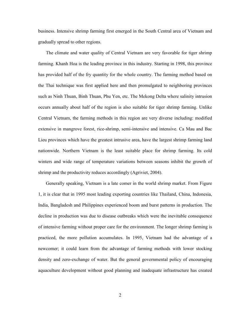
Generally speaking, Vietnam is a late comer in the world shrimp market. From Figure

1, it is clear that in 1995 most leading exporting countries like Thailand, China, Indonesia,

India, Bangladesh and Philippines experienced boom and burst patterns in production. The

decline in production was due to disease outbreaks which were the inevitable consequence

of intensive farming without proper care for the environment. The longer shrimp farming is

practiced, the more pollution accumulates. In 1995, Vietnam had the advantage of a

newcomer; it could learn from the advantage of farming methods with lower stocking

density and zero-exchange of water. But the general governmental policy of encouraging

aquaculture development without good planning and inadequate infrastructure has created

3

some problems. This haste reflected the hope of improving the standard of living by the

appealing profit from intensive shrimp farming which dominated the special attention to its

aftermath. In recent years, when intensive shrimp farming is widely practiced throughout

the country, both the government and farmers are starting to pay more attention to the effect

of the environment on shrimp yield.

Figure 1: Production in thousand tons of cultured shrimp in leading Asian countries (Primavera, 1997).

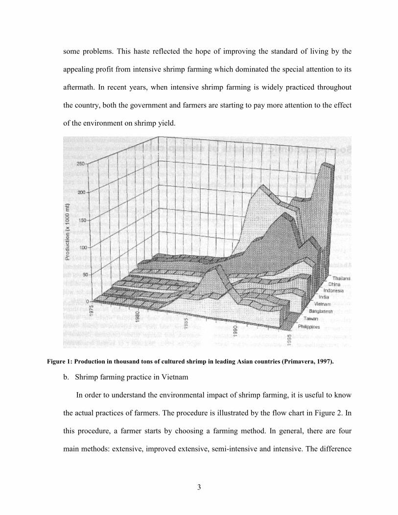
b. Shrimp farming practice in Vietnam

In order to understand the environmental impact of shrimp farming, it is useful to know

the actual practices of farmers. The procedure is illustrated by the flow chart in Figure 2. In

this procedure, a farmer starts by choosing a farming method. In general, there are four

main methods: extensive, improved extensive, semi-intensive and intensive. The difference

4

of these methods can be determined based on stocking density, use of aeration, shrimp yield

and level of management and capital investment. Farming method classification is

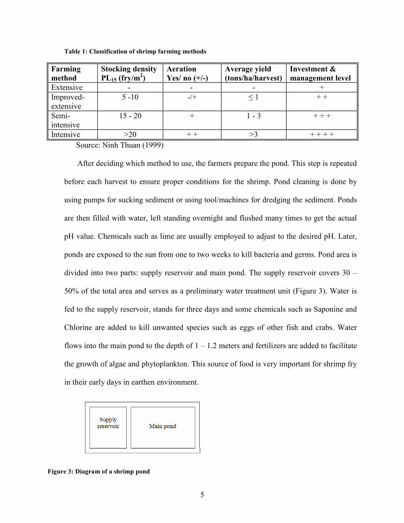
summarized in table 1 below (Ninh Thuan, 1999).

Figure 2: A brief procedure of shrimp farming

• Extensive farming makes use of large land area, natural stock and natural feed.

Today, most farmers supply more fry with low stock density but they still depend

totally on natural feed. This method is mainly applied in Ca Mau Province, Mekong

Delta.

• Improved extensive farming is very popular in the Mekong Delta and the Northern

Vietnam. Shrimp can be cultivated as a mono crop or rotated with rice or salt.

• Semi-intensive and intensive methods require higher stock density, aeration,

advanced level of management and investment so they produce higher yield. These

methods are applied in most areas of Vietnam.

5

Table 1: Classification of shrimp farming methods

Farming

method

Stocking density

PL15 (fry/m2)

Aeration

Yes/ no (+/-)

Average yield

(tons/ha/harvest)

Investment &

management level

Extensive - - - + Improved-extensive

5 -10 -/+ ≤ 1 + +

Semi-intensive

15 - 20 + 1 - 3 + + +

Intensive >20 + + >3 + + + + Source: Ninh Thuan (1999)

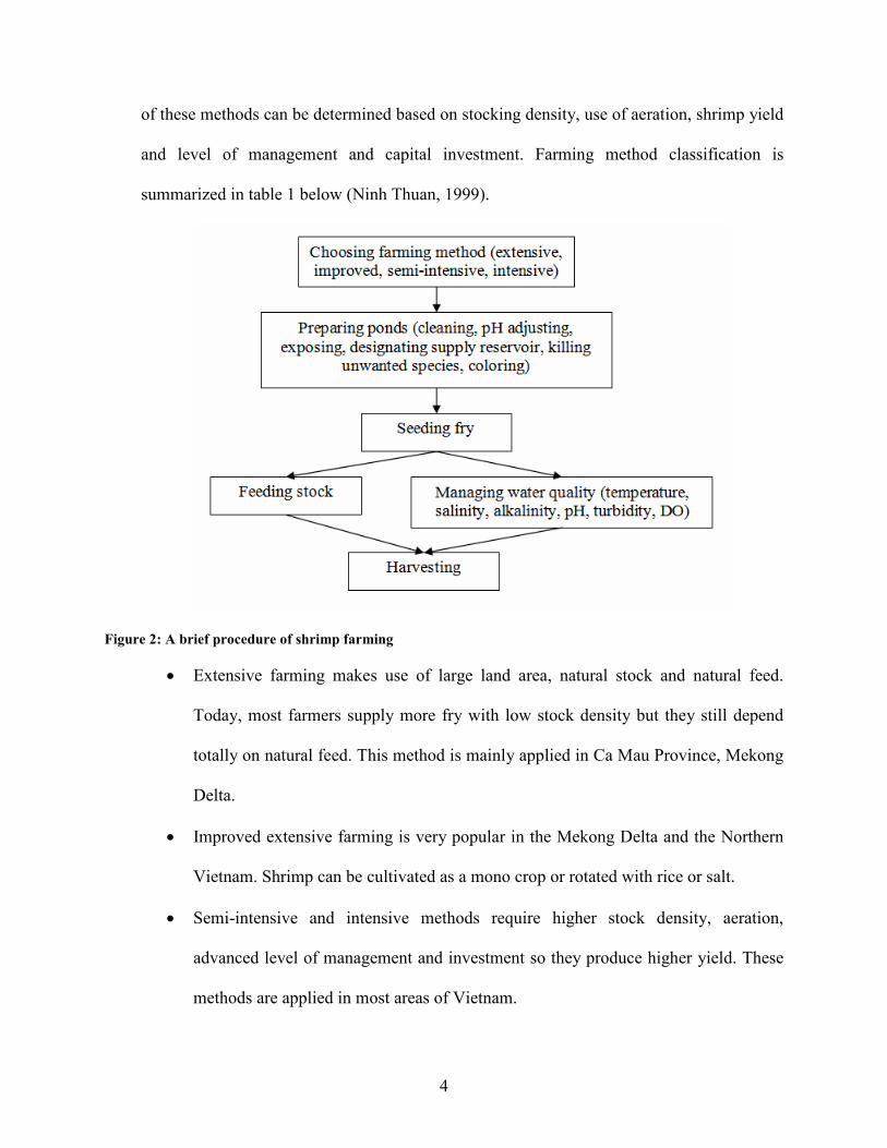
After deciding which method to use, the farmers prepare the pond. This step is repeated

before each harvest to ensure proper conditions for the shrimp. Pond cleaning is done by

using pumps for sucking sediment or using tool/machines for dredging the sediment. Ponds

are then filled with water, left standing overnight and flushed many times to get the actual

pH value. Chemicals such as lime are usually employed to adjust to the desired pH. Later,

ponds are exposed to the sun from one to two weeks to kill bacteria and germs. Pond area is

divided into two parts: supply reservoir and main pond. The supply reservoir covers 30 –

50% of the total area and serves as a preliminary water treatment unit (Figure 3). Water is

fed to the supply reservoir, stands for three days and some chemicals such as Saponine and

Chlorine are added to kill unwanted species such as eggs of other fish and crabs. Water

flows into the main pond to the depth of 1 – 1.2 meters and fertilizers are added to facilitate

the growth of algae and phytoplankton. This source of food is very important for shrimp fry

in their early days in earthen environment.

Figure 3: Diagram of a shrimp pond

6

When the ponds are ready, shrimp fry are cultured with varied density depending on the

method chosen. In intensive method, stock density usually ranges from 25 – 45 fry/m2.

Besides natural feed in the pond, home-made or industrial feed is also applied. At the same

time, water quality is monitored closely in terms of temperature, salinity, pH, turbidity,

dissolved oxygen (DO) and toxins (NH3, H2S, NO3, heavy metals, etc.). During this period,

shrimp might become diseased due to climatic factors or infection of viral diseases.

Farmers, therefore, have to apply antibiotics to keep the shrimp healthy. After 3.5 – 4.5

months, the shrimp are ready for harvest.

c. Environmental and socio-economic impacts of shrimp farming

In Vietnam, most farmers practice zero-exchange method which means that during a

harvest, no water is exchanged with the environment. This method helps reduce nutrient

loss and maintain acceptable water quality (Thakur & Lin, 2003). However, throughout the

farming procedure, many chemicals and nutrients are intentionally added to the pond.

Chemical pollution affects and kills non-targeted species. These chemicals are very

persistent so their impact is unpredictable. Nutrient pollution causes eutrophication in the

channel systems and waterways. Viruses from shrimp ponds and dead shrimp without

proper treatment in a nutrient-rich environment enhance the growth of water-borne

diseases. In turn, these impacts decreases shrimp yield and cause the farming system to fail

after a period of time.

The environmental impacts of shrimp farming are even more serious in areas near

mangrove forests, coral reefs and sea grasses, Melaleuca forests and freshwater wetlands

(Environmental Justice Foundation, 2003). Biodiversity loss of these ecosystems is the

main cause leading to system malfunctioning. This phenomenon adds more severity to

7

natural disasters in these regions. Furthermore, shrimp farming also induces groundwater

and soil salinization.

Resource use conflict, mainly water use, happens between farmers growing cash crops

such as rice or sugarcane and shrimp farming farmers. Oftentimes, people share the same

channel system and the effluent from shrimp farms with high salinity reduces the yield of

rice/sugarcane crops significantly. This seems to be not very serious because the fraction of

rice or sugarcane area in shrimp farming regions is relatively small compared to shrimp

farms.

The profit from intensive shrimp farming is more than 30-fold greater than profit from

rice farming. A harvest is considered successful when both yield and price are high. With a

successful harvest, farmers can earn tens of thousand of dollars per hectare. This profit

enables them to repay loans, reinvest in the next harvest and improve their standard of

living. In contrast, an unsuccessful harvest traps them in the spiral of debt due to high

investment. From a research of assessing poverty in Tra Vinh province in the Mekong

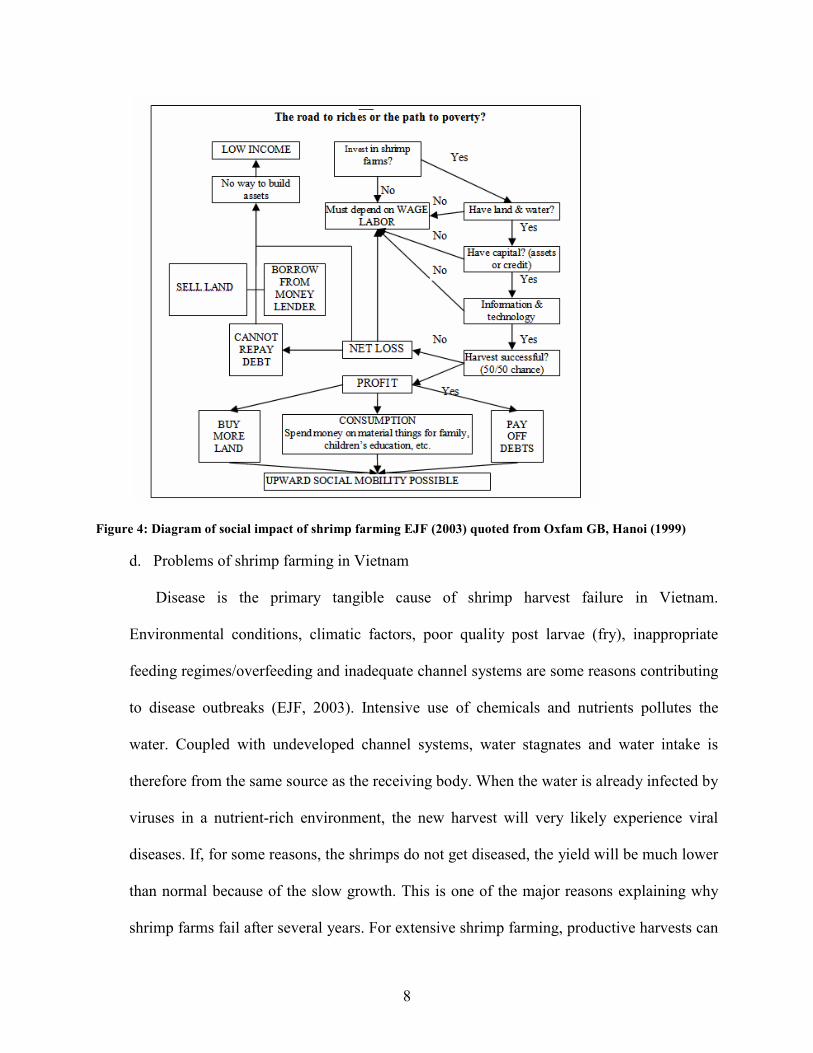
Delta, Oxfam Great Britain modeled the socio-economic impact as shown in Figure 4. Most

farmers abandon their land after several failed harvests. Some of them rent or sell their land

and work for others but this does not improve their situation. Adding more risk into this

business is the habit of most farmers of not building a saving account.

8

Figure 4: Diagram of social impact of shrimp farming EJF (2003) quoted from Oxfam GB, Hanoi (1999)

d. Problems of shrimp farming in Vietnam

Disease is the primary tangible cause of shrimp harvest failure in Vietnam.

Environmental conditions, climatic factors, poor quality post larvae (fry), inappropriate

feeding regimes/overfeeding and inadequate channel systems are some reasons contributing

to disease outbreaks (EJF, 2003). Intensive use of chemicals and nutrients pollutes the

water. Coupled with undeveloped channel systems, water stagnates and water intake is

therefore from the same source as the receiving body. When the water is already infected by

viruses in a nutrient-rich environment, the new harvest will very likely experience viral

diseases. If, for some reasons, the shrimps do not get diseased, the yield will be much lower

than normal because of the slow growth. This is one of the major reasons explaining why

shrimp farms fail after several years. For extensive shrimp farming, productive harvests can

9

last for 10 – 20 years. The semi-intensive method only works for about 5 – 10 years and

intensive systems fail after 5 years (EJF, 2003).

Shrimp are quite sensitive to temperature changes and Vietnam is a tropical country

with two distinct seasons. Temperatures vary from 10 – 120C between dry and rainy

seasons whereas a variation of 5 – 60C can cause shrimp to die.

Post larvae quality is also a big concern because not all regions can produce fry locally.

Traveling long distant induces stress for young shrimp. Farmers often use their naked eye to

test fry quality which is often misleading due to the hatchery’s use of antibiotics. Only

some farmers send the fry to be tested. As a result, for the most part, farmers are not

provided with good quality fry.

The feeding regime is another important aspect in shrimp farming. Shrimp should be

caught and weighed every 7 – 10 days to determine survival rates and body weight. Based

on these parameters, the amount of feed is calculated accordingly. Feeding must follow a

strict schedule. Poor farmers feed their shrimp poorly when they have little money and feed

shrimp excessively when they have enough money. Some always overfeed their shrimps

hoping to get higher yield. These inappropriate practices cause the shrimp to be unhealthy

and greatly reduce the yield.

Shrimp production is known by many farmers as a profitable and risky business. High

levels of investment require high reinvestment because most costs lie in feed cost and other

operating costs. Unsuccessful farmers abandon their farms because converting back to rice

is difficult. It is difficult in a sense that farmers have to invest to transform the deep pond

into the shallower field. Shrimp ponds have accumulated high levels of salinity so they

need to be flushed many times before growing rice. As a result, the first few crops of rice

10

will have a very low yield. Shrimp production is also risky because fry and feed quality

provided by separate sellers is unknown although this is not always the case in every

region. The marketing channel is mainly driven by collectors or middlemen who have some

power to influence the price because most shrimp farms are in the coastal zone far away

from the main market. Figure 5 illustrates a marketing channel in Phu Tan in Mekong Delta

(EJF quoted from Nguyen Van Be). This structure reveals the monopsony power of

middlemen or collectors in the market. In order to maximize their net benefit from

purchasing shrimp, they purchase a smaller quantity at a lower price compared to that of the

competitive market. As a result, monopsony makes the buyers better off and the sellers

worse off. The resulting deadweight loss is the source of inefficiency if there is no market

failure due to some sources of externalities.

The government has a regulation specifying when to grow shrimp and how to treat

infected dead shrimp. However, regulation violation occurs in several places. People tend to

grow two harvests per year instead of one which is the recommended level of the

government and do not treat the dead shrimp thoroughly. The second harvest often

produces a lower yield and has a greater chance for the shrimp to be infected. These two

practices cause the farming system to fail more quickly.

Figure 5: Shrimp marketing channel in Phu Tan (EJF (2003) cited from Nguyen Van Be (2000))

11

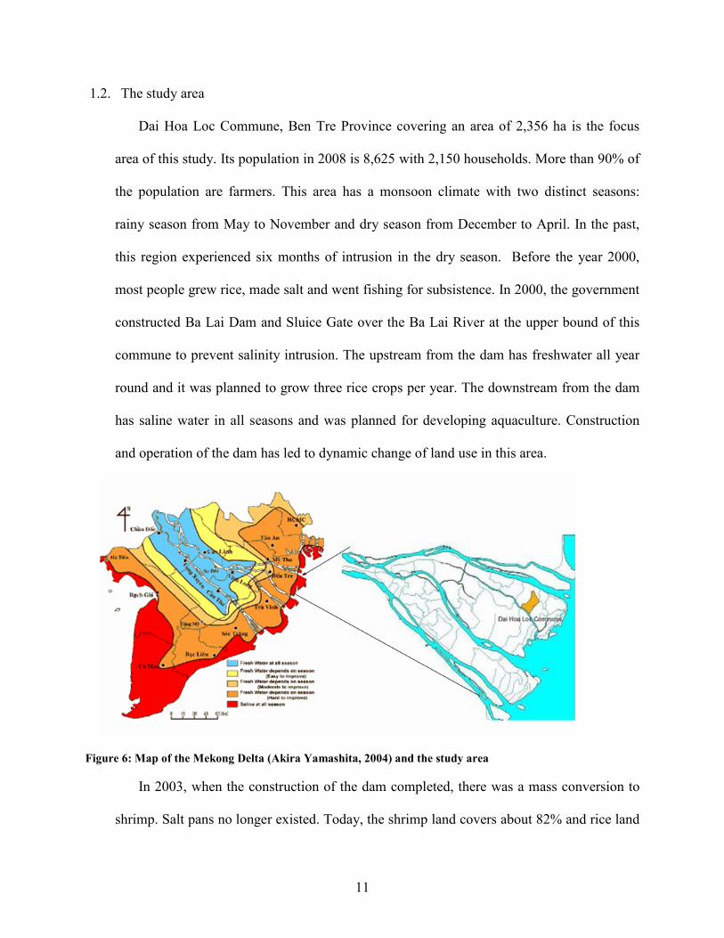
1.2. The study area

Dai Hoa Loc Commune, Ben Tre Province covering an area of 2,356 ha is the focus

area of this study. Its population in 2008 is 8,625 with 2,150 households. More than 90% of

the population are farmers. This area has a monsoon climate with two distinct seasons:

rainy season from May to November and dry season from December to April. In the past,

this region experienced six months of intrusion in the dry season. Before the year 2000,

most people grew rice, made salt and went fishing for subsistence. In 2000, the government

constructed Ba Lai Dam and Sluice Gate over the Ba Lai River at the upper bound of this

commune to prevent salinity intrusion. The upstream from the dam has freshwater all year

round and it was planned to grow three rice crops per year. The downstream from the dam

has saline water in all seasons and was planned for developing aquaculture. Construction

and operation of the dam has led to dynamic change of land use in this area.

Figure 6: Map of the Mekong Delta (Akira Yamashita, 2004) and the study area

In 2003, when the construction of the dam completed, there was a mass conversion to

shrimp. Salt pans no longer existed. Today, the shrimp land covers about 82% and rice land

12

covers 10% of the total arable land. Following is the land statistics from 2005 – 2007

(Table 2) and population data from 2006 to 2008 (Table 3).

Table 2: Land use in Dai Hoa Loc from 2005 to 2007 (People’s Committee of Dai Hoa Loc, personal

communication, 2008)

Year Land category

2005 2006 2007

Arable land (ha) 2,055 2,057 2,057 Aquaculture (ha) 1,677 1,679 1,694 Rice (ha) 233 233 217 Total land 2,356 2,356 2,356

Table 3: Population of Dai Hoa Loc from 2006 to 2008 (People’s Committee of Dai Hoa Loc, personal

communication, 2008)

2006 2007 2008

Male 3634 3658 4307 Female 4443 4462 4318 Total 8077 8120 8625 Growth rate 0.027 0.005 0.062

1.3. Objectives of the study

The focus of this paper is the driving force of land use change, the effect of shrimp

farming practice on the environment and how that influences shrimp yield in return. Farmers

in this region observed the profit per ha from pilot shrimp farms then they compared with the

profit per ha from rice and decided to change. It takes people some years to realize the profit

and learn the new farming technique. When more farmers are capable of shrimp technique,

they shift to shrimp faster. Under the monopsony power of the market, the price of shrimp

decreases due to the large amount of supply, and the profit per ha of land decreases. On the

other hand, the more shrimp land grows, the more nitrogen is discharged into the

environment in the form of sediment and drainage water. Some of the nitrogen content is

transported by tide, and the rest stays in the channel system. Because the water supply

channel is also the receiving body, nitrogen remaining in the channel finds its way to the

13

shrimp pond. High nitrogen content in the pond at subsequent harvest reduces shrimp yield.

Farmers evaluate the risk of shrimp by counting the years they earn low profit. Several years

of low profit retard the conversion process. All of these complex interactions will be

represented in a simulation model.

Sensitivity analysis of the model will show how different stocking density affects shrimp

yield and channel pollution. The model will also be used to show how the borrowing period

and the tidal removal rate affect the conversion process. The main purpose of the model is

policy testing. Policy tests include stock density reduction, the introduction of treatment

ponds and the investment to improve the channel system. The cost of these policies is

compared with the benefit of reducing nitrogen content in the channel system to see if

sustainability would be obtained.

14

CHAPTER TWO

METHODOLOGY

2.1. System Dynamics:

System Dynamics is a method of analyzing problems over time to help understand

system components’ interaction and the interplay between the system and the environment

(Coyle, 1977). This methodology was first developed in the 1960s by Jay Forrester. It is very

useful in revealing complex feedback loops within the system, and this knowledge helps

improve the system’s performance.

In this paper, Stella 9.1 is used to model the system and conduct numerical simulations.

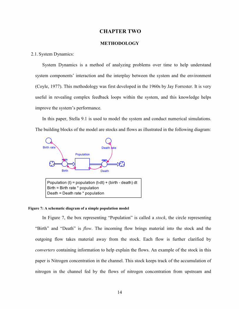
The building blocks of the model are stocks and flows as illustrated in the following diagram:

Population

Birth Death

Birth rate Death rate

Population (t) = population (t-dt) + (birth - death) dt

Birth = Birth rate * population

Death = Death rate * population

Figure 7: A schematic diagram of a simple population model

In Figure 7, the box representing “Population” is called a stock, the circle representing

“Birth” and “Death” is flow. The incoming flow brings material into the stock and the

outgoing flow takes material away from the stock. Each flow is further clarified by

converters containing information to help explain the flows. An example of the stock in this

paper is Nitrogen concentration in the channel. This stock keeps track of the accumulation of

nitrogen in the channel fed by the flows of nitrogen concentration from upstream and

15

nitrogen concentration in the drainage water, and the flow of the tide removing the nitrogen

out of this stock.

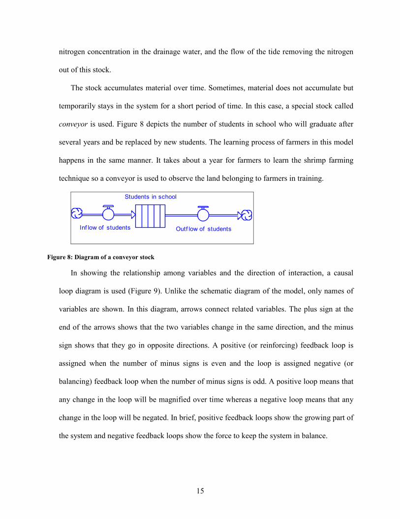
The stock accumulates material over time. Sometimes, material does not accumulate but

temporarily stays in the system for a short period of time. In this case, a special stock called

conveyor is used. Figure 8 depicts the number of students in school who will graduate after

several years and be replaced by new students. The learning process of farmers in this model

happens in the same manner. It takes about a year for farmers to learn the shrimp farming

technique so a conveyor is used to observe the land belonging to farmers in training.

Students in school

Inf low of students Outf low of students

Figure 8: Diagram of a conveyor stock

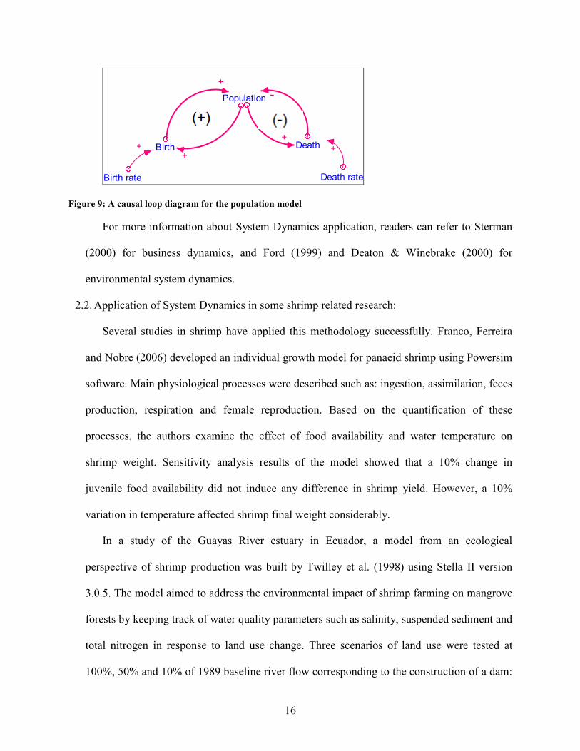
In showing the relationship among variables and the direction of interaction, a causal

loop diagram is used (Figure 9). Unlike the schematic diagram of the model, only names of

variables are shown. In this diagram, arrows connect related variables. The plus sign at the

end of the arrows shows that the two variables change in the same direction, and the minus

sign shows that they go in opposite directions. A positive (or reinforcing) feedback loop is

assigned when the number of minus signs is even and the loop is assigned negative (or

balancing) feedback loop when the number of minus signs is odd. A positive loop means that

any change in the loop will be magnified over time whereas a negative loop means that any

change in the loop will be negated. In brief, positive feedback loops show the growing part of

the system and negative feedback loops show the force to keep the system in balance.

16

Population

Birth Death

Birth rate Death rate

+

+

-

++ +

Figure 9: A causal loop diagram for the population model

For more information about System Dynamics application, readers can refer to Sterman

(2000) for business dynamics, and Ford (1999) and Deaton & Winebrake (2000) for

environmental system dynamics.

2.2. Application of System Dynamics in some shrimp related research:

Several studies in shrimp have applied this methodology successfully. Franco, Ferreira

and Nobre (2006) developed an individual growth model for panaeid shrimp using Powersim

software. Main physiological processes were described such as: ingestion, assimilation, feces

production, respiration and female reproduction. Based on the quantification of these

processes, the authors examine the effect of food availability and water temperature on

shrimp weight. Sensitivity analysis results of the model showed that a 10% change in

juvenile food availability did not induce any difference in shrimp yield. However, a 10%

variation in temperature affected shrimp final weight considerably.

In a study of the Guayas River estuary in Ecuador, a model from an ecological

perspective of shrimp production was built by Twilley et al. (1998) using Stella II version

3.0.5. The model aimed to address the environmental impact of shrimp farming on mangrove

forests by keeping track of water quality parameters such as salinity, suspended sediment and

total nitrogen in response to land use change. Three scenarios of land use were tested at

100%, 50% and 10% of 1989 baseline river flow corresponding to the construction of a dam:

17

(1) 100% mangrove, (2) 50% mangrove and 50% shrimp pond and (3) 100% shrimp pond.

Water quality remained good due to the low residence time in the estuary because of high

water flow and tidal exchange rate. However, with a 90% reduction in mangrove forest due

to converting to shrimp pond, total nitrogen concentration increased five times. Nitrogen

concentration even became 60 times higher if river discharge decreased to 10%. The

topography and hydrograph of the estuary also influenced water quality as nitrogen

concentration of the upper estuary region increased more quickly while it did not change

much in the lower region. The authors believed that the integration of this model into

economic analysis would better evaluate the economic impacts of coastal zone management

policy.

In line with studying the impact of shrimp farming on mangrove forests, Arquitt,

Honggang and Johnstone (2005) developed a model for the case of Thailand, one of the

world’s largest shrimp production countries. The model tried to shed light on the interaction

among market demand, shrimp production and the environment by constructing inventory,

production and ecology sectors. Simulating the model for 50 years with a time step of 0.125

years showed the overshoot pattern of Total Thai Production, Thai Mangrove Farm

Production and Thai Inland Coastal Farm Production. This pattern happened as a result of

over-investment in shrimp farming when the demand was high which caused tremendous

mangrove forest loss. Three policies of Technology, Eco-taxes and Export Tax with Rebate

were considered to test if it is possible to maintain the benefit from shrimp while preserving

the mangrove forests. The Export Tax with Rebate turned out to be the best. The idea of this

policy is to tax each unit of exported shrimp and rebate to farmers certified with sustainable

practice. Three tax levels of $1, $2 and $3 per kg were applied for the sensitivity test. Results

18

showed that the overshoot pattern started to decrease at the tax level of $2 and gradually

shifted toward a sustainable pattern at the level of $3. Combining the tax of $3 and

technological improvement indicated a sustainable trend of Thai production and Mangrove

Farm. The production rate in this case was higher than the rebate fee alone. Coupled with the

rebate fee, this policy enabled farmers to restrict themselves in developing new farms on

susceptible areas. However, for the case of Thailand, this policy did not work well as Thai

mangrove was highly degraded at the time of the research. The authors would like to

consider this policy as a learning experience which should apply for unexploited mangroves

in Asia, Africa and Latin American.

For the context of intensive shrimp farming in Ninh Thuan –Vietnam, Soo (2005) built a

model revealing the development of shrimp farms and its effect on land price, revenues, and

ground water quantity and pond water quality. The propagation of shrimp farms was based

on the performance of first generation farms in 1999. The more pilot farms performed well,

the more attractive shrimp production became. This attractiveness increased land prices

which in turn reduced the rate of converting to shrimp ponds. The increase in shrimp farms

also led to an increase in nitrogen and phosphorous sediment in ponds and a decrease in

groundwater storage. Coupled with high stocking density, high sediment load worsened pond

water quality which affected shrimp survival and yield. The groundwater quantity was

calculated based on precipitation and used to test if it was one of the limiting factors to

shrimp farming. Results showed that with a stocking density of 40 fry/m2 and no cleaning

action, the life time of the shrimp pond was 19 seasons. From a starting area of 50 ha, after

12 seasons, 317 ha of land was converted to shrimp farms. Reducing stocking density from

40 to 15 fry/m2 in the 15th season would extend the system performance for 10 more years.

19

Keeping the stock density at 40 fry/m2 and cleaning the pond in the 15th season with 20%

removal efficiency, 1624 ha of land was converted to ponds within 52 seasons. In this

scenario, groundwater storage declined tremendously and was depleted in the 52nd season

which closed down the business. Increasing the cleaning efficiency to 40% in 15th season,

within 48 seasons, 1518 ha of land was converted. Groundwater became the limiting factor in

the 48th season. Combining the low stock of 15 fry/m2 and cleaning activity of 40%

efficiency, the groundwater problem occurred in the 70th season and 1294 ha of land was

converted.

Although the four studies in shrimp cover different scales and aspects of this industry,

they have some common features: researching complex dynamics, containing a lot of

uncertainties and providing practical simulation analysis. In an effort to apply the same

methodology to shrimp farming in Dai Hoa Loc Commune, this paper will be based heavily

on some concepts in the paper by Soo (2005).

20

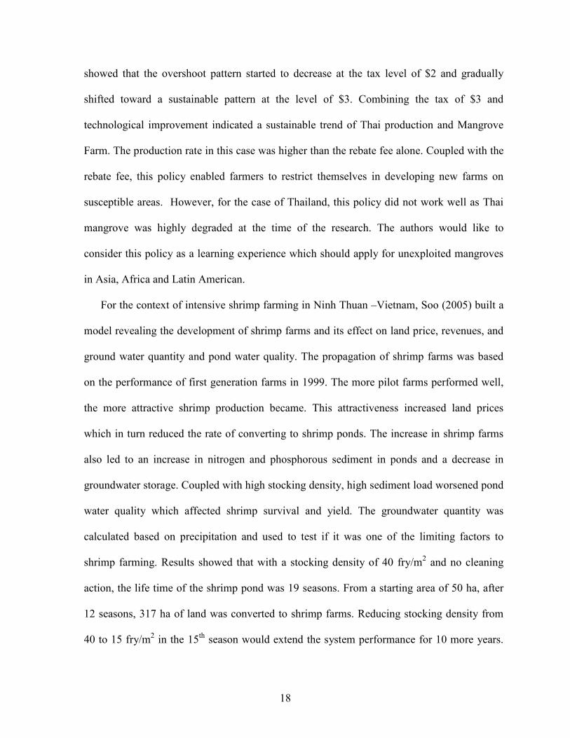
CHAPTER THREE

THE MODEL

3.1 Model structure and description:

The model includes two modules: Shrimp land and Nitrogen. The interaction between

these modules can be described as follows. When more shrimp land is developed, more

nitrogen is discharged into the environment. The nitrogen will deteriorate water quality,

reduce shrimp yield and shrimp profit, and slow down the development of shrimp land. This

is a typical pattern of development reaching the carrying capacity of the environment. As

mentioned in the introduction chapter, farmers tend to do two harvests per year. However, for

simplicity, in this model we count only one harvest a year.

Rice land Pilot shrimp f arm

~

Pilot project creation

Mass conv ersion

First y ear shrimp f arm

Pilot f arm with results

proceeding to harv est

Old shrimp f arm

aging

Land with f armers rice capable

Land with f armers rice

and shrimp capable

Land with f armers in training

initiate training

complete training

Figure 10: Stock and flow diagram of Shrimp land module

The Shrimp land module describes the conversion process from rice land to shrimp land.

The process begins when some pilot farms are created. People observe the profit from these

farms, compare with the profit from rice and start being interested in shrimp farming. In this

21

model, rice price is fixed for easier comparison. It takes the farmers a while to observe the

profit and this is represented by the lag time in observing. When the high profit of shrimp

farming becomes well-known, rice farmers begin to learn the new farming technology. It

takes them about one year to take training courses and learn from neighbors. At the same

time of observing profit, they also count the bad years when there is no net benefit or even is

a net loss. After gaining the necessary technique and lessons, they make the decision to

convert to shrimp, the mass conversion process in Figure 10. The separation of first year

shrimp farms from old farms serves for cost calculation purpose only. In the first year, the

investment is higher than subsequent years due to the fixed cost of preparing/creating the

pond. To most farmers, this cost is calculated once and this explains why the profit from the

first year is not very high. There are additional operating costs such as labor cost, equipment

operation cost, seed and feed costs. Seed and feed costs are dependent on the stocking

density. In addition, most farmers borrow money from the bank and they have to pay off the

debt. The typical borrowing period ranges from 1 – 5 years. The revenue from shrimp is

computed based on the shrimp yield and shrimp price which is driven by the monopsony

market. In calculating the shrimp supply, only effective land is taken into account. Effective

land is the actual area of the main pond without the supply reservoir. The annual average

income from both rice and shrimp is also tracked to see if the community is better off or

worse off when shifting to shrimp. There are four variables of this module connecting to the

next module: stock density, feed applied, shrimp yield and total effective shrimp land. The

full diagram of this module is in figure 11.

22


~


Mass conv ersion




and shrimp capable


Rice y ield

Rice unit operating cost

Rice price

Rice prof it per ha

First year shrimp profit

initial land area

Rice rev enue

initial land area



total shrimp supply

Shrimp unit f ixed cost

Shrimp unit operating cost

Nitrogen.shrimp yield

Shrimp rev enue per ha

Old f arm shrimp prof it per ha

loan interest rate

+

Total 1 year f arm

~

Shrimp price

annual payment

inital loan

First y ear shrimp prof it

Total 1 y ear

ef f ectiv e land

Shrimp prof it ratio

Ev idence of prof it

Observ ed shrimp prof it ratio

lag time~

f raction of f armers

interested in shrimp f arming

initiate training

f raction of rice land

conv erted per y r

~


adopting change

Total ef f ectiv e old shrimp land

Number of bad y ears

Old shrimp f arm

aging

Nitrogen.Shrimp?

First y ear shrimp rev enue

counting

+

Total old shrimp land

Start?

Supply reserv oir

area f raction

Prof it f rom shrimp


Old farm shrimp profit per ha

total prof it

Total effective old shrimp land

Rice profit per ha

Rice land

Total 1 year

effective land

+

Total ef f ectiv e shrimp land

borrowing period

complete training

First y ear f arm existence

Old shrimp f arm existence

Population

Growth

growth rate

annual av erage income

Feed and seed cost

Feed cost Seed cost

Nitrogen.Stock density

Fry unit priceNitrogen.Feed applied

Feed unit cost

Feed and seed cost

Old farm shrimp profit per ha

Figure 11: Full diagram of the Shrimp land module

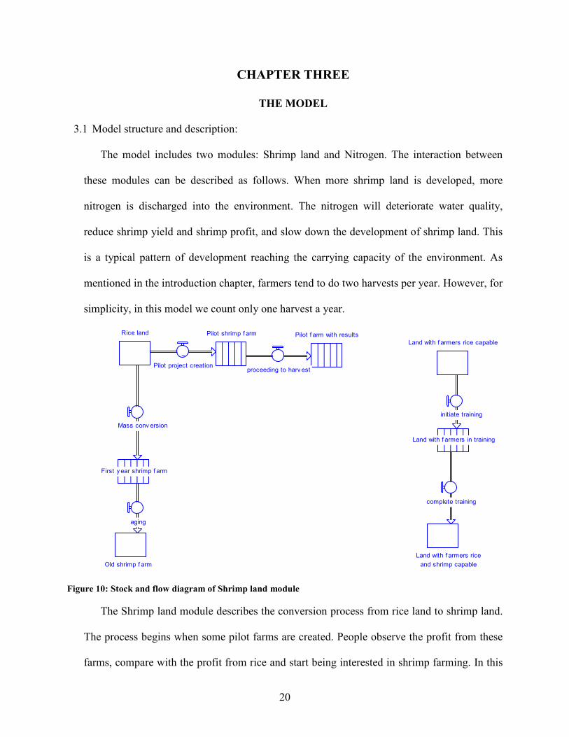
The Nitrogen module keeps track of Nitrogen of both the water and sediment phase from

the pond to the channel system (Figure 12). The source of Nitrogen includes fertilizer, seed,

intake water and feed. While fertilizer is a fixed amount for each ha of the shrimp pond, feed

is dependent on the stock density. The amount of feed applied is calculated based on an

average feeding scheme. Most nitrogen ends up in the pond sediment in the form of dead

shrimp, feces, excess feed, plankton and bacteria. The remaining nitrogen is in the harvested

shrimp, removed by drainage water when harvested or lost in the form of gases such as NH3,

N2 or N2O. About 90% of the sediment is dredged out of the pond after harvest and

discharged into the channel.

23

Figure 12: Stock and flow diagram of Nitrogen module

A small fraction of nitrogen in pond sediment goes back to the water phase during the

remineralization process. Once the nitrogen makes its way to the channel, two main

processes take place: biodegradation and tidal removal. In this region, the tidal pattern is

semi-diurnal which means there are two high tides and two low tides each day. Due to the

frequent and continual tidal action, tidal removal is more important than biodegradation. As a

result, only the tidal effect is taken into account in the model. The nitrogen in the channel is

supplemented by the agricultural and domestic water use upstream. The intake water is

withdrawn from the channel. In this module, the nitrogen is calculated based on one ha of

shrimp land (main pond area) so the total pollution is multiplied by Total effective shrimp

land. The water flow demand is the water volume that should be maintained during shrimp

24

farming in each ha of main pond. The typical value for water level ranges from 1 – 1.5 m so

we take the average value of 1.2 m for calculation. This means that for one ha of main pond,

there should be 12,000 m3 water. In addition to keeping track of nitrogen, shrimp survival is

also observed. Shrimp survival rate depends on not only the stock density but also other

environmental factors. Making use of the information of ammonia toxicity, we consider the

nitrogen concentration in the shrimp pond as the limiting factor to shrimp growth. In reality,

farmers may use aerators or chemicals to control pH and thereby adjust ammonia

concentration, hence the effect of ammonia is not serious. However, because viruses and

other physical parameters are random and hard to keep track of, this is a much simpler way to

account for the environmental impact. The full diagram of this module is shown in Figure 13.

N in the pond

N concentration in the channel

N of intake water

N f rom f eed

N f rom seed and f ertilizer

Volatization

N in shrimp

Sedimentation

N in channel sediment

Stock density

Feed applied

Percent of N in f eed

~

f eed by density

N conc in intake water

N removed by drainage

to the channel

N removal drainage rateremineralization

~

sediment removal rate

Removal by tide

Treatment ef f iciency

of supply reserv oir

annual water flow demand per ha

Fry weight

N in f ry

Fertilizer

annual water f low demand per ha

Shrimp land.Start?

Total N discharge mass

N in pond sediment

~

shrimp surv iv al rate by density

dredging removal rate

~

Shrimp surv iv al rate by N ef f ect

~

sedimination rate

~

drain water sedimentation ratio

Volatization f raction

N in the pond

N concentration in pond

Number of surv iv al shrimp

integrated surv iv al rate

Shrimp land.Start?

expected shrimp weight

shrimp y ield

percent of dry weight

Shrimp dry weight

percent of N in shrimp weight

Stock density

dredgingannual water flow demand per ha

Shrimp?

Tidal removal

Shrimp dry weight


remineralization rate

~

tidal removal rate

N concentration

f rom drainage water

Stock density

~

Shrimp land.Total effective

shrimp land

Channel estimated v olume

N concentration

f rom upstream

total discharge v olume

~

shrimp survival rate by density

discharge sediment

Figure 13: Full diagram of the Nitrogen module

25

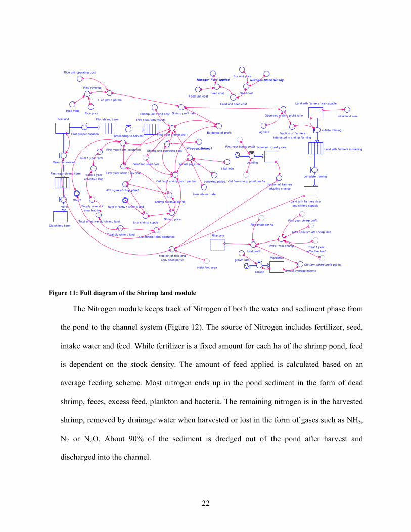
3.2 Causal loop diagram

From a farmer’s perspective, the Profit responding loop is the most easily seen (Figure

14). This is a negative loop in the Shrimp land module. When there are more shrimp farms,

shrimp supply increases which causes the shrimp price to fall. Accordingly, shrimp profit

decreases which influences the shrimp profit ratio. After a lag time, people observe the fall in

the shrimp profit ratio and the fraction of farmers interested in shrimp farming declines.

There are fewer people attending training courses and becoming capable of both rice and

shrimp farming. The fraction of rice land converted annually will drop. There would be less

land conversion from rice to shrimp.

Shrimp y ieldShrimp land

Shrimp supply

Shrimp price

Shrimp prof it

Fraction of f armers



and shrimp capable

Fraction of rice land

converted per y ear

Mass conv ersion

Rice land


Shrimp cost

loan & f ixed cost & operating cost

+

+

-

+

-

+

+

+

-

+-

-

Figure 14: The Profit responding loop

The other three main loops in the Nitrogen module (Figure 15) are harder to observe. The

first positive loop involves nitrogen cycling. When the concentration of nitrogen in intake

water is high, the nitrogen content in the pond is also high. The more water is drained into the

channel, the more nitrogen is discharged. Nitrogen ends up in the channel causing an increase

in nitrogen concentration of the intake water.

The second positive feedback loop involves sediment cycling in the pond. A large

amount of nitrogen in the pond enhances the sedimentation process and deposits more

26

nitrogen in the pond sediment. On the other hand, remineralization increases when nitrogen

content in the sediment gets higher and higher. This process adds more nitrogen content into

the water phase.

N in the pond

N remov ed by drainage

to the channel

N concentration

in the channel

Sediment removal rate

N concentration

in intake water

Remov al by tide

Tidal removal rate



Sedimentation N in pond sediment

Remineralization



N removed by shrimp growth

Shrimp y ield

+

+

+

-

+

-

+

-

+

-

+

+

++

-

+

+

+

-

-

Figure 15: Causal loop diagram of the Nitrogen Module

The third positive loop in the Nitrogen module involves nitrogen cycling by shrimp

growth. When the nitrogen content in the water phase of the pond is high, shrimp become

poisoned and reduce their population. Accordingly, shrimp yield is low and the nitrogen

content removed by shrimp growth is low, leaving a large amount of nitrogen in the pond

water. The fact that this is a positive loop may cause some counterintuitive opinions.

However, the main interpretation of this loop is that adding more nitrogen into the pond does

not help increase the shrimp yield but increase the nitrogen in the water phase of the pond.

The key loop in the model joining the two modules together is the density control loop

(Figure 16). The dash line connecting Shrimp supply and the Stock density represents the

implicit link in the model by experimenting with the slider to change stock density. This key

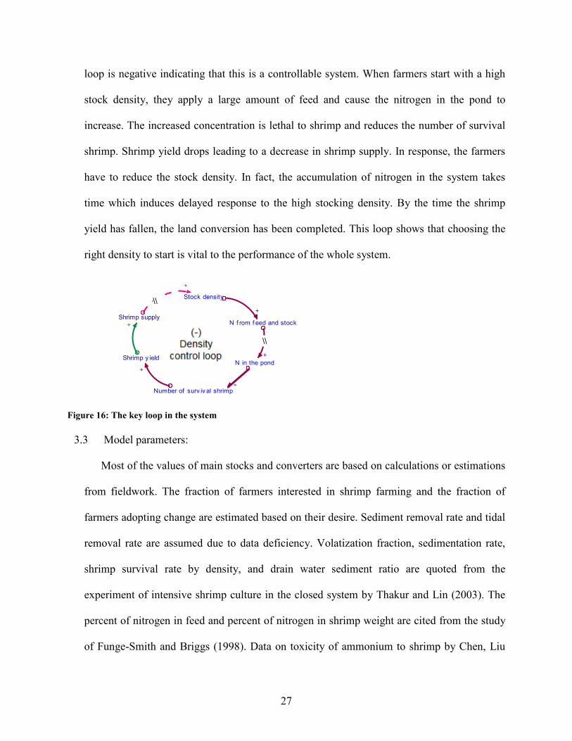
27

loop is negative indicating that this is a controllable system. When farmers start with a high

stock density, they apply a large amount of feed and cause the nitrogen in the pond to

increase. The increased concentration is lethal to shrimp and reduces the number of survival

shrimp. Shrimp yield drops leading to a decrease in shrimp supply. In response, the farmers

have to reduce the stock density. In fact, the accumulation of nitrogen in the system takes

time which induces delayed response to the high stocking density. By the time the shrimp

yield has fallen, the land conversion has been completed. This loop shows that choosing the

right density to start is vital to the performance of the whole system.

N in the pond


Stock density

Shrimp y ield

N f rom f eed and stockShrimp supply

+

+

+

+

-

+

\\

\\

Figure 16: The key loop in the system

3.3 Model parameters:

Most of the values of main stocks and converters are based on calculations or estimations

from fieldwork. The fraction of farmers interested in shrimp farming and the fraction of

farmers adopting change are estimated based on their desire. Sediment removal rate and tidal

removal rate are assumed due to data deficiency. Volatization fraction, sedimentation rate,

shrimp survival rate by density, and drain water sediment ratio are quoted from the

experiment of intensive shrimp culture in the closed system by Thakur and Lin (2003). The

percent of nitrogen in feed and percent of nitrogen in shrimp weight are cited from the study

of Funge-Smith and Briggs (1998). Data on toxicity of ammonium to shrimp by Chen, Liu

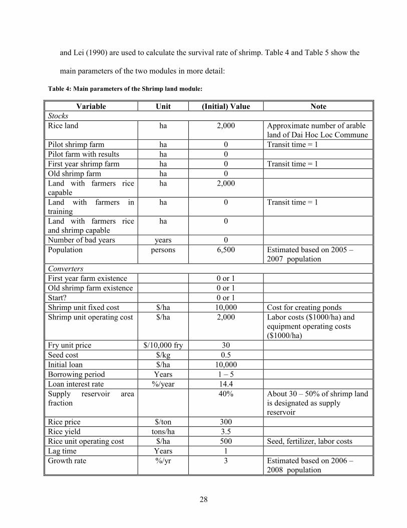
28

and Lei (1990) are used to calculate the survival rate of shrimp. Table 4 and Table 5 show the

main parameters of the two modules in more detail:

Table 4: Main parameters of the Shrimp land module:

Variable Unit (Initial) Value Note

Stocks Rice land ha 2,000 Approximate number of arable

land of Dai Hoc Loc Commune Pilot shrimp farm ha 0 Transit time = 1 Pilot farm with results ha 0 First year shrimp farm ha 0 Transit time = 1 Old shrimp farm ha 0 Land with farmers rice capable

ha 2,000

Land with farmers in training

ha 0 Transit time = 1

Land with farmers rice and shrimp capable

ha 0

Number of bad years years 0 Population persons 6,500 Estimated based on 2005 –

2007 population Converters First year farm existence 0 or 1 Old shrimp farm existence 0 or 1 Start? 0 or 1 Shrimp unit fixed cost $/ha 10,000 Cost for creating ponds Shrimp unit operating cost $/ha 2,000 Labor costs ($1000/ha) and

equipment operating costs ($1000/ha)

Fry unit price $/10,000 fry 30 Seed cost $/kg 0.5 Initial loan $/ha 10,000 Borrowing period Years 1 – 5 Loan interest rate %/year 14.4 Supply reservoir area fraction

40% About 30 – 50% of shrimp land is designated as supply reservoir

Rice price $/ton 300 Rice yield tons/ha 3.5 Rice unit operating cost $/ha 500 Seed, fertilizer, labor costs Lag time Years 1 Growth rate %/yr 3 Estimated based on 2006 –

2008 population

29

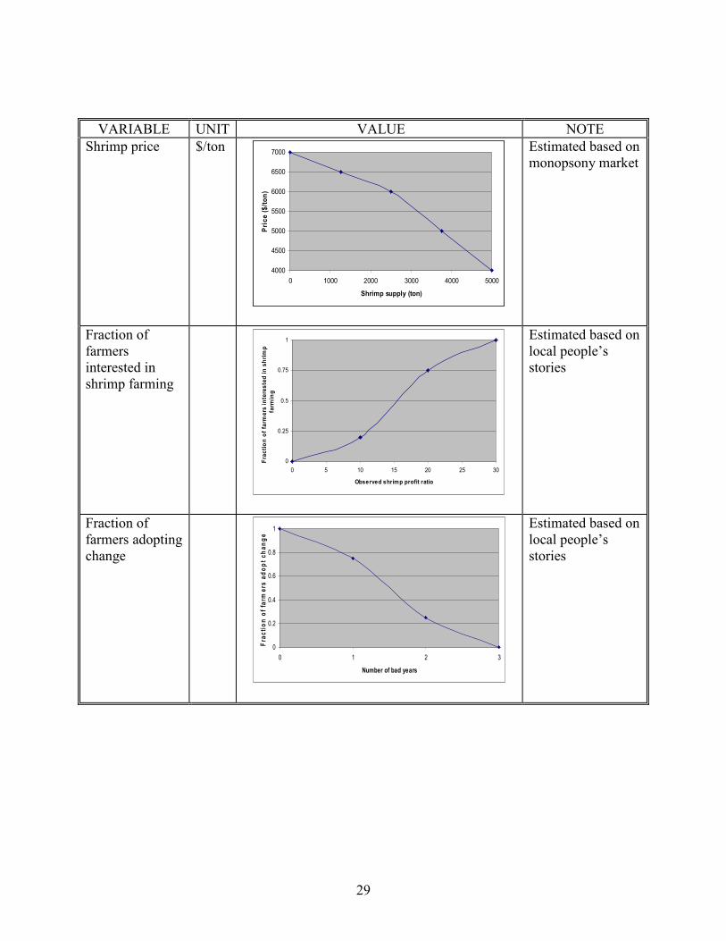
VARIABLE UNIT VALUE NOTE Shrimp price $/ton

4000

4500

5000

5500

6000

6500

7000

0 1000 2000 3000 4000 5000

Shrimp supply (ton)

Price ($/ton)

Estimated based on monopsony market

Fraction of farmers interested in shrimp farming

0

0.25

0.5

0.75

1

0 5 10 15 20 25 30

Observed shrimp profit ratio

Fraction of farm

ers interested in shrimp

farm

ing

Estimated based on local people’s stories

Fraction of farmers adopting change

0

0.2

0.4

0.6

0.8

1

0 1 2 3

Number of bad years

Fra

ction o

f fa

rmers

adopt change

Estimated based on local people’s stories

30

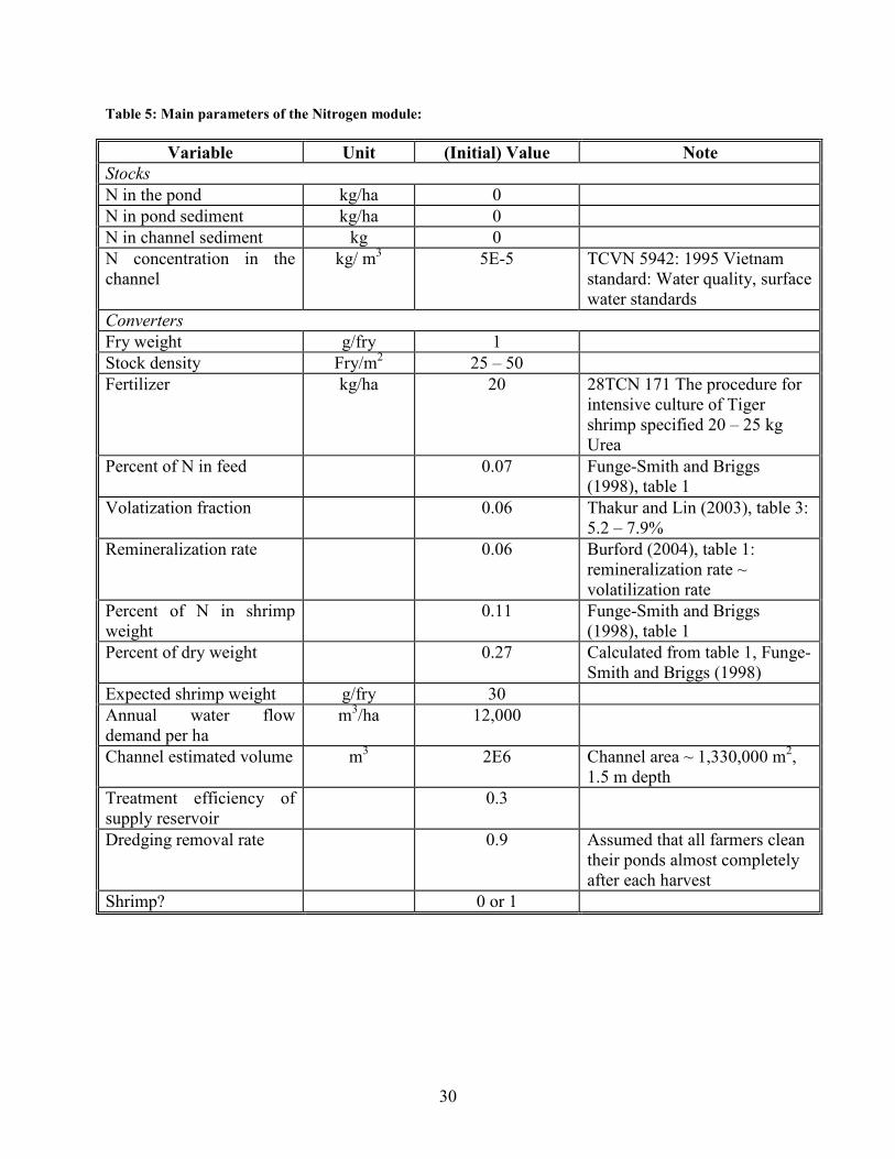
Table 5: Main parameters of the Nitrogen module:

Variable Unit (Initial) Value Note

Stocks N in the pond kg/ha 0 N in pond sediment kg/ha 0 N in channel sediment kg 0 N concentration in the channel

kg/ m3 5E-5 TCVN 5942: 1995 Vietnam standard: Water quality, surface water standards

Converters Fry weight g/fry 1 Stock density Fry/m2 25 – 50 Fertilizer kg/ha 20 28TCN 171 The procedure for

intensive culture of Tiger shrimp specified 20 – 25 kg Urea

Percent of N in feed 0.07 Funge-Smith and Briggs (1998), table 1

Volatization fraction 0.06 Thakur and Lin (2003), table 3: 5.2 – 7.9%

Remineralization rate 0.06 Burford (2004), table 1: remineralization rate ~ volatilization rate

Percent of N in shrimp weight

0.11 Funge-Smith and Briggs (1998), table 1

Percent of dry weight 0.27 Calculated from table 1, Funge-Smith and Briggs (1998)

Expected shrimp weight g/fry 30 Annual water flow demand per ha

m3/ha 12,000

Channel estimated volume m3 2E6 Channel area ~ 1,330,000 m2, 1.5 m depth

Treatment efficiency of supply reservoir

0.3

Dredging removal rate 0.9 Assumed that all farmers clean their ponds almost completely after each harvest

Shrimp? 0 or 1

31

Variable Unit Value Note

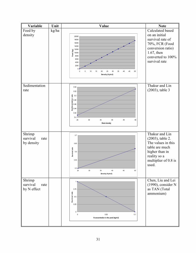
Feed by density

kg/ha

0

2000

4000

6000

8000

10000

12000

14000

16000

18000

20000

0 5 10 15 20 25 30 35 40 45 50

Density (fry/m2)

Feed (kg)

Calculated based on an initial survival rate of 70%, FCR (Food conversion ratio) 1.67, then converted to 100% survival rate

Sedimentation rate

0.4

0.42

0.44

0.46

0.48

0.5

0.52

0.54

25 30 35 40 45 50

Stock density

Sedim

entation rate

Thakur and Lin (2003), table 3

Shrimp survival rate by density

0.5

0.55

0.6

0.65

0.7

25 30 35 40 45 50

Density (fry/m2)

Survival rate

Thakur and Lin (2003), table 2. The values in this table are much higher than in reality so a multiplier of 0.8 is used.

Shrimp survival rate by N effect

0

0.25

0.5

0.75

1

0 0.05 0.1

N concentration in the pond (kg/m3)

Surv

ival ra

te

Chen, Liu and Lei (1990), consider N as TAN (Total ammonium)

32

Variable Unit Value Note

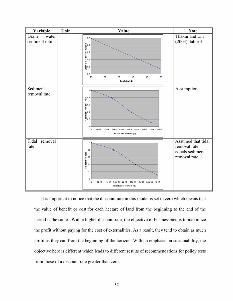
Drain water sediment ratio

0.2

0.3

0.4

0.5

0.6

0.7

25 30 35 40 45 50

Density (fry/m2)

Dra

in w

ater sedim

ent ra

tio

Thakur and Lin (2003), table 3

Sediment removal rate

0

0.2

0.4

0.6

0.8

1

0 5E+08 1E+09 1.5E+09 2E+09 2.5E+09 3E+09 3.5E+09 4E+09 4.5E+09

N in channel sediment (kg)

Sedim

ent re

moval ra

te

Assumption

Tidal removal rate

0

0.2

0.4

0.6

0.8

1

0 5E+08 1E+09 1.5E+09 2E+09 2.5E+09 3E+09 3.5E+09 4E+09

N in channel sediment (kg)

Tid

al re

moval ra

te

Assumed that tidal removal rate equals sediment removal rate

It is important to notice that the discount rate in this model is set to zero which means that

the value of benefit or cost for each hectare of land from the beginning to the end of the

period is the same. With a higher discount rate, the objective of businessmen is to maximize

the profit without paying for the cost of externalities. As a result, they tend to obtain as much

profit as they can from the beginning of the horizon. With an emphasis on sustainability, the

objective here is different which leads to different results of recommendations for policy tests

from those of a discount rate greater than zero.

33

CHAPTER FOUR

BASE CASE SIMULATIONS

In intensive shrimp farming in Vietnam, the commonly used stock density ranges from 25 –

45 fry/m2, and the higher density is more prefered by farmers. This chapter gives two base case

simulations of high and low stock densities to provide a brief comparison. The time horizon

covers 20 years from 1999 to 2019 with the assumption that pilot farms started in 2000. All the

runs are conducted with a dt of 0.25 years.

4.1 High stock density simulations

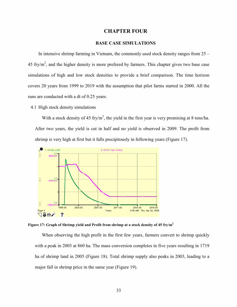
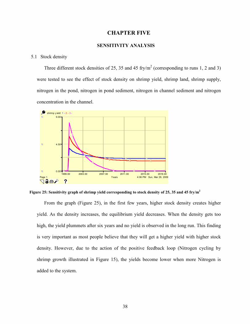
With a stock density of 45 fry/m2, the yield in the first year is very promising at 8 tons/ha.

After two years, the yield is cut in half and no yield is observed in 2009. The profit from

shrimp is very high at first but it falls precipitously in following years (Figure 17).

9:05 AM Thu, Apr 02, 2009Page 3

1999.00 2003.00 2007.00 2011.00 2015.00 2019.00

Years

1:

1:

1:

2:

2:

2:

0.0

4.5

9.0

-15000000

-5000000

5000000

1: shrimp y ield 2: Prof it f rom shrimp

1

1

11 1

2

2

2

2 2

Figure 17: Graph of Shrimp yield and Profit from shrimp at a stock density of 45 fry/m2

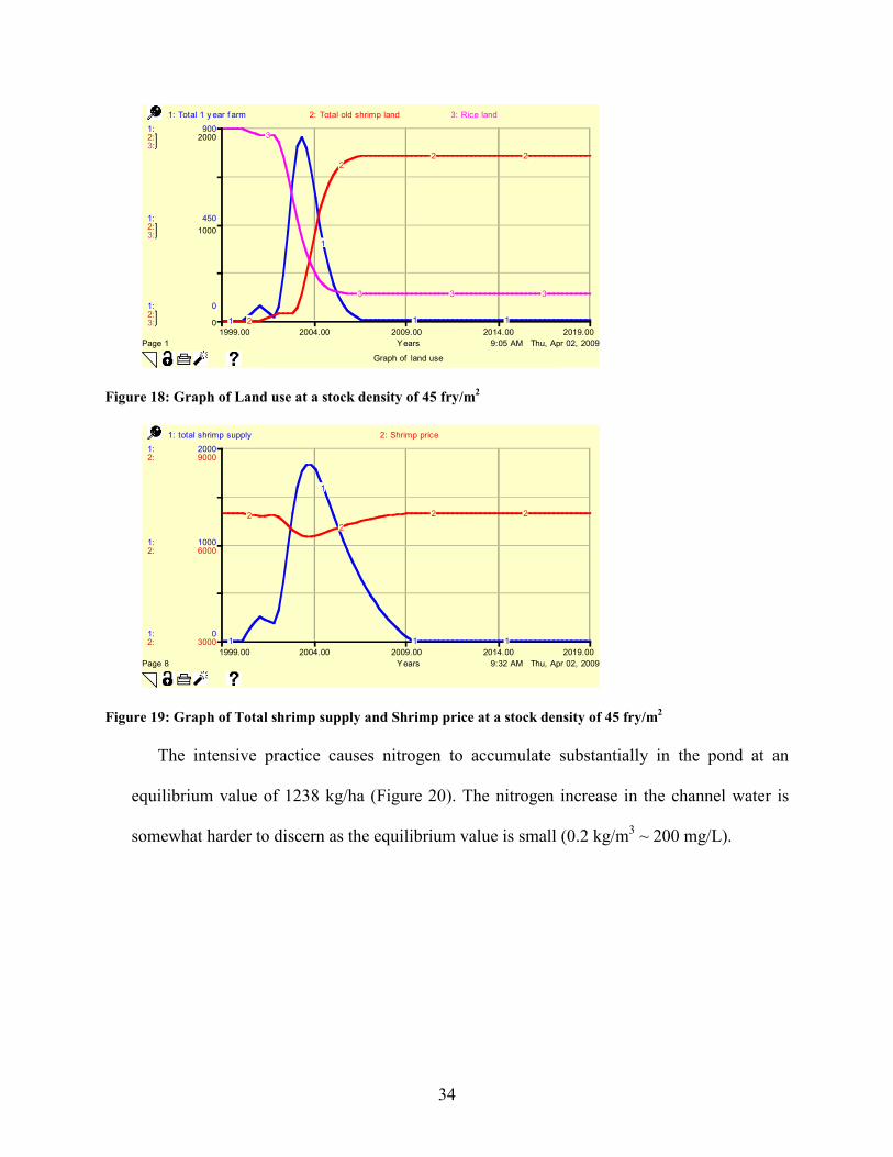
When observing the high profit in the first few years, farmers convert to shrimp quickly

with a peak in 2003 at 860 ha. The mass conversion completes in five years resulting in 1719

ha of shrimp land in 2005 (Figure 18). Total shrimp supply also peaks in 2003, leading to a

major fall in shrimp price in the same year (Figure 19).

34

9:05 AM Thu, Apr 02, 2009

Graph of land use

Page 1

1999.00 2004.00 2009.00 2014.00 2019.00

Years

1:

1:

1:

2:

2:

2:

3:

3:

3:

0

450

900

0

1000

2000

1: Total 1 y ear f arm 2: Total old shrimp land 3: Rice land

1

1

1 12

22 2

3

3 3 3

Figure 18: Graph of Land use at a stock density of 45 fry/m2

9:32 AM Thu, Apr 02, 2009Page 8

1999.00 2004.00 2009.00 2014.00 2019.00

Years

1:

1:

1:

2:

2:

2:

0

1000

2000

3000

6000

9000

1: total shrimp supply 2: Shrimp price

1

1

1 1

2

2

2 2

Figure 19: Graph of Total shrimp supply and Shrimp price at a stock density of 45 fry/m2

The intensive practice causes nitrogen to accumulate substantially in the pond at an

equilibrium value of 1238 kg/ha (Figure 20). The nitrogen increase in the channel water is

somewhat harder to discern as the equilibrium value is small (0.2 kg/m3 ~ 200 mg/L).

35

9:32 AM Thu, Apr 02, 2009Page 4

1999.00 2003.00 2007.00 2011.00 2015.00 2019.00

Years

1:

1:

1:

2:

2:

2:

3:

3:

3:

0

2500

5000

0.00

0.02

0.05

0.0

4.5

9.0

1: N in the pond 2: N concentration in the channel 3: shrimp y ield

1

1

1 1 1

2

2

22 2

3

3

3 3 3

Figure 20: Graph of Nitrogen in the pond, Nitrogen concentration in the channel and Shrimp yield at a stock

density of 45 fry/m2

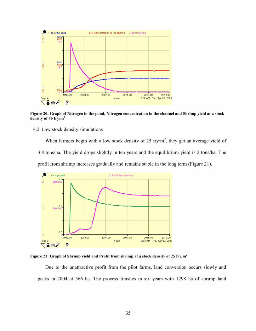
4.2 Low stock density simulations

When farmers begin with a low stock density of 25 fry/m2, they get an average yield of

3.8 tons/ha. The yield drops slightly in ten years and the equilibrium yield is 2 tons/ha. The

profit from shrimp increases gradually and remains stable in the long term (Figure 21).

9:04 AM Thu, Apr 02, 2009Page 3

1999.00 2003.00 2007.00 2011.00 2015.00 2019.00

Years

1:

1:

1:

2:

2:

2:

0.0

2.0

4.0

0

2500000

5000000


1

1

11 1

2

2

2

2 2

Figure 21: Graph of Shrimp yield and Profit from shrimp at a stock density of 25 fry/m2

Due to the unattractive profit from the pilot farms, land conversion occurs slowly and

peaks in 2004 at 566 ha. The process finishes in six years with 1298 ha of shrimp land

36

(Figure 22). Total shrimp supply also peaks in 2004, leading to a fall in shrimp price in the

same year (Figure 23).

9:04 AM Thu, Apr 02, 2009

Graph of land use

Page 1

1999.00 2004.00 2009.00 2014.00 2019.00

Years

1:

1:

1:

2:

2:

2:

3:

3:

3:

0

300

600

0

1000

2000


1

1

1 12

2

2 2

3

3 3 3

Figure 22: Graph of Land use at a stock density of 25 fry/m2

9:04 AM Thu, Apr 02, 2009Page 8

1999.00 2004.00 2009.00 2014.00 2019.00

Years

1:

1:

1:

2:

2:

2:

0

1000

2000

3000

6000

9000

1: total shrimp supply 2: Shrimp price

1

1

1 1

2

2 2 2

Figure 23: Graph of Total shrimp supply and Shrimp price at a stock density of 25 fry/m2

With a low stock density, the shrimp farming practice is not highly intensive. The

nitrogen content in the pond is around 550 kg/ha and nitrogen concentration in the channel is

also low, roughly 0.01 kg/m3 (100 mg/L). Due to the low accumulation of nitrogen in the

system, the yield is sustainable till the end of the horizon*.

* Although this practice is good for the environment, this may not be the preferable practice in the case of a positive discount rate.

37

9:04 AM Thu, Apr 02, 2009Page 4

1999.00 2003.00 2007.00 2011.00 2015.00 2019.00

Years

1:

1:

1:

2:

2:

2:

3:

3:

3:

0

2500

5000

0.00

0.02

0.05

0.0

2.0

4.0


1

11 1 1

2

2

2 2 2

3

3

3 3 3

Figure 24: Graph of Nitrogen in the pond, Nitrogen concentration in the channel and Shrimp yield at a stock

density of 25 fry/m2

From the two base case simulations, it is obvious that higher stock density gives a higher

yield at first and speeds up the conversion process. However, the unsustainable practice

endangers the system by introducing too much nutrient content and puts farmers into trouble

with no yield in the long run.

38

CHAPTER FIVE

SENSITIVITY ANALYSIS

5.1 Stock density

Three different stock densities of 25, 35 and 45 fry/m2 (corresponding to runs 1, 2 and 3)

were tested to see the effect of stock density on shrimp yield, shrimp land, shrimp supply,

nitrogen in the pond, nitrogen in pond sediment, nitrogen in channel sediment and nitrogen

concentration in the channel.

4:06 PM Sun, Mar 29, 2009Page 1

1999.00 2003.00 2007.00 2011.00 2015.00 2019.00

Years

1:

1:

1:

0.00

4.50

9.00

shrimp y ield: 1 - 2 - 3 -

1

11 1 1

22

2 2 2

3

3

3 3 3

Figure 25: Sensitivity graph of shrimp yield corresponding to stock density of 25, 35 and 45 fry/m2

From the graph (Figure 25), in the first few years, higher stock density creates higher

yield. As the density increases, the equilibrium yield decreases. When the density gets too

high, the yield plummets after six years and no yield is observed in the long run. This finding

is very important as most people believe that they will get a higher yield with higher stock

density. However, due to the action of the positive feedback loop (Nitrogen cycling by

shrimp growth illustrated in Figure 15), the yields become lower when more Nitrogen is

added to the system.

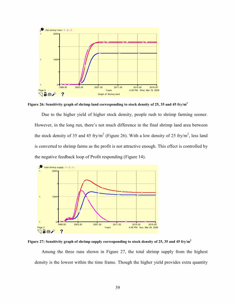
39

4:09 PM Wed, Mar 18, 2009

Graph of Shrimp land

Page 5

1999.00 2003.00 2007.00 2011.00 2015.00 2019.00

Years

1:

1:

1:

0

1000

2000

Old shrimp f arm: 1 - 2 - 3 -

1 1

1 1 1

2

2

2 2 2

3

3

3 3 3

Figure 26: Sensitivity graph of shrimp land corresponding to stock density of 25, 35 and 45 fry/m2

Due to the higher yield of higher stock density, people rush to shrimp farming sooner.

However, in the long run, there’s not much difference in the final shrimp land area between

the stock density of 35 and 45 fry/m2 (Figure 26). With a low density of 25 fry/m2, less land

is converted to shrimp farms as the profit is not attractive enough. This effect is controlled by

the negative feedback loop of Profit responding (Figure 14).

4:06 PM Sun, Mar 29, 2009Page 2

1999.00 2003.00 2007.00 2011.00 2015.00 2019.00

Years

1:

1:

1:

0

1500

3000

total shrimp supply : 1 - 2 - 3 -

1

1

11 1

2

2

2

2 2

3

3

3 3 3

Figure 27: Sensitivity graph of shrimp supply corresponding to stock density of 25, 35 and 45 fry/m2

Among the three runs shown in Figure 27, the total shrimp supply from the highest

density is the lowest within the time frame. Though the higher yield provides extra quantity

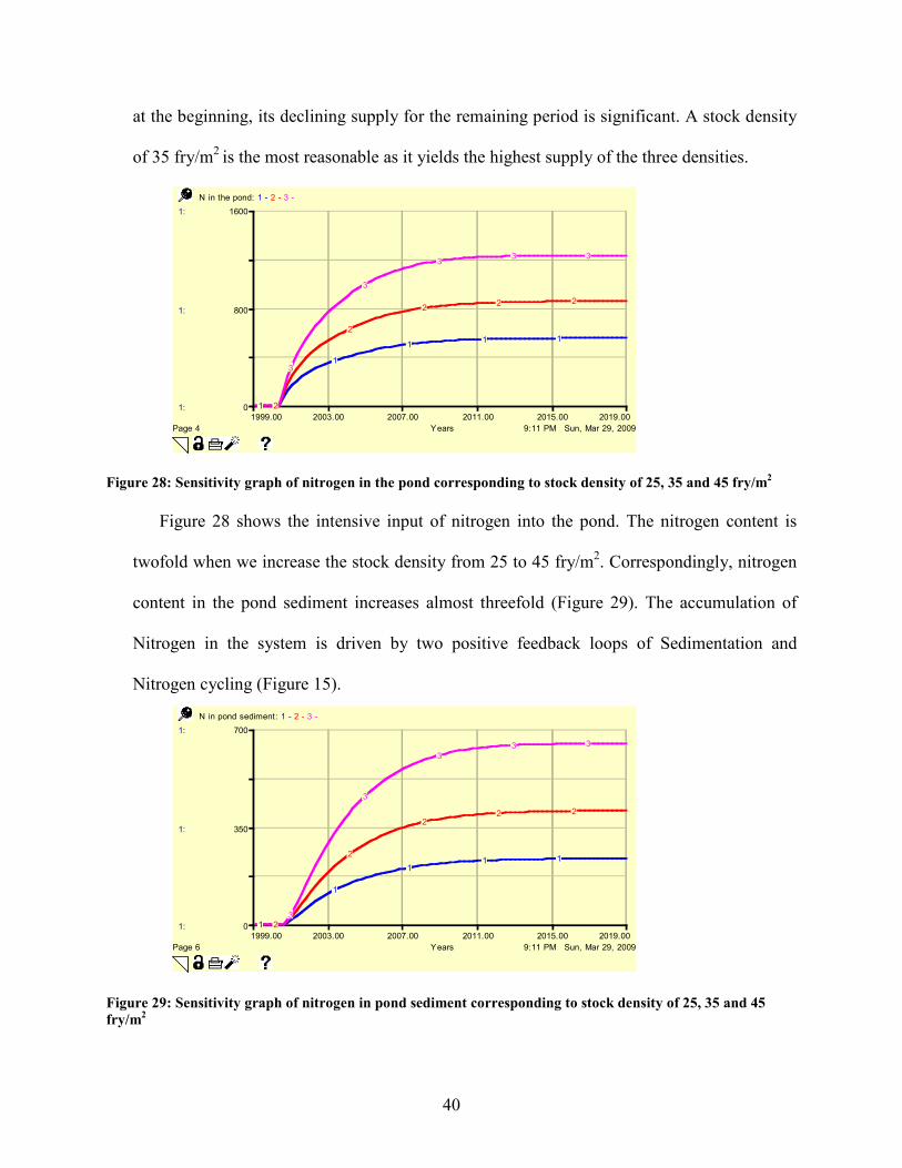
40

at the beginning, its declining supply for the remaining period is significant. A stock density

of 35 fry/m2 is the most reasonable as it yields the highest supply of the three densities.

9:11 PM Sun, Mar 29, 2009Page 4

1999.00 2003.00 2007.00 2011.00 2015.00 2019.00

Years

1:

1:

1:

0

800

1600

N in the pond: 1 - 2 - 3 -

1

1

11 1

2

2

22 2

3

3

33 3

Figure 28: Sensitivity graph of nitrogen in the pond corresponding to stock density of 25, 35 and 45 fry/m2

Figure 28 shows the intensive input of nitrogen into the pond. The nitrogen content is

twofold when we increase the stock density from 25 to 45 fry/m2. Correspondingly, nitrogen

content in the pond sediment increases almost threefold (Figure 29). The accumulation of

Nitrogen in the system is driven by two positive feedback loops of Sedimentation and

Nitrogen cycling (Figure 15).

9:11 PM Sun, Mar 29, 2009Page 6

1999.00 2003.00 2007.00 2011.00 2015.00 2019.00

Years

1:

1:

1:

0

350

700

N in pond sediment: 1 - 2 - 3 -

1

1

11 1

2

2

22 2

3

3

33 3

Figure 29: Sensitivity graph of nitrogen in pond sediment corresponding to stock density of 25, 35 and 45

fry/m2

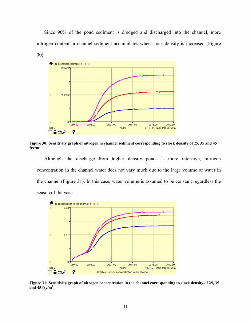
41

Since 90% of the pond sediment is dredged and discharged into the channel, more

nitrogen content in channel sediment accumulates when stock density is increased (Figure

30).

9:11 PM Sun, Mar 29, 2009Page 7

1999.00 2003.00 2007.00 2011.00 2015.00 2019.00

Years

1:

1:

1:

0

350000

700000

N in channel sediment: 1 - 2 - 3 -

1 1

11 1

2

2

2

2 2

3

3

3

3 3

Figure 30: Sensitivity graph of nitrogen in channel sediment corresponding to stock density of 25, 35 and 45

fry/m2

Although the discharge from higher density ponds is more intensive, nitrogen

concentration in the channel water does not vary much due to the large volume of water in

the channel (Figure 31). In this case, water volume is assumed to be constant regardless the

season of the year.

4:09 PM Wed, Mar 18, 2009

Graph of Nitrogen concentration in the channel

Page 3

1999.00 2003.00 2007.00 2011.00 2015.00 2019.00

Years

1:

1:

1:

0

0.01

0.02

N concentration in the channel: 1 - 2 - 3 -

1

1

1

1 1

2

2

2

2 2

3

3

33 3

Figure 31: Sensitivity graph of nitrogen concentration in the channel corresponding to stock density of 25, 35

and 45 fry/m2

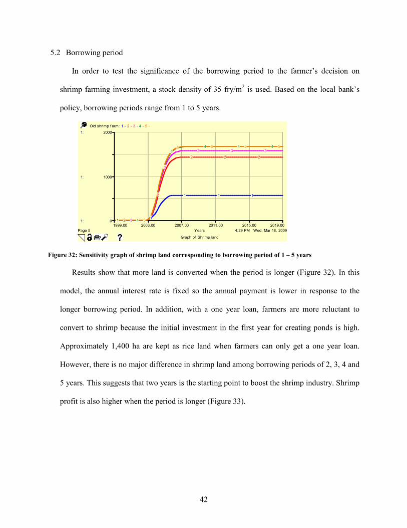
42

5.2 Borrowing period

In order to test the significance of the borrowing period to the farmer’s decision on

shrimp farming investment, a stock density of 35 fry/m2 is used. Based on the local bank’s

policy, borrowing periods range from 1 to 5 years.

4:29 PM Wed, Mar 18, 2009

Graph of Shrimp land

Page 5

1999.00 2003.00 2007.00 2011.00 2015.00 2019.00

Years

1:

1:

1:

0

1000

2000

Old shrimp f arm: 1 - 2 - 3 - 4 - 5 -

11

1 1 1

2

2

2 2 2

3

3

3 3 3

4

4

4 4 4

5

5 5 5 5

Figure 32: Sensitivity graph of shrimp land corresponding to borrowing period of 1 – 5 years

Results show that more land is converted when the period is longer (Figure 32). In this

model, the annual interest rate is fixed so the annual payment is lower in response to the

longer borrowing period. In addition, with a one year loan, farmers are more reluctant to

convert to shrimp because the initial investment in the first year for creating ponds is high.

Approximately 1,400 ha are kept as rice land when farmers can only get a one year loan.

However, there is no major difference in shrimp land among borrowing periods of 2, 3, 4 and

5 years. This suggests that two years is the starting point to boost the shrimp industry. Shrimp

profit is also higher when the period is longer (Figure 33).

43

9:18 AM Thu, Apr 02, 2009Page 8

1999.00 2004.00 2009.00 2014.00 2019.00

Years

1:

1:

1:

-2500000

500000

3500000

Prof it f rom shrimp: 1 - 2 - 3 - 4 - 5 -

1

1

11

2

2

2

2

3

3

3

3

4

4

44

5

5

55

Figure 33: Sensitivity graph of shrimp profit corresponding to borrowing period of 1 – 5 years

5.3 Tidal removal rate

Tidal removal rate is considered for testing because it helps decrease the nitrogen content

in channel water and consequently reduces the nitrogen content in intake water. However,

there is little knowledge on the tidal removal rate in this region. It is also not easy to judge

whether the tidal removal rate depends on sediment load in the channel and hence it also

depends on sediment removal rate. Two main scenarios are built for this test: (1) tidal

removal rate depends on sediment load in the channel and (2) tidal removal rate is

independent of sediment load in the channel. For the first scenario, three cases are

considered: (1) tidal removal and sediment removal rates are equal, (2) tidal removal rate is

linearly dependent on sediment load and (3) tidal removal rate is hyperbolic dependent on

sediment load. A stock density of 35 fry/m2 and a borrowing period of 5 years are used in

this test.

For the first scenario, there is no difference in shrimp yield among the three cases (Figure

34). This shows that the interdependence between tidal removal rate and sediment load is

negligible.

44

5:05 PM Wed, Mar 18, 2009

Graph of shrimp y ield

Page 1

1999.00 2003.00 2007.00 2011.00 2015.00 2019.00

Years

1:

1:

1:

0.00

3.00

6.00


1

1

11 1

2

2

22 2

3

3

33 3

Figure 34: Sensitivity graph of shrimp yield corresponding to different tidal removal rate scenario 1

For the second scenario, sensitivity runs are conducted for three tidal removal rates of

0.1, 0.5 and 0.9 corresponding to runs 1, 2 and 3. With a very low removal rate of 0.1,

farmers get no yield in six years because the high nitrogen content builds up in the system. At

a rate of 0.5, no yield will be observed in 2009. At a high removal rate of 0.9, the yield drops

from 6.9 tons/ha to 1.5 tons/ha in seven years and 0.7 tons/ha is the equilibrium yield (Figure

35).

4:32 PM Sun, Mar 29, 2009Page 1

1999.00 2003.00 2007.00 2011.00 2015.00 2019.00

Years

1:

1:

1:

0.00

3.50

7.00


1

1

1 1 1

2

2

22 2

3

3

33 3

Figure 35: Sensitivity graph of shrimp yield corresponding to tidal removal rate of 0.1, 0.5 and 0.9

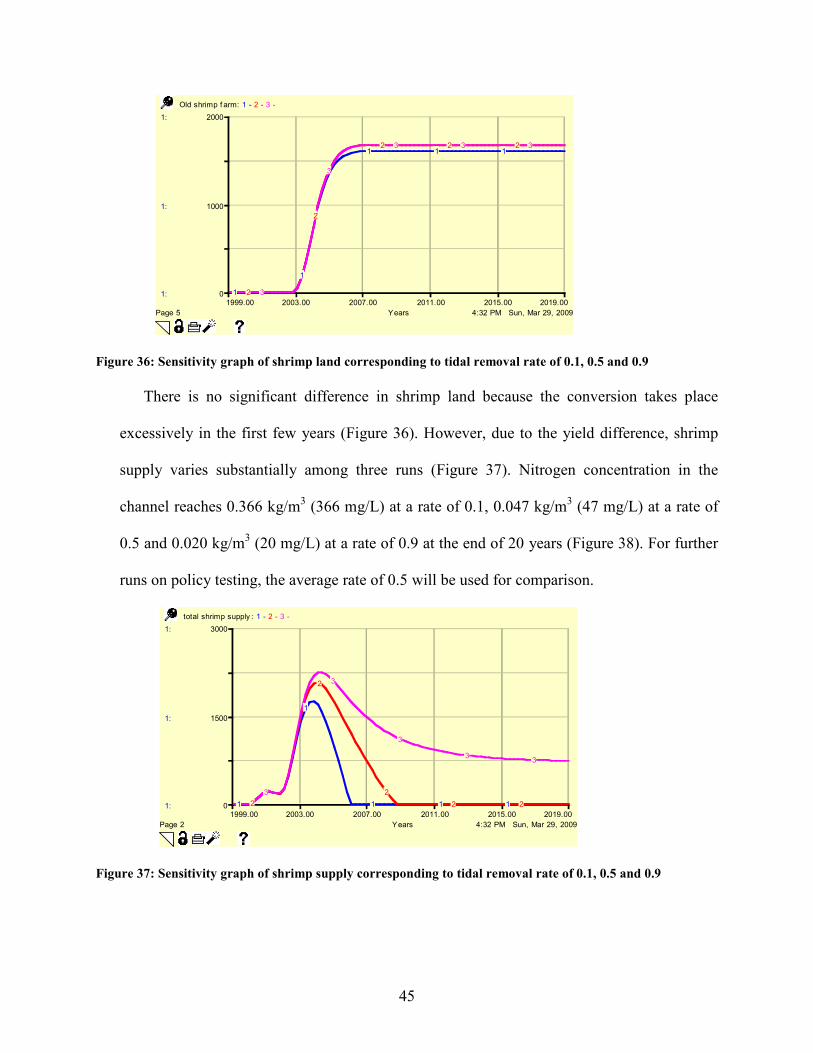
45

4:32 PM Sun, Mar 29, 2009Page 5

1999.00 2003.00 2007.00 2011.00 2015.00 2019.00

Years

1:

1:

1:

0

1000

2000

Old shrimp f arm: 1 - 2 - 3 -

1

1

1 1 1

2

2

2 2 2

3

3

3 3 3

Figure 36: Sensitivity graph of shrimp land corresponding to tidal removal rate of 0.1, 0.5 and 0.9

There is no significant difference in shrimp land because the conversion takes place

excessively in the first few years (Figure 36). However, due to the yield difference, shrimp

supply varies substantially among three runs (Figure 37). Nitrogen concentration in the

channel reaches 0.366 kg/m3 (366 mg/L) at a rate of 0.1, 0.047 kg/m3 (47 mg/L) at a rate of

0.5 and 0.020 kg/m3 (20 mg/L) at a rate of 0.9 at the end of 20 years (Figure 38). For further

runs on policy testing, the average rate of 0.5 will be used for comparison.

4:32 PM Sun, Mar 29, 2009Page 2

1999.00 2003.00 2007.00 2011.00 2015.00 2019.00

Years

1:

1:

1:

0

1500

3000


1

1

1 1 12

2

2

2 2

3

3

3

33

Figure 37: Sensitivity graph of shrimp supply corresponding to tidal removal rate of 0.1, 0.5 and 0.9

46

4:32 PM Sun, Mar 29, 2009Page 3

1999.00 2003.00 2007.00 2011.00 2015.00 2019.00

Years

1:

1:

1:

0

0.2

0.4

N concentration in the channel: 1 - 2 - 3 -

11

1

1

1

22

2 2 2

33 3 3 3

Figure 38: Sensitivity graph of nitrogen concentration in the channel corresponding to tidal removal rate of

0.1, 0.5 and 0.9

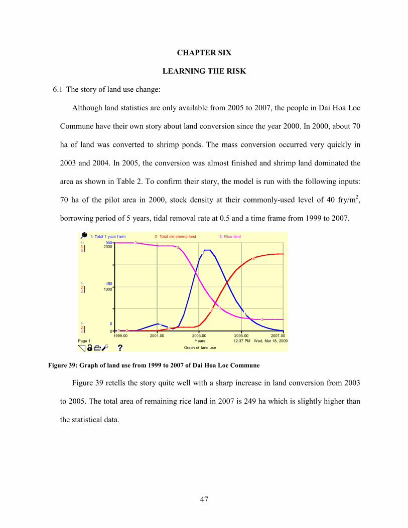
47

CHAPTER SIX

LEARNING THE RISK

6.1 The story of land use change:

Although land statistics are only available from 2005 to 2007, the people in Dai Hoa Loc

Commune have their own story about land conversion since the year 2000. In 2000, about 70

ha of land was converted to shrimp ponds. The mass conversion occurred very quickly in

2003 and 2004. In 2005, the conversion was almost finished and shrimp land dominated the

area as shown in Table 2. To confirm their story, the model is run with the following inputs:

70 ha of the pilot area in 2000, stock density at their commonly-used level of 40 fry/m2,

borrowing period of 5 years, tidal removal rate at 0.5 and a time frame from 1999 to 2007.

12:37 PM Wed, Mar 18, 2009

Graph of land use

Page 1

1999.00 2001.00 2003.00 2005.00 2007.00

Years

1:

1:

1:

2:

2:

2:

3:

3:

3:

0

450

900

0

1000

2000


1

1

1

1

2 2

2

2

33

3

3

Figure 39: Graph of land use from 1999 to 2007 of Dai Hoa Loc Commune

Figure 39 retells the story quite well with a sharp increase in land conversion from 2003

to 2005. The total area of remaining rice land in 2007 is 249 ha which is slightly higher than

the statistical data.

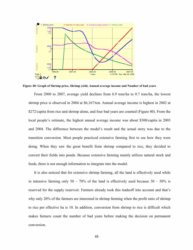
48

4:18 PM Sun, Mar 29, 2009Page 7

1999.00 2001.00 2003.00 2005.00 2007.00

Years

1:

1:

1:

2:

2:

2:

3:

3:

3:

4:

4:

4:

6000

6500

7000

0

2

4

-1000

0

1000

0.0

4.0

8.0

1: Shrimp price 2: Number of bad y ears 3: annual av erage income 4: shrimp y ield

1

1

11

2 2

2

2

33

3

3

4

4

4

4

Figure 40: Graph of Shrimp price, Shrimp yield, Annual average income and Number of bad years

From 2000 to 2007, average yield declines from 6.9 tons/ha to 0.7 tons/ha, the lowest

shrimp price is observed in 2004 at $6,167/ton. Annual average income is highest in 2002 at

$272/capita from rice and shrimp alone, and four bad years are counted (Figure 40). From the

local people’s estimate, the highest annual average income was about $300/capita in 2003

and 2004. The difference between the model’s result and the actual story was due to the

transition conversion. Most people practiced extensive farming first to see how they were

doing. When they saw the great benefit from shrimp compared to rice, they decided to

convert their fields into ponds. Because extensive farming mainly utilizes natural stock and

feeds, there is not enough information to integrate into the model.

It is also noticed that for extensive shrimp farming, all the land is effectively used while

in intensive farming only 50 – 70% of the land is effectively used because 30 – 50% is

reserved for the supply reservoir. Farmers already took this tradeoff into account and that’s

why only 20% of the farmers are interested in shrimp farming when the profit ratio of shrimp

to rice per effective ha is 10. In addition, conversion from shrimp to rice is difficult which

makes farmers count the number of bad years before making the decision on permanent

conversion.

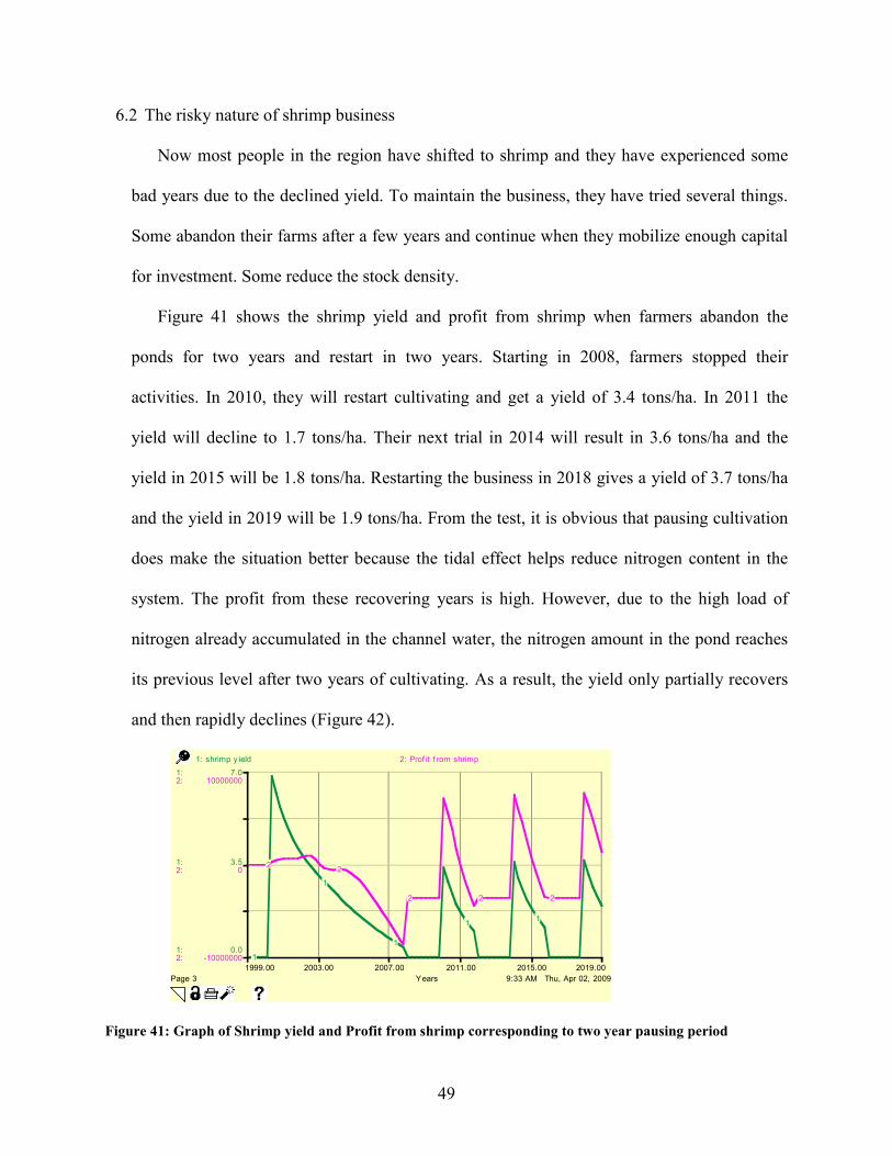
49

6.2 The risky nature of shrimp business

Now most people in the region have shifted to shrimp and they have experienced some

bad years due to the declined yield. To maintain the business, they have tried several things.

Some abandon their farms after a few years and continue when they mobilize enough capital

for investment. Some reduce the stock density.

Figure 41 shows the shrimp yield and profit from shrimp when farmers abandon the

ponds for two years and restart in two years. Starting in 2008, farmers stopped their

activities. In 2010, they will restart cultivating and get a yield of 3.4 tons/ha. In 2011 the

yield will decline to 1.7 tons/ha. Their next trial in 2014 will result in 3.6 tons/ha and the

yield in 2015 will be 1.8 tons/ha. Restarting the business in 2018 gives a yield of 3.7 tons/ha

and the yield in 2019 will be 1.9 tons/ha. From the test, it is obvious that pausing cultivation

does make the situation better because the tidal effect helps reduce nitrogen content in the

system. The profit from these recovering years is high. However, due to the high load of

nitrogen already accumulated in the channel water, the nitrogen amount in the pond reaches

its previous level after two years of cultivating. As a result, the yield only partially recovers

and then rapidly declines (Figure 42).

9:33 AM Thu, Apr 02, 2009Page 3

1999.00 2003.00 2007.00 2011.00 2015.00 2019.00

Years

1:

1:

1:

2:

2:

2:

0.0

3.5

7.0

-10000000

0

10000000


1

1

1

11

22

2 2 2

Figure 41: Graph of Shrimp yield and Profit from shrimp corresponding to two year pausing period

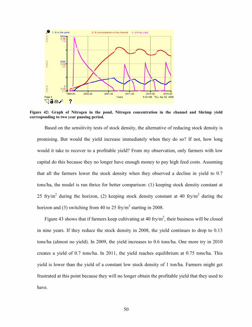
50

9:33 AM Thu, Apr 02, 2009Page 4

1999.00 2003.00 2007.00 2011.00 2015.00 2019.00

Years

1:

1:

1:

2:

2:

2:

3:

3:

3:

0

2500

5000

0.00

0.02

0.05

0.0

3.5

7.0


1

1

11 1

2

2

2 2 2

3

3

3 3 3

Figure 42: Graph of Nitrogen in the pond, Nitrogen concentration in the channel and Shrimp yield

corresponding to two year pausing period.

Based on the sensitivity tests of stock density, the alternative of reducing stock density is

promising. But would the yield increase immediately when they do so? If not, how long

would it take to recover to a profitable yield? From my observation, only farmers with low

capital do this because they no longer have enough money to pay high feed costs. Assuming

that all the farmers lower the stock density when they observed a decline in yield to 0.7

tons/ha, the model is run thrice for better comparison: (1) keeping stock density constant at

25 fry/m2 during the horizon, (2) keeping stock density constant at 40 fry/m2 during the

horizon and (3) switching from 40 to 25 fry/m2 starting in 2008.

Figure 43 shows that if farmers keep cultivating at 40 fry/m2, their business will be closed

in nine years. If they reduce the stock density in 2008, the yield continues to drop to 0.13

tons/ha (almost no yield). In 2009, the yield increases to 0.6 tons/ha. One more try in 2010

creates a yield of 0.7 tons/ha. In 2011, the yield reaches equilibrium at 0.75 tons/ha. This

yield is lower than the yield of a constant low stock density of 1 ton/ha. Farmers might get

frustrated at this point because they will no longer obtain the profitable yield that they used to

have.

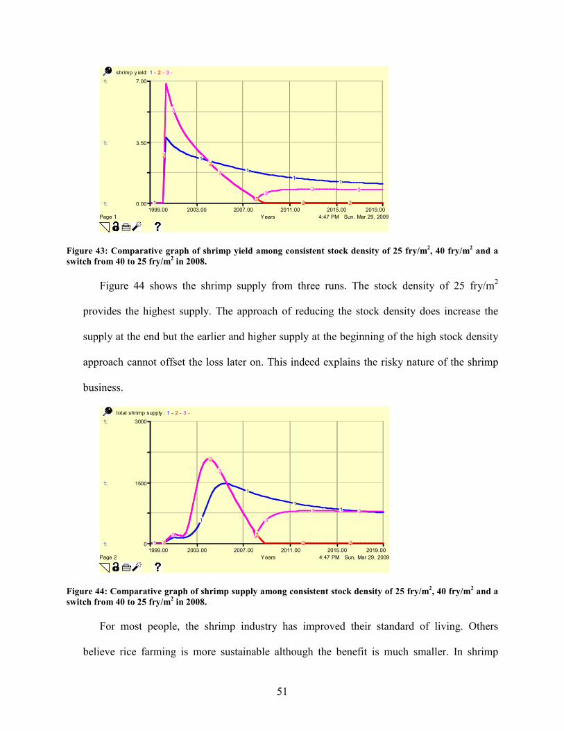
51

4:47 PM Sun, Mar 29, 2009Page 1

1999.00 2003.00 2007.00 2011.00 2015.00 2019.00

Years

1:

1:

1:

0.00

3.50

7.00


1

1

1

11

2

2

22 2

3

3

33 3

Figure 43: Comparative graph of shrimp yield among consistent stock density of 25 fry/m2, 40 fry/m

2 and a

switch from 40 to 25 fry/m2 in 2008.

Figure 44 shows the shrimp supply from three runs. The stock density of 25 fry/m2

provides the highest supply. The approach of reducing the stock density does increase the

supply at the end but the earlier and higher supply at the beginning of the high stock density

approach cannot offset the loss later on. This indeed explains the risky nature of the shrimp

business.

4:47 PM Sun, Mar 29, 2009Page 2

1999.00 2003.00 2007.00 2011.00 2015.00 2019.00

Years

1:

1:

1:

0

1500

3000


1

1

1

11

2

2

2

2 2

3

3

3

3 3

Figure 44: Comparative graph of shrimp supply among consistent stock density of 25 fry/m2, 40 fry/m

2 and a

switch from 40 to 25 fry/m2 in 2008.

For most people, the shrimp industry has improved their standard of living. Others

believe rice farming is more sustainable although the benefit is much smaller. In shrimp

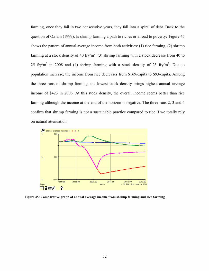
52

farming, once they fail in two consecutive years, they fall into a spiral of debt. Back to the

question of Oxfam (1999): Is shrimp farming a path to riches or a road to poverty? Figure 45

shows the pattern of annual average income from both activities: (1) rice farming, (2) shrimp

farming at a stock density of 40 fry/m2, (3) shrimp farming with a stock decrease from 40 to

25 fry/m2 in 2008 and (4) shrimp farming with a stock density of 25 fry/m2. Due to

population increase, the income from rice decreases from $169/capita to $93/capita. Among

the three runs of shrimp farming, the lowest stock density brings highest annual average

income of $423 in 2006. At this stock density, the overall income seems better than rice

farming although the income at the end of the horizon is negative. The three runs 2, 3 and 4

confirm that shrimp farming is not a sustainable practice compared to rice if we totally rely

on natural attenuation.

5:00 PM Sun, Mar 29, 2009Page 11

1999.00 2003.00 2007.00 2011.00 2015.00 2019.00

Years

1:

1:

1:

-1500

-500

500

annual av erage income: 1 - 2 - 3 - 4 -

1 1 1 1 12

2

2 2

2

3

3

3

3 3

4

4

4

44

Figure 45: Comparative graph of annual average income from shrimp farming and rice farming

53

CHAPTER SEVEN

POLICY TESTING

Scientists believe that farmers have to assign treatment ponds to treat the drainage from

harvest before discharging into the environment and that the channel system should be improved

to facilitate this industry. In this section, these two recommendations are considered for testing.

7.1 Improving the channel system

The purpose of improving the channel system is to enhance the tidal removal rate and

subsequently reduce the nitrogen concentration in the channel. Due to the crisscrossing

channel system in this area, the hydraulic condition is very complicated. Investment in

infrastructure development is costly so the model will be used to test if this investment is

worthwhile.

Suppose that the tidal removal rate increases from 0.5 to 0.75. Four runs are conducted

for comparison: (1) stock density is kept constant at 40 during the horizon and tidal removal

rate is set to 0.75 in 2008, (2) in 2008 stock density is reduced from 40 to 25 and tidal

removal rate increased from 0.5 to 0.75 (3) stock density is kept constant at 25 and tidal

removal rate is 0.5 and (4) stock density is reduced from 40 to 25 in 2008 keeping the tidal

removal rate at 0.5.

Results show that improving the channel without reducing the stock density creates the

lowest yield of 0.15 tons/ha at the end of the 20-year run. Lowering the stock without

improving the channel system helps sustain the yield at 0.75 tons/ha. The best strategy is to

improve the channel and lower the stock density at the same time to maintain the yield at 1.6

tons/ha (Figure 46). Correspondingly, the supply of the second run is highest (Figure 47).

54

5:08 PM Sun, Mar 29, 2009Page 1

1999.00 2003.00 2007.00 2011.00 2015.00 2019.00

Years

1:

1:

1:

0.00

3.50

7.00

shrimp y ield: 1 - 2 - 3 - 4 -

1

1

1

1 1

2

2

2

22

3

3

33

3

4

4

4 4 4

Figure 46: Graph of Shrimp yield in the test of improving the channel system

5:08 PM Sun, Mar 29, 2009Page 2

1999.00 2003.00 2007.00 2011.00 2015.00 2019.00

Years

1:

1:

1:

0

1500

3000

total shrimp supply : 1 - 2 - 3 - 4 -

1

1

1

11

2

2

2

2

2

3

3

3

33

4

4

44 4

Figure 47: Graph of Shrimp supply in the test of improving the channel system

From the profit perspective, only profit from improving the channel and lowering stock is

considerable. The profit of this strategy at the end of the period is around 2 million dollars.

From Figure 46, the yield of this approach is sustainable so the profit is also sustained in

Figure 48. The profit in the long term is so large that it is worthwhile to invest in

infrastructure development. In reality, such a large project can only be managed by the

government and the process may take a long time. Another approach is that each farmer has

his own treatment pond to treat the drainage water before discharging into the channel.

55

5:08 PM Sun, Mar 29, 2009Page 8

1999.00 2004.00 2009.00 2014.00 2019.00

Years

1:

1:

1:

-15000000

-5000000

5000000

Prof it f rom shrimp: 1 - 2 - 3 - 4 -

11

11

2

2 2

2

3

3

33

4

4

4 4

Figure 48: Graph of shrimp profit in the test of improving the channel system

7.2 Assigning treatment pond

By standard 28TCN 171 (2001), each farm should reserve 20 – 25% of the land for a

supply reservoir, 10 – 15% for a treatment pond and the rest is used for growing shrimp. In

practice, farmers reserve 30 – 50% of their land for a supply reservoir instead of dividing the

land into two different ponds. Suppose that we change from the current practice to strictly

comply with the standard, the treatment efficiency of the supply reservoir is reduced by half,

i.e., from 30% to 15%. According to Teichert-Coddington, Rouse, Potts and Boyd (1999), the

treatment pond helps reduce 7% of total nitrogen in the pond or its treatment efficiency is

31%. In this analysis, two base runs of stock density of 25 and 40 without any change are

maintained for comparison. Two new runs are added: (3) keep the stock density constant at

40 and introduce the treatment pond in 2008 and (4) while introducing a treatment pond in

2008, reduce the stock density from 40 to 25.

Results show that with a stock density of 40, the introduction of treatment ponds does not

help improve the situation. Combining treatment ponds with lowering the stock density

recovers the yield to 1 ton/ha – the level of applying a constant low stock density at the

beginning (Figure 49). Yield recovery increases shrimp supply (Figure 50) and shrimp profit

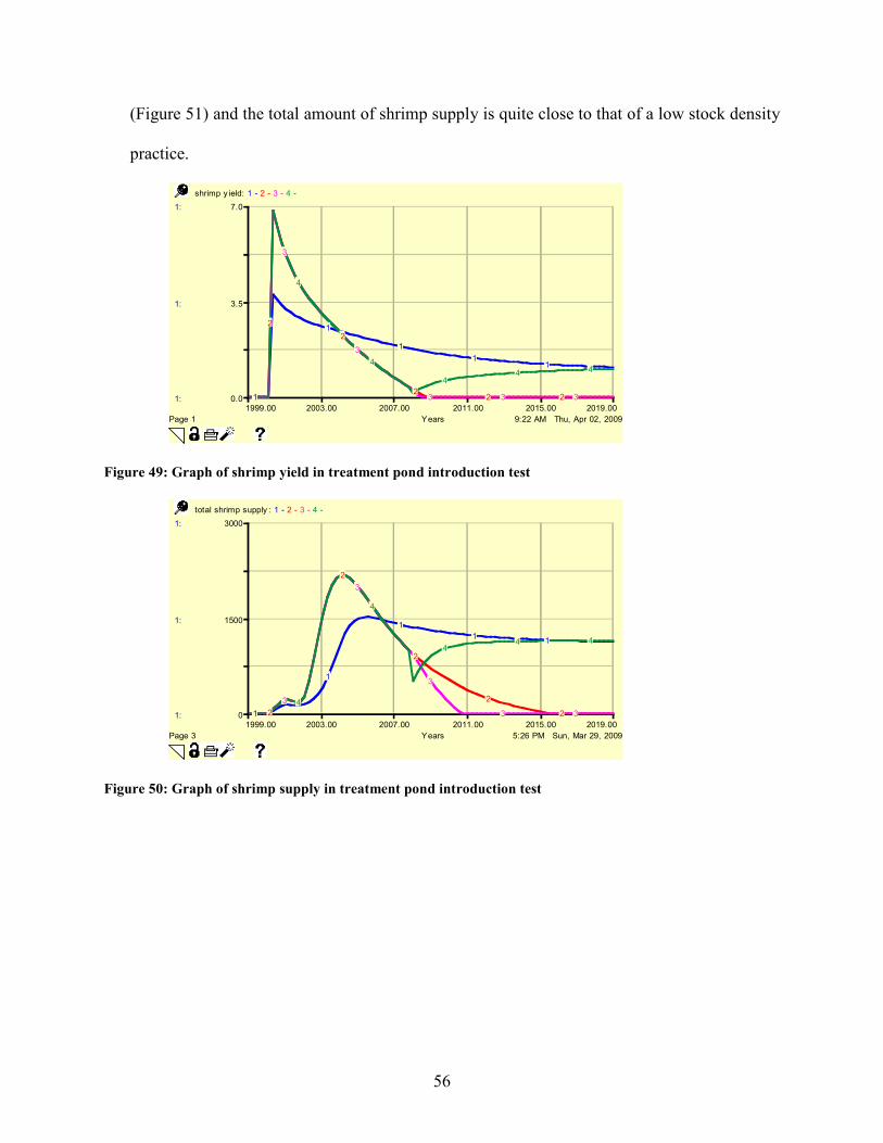
56

(Figure 51) and the total amount of shrimp supply is quite close to that of a low stock density

practice.

9:22 AM Thu, Apr 02, 2009Page 1

1999.00 2003.00 2007.00 2011.00 2015.00 2019.00

Years

1:

1:

1:

0.0

3.5

7.0

shrimp y ield: 1 - 2 - 3 - 4 -

1

1

1

11

2

2

22 2

3

3

3 3 3

4

4

44 4

Figure 49: Graph of shrimp yield in treatment pond introduction test

5:26 PM Sun, Mar 29, 2009Page 3

1999.00 2003.00 2007.00 2011.00 2015.00 2019.00

Years

1:

1:

1:

0

1500

3000

total shrimp supply : 1 - 2 - 3 - 4 -

1

1

1

11

2

2

2

2

2

3

3

3

3 3

4

4

44 4

Figure 50: Graph of shrimp supply in treatment pond introduction test

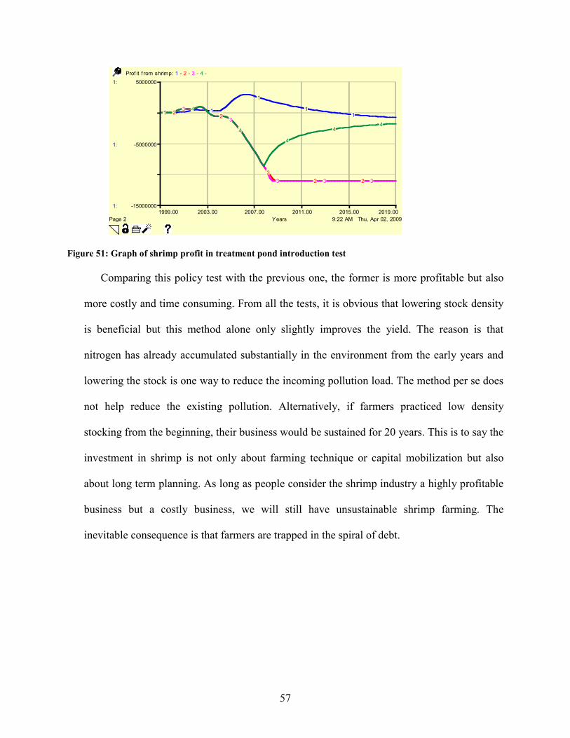
57

9:22 AM Thu, Apr 02, 2009Page 2

1999.00 2003.00 2007.00 2011.00 2015.00 2019.00

Years

1:

1:

1:

-15000000

-5000000

5000000

Prof it f rom shrimp: 1 - 2 - 3 - 4 -

1 1

1

112

2

2

2 2

3

3

3 3 3

4

4

4

44

Figure 51: Graph of shrimp profit in treatment pond introduction test

Comparing this policy test with the previous one, the former is more profitable but also

more costly and time consuming. From all the tests, it is obvious that lowering stock density

is beneficial but this method alone only slightly improves the yield. The reason is that

nitrogen has already accumulated substantially in the environment from the early years and

lowering the stock is one way to reduce the incoming pollution load. The method per se does

not help reduce the existing pollution. Alternatively, if farmers practiced low density

stocking from the beginning, their business would be sustained for 20 years. This is to say the

investment in shrimp is not only about farming technique or capital mobilization but also

about long term planning. As long as people consider the shrimp industry a highly profitable

business but a costly business, we will still have unsustainable shrimp farming. The

inevitable consequence is that farmers are trapped in the spiral of debt.

58

CHAPTER EIGHT

FURTHER WORK AND CONCLUSION

8.1 Further work

There are opportunities to discuss some interesting issues in the future version of the

model such as the relationship between monopsony market and externalities, and the

application of taxing in regulating farmers’ practice. With the monopsony power, buyers

purchase a smaller quantity compared to that of a competitive market. This quantity shifts

toward the quantity of a market where externalities are partially accounted for shrimp price.

This is to say monopsony structure in the presence of externalities can reduce the deadweight

loss. In addition, based on the results of this model, the government might want to impose a

low stock density use. This could be done in several ways and taxing on fry is a promising

approach. Theoretically, this tax should be equal to the marginal value of externalities so that

externalities are internalized in shrimp farming. In reality, the success of such policy depends

on many factors and the answer can only be found in future research.

8.2 Summary and conclusion

The model built for the case of Dai Hoa Loc Commune has shed light on the economic

incentive for local farmers to shift from rice to shrimp farming which has led to dynamic land

use change in the last 10 years. In addition, modeling the interaction of shrimp farming and

the environment also reveals the risky nature of the shrimp industry. Although farmers are

very careful in taking training courses and observing the number of bad years before deciding

to change, high profit is only obtained in the first few years. When there is a major decline in

shrimp yield due to the cumulative impact of nutrient pollution in the system, most people

fall into the spiral of debt. The serious problem here is that the higher stock density used at

59

the beginning, the shorter time the system lasts. Another issue is that converting back from

shrimp to rice is difficult and considered to be impractical. Once the move to shrimp is made,

they are trapped in this business forever.

In order to improve the system, two policies were tested. Results show that a combination

of lowering the stock density from 40 to 25 fry/m2 and introducing treatment ponds helps

sustain the business within the horizon. A better approach is to improve the channel system

in addition to lowering the stock density. This strategy shows that the system can become

sustainable with high profits and the investment in infrastructure development is worthwhile.

60

REFERENCES

28TCN 171. (2001). The procedure for intensive culture of Tiger shrimp.

Agriviet Group.(2004, April 19) Overview of shrimp farming in Vietnam. Retrieved December 7, 2008 from http://agriviet.com/news_detail309-c68-s67-p0-Tinh_hinh_nuoi_Tom_o_VN.html.

Akira Yamashita. (2004). Flood in the Mekong Delta. Retrieved February 14, 2009 from http://cantho.cool.ne.jp/mekong/water/flood_e.html

Arquitt S., Honggang, X., Johnstone R. (2005). A system dynamics analysis of boom and burst in the shrimp aquaculture industry. System Dynamics Review 21(4), 305 – 324.

Burford, M.A., & Lorenzen, K. (2004). Modeling nitrogen dynamics in intensive shrimp ponds: the role of sediment remineralization. Aquaculture, 229, 129 – 145.

Chen, J.C., Liu, P.C., & Lei, S.C. (1990). Toxicities of ammonia and nitrite to Penaeus monodon adolescents. Aquaculture, 89, 127 – 137.

Coyle, R.G. (1977). Management System Dynamics. New York: John Wiley.

Deaton, M.L., & Winebrake J.J. (2000). Dynamic modeling of environmental systems. New York: Springer.

EJF. (2003). Risky business: Vietnamese Shrimp Aquaculture – Impacts and Improvement. Environmental Justice Foundation, London, UK.

Ford, A. (1999). Modeling the Environment: An Introduction to System Dynamics Modeling

of Environmental Systems . USA: Island Press.

Franco, A.R., Ferreira, J.G., Nobre, A.M. (2006). Development of a growth model for penaeid shrimp. Aquaculture, 259, 268 – 277.

Funge-Smith, S.J., & Briggs, M.R.P. (1998). Nutrient budgets in intensive shrimp ponds: implication for sustainability. Aquaculture, 164, 117 – 133.

General Statistics Office. (2007). Population and density in 2007 by city and province [in Vietnamese]. Retrieved February 1, 2009, from http://www.gso.gov.vn/default.aspx?tabid=387&idmid=3&ItemID=7337

Jackson, C., Preston, N., Thompson, P.J., & Burford, M. (2003). Nitrogen budget and effluent nitrogen components at an intensive shrimp farm. Aquaculture, 218, 397 – 411.

Le, M.H, Trinh, M. & Mach, Q.T. (2006). History of Vietnam Communist Party: a textbook for colleges and universities (2nd ed.) [in Vietnamese]. Vietnam: National Political Publisher.

Ninh Thuan. (1999). Some basic principles in tiger shrimp farming technique. Retrieved December 7, 2008 from http://www.ninhthuanpt.com.vn/ChuyenMuc/ThuySan/Tom/Quanlichatthai.htm

People’s Committee of Dai Hoa Loc. Personal communication. (2008).

61

Primavera, J.H. (1997). Socio-economic impacts of shrimp culture. Aquaculture research, 28, 815 – 827.

Soo, K.L.J (2005). Sustainability of intensive shrimp farming: a case study in Ninh Thuan, Vietnam. (Master thesis, Center for Environmental Studies at Lund University, 2005).

Sterman, J.D. (2000). Business Dynamics: Systems Thinking and Modeling for a Complex

World. Irwin: McGraw-Hill.

TCVN 5942. (1995). Vietnam Standard: Water quality, Surface water standards.

Teichert – Coddington, D.R, Rouse, D.B., Potts, A., & Boyd, C.E. (1999). Treatment of harvest discharge from intensive shrimp ponds by settling. Aquaculture Engineering, 19, 147 – 161.

Thakur, D.P, & Lin, C.K (2003). Water quality and nutrient budget in closed shrimp (Penaeus monodon) culture systems. Aquaculture engineering, 27, 159 – 176.

Twilley, R.R., Gottfried, R.R., Rivera-Monroy, V.H., Zhang, W., Armijos, M.M. & Bodero, A. (1998). An approach and preliminary model of integrating ecological and economic constraints of environmental quality in the Guayas River estuary, Ecuado. Environmental Science & Policy, 1, 271 – 288.

APPENDICES

63

Appendix 1: Stock and flow equilibrium diagram of the Shrimp land module for

the base case of 25 fry/m2

64

Appendix 2: Stock and flow equilibrium diagram of the Nitrogen module for the

base case of 25 fry/m2

65

Appendix 3: Full equilibrium diagram of the Shrimp land module for the base

case of 25 fry/m2


~


Mass conversion




and shrimp capable


Rice y ield

Rice unit operating cost

Rice price

Rice prof it per ha


initial land area

Rice rev enue

initial land area



Shrimp unit f ixed cost

Shrimp unit operating cost

Nitrogen.shrimp yield

Shrimp revenue per ha

Old shrimp prof it per ha

loan interest rate

+

Total 1 year f arm

total shrimp supply

~

Shrimp price

annual payment

inital loan

First y ear shrimp prof it

Total 1 y ear

ef f ectiv e land

Shrimp prof it ratio

Ev idence of prof it

Observ ed shrimp prof it ratio

lag time~



initiate training

f raction of rice land

conv erted per y r

~


adopting change

Total ef f ectiv e old shrimp land


Old shrimp f arm

aging

First y ear shrimp rev enue

counting

+

Total old shrimp land

Start?

Supply reserv oir

area f raction

Prof it f rom shrimp


Old shrimp profit per ha

total prof it

Total effective old shrimp land

Rice profit per ha

Rice land

Total 1 year

effective land

+

Total ef f ectiv e shrimp land

borrowing period

complete training

First y ear f arm existence

Old shrimp f arm existence

Population

Growth

growth rate

annual av erage income

Feed and seed cost

Feed cost Seed cost

Nitrogen.Stock density

Fry unit priceNitrogen.Feed applied

Feed unit cost

Feed and seed cost

Old shrimp profit per ha

Nitrogen.Shrimp?

0 0

0

70 ha0 ha

0 ha/yr0 ha/yr

0 ha/yr

0 ha/yr

0 ha

702 ha

1228 ha

12 ha

2 ha/yr

3 ha

1985 ha

2 ha/yr

$550/ha

$500/ha

3.5 tons/ha

$1050/ha

$10000/ha8.2

$0.5/kg

4350 kg/ha

$2175/ha

$2925/ha

$750/ha

$30/10000fry25 fry/m2

1 yr

-1

0

2000 ha

0

0 $4477/ha

$3440/ha

$10000/ha

5 yrs

0.144/yr

$2000/ha

$2925/ha

$4487/ha

4 yr

0

0 yr

0

2 tons/ha

779 ha

1571 tons

1298 ha

779 ha

$12852/ha

0

0.4

11817

$328/yr

$3.88E6/yr

0.03/yr

$3.50E6/yr

355/yr

$6371/ton

1

1

1

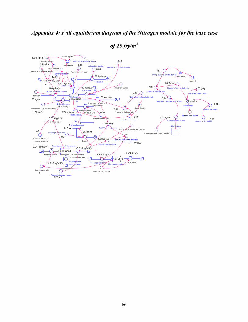
66

Appendix 4: Full equilibrium diagram of the Nitrogen module for the base case

of 25 fry/m2

N in the pond

N concentration in the channel

N of intake water

N f rom f eed

N f rom seed and f ertilizer

Volatization

N in shrimp

Sedimentation


Stock density

Feed applied

Percent of N in f eed

~

f eed by density

N conc in intake water

N remov ed by drainage

to the channel

N remov al drainage rateremineralization

~

sediment remov al rate

Removal by tide




Fry weight

N in f ry

Fertilizer

annual water f low demand per ha

Shrimp land.Start?

Total N discharge mass

N in pond sediment

~

shrimp surv iv al rate by density

dredging remov al rate

~

Shrimp surv iv al rate by N ef f ect

~

sedimination rate

~

drain water sedimentation ratio

Volatization f raction

N in the pond

N concentration in pond


integrated surv iv al rate

Shrimp land.Start?

expected shrimp weight

shrimp y ield

percent of dry weight

Shrimp dry weight


Stock density

N concentration

f rom drainage water

dredging


Shrimp?

Tidal remov al

Shrimp dry weight


remineralization rate

~

tidal remov al rate

Stock density

~

Shrimp land.Total effective

shrimp land

Channel estimated v olume

N concentration

f rom upstream

total discharge v olume

~

shrimp survival rate by density

discharge sediment

48 kg/ha/yr

33 kg/ha/yr

60 kg/ha/yr

156 kg/ha/yr

111 kg/ha/yr

305 kg/ha/yr

227 kg/ha/yr 14 kg/ha/yr

0.11

0.010 kg/m3/yr0.013kg/m3/yr

0.003 kg/m3/yr

1.65E5 kg/yr

555 kg/ha

237 kg

1.65E5 kg

0.013 kg/m3

1

2E6 m3

779 ha

9.35E6 m3

1.22E5 kg

1

213 kg/yr

1.65E5 kg/yr

0.9

0.009 kg/m3

0.3

12000 m3

20 kg/ha

0.07

0.06

4350 kg/ha8700 kg/ha

25 fry/ha

1g/fry

28 kg/ha

0.06

0.41

0.28

0.69

0.05 kg/m3

0.54

0.5

0.27

67239 fry

30 g/fry

2 tons/ha

0.54

0.27

modeling socio-economic and environmental impacts … · 2009-04-29 · vi modeling socio-economic...

Documents