ACPD5, 12697–12722, 2005

Mixing heightdetermination by

ceilometer

N. Eresmaa et al.

Title Page

Abstract Introduction

Conclusions References

Tables Figures

J I

J I

Back Close

Full Screen / Esc

Print Version

Interactive Discussion

EGU

Atmos. Chem. Phys. Discuss., 5, 12697–12722, 2005www.atmos-chem-phys.org/acpd/5/12697/SRef-ID: 1680-7375/acpd/2005-5-12697European Geosciences Union

AtmosphericChemistry

and PhysicsDiscussions

Mixing height determination by ceilometer

N. Eresmaa1, A. Karppinen1, S. M. Joffre1, J. Rasanen2, and H. Talvitie2

1Finnish Meteorological Institute, Research and Development, Helsinki, Finland2Vaisala Oyj, Vantaa, Finland

Received: 30 September 2005 – Accepted: 16 November 2005 – Published: 9 December2005

Correspondence to: A. Karppinen (ari.karppinen@fmi.fi)

© 2005 Author(s). This work is licensed under a Creative Commons License.

12697

ACPD5, 12697–12722, 2005

Mixing heightdetermination by

ceilometer

N. Eresmaa et al.

Title Page

Abstract Introduction

Conclusions References

Tables Figures

J I

J I

Back Close

Full Screen / Esc

Print Version

Interactive Discussion

EGU

Abstract

A novel method for estimating the mixing height based on ceilometer measurements isdescribed and tested against commonly used methods for determining mixing height.In this method an idealised backscatter profile is fitted to the observed backscatterprofile. The mixing height is one of the idealised backscatter profile parameters.5

An extensive amount of ceilometer data and vertical soundings data from the Helsinkiarea in 2002 is utilized to test the applicability of the ceilometer for mixing height deter-mination. The results, including 71 convective and 38 stable cases, show that in clearsky conditions the mixing heights determined from ceilometer based aerosol profilesand BL–height estimates based on sounding data are in a good agreement. Rejected10

outlier cases corresponded to very low aerosol concentrations in the mixed layer lead-ing to a very weak aerosol backscatter signal in the lowest layer.

1. Introduction

The planetary boundary layer (PBL) is the layer where the earth’s surface interactswith the large scale atmospheric flow. Since substances emitted into this layer disperse15

gradually horizontally and vertically through the action of turbulence, and become com-pletely mixed if sufficient time is given and in the absence of sinks or sources, this layeralso called the mixing layer (Seibert et al., 1998).

The PBL height or mixing height (MH) is a key parameter in air pollution modelsdetermining the volume available for pollutants to dispersion (Seibert et al., 2000) and20

the structure of turbulence in the boundary layer (Hashmonay et al., 1991). In spiteof its importance there is no direct method available to determine the MH. The mostcommon methods for determining the MH are utilisation of radiosoundings, remotesounding systems and parameterization methods. All these methods have advantagesand disadvantages and consider different related or assumed properties of the PBL.25

Thus, it is relevant to develop and evaluate new techniques or methods in order to

12698

ACPD5, 12697–12722, 2005

Mixing heightdetermination by

ceilometer

N. Eresmaa et al.

Title Page

Abstract Introduction

Conclusions References

Tables Figures

J I

J I

Back Close

Full Screen / Esc

Print Version

Interactive Discussion

EGU

lower the inherent uncertainty involved in the determination of the MH.Among novel remote sensing methods, a promising one is the ceilometer, based on

the lidar-technique, which measures the aerosol concentration profile. Since in generalaerosol concentrations are lower in the free atmosphere than in the mixing layer wheremost sources of aerosols are located, it can be expected that MH is associated with a5

strong gradient in the vertical back-scattering profile.The objective of this work was to examine the potential of a ceilometer in determining

the mixing height in clear sky conditions. The reference mixing height was determinedutilizing Radiosoundings, several diagnostic formulas for MH and the predictions of ameteorological preprocessor model MetPP-FMI.10

2. Data and techniques

The data used in this work were obtained at the premises of Vaisala Oyj, Vantaa ,Finland, during one year period 5 December 2001–10 November 2002.

2.1. Measurements

2.1.1. Ceilometer15

The Vaisala single-lens ceilometer CT25K (Vaisala Oyj, 2002; Emeis et al, 2004) mea-sures the optical backscatter intensity of the air at a wavelength of 905 nm (near in-frared). Its laser diodes are pulsed with a repetition rate of 5.57 kHz. The lens hasa focal length of 377 mm and an effective diameter of 145 mm. Laser beam full di-vergence and field-of-view divergence of the receiver are 1.4 mrad each. Because of20

the monostatic optical system and the small divergence multiple scattering effects arenegligible and the Mie scattering with scattering angles between 179.9◦ and 180.1◦ isdominant. Additional technical characteristics are given in Table 1.

The CT25K samples the return signal every 100 ns from 0 to 50µs, providing a spa-tial resolution of 15 m from the ground up to an altitude of 7500 m (Vaisala Oyj, 2002).25

12699

ACPD5, 12697–12722, 2005

Mixing heightdetermination by

ceilometer

N. Eresmaa et al.

Title Page

Abstract Introduction

Conclusions References

Tables Figures

J I

J I

Back Close

Full Screen / Esc

Print Version

Interactive Discussion

EGU

For safety and economic reasons, the laser power used is so low that the noise ex-ceeds the backscattering signal. This can be overcome by summing a large number ofreturn signals, so the desired signal will be multiplied by the number of pulses, whereasthe noise, being random, will partially cancel itself. The degree of cancellation for white(Gaussian) noise equals the square root of the number of samples. However, this5

processing gain cannot be extended ad infinitum since the environment is constantlychanging.

The backscatter intensity depends mainly on the particulate concentrations in the air.As the size of particles varies with their moisture content, the reflectivity is influencedby atmospheric humidity, too. Clouds, fog and precipitation inhibit measurements. The10

performance of the CT25K ceilometer is sufficient for analysing boundary-layer struc-tures. Compared to more sophisticated LIDAR systems commonly used for these in-vestigations it has several advantages, including the low first range gate, its ability tooperate eye-safe and maintenance-free for several years in any climatic environmentwith just some regular window cleaning, and its comparably low price. Main disadvan-15

tage due to the low emitted power is its relatively low maximum range, but for mixinglayer studies (mostly below 3 km) this does not present a problem.

Raw ceilometer profiles were obtained every 15 s (integrated over 65 536 individ-ual pulses). For this study, the original ceilometer data were averaged over period of30 min.20

2.1.2. Radiosoundings

The reference mixing height was determined from the analysis of radiosoundings.Soundings were performed regularly during the observation period, mainly duringworking hours. The launching site was 100 m from the ceilometer. However, due tofrequent cloudiness at the study site, a large amount of the soundings had to be re-25

jected. The remaining 109 soundings were divided into convective (N=71) and stable(N=38) cases.

12700

ACPD5, 12697–12722, 2005

Mixing heightdetermination by

ceilometer

N. Eresmaa et al.

Title Page

Abstract Introduction

Conclusions References

Tables Figures

J I

J I

Back Close

Full Screen / Esc

Print Version

Interactive Discussion

EGU

2.2. Method for estimating the mixing height from ceilometer measurements

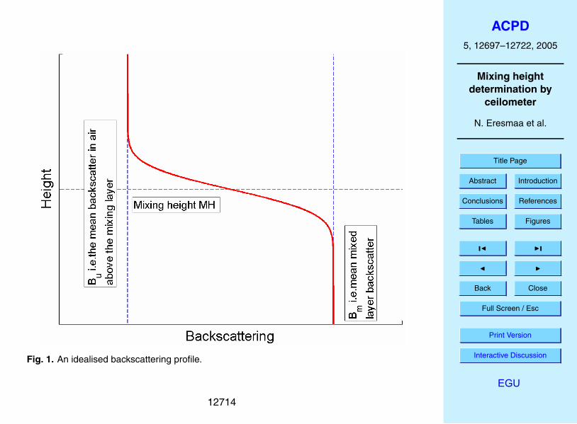
The mixing height h was determined from the backscattering profile using the methoddescribed by Steyn et al. (1999). In this method an idealized backscattering profile B(z)is fitted to measured profile by the formula

B(z) =Bm + Bu

2−

Bm − Bu

2erf

(z − h∆h

)(1)

5

where Bm is the mean mixing layer backscatter, Bu is the mean backscatter in air abovethe mixing layer and ∆h is related to the thickness of the entrainment layer capping thePBL in convective conditions.

We define new constants A1 and A2 so that A1=(Bm+Bu)/2 and A2=(Bm−Bu)/2. Anidealised profile structure corresponding Eq. (1) is illustrated in Fig. 1. In this idealised10

case the backscatter above mixing layer and inside mixing layer have constant valuesBu and BM correspondingly and MH is defined to be the height of the centre of theentrainment layer.

The fitting procedure was automated with Matlab 7.0 software package (Math WorksInc.). The parameter A1 in Eq. (1) is kept fixed during the fitting. However, the fitting is15

strongly dependent on the initial values; therefore it is more efficient if these values arechosen according to the initial order-of-magnitude estimate for the mixing height basedon stability conditions and the structure of the backscattering profile.

If the mixing height is initially estimated to be low (less than 700 m), A1 is chosen tobe the backscattering intensity near the surface. Otherwise A1 is defined as the mean20

backscattering intensity within the mixing layer. In such a case, a running mean is alsoused for smoothing the backscattering profile.

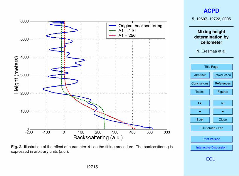
The effect of the choice of initial values (mainly A1) on an actual profile fitting isshown in Fig. 2. This case displays a strong gradient near the surface, topped bya layer of nearly constant backscattering. Another strong gradient can be observed25

at the top of the convective mixing layer (ca. 2000 m). If the value of A1 is chosenerroneously based on the lowest strong gradient (A1=250), the resulting mixing height

12701

ACPD5, 12697–12722, 2005

Mixing heightdetermination by

ceilometer

N. Eresmaa et al.

Title Page

Abstract Introduction

Conclusions References

Tables Figures

J I

J I

Back Close

Full Screen / Esc

Print Version

Interactive Discussion

EGU

is too low, around 1000 m. If the choice of A1 is based on the second strong gradientcorresponding to the mean backscattering in the layer below 2000 m (A1=110), alsothe mixing height is determined correctly to be ca. 1600 m.

Though the ceilometer can observe the atmosphere up to 7500 m, it is not relevantto use the whole backscattering profile due to the strong white noise above 4000 m.5

Therefore, the maximum height of the used profile was set at 4500 m, but if the initialmixing height was lower than 1500 m, only the first 3000 m of backscattering profilewas used.

2.3. Determination of the reference mixing height

2.3.1. Mixing height based on radiosoundings10

In convective situations, the MH was estimated from radiosounding temperature pro-files using the Holzworth-method (Holzworth, 1964, 1967). Its principle is to follow thedry adiabatic starting at the surface up to its intersection with the actual temperatureprofile (Fig. 3). Thus, the method determines the maximum mixing height. This methoddepends strongly on the surface temperature (Seibert et al., 2000), and a high uncer-15

tainty may occur in a situation without a clear inversion at the convective boundarylayer top.

In stable situations, the Richardson number Ri method has traditionally been usedfor determining the mixing height (Vogelezang and Holtslag, 1996). This method deter-mines the equilibrium mixing height rather than the actual mixing height (Zilitinkevich20

and Baklanov, 2002) since the MH h is identified as the level where Ri is equal or largerthan a pre-fixed critical value. Thus, its accuracy is not very high, but the MH is not welldefined either due to low and gradually decreasing turbulence intensity with height. Inthis project the Richardson number profile was determined by the formula of Joffre etal. (2001), which aims at smoothing out some of the inherent fluctuations (especially of25

12702

ACPD5, 12697–12722, 2005

Mixing heightdetermination by

ceilometer

N. Eresmaa et al.

Title Page

Abstract Introduction

Conclusions References

Tables Figures

J I

J I

Back Close

Full Screen / Esc

Print Version

Interactive Discussion

EGU

wind) between adjacent layers:

Ri (zi+1) =gTs

(θi+2 − θi ) (zi+2 − zi )

(Vi+2 − Vi )2

(2)

where Ts is the near-surface air temperature, θi the potential temperature and Vi thewind speed at corresponding level zi . The sub-index i refers to the number of the layerof the profile.5

Though the traditional value of the critical Ri-number is 0.25, there is evidence thatit actually depends on various external conditions such as roughness and free flowstability or the Brunt-Vaisala frequency (Zilitinkevich and Baklanov, 2002). Severalstudies have found better fits with higher Ri-values, in general in connection with alarger-scale approach (Joffre, 1981; Maryon and Best, 1992). The critical value used10

here was 1.0. Figure 4 displays an example of an observed Ri-profile in Vantaa.In absence of wind profile data, the reference mixing height was determined in three

different ways using the sole temperature profile. In method 1, the MH was determinedas the height of the surface inversion (Fig. 5a). In method 2, the MH was determined asthe lowest level at which the virtual potential temperature begins to stray significantly15

from a linear profile (Wetzel, 1982; Fig. 5b). Under conditions of strong winds thepotential temperature increases only slightly in the mixing layer (Zeman, 1979; Fig. 5c).This layer is capped by a quite shallow zone with a very sharp increase in temperature(Seibert et al., 1998). If the MH can be determined in more than one way, the averageis used.20

2.3.2. Mixing height estimated by the meteorological model MetPP-FMI

The mixing height was also determined using the preprocessor model MetPP-FMI(Karppinen et al., 1997). The details of the mixing height scheme can be obtainedfrom Karppinen et al. (1998) and Seibert et al. (2000). The evaluation of the boundarylayer height is based upon routine radiosounding data. The model utilizes the midday25

(12:00 UTC) and midnight (00:00 UTC) soundings. Its main principles are that, under12703

ACPD5, 12697–12722, 2005

Mixing heightdetermination by

ceilometer

N. Eresmaa et al.

Title Page

Abstract Introduction

Conclusions References

Tables Figures

J I

J I

Back Close

Full Screen / Esc

Print Version

Interactive Discussion

EGU

stable and neutral conditions, the MH is proportional to the friction velocity determinedfrom the wind profile following the Monin-Obukhov similarity theory and to the heat fluxintegral (accumulated heat) as determined by the temperature difference between twosubsequent profiles. Under unstable conditions, the MH is determined from the Ten-nekes (1973) model utilizing the measured temperature profiles and modelled stability5

parameters.

2.3.3. Diagnostic methods for determining mixing height in stable situations

In stable situations the mixing height is determined using three different diagnosticmethods. The first method used is a heuristic model for the mixing height derived byJoffre and Kangas (2001):10

h = CstL3/4N L1/4 (3)

where Cst=7.71 is an empirical constant, L is the Monin-Obukhov length and LN=u∗/N,where u∗ is the friction velocity and N the Brunt-Vaisala frequency, which is determinedfrom the radiosonde temperature profiles on a 200 m thick layer about 100 m above themixing layer.15

The Monin-Obukhov-length L and the friction velocity u∗ are determined iterativelyfrom the two lowest radiosounding observations (approximately 5 and 15 m). It is clearthat due to the known strong flings of the balloon in the first seconds of the sound-ing and to the sub-urban environment (heterogeneity), these estimates of u∗ are veryuncertain and results should be considered with care.20

The second method determines the MH based on the classical neutral formula in-volving the friction velocity u∗ and the Coriolis-parameter f (Rossby and Montgomery,1935)

h = au∗f

(4)

12704

ACPD5, 12697–12722, 2005

Mixing heightdetermination by

ceilometer

N. Eresmaa et al.

Title Page

Abstract Introduction

Conclusions References

Tables Figures

J I

J I

Back Close

Full Screen / Esc

Print Version

Interactive Discussion

EGU

The proposed values for the empirical constant a are scattered in the range of a=0.05–0.3. Here we have used the value a=0.14, corresponding roughly to the median of thevalues presented in literature and also coinciding with the value presented by Arya(1981) based on sodar data.

The third method is a classical approximation for the height of the stable Ekman-layer5

(Zilitinkevich, 1972)

h = Bs

√Lu∗f

(5)

We have used value Bs=2 for the empirical proportionality constant according to theoriginal Zilintiekevich (1972) estimate.

3. Results and discussion10

We present here the results of the comparison of ceilometer derived MH values withradiosounding estimates and various parametrisation scheme values. The analysisis performed separately for convective and stable conditions. This multi-estimate ap-proach is partly driven by both the fuzziness of the MH concept and the inherent limi-tations of each single model or method.15

3.1. Convective situations

The comparison between MH values estimated by the ceilometer and those from ra-diosoundings is shown in Fig. 6. A total of 71 clear sky cases were analysed. Fifteenobservations were tagged and rejected from the statistical analysis because they rep-resented low backscattering signal conditions near the surface. A regression line was20

fitted to the remaining 56 observations (blue dots) yielding:

hceilometer = (0.80 ± 0.10)hsounding + (47 ± 89) (6)

12705

ACPD5, 12697–12722, 2005

Mixing heightdetermination by

ceilometer

N. Eresmaa et al.

Title Page

Abstract Introduction

Conclusions References

Tables Figures

J I

J I

Back Close

Full Screen / Esc

Print Version

Interactive Discussion

EGU

The correlation between the MH-estimates of these two methods is very significant(r=0.90; t=15.2; p<0.0001). Thus, the mixing heights predicted by the ceilometeragree well with the mixing heights determined by the parcel method. However, thisholds true only for the situations where the aerosol concentrations are high enough toprovide reliable backscatter profiles, this method can not provide information on the5

MH if the backscatter signal near the surface is too low (red dots in Fig. 6).On the average, the mixing height determined from radiosoundings is 8% higher

than the one determined by the ceilometer. This difference is rather small in spite ofthe fact that these two methods differ in the physical definition of the mixing height.The Holzworth-method determines the maximum height of mixing from the potential10

temperature profile, while the ceilometer “feels” the height at which the aerosol pro-file reaches the edge of the mixing layer (with the implied assumption that aerosolare scarcer above the MH). Thus, at least qualitatively, this observed difference has areasonable physical explanation.

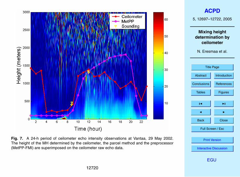
An example of a full 24-h period of ceilometer observations is displayed in Fig. 7.15

It can be easily seen how turbulence gets stronger and the MH grows as the sunrises. On the other hand, the unrealistically high MH values during night time (01:00–03:00 a.m.) provide a good illustration of a potential problem using this method oper-ationally. In this case the algorithm used for obtaining the initial values of the profilefitting procedure leads to erroneous result, as the night time residual aerosol layer is20

interpreted as the real mixed layer. Although this kind of misinterpretation can be easilyavoided if other meteorological measurements are considered in the MH assessment,further work is still required to achieve a completely automatic algorithm for mixingheight determination.

12706

ACPD5, 12697–12722, 2005

Mixing heightdetermination by

ceilometer

N. Eresmaa et al.

Title Page

Abstract Introduction

Conclusions References

Tables Figures

J I

J I

Back Close

Full Screen / Esc

Print Version

Interactive Discussion

EGU

3.2. Stable situations

3.2.1. Comparison of mixing height estimated by the ceilometer and radiosoundings

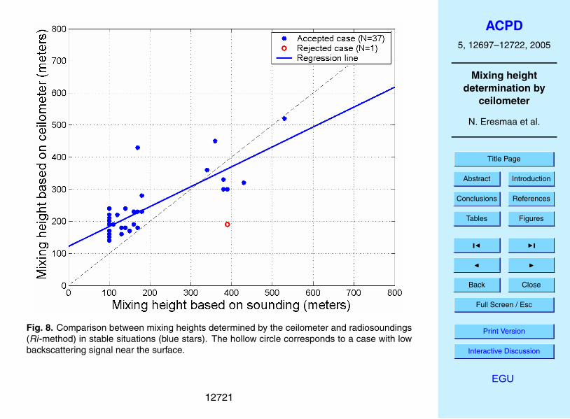
The comparison between the MHs measured by the ceilometer and those estimatedfrom radiosoundings (through the Ri-method) is shown in Fig. 8. A total of 38 clearsky cases were analysed, of which only one was rejected from the statistical analysis5

due to low backscattering signal near the surface. The statistical analysis yielded thefollowing regression line for the remaining 37 observations:

hceilometer = (0.62 ± 0.16)hsounding + (120 ± 34) (7)

The correlation between the two estimates is also in stable case very significant(r=0.80; t=7.9; p<0.0001). On average, the mixing height determined from the sound-10

ing is 25% higher than the one determined by the ceilometer. Thus, the agreement isless than for unstable conditions but this was expected as the height of the MH is lesswell-defined under stable conditions without marked discontinuities in meteorologicaland probably aerosol profiles.

Figure 9 displays a period with a marked surface inversion that occurred on 2–315

January 2002. In case of a cloudy situation the MH determined by the ceilometer iszero. It can easily be seen that the absolute difference between the MHs determinedby the ceilometer, from the soundings and the preprocessor models are not very large,only 100–200 m. The relative difference, however, is much larger since the MH isshallow and at times the MH determined by the ceilometer is 3 times larger than the20

one determined by the preprocessor model.On the basis of all the accepted stable situations, the lowest MH determined by

the ceilometer is 140 m, though estimates from radiosoundings and the preprocessormodel indicate lower mixing heights. This would indicate that the ceilometer methodcannot determine the mixing height in very stable situations, or that the mixing height in25

such situations is higher than soundings and the preprocessor model seem to indicate.This is linked to the unresolved issue of the simulation of strong stable situations in

12707

ACPD5, 12697–12722, 2005

Mixing heightdetermination by

ceilometer

N. Eresmaa et al.

Title Page

Abstract Introduction

Conclusions References

Tables Figures

J I

J I

Back Close

Full Screen / Esc

Print Version

Interactive Discussion

EGU

numerical weather prediction or dispersion models where standard schemes seem toindicate decaying turbulence with as a corollary weak surface fluxes and a shallow MH.On the other hand, scattered data seems to indicate that turbulence and surface fluxescan be sustained by non-local effects. Thus, none of the previous alternatives can beyet favoured.5

3.2.2. Comparison with diagnostic methods in stable situations

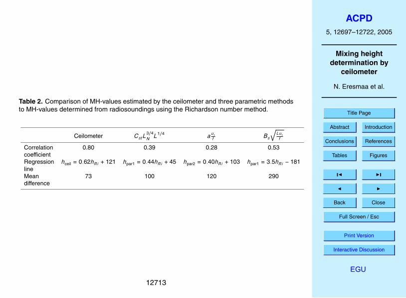
In stable situations, as an additional test, mixing height values estimated from theceilometer and determined by three different parametric methods were compared tothe mixing heights determined from radiosoundings by the Richardson number method(Table 2). The MH based on the Richardson number method acts also here as the10

reference value.The mixing height determined by the ceilometer has clearly the best correlation with

the mixing height determined by the Richardson number method. Also the mean dif-ference between the MHs determined by these two methods is the smallest.

4. Summary and conclusions15

When comparing mixing heights determined by a ceilometer from those by sound-ings, one must remember that these two approaches observe different characteristics.Soundings define the height up to which mixing can happen, while the ceilometer esti-mates the mixing height from the point of view of aerosol profiles. The latter assumesthat aerosols are primarily released from surface sources. On the other hand, aerosols20

can occur at elevated levels originating from distant sources or from the past history ofthe local PBL with a decoupling between the newly developing PBL and the fossil PBL.

Under convective situations, the mixing height determined by the ceilometer cor-relates well with the mixing height determined from radiosoundings with the parcelmethod (the correlation coefficient r=0.90). This can be considered as a reliable result25

12708

ACPD5, 12697–12722, 2005

Mixing heightdetermination by

ceilometer

N. Eresmaa et al.

Title Page

Abstract Introduction

Conclusions References

Tables Figures

J I

J I

Back Close

Full Screen / Esc

Print Version

Interactive Discussion

EGU

due to the large number of observations. There are, however, some differences be-tween these two methods (see Fig. 6) especially in cases of large mixing height whenthe Holzworth method yields larger mixing heights than the ceilometer. This can beexplained, at least qualitatively, from the fact that these two methods define the mixingheight physically in a different way. The Holzworth-method determines the maximum5

height of mixing from the potential temperature profile, while the ceilometer gives theheight where the aerosol profiles indicate the edge of the mixed layer (with the impliedassumption that aerosol are scarcer above the MH).

Under stable situations, there is a good connection between mixing heights deter-mined by the ceilometer and those estimated from soundings with the Ri-method. Even10

if there are fewer observations than in convective situations, this result can also be con-sidered statistically reliable. In very stable situations, the mixing height determined bythe ceilometer is higher than the one determined by parametric methods or estimatedfrom soundings. Reliable conclusions, however, cannot be made because of only afew observations and the uncertainty with regards to turbulence structure and the MH15

under such situations.Nevertheless, this study indicates that a ceilometer can be a suitable instrument for

determining the convective mixing height. However, it cannot be used yet in a fully-automatic mode due to the need to cancel cloudy situations and the possibility of ele-vated aerosol layers outside the PBL. Compared to traditional, operational soundings,20

the advantage of the ceilometer is the possibility of obtaining MH information continu-ously with a very good vertical resolution.

Acknowledgements. The funding from the National Technology Agency of Finland (TEKES)Technology Programme: “FINE Particles – Technology, Environment and Health“ is gratefullyacknowledged.25

12709

ACPD5, 12697–12722, 2005

Mixing heightdetermination by

ceilometer

N. Eresmaa et al.

Title Page

Abstract Introduction

Conclusions References

Tables Figures

J I

J I

Back Close

Full Screen / Esc

Print Version

Interactive Discussion

EGU

References

Arya, S. P. S.: Parameterizing the height of the stable atmospheric boundary layer, J. Appl.Meteorol., 20, 1192–1201, 1981.

Emeis, S., Munkel, C., Vogt, S., Muller, W. J., and Schafer, K.: Atmospheric boundary-layerstructure from simultaneous SODAR, RASS and ceilometer measurements, Atmos. Environ.,5

38, 273–286, 2004.Hashmonay, R., Cohen, A., and Dayan, U.: Lidar observations of atmosphere boundary layer

in Jerusalem, J. Appl. Meteorol., 30, 1228–1236, 1991.Holzworth, C. G.: Estimates of mean maximum mixing depths in the contiguous United States,

Mon. Wea. Rev., 92, 235–242, 1964.10

Holzworth, C. G.: Mixing depths, wind speeds and air pollution potential for selected locationsin the United States, J. Appl. Meteorol., 6, 1039–1044, 1967.

Joffre, S. M.: The Physics of the Mechanically-Driven Atmospheric Boundary Layer as an Ex-ample of Air-Sea Ice Interactions, University of Helsinki, Dept. of Meteorology, Report No.20, 1981.15

Joffre, S. M., Kangas, M., Heikinheimo, M., and Kitaigorodskii, S. A.: Variability of the stable andunstable atmospheric boundary layer height and its scales over a boreal forest, Boundary-Layer Meteorol., 99(3), 429–450, 2001.

Joffre, S. and Kangas, M.: Determination and scaling of the atmospheric boundary layer heightunder various stability conditions over a rough surface, edited by: Rotach, M., Fisher, B.,20

and Piringer, M., COST Action 715 Workshop on Urban Boundary Layer Parameterisations(Zurich, 24–25 May 2001), Office for Official Publications of the European Communities, EUR20355, 111–118, 2002.

Karppinen, A., Joffre, S., and Vaajama, P.: Boundary layer parametrization for Finnish regula-tory dispersion models, Int. J. Environ. Pollut., 8, 557–564, 1997.25

Karppinen, A., Kukkonen, J., Nordlund, G., Rantakrans, E.. and Valkama, I.: A dispersionmodelling system for urban air pollution. Finnish Meteorological Institute, Publications on AirQuality 28, Helsinki, 1998.

Maryon, R. H. and Best, M. J.: NAME, ATMES and the boundary layer problem, UK Met. Office(APR) Turbulence and Diffusion Note, No. 204, 1992.30

Rossby, C. G. and Montgomery, R. B.: The layer of frictional influence in wind and oceancurrents, Pap. Phys. Oceanogr. Meteorol., 3(3), 1–101, 1935.

12710

ACPD5, 12697–12722, 2005

Mixing heightdetermination by

ceilometer

N. Eresmaa et al.

Title Page

Abstract Introduction

Conclusions References

Tables Figures

J I

J I

Back Close

Full Screen / Esc

Print Version

Interactive Discussion

EGU

Seibert, P., Beyrich, F., Gryning, S.-E., Joffre, S., Rasmussen, A., and Tercier, Ph.: Mixingheight determination for dispersion modelling, Report of Working Group 2, in: Harmonizationin the Preprocessing of meteorological data for atmospheric dispersion models, COST Action710, CEC Publication EUR 18195, pp. 145–265, 1998.

Seibert, P., Beyrich, F., Gryning, S.-E., Joffre, S., Rasmussen, A., and Tercier, Ph.: Review and5

Intercomparison of Operational Methods for the Determination of the Mixing Height, Atmos.Environ., 34(7), 1001–1027, 2000.

Steyn, D. G., Baldi, M., and Hoff, R. M.: The detection of mixed layer depth and entrain-ment zone thickness from lidar backscatter profiles, J. Atmos. Ocean. Technol., 16, 953–959,1999.10

Tennekes, H.: A model for the dynamics of the inversion above a convective boundary layer, J.Atmos. Sci., 30, 550–567, 1973.

Vaisala Oyj: Ceilometer CT25K: User’s guide, Vaisala Oyj, Vantaa, 2002.Vogelezang, D. H. P. and Holtslag, A. A. M.: Evolution and model impacts of the alternative

boundary layer formulations, Boundary-Layer Meteorol., 81, 245–269, 1996.15

Wetzel, P. J.: Towards parameterization of the stable boundary layer, J. Appl. Meteorol., 21,7–13, 1982.

Zeman, O.: Parameterization of the dynamics of stable boundary layer and nocturnal jets, J.Atmos Sci., 36, 798–804, 1979.

Zilitinkevich, S. S.: On the determination of the height of the Ekman boundary layer, Boundary-20

Layer Meteorol., 3, 141–145, 1972.Zilitinkevich, S. and Baklanov, A.: Calculation of the height of stable boundary layers in practical

applications, Boundary-Layer Meteorol., 105(3), 389–409, 2002.

12711

ACPD5, 12697–12722, 2005

Mixing heightdetermination by

ceilometer

N. Eresmaa et al.

Title Page

Abstract Introduction

Conclusions References

Tables Figures

J I

J I

Back Close

Full Screen / Esc

Print Version

Interactive Discussion

EGU

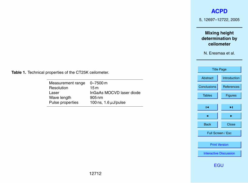
Table 1. Technical properties of the CT25K ceilometer.

Measurement range 0–7500 mResolution 15 mLaser InGaAs MOCVD laser diodeWave length 905 nmPulse properties 100 ns, 1.6µJ/pulse

12712

ACPD5, 12697–12722, 2005

Mixing heightdetermination by

ceilometer

N. Eresmaa et al.

Title Page

Abstract Introduction

Conclusions References

Tables Figures

J I

J I

Back Close

Full Screen / Esc

Print Version

Interactive Discussion

EGU

Table 2. Comparison of MH-values estimated by the ceilometer and three parametric methodsto MH-values determined from radiosoundings using the Richardson number method.

Ceilometer CstL3/4N L1/4 au∗

f Bs

√Lu∗f

Correlation 0.80 0.39 0.28 0.53coefficientRegression hceil = 0.62hRi + 121 hpar1 = 0.44hRi + 45 hpar2 = 0.40hRi + 103 hpar1 = 3.5hRi − 181lineMean 73 100 120 290difference

12713

ACPD5, 12697–12722, 2005

Mixing heightdetermination by

ceilometer

N. Eresmaa et al.

Title Page

Abstract Introduction

Conclusions References

Tables Figures

J I

J I

Back Close

Full Screen / Esc

Print Version

Interactive Discussion

EGU

Fig. 1. An idealised backscattering profile.

12714

ACPD5, 12697–12722, 2005

Mixing heightdetermination by

ceilometer

N. Eresmaa et al.

Title Page

Abstract Introduction

Conclusions References

Tables Figures

J I

J I

Back Close

Full Screen / Esc

Print Version

Interactive Discussion

EGU

Fig. 2. Illustration of the effect of parameter A1 on the fitting procedure. The backscattering isexpressed in arbitrary units (a.u.).

12715

ACPD5, 12697–12722, 2005

Mixing heightdetermination by

ceilometer

N. Eresmaa et al.

Title Page

Abstract Introduction

Conclusions References

Tables Figures

J I

J I

Back Close

Full Screen / Esc

Print Version

Interactive Discussion

EGU

Fig. 3. Illustration of the Holzworth-method. Temperature profile at Vantaa, 29 May 200208:56 UTC.

12716

ACPD5, 12697–12722, 2005

Mixing heightdetermination by

ceilometer

N. Eresmaa et al.

Title Page

Abstract Introduction

Conclusions References

Tables Figures

J I

J I

Back Close

Full Screen / Esc

Print Version

Interactive Discussion

EGU

Fig. 4. An example of the Richardson number profile at Vantaa, 4 January 2002 07:17 UTC.

12717

ACPD5, 12697–12722, 2005

Mixing heightdetermination by

ceilometer

N. Eresmaa et al.

Title Page

Abstract Introduction

Conclusions References

Tables Figures

J I

J I

Back Close

Full Screen / Esc

Print Version

Interactive Discussion

EGU

. Fig. 5. Three ways for determining the reference mixing height from temperature profiles:(a) the height of the surface inversion (5 September 2002 06:06 UTC), (b) virtual potentialtemperature non-linearity (1 February 2002 07:02 UTC) and (c) strong winds – sharp virtualtemperature increase above MH (2 January 2002 06:16 UTC).

12718

ACPD5, 12697–12722, 2005

Mixing heightdetermination by

ceilometer

N. Eresmaa et al.

Title Page

Abstract Introduction

Conclusions References

Tables Figures

J I

J I

Back Close

Full Screen / Esc

Print Version

Interactive Discussion

EGU

Fig. 6. Comparison between mixing heights determined by the ceilometer and radiosoundings(Holzworth method) in convective situations. Data points marked as hollow circles representconditions with low backscattering signal.

12719

ACPD5, 12697–12722, 2005

Mixing heightdetermination by

ceilometer

N. Eresmaa et al.

Title Page

Abstract Introduction

Conclusions References

Tables Figures

J I

J I

Back Close

Full Screen / Esc

Print Version

Interactive Discussion

EGU

Fig. 7. A 24-h period of ceilometer echo intensity observations at Vantaa, 29 May 2002.The height of the MH determined by the ceilometer, the parcel method and the preprocessor(MetPP-FMI) are superimposed on the ceilometer raw echo data.

12720

ACPD5, 12697–12722, 2005

Mixing heightdetermination by

ceilometer

N. Eresmaa et al.

Title Page

Abstract Introduction

Conclusions References

Tables Figures

J I

J I

Back Close

Full Screen / Esc

Print Version

Interactive Discussion

EGU

Fig. 8. Comparison between mixing heights determined by the ceilometer and radiosoundings(Ri-method) in stable situations (blue stars). The hollow circle corresponds to a case with lowbackscattering signal near the surface.

12721

ACPD5, 12697–12722, 2005

Mixing heightdetermination by

ceilometer

N. Eresmaa et al.

Title Page

Abstract Introduction

Conclusions References

Tables Figures

J I

J I

Back Close

Full Screen / Esc

Print Version

Interactive Discussion

EGU

Fig. 9. Mixing height as determined by different methods or schemes during a surface temper-ature inversion (2–3 January 2002).

12722