European cooperation in the field of scientific and technical research

Meteorology

Mixing height and inversionsin urban areas

Proceedings of the workshop

3 - 4 October 2001, Toulouse, France

COST Action 715

European Commission

COST Action 715

Meteorology Applied to Urban Air Pollution Problems

Mixing height and inversionsin urban areas

Proceedings of the workshop

3 - 4 October 2001, Toulouse, France

Edited by:

Martin Piringer

Central Institute for Meteorology and Geodynamics,

Vienna, Austria

and

Jaakko Kukkonen

Finnish Meteorological Institute, Helsinki, Finland

Content

M. Piringer and J. Kukkonen: Introduction 5

Mixing heights

A. Baklanov: The mixing height in urban areas - a review 9

K. Maßmeyer and R. Martens: A recommendation for turbulence parameterisationin German guidelines for the calculation of dispersionin the atmospheric boundary layer – improvements andremaining problems 29

M. Rotach et al.: BUBBLE – current status of the experiment and plannedinvestigation of the urban mixing height 45

F. Said et al.: Influence of sea breeze and relief on the mixing heightduring ESCOMPTE in the Marseille area 53

A. Dandou et al.: Mixing Heights calculations by MM5 and simple pre-processors for atmospheric dispersion modelling 57

Inversions

R. Sokhi et al.: Analysis of Air Pollution Episodes in European Cities 65

E. Berge et al.: Simulations of wintertime inversions in northernEuropean cities by use of NWP-models 75

A. Karppinen: Evaluation of meteorological data measured at a radiotower in the Helsinki Metropolitan Area 89

S. Finardi et al.: Analysis of three air pollution episodes driven by atemperature inversion in a sub-alpine Italian region 99

M. Piringer and J. Kukkonen: Conclusions and recommendations 110

5

Introduction

Martin Piringer1 and Jaakko Kukkonen2

1Central Institute for Meteorology and Geodynamics, Hohe Warte 38, A-1190 Vienna, Austria

e-mail: martin.piringer@zamg.ac.at

2 Finnish Meteorological Institute, Air Quality Research, Sahaajankatu 20 E, FIN–00880

Helsinki, Finland

e-mail: jaakko.kukkonen@fmi.fi

Organisation of the expert meeting

COST-Action 715 held an expert meeting in Toulouse, France, on 3 - 4 October 2001,

comprising of expert presentations on mixing heights and inversions in urban areas. COST is an

acronym of "Co-operation in the fields of Science and Technology", financially supported by the

European Commission to encourage and facilitate mutual scientific exchange among Member

States. Each action is devoted to a specific topic whose main scientific goals are fixed in a so-

called "Memorandum of Understanding", to be signed by COST Member States. An action lasts

in general five years. COST Action 715, chaired by Bernard Fisher, University of Greenwich,

U.K., and Michael Schatzmann, University of Hamburg, Germany, has been signed by

18 countries and will end in September 2003.

COST Action 715 is organised in four working groups, dealing with (1) urban wind fields, (2)

surface energy budget and mixing height, (3) air pollution episodes in cities, and (4)

meteorological input data for urban site studies. The Toulouse workshop was jointly organised by

working groups 2 and 3 that are chaired by the editors of these proceedings.

6

Nine presentations were kept at the meeting in Toulouse, five on mixing heights, four on

inversions. This volume contains the extended abstracts in the temporal order of the presentations

kept at the meeting. The outcome of the general discussions is reflected in the conclusions that

are presented at the end of these proceedings.

The session on mixing heights

Methods for the evaluation of mixing height were reviewed by A. Baklanov. In numerical

weather prediction, the simple closure models do not work well. Nocturnal stable air in urban

areas presents greatest difficulty for modellers. The performance of methods seems more

acceptable in daytime than night. Inhomogeneity of surface types and thermal properties in a city

should be modelled numerically.

R. Martens reviewed German regulatory models: a traditional Gaussian plume model and a new

Lagrangian model. The latter uses turbulence components and Lagrangian time scales to evaluate

the dispersion. In discussion, the problem of inhomogeneity over an urban surface reappeared.

The presentation of the ongoing experiment called BUBBLE (Basle Urban Boundary Layer

Experiment) by M. Rotach showed the effort to set up a comprehensive network of tower and

surface observations. Lidar, Sodar, wind profiler and tethered balloons were used to investigate

the urban boundary layer in detail over a whole year, also for the purpose of subsequent

numerical modelling.

The report of the recent UBL/ESCOMPTE experiment in the greater Marseilles area by F. Said

described also the use of RASS, O3 and particle Lidars. Real profiles showed often multiple

layering, causing difficulty in detecting the mixing height from the Lidar measurements alone. A.

Dandou tested the mixing height schemes within the meso-scale numerical model MM5 for the

Lombardy area in Northern Italy, including Milan, and compared the results to the Milan

radiosoundings.

7

The session on mixing heights concluded with considerable discussion of how are mixing heights

best measured (e.g., via accumulated pollutants in the air, or by profiles, or by remote sensing)

and what is really meant by them. In the context of numerical weather prediction (NWP), is the

mixing height still a valid concept ? It seems that their practical usefulness in understanding

episodes and in running the simpler types of pollution dispersion model renders the concept of

mixing height useful, despite the agreed absence of precision in its definition.

The session on temperature inversions and air quality episodes

R. Sokhi presented the analysis and evaluation of air pollution episodes in several European

cities. Examples of episodes of PM10, NO2 and O3 were presented and the causes were examined

in relation to local emissions and meteorological conditions. For both particulate matter and

nitrogen oxides, low lying inversion and local low wind speeds are particularly important in that

they tend to lead to high concentration of air pollutants. In case of PM10 episodes, resuspended

particulate matter from street surfaces can also be important, especially in Northern and Central

European cities.

E. Berge presented results from NWP modeling in Northern Europe during strong wintertime

inversions, and discussed how realistic these simulations are. Air quality problems in Northern

Europe are often linked to episodes of strong inversions, and high levels of air pollutants such as

NO2 and particulate matter (PM2.5 or PM10) often occur during such events. He utilised numerical

results produced by two NWP models (HIRLAM and ECMWF), combined with the utilisation of

the non-hydrostatic MM5 model. The numerical runs for Oslo using 10, 3 and 1 km nesting

revealed the necessity of high resolution for resolving topographical features. He also simulated

an episode in Helsinki that involved an extremely strong ground-based temperature inversion,

and compared the predicted results with those measured at a radio tower of Kivenlahti.

A. Karppinen evaluated the meteorological data measured at a radio tower of 327 m height,

called the Kivenlahti mast, situated in the Helsinki Metropolitan Area. The archived data contains

wind speed and direction, ambient temperature and relative humidity values, since 1989.

However, the data extracted from such measurements needs to be carefully evaluated in order to

8

find out possible disturbances caused by the presence of the tower itself. The data has been

utilised in evaluating the temporal evolution of temperature inversions in the course of episodes.

As an example, the temperature profiles measured at the mast during 27-28 December 1995

showed a maximum vertical inversion of approximately 15˚C over the lowest 30 m of the

atmosphere.

S. Finardi analysed three different episodes that occurred in cities of Northern Italy. These

episodes were analysed based on synoptic meteorological information, local vertical profiles

from soundings, and meteorological and chemical measurements performed at an air quality

network. He showed that Milan is a city where topography plays an important role in winter

inversions. Whilst high pressure may build the inversion, local processes determine the local

wind field near the ground. The lower circulation may be decoupled from the synoptic scale,

being driven by local and mesoscale effects.

Acknowlewgements

We wish to thank the former secretary of the COST 715 action, Mr. Zoltan Dunkel for taking

care of supporting the expenses of the invited non-COST experts. Special thanks are due to the

local organiser Meteo France, for providing good facilities in the city of Toulouse. We also wish

to thank Douglas R. Middleton (UK Meteorological Office) for allowing us to utilise his

previously written nice overview of this expert meeting. Finally, we express our thanks to all the

speakers for their contributions and to the members of the working groups for helping us to

organise this successful meeting.

9

The mixing height in urban areas - a review

Alexander Baklanov∗

∗ Danish Meteorological Institute (DMI), Lyngbyvej 100, DK-2100 Copenhagen, DENMARK,e-mail: alb@dmi.dk

AbstractThe urban boundary layer (UBL), in comparison with ‘rural’ homogeneous PBLs, ischaracterised by greatly enhanced mixing, resulting from both the large surface roughnessand increased surface heating, and by horizontal inhomogeneity of the mixing height (MH)and other meteorological fields due to variations in surface roughness and heating from ruralto central city areas. So, it is reasonable to consider the UBL as a specific case of theatmospheric boundary layer over a non-homogeneous terrain. Most of the parameterisationsof MH were developed for the conditions of a homogeneous terrain, so their applicability forurban conditions should be verified. Just a few authors suggested specific methods for MHdetermination in urban areas. Some authors tested the applicability of MH methods forspecific urban sites, but a comprehensive analysis of the applicability does not exist yet.Proceeding from analysis of different methods of the MH estimation for urban areas, thefollowing preliminary suggestions are discussed. For the estimation of the daytime MH, theapplicability of common methods is more acceptable than for the nocturnal MH. For theconvective UBL the simple slab models were found to perform quite well. The formation of thenocturnal UBL occurs in a counteraction with the negative ‘non-urban’ surface heat fluxesand positive anthropogenic/urban heat fluxes, so the applicability of the common methods forthe SBL estimation is less promising. Applicability of some newly developed methods for theSBL height estimation, including diagnostic and prognostic equations and an improved Ri-method are also discussed.

Keywords:Urban boundary layer, atmospheric stratification, urban canopy, internal boundary layer,dispersion models.

1. IntroductionMost of the urban atmospheric pollution models request the height of the mixing layer (MH)as input information. Despite the progress in numerical turbulent modelling during the lastdecades, this parameter is still one of the most important ones for correctly forecasting the airquality.However, the mixing height (MH) is not observed by standard measurements, so in dispersionmodels it can be parameterised or obtained from profile measurements or simulations. TheCOST-Action 710 (Fisher et al., 1998) has reviewed different definitions and the practicaldetermination of MH from measurements, by modelling and parameterisation and from outputfrom NWP models. Moreover, it identified and tested pre-processors and computer routines toderive the mixing height and intercompared methods by using several non-urban data sets.During the last decades many experimental studies of the mixing layer were realised for urbanareas. This made it possible to analyse the peculiarities of the urban MH (UMH) and verify(or improve) different methods of the MH estimation versus measurement data sets fromseveral types of urban areas.

So, the follow-up COST-Action 715 develops the scientific work achieved under COST-710from rural to urban conditions. In particular, the Working Group 2 focuses on the specificproblems in describing the surface energy balance and the mixing height in urban areas(Piringer, 2000; Piringer et al., 2001). Within the WMO Global Atmosphere Watchprogramme the Urban Research Meteorology and Environment (GURME) project was alsoinitiated in 1999 (Soudine, 2001).

2. Specificity and features of the urban boundary layerThe urban boundary layer (UBL), in comparison with ‘rural’ homogeneous PBLs, ischaracterised by greatly enhanced mixing, resulting from both the large surface roughness andincreased surface heating, and by horizontal inhomogeneity of the MH and othermeteorological fields due to variations in surface roughness and heating from rural to centralcity areas. So, it is reasonable to consider the UBL as a specific case of the PBL over a non-homogeneous terrain. This relates, first of all, to drastic changes of the surface roughness andurban surface heat fluxes. The scheme of vertical structure of the urban boundary layer can besimplified in the form presented in Figure 1.

As incl

(i) (ii) (iii)(iv)(v)

Figu

a) daytime

PBL IBL UBL ’Urban plume’

Rural Suburb Urban Suburb Rural

b) nocturnal

a result ofuding:

internal urelevated n strong hor so-called anthropoge

re 1: The simprofile

’

Residual layer

PBL IBL UBL ’Urban plume

10

the urban area features there are several aspects for

ban boundary layer (IBL),octurnal inversion layer,izontal inhomogeneity and temporal non-stationarity,

‘urban roughness island’, zero-level of urban canopy, nic heat fluxes from street to city scale,

plified scheme of vertical structure of the urban boundary layers: a) daytime UBL, b) nocturnal UBL.

Rural Suburb Urban Suburb Rural

Rural IBL

analysing the urban MH,

and z0u ≠ z0T,

and typical potential temperature

11

(vi) downwind ‘urban plume’ and scale of urban effects in space and time,(vii) calm weather situation simulation,(viii) non-local character of urban MH formation,(ix) effect of the water vapour fluxes.

3. Experimental studies of Urban Mixing HeightDuring the last decades many experimental studies of the mixing layer in urban areas wererealised (see Table 1). In Northern America comprehensive studies of the urban boundarylayer were done for the Lower Fraser Valley: Vancouver (Stein et al., 1997, Batcharova et al.,1999), Sacramento urban area, California (Cleugh and Grimmon, 2001), Mexico City (Cooperand Eichinger, 1994), St. Louis metropolitan area (Seaman, 1989; Westcott, 1989, Godovichet al, 1987). In Asia urban field experiments were carried out for Beijing and Shenyang citiesin China (Zhang et al., 1991; Sang and Lui, 1990), for the city of Delhi (Kumari, 1985) andJapanese cities (e.g. Chen et al., 2001). For European cities experimental studies of the urbanboundary layer and pollution episodes have already been performed for Basel (Rotach et al.2001), Marseille (Said et al. 2001), Paris (Dupont et al., 1999), Vienna (Piringer et al., 1998)and Graz, Austria (Piringer and Baumann, 1999), Helsinki (Railo, 1997; Karppinen et al.,1998), the valley of Athens (Melas & Kambezidis, 1992; Frank 1997; Kambezidis et al.,1995), Copenhagen (Batcharova & Gryning 1989), Milan (Lena & Desiato, 1999), Sofia(Donev et al., 1995; Kolev et al., 2000), Moscow (Lokoshchenko et al., 1993).

This makes it possible to analyse the effects of the urban peculiarities and to verify differentmethods of the MH estimation versus measurement data sets from several types of urbanareas.

Proceeding from the urban area features discussed above, there are the following importantquestions to answer for analysing the urban MH based on the experimental data:1. How much does the MH in urban areas differ from the rural MH ?2. How does the temporal dynamics of MH in urban areas differ from the rural MH ?3. What is the scale of urban effects in space and time and for how long distance does the

downwind ‘urban plume’ effect the MH ?4. How important is the internal urban boundary layer in forming the MH?

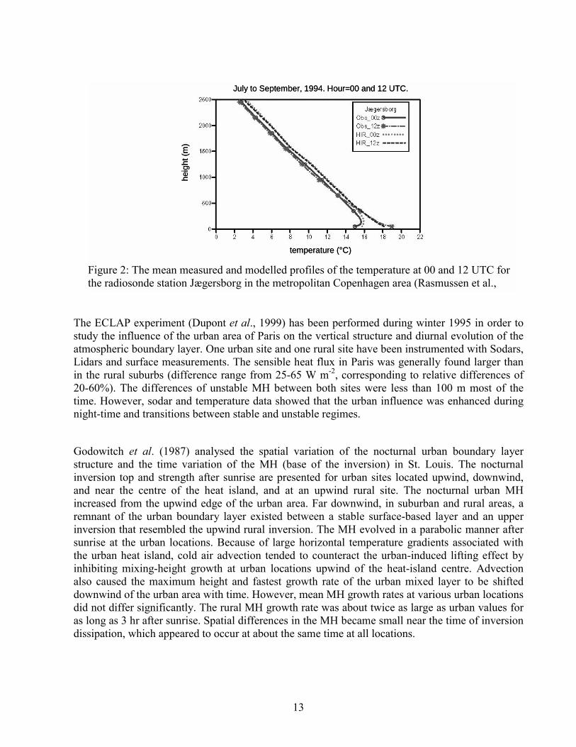
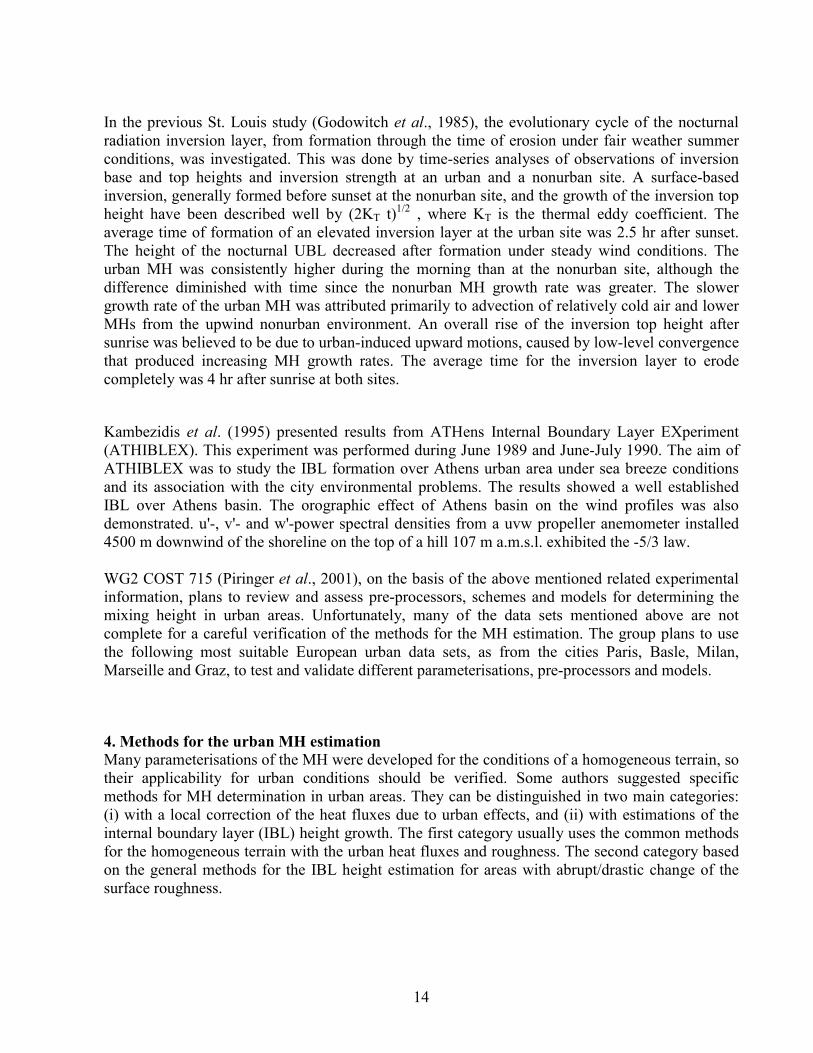
Several experimental studies analysed the difference of MH in urban and rural sites fordifferent geographical regions. There are several geographically different types of cities (e.g.,on a flat terrain or in mountain valleys, coastal area cities, northern or southern cities),peculiarities of each type can affect the forming the urban boundary layer as well. Forexample, the stably stratified nocturnal boundary layer is not common for USA cities(Bornstein, 2001), it could be an elevated nocturnal inversion layer only. However, forEuropean cities, especially in Northern Europe, the nocturnal SBL is very common (e.g., inHelsinki: see Railo, 1997). The mean profiles of the temperature at 00 and 12 UTC for theradiosonde station Jægersborg in Copenhagen (Rasmussen et al., 1999), presented in Figure 2,show clearly the stably stratified nocturnal BL.

12

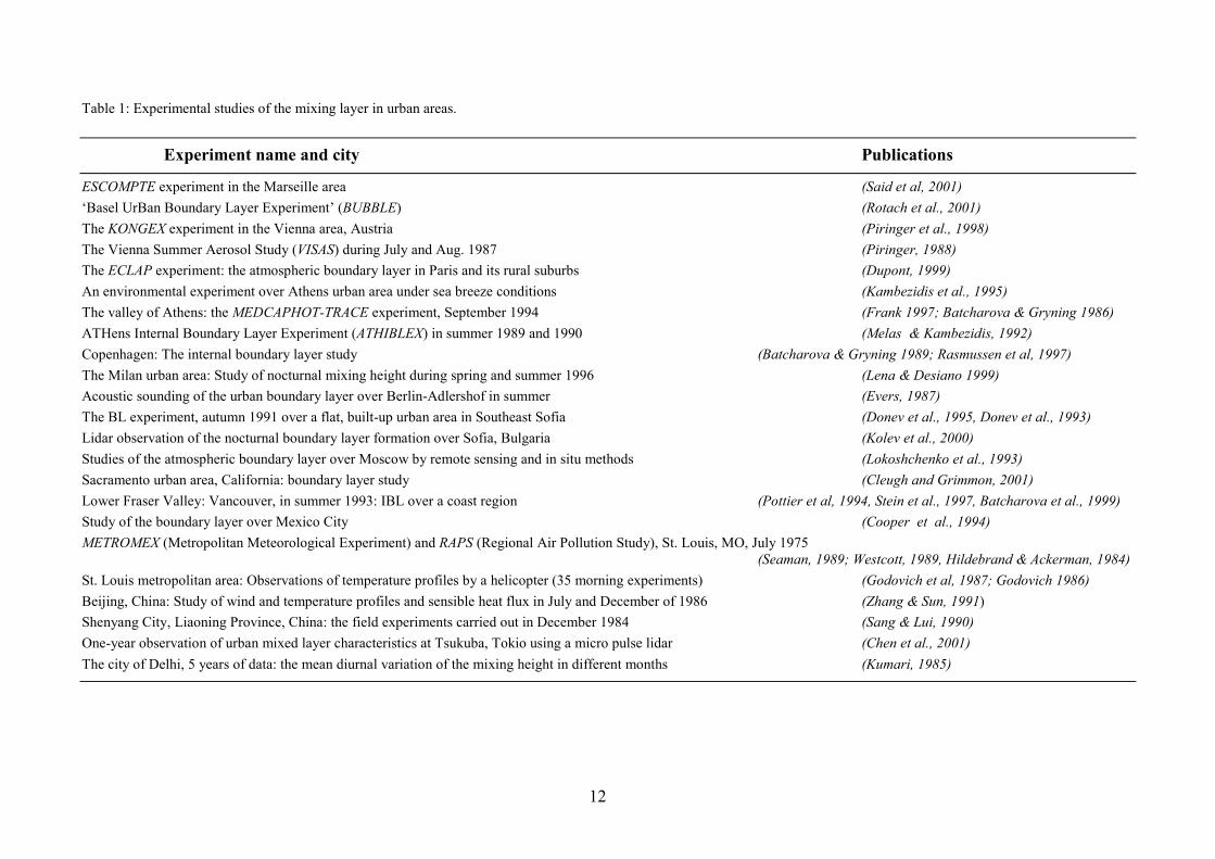
Table 1: Experimental studies of the mixing layer in urban areas.

Experiment name and city Publications

ESCOMPTE experiment in the Marseille area (Said et al, 2001)‘Basel UrBan Boundary Layer Experiment’ (BUBBLE) (Rotach et al., 2001)The KONGEX experiment in the Vienna area, Austria (Piringer et al., 1998)The Vienna Summer Aerosol Study (VISAS) during July and Aug. 1987 (Piringer, 1988)The ECLAP experiment: the atmospheric boundary layer in Paris and its rural suburbs (Dupont, 1999)An environmental experiment over Athens urban area under sea breeze conditions (Kambezidis et al., 1995)The valley of Athens: the MEDCAPHOT-TRACE experiment, September 1994 (Frank 1997; Batcharova & Gryning 1986)ATHens Internal Boundary Layer Experiment (ATHIBLEX) in summer 1989 and 1990 (Melas & Kambezidis, 1992)Copenhagen: The internal boundary layer study (Batcharova & Gryning 1989; Rasmussen et al, 1997)The Milan urban area: Study of nocturnal mixing height during spring and summer 1996 (Lena & Desiano 1999)Acoustic sounding of the urban boundary layer over Berlin-Adlershof in summer (Evers, 1987)The BL experiment, autumn 1991 over a flat, built-up urban area in Southeast Sofia (Donev et al., 1995, Donev et al., 1993)Lidar observation of the nocturnal boundary layer formation over Sofia, Bulgaria (Kolev et al., 2000)Studies of the atmospheric boundary layer over Moscow by remote sensing and in situ methods (Lokoshchenko et al., 1993)Sacramento urban area, California: boundary layer study (Cleugh and Grimmon, 2001)Lower Fraser Valley: Vancouver, in summer 1993: IBL over a coast region (Pottier et al, 1994, Stein et al., 1997, Batcharova et al., 1999)Study of the boundary layer over Mexico City (Cooper et al., 1994)METROMEX (Metropolitan Meteorological Experiment) and RAPS (Regional Air Pollution Study), St. Louis, MO, July 1975

(Seaman, 1989; Westcott, 1989, Hildebrand & Ackerman, 1984)St. Louis metropolitan area: Observations of temperature profiles by a helicopter (35 morning experiments) (Godovich et al, 1987; Godovich 1986)Beijing, China: Study of wind and temperature profiles and sensible heat flux in July and December of 1986 (Zhang & Sun, 1991)Shenyang City, Liaoning Province, China: the field experiments carried out in December 1984 (Sang & Lui, 1990)One-year observation of urban mixed layer characteristics at Tsukuba, Tokio using a micro pulse lidar (Chen et al., 2001)The city of Delhi, 5 years of data: the mean diurnal variation of the mixing height in different months (Kumari, 1985)

13

The ECLAP experiment (Dupont et al., 1999) has been performed during winter 1995 in order tostudy the influence of the urban area of Paris on the vertical structure and diurnal evolution of theatmospheric boundary layer. One urban site and one rural site have been instrumented with Sodars,Lidars and surface measurements. The sensible heat flux in Paris was generally found larger thanin the rural suburbs (difference range from 25-65 W m-2, corresponding to relative differences of20-60%). The differences of unstable MH between both sites were less than 100 m most of thetime. However, sodar and temperature data showed that the urban influence was enhanced duringnight-time and transitions between stable and unstable regimes.

Godowitch et al. (1987) analysed the spatial variation of the nocturnal urban boundary layerstructure and the time variation of the MH (base of the inversion) in St. Louis. The nocturnalinversion top and strength after sunrise are presented for urban sites located upwind, downwind,and near the centre of the heat island, and at an upwind rural site. The nocturnal urban MHincreased from the upwind edge of the urban area. Far downwind, in suburban and rural areas, aremnant of the urban boundary layer existed between a stable surface-based layer and an upperinversion that resembled the upwind rural inversion. The MH evolved in a parabolic manner aftersunrise at the urban locations. Because of large horizontal temperature gradients associated withthe urban heat island, cold air advection tended to counteract the urban-induced lifting effect byinhibiting mixing-height growth at urban locations upwind of the heat-island centre. Advectionalso caused the maximum height and fastest growth rate of the urban mixed layer to be shifteddownwind of the urban area with time. However, mean MH growth rates at various urban locationsdid not differ significantly. The rural MH growth rate was about twice as large as urban values foras long as 3 hr after sunrise. Spatial differences in the MH became small near the time of inversiondissipation, which appeared to occur at about the same time at all locations.

temperature (°C)

heig

ht (m

)

July to September, 1994. Hour=00 and 12 UTC.

temperature (°C)

heig

ht (m

)

July to September, 1994. Hour=00 and 12 UTC.

Figure 2: The mean measured and modelled profiles of the temperature at 00 and 12 UTC forthe radiosonde station Jægersborg in the metropolitan Copenhagen area (Rasmussen et al.,

)

14

In the previous St. Louis study (Godowitch et al., 1985), the evolutionary cycle of the nocturnalradiation inversion layer, from formation through the time of erosion under fair weather summerconditions, was investigated. This was done by time-series analyses of observations of inversionbase and top heights and inversion strength at an urban and a nonurban site. A surface-basedinversion, generally formed before sunset at the nonurban site, and the growth of the inversion topheight have been described well by (2KT t)1/2 , where KT is the thermal eddy coefficient. Theaverage time of formation of an elevated inversion layer at the urban site was 2.5 hr after sunset.The height of the nocturnal UBL decreased after formation under steady wind conditions. Theurban MH was consistently higher during the morning than at the nonurban site, although thedifference diminished with time since the nonurban MH growth rate was greater. The slowergrowth rate of the urban MH was attributed primarily to advection of relatively cold air and lowerMHs from the upwind nonurban environment. An overall rise of the inversion top height aftersunrise was believed to be due to urban-induced upward motions, caused by low-level convergencethat produced increasing MH growth rates. The average time for the inversion layer to erodecompletely was 4 hr after sunrise at both sites.

Kambezidis et al. (1995) presented results from ATHens Internal Boundary Layer EXperiment(ATHIBLEX). This experiment was performed during June 1989 and June-July 1990. The aim ofATHIBLEX was to study the IBL formation over Athens urban area under sea breeze conditionsand its association with the city environmental problems. The results showed a well establishedIBL over Athens basin. The orographic effect of Athens basin on the wind profiles was alsodemonstrated. u'-, v'- and w'-power spectral densities from a uvw propeller anemometer installed4500 m downwind of the shoreline on the top of a hill 107 m a.m.s.l. exhibited the -5/3 law.

WG2 COST 715 (Piringer et al., 2001), on the basis of the above mentioned related experimentalinformation, plans to review and assess pre-processors, schemes and models for determining themixing height in urban areas. Unfortunately, many of the data sets mentioned above are notcomplete for a careful verification of the methods for the MH estimation. The group plans to usethe following most suitable European urban data sets, as from the cities Paris, Basle, Milan,Marseille and Graz, to test and validate different parameterisations, pre-processors and models.

4. Methods for the urban MH estimationMany parameterisations of the MH were developed for the conditions of a homogeneous terrain, sotheir applicability for urban conditions should be verified. Some authors suggested specificmethods for MH determination in urban areas. They can be distinguished in two main categories:(i) with a local correction of the heat fluxes due to urban effects, and (ii) with estimations of theinternal boundary layer (IBL) height growth. The first category usually uses the common methodsfor the homogeneous terrain with the urban heat fluxes and roughness. The second category basedon the general methods for the IBL height estimation for areas with abrupt/drastic change of thesurface roughness.

15

4.1. Estimation of the MH or eddy profile from meteorological modelsOne of the promising methods to estimate the MH or the eddy profile for dispersion models isusing output from numerical meso-meteorological or weather prediction (NWP) models. Severalpossible ways are used in different publications.First of all, it is possible to avoid the usage of the MH for dispersion models, which can directlyuse the eddy diffusivity profiles. Many advanced atmospheric dynamics and pollution modelsalready follow this way (e.g., Baklanov, 2000a; Zhang et al., 2001; Kurbatskii, 2001). However,many models, especially regulatory models, are not coupled with meteorological models. They arebased on in situ measurements of meteorological characteristics and need the MH as an inputparameter.Some meteorological models calculate the planetary boundary layer (PBL) height and then use itas the height of the simulation area. Such models were suggested by Penenko and Aloyan (1974,1985). A simple version of this method was also realised by Arya & Byun (1987) and Byun &Arya (1990) for a 2-D numerical model of the urban BL. Such a method can be very useful fornext-generation models, especially if meteorological models include the urban effects. However,such models are much more expensive in computation time.

During the last years, output data from 3-D NWP models were increasingly used for MHestimation based on different approaches, e.g.: turbulent kinetic energy models, k-ε models,subgrid scale turbulent closure models (incl. LES mode), second momentum turbulent closuremodels. The MH can be estimated from vertical profile of meteorological fields, e.g. based on:• turbulent kinetic energy or eddy decay/depletion,• Richardson-number method,• different parameterisations and simple models. Direct calculations of the MH from simulated turbulent kinetic energy or eddy profiles (so-calledturbulent kinetic energy or eddy decay method) for the daytime urban boundary layers showedgood and promising results (see e.g., Batchwarova et al., 1999). However, this way is verysensitive to the turbulent closure scheme, so it can be quite dangerous for practical use. E.g., Zhanget al. (2001) showed that local closure schemes gave considerable errors for the daytime MH aswell. In spite of promising results for the CBL height, use of this method for the nocturnal MH(stably stratified BL) can give considerable problems and large uncertainties for the MHestimation, e.g. from TKE equations with a local closure. For example, a new version of the DMI-HIRLAM model (Saas et al., 2000; Nielsen and Saas, 2000) with the CBR turbulence scheme(Cuxard et al., 2000) tested a direct calculation of the PBL height from the turbulent energy profileby the TKE depletion approach. However, it was shown (Baklanov, 2000b) that this method givesa considerable underestimation of the height of the nocturnal PBL.

4.2. Applicability of common MH parameterisations and pre-processors for urban conditions The most common way used in dispersion models to get the MH values is its calculation fromdifferent parameterisations and pre-processors. This way is suitable for using in situ measurementsor NWP profiles. There are a number of different parameterisations and integral models for theMH estimation for homogeneous terrains (see an overview in Seibert et al., 1998). The followingpre-processors and models for MH estimation are most common in practical applications anduseful for ‘non-urban’ areas:

16

• OML (Berkowicz & Prahm, 1981; Olesen et al., 1992);• HPDM (Hanna & Chang, 1992);• RODOS (Mikkelsen et al., 1996);• RAMMET-X (US EPA 1990; Berman et al, 1997);• MIXEMUP (Benkley & Schulman, 1979);• CALMET (Scire et al, 1995);• SUBMESO (Anquetin et al., 1999).Besides, there are several known routines for the MH calculation, e.g., UDM FMI routine(Karppinen et al., 1998), DMI routines (see Table 2), Sevizi Territorri Library (Seibert et al.,1998), etc.

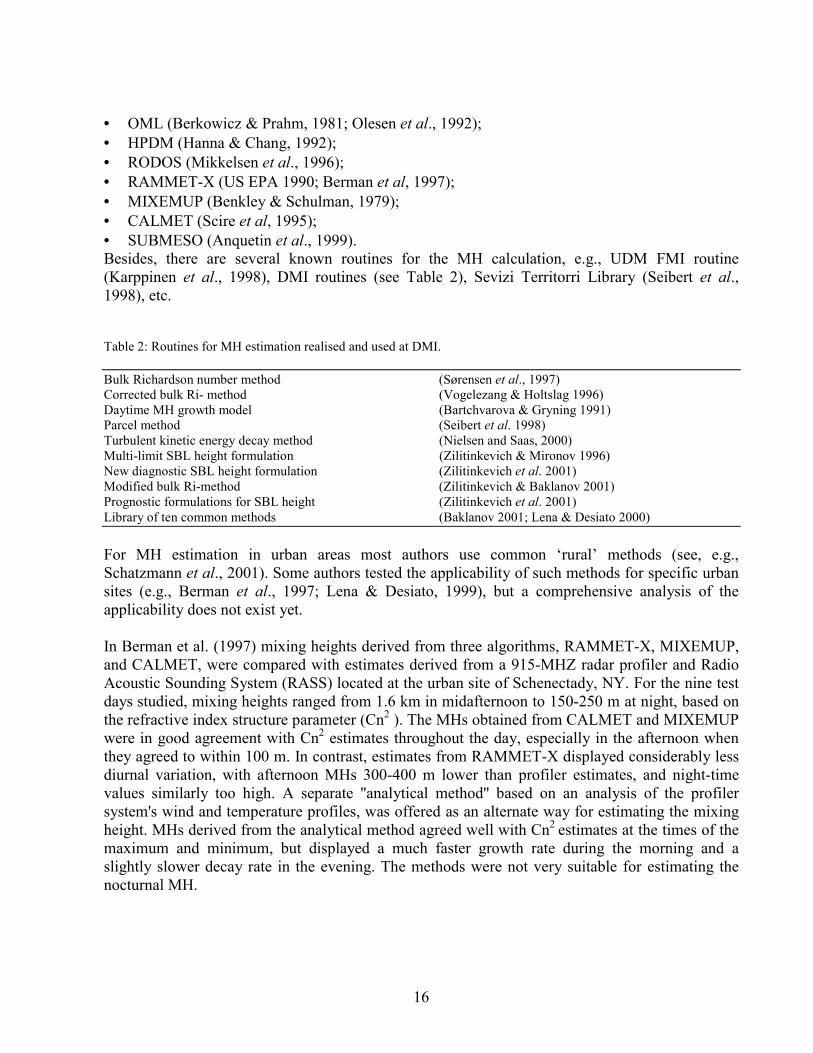
Table 2: Routines for MH estimation realised and used at DMI.

Bulk Richardson number method (Sørensen et al., 1997)Corrected bulk Ri- method (Vogelezang & Holtslag 1996)Daytime MH growth model (Bartchvarova & Gryning 1991)Parcel method (Seibert et al. 1998)Turbulent kinetic energy decay method (Nielsen and Saas, 2000)Multi-limit SBL height formulation (Zilitinkevich & Mironov 1996)New diagnostic SBL height formulation (Zilitinkevich et al. 2001)Modified bulk Ri-method (Zilitinkevich & Baklanov 2001)Prognostic formulations for SBL height (Zilitinkevich et al. 2001)Library of ten common methods (Baklanov 2001; Lena & Desiato 2000)

For MH estimation in urban areas most authors use common ‘rural’ methods (see, e.g.,Schatzmann et al., 2001). Some authors tested the applicability of such methods for specific urbansites (e.g., Berman et al., 1997; Lena & Desiato, 1999), but a comprehensive analysis of theapplicability does not exist yet.

In Berman et al. (1997) mixing heights derived from three algorithms, RAMMET-X, MIXEMUP,and CALMET, were compared with estimates derived from a 915-MHZ radar profiler and RadioAcoustic Sounding System (RASS) located at the urban site of Schenectady, NY. For the nine testdays studied, mixing heights ranged from 1.6 km in midafternoon to 150-250 m at night, based onthe refractive index structure parameter (Cn2 ). The MHs obtained from CALMET and MIXEMUPwere in good agreement with Cn2 estimates throughout the day, especially in the afternoon whenthey agreed to within 100 m. In contrast, estimates from RAMMET-X displayed considerably lessdiurnal variation, with afternoon MHs 300-400 m lower than profiler estimates, and night-timevalues similarly too high. A separate ''analytical method'' based on an analysis of the profilersystem's wind and temperature profiles, was offered as an alternate way for estimating the mixingheight. MHs derived from the analytical method agreed well with Cn2 estimates at the times of themaximum and minimum, but displayed a much faster growth rate during the morning and aslightly slower decay rate in the evening. The methods were not very suitable for estimating thenocturnal MH.

17

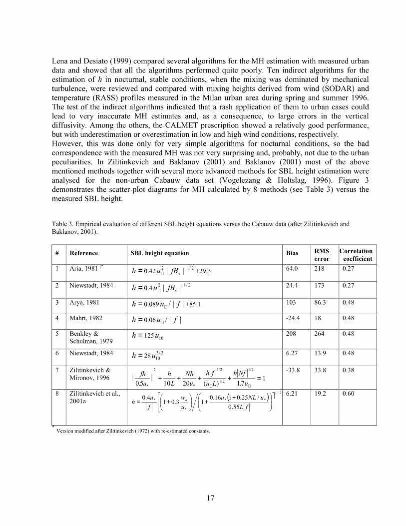
Lena and Desiato (1999) compared several algorithms for the MH estimation with measured urbandata and showed that all the algorithms performed quite poorly. Ten indirect algorithms for theestimation of h in nocturnal, stable conditions, when the mixing was dominated by mechanicalturbulence, were reviewed and compared with mixing heights derived from wind (SODAR) andtemperature (RASS) profiles measured in the Milan urban area during spring and summer 1996.The test of the indirect algorithms indicated that a rash application of them to urban cases couldlead to very inaccurate MH estimates and, as a consequence, to large errors in the verticaldiffusivity. Among the others, the CALMET prescription showed a relatively good performance,but with underestimation or overestimation in low and high wind conditions, respectively. However, this was done only for very simple algorithms for nocturnal conditions, so the badcorrespondence with the measured MH was not very surprising and, probably, not due to the urbanpeculiarities. In Zilitinkevich and Baklanov (2001) and Baklanov (2001) most of the abovementioned methods together with several more advanced methods for SBL height estimation wereanalysed for the non-urban Cabauw data set (Vogelezang & Holtslag, 1996). Figure 3demonstrates the scatter-plot diagrams for MH calculated by 8 methods (see Table 3) versus themeasured SBL height.

Table 3. Empirical evaluation of different SBL height equations versus the Cabauw data (after Zilitinkevich andBaklanov, 2001).

# Reference SBL height equation Bias RMSerror

Correlationcoefficient

1 Aria, 1981 (* =h 0.42 2/12 || −∗ sfBu +29.3 64.0 218 0.27

2 Niewstadt, 1984 =h 0.4 2/12 || −∗ sfBu 24.4 173 0.27

3 Arya, 1981 =h 0.089 ||/ fu∗ +85.1 103 86.3 0.48

4 Mahrt, 1982 =h 0.06 ||/ fu∗ -24.4 18 0.48

5 Benkley &Schulman, 1979

=h 125 10u 208 264 0.48

6 Niewstadt, 1984 =h 28 2/310u 6.27 13.9 0.48

7 Zilitinkevich &Mironov, 1996 fh

uhL

Nhu

h fu L

h Nfu0 5 10 20 17

12 1 2

1 2

1 2

. ( ) .* *

/

/

/

� � + + + + =∗ ∗

-33.8 33.8 0.38

8 Zilitinkevich et al.,2001a ( )

2/1

**

*

*

55.0/25.0116.0

13.014.0 �

���

�

��

�

�

��

++��

�

���

+=

fLuNLu

uw

fu

h h6.21 19.2 0.60

* Version modified after Zilitinkevich (1972) with re-estimated constants.

18

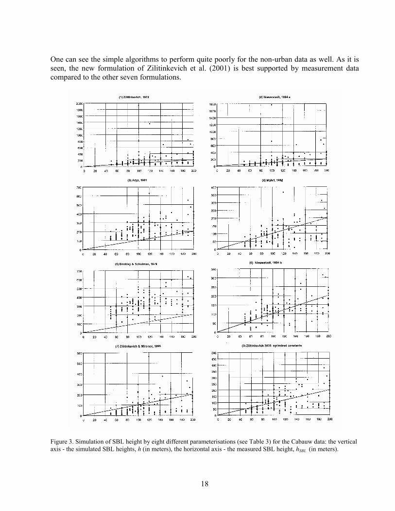
One can see the simple algorithms to perform quite poorly for the non-urban data as well. As it isseen, the new formulation of Zilitinkevich et al. (2001) is best supported by measurement datacompared to the other seven formulations.

Figure 3. Simulation of SBL height by eight different parameterisations (see Table 3) for the Cabauw data: the verticalaxis - the simulated SBL heights, h (in meters), the horizontal axis - the measured SBL height, hSBL (in meters).

19

Another interesting method to be tested for urban conditions was suggested by Joffre et al. (2001).They investigated the variability of the stable and unstable boundary layer height applyingdifferent characteristic length scales and combinations of them (JKHK method). They found that,under stable conditions, a great deal of the variability of the mixing height is explained with thescales LN = u*/N and L. For unstable conditions with buoyant and mechanical turbulenceproduction, the MH is best determined with an expression based on a dimensionless form of theturbulence kinetic energy equation (Kitaigorodskii & Joffre, 1988) with the mixing height scaledby L and depending on the stability parameter µN = LN/L and on N/f.

Another method, commonly proposed in scientific publications for the MH estimation, is based onthe Richardson number approach. It differs in formulation, choice of the levels over which thegradients are determined and in value of the critical Richardson number, Ric, and it canunderestimate the SBL height (Seibert et al., 1998; Baklanov, 2001). Following Zilitinkevich &Baklanov (2001), we can distinguish four different Ri methods. 1. Gradient Richardson number. Infinitesimal disturbances in a steady-state homogeneous stablystratified sheared flow decay if the gradient Richardson number Ri exceeds a critical value Ric,

( )

( ) ( ) 25.0Ri//

/Ri 22 =>∂∂+∂∂

∂∂≡ cv

zvzuzθβ .

(1)

Accordingly, the turbulent boundary layer height, Eh , is deduced from inequalities cRiRi < at z <

Eh and cRiRi > at z > Eh . 2. Bulk Richardson number. An alternative, widely used method of estimating h employs, insteadof the gradient Richardson number Ri, the boundary-layer bulk Richardson number, BRi , specifiedas

2RiU

hvB

θβ∆≡ => v

BcE

Uhθβ∆

=2Ri (2)

through the wind velocity at the upper boundary of the layer, )()( 22 hvhuU += , and the virtualpotential temperature increment across the layer, )0()( vvv h θθθ −=∆ . 3. Finite-difference Richardson number. The idea is to exclude the lower portion of the SBL and todetermine a “finite-difference Richardson number”, FRi , on the basis of increments

vδθ = )()( 1zh vv θθ − and Uδ =hz

zzzvzu

=

=+

2

)()( 22 over the height intervals hzz <<1 and

hzz <<2 . Assuming the existence of its standard critical value, FcRi , the equilibrium SBL heightformulation becomes

20

v

Fc

E

EE

Uzh

zhhβδθδ 2

1

22 )(Ri)( =

−−≈ .

(3)

4. Modified Richardson number method. Analysis of different estimations of Ribc for calculation ofh shows a broad variation of Ribc values from 0.11 to 3.0 (see Table 2 in Zilitinkevich & Baklanov,2001). They showed that the SBL critical bulk Richardson number, RiBc, is not a constant andevidently increases with increasing free flow stability and very probably depends on the surfaceroughness length, the Coriolis parameter and the geostrophic wind shear in baroclinic flows. TheRichardson-number-based calculation techniques can be recommended only for rough estimates ofthe SBL height. For practical use Zilitinkevich and Baklanov (2001) recommended:

||

0024.01371.0RifN

Bc +≈ . (4)

For more accurate SBL height calculations within 1-D and 3-D models, respectively, thediagnostic and prognostic formulations (Zilitinkevich et al., 2001) are recommended. It isnecessary to mention that diagnostic methods for estimation of the urban MH are not good enoughdue to the strong horizontal inhomogeneity and temporal non-stationarity of the UBL and non-local character of urban MH formation. So, it is suggested within 3-D models to calculate the SBLheight, h, more accurately on the basis of the prognostic formulation and accounting for thehorizontal transport through the advection term and the sub-grid scale horizontal motions throughthe horizontal diffusivity hK (Zilitinkevich & Baklanov, 2001):

hKhhfChth

hCQEE2)(|| ∇+−−=∇⋅+

∂∂ V , (5)

where V ),( vu= is the horizontal velocity vector, CE is a constant (CE ≈ 1), CQEh is the equilibriumMH, calculated from a diagnostic formulation (e.g., Zilitinkevich et al., 2001).

5. Specific methods for the urban or other IBL height estimationJust a few authors suggested specific methods for MH determination in urban areas. As it wasmentioned above they can be distinguished in two categories: (i) with correction of heat fluxes, and(ii) with estimation of IBL height growth. The first category is not very interesting for the analysisbecause it uses the above-discussed methods with corrected values of the urban heat flux androughness. Let’s consider the second category.

It should be considered in the bounds of general methods to estimate the growing height of theinternal boundary layers with sudden changes of the surface roughness (smooth-to-rough or rough-to-smooth). Such approaches of the IBL or the blending height were actively developed forestimation of the IBL in coastal areas (see e.g., Panovsky & Dutton, 1984; Walmsley, 1989;Garratt, 1990; Wringht et al., 1999). Such an approach can be used for the estimation of the heightof the internal urban boundary layer, so-called downwind ‘urban plume’ and the rural IBL (seeFigure 1).

21

E.g., Henderson-Sellers (1980) developed a simple model for the urban MH as a function ofdistance downwind into the city. Nkemdirim (1986) tested and further improved the Summers(1964) formulation for the UMH:

2/1

0

2 �

���

�=

ucHxhp

k

αρα , (6)

where H is the cumulative heat flux between x0 and xk; xk is the downwind distance. Theformulation was verified for cities of New York and Calgary. It was shown that it could be usedfor a rough UMH estimation, but only for wind velocities u < 4 m/s.

Melas and Kambezidis (1992) studied the height of the thermal internal boundary layer over anurban area under sea-breeze conditions and compared it with the data of the ATHens InternalBoundary Layer Experiment (ATHIBLEX) in summer 1989 and 1990. For the IBL heightestimation they analysed three slab methods: (i) - Gamo et al. (1983), (ii) – Venkatram (1986), (iii)- Gryning and Batchvarova (1990); one simple empirical diagnostic method as a function of thedistance to city in wind direction, and one similarity model (Miyake, 1965). It was found that thesimilarity model of Miyake (1965) failed to give any reasonable prediction, indicating that modelsshould not be extended beyond their stability and fetch range. Relations based on the slab modelsshowed a high correlation with observations, but the observed thermal IBL heights wereunpredicted unless both convective and mechanical turbulence were taken into account. Theformulation proposed by Gryning and Batchvarova (1990) was found to be in good agreement withthe measurements. In the bounds of the local equilibrium concept the thermal IBL height wassuggested to grow as xp where p depends upon several parameters of the IBL.

In Gryning and Batchvarova (1996) the above mentioned slab model on a zero-order scheme wasextended for the internal boundary layer over terrain with abrupt changes of surface for nearneutral and unstable atmospheric conditions. The equation for the height h of the internalboundary layer (Gryning and Batchvarova, 1996) is:

( ) ( )[ ]( )γθ

∂∂

∂∂

∂∂

κγκs

sww

yhv

xhu

th

LBhAgTCu

LBhAh ''2

1221

2=

����

�−++

�

���

��

�

−++

−+∗ , (7)

where u and v are the horizontal components of the mean wind speed in the internal boundarylayer in the x and y directions, t is time, *u is the friction velocity, ( )′ ′w sθ - the kinematic heat

flux, γ - the potential temperature gradient, sw - the mean vertical air motion above the boundarylayer, L the Monin-Obukhov scaling length, κ is the von Karman constant, and A, B and Cempirical dimensionless constants. The model includes coastline curvature and spatially varyingwinds and was solved numerically for the height of the internal boundary layer. In the following

22

papers (Batchvarova & Gryning, 1998; Batchvarova et al., 1999; Gryning & Batchvarova, 2001)the authors applied this model for urban areas with a coastline and showed its good applicability.E.g., Batchvarova et al. (1999) tested the ability of two quite different models to simulate thecombined spatial and temporal variability of the internal boundary layer in an area of complexterrain and coastline during one day. The simple applied slab model of Gryning and Batchvarova(1996), and the Colorado State University Regional Atmospheric Modelling System (CSU-RAMS)were tested by comparison with data gathered during a field study (called Pacific '93) ofphotochemical pollution in the Lower Fraser Valley of British Columbia, Canada. The data utilisedthere were drawn from tethered balloon flights, free flying balloon ascents, and downlooking lidaroperated from an aircraft flown at roughly 3500 m above sea level. Both models were found torepresent the temporal and spatial development of the internal boundary-layer height over theLower Fraser Valley very well, and reproduced many of the finer details revealed by themeasurements.

Cleugh and Grimmond (2001) also assessed the validity of the simple slab model of the CBL - thiswas integrated forward in time using local-scale measured heat and water vapour fluxes, to predictthe MH, temperature and humidity - for the Sacramento urban region, California. The prediction ofthe height of well-mixed CBLs using the slab model agreed fairly closely to the measured values.Of the four different CBL growth schemes used, the Tennekes and Driedonks (1981) model wasfound to give the best performance.

Proceeding from the above overview of different methods of the MH estimation for urban areas,we can conclude that for the convective and neutral daytime UBL the simple slab models (e.g.Gryning and Batchvarova, 2001) perform quite well. However, for the nocturnal UBL with stableand complex stratification most of the common methods perform not well enough. The urban SBLapparently needs a new theory for a better understanding of the SBL processes. One of suchmodern attempts is the parameterisation of Zilitinkevich et al. (2001), based on the newlydeveloped non-local turbulence transport theory. Such methods need further adjustments for urbanconditions and verifications versus urban data.

6. Concluding remarks The urban boundary layer, in comparison with ‘rural’ homogeneous PBLs, is characterised bygreatly enhanced mixing, resulting from both the large surface roughness and increased surfaceheating, and by horizontal inhomogeneity of the MH and other meteorological fields due tovariations in surface roughness and heating from rural to central city areas. So, it is reasonable toconsider the UBL as a specific case of the PBL over a non-homogeneous terrain. This related, firstof all, to abrupt changes of the surface roughness and the urban surface heat fluxes. Specificmethods for MH determination in urban areas can be distinguished in two categories: (i) with alocal correction of the heat fluxes due to urban effects, and (ii) with estimations of the internalboundary layer (IBL) height growth. General suggestions concerning the applicability of ‘rural’ methods of the MH estimation forurban areas:

23

• For estimation of the daytime MH, applicability of common methods is more acceptable thanfor the nocturnal MH.• For the convective UBL the simple slab models (e.g. Gryning and Batchvarova, 2001) werefound to perform quite well.• The formation of the nocturnal UBL occurs in a counteraction with the negative ‘non-urban’surface heat fluxes and positive anthropogenic/urban heat fluxes, so the applicability of thecommon methods for the SBL estimation is less promising.• The determination of the SBL height needs further developments and verifications versusurban data. As a variant of the methodics for SBL MH estimation the new Zilitinkevich et al.(2001) parameterisation can be suggested in combination with a prognostic equation for thehorizontal advection and diffusion terms (Zilitinkevich and Baklanov, 2001).• Meso-meteorological and NWP models with modern high-order non-local turbulence closuresgive promising results (especially for the CBL), however currently the urban effects in suchmodels are not included or included with great simplifications (Baklanov et al., 2001). Therefore, it is very important to test different MH schemes not specifically designed for the urbanenvironment against urban MH or IBL schemes for different data sets (for nocturnal conditionsfirst of all) from different urban sites to gain insight in the possible improvements. It would also beof use to know which of the parameterisations are most sensitive to changes of whichenvironmental variables.

ReferenceAnquetin, S., Chollet, J. P., Coppalle, A., Mestayer, P., and Sini, J. F. (1999). The Urban Atmosphere Model

SUBMESO, Proc. EUROTRAC Symp. ‘98, P.M. Borrel & P. Borrel eds., WIT Press.Arya, S. P. S., (1981). Parameterizing the height of the stable atmospheric boundary layer, J. Appl.

Meteorol. 20, 1192-1202.Arya, S. P. S. and Byun, D. W., (1987) Rate equations for the planetary boundary-layer depth (urban vs

rural). IN: Modeling the urban boundary-layer. American Meteorological Society, Boston, pp. 215-251.Baklanov, A., (2000a) Application of CFD methods for modelling in air pollution problems: possibilities

and gaps, Environmental Monitoring and Assessment, 65: 181-190.Baklanov, A. (2000b) Possible improvements in the DMI-HIRLAM for parameterisations of long-lived

stably stratified boundary layer. DMI Internal Report, No. 00-15, 15 p.Baklanov, A., (2001a). NWP modelling for urban air pollution forecasting: possibilities and shortcomings.

DMI Technical Report, No. 01-12, 19 pBaklanov, A. (2001b) Parameterisation of SBL height in atmospheric pollution models. NATO/CCMS

International Technical Meeting on Air Pollution Modelling and its Application. ITM-2001, 15-19October 2001, Louvain-la-Neuve, Belgium, pp. 303-310.

Baklanov, A., A. Rasmussen, B. Fay, E. Berge and S. Finardi, (2001). Potential and Shortcomings of NWPModels in Providing Meteorological Data for UAP Forecasting. Ext. abstract to the Third Urban AirQuality Conference, Loutraki, Greece. CD-ROM, paper PL.4.1.

Batchvarova, E. and Gryning, S.-E., (1991). Applied model for the growth of the daytime mixed layer.Boundary-Layer Meteorology, 56(3): 261-274.

Batchvarova, E. and Gryning, S.-E., (1998). Wind Climatology, Atmospheric Turbulence and InternalBoundary-Layer Development in Athens During the MEDCAPHOT-Trace Experiment, Atmos. Environ.32, 2055-2069.

24

Batchvarova, E., Cai, X., Gryning, S.-E., Steyn, D., (1999). Modelling internal boundary-layer developmentin a region with a complex coastline. Boundary-Layer Meteorology, 90: 1-20.

Benkley, C.W. and Schulman, L.L., (1979). Estimating mixing depths from historical meteorological data,Journal of Applied Meteorology, 18, 772-780.

Berkowicz, R. and Prahm, L.P. (1982). Sensible heat flux estimated from routine meteorological data by theresistance methode. J. Appl. Meteorol., 21, 1845-1864.

Berman, S., Ku, J.-Y., Zhang, J. & Rao, S. T. (1997). Uncertainties in estimating the mixing depth:comparing three mixing-depth models with profiler measurements. Atmospheric Environment, 31(18):3023-3039

Bornstein, R. D. (2001). Currently used parameterisations in numerical models. Workshop on UrbanBoundary Layer Parameterisations. COST 715, Zürich, May 24-25 2001.

Byun, D. W. & Arya, S. P. S. (1990). A two-dimensional mesoscale numerical model of an urban mixedlayer. I: Model formulation, surface energy budget, and mixed layer dynamics. AtmosphericEnvironment, 24(4): 829-844.

Chen, W., H. Kuze, A. Uchiyama, Y. Suzuki and N. Takeuchi, (2001). One-year observation of urbanmixwed layer characteristics at Tsukuba, Tokio using a micro pulse lidar. Atmospheric Environment,35: 4273-4280.

Cleugh, H. A. and Grimmond, C. S. B. (2001) Modelling regional scale surface energy exchanges and CBLgrowth in heterogeneous, urban-rural landscape. Boundary-Layer Meteorology, 98: 1-31.

Cooper, D. I., Eichinger, W. E. (1994). Structure of the atmosphere in an urban planetary boundary layerfrom lidar and radiosonde observations. Journal of Geophysical Research, 99(D11): 22937-22948

Cuxart, J., Bougeault, P., and Redelsperger, J.-L. (2000). A turbulence scheme allowing for mesoscale andlarge eddy simulations, Q. J. R. Meteorol. Soc. 126: 1-30.

Donev, E., Panchev, St., Kolev, I. & Zeller, K. (1993). The morning boundary layer transition in responseto the surface heat flux at an urban site in Sofia. Bulgarian Journal of Meteorology and Hydrology, 4(4):186-195

Donev, E., Zeller, K., Panchev, St. & Kolev, I. (1995). Boundary layer growth and lapse rate changesdetermined by lidar and surface heat flux in Sofia. Acta Meteorologica Sinica, Beijing, China, 9(1): 101-111

Dupont, E., Menut, L., Carissimo, B., Pelon, J., Flamant, P. (1999). Comparison between the atmosphericboundary layer in Paris and its rural suburbs during the ECLAP experiment. Atmospheric Environment,33(6): 979-994

Evers, K., Niesser, J. & Weiss, E. (1987). Acoustic sounding of the urban boundary layer over Berlin-Adlershof in summer. Zeitschrift für Meteorologie, 37(5): 241-252 (German)

Fisher B., Erbrink J., Finardi S., Jeannet Ph., Joffre S., Morselli M., Pechinger U., Seibert P. & D.Thomson, (1998). Harmonization of the Preprocessing of meteorological data for atmosphericdispersion models. COST 710 Final Report, CEC Publication EUR 18195, Luxembourg, 431 pp.

Gamo, M., S. Yamamoto, O. Yokoyama and H. Yoshikado (1983). Structure of the free convective internalboundary layer during the sea breeze. J. Meteor. Soc. of Japan, 61, 110-124.

Garratt, J. R., (1990). The Internal Boundary Layer - A Review, Boundary-Layer Meteorol. 50, 171-203.Godowitch, J. M. (1986). Characteristics of vertical turbulent velocities in the urban convective boundary

layer. Boundary-Layer Meteorology, 35(4): 387-407Godowitch, J. M., Ching, J. K. S., Clark, J. F. (1985). Evolution of the nocturnal inversion layer at an urban

and nonurban location. Journal of Climate and Applied Meteorology, 24(8): 791-804.Godowitch, J. M., Ching, J. K. S., Clarke, J. F. (1987). Spatial variation of the evolution and structure of

the urban boundary layer. Boundary-Layer Meteorology, 38(3): 249-272.Gryning, S.-E. and E. Batchvarova (1990). Analytical model for the growth of the coastal internal boundary

layer during onshore flow. Quarterly Journal of the Royal Meteorological Society, 116(491): 187-203.

25

Gryning, S.-E. and E. Batchvarova (1996). A model for the height of the internal boundary layer over anarea with an irregular coastline. Boundary-Layer Meteorology, 78: 405-413.

Gryning, S.-E. and E. Batchvarova (2001). Mixing height in urban areas: will ‘rural’ parameterisationswork? COST-Action 715 Workshop on Urban Boundary Layer Parameterisations. Zürich, May 24-252001, 10 p.

Hanna, S. R. & J. C. Chang, (1992). Boundary-layer parameterizations for applied dispersion modelingover urban areas. Boundary-Layer Meteorology, 58(3): 229-259

Henderson-Sellers, A. (1980). A simple numerical simulation of urban mixing depths. Journal of AppliedMeteorology, 19: 215-218

Hildebrand, P.H. & Ackerman, B. (1984). Urban effects on the convective boundary layer. Journal of theAtmospheric Sciences, 41(1): 76-91

Joffre, S. M., M. Kangas, M. Heikinheimo, S. A. Kitaigorodskii, (2001). Variability of the stable andunstable atmospheric boundary layer height and its scales over a boreal forest. Boundary LayerMeteorol., 99(3), 429-450.

Kambezidis, H. D., Peppes, A. A., Melas, D. (1995). An environmental experiment over Athens urban areaunder sea breeze conditions. Atmospheric Research, 36(1-2): 139-156

Karppinen, A., J. Kukkonen, G. Nordlund, E. Rantakrans, and I. Valkama, (1998). A dispersion modellingsystem for urban air pollution. Finnish Meteorological Institute, Publications on Air Quality 28.Helsinki, 58 p.

Karppinen, A., S.M. Joffre and P. Vaajama (1997): Boundary-layer parameterisation for Finnish regulatorydespersion models. Int. J. Environment and Pollution, 8, 3-6, 557-564.

Kerschgens, M. J. & Suer, H. (1988). Energetic feedback between urban climate and diffusion ofatmospheric pollutants. IN: International Symposium on Environmental Meteorology, 1st, Würzburg,W. Germany, Sept. 29-Oct. 1, 1987, Proceedings, Dordrecht, Holland, Kluwer Academic Publishers,1988, p. 335-344.

Kitaigorodskii, S. A. and S. M. Joffre, (1988). In search of a simple scaling for the height of the stratifiedatmospheric boundary layer. Tellus 40A(5), 419 - 433.

Kolev, I., P. Savov, B. Kaprielov, O. Parvanov and V. Simeonov, (2000). Lidar observation of thenocturnal boundary layer formation over Sofia, Bulgaria. Atmospheric Environment, 34(19): 3223-3235.

Kumari, M. (1985). Diurnal variation of mean mixing depths in different months at Delhi. Mausam, NewDelhi, 36(1): 71-74

Kurbatskii, A.F. (2001) Computational modelling of the turbulent penetrative convection above the urbanheat island in a stably stratified environment. J. Appl. Meteor., 40: 1848-1761.

Lena, F. and Desiato, F. (1999) Intercomparison of nocturnal mixing height estimate methods for urban airpollution modelling. Atmospheric Environment, 33(15): 2385-2393.

Liu, X. & Ohtaki, E. (1997) An independent method to determine the height of the mixed layer. Boundary-Layer Meteorology, 85(3): 497-504.

Lokoshchenko, M. A., Isaev, A. A., Kallistratova, M. A. & Pekur, M. S. (1993). Studies of the atmosphericboundary layer over Moscow by remote sensing and in situ methods. Russian Meteorology andHydrology, New York, NY, 9: 13-24

Marsik, F. J., Fischer, K. W., McDonald, Tracey D., Samson, Perry J. (1995) Comparison of methods forestimating mixing height used during the 1992 Atlanta Field Intensive. Journal of Applied Meteorology,34(8): 1802-1814.

Melas, D., Kambezidis, H. D. (1992). The depth of the internal boundary layer over an urban area undersea-breeze conditions. Boundary-Layer Meteorology, 61(3): 247-264

Miao, M. (1987). Numerical modeling of the nocturnal PBL over the urban heat island in Changzhou city.Boundary-Layer Meteorology, 41(1/4): 41-56

26

Mikkelsen, T., S. Thykier-Nielsen, P. Astrup, J. M. Santabárbara, J.H. Sørensen, A. Rasmussen, L.Robertson, A. Ullerstig, S. Deme, R. Martens, J. G. Bartzis and J. Päsler-Sauer (1997). MET-RODOS: AComprehensive Atmospheric Dispersion Module. Radiat. Prot. Dosim. 73, 45–56.

Miyake, M., (1965). Transformation of the ABL over inhomogeneous surfaces. Sci. Report Contract (NR307-252) 477(24).

Nielsen, N-W. and B.H. Saas, (2000). A lower boundary condition for the mixing length in the CBRturbulence scheme. HIRLAM Newsletter, 35, 128-136.

Nieuwstadt , F.T.M., (1984). Some aspects of the turbulent stable boundary layer, Boundary-LayerMeteorology, 30, 31-55.

Nieuwstadt, F.T.M., (1984). The turbulent structure of the stable, nocturnal boundary layer, J. Atmos. Sci.41, 2202-2216.

Nkemdirim, L.C. (1986). Mixing depths and wind speed in an urban airshed: a note on the limits to arelationship. Atmospheric Environment, 20(9): 1829-1830

Olesen, H. R., Løfstrøm, P., Berkowicz, R. and Jensen, A. B., (1992). An improved dispersion model forregulatory use: the OML model. In: van Dop, Han and Kallos, George (eds.), Air pollution modeling andits application IX. New York, NY, Plenum Press, 1992. p. 29-38.

Panovsky, H.A. & J.A. Dutton, (1984). Atmospheric turbulentce. Wiley, NY, 397 pp.Penenko, V.V. and A.E. Aloyan, (1974). Numerical method for some meso-meteorological problems with

free top of atmospheric mass. Trudy ZapSibNII, Novosibirsk, 14, 52-66. (in Russian)Penenko, V.V. and A.E. Aloyan, (1985). Models and Methods for Environmental Problems. Nauka:,

Novosibirsk, 256 p. (pp. 49-55) (in Russian)Piringer, M. (1988). Determination of mixing heights by sodar in an urban environment. IN: International

Symposium on Environmental Meteorology, 1st, Würzburg, W. Germany, Sept. 29-Oct. 1, 1987,Proceedings, Dordrecht, Holland, Kluwer Academic Publishers, 1988, p. 425-444.

Piringer, M., A. Baklanov, K. De Ridder, J. Ferreira, S. Joffre, A. Karppinen, P. Mestayer, D. Middleton,M. Tombrou, R. Vogt, (2001). The surface energy budget and the mixing height in urban areas: Statusreport of Working Group 2 of COST-Action 715. Ext. abstract to the Third Urban Air QualityConference, Loutraki, Greece. CD-ROM, paper Pl 1.3.

Piringer, M. and K. Baumann (1999): Modification of a valley wind system by an urban area - experimentalresults. Meteorol. Atmos. Phys. 71, 117 - 125.

Piringer, M., Baumann, K. & Langer, M. (1998). Summertime heights at Vienna, Austria, estimated fromvertical soundings and by a numerical model. Boundary-Layer Meteorology, 89: 25-45.

Piringer, M., Editor (2000) Surface energy balance in urban areas. Extended abstracts of an ExpertMeeting. WG-2 COST Action 715, Antwerp, Belgium, 12 April 2000 (submitted to EC-COST).

Railo, M., Editor (1997). Urban Episodes. Problems and Action Plans: Paris, Berlin, Helsinki, Turku.IImansuojelu. Special Issue. 6, 29 pp.

Rasmussen, A., J.H. Sørensen and N.W. Nielsen. (1997). Validation of Mixing Height Determined fromVertical Profiles of Wind and Temperature from the DMI-HIRLAM NWP Model in Comparison withRadiosoundings. In: The Determination of the Mixing Height - Current Progress and Problems.EURASAP Workshop Proceedings, 1-3 October, 1997, Risø National Laboratory, Eds: S.-E. Gryning, F.Beyrich and E. Batchvarova, pp. 101-104

Rasmussen, A., J. H. Sørensen, N. W. Nielsen. and B. Amstrup (1999): Uncertainty of MeteorologicalParameters from DMI-HIRLAM. Report RODOS (WG2)TN(99)12.

Rayner, K. N. & Watson, I. D. (1991). Operational prediction of daytime mixed layer heights for dispersionmodelling. Atmospheric Environment, 25A(8): 1427-1436.

Roth, M. (2000) Review of atmospheric turbulence over cities. Quart. J. Roy. Meteor. Soc, 126(564): 941-990.

27

Rotach, M.W., V. Mitev and R. Vogt (2001) BUBBLE - current status of the experiment and plannedinvestigations/evaluations of the mixing height. COST715 Workshop ’Mixing heights and inversions inurban areas’, Meteo-France, Toulouse, 3-5.10.2001.

Sass, B. H., Nielsen, N. W., Jørgensen, J.U., Amstrup, B., and Kmit, M., (2000). The operational HIRLAMsystem, DMI Technical report 00-26. http://www.dmi.dk/f+u/publikation/tekrap/2000/Tr00-26.pdf.

Said, F., B. Campistron, A. Coppalle, A. Dabas, Ph. Drobinsky, E. Fréjafon, E. Gizard, A. Mériaux and P.Mestayer (2001) Influence of sea breeze and relief on the mixing height during ESCOMPTE in theMarseille area. COST715 Workshop ’Mixing heights and inversions in urban areas’, Meteo-France,Toulouse, 3-5.10.2001.

Sang, J. & Liu, W. (1990). An analysis on flow and temperature structure of wintertime urban boundarylayer. Acta Meteorologica Sinica, Beijing, China, 48(4): 459-468

Schatzman, M., J. Brechler and B. Fisher, Editors, (2001). Preparation of meteorological input data forurban site studies. Proceedings of the workshop, 15 June 2000, Prague, Czech Republic. EC, CostAction 715, EUR 19446, 101 pp.

Scire, J.S., E.M. Insley, R.J. Yamartino and M.E. Fernau, (1995). A user’s guide for the CALMETmeteorological model, EARTH TACH, 1995.

Seaman, N.L. (1989). Numerical studies of urban planetary boundary-layer structure under realisticsynoptic conditions. Journal of Applied Meteorology, 28(8): 760-781

Seibert, P., Beyrich, F., Gryning, S.-E., Joffre, S., Rassmussen, A. and Tercier, Ph., (1998). Mixing HeightDetermination for Dispersion Modelling. Report of Working group 2. COST Action 710. In: Fisher et al(Eds.), Preprocessing of Meteorological data for Dispersion Modelling. May 1997.

Soudine, A. (2001) Personal communications. October 2001. WMO.Summers, P. W. (1965). An urban heat island model: its role in air pollution problems with applications to

Montreal. First Canadian Conf. on Micrometeorology. Toronto, CMOS, 22 pp.Summers, P. W. (1977). Application of the urban mixing-depth concept to air pollution problems. IN:

United States Forest Service, Northeastern Experiment Station, Upper Darby, PA., General TechnicalReport NE-25, 1977, p. 273-277.

Sørensen, J.H., A. Rasmussen and H. Svensmark, (1996). Forecast of Atmospheric Boundary-Layer Heightfor ETEX Real-time Dispersion Modelling, Phys. Chem. Earth, Vol 21, No. 5-6, pp. 435-439.

Tennekes, H. and A. G. M. Driedonks, (1981). Basic entrainment equations for the atmospheric boundarylayer. Boundary-Layer Meteorology, 20(4): 515-531

US EPA, (1990). User’s guide for the Urban Airshed Model. Vol.2: User’s manual for the UAM modelingsystem, EPA-450/4-90-007B.

Venkatram, A. (1986). An examination of methods to estimate the height of the coastal internal boundarylayer. Boundary-Layer Meteorology, 36: 149-156.

Vogelezang, D.H.P. and Holtslag, A.A.M., (1996). Evolution and model impacts of the alternativeboundary layer formulations. Boundary-Layer Meteor., 81, 245-269.

Walmsley, J.L. (1989). Internal boundary-layer height formulae – a comparison with atmospheric data.Boundary-Layer Meteor., 47, 251-262.

Westcott, N. (1989). Influence of mesoscale winds on the turbulent structure of the urban boundary layerover St. Louis. Boundary-Layer Meteorology, 48(3): 283-292

Wringht, S.D., Elliot, L., Ingham, D.B. & Hewson, M.J.C. (1999). The adaptation of the atmosphericboundary layer to a change in surface roughness. Boundary-Layer Meteorology,

Zhang, A., Sun, C. & Yi, T. (1991). Observing results of the atmospheric mixed layer in Beijing area andthe evaluation of theoretical models. Acta Meteorologica Sinica, Beijing, China, 5(5): 541-550

Zhang, K., Mao, H., Civerolo, K., Berman, S., Ku, Y.-Y., Rao, S. T., Doddridge, B., Philbrick, C. R., Clark,R. (2001). Numerical investigation of boundary layer evolution and nocturnal low-level jets: localversus non-local PBL schemes. Envir. Fluid Mechanics, 1: 171-208.

28

Zilitinkevich, S. & Baklanov, A. (2001). Calculation of the height of stable boundary layers in operationalmodels. Boundary Layer Meteorology (accepted), (available also as DMI Scientific Report, No. 01-07http://www.dmi.dk/f+u/publikation/vidrap/2001/Sr01-07.pdf)

Zilitinkevich, S. & Mironov, D. (1996). A multi-limit formulation for the equilibrium depth of a stablystratified boundary layer. Boundary-Layer Meteorology, 81(3-4): 325-351.

Zilitinkevich, S., A. Baklanov, J. Rost, A.-S. Smedman, V. Lykosov, P. Calanca, (2001). Diagnostic andprognostic equations for the depth of the stably stratified Ekman boundary layer. Quart. J. Roy. Meteor.Soc., 128 (579).

29

A recommendation for turbulence parameterisation in German guidelines

for the calculation of dispersion in the atmospheric boundary layer

– improvements and remaining problems –

K. Maßmeyer∗ and R. Martens∗∗ 1

∗ Fachhochschule Lippe und Höxter - University of Applied Sciences -, Abteilung Höxter, FachbereichTechnischer Umweltschutz, An der Wilhelmshöhe 44, D 37671 Höxter

∗∗ Gesellschaft für Anlagen- und Reaktorsicherheit mbH, Schwertnergasse 1, D 50667 Köln

Keywords:Dispersion modelling, turbulence parameters, standard deviations of wind speed components,Lagrangian time scales

AbstractCommon approaches for the turbulence parameterisation (standard deviations of wind speedcomponents σui and Lagrangian time scales TLi) for practical purposes within dispersionmodels are based on similarity theory with empirical formulas derived from meteorologicalfield experiments. The principal shape of these formulas is derived via the theory ofhomogeneous and stationary turbulence accounting for the inhomogeneity of the boundarylayer by empirical corrections. A great variety of such formulas exists in which the state ofthe atmosphere is characterised by the following input parameters: roughness length, Monin-Obukhov length, friction velocity and mixing layer height which have to be derived via ameteorological pre-processor. These formulas give different results for the same atmosphericstability, discontinuities and jumps at the transition between different stability regimes of theatmosphere.

Based on a review of parameterisations a working group of the German Association ofEngineers (VDI) recommended formulas which might be used for practical purposes. Thecriterion of choice are consistency with similarity theory, a consistent formulation for alltypes of dispersion models and a smooth transition between different turbulence regimes.

The formulas will be incorporated in the appendix of the amended version of the GermanTechnische Anleitung zur Reinhaltung der Luft (TA-Luft, Technical Instruction on Air QualityControl) which deals with atmospheric dispersion calculations (AUSTAL2000). Results ofdifferent dispersion experiments have been used as a validation data base.

1 Further members of the working group:

D. Etling, Institut für Meteorologie und Klimatologie, Universität HannoverM.J. Kerschgens, Institut für Geophysik und Meteorologie, Universität zu KölnW. Mix, Institut für Physik, Humboldt-Universität zu BerlinK. Nester, Institut für Meteorologie und Klimaforschung, Forschungszentrum KarlsruheH. Nitsche, Deutscher Wetterdienst, OffenbachU. Pechinger, Zentralanstalt für Meteorologie und Geodynamik, WienM. Wichmann-Fiebig, Air Quality Unit-Environment DG, European Commission

30

1 IntroductionIn the Commission on Air Pollution Prevention of VDI and DIN – Standards Committee(KRdL) experts from science, industry and administration, acting on their own responsibility,establish VDI guidelines and DIN standards in the field of environmental protection. Theydescribe the state of the art in science and technology in the Federal Republic of Germany andserve as a decision–making aid in the preparatory stages of legislation and application of legalregulations and ordinances.

For a long time the Gaussian plume model served as a working horse for a lot of differenttype of applications connected to environmental protection purposes. Dispersion parametersapplied in German guidelines were derived from dispersion experiments carried out at theresearch centres of Juelich and Karlsruhe for specified emission heights (50, 100 and 160 m)and 6 stability categories (GMBl, 1986; Bundesanzeiger, 1990). The orography at both sites isnearly flat and the roughness length lies in the order of 1 m. Stability categories for routineapplications at other sites usually are defined on the basis of synoptic oberservations – i.e.cloud cover, wind speed and time of the day – and carried out by the national weather service(DWD). Such datasets are available for more than 100 sites all over Germany.

Based on the results of recent boundary layer modelling theory – which follows the ideas ofthe so-called similarity theory – these meteorological datasets can also be applied to calculate(similarity) parameters characterising the turbulent state of the atmospheric boundary layervia a meteorological pre-processor (e.g. Holtslag, 1986; Holtslag, 1987; van Ulden, 1985).Using these similarity parameters a “universal” turbulence parameterisation (i.e. standarddeviations of wind speed components σui, Lagrangian time scales TLi) depending upon surfaceroughness and height can be established and applied to all types of atmospheric dispersionmodels. The parameterisation is based on the theory of homogeneous and stationaryturbulence accounting for the inhomogeneity by empirical corrections. The state of theatmosphere within the parameterisation is characterised by boundary layer parameters:

• roughness length z0,• Monin-Obukhov length L,• friction velocity u* and• height of the mixing layer zi.

During the last years several new technical guidelines have been developed in Germany andput into operation. They describe the characteristics and the application of different types ofatmospheric flow and dispersion models (i.e. Gaussian plume and puff models, Lagrangianmodels, Eulerian models) (VDI3783/6, 1992; VDI3945/1, 1995; VDI3945/3, 2000). Commonapproaches for the parameterisation of turbulence for practical purposes within thesedispersion models are based on similarity theory with empirical formulas based onexperiments. However, turbulence parameterisations available from literature often givedifferent results for the same atmospheric stability; they exhibit discontinuities and jumps atthe transition between different stability regimes of the atmosphere (Kerschgens et al., 2000).

Based on a review of parameterisations of σui and TLi a working group of the VDI recom-mended formulas to be used for practical purposes. The criterion of choice are consistencywith similarity theory (we recommend a von Karman constant of k = 0.4 and a “universal”Kolmogorov constant of C0 = 5.7), a consistent formulation for all types of dispersion modelsand a smooth transition between different turbulence regimes. The formulas are brieflysummarised in the following Chapter 2.

31

2. Vertical profiles of mean wind speed and turbulence parametersThe parameterisations presented below were derived from a literature survey ofmeteorological field experiments (Kerschgens et al., 2000) and are strictly valid only in thesurface boundary layer – which roughly extends between surface and a normalised height ofz/zi = 0.1. Contrary to the former parameterisation via dispersion parameters therecommended parameterisation is explicitly not a result of tracer experiments but based onmeteorological field data in connection with contemporary boundary layer modelling.

2.1 Vertical wind profileOnce the boundary layer parameters are known the vertical variation of wind speed can bederived via equation (1) as a function of stability (see e.g. Businger, 1971; Buyn, 1990;Paulson, 1970):

�

�

�

≤���

� −�

��

−−+⋅

��−−�

��

−

<≤�

��

−�

��

+��

��

��

⋅

<≤��

��

��

��

−⋅+⋅

≤��

��

�⋅−⋅+

++−

++⋅−⋅

=−−

Lz

Lz

Lz

Lzu

Lz

Lz

Lz

Lz

Lz

Lzu

Lz

Lzz

zzu

LzXX

XX

XX

zzu

zu

01 for521651120875850

452

1050 for5025428

500 for5

0 for2211

112

00

00

21

0

0

020

2

00

ln,ln,

ln

,,,ln

,ln

arctanarctanlnlnln

)(

*

*

*

*

κ

κ

κ

κ

(1)

with:41

151 ���

� ⋅−=LzX ;

41

00 151 �

���

� ⋅−=LzX ; for: 0zz ≥ .

2.2 Vertical profiles of turbulence parametersWithin the framework of the VDI-guidelines different types of dispersion models areincorporated. The parameterisation of atmospheric turbulence is handled via model specificturbulence parameters as shown in Table 1:

Table 1: Type of dispersion model and associated turbulence parameters within VDI-guideline framework

Model type Model specific turbulence parametersGaussian plume model Horizontal (σy) and vertical (σz) dispersion parameters, dependent upon source

distanceGaussian puff model Horizontal (σx, σy) and vertical (σz) dispersion parameters, dependent upon

travelling time of pollutantLagrangian particle model Standard deviations of the wind velocity components (σu, σv, σw), Lagrangian

time scales (TLx, TLy, TLz), dependent on local roughnessEulerian model Diffusion coefficients (Kx, Ky, Kz), depending on local roughness

In the following subsections formulas are summarised which enable the model specificturbulence parameterisation based on identical input information, i.e. the standard deviationsof the wind speed components and the Lagrangian time scales.

32

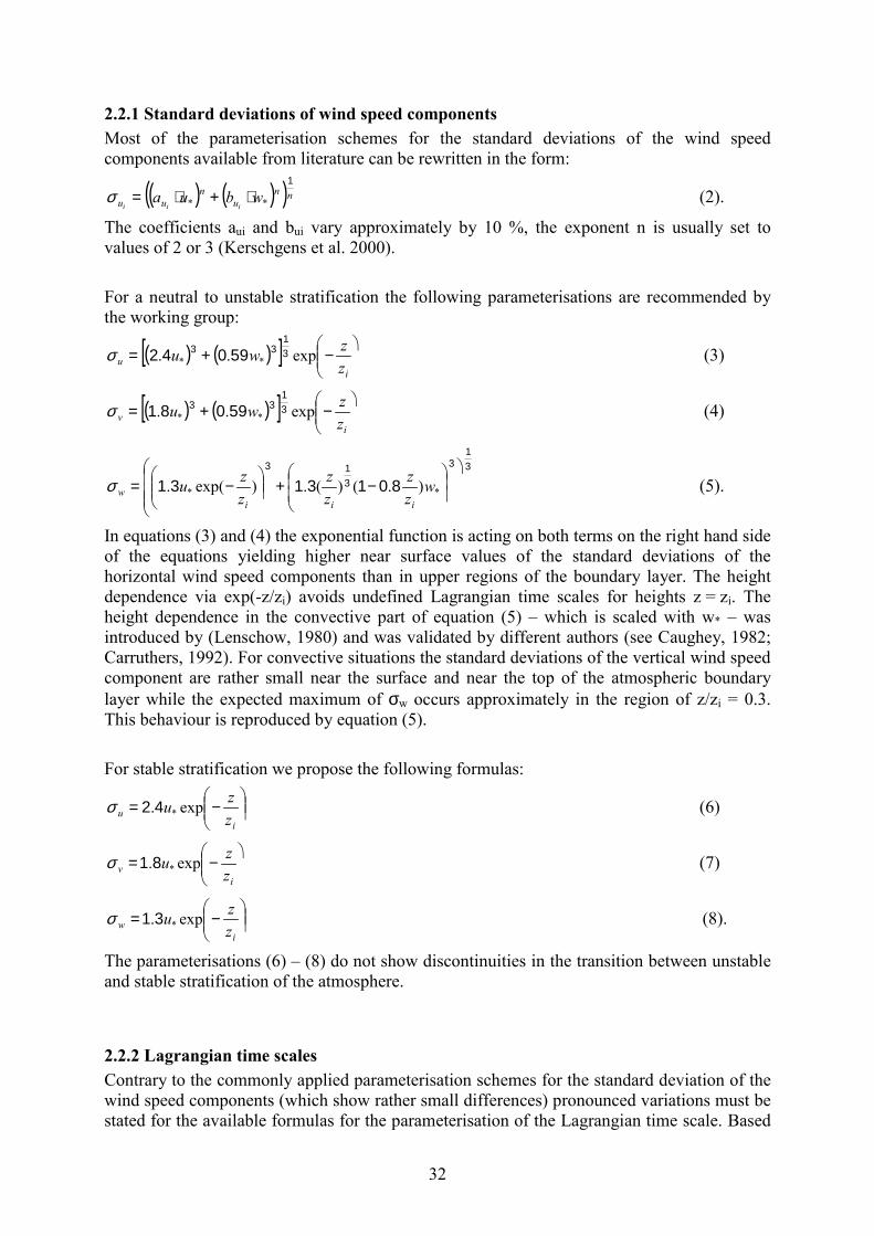
2.2.1 Standard deviations of wind speed componentsMost of the parameterisation schemes for the standard deviations of the wind speedcomponents available from literature can be rewritten in the form:

( ) ( )( )nnu

nuu wbua

iii

1

** ⋅+⋅=σ (2).

The coefficients aui and bui vary approximately by 10 %, the exponent n is usually set tovalues of 2 or 3 (Kerschgens et al. 2000).

For a neutral to unstable stratification the following parameterisations are recommended bythe working group:

( ) ( )[ ] ����

�−+=

iu z

zwu exp.. **31

33 59042σ (3)

( ) ( )[ ] ����

�−+=

iv z

zwu exp.. **31

33 59081σ (4)

31

3

313

8013131�

���

�

�

���

��

�

�−+��

����

�−= ** ).()(.)exp(. w

zz

zz

zzu

iiiwσ (5).

In equations (3) and (4) the exponential function is acting on both terms on the right hand sideof the equations yielding higher near surface values of the standard deviations of thehorizontal wind speed components than in upper regions of the boundary layer. The heightdependence via exp(-z/zi) avoids undefined Lagrangian time scales for heights z = zi. Theheight dependence in the convective part of equation (5) – which is scaled with w* – wasintroduced by (Lenschow, 1980) and was validated by different authors (see Caughey, 1982;Carruthers, 1992). For convective situations the standard deviations of the vertical wind speedcomponent are rather small near the surface and near the top of the atmospheric boundarylayer while the expected maximum of σw occurs approximately in the region of z/zi = 0.3.This behaviour is reproduced by equation (5).

For stable stratification we propose the following formulas:

���

���

�−=

iu z

zu exp. *42σ (6)

����

�−=

iv z

zu exp. *81σ (7)

���

���

�−=

iw z

zu exp. *31σ (8).

The parameterisations (6) – (8) do not show discontinuities in the transition between unstableand stable stratification of the atmosphere.

2.2.2 Lagrangian time scalesContrary to the commonly applied parameterisation schemes for the standard deviation of thewind speed components (which show rather small differences) pronounced variations must bestated for the available formulas for the parameterisation of the Lagrangian time scale. Based

33

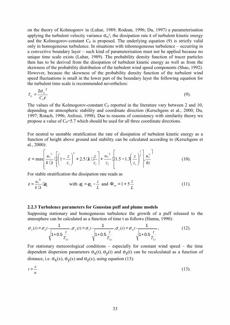
on the theory of Kolmogorov in (Luhar, 1989; Rodean, 1996; Du, 1997) a parameterisationapplying the turbulent velocity variance σui², the dissipation rate ε of turbulent kinetic energyand the Kolmogorov-constant C0 is proposed. The underlying equation (9) is strictly validonly in homogeneous turbulence. In situations with inhomogeneous turbulence – occurring ina convective boundary layer – such kind of parameterisation must not be applied because nounique time scale exists (Luhar, 1989). The probability density function of tracer particlesthen has to be derived from the dissipation of turbulent kinetic energy as well as from theskewness of the probability distribution of the turbulent wind speed components (Shao, 1992).However, because the skewness of the probability density function of the turbulent windspeed fluctuations is small in the lower part of the boundary layer the following equation forthe turbulent time scale is recommended nevertheless:

εσ

o

uL C

T i

i

22= (9).

The values of the Kolmogorov-constant C0 reported in the literature vary between 2 and 10,depending on atmospheric stability and coordinate direction (Kerschgens et al., 2000; Du,1997; Rotach, 1996; Anfossi, 1998). Due to reasons of consistency with similarity theory wepropose a value of C0=5.7 which should be used for all three coordinate directions.

For neutral to unstable stratification the rate of dissipation of turbulent kinetic energy as afunction of height above ground and stability can be calculated according to (Kerschgens etal., 2000):

�

���

�

�

����

���

�

�

���

�

�−⋅+

���

��

�

�⋅⋅+��

�

�

�−⋅

⋅=

kzu

zz

zw

zzk

zz

zku

iiii

3*

31

3*

23* ,3.15.15.21maxε (10).

For stable stratification the dissipation rate reads as

εφε ⋅⋅

=zk

u 3* with

Lz

m −=φφε and Lz

m 51+=Φ (11).

2.2.3 Turbulence parameters for Gaussian puff and plume modelsSupposing stationary and homogeneous turbulence the growth of a puff released to theatmosphere can be calculated as a function of time t as follows (Hanna, 1990):

,.

)(,.

)(,.

)(

Lz

wz

Ly

vy

Lx

ux

Tt

tt

Tt

tt

Tt

tt501

1

501

1

501

1

+=

+=

+= σσσσσσ (12).

For stationary meteorological conditions – especially for constant wind speed – the timedependent dispersion parameters σx(t),=σy(t) and σz(t) can be recalculated as a function ofdistance, i.e. σx(x),=σy(x) and σz(x), using equation (13):

uxt = (13).

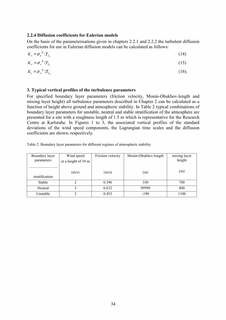
34

2.2.4 Diffusion coefficients for Eulerian modelsOn the basis of the parameterisations given in chapters 2.2.1 and 2.2.2 the turbulent diffusioncoefficients for use in Eulerian diffusion models can be calculated as follows:

uLux TK ⋅= 2σ (14)

vLvy TK ⋅= 2σ (15)

wLwz TK ⋅= 2σ (16).

3. Typical vertical profiles of the turbulence parametersFor specified boundary layer parameters (friction velocity, Monin-Obukhov-length andmixing layer height) all turbulence parameters described in Chapter 2 can be calculated as afunction of height above ground and atmospheric stability. In Table 2 typical combinations ofboundary layer parameters for unstable, neutral and stable stratification of the atmosphere arepresented for a site with a roughness length of 1.5 m which is representative for the ResearchCentre at Karlsruhe. In Figures 1 to 3, the associated vertical profiles of the standarddeviations of the wind speed components, the Lagrangian time scales and the diffusioncoefficients are shown, respectively.

Table 2: Boundary layer parameters for different regimes of atmospheric stability

Boundary layerparameters

_______________

stratification

Wind speedat a height of 10 m

(m/s)

Friction velocity

(m/s)

Monin-Obukhov-length

(m)

mixing layerheight

(m)

Stable 2 0.396 350 780Neutral 3 0.632 99999 800

Unstable 2 0.453 -190 1100

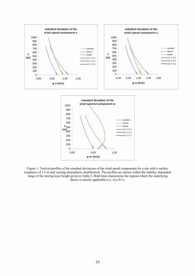
35

standard deviation of thewind speed component u

0100200300400500600700800900

1000

0,00 0,50 1,00 1,50 2,00

σσσσ -u (m/s)

z(m)

unstableneut ralstablez/zi <= 0,1z/zi <= 0,1z/zi <= 0,1

standard deviation of thewind speed component v

0100200300400500600700800900

1000

0,00 0,50 1,00 1,50

σσσσ -v (m/s)

z(m)

unstableneutralstablez/zi <= 0,1z/zi <= 0,1z/zi <= 0,1

standard deviation of thew ind speeed component w

0100200300400500

600700800900

1000

0,00 0,50 1,00σσσσ -w (m/s)

z(m)

unstableneutralstablez/zi <= 0,1z/zi <= 0,1z/zi <= 0,1

Figure 1: Vertical profiles of the standard deviations of the wind speed components for a site with a surfaceroughness of 1.5 m and varying atmospheric stratification. The profiles are shown within the stability dependent

range of the mixing layer height given in Table 2. Bold lines characterise the regions where the underlyingtheory is strictly applicable (i.e. z/zi<0.1).

36

lagrangian time scale TLu

0100200300400500600700800900

1000

0,00 100,00 200,00 300,00

TLu (s)

z(m)

unstableneutralstablez/zi <= 0,1z/zi <= 0,1z/zi <= 0,1

lagrangian time scale TLv

0100200300400500600700800900

1000

0,00 50,00 100,00 150,00

TLv (s)

z(m)

unstableneutralstablez/zi <= 0,1z/zi <= 0,1z/zi <= 0,1

lagrangian time scale TLw

0100200300400500600700800900

1000

0,00 100,00 200,00 300,00

TLw (s)

z(m)

unstableneutralstablez/zi <= 0,1z/zi <= 0,1z/zi <= 0,1

Figure 2: Vertical profiles of the lagrangian time scales for a site with a surface roughness of 1.5 m and varyingatmospheric stratification. The profiles are shown within the stability dependent range of the mixing layer height

given in Table 2. Bold lines characterise the regions where the underlying theory is strictly applicable (i.e.z/zi<0.1).

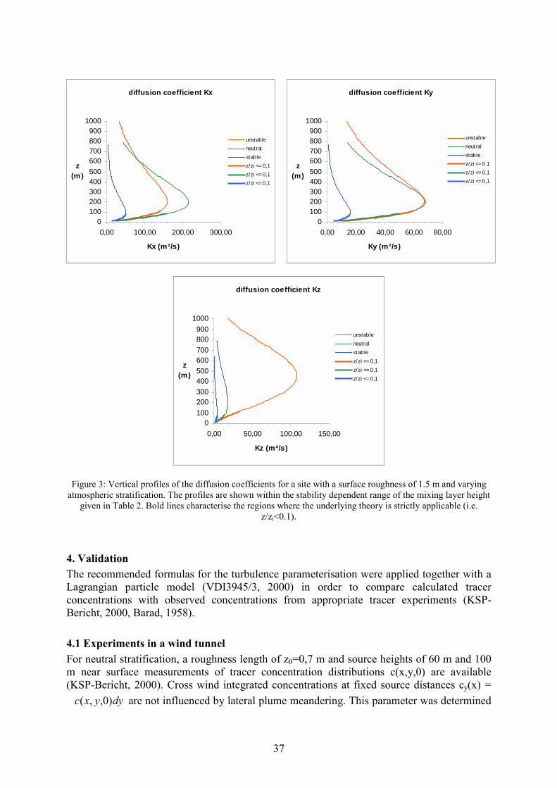
37

diffusion coefficient Kx

0100200300400500600700800900

1000

0,00 100,00 200,00 300,00

Kx (m²/s)

z(m)

unstableneutralstablez/zi <= 0,1z/zi <= 0,1z/zi <= 0,1

diffusion coefficient Ky

0100200300400500600700800900

1000

0,00 20,00 40,00 60,00 80,00

Ky (m²/s)

z(m)

unstableneutralstablez/zi <= 0,1z/zi <= 0,1z/zi <= 0,1

diffusion coefficient Kz

0100200300400500600700800900

1000

0,00 50,00 100,00 150,00

Kz (m²/s)

z(m)

unstableneutralstablez/zi <= 0,1z/zi <= 0,1z/zi <= 0,1

Figure 3: Vertical profiles of the diffusion coefficients for a site with a surface roughness of 1.5 m and varyingatmospheric stratification. The profiles are shown within the stability dependent range of the mixing layer height

given in Table 2. Bold lines characterise the regions where the underlying theory is strictly applicable (i.e.z/zi<0.1).

4. ValidationThe recommended formulas for the turbulence parameterisation were applied together with aLagrangian particle model (VDI3945/3, 2000) in order to compare calculated tracerconcentrations with observed concentrations from appropriate tracer experiments (KSP-Bericht, 2000, Barad, 1958).

4.1 Experiments in a wind tunnelFor neutral stratification, a roughness length of z0=0,7 m and source heights of 60 m and 100m near surface measurements of tracer concentration distributions c(x,y,0) are available(KSP-Bericht, 2000). Cross wind integrated concentrations at fixed source distances cy(x) =

dyyxc )0,,( are not influenced by lateral plume meandering. This parameter was determined

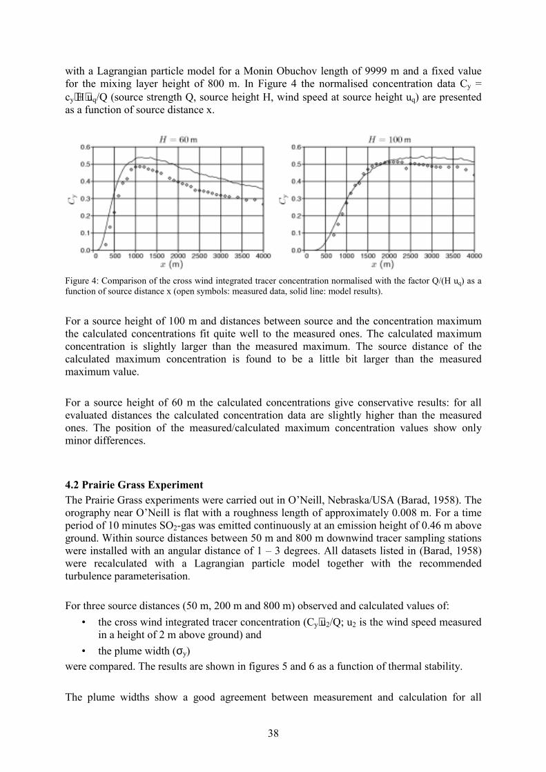
38

with a Lagrangian particle model for a Monin Obuchov length of 9999 m and a fixed valuefor the mixing layer height of 800 m. In Figure 4 the normalised concentration data Cy =cy⋅H⋅uq/Q (source strength Q, source height H, wind speed at source height uq) are presentedas a function of source distance x.

Figure 4: Comparison of the cross wind integrated tracer concentration normalised with the factor Q/(H uq) as afunction of source distance x (open symbols: measured data, solid line: model results).

For a source height of 100 m and distances between source and the concentration maximumthe calculated concentrations fit quite well to the measured ones. The calculated maximumconcentration is slightly larger than the measured maximum. The source distance of thecalculated maximum concentration is found to be a little bit larger than the measuredmaximum value.

For a source height of 60 m the calculated concentrations give conservative results: for allevaluated distances the calculated concentration data are slightly higher than the measuredones. The position of the measured/calculated maximum concentration values show onlyminor differences.

4.2 Prairie Grass ExperimentThe Prairie Grass experiments were carried out in O’Neill, Nebraska/USA (Barad, 1958). Theorography near O’Neill is flat with a roughness length of approximately 0.008 m. For a timeperiod of 10 minutes SO2-gas was emitted continuously at an emission height of 0.46 m aboveground. Within source distances between 50 m and 800 m downwind tracer sampling stationswere installed with an angular distance of 1 – 3 degrees. All datasets listed in (Barad, 1958)were recalculated with a Lagrangian particle model together with the recommendedturbulence parameterisation.

For three source distances (50 m, 200 m and 800 m) observed and calculated values of:• the cross wind integrated tracer concentration (Cy⋅u2/Q; u2 is the wind speed measured

in a height of 2 m above ground) and• the plume width (σy)

were compared. The results are shown in figures 5 and 6 as a function of thermal stability.

The plume widths show a good agreement between measurement and calculation for all

39

source distances. For unstable to neutral stratification the calculated and observed normalisedconcentration data agree very well. In cases of unstable stratification and for larger sourcedistances the differences between calculation and measurement are more pronounced. Alarger scatter in the measured data is obvious. In situations with extreme unstablestratification the tracer gas will be transported rather quickly in upper regions of theatmosphere. These convective situations can not be handled appropriately by the underlyingtheory and the recommended parameterisation respectively. In the results from dispersionmodelling a larger part of the tracer remains near the ground resulting in higher concentrationvalues.

5. ConclusionsBased on a literature study a set of formulas comprising the common understanding ofatmospheric boundary layer modelling was proposed allowing the description of atmosphericturbulence applicable for different atmospheric dispersion models based on the same synopticdataset. The recommended formulas show neither discontinuities nor jumps between differentstates of atmospheric stability as other commonly used formulas do. Comparative calculationsof tracer experiments applying a Langrangian particle model together with the recommendedturbulence parameterisation show a satisfactory level of agreement.

The formulas will be incorporated in the appendix of the amended version of the GermanTechnische Anleitung zur Reinhaltung der Luft (TA-Luft, Technical Instruction on AirQuality Control) which deals with atmospheric dispersion calculations (AUSTAL2000).

However, some (practical) problems are not yet solved. They concern the modelling of timeseries with sequences of descending mixing heights, the description of the wind profile abovezi, the modelling of dispersion inside canopy/urban canopy layer, the application to non-levelterrain, and the necessity of fixing a minimum time scale for Lagrangian particle models.Finally the universality of C0 is still an open question.

AcknowledgementsThe authors wish to thank Dr. Ulf Janicke, Ingenieurbüro Janicke, for carrying out thecalculations with the Lagrangian particle model and the comparisons with measured datapresented in Chapter 4.

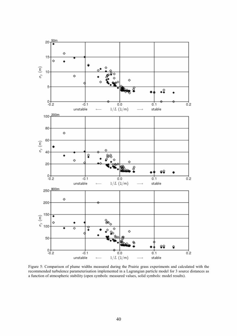
40

Figure 5: Comparison of plume widths measured during the Prairie grass experiments and calculated with therecommended turbulence parameterisation implemented in a Lagrangian particle model for 3 source distances asa function of atmospheric stability (open symbols: measured values, solid symbols: model results).

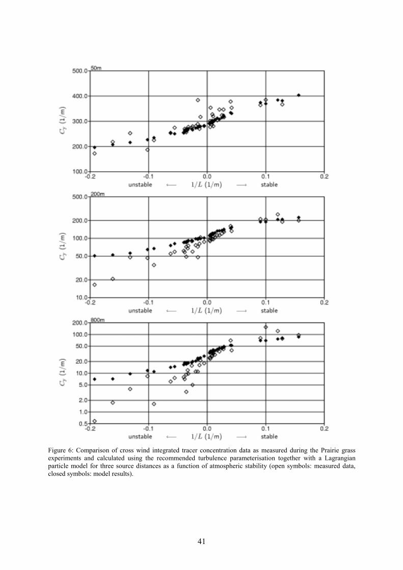
41

Figure 6: Comparison of cross wind integrated tracer concentration data as measured during the Prairie grassexperiments and calculated using the recommended turbulence parameterisation together with a Lagrangianparticle model for three source distances as a function of atmospheric stability (open symbols: measured data,closed symbols: model results).

42

References

Anfossi, D., G. Degrazia, E. Ferrero, S.E. Gryning, M.G. Morselli & S. Trini Castelli(1998). Estimation of Kolmogorov constant C0 from sonic anemometer measurements in theatmospheric surface layer. 23rd NATO/CCMS International technical meeting on air pollutionmodelling and its application, preprints, Volume II, 443 – 449.

Barad, M.L. (1958). Project Prairie Grass; a field program in diffusion; Vol. 1. GeophysicsResearch Paper No. 59, Geophysics research directorate, Air Force Cambridge ResearchCenter, Bedford, Massachusetts.

Bundesanzeiger (1990). Allgemeine Verwaltungsvorschrift zu § 45 Strahlenschutz-verordnung: Ermittlung der Strahlenexposition durch die Ableitung radioaktiver Stoffe auskerntechnischen Anlagen oder Einrichtungen. Bundesanzeiger vom 31.03.1990.

Businger, J.A. et al. (1971). Flux profile relationships in the atmospheric surface layer.Journal of the atmospheric sciences, 28, 181 - 189.

Buyn, D.W. (1990). On the analytical solution of flux profile relationships for theatmospheric surface layer. Journal of applied meteorology, 29, 652 - 657.

Carruthers, D.J., R.J. Holroyd, J.C.R. Hunt, W.S.Weng, A.G. Robins, D.D. Apsley, F.B.Smith, D.J. Thomson & B. Hudson (1992). UK Atmospheric dispersion modelling system.Air pollution modelling and its application IX (eds. H. van Dop and G. Kallos), Plenum Press,New York.

Caughey, S.J. (1982). Observed characteristics of the atmospheric boundary layer.Atmospheric turbulence and air pollution modelling (eds. Nieuwstadt, F.T.M. and H. vanDop), D. Reidel Publ..

Du, S. (1997). Universality of the Lagrangian velocity structure function constant (Co) acrossdifferent kinds of turbulence. Boundary layer meteorology, 83, 207 - 219.

GMBl (1986), Erste allgemeine Verwaltungsvorschrift zum Bundes-Immissionsschutzgesetz(Technische Anleitung zur Reinhaltung der Luft – TA Luft) vom 27.02.1986. GMBl., Ausg. A,Bonn 28.02.1986, 93 – 144.

Hanna, S.R. & D. G. Strimaitis (1990). Rugged Terrain Effects on Diffusion( Chapter 6 in:Atmospheric Processes over Complex Terrain). Meteorological Monographs, 23 (45),American Meteorological Society.

Holtslag, A.A.M. & F.T.M Nieuwstadt (1986). Scaling the atmospheric boundary layer.Boundary layer meteorology. 36, 201 - 209.

Holtslag, A.A.M. & F.T.M Nieuwstadt (1987). Reply to comments on ‘Scaling theatmospheric boundary layer‘. Boundary layer meteorology, 38, 415 - 416.

Kerschgens, M.J., C. Noelle & R. Martens (2000). Comments on turbulence parameters forthe calculation of dispersion in the atmospheric boundary layer. Meteorologische Zeitschrift,9, 155 – 163.

43

KSP-Bericht (2000). Validierung des “Kinematic Simulation Particle Model” (KSP-Modell)für Anwendungen im Vollzug des BImSchG. Meteorologisches Institut der UniversitätHamburg, Auftrag des Bundesumweltamtes, Forschungsbericht 98-295 43 354.

Lenschow, D.H. & J.C. Wyngaard (1980). Mean field and second moment budgets in abaroclinic, convective boundary layer. Journal of the atmospheric sciences, 37, 1313-1326.

Luhar, A.K. & R.E. Britter (1989). A random walk model for dispersion in inhomogeneousturbulence in a convective boundary layer. Atmospheric environment, 23, 1911-1989.

Paulson, C.A. (1970). The mathematical representation of wind speed and temperatureprofiles in the unstable atmospheric surface layer. Journal of applied meteorology, 9, 857 -861.

Rodean, H.C. (1996). Stochastic Lagrangian models of turbulent diffusion. Meteorologicalmonographs, American meteorological society, 26 (48).

Rotach, M.W., S.E. Gryning & C. Tassone (1996). A two dimensional Lagrangianstochastic dispersion model for daytime conditions. Quarterly journal of the royalmeteorological society, 122, 367 - 389.

Shao, Y. (1992). Turbulent dispersion in coastal atmospheric boundary layers: Anapplication of a Lagrangian model. Boundary layer meteorology, 59, 363-385.

van Ulden, A.P. & A.A.M. Holtslag (1985). Estimation of atmospheric boundary layerparameters for diffusion applications. Journal of Climate and Applied Meteorology, 24, 1196- 1207.

VDI3783/6 (1992). Regionale Ausbreitung von Luftverunreinigungen über komplexemGelände, Modellierung des Windfeldes 1, VDI-Handbuch Reinhaltung der Luft, Band 1,Beuth Verlag GmbH, Berlin.

VDI3945/1 (1995). Gaußsches Wolken-Modell (Puffmodell), VDI-Handbuch Reinhaltung derLuft, Band 1, Beuth Verlag GmbH, Berlin.

VDI3945/3 (2000). Atmosphärische Ausbreitungsmodelle – Partikelmodell. VDI-HandbuchReinhaltung der Luft, Band 1, Beuth Verlag GmbH, Berlin.

44

45

BUBBLE – current status of the experiment and planned investigation of theurban mixing height

Mathias W. Rotach1, Valentin Mitev2, Roland Vogt3, Alain Clappier4, Hans Richner1 and DominiqueRuffieux5

1Swiss Federal Institute of Technology, Institute for Atmospheric and Climate Science, Zürich, Switzerland2Observatory of Neuchâtel, Switzerland3University of Basel, MCR-Lab, Switzerland4Swiss Federal Institute of Technology, Laboratory of Soil and Air Pollution, Lausanne, Switzerland5MeteoSwiss, Payerne, Switzerland

Introduction

BUBBLE stands for ‘Basel UrBan Boundary Layer Experiment’ and is a research project directlyassociated to COST 715. Due to funding restrictions it has been a number of only Swiss research groupsinterested in urban meteorology (see list of authors) who have initiated this project. However, importantcommitments for contributing to the instrumentation and specific research objectives have been made bya large number of foreign institutions (Table I). While the Swiss 'core project' mainly covers the continuouslong-term observations (Section 2.3), many of the supplementary projects during periods of intensiveobservation (IOPs), will be covered by research groups from all over the world.

The philosophy of BUBBLE is based on the recognition that over complicated and essentiallyinhomogeneous urban surfaces both the near-surface turbulence exchange processes and the entireboundary layer structure have to be observed at the same time. Often in the past only detailed near-surface observations were performed over urban surfaces, without taking into consideration the largerscales (e.g., Rotach 1993, Feigenwinter et al. 1999). On the other hand, in studies dealing with the entireurban boundary layer (e.g., Argentini et al. 1999; Menut et al. 1999) the near-surface observations areoften missing or very sparse. Only in very recent urban studies such as ESCOMPTE (see F. Said, thisvolume), similar attempts as in BUBBLE were undertaken in order to combine remote sensing and near-surface in situ observations.

The present contribution summarises the observational and modelling strategies within BUBBLE andgives an overview over the mixing height determination means that will be available from the data set.

2 Observations

2.1 Near-surface sites

Two urban (‘U’), one suburban (‘S’) and a rural reference (‘R’) surface sites are presently being set up.Such a site usually consists of the following components:• Profiles up to a height larger than twice the obstacle height.• U-sites: 6 levels of sonic anemometers (some of the levels: fast response hygrometers); S- and R-

sites: 2 to 3 levels.• Full radiation balance

46

• Additional observations such as mean meteorological observations; also at the urban sites, detailedmeasurements concerning the canyon thermal and radiative properties and turbulent fluxes of CO2

are planned for short periods (IOP).

An overview of the city of Basel is shown in Fig. 1, where the sites are indicated. Additional 'industrialsites' are included for planning purposes, but the current budget and manpower doesn't allow for arealisation of those sites.

At the time of writing this report the four surface sites are being instrumented (Fig. 2 as an example) and itis expected that all of them are operational in late fall 2001.

Institution Country Area of interest Responsiblescientist

UBC Canada Radiative and thermal propertiesof street canyon

T.R. Oke

University of WesternOntario

Canada Thermal properties of streetcanyon

J. Voogt

Indiana University USA Urban energy balance C.S.B. Grimmond

Ohio State University USA Street canyon energy budget andclimate models

A.J. Arnfield

National University ofSingapore

Singapore Turbulent exchange in the urbanroughness sublayer

M. Roth

University of Tasmania Australia Radiative and thermal propertiesof street canyon

M. Nunez

Forschungs-zentrumKarlsruhe

Germany Near-surface processes; thermalstructure of urban boundary layer

N. Kalthoff

University of Freiburg Germany Urban boundary layer structure H. Mayer

TU Dresden Germany Near-surface processes Ch. Bernhofer

University of Padova Italy Near-surface processes A. PitaccoTable I Contributions to BUBBLE from institutions outside the 'core project'.

An instrument inter-comparison has been performed for some of the sonic anemometers prior to themounting of the instruments. The analysis of this data set will be performed in a similar manner as inearlier projects (Christen et al. 2000) and will allow for a distinction between measurement uncertaintiesand true physical differences in the turbulence statistics of interest.

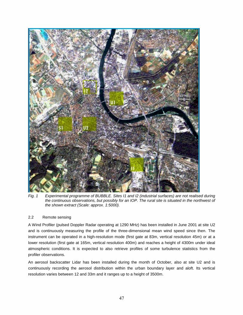
47

Fig. 1 Experimental programme of BUBBLE. Sites I1 and I2 (industrial surfaces) are not realised duringthe continuous observations, but possibly for an IOP. The rural site is situated in the northwest ofthe shown extract (Scale: approx. 1:5000).

2.2 Remote sensing

A Wind Profiler (pulsed Doppler Radar operating at 1290 MHz) has been installed in June 2001 at site U2and is continuously measuring the profile of the three-dimensional mean wind speed since then. Theinstrument can be operated in a high-resolution mode (first gate at 83m, vertical resolution 45m) or at alower resolution (first gate at 165m, vertical resolution 400m) and reaches a height of 4300m under idealatmospheric conditions. It is expected to also retrieve profiles of some turbulence statistics from theprofiler observations.

An aerosol backscatter Lidar has been installed during the month of October, also at site U2 and iscontinuously recording the aerosol distribution within the urban boundary layer and aloft. Its verticalresolution varies between 12 and 33m and it ranges up to a height of 3500m.

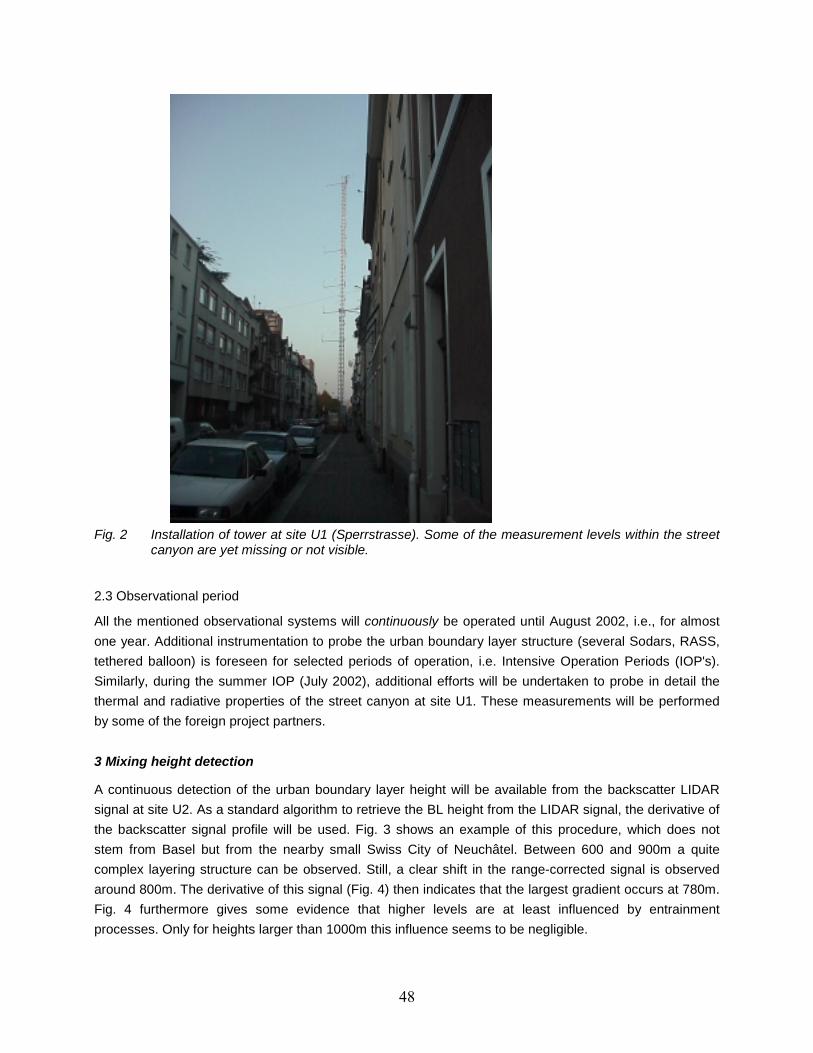
48

Fig. 2 Installation of tower at site U1 (Sperrstrasse). Some of the measurement levels within the streetcanyon are yet missing or not visible.

2.3 Observational period

All the mentioned observational systems will continuously be operated until August 2002, i.e., for almostone year. Additional instrumentation to probe the urban boundary layer structure (several Sodars, RASS,tethered balloon) is foreseen for selected periods of operation, i.e. Intensive Operation Periods (IOP's).Similarly, during the summer IOP (July 2002), additional efforts will be undertaken to probe in detail thethermal and radiative properties of the street canyon at site U1. These measurements will be performedby some of the foreign project partners.

3 Mixing height detection

A continuous detection of the urban boundary layer height will be available from the backscatter LIDARsignal at site U2. As a standard algorithm to retrieve the BL height from the LIDAR signal, the derivative ofthe backscatter signal profile will be used. Fig. 3 shows an example of this procedure, which does notstem from Basel but from the nearby small Swiss City of Neuchâtel. Between 600 and 900m a quitecomplex layering structure can be observed. Still, a clear shift in the range-corrected signal is observedaround 800m. The derivative of this signal (Fig. 4) then indicates that the largest gradient occurs at 780m.Fig. 4 furthermore gives some evidence that higher levels are at least influenced by entrainmentprocesses. Only for heights larger than 1000m this influence seems to be negligible.

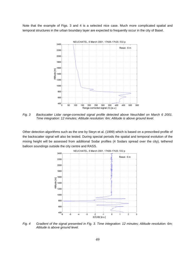
49

Note that the example of Figs. 3 and 4 is a selected nice case. Much more complicated spatial andtemporal structures in the urban boundary layer are expected to frequently occur in the city of Basel.

Fig. 3 Backscatter Lidar range-corrected signal profile detected above Neuchâtel on March 6 2001.Time integration: 12 minutes; Altitude resolution: 6m; Altitude is above ground level.

Other detection algorithms such as the one by Steyn et al. (1999) which is based on a prescribed profile ofthe backscatter signal will also be tested. During special periods the spatial and temporal evolution of themixing height will be assessed from additional Sodar profiles (4 Sodars spread over the city), tetheredballoon soundings outside the city centre and RASS.

Fig. 4 Gradient of the signal presented in Fig. 3. Time integration: 12 minutes; Altitude resolution: 6m;Altitude is above ground level.

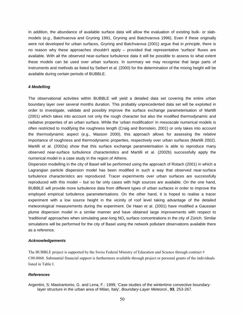
50

In addition, the abundance of available surface data will allow the evaluation of existing bulk- or slab-models (e.g., Batchvarova and Gryning 1991, Gryning and Batchvarova 1996). Even if these originallywere not developed for urban surfaces, Gryning and Batchvarova (2001) argue that in principle, there isno reason why these approaches shouldn't apply – provided that representative 'surface' fluxes areavailable. With all the observed near-surface turbulence data it will be possible to assess to what extentthese models can be used over urban surfaces. In summary we may recognise that large parts ofinstruments and methods as listed by Seibert et al. (2000) for the determination of the mixing height will beavailable during certain periods of BUBBLE.

4 Modelling

The observational activities within BUBBLE will yield a detailed data set covering the entire urbanboundary layer over several months duration. This probably unprecedented data set will be exploited inorder to investigate, validate and possibly improve the surface exchange parameterisation of Martilli(2001) which takes into account not only the rough character but also the modified thermodynamic andradiative properties of an urban surface. While the 'urban modification' in mesoscale numerical models isoften restricted to modifying the roughness length (Craig and Bornstein, 2001) or only takes into accountthe thermodynamic aspect (e.g., Masson 2000), this approach allows for assessing the relativeimportance of roughness and thermodynamic properties, respectively over urban surfaces (Martilli 2002).Martilli et al. (2002a) show that this surface exchange parameterisation is able to reproduce manyobserved near-surface turbulence characteristics and Martilli et al. (2002b) successfully apply thenumerical model in a case study in the region of Athens.Dispersion modelling in the city of Basel will be performed using the approach of Rotach (2001) in which aLagrangian particle dispersion model has been modified in such a way that observed near-surfaceturbulence characteristics are reproduced. Tracer experiments over urban surfaces are successfullyreproduced with this model – but so far only cases with high sources are available. On the one hand,BUBBLE will provide more turbulence data from different types of urban surfaces in order to improve theemployed empirical turbulence parameterisations. On the other hand, it is hoped to realise a tracerexperiment with a low source height in the vicinity of roof level taking advantage of the detailedmeteorological measurements during the experiment. De Haan et al. (2001) have modified a Gaussianplume dispersion model in a similar manner and have obtained large improvements with respect to'traditional' approaches when simulating year-long NOx surface concentrations in the city of Zürich. Similarsimulations will be performed for the city of Basel using the network pollutant observations available thereas a reference.

Acknowledgements

The BUBBLE project is supported by the Swiss Federal Ministry of Education and Science through contract #C00.0068. Substantial financial support is furthermore available through project or personal grants of the individualslisted in Table I.

References

Argentini, S; Mastrantonio, G. and Lena, F.: 1999, 'Case studies of the wintertime convective boundary-layer structure in the urban area of Milan, Italy', Boundary-Layer Meteorol., 93, 253-267.

51

Batchvarova, E. and Gryning S.E.: 1991, 'Applied model for the growth of the daytime mixed layer',Boundary-Layer Meteorol., 56 (3), 261-274.

Christen A.; van Gorsel, E; Andretta, M.; Calanca, P.; Rotach, M.W. and Vogt, R.: 2000, ‘Fieldintercomparison of ultrasonic anemometers during the MAP-Riviera project‘, Preprints NinthConference on Mountain Meteorology, August 7–11 2000, Aspen, CO, 130-131.

Craig, K.J. and Bornstein, R.D.: 2001, ' Urbanisation of Numerical Mesoscale Models', in: Rotach, M.W.;Fisher, B. and Piringer, M. (Eds.): Workshop on ‘Urban Boundary Layer Parameterisations’, COSTpublication, subm. to the European Commission, 17-30.

Feigenwinter, C.; Vogt, R. and Parlow, E.: 1999, ‘Vertical structure of selected turbulence characteristicsabove an urban canopy’, Theor. Appl. Clim., 62 (1-2), 51-63.

De Haan, P.; Rotach, M.W. and Werfeli, M: 2001, ‘Modification of an Operational Dispersion Model forUrban Applications’, J. Appl. Meteorol., 40, No 5, 864-879.

Gryning, S.-E., and Batchvarova, E.: 'Mixing heights in urban areas: will 'rural' parameterisations work?',in: Rotach, M.W.; Fisher, B. and Piringer, M. (Eds.): Workshop on ‘Urban Boundary LayerParameterisations’, COST publication, subm. to the European Commission, 99-109.

Gryning, S.-E., and Batchvarova, E.: 1996, ‘A model for the height of the internal boundary layer over anarea with an irregular coastline’, Boundary-Layer Meteorol. 78, 405-413.

Martilli, A.: 2001: ‘Development of an Urban Turbulence Parameterisation for Mesoscale AtmosphericModels’, Swiss Federal Institute of Technology Lausanne (EPFL), Dissertation # 2445, 176pp.

Martilli, A.: 2002: 'A Numerical study of the impact of an urban area on the airflow: sensitivity to synopticwind speed and urban morphology', subm. to J. Appl. Meteorol.

Martilli, A.; Clappier, A. and Rotach, M.W.: 2002a, 'A Parameterisation of the Interactions between UrbanSurfaces and the Atmosphere for Mesoscale Models', accepted Boundary-Layer Meteorology

Martilli, A.; Roulet, Y.A.; Jeunier, M.; Kirchner, F.; Rotach, M.W. and Clappier, A.: 2002b, ‘Effect of anUrban Area on Air Pollution: the Athens Case’, subm. to Atmospheric Environ.

Masson, V.: 2000, 'A physically-based scheme for the urban energy budget in atmospheric models',Boundary-Layer Meteorol., 94 (3): 357-397

Menut, L.; Flamant, C. and Pelon, J.: 1999, 'evidence of interaction between synoptic and local scales inthe surface layer over the Paris area', Boundary-Layer Meteorol., 93, 269-286.

Rotach, M.W.: 2001, ‘Simulation of urban-scale dispersion using a Lagrangian stochastic dispersionmodel’, Boundary-Layer Meteorol., 99, 379-410.

Rotach, M.W.: 1993, 'Turbulence Close to a Rough Urban Surface Part I: Reynolds Stress', Boundary-Layer Meteorol., 65, 1-28.

Seibert, P., Beyrich, F., Gryning, S-E., Joffre, S., Rasmussen, A. and Tercier, P.: 2000, 'Review andintercomparison of operational methods for the determination of the mixing height'. AtmosphericEnvironment 34, 1001-1027.

Steyn, D.G.; Baldi, M. and Hoff, R.M.: 1999, 'The detection of mixed layer depth and entrainment zonethickness from Lidar backscatter profiles', J Atmos. Oceanic Technol., 16 (7), 953-959

52

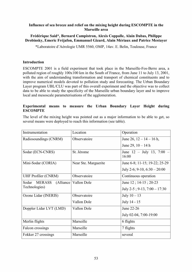
53

Influence of sea breeze and relief on the mixing height during ESCOMPTE in theMarseille area

Frédérique Said*, Bernard Campistron, Alexis Coppalle, Alain Dabas, PhilippeDrobinsky, Emeric Fréjafon, Emmanuel Gizard, Alain Mériaux and Patrice Mestayer

*Laboratoire d’Aérologie UMR 5560, OMP, 14av. E. Belin, Toulouse, France

IntroductionESCOMPTE 2001 is a field experiment that took place in the Marseille-Fos-Berre area, apolluted region of roughly 100x100 km in the South of France, from June 11 to July 13, 2001,with the aim of understanding transformation and transport of chemical constituents and toimprove numerical models devoted to pollution study and forecasting. The Urban BoundaryLayer program UBL/CLU was part of this overall experiment and the objective was to collectdata to be able to study the specificity of the Marseille urban boundary layer and to improvelocal and mesoscale parameterisations of the agglomeration.

Experimental means to measure the Urban Boundary Layer Height duringESCOMPTEThe level of the mixing height was pointed out as a major information to be able to get, soseveral means were deployed to reach this information (see table).

Instrumentation Location Operation

Radiosoundings (CNRM) Observatoire June 26, 12 – 14 – 16 h,

June 29, 10 – 14 h

Sodar (ECN-CNRS) St. Jérome June 12 – July 13, 7:00 –16:00

Mini-Sodar (CORIA) Near Ste. Marguerite June 6-8; 11-15; 19-22; 25-29

July 2-6; 9-10, 6:30 – 20:00

UHF Profiler (CNRM) Observatoire Continuous operation

Sodar MERASS (AllianceTechnologies)

Vallon Dole June 12 ; 14-15 ; 20-23

July 2-5 ; 9-13, 7:00 – 17:30

Ozone Lidar (INERIS) Observatoire

Vallon Dole

July 10 – 13

July 14 - 15

Doppler Lidar LVT (LMD) Vallon Dole June 22-26

July 02-04, 7:00-19:00

Merlin flights Marseille 6 flights

Falcon crossings Marseille 7 flights

Fokker 27 crossings Marseille several

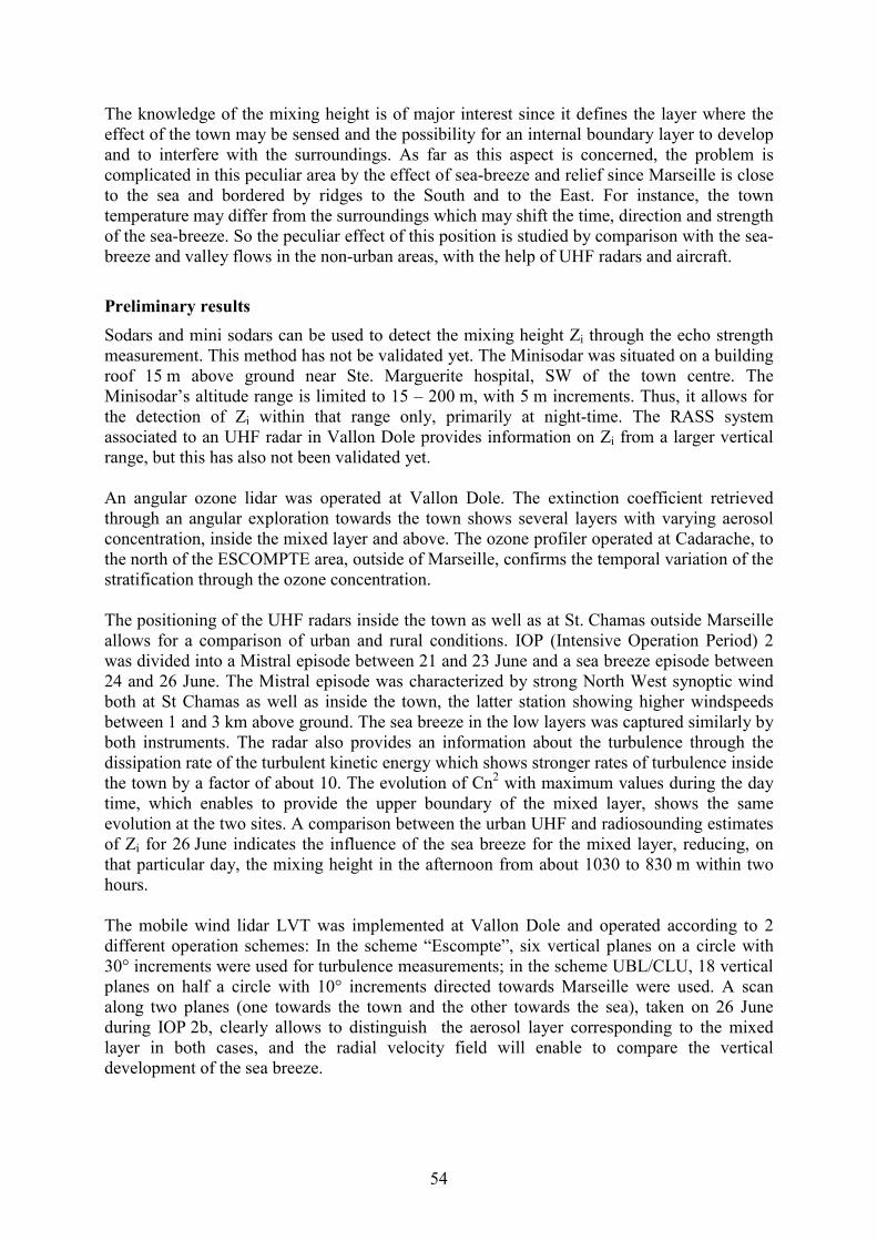
54

The knowledge of the mixing height is of major interest since it defines the layer where theeffect of the town may be sensed and the possibility for an internal boundary layer to developand to interfere with the surroundings. As far as this aspect is concerned, the problem iscomplicated in this peculiar area by the effect of sea-breeze and relief since Marseille is closeto the sea and bordered by ridges to the South and to the East. For instance, the towntemperature may differ from the surroundings which may shift the time, direction and strengthof the sea-breeze. So the peculiar effect of this position is studied by comparison with the sea-breeze and valley flows in the non-urban areas, with the help of UHF radars and aircraft.

Preliminary resultsSodars and mini sodars can be used to detect the mixing height Zi through the echo strengthmeasurement. This method has not be validated yet. The Minisodar was situated on a buildingroof 15 m above ground near Ste. Marguerite hospital, SW of the town centre. TheMinisodar’s altitude range is limited to 15 – 200 m, with 5 m increments. Thus, it allows forthe detection of Zi within that range only, primarily at night-time. The RASS systemassociated to an UHF radar in Vallon Dole provides information on Zi from a larger verticalrange, but this has also not been validated yet.

An angular ozone lidar was operated at Vallon Dole. The extinction coefficient retrievedthrough an angular exploration towards the town shows several layers with varying aerosolconcentration, inside the mixed layer and above. The ozone profiler operated at Cadarache, tothe north of the ESCOMPTE area, outside of Marseille, confirms the temporal variation of thestratification through the ozone concentration.

The positioning of the UHF radars inside the town as well as at St. Chamas outside Marseilleallows for a comparison of urban and rural conditions. IOP (Intensive Operation Period) 2was divided into a Mistral episode between 21 and 23 June and a sea breeze episode between24 and 26 June. The Mistral episode was characterized by strong North West synoptic windboth at St Chamas as well as inside the town, the latter station showing higher windspeedsbetween 1 and 3 km above ground. The sea breeze in the low layers was captured similarly byboth instruments. The radar also provides an information about the turbulence through thedissipation rate of the turbulent kinetic energy which shows stronger rates of turbulence insidethe town by a factor of about 10. The evolution of Cn2 with maximum values during the daytime, which enables to provide the upper boundary of the mixed layer, shows the sameevolution at the two sites. A comparison between the urban UHF and radiosounding estimatesof Zi for 26 June indicates the influence of the sea breeze for the mixed layer, reducing, onthat particular day, the mixing height in the afternoon from about 1030 to 830 m within twohours.

The mobile wind lidar LVT was implemented at Vallon Dole and operated according to 2different operation schemes: In the scheme “Escompte”, six vertical planes on a circle with30° increments were used for turbulence measurements; in the scheme UBL/CLU, 18 verticalplanes on half a circle with 10° increments directed towards Marseille were used. A scanalong two planes (one towards the town and the other towards the sea), taken on 26 Juneduring IOP 2b, clearly allows to distinguish the aerosol layer corresponding to the mixedlayer in both cases, and the radial velocity field will enable to compare the verticaldevelopment of the sea breeze.

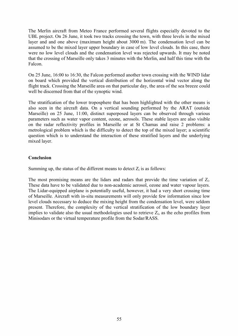
55

The Merlin aircraft from Meteo France performed several flights especially devoted to theUBL project. On 26 June, it took two tracks crossing the town, with three levels in the mixedlayer and and one above (maximum height about 3000 m). The condensation level can beassumed to be the mixed layer upper boundary in case of low level clouds. In this case, therewere no low level clouds and the condensation level was rejected upwards. It may be notedthat the crossing of Marseille only takes 3 minutes with the Merlin, and half this time with theFalcon.

On 25 June, 16:00 to 16:30, the Falcon performed another town crossing with the WIND lidaron board which provided the vertical distribution of the horizontal wind vector along theflight track. Crossing the Marseille area on that particular day, the area of the sea breeze couldwell be discerned from that of the synoptic wind.

The stratification of the lower troposphere that has been highlighted with the other means isalso seen in the aircraft data. On a vertical sounding performed by the ARAT (outsideMarseille) on 25 June, 11:00, distinct superposed layers can be observed through variousparameters such as water vapor content, ozone, aerosols. These stable layers are also visibleon the radar reflectivity profiles in Marseille or at St Chamas and raise 2 problems: ametrological problem which is the difficulty to detect the top of the mixed layer; a scientificquestion which is to understand the interaction of these stratified layers and the underlyingmixed layer.

Conclusion

Summing up, the status of the different means to detect Zi is as follows:

The most promising means are the lidars and radars that provide the time variation of Zi.These data have to be validated due to non-academic aerosol, ozone and water vapour layers.The Lidar-equipped airplane is potentially useful, however, it had a very short crossing timeof Marseille. Aircraft with in-situ measurements will only provide few information since lowlevel clouds necessary to deduce the mixing height from the condensation level, were seldompresent. Therefore, the complexity of the vertical stratification of the low boundary layerimplies to validate also the usual methodologies used to retrieve Zi, as the echo profiles fromMinisodars or the virtual temperature profile from the Sodar/RASS.

56

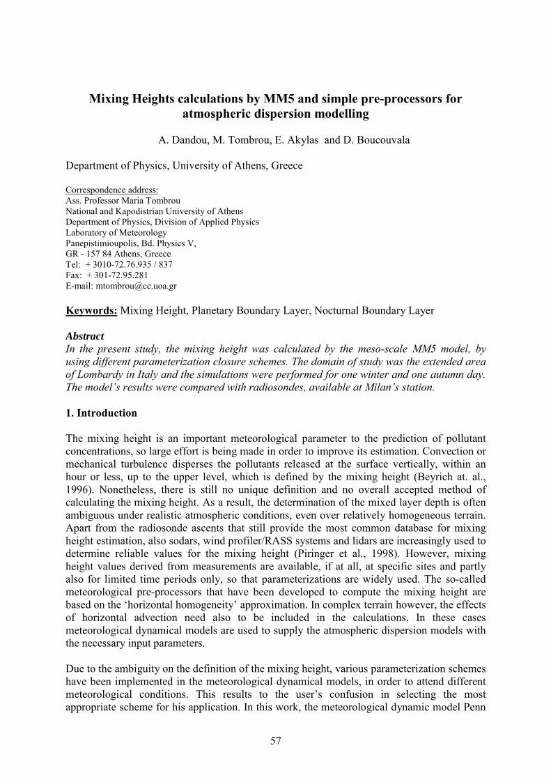
57

Mixing Heights calculations by MM5 and simple pre-processors foratmospheric dispersion modelling

A. Dandou, M. Tombrou, E. Akylas and D. Boucouvala

Department of Physics, University of Athens, Greece

Correspondence address:Ass. Professor Maria TombrouNational and Kapodistrian University of AthensDepartment of Physics, Division of Applied PhysicsLaboratory of MeteorologyPanepistimioupolis, Bd. Physics V,GR - 157 84 Athens, GreeceTel: + 3010-72.76.935 / 837Fax: + 301-72.95.281E-mail: mtombrou@cc.uoa.gr

Keywords: Mixing Height, Planetary Boundary Layer, Nocturnal Boundary Layer

AbstractIn the present study, the mixing height was calculated by the meso-scale MM5 model, byusing different parameterization closure schemes. The domain of study was the extended areaof Lombardy in Italy and the simulations were performed for one winter and one autumn day.The model’s results were compared with radiosondes, available at Milan’s station.

1. Introduction

The mixing height is an important meteorological parameter to the prediction of pollutantconcentrations, so large effort is being made in order to improve its estimation. Convection ormechanical turbulence disperses the pollutants released at the surface vertically, within anhour or less, up to the upper level, which is defined by the mixing height (Beyrich at. al.,1996). Nonetheless, there is still no unique definition and no overall accepted method ofcalculating the mixing height. As a result, the determination of the mixed layer depth is oftenambiguous under realistic atmospheric conditions, even over relatively homogeneous terrain.Apart from the radiosonde ascents that still provide the most common database for mixingheight estimation, also sodars, wind profiler/RASS systems and lidars are increasingly used todetermine reliable values for the mixing height (Piringer et al., 1998). However, mixingheight values derived from measurements are available, if at all, at specific sites and partlyalso for limited time periods only, so that parameterizations are widely used. The so-calledmeteorological pre-processors that have been developed to compute the mixing height arebased on the ‘horizontal homogeneity’ approximation. In complex terrain however, the effectsof horizontal advection need also to be included in the calculations. In these casesmeteorological dynamical models are used to supply the atmospheric dispersion models withthe necessary input parameters.

Due to the ambiguity on the definition of the mixing height, various parameterization schemeshave been implemented in the meteorological dynamical models, in order to attend differentmeteorological conditions. This results to the user’s confusion in selecting the mostappropriate scheme for his application. In this work, the meteorological dynamic model Penn

58

State/NCAR Mesoscale Model MM5 (Anthes and Warner, 1978) was used to calculate themixing height (MH) in an area with strong horizontal in-homogeneity. In particular, thevarious parameterization closure schemes, provided by the model, were tested in the greaterLombardy area in Northern Italy for both day and night on 6-2-1998 and on 12-9-1999. Themodel’s results were compared with the available radiosoundings for each day, performed inMilan’s station.

2. Models / Parameterization Schemes

The Penn State/NCAR Mesoscale Model MM5 is a numerical weather prediction model,which can be used for a broad spectrum of theoretical and real time studies, includingapplications of both predictive simulation and four-dimensional data assimilation tomonsoons, hurricanes and cyclones. On the smaller meso-beta and meso-gamma scales (2-200km), the model can be used for studies involving mesoscale convective systems, fronts, land-sea breezes, mountain-valley circulation and urban heat islands. The model can be eitherhydrostatic or non-hydrostatic.

The model includes 7 different schemes in order to parameterize the planetary boundary layerprocesses:

• Bulk PBL, based on bulk-aerodynamic parameterization, suitable for coarse verticalresolution in the boundary layer, e.g.>250m vertical grid sizes. It considers two stabilityregimes.

• High-resolution Blackadar PBL, (Zhang and Anthes, 1982), suitable for high resolutionPBL, e.g. 5 layers in the lowest km, surface layer<100m thick. Four stability regimes,including free convective mixed layer.

• Burk-Thomson PBL, based on Mellor-Yamada formulas (Burk and Thompson, 1989).Suitable for high resolution PBL. Predicts TKE (Turbulent Kinetic Energy) for use invertical mixing. It has its own force-restore ground temperature prediction.

• Eta PBL, Mellor-Yamada scheme (Janjic, 1990, 1994). It predicts TKE and has localvertical mixing.

• Gayno-Seaman PBL, based on Mellor-Yamada TKE prediction (Ballard et al., 1991). Ituses liquid-water potential temperature as a conserved variable, allowing the PBL tooperate more accurately in saturated conditions.

• MRF PBL, based on Troen-Mahrt representation for countergradient term and K profile inthe well mixed PBL (Hong and Pan, 1996)

• Pleim-Chang PBL, the Asymmetric Convective Model, using a variation on Blackadar’snon-local vertical mixing (Pleim and Chang, 1992)

The first 5 schemes are based on local parameters while the last 2 involve non-localparameters and are considered more suitable for strongly unstable conditions.

3. PBL calculations with different parameterization schemes

The area, where we applied the model, is the greater Lombardy area in Northern Italy (Fig.1).The area of interest is the 2nd nested domain in the model. At the borders the boundaryconditions provided by the 1st domain prevail. Thus, the values at the edges are expected tohave lower reliability. The model runs continuously for one winter day, the 6th of February1998 and one autumn day, the 12th of September 1999, for each one of the selectedparameterization schemes. In this particular study the MRF, the High-resolution Blackadar

59

and the Gayno-Seaman parameterization schemes were applied with the version V3-4 of theMM5 model.

The model’s simulations show a homogeneous mixing height in the basin, which is wellexplained by the hour of the calculation. In the mountainous area, both North and South of thedomain, the mixing height strongly varies following the local topography. The maximumvalues of mixing heights were calculated above the mountain crests. In particular, for thewinter day the values of mixing heights at the basin, provided by the local parameterizationschemes, were the lowest. For the Blackadar scheme (Fig. 2) the heights reach altitudes of250-300m, while for the Gayno-Seaman (Fig. 3) they are up to 200-250m. The correspondingvalues, provided by the MRF non-local scheme, were much higher, up to 400-500m (Fig. 4).During the autumn day the mixing heights were estimated substantially larger in accordancewith the atmospheric conditions that were prevailing in the basin. The local scheme ofBlackadar indicated values around 1100-1300m (Fig.5) while the MRF showed values up to1800-2000m (Fig.6). During the night the two non-local schemes give almost zero values ofthe mixing height for both days, while the MRF scheme gives values around 50m on thewinter day and around 100-150m on the autumn day. In Figs. 1 to 6, the numbers on both axesrefer to grid cell numbers. The (x 2km) refers to the resolution of the grid cell.

Thereafter, the calculated diurnal variation of the mixing height by using different PBLparameterization schemes (Fig 7 and 9) is compared with the available radiosoundings, takenfrom Milan, for both days. The potential temperature profiles taken from Milan’s station aregiven in Figures 8 and 10. It should be mentioned that the height presented in theradiosoundings is Above Sea Level (ASL), so the station’s elevation (103m) should beabstracted in order to compare the model’s results with the inversion height.

The estimation of mixing heights from the radiosoundings was performed using a techniquesuggested by Heffter (1980). In this method, potential temperature profiles are computed foreach sounding. The profiles are analyzed for the existence of a ‘critical inversion’, which isassumed to mark the top of the mixed layer. In this scheme, a critical inversion is defined asthe lowest inversion that meets the following two criteria:

1005.0 −≥∆∆ KmZθ (1)Kbasetop 2≥−θθ (2)

where Z∆∆θ is the potential temperature lapse rate in the inversion layer and topθ and baseθrefer to the potential temperatures at the top and bottom of the critical inversion layer. Theheight of the mixing layer is that point in the inversion layer at which the temperature is 2oKabove the temperature at the inversion base. This method was selected for use because itrecognizes the likelihood of mixing (caused by buoyant thermals) to overshoot the base of thecritical inversion. This physical process is overlooked in many similar schemes. This schemehas also been considered in the studies of Marsik et al., 1995 and Piringer et al., 1998.

On 6-2-1998 a mixing height of 379m ASL at 12:00 UT is deduced from the potentialtemperature profile (Fig. 8), based on the method described above. This value is in relativegood accordance with the Blackadar scheme (Fig. 7). During the night a temperatureinversion is apparent; thus, the development of mixing height can only be attributed to thewind shear. The value of 50m provided by the MRF scheme is considered more reliable thanthe zero value, calculated by the other two local schemes. On the autumn day, the mixingheight derived from the potential temperature’s profile (Fig. 10), using the same method, is upto 1980m ASL at 12:00 UT. This is in good agreement with the values calculated by the MRF

60

scheme, as presented in Figure 9. During the night, the non-local MRF scheme gives a mixingheight up to 100m (Fig. 9), which is also in good relation with the radiosounding’s inversionheight.

4. Conclusions-Future work

From the limited results presented above, it is apparent that during strong convection the MRFseems to be the most appropriate closure scheme. However, during the winter day it seems tooverestimate the mixing height. The nocturnal mixing height, which depicts the layer wherethe pollutants are blended, is poorly predicted by the examined schemes.

Further to the above work, an effort is made to implement current advanced parameterizationschemes (Zilitinkevich et al., 1998, Akylas et al., 2001) into the model. In particular we focuson the strongly unstable regimes over rough areas.

Especially for the Nocturnal Boundary Layer (NBL), the work will be continued with thecollaboration with San Jose University. The area under investigation is the basin of LosAngeles, where datasets of surface measurements from 110 surface sites, performed duringthe Southern California Ozone Study (SCOS97) as well as data from profilers andrawinsondes are available. Moreover, the simple meteorological pre-processors addressed forthe Nocturnal Boundary Layer, (Tombrou et al., 1998) will be applied in the Los Angelesbasin for the 4-7 August 1997. In this case, the calculations of mixing heights will beperformed by considering two sets of data, separately: a) surface measurements and b) theatmospheric parameters calculated by the MM5 model, with the Mellor-Yamadaparameterization scheme (Ballard et al., 1991). Thereafter, the resulting NBL values will becompared to vertical measured data (profilers and rawinsondes) through the maximum windsand inversion heights as well as to the theoretical calculations from the MM5 model.

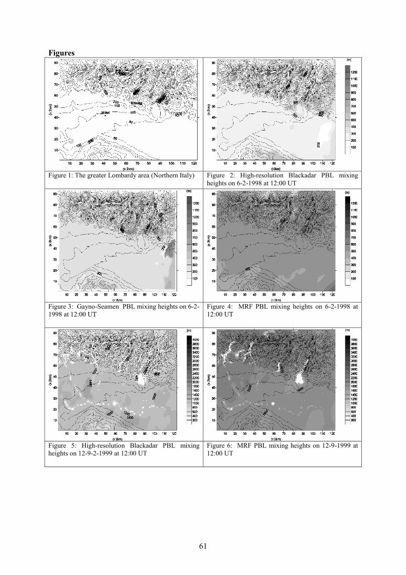
61

Figures

Figure 1: The greater Lombardy area (Northern Italy) Figure 2: High-resolution Blackadar PBL mixingheights on 6-2-1998 at 12:00 UT

Figure 3: Gayno-Seamen PBL mixing heights on 6-2-1998 at 12:00 UT

Figure 4: MRF PBL mixing heights on 6-2-1998 at12:00 UT

Figure 5: High-resolution Blackadar PBL mixingheights on 12-9-2-1999 at 12:00 UT

Figure 6: MRF PBL mixing heights on 12-9-1999 at12:00 UT

62

0

50

100

150

200

250

300

350

400

450

500

0 2 4 6 8 10 12 14 16 18 20 22 24

time (h)

mix

ing

heig

ht (m

)

BlackadarGanyo-SeamanMRF

Figure 7: Diurnal variation of mixing height with differnet PBL schemes in Milan on 6-2-1998

0

250

500

750

1000

1250

1500

1750

2000

2250

2500

270 275 280 285 290Temperature (oK)

heig

ht (m

ASL

)

Figure 8: Potential temperature profiles taken from Milan’s station on 6-2-1998 at a) 0:00 UT ( ) b) 6:00 UT( ) and c) 12:00 UT ( )

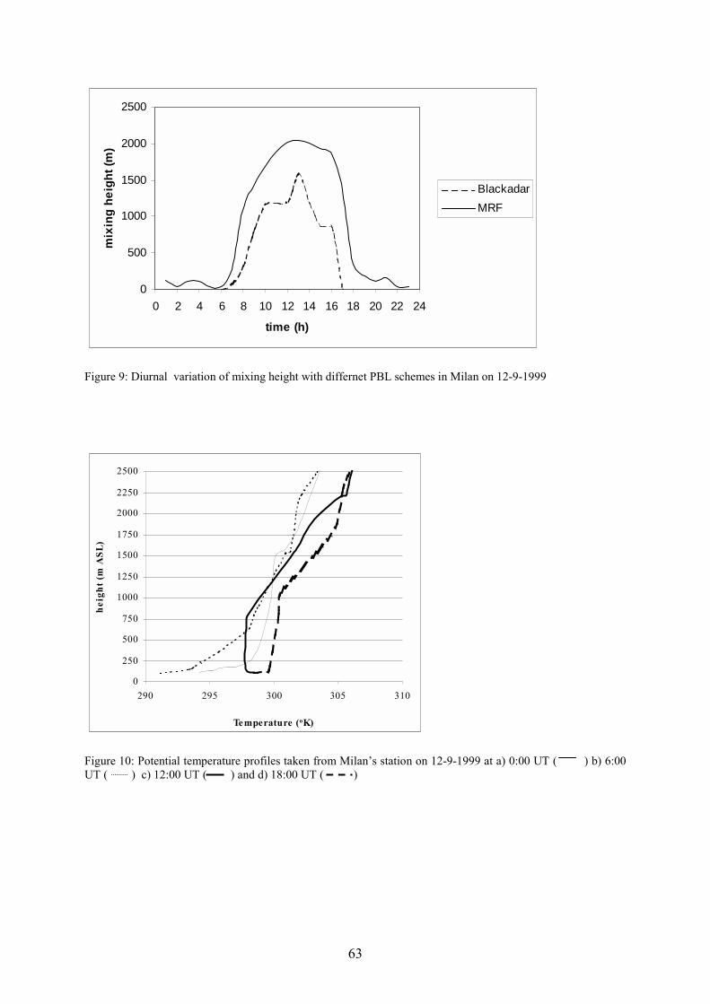
63

0

500

1000

1500

2000

2500

0 2 4 6 8 10 12 14 16 18 20 22 24

time (h)

mix

ing

heig

ht (m

)

BlackadarMRF

Figure 9: Diurnal variation of mixing height with differnet PBL schemes in Milan on 12-9-1999

0

250

500

750

1000

1250

1500

1750

2000

2250

2500

290 295 300 305 310

Temperature (oK)

heig

ht (m

ASL

)

Figure 10: Potential temperature profiles taken from Milan’s station on 12-9-1999 at a) 0:00 UT ( ) b) 6:00UT ( ) c) 12:00 UT ( ) and d) 18:00 UT ( )

64

References

Akylas, E., M. Tombrou, D. Lalas, and S. Zilitinkevich, (2001a). ‘Surface fluxes under shear-free convection’. Quart. J. Roy. Meteorol. Soc., 127, pp.1-15.

Anthes, R.A. and Warner, T.T., (1978). ‘Development of hydrodynamic models suitable forair pollution and other meso-meteorological studies’, Mon. Wea. Rev., 106, pp. 1045-1078.

Ballard, S.P., Golding B.W. and Smith R.N., (1991). ‘Mesoscale model experimentalForecasts of the Haar of Northeast Scotland’, Mon. Wea. Rev., 119, pp. 2107-2123.

Beyrich, F., Gryning, S.E., Joffre, S., Rasmussen, A., Seibert, P. and Tercier, P., (1996). ‘Onthe Determination of mixing Height: A Review’, Proc. of the 4th Workshop on Harmonisationwithin Atmospheric Dispersion Modelling for Regulatory Purposes, 6-9 May 1996, Oostende,Belgium, pp. 155-162.

Burk S. D. and Thomson W.T., (1989). ‘A vertically nested regional numerical predictionmodel with second order closure physics’. Mon. Wea. Rev., 117, pp. 2305-2324.

Heffter J. L., (1980). ‘Air resources laboratories atmospheric transport and dispersionmodel’. NOAA Tech. Memo. ERL ARL -81, pp.24.

Hong S.-Y. and Pan H.-L., (1996). ‘Nonlocal boundary layer vertical diffusion in a medium-range forecast model’. Mon. Wea. Rev., 124, pp. 2322-2339.

Janjinc Zavisa I., (1994). ‘The step-mountain eta coordinate model: Further development ofthe convection, viscous sublayer and turbulent closure schemes’. Mon. Wea. Rev., 122,pp.927-945.

Marsik F.J., Kenneth W.F., Tracey D.M., Perry J.S., (1995). ‘Comparison of Methods forEstimating Mixing height Used during the 1992 Atlanta Field Intensive’, J. Appl. Meteor., 34,pp. 1802-1814.

Pleim J.E. and Chang J.S., (1992). ‘A non local model for vertical mixing in the convectiveboundary layer’, Atmos. Environ., 26A, pp. 965-981.

Piringer, M., Baumann K. and Langer, M., (1998). ‘Summertime mixing heights at Vienna,Austria, estimated from vertical soundings and by a numerical model’, Boundary-LayerMeteorol., 89, pp. 25-45.

Tombrou M., E. Founda and D. Boucouvala, (1998).‘Nocturnal boundary layer heightprediction from surface routine meteorological data’, Meteorology and Atmospheric Physics,68, pp.77-186.

Zhang D. and Anthes R.A., (1982).‘Nocturnal boundary layer height prediction from surfaceroutine meteorological data’, J. Appl. Meteor., 21, pp.1594-1609.

65

Analysis of Air Pollution Episodes in European Cities

Ranjeet S Sokhi1, Lakhu Luhana1, Jaakko Kukkonen2, Erik Berge3,Leiv Harvard Slördal4 and Sandro Finardi5

1. ASRG, Department of Environmental Sciences, University of Hertfordshire,Hatfield, AL10 9AB, UK

2. Finnish Meteorological Institute FMI, Air Quality Research,Sahaajankatu 20 E, FIN-00880 Helsinki, FINLAND3. The Norwegian Meteorological Institute DNMI,Postboks 43, Blindern, N-0313 Oslo, NORWAY

4. The Norwegian Institute for Air Research NILU,Instituttvn 18, PO Box 100, N-2027 Kjeller, NORWAY

5. ARIANET, viale Elvezia 42, 20052 Monza (MI), ITALY

Abstract

This paper reports on the preliminary analysis of air pollution episodes in severalEuropean cities: London, Oslo, Milan and Helsinki. Examples of episodes of PM10,NO2 and O3 are presented and the causes are examined in relation to local emissionsand meteorological conditions. Similarities and differences in relation to theimportance of meteorological conditions including inversions are discussed for thesemajor urban regions. The frequency of low wind speed (< 2 m/s) conditions issignificant in all of these cities; for example, in London and Helsinki these frequencesare typically of the order of 25 and 45 %, respectively. For both particulate matter andnitrogen oxides, low lying inversion and low wind speeds are particularly important inthat they tend to lead to high concentration of air pollutants. In the case of PM10episodes, sources such as wood burning and resuspended particulate matter fromstreet surfaces are important in Northern European cities, such as Oslo and Helsinki.Within the UK, studies have indicated that PM10 episodes have been caused by airmasses bringing high loadings of secondary particles. For NO2, measurements at threesites within London registered daily averaged concentrations above 200 µg/m3 duringDecember 1994. Hourly maximum value during this period at London Bloomsburyshowed concentrations reaching 400 µg/m3 whilst the wind speeds were at or below 1m/s. In Milan, episodes of NO2 are common during anticyclonic conditions withpersistent weak wind fields.

1. Introduction

This paper forms part of the work of the COST 715 action "Meteorology Applied toUrban Air Pollution Problems" (e.g., Fisher et al., 2001). It is produced within theabove-mentioned action by Working Group 3 “Meteorology during peak pollutionepisodes”. This paper aims to undertake a preliminary analysis of episodes of PM10,NO2 and O3 in four selected European cities, London, Oslo, Milan and Helsinki.

Air pollution episodes in and around cities can pose a serious hazard to human health.Under episodic conditions concentrations of air pollutants such as O3, NO2 andparticulate matter (measured, e.g., as the mass fractions PM10 and PM2.5) canconsiderably exceed national and international standards and limit values (e.g.,

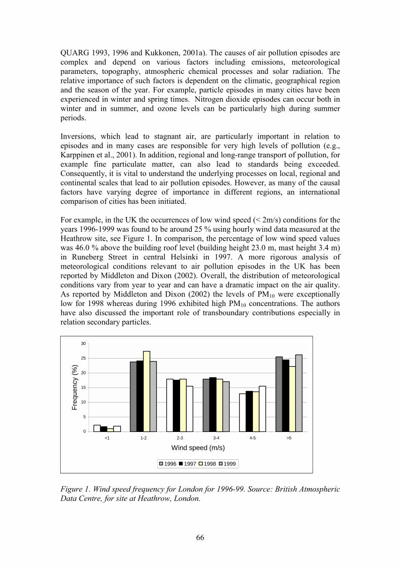
66

QUARG 1993, 1996 and Kukkonen, 2001a). The causes of air pollution episodes arecomplex and depend on various factors including emissions, meteorologicalparameters, topography, atmospheric chemical processes and solar radiation. Therelative importance of such factors is dependent on the climatic, geographical regionand the season of the year. For example, particle episodes in many cities have beenexperienced in winter and spring times. Nitrogen dioxide episodes can occur both inwinter and in summer, and ozone levels can be particularly high during summerperiods.

Inversions, which lead to stagnant air, are particularly important in relation toepisodes and in many cases are responsible for very high levels of pollution (e.g.,Karppinen et al., 2001). In addition, regional and long-range transport of pollution, forexample fine particulate matter, can also lead to standards being exceeded.Consequently, it is vital to understand the underlying processes on local, regional andcontinental scales that lead to air pollution episodes. However, as many of the causalfactors have varying degree of importance in different regions, an internationalcomparison of cities has been initiated.

For example, in the UK the occurrences of low wind speed (< 2m/s) conditions for theyears 1996-1999 was found to be around 25 % using hourly wind data measured at theHeathrow site, see Figure 1. In comparison, the percentage of low wind speed valueswas 46.0 % above the building roof level (building height 23.0 m, mast height 3.4 m)in Runeberg Street in central Helsinki in 1997. A more rigorous analysis ofmeteorological conditions relevant to air pollution episodes in the UK has beenreported by Middleton and Dixon (2002). Overall, the distribution of meteorologicalconditions vary from year to year and can have a dramatic impact on the air quality.As reported by Middleton and Dixon (2002) the levels of PM10 were exceptionallylow for 1998 whereas during 1996 exhibited high PM10 concentrations. The authorshave also discussed the important role of transboundary contributions especially inrelation secondary particles.

Figure 1. Wind speed frequency for London for 1996-99. Source: British AtmosphericData Centre, for site at Heathrow, London.

0

5

10

15

20

25

30

<1 1-2 2-3 3-4 4-5 >5

Wind speed (m/s)

Freq

uenc

y (%

)

1996 1997 1998 1999

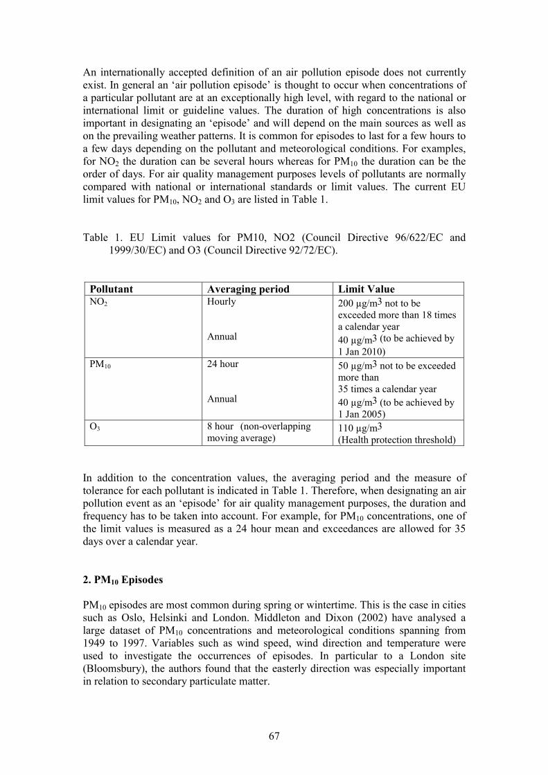
67

An internationally accepted definition of an air pollution episode does not currentlyexist. In general an ‘air pollution episode’ is thought to occur when concentrations ofa particular pollutant are at an exceptionally high level, with regard to the national orinternational limit or guideline values. The duration of high concentrations is alsoimportant in designating an ‘episode’ and will depend on the main sources as well ason the prevailing weather patterns. It is common for episodes to last for a few hours toa few days depending on the pollutant and meteorological conditions. For examples,for NO2 the duration can be several hours whereas for PM10 the duration can be theorder of days. For air quality management purposes levels of pollutants are normallycompared with national or international standards or limit values. The current EUlimit values for PM10, NO2 and O3 are listed in Table 1.

Table 1. EU Limit values for PM10, NO2 (Council Directive 96/622/EC and1999/30/EC) and O3 (Council Directive 92/72/EC).

Pollutant Averaging period Limit ValueNO2 Hourly

Annual

200 µg/m3 not to beexceeded more than 18 timesa calendar year40 µg/m3 (to be achieved by1 Jan 2010)

PM10 24 hour

Annual

50 µg/m3 not to be exceededmore than35 times a calendar year40 µg/m3 (to be achieved by1 Jan 2005)

O3 8 hour (non-overlappingmoving average)

110 µg/m3(Health protection threshold)

In addition to the concentration values, the averaging period and the measure oftolerance for each pollutant is indicated in Table 1. Therefore, when designating an airpollution event as an ‘episode’ for air quality management purposes, the duration andfrequency has to be taken into account. For example, for PM10 concentrations, one ofthe limit values is measured as a 24 hour mean and exceedances are allowed for 35days over a calendar year.

2. PM10 Episodes

PM10 episodes are most common during spring or wintertime. This is the case in citiessuch as Oslo, Helsinki and London. Middleton and Dixon (2002) have analysed alarge dataset of PM10 concentrations and meteorological conditions spanning from1949 to 1997. Variables such as wind speed, wind direction and temperature wereused to investigate the occurrences of episodes. In particular to a London site(Bloomsbury), the authors found that the easterly direction was especially importantin relation to secondary particulate matter.

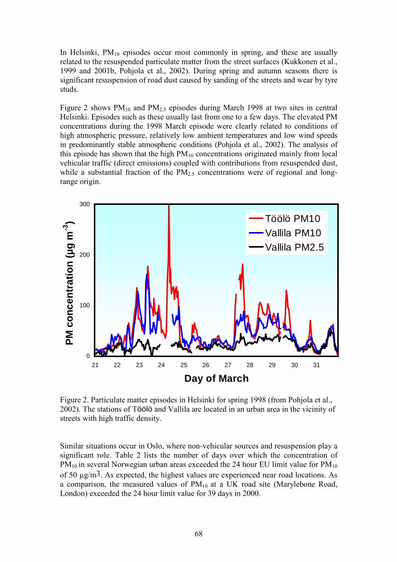
68

In Helsinki, PM10 episodes occur most commonly in spring, and these are usuallyrelated to the resuspended particulate matter from the street surfaces (Kukkonen et al.,1999 and 2001b, Pohjola et al., 2002). During spring and autumn seasons there issignificant resuspension of road dust caused by sanding of the streets and wear by tyrestuds.

Figure 2 shows PM10 and PM2.5 episodes during March 1998 at two sites in centralHelsinki. Episodes such as these usually last from one to a few days. The elevated PMconcentrations during the 1998 March episode were clearly related to conditions ofhigh atmospheric pressure, relatively low ambient temperatures and low wind speedsin predominantly stable atmospheric conditions (Pohjola et al., 2002). The analysis ofthis episode has shown that the high PM10 concentrations originated mainly from localvehicular traffic (direct emissions) coupled with contributions from resuspended dust,while a substantial fraction of the PM2.5 concentrations were of regional and long-range origin.

Figure 2. Particulate matter episodes in Helsinki for spring 1998 (from Pohjola et al.,2002). The stations of Töölö and Vallila are located in an urban area in the vicinity ofstreets with high traffic density.

Similar situations occur in Oslo, where non-vehicular sources and resuspension play asignificant role. Table 2 lists the number of days over which the concentration ofPM10 in several Norwegian urban areas exceeded the 24 hour EU limit value for PM10

of 50 µg/m3. As expected, the highest values are experienced near road locations. Asa comparison, the measured values of PM10 at a UK road site (Marylebone Road,London) exceeded the 24 hour limit value for 39 days in 2000.

0

100

200

300

21 22 23 24 25 26 27 28 29 30 31

Day of March

PM c

once

ntra

tion

(µg

m-3

) Töölö PM10Vallila PM10Vallila PM2.5

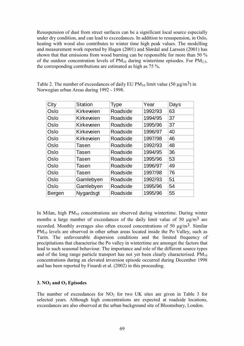
69

Resuspension of dust from street surfaces can be a significant local source especiallyunder dry condition, and can lead to exceedances. In addition to resuspension, in Oslo,heating with wood also contributes to winter time high peak values. The modellingand measurement work reported by Hagen (2001) and Slørdal and Larssen (2001) hasshown that that emissions from wood burning can be responsible for more than 50 %of the outdoor concentration levels of PM10 during wintertime episodes. For PM2.5,the corresponding contributions are estimated as high as 75 %.

Table 2. The number of exceedances of daily EU PM10 limit value (50 µg/m3) inNorwegian urban Areas during 1992 - 1998.

In Milan, high PM10 concentrations are observed during wintertime. During wintermonths a large number of exceedances of the daily limit value of 50 µg/m3 arerecorded. Monthly averages also often exceed concentrations of 50 µg/m3. SimilarPM10 levels are observed in other urban areas located inside the Po Valley, such asTurin. The unfavourable dispersion conditions and the limited frequency ofprecipitations that characterise the Po valley in wintertime are amongst the factors thatlead to such seasonal behaviour. The importance and role of the different source typesand of the long range particle transport has not yet been clearly characterised. PM10concentrations during an elevated inversion episode occurred during December 1998and has been reported by Finardi et al. (2002) in this proceeding.

3. NO2 and O3 Episodes

The number of exceedances for NO2 for two UK sites are given in Table 3 forselected years. Although high concentrations are expected at roadside locations,exceedances are also observed at the urban background site of Bloomsbury, London.

City Station Type Year DaysOslo Kirkeveien Roadside 1992/93 63Oslo Kirkeveien Roadside 1994/95 37Oslo Kirkeveien Roadside 1995/96 37Oslo Kirkeveien Roadside 1996/97 40Oslo Kirkeveien Roadside 1997/98 46Oslo Tasen Roadside 1992/93 48Oslo Tasen Roadside 1994/95 36Oslo Tasen Roadside 1995/96 53Oslo Tasen Roadside 1996/97 49Oslo Tasen Roadside 1997/98 76Oslo Gamlebyen Roadside 1992/93 51Oslo Gamlebyen Roadside 1995/96 54Bergen Nygardsgt Roadside 1995/96 55

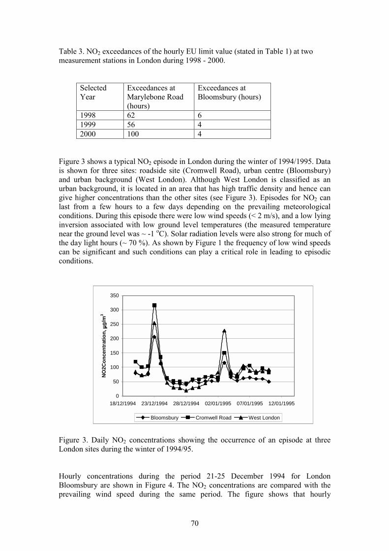
70

Table 3. NO2 exceedances of the hourly EU limit value (stated in Table 1) at twomeasurement stations in London during 1998 - 2000.

SelectedYear

Exceedances atMarylebone Road(hours)

Exceedances atBloomsbury (hours)

1998 62 61999 56 42000 100 4

Figure 3 shows a typical NO2 episode in London during the winter of 1994/1995. Datais shown for three sites: roadside site (Cromwell Road), urban centre (Bloomsbury)and urban background (West London). Although West London is classified as anurban background, it is located in an area that has high traffic density and hence cangive higher concentrations than the other sites (see Figure 3). Episodes for NO2 canlast from a few hours to a few days depending on the prevailing meteorologicalconditions. During this episode there were low wind speeds (< 2 m/s), and a low lyinginversion associated with low ground level temperatures (the measured temperaturenear the ground level was ~ -1 oC). Solar radiation levels were also strong for much ofthe day light hours (~ 70 %). As shown by Figure 1 the frequency of low wind speedscan be significant and such conditions can play a critical role in leading to episodicconditions.

Figure 3. Daily NO2 concentrations showing the occurrence of an episode at threeLondon sites during the winter of 1994/95.

Hourly concentrations during the period 21-25 December 1994 for LondonBloomsbury are shown in Figure 4. The NO2 concentrations are compared with theprevailing wind speed during the same period. The figure shows that hourly

0

50

100

150

200

250

300

350

18/12/1994 23/12/1994 28/12/1994 02/01/1995 07/01/1995 12/01/1995

NO2C

once

ntra

tion,

µµ µµg/

m3

Bloomsbury Cromwell Road West London

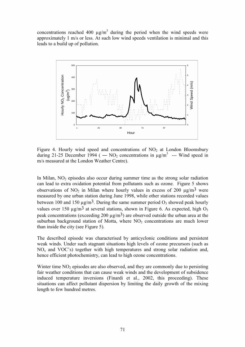
71

concentrations reached 400 µg/m3 during the period when the wind speeds wereapproximately 1 m/s or less. At such low wind speeds ventilation is minimal and thisleads to a build up of pollution.

Figure 4. Hourly wind speed and concentrations of NO2 at London Bloomsburyduring 21-25 December 1994 ( ― NO2 concentrations in µg/m3 --- Wind speed inm/s measured at the London Weather Centre).

In Milan, NO2 episodes also occur during summer time as the strong solar radiationcan lead to extra oxidation potential from pollutants such as ozone. Figure 5 showsobservations of NO2 in Milan where hourly values in excess of 200 µg/m3 weremeasured by one urban station during June 1998, while other stations recorded valuesbetween 100 and 150 µg/m3. During the same summer period O3 showed peak hourlyvalues over 150 µg/m3 at several stations, shown in Figure 6. As expected, high O3

peak concentrations (exceeding 200 µg/m3) are observed outside the urban area at thesuburban background station of Motta, where NO2 concentrations are much lowerthan inside the city (see Figure 5).

The described episode was characterised by anticyclonic conditions and persistentweak winds. Under such stagnant situations high levels of ozone precursors (such asNOx and VOC’s) together with high temperatures and strong solar radiation and,hence efficient photochemistry, can lead to high ozone concentrations.

Winter time NO2 episodes are also observed, and they are commonly due to persistingfair weather conditions that can cause weak winds and the development of subsidenceinduced temperature inversions (Finardi et al., 2002, this proceeding). Thesesituations can affect pollutant dispersion by limiting the daily growth of the mixinglength to few hundred metres.

0

100

200

300

400

500

1 25 49 73 97

Hour

Hou

rly N

O2 C

once

ntra

tion

(ug/

m3 )

0

1

2

3

4

5

6

Win

d Sp

eed

(m/s

)

72

01/06/98 02/06/98 03/06/98 04/06/98 05/06/98 06/06/98 07/06/98

Date

100

200

300N

O2(µg

/m3 )

Juvara - UrbanVerziere - Urban RoadsidePco Lambro - Urban ParkMotta - Suburban Background

Milan City Air Quality ControlNetwork - NO2

Figure 5. The NO2 concentrations measured at four stations during an episode inMilan area for June 1998.

01/06/98 02/06/98 03/06/98 04/06/98 05/06/98 06/06/98 07/06/98

Date

100

200

300

O3(µg

/m3 )

Milan City Air Quality ControlNetwork - O3

Figure 6. Ozone concentrations measured at the same four stations (as in Figure 5) inMilan during June 1998.

Conclusions

The causes of air pollution episodes depend on several factors including local andregional emissions, topography and meteorological parameters including wind speed,wind direction, temperature and solar radiation. The relative importance of such

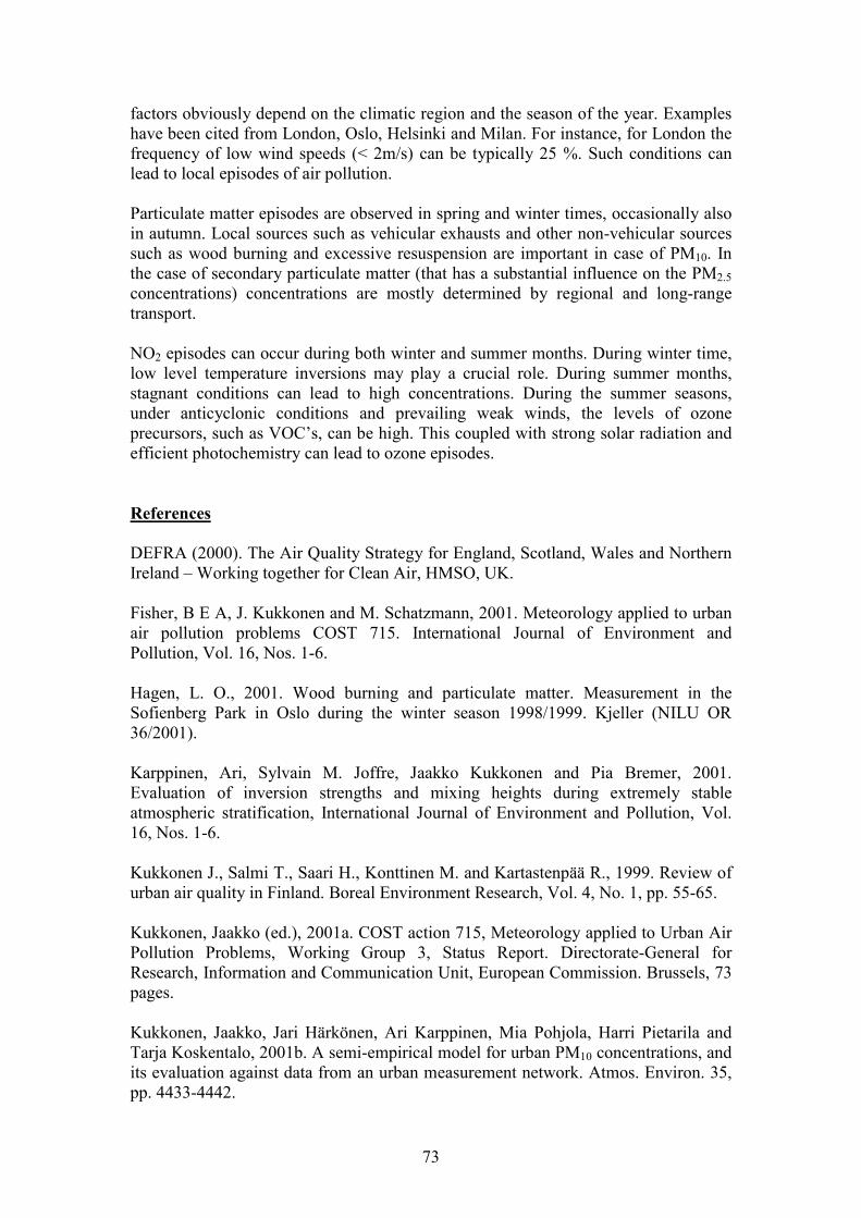
73

factors obviously depend on the climatic region and the season of the year. Exampleshave been cited from London, Oslo, Helsinki and Milan. For instance, for London thefrequency of low wind speeds (< 2m/s) can be typically 25 %. Such conditions canlead to local episodes of air pollution.

Particulate matter episodes are observed in spring and winter times, occasionally alsoin autumn. Local sources such as vehicular exhausts and other non-vehicular sourcessuch as wood burning and excessive resuspension are important in case of PM10. Inthe case of secondary particulate matter (that has a substantial influence on the PM2.5concentrations) concentrations are mostly determined by regional and long-rangetransport.

NO2 episodes can occur during both winter and summer months. During winter time,low level temperature inversions may play a crucial role. During summer months,stagnant conditions can lead to high concentrations. During the summer seasons,under anticyclonic conditions and prevailing weak winds, the levels of ozoneprecursors, such as VOC’s, can be high. This coupled with strong solar radiation andefficient photochemistry can lead to ozone episodes.

References

DEFRA (2000). The Air Quality Strategy for England, Scotland, Wales and NorthernIreland – Working together for Clean Air, HMSO, UK.

Fisher, B E A, J. Kukkonen and M. Schatzmann, 2001. Meteorology applied to urbanair pollution problems COST 715. International Journal of Environment andPollution, Vol. 16, Nos. 1-6.

Hagen, L. O., 2001. Wood burning and particulate matter. Measurement in theSofienberg Park in Oslo during the winter season 1998/1999. Kjeller (NILU OR36/2001).

Karppinen, Ari, Sylvain M. Joffre, Jaakko Kukkonen and Pia Bremer, 2001.Evaluation of inversion strengths and mixing heights during extremely stableatmospheric stratification, International Journal of Environment and Pollution, Vol.16, Nos. 1-6.

Kukkonen J., Salmi T., Saari H., Konttinen M. and Kartastenpää R., 1999. Review ofurban air quality in Finland. Boreal Environment Research, Vol. 4, No. 1, pp. 55-65.

Kukkonen, Jaakko (ed.), 2001a. COST action 715, Meteorology applied to Urban AirPollution Problems, Working Group 3, Status Report. Directorate-General forResearch, Information and Communication Unit, European Commission. Brussels, 73pages.

Kukkonen, Jaakko, Jari Härkönen, Ari Karppinen, Mia Pohjola, Harri Pietarila andTarja Koskentalo, 2001b. A semi-empirical model for urban PM10 concentrations, andits evaluation against data from an urban measurement network. Atmos. Environ. 35,pp. 4433-4442.

74

Middleton D R and Dixon J 2002. On the Recurrence of Air Pollution Episodes.Turbulence and Diffusion Note No 269, Met Office, UK.

QUARG, 1993. Urban Air Quality in the United Kingdom, First Report of the Qualityof Urban Air Review Group, Department of Environment, UK.

QUARG, 1996. Airborne Particulate Matter in the United Kingdom, Third Report ofthe Quality of Urban Air Review Group, Department of Environment, UK.

Pohjola, M A, Kousa, A, Kukkonen, J, Härkönen, J, Karppinen, A, Aarnio, P,Koskentalo, T, 2002. The Spatial and Temporal Variation of Measured Urban PM10and PM2.5 concentrations in the Helsinki Metropolitan Area. Water, Air and SoilPollution: Focus (in print).

Slørdal, L. H. and S. Larssen, 2001. Indoor wood burning and airborne particles.Model calculations for Oslo for the winter of 1998-1999. Kjeller (NILU OR 37/2001).

75

Simulations of wintertime inversions in northern European cities by useof NWP-models.

by

Erik Berge1, Ari Karppinen2, Jaakko Kukkonen2, Morten Ø. Køltzow1 and Leiv HåvardSlørdal3.

1The Norwegian Meteorological Institute2Finnish Meteorological Institute

3The Norwegian Institute for Air Research

1 IntroductionThe aim of this paper is to present results from Numerical Weather Prediction

(NWP) modeling in northern Europe during strong wintertime inversions, and to discusshow realistic these simulations are. Air quality problems in northern Europe are oftenlinked to episodes of strong inversions, and high levels of air pollutants such as NO2 andparticulate matter (PM2.5 or PM10) often occur during the episodes. Predictions of thenear surface air concentrations are crucially dependent on the prediction ofmeteorological quantities such as wind speed and direction and the vertical temperaturedistribution.

Today’s meteorological models have become rather elaborate with respect tophysical parameterization and treatment of surface processes. Together with present highspeed computers, it is now possible to run operational NWP-models with sufficienthorizontal and vertical resolution to resolve small scale wind and temperaturedistributions linked to the wintertime episodes of high levels of pollutants. Thesimulations discussed in this paper are based on the utilization of an operational fine-scale NWP-system developed for the larger cities in Norway (see Berge et al. 2002). Inthe present paper, we have applied this NWP-system to study strong winter timeinversions in Oslo, Norway and Helsinki, Finland.

2 Model descriptionFor the Oslo study we employ the HIRLAM hydrostatic model. (HIRLAM=HIgh

Resolution Limited Area model, (see Kállén 1996)) in order to obtain large scalemeteorological fields. The model is operated on a 50 km and a 10 km grid. The 10 kmversion (henceforth denoted HIRLAM10) has 31 layers in the vertical and covers NWEurope and adjacent seas (see Fig 1). The non-hydrostatic MM5 model version 3 (FifthGeneration NCAR/Penn State University Meso-scale Modeling System, see Dudhia(1993) and Grell et al., 1994) has been nested within the HIRLAM10 model. Detailsabout the nesting of MM5 with HIRLAM10 data and an evaluation of the MM5 modelcan be found in Berge et al. (2000A and B). For the Oslo region MM5 has been set up fortwo nests with 3 km and 1 km horizontal resolution respectively as shown in Fig. 1. Theinner (1km resolution) domain covers the city plus the nearby hills and the inner part ofthe Oslo fjord. The meteorological data from this nest is further utilized for air qualitysimulations in Oslo.

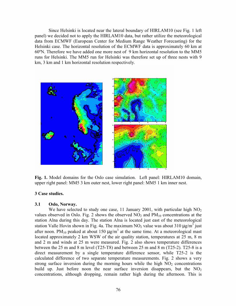
76

Since Helsinki is located near the lateral boundary of HIRLAM10 (see Fig. 1 leftpanel) we decided not to apply the HIRLAM10 data, but rather utilize the meteorologicaldata from ECMWF (European Center for Medium Range Weather Forecasting) for theHelsinki case. The horizontal resolution of the ECMWF data is approximately 60 km at60ºN. Therefore we have added one more nest of 9 km horizontal resolution to the MM5runs for Helsinki. The MM5 run for Helsinki was therefore set up of three nests with 9km, 3 km and 1 km horizontal resolution respectively.

Fig. 1. Model domains for the Oslo case simulation. Left panel: HIRLAM10 domain,upper right panel: MM5 3 km outer nest, lower right panel: MM5 1 km inner nest.

3 Case studies.

3.1 Oslo, Norway.We have selected to study one case, 11 January 2001, with particular high NO2

values observed in Oslo. Fig. 2 shows the observed NO2 and PM10 concentrations at thestation Alna during this day. The station Alna is located just east of the meteorologicalstation Valle Hovin shown in Fig. 4a. The maximum NO2 value was about 310 µg/m3 justafter noon. PM10 peaked at about 150 µg/m3 at the same time. At a meteorological mastlocated approximately 2 km WSW of the air quality station, temperatures at 25 m, 8 mand 2 m and winds at 25 m were measured. Fig. 2 also shows temperature differencesbetween the 25 m and 8 m level (T25-T8) and between 25 m and 8 m (T25-2). T25-8 is adirect measurement by a single temperature difference sensor, while T25-2 is thecalculated difference of two separate temperature measurements. Fig. 2 shows a verystrong surface inversion during the morning hours while the high NO2 concentrationsbuild up. Just before noon the near surface inversion disappears, but the NO2concentrations, although dropping, remain rather high during the afternoon. This is

77

probably due to the low wind speeds persisting throughout the afternoon (see Fig. 3) andthe fact that a larger scale inversion up to a few hundred meters remains above the nearneutrally mixed layer close to the ground.

Fig. 3 present the model simulations of MM5 and HIRLAM10 compared with themeasurements. Firstly, we find a strong inversion at Valle Hovin in the MM5 T25-8 data(Fig. 2) (see Fig. 4a for the location of Valle Hovin). But, the near surface inversion is notbroken up around noon as we find from the observations. The temperature panel of Fig. 3shows rapid increase of the observed temperature after 10:00 from about -5°C to about0°C, which is probably linked to the break up of the near surface inversion. Acorresponding temperature increase is not encountered in the model simulations. MM5has a realistic temperature curve until 10:00, after this time it remains too cold.HIRLAM10 is somewhat colder than MM5 during the whole day. The underestimatedtemperature probably causes the discrepancy in the predictions of relative humidity fromnoon and the following hours.

Air concentrations at Alna-Oslo 11 January 2001

050

100150200250300350

1 3 5 7 9 11 13 15 17 19 21 23Hour

ug/m

3 NO2PM10

Inversion strength 11 January 2001

-0,500,000,501,001,502,002,503,003,50

00:00 04:00 08:00 12:00 16:00 20:00

Hour

Deg.

Cel

cius T25-T2

T25-T8MM5

Fig. 2. NO2 and PM10 concentrations (upper panel) at Alna station, Oslo, and inversionstrength measured and calculated by MM5 at Valle Hovin during 11.01.2001.

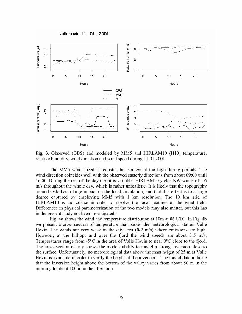
78

Fig. 3. Observed (OBS) and modeled by MM5 and HIRLAM10 (H10) temperature,relative humidity, wind direction and wind speed during 11.01.2001.

The MM5 wind speed is realistic, but somewhat too high during periods. Thewind direction coincides well with the observed easterly directions from about 09:00 until16:00. During the rest of the day the fit is variable. HIRLAM10 yields NW winds of 4-6m/s throughout the whole day, which is rather unrealistic. It is likely that the topographyaround Oslo has a large impact on the local circulation, and that this effect is to a largedegree captured by employing MM5 with 1 km resolution. The 10 km grid ofHIRLAM10 is too coarse in order to resolve the local features of the wind field.Differences in physical parameterization of the two models may also matter, but this hasin the present study not been investigated.

Fig. 4a shows the wind and temperature distribution at 10m at 06 UTC. In Fig. 4bwe present a cross-section of temperature that passes the meteorological station ValleHovin. The winds are very weak in the city area (0-2 m/s) where emissions are high.However, at the hilltops and over the fjord the wind speeds are about 3-5 m/s.Temperatures range from -5°C in the area of Valle Hovin to near 0°C close to the fjord.The cross-section clearly shows the models ability to model a strong inversion close tothe surface. Unfortunately, no meteorological data above the mast height of 25 m at ValleHovin is available in order to verify the height of the inversion. The model data indicatethat the inversion height above the bottom of the valley varies from about 50 m in themorning to about 100 m in the afternoon.

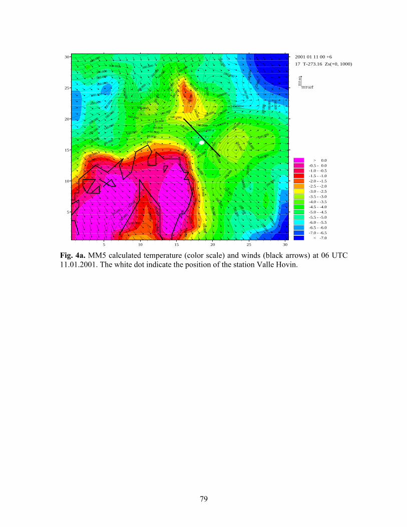
79

< -7.0-7.0 - -6.5-6.5 - -6.0-6.0 - -5.5-5.5 - -5.0-5.0 - -4.5-4.5 - -4.0-4.0 - -3.5-3.5 - -3.0-3.0 - -2.5-2.5 - -2.0-2.0 - -1.5-1.5 - -1.0-1.0 - -0.5-0.5 - 0.0

> 0.0

10.0 m/s

10.0

m/s

5 10 15 20 25 30

5

10

15

20

25

30 2001 01 11 00 +6

17 T-273.16 Zs(+0, 1000)

20.000

20.000

20.000

20.0

00

40.000

40.000

40.0

00

40.0

00

40.0

00

60.000

60.000

60.00060.000

80.000

80.000

80.0

0080

.000

100.000

100.000

100.000

100.000

120.000

120.000

120.000

120.000

120.000

140.000

140.000

140.000

140.

000

140.000

140.000

160.000

160.000

160.00016

0.000

160.000

180.000180.000

180.

000

180.000

180.000

200.000

200.

000

200.

000

220.

000

220.000

220.000

220.

000

240.000

240.000

240.000

240.

000

260.000

260.0

00

260.000

260.000

260.000

280.000

280.000

300.000

300.000

300.000

320.000

320.

000

340.000

340.0

00

360.000

360.0

00

380.000

400.000

20.000

20.000

60.00

0

60.000

40.00

0

40.000

80.000

380.000

300.000

300.000

200.000

200.0

00

200.000220.000

220.000

220.000

240.000

240.000

240.000

260.000

260.000

260.

000

180.

000

160.000

Fig. 4a. MM5 calculated temperature (color scale) and winds (black arrows) at 06 UTC11.01.2001. The white dot indicate the position of the station Valle Hovin.

80

< -4.5-4.5 - -4.0-4.0 - -3.5-3.5 - -3.0-3.0 - -2.5-2.5 - -2.0-2.0 - -1.5-1.5 - -1.0

> -1.0

20 19 18 17 16 15 140

128

255

383

5102001 01 11 00 +6

Temp. from MM5

Fig. 4b. Cross-section of temperature at 06 UTC 11.01.2001. The black line in Fig. 4ashow the position of the cross-section.

3.2 Helsinki, Finland.In the next study we focus on a simulation of the local meteorological conditions

in the Helsinki area during a severe inversion and air pollution episode by the end of1995.

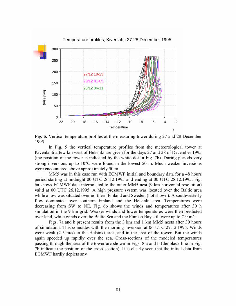
81

Fig. 5. Vertical temperature profiles at the measuring tower during 27 and 28 December1995

In Fig. 5 the vertical temperature profiles from the meteorological tower atKivenlahti a few km west of Helsinki are given for the days 27 and 28 of December 1995(the position of the tower is indicated by the white dot in Fig. 7b). During periods verystrong inversions up to 10°C were found in the lowest 50 m. Much weaker inversionswere encountered above approximately 50 m.

MM5 was in this case run with ECMWF initial and boundary data for a 48 hoursperiod starting at midnight 00 UTC 26.12.1995 and ending at 00 UTC 28.12.1995. Fig.6a shows ECMWF data interpolated to the outer MM5 nest (9 km horizontal resolution)valid at 00 UTC 26.12.1995. A high pressure system was located over the Baltic areawhile a low was situated over northern Finland and Sweden (not shown). A southwesterlyflow dominated over southern Finland and the Helsinki area. Temperatures weredecreasing from SW to NE. Fig. 6b shows the winds and temperatures after 30 hsimulation in the 9 km grid. Weaker winds and lower temperatures were then predictedover land, while winds over the Baltic Sea and the Finnish Bay still were up to 7-9 m/s.

Figs. 7a and b present results from the 3 km and 1 km MM5 nests after 30 hoursof simulation. This coincides with the morning inversion at 06 UTC 27.12.1995. Windswere weak (2-3 m/s) in the Helsinki area, and in the area of the tower. But the windsagain speeded up rapidly over the sea. Cross-sections of the modeled temperaturespassing through the area of the tower are shown in Figs. 8 a and b (the black line in Fig.7b indicate the position of the cross-section). It is clearly seen that the initial data fromECMWF hardly depicts any

5

Temperature profiles, Kivenlahti 27-28 December 1995

Temperature-22 -20 -18 -16 -14 -12 -10 -8 -6 -4 -2

height (m)

0

50

100

150

200

250

300

27/12 18-23

28/12 01-05

28/12 06-11

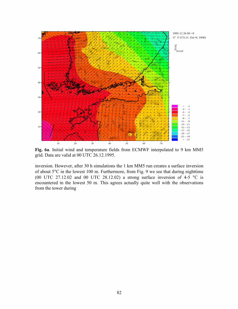
82

< -21-21 - -19-19 - -17-17 - -15-15 - -13-13 - -11-11 - -9

-9 - -7-7 - -5-5 - -3-3 - -1> -1

10.0 m/s

10.0

m/s

10 20 30 40 50 60 70

10

20

30

40

50

60

70

1995 12 26 00 +0

17 T-273.15 Zs(+0, 1000)

10.00

10.00

10.00

10.00

20.0

020

.00

20.00

20.0030.00 30.00

40.00

40.00

50.00

50.00

50.00

60.00

60.00

60.00

60.00

70.0

0

70.0

0

70.00

70.00

80.00

80.00

80.00

80.00

90.00

90.00

90.00

90.0090.00

90.00

100.00

100.00

100.

00

110.00

110.00

110.00120.00

120.0

0

120.00

120.00

130.00

140.

00

140.00

140.00

150.00

120.00

20.00

20.00

20.0

0

160.00

30.00

30.0

040.00

40.00

170.00

50.0

0

50.00

50.00

60.00

60.00

70.00

70.00

70.00

70.0

0

90.00

80.0050.00

90.0

0

130.00

120.00

110.

00

30.00

120.

00

60.00

80.00

90.00

60.00

30.00

70.00

70.00

80.00

60.00

50.00

120.00

80.0

0

130.00

70.0060.00

150.00

20.0010.00

Fig. 6a. Initial wind and temperature fields from ECMWF interpolated to 9 km MM5grid. Data are valid at 00 UTC 26.12.1995.

inversion. However, after 30 h simulations the 1 km MM5 run creates a surface inversionof about 5°C in the lowest 100 m. Furthermore, from Fig. 9 we see that during nighttime(00 UTC 27.12.02 and 00 UTC 28.12.02) a strong surface inversion of 4-5 °C isencountered in the lowest 50 m. This agrees actually quite well with the observationsfrom the tower during

83

< -21-21 - -19-19 - -17-17 - -15-15 - -13-13 - -11-11 - -9

-9 - -7-7 - -5-5 - -3-3 - -1> -1

10.0 m/s

10.0

m/s

10 20 30 40 50 60 70

10

20

30

40

50

60

70

1995 12 26 00 +30

17 T-273.15 Zs(+0, 1000)

10.00

10.00

10.00

10.00

20.0

020

.00

20.00

20.0030.00 30.00

40.00

40.00

50.00

50.00

50.00

60.00

60.00

60.00

60.00

70.0

0

70.0

0

70.00

70.00

80.00

80.00

80.00

80.00

90.00

90.00

90.00

90.0090.00

90.00

100.00

100.00

100.

00

110.00

110.00

110.00120.00

120.0

0

120.00

120.00

130.00

140.

00

140.00

140.00

150.00

120.00

20.00

20.00

20.0

0

160.00

30.00

30.0

040.00

40.00

170.00

50.0

0

50.00

50.00

60.00

60.00

70.00

70.00

70.00

70.0

0

90.00

80.0050.00

90.0

0

130.00

120.00

110.

00

30.00

120.

00

60.00

80.00

90.00

60.00

30.00

70.00

70.00

80.00

60.00

50.00

120.00

80.0

0

130.00

70.0060.00

150.00

20.0010.00

Fig. 6b. Wind and temperature fields from the 9 km MM5 grid after 30 hours of modelsimulations. Data are valid at 006UTC 27.12.1995.

84

< -14-14 - -13-13 - -12-12 - -11-11 - -10-10 - -9

-9 - -8-8 - -7-7 - -6-6 - -5-5 - -4-4 - -3-3 - -2> -2

10.0 m/s

10.0

m/s

10 20 30 40

10

20

30

40

1995 12 26 00 +30

17 T-273.15 Zs(+0, 1000)

10.00

10.00

10.00

10.00

10.00

20.00

20.0

0

20.00

20.00

20.0

0

30.00

30.00

30.00

30.00

30.00

30.00

40.00

40.00

40.00

40.00

40.00

40.00

50.00

50.00

50.00

50.0

0

50.00

50.00

60.00

60.00

60.0

0

60.00

60.00

60.00

60.0

0

60.00

70.00

70.0

0

70.00

70.00

70.00

70.00

70.00

80.00

80.0

080

.00

80.00

80.00

80.00

90.00 90.00

90.0

0

90.00

100.00

100.00

100.

00

100.00

110.00

110.

00

110.00

110.

00

110.00120.

00120.00

120.00

120.00

120.00

130.

00

130.00

Fig. 7a. Wind and temperature fields from the 3 km MM5 grid after 30 hours of modelsimulations. Data are valid at 06 UTC 27.12.1995.

the evening 27.12.02 although the observations show an even stronger inversion and 2-4 °C lowertemperatures near the surface. (Fig. 5). As already mentioned, the observations indicate aninversion top at about 50 m. We therefore find that the structure of the inversion is realisticallysimulated although the magnitude is somewhat underestimated.

85

< -11.0-11.0 - -10.0-10.0 - -9.0

-9.0 - -8.0-8.0 - -7.0-7.0 - -6.0-6.0 - -5.0-5.0 - -4.0-4.0 - -3.0

> -3.0

10.0 m/s

10.0

m/s

10 20 30 40

10

20

30

40

1995 12 26 00 +30

17 T-273.16 Zs(+0, 1000)

20.0

000

20.0000

20.0000

20.0

000

20.00

00

20.00

00

30.0000

30.0000

30.0000

30.0000

30.0000

30.0

000

30.0000

40.0000

40.0000

40.0000

40.0000

40.0000

40.0000

40.0000

50.0000

50.0000

50.0000

50.0000

50.0

000

50.0000

50.0

000

60.0000

60.0000

60.00

00

60.0000

60.0

000

70.0000

70.000070

.000

0

70.0000

80.0000

80.0000

80.0

000

10.00

00

10.00

00

10.0000

10.0000

10.0000

90.0000

90.0000

60.0000

Fig. 7b. Wind and temperature fields from the 1 km MM5 grid after 30 hours of modelsimulations. Data are valid at 06 UTC 27.12.1995.

< -10.00-10.00 - -9.60

-9.60 - -9.20-9.20 - -8.80-8.80 - -8.40-8.40 - -8.00-8.00 - -7.60-7.60 - -7.20-7.20 - -6.80-6.80 - -6.40-6.40 - -6.00

> -6.00

5 10 15 20 250

200

400

600

1995 12 26 00 +0

T-273.15

Fig. 8a. Cross-section of temperature at 00 UTC 26.12.1995. The black line in Fig. 7bshows the position of the cross-section.

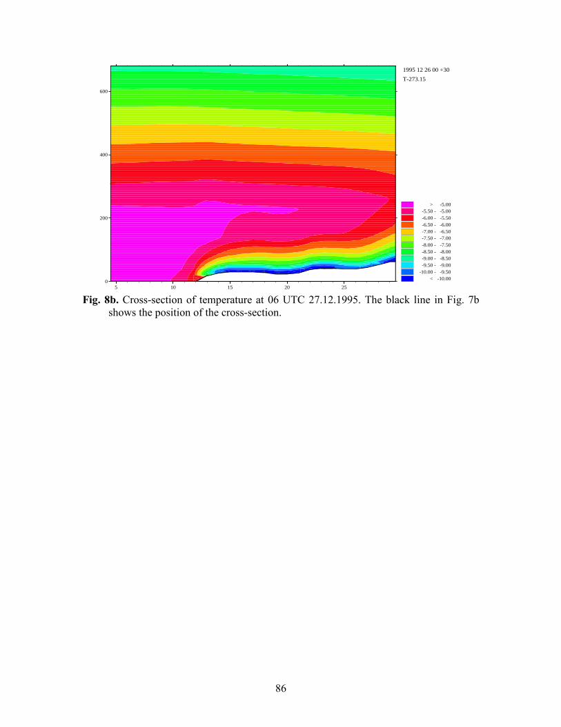
86

< -10.00-10.00 - -9.50

-9.50 - -9.00-9.00 - -8.50-8.50 - -8.00-8.00 - -7.50-7.50 - -7.00-7.00 - -6.50-6.50 - -6.00-6.00 - -5.50-5.50 - -5.00

> -5.00

5 10 15 20 250

200

400

600

1995 12 26 00 +30

T-273.15

Fig. 8b. Cross-section of temperature at 06 UTC 27.12.1995. The black line in Fig. 7bshows the position of the cross-section.

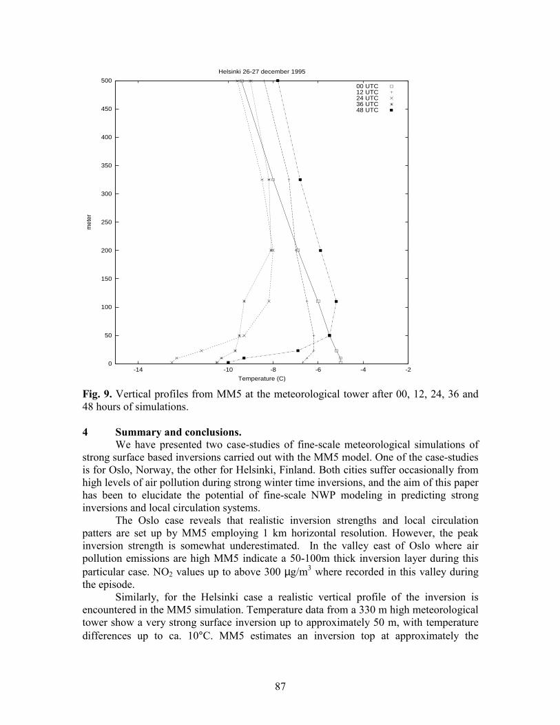
87

0

50

100

150

200

250

300

350

400

450

500

-14 -10 -8 -6 -4 -2

met

er

Temperature (C)

Helsinki 26-27 december 1995

00 UTC12 UTC24 UTC36 UTC48 UTC

Fig. 9. Vertical profiles from MM5 at the meteorological tower after 00, 12, 24, 36 and48 hours of simulations.

4 Summary and conclusions.We have presented two case-studies of fine-scale meteorological simulations of

strong surface based inversions carried out with the MM5 model. One of the case-studiesis for Oslo, Norway, the other for Helsinki, Finland. Both cities suffer occasionally fromhigh levels of air pollution during strong winter time inversions, and the aim of this paperhas been to elucidate the potential of fine-scale NWP modeling in predicting stronginversions and local circulation systems.

The Oslo case reveals that realistic inversion strengths and local circulationpatters are set up by MM5 employing 1 km horizontal resolution. However, the peakinversion strength is somewhat underestimated. In the valley east of Oslo where airpollution emissions are high MM5 indicate a 50-100m thick inversion layer during thisparticular case. NO2 values up to above 300 µg/m3 where recorded in this valley duringthe episode.

Similarly, for the Helsinki case a realistic vertical profile of the inversion isencountered in the MM5 simulation. Temperature data from a 330 m high meteorologicaltower show a very strong surface inversion up to approximately 50 m, with temperaturedifferences up to ca. 10°C. MM5 estimates an inversion top at approximately the

88

measured level, however the inversion strength is typically 2-4 °C smaller than themeasured values. No wind data comparison has been conducted for the Helsinki case.

It is recommended for the future to employ sensitivity studies in order tounderstand the reasons for the underestimations of the inversion strength. One mayspeculate why the model is not able to build up low enough surface temperatures. Oneexplanation could be insufficient surface data on snow and ice coverage and groundtemperatures. For the Helsinki case it is also recommended as a next step to comparemodeled and measured wind profiles. The measuring tower is situated well away fromthe urban areas of Helsinki thus the measurements should not be influenced by urbaneffects. In Oslo however, urban effects may play an important role and develop an urbanboundary layer (UBL), and hence it is also recommended to test UBL parameterizationsin MM5.

5 References

Berge, E., Walker, S-E., Sorteberg, A., Lenkopane, M., Eastwood, S., Jablonska, H.J. ogØdegaard. M. 2002. A real-time forecast model for meteorology and air quality during peakair pollution episodes in Oslo, Norway. Water Air and Soil Pollution. Special Issue: UrbanAir Quality – Recent Advances. In press.

Berge, E, Walker, S-E., Sorteberg, A, Eastwood, S., Kristiansen, J og Tønnesen, D. 2000A.Utvikling og testing av pilotmodell for luftkvaliteten i Oslo. Research Report no. 99, TheNorwegian Meteororlogical Institute, Oslo, Norway.

Berge, E., Walker, S-E., Sorteberg, A., Lenkopane, M., Eastwood, S., Jablonska, H.J. ogØdegaard. M. 2000B. Evaluering av prognosemodell for meteorologi og luftkvalitet for 22vinterdager i Oslo. Research Report no. 100. The Norwegian Meteorological Institute. Oslo.Norway.

Dudhia, J. 1993. A nonhydrostatic version of the Penn State/NCAR mesoscale model: Validationtests and simulation of an Atlantic cyclone and cold front. Mon. Wea. Rev., 121, 1493-1513.

Grell, G.A., Dudhia, J. and Stauffer, D.R. 1994. A description of the fifth-generation PennState/NCAR mesoscale model (MM5). NCAR Technical Note, NCAR/TN-397+IA, 114p.

Källén, E. 1996. Hirlam documentation manual system 2.5. Available at the NorwegianMeteorological Institute, Oslo, Norway.

89

Evaluation of meteorological data measured at a radio towerin the Helsinki Metropolitan Area

Ari Karppinen, Sylvain M. Joffre and Jaakko Kukkonen

Finnish Meteorological Institute,Sahaajankatu 20 E, 00880 HELSINKI, FINLAND

Abstract

We have evaluated the meteorological data measured at a radio tower of 327 m height,called the Kivenlahti mast, situated in the Helsinki Metropolitan Area. Measurementinstruments have been located at nine levels from 5 m to 327 m. The archived datacontains wind speed and direction, ambient temperature and relative humidity values,averaged within 10 minutes, as well as one-minute minimum and maximum values forwind speed and direction, since 1989. We have analyzed the wind speed and directiondata from the mast during a period of ten years, from 1989 to 1998. The roughness length(z0) in the vicinity of the mast varies from approximately 1.5 m to 3.0 m. The z0 valuesare lowest in the South-Western wind direction sector, caused by the surrounding seaareas; as expected, the maximum z0 value is observed approximately in the direction ofthe nearest city centre (Espoo). The analysis performed at the height level of 27 m alsoshowed that the wind speed values are disturbed by the presence of the mast itself. Such adisturbance takes place in a specific wind direction sector, in which the instruments are inthe lee side of the structure, approximately from 20° to 80°. The dataset is available forstudies addressing the structure of urban atmospheres. The data has been utilisedespecially in evaluating the temporal evolution of temperature inversions in the course ofpeak pollution episodes.

1. Introduction

Urban areas influence atmospheric flow both mechanically and thermally. Urbanroughness elements are commonly heterogeneously distributed; it is therefore difficult todefine a specific reference surface regarding wind speed and direction. The classicalsimilarity theories of the surface layer are not generally valid. The vertical surfaces ofbuildings contribute to an atmospheric energy exchange that is substantially different,compared with that in the surrounding rural environment (e.g., Fisher et al., 2001).

Routine meteorological observations are commonly mostly conducted in rural areas. It istherefore especially important to analyse the meteorological data that has been measuredin urban areas. It is also useful to compare such observations with the correspondingvalues measured in rural areas. Measured data is especially scarce concerning the verticalstructure of the boundary layer in urban environments.

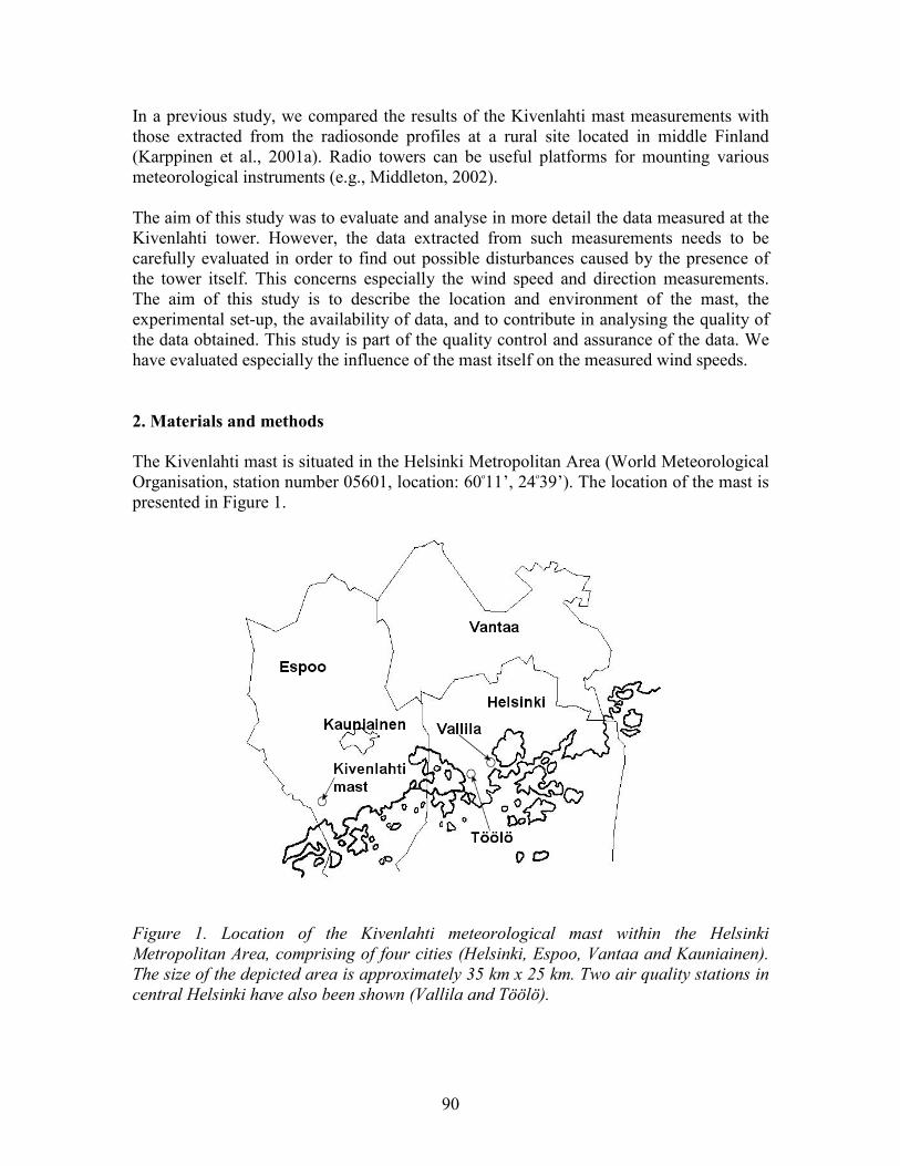
90

In a previous study, we compared the results of the Kivenlahti mast measurements withthose extracted from the radiosonde profiles at a rural site located in middle Finland(Karppinen et al., 2001a). Radio towers can be useful platforms for mounting variousmeteorological instruments (e.g., Middleton, 2002).

The aim of this study was to evaluate and analyse in more detail the data measured at theKivenlahti tower. However, the data extracted from such measurements needs to becarefully evaluated in order to find out possible disturbances caused by the presence ofthe tower itself. This concerns especially the wind speed and direction measurements.The aim of this study is to describe the location and environment of the mast, theexperimental set-up, the availability of data, and to contribute in analysing the quality ofthe data obtained. This study is part of the quality control and assurance of the data. Wehave evaluated especially the influence of the mast itself on the measured wind speeds.

2. Materials and methods

The Kivenlahti mast is situated in the Helsinki Metropolitan Area (World MeteorologicalOrganisation, station number 05601, location: 60o11’, 24o39’). The location of the mast ispresented in Figure 1.

Figure 1. Location of the Kivenlahti meteorological mast within the HelsinkiMetropolitan Area, comprising of four cities (Helsinki, Espoo, Vantaa and Kauniainen).The size of the depicted area is approximately 35 km x 25 km. Two air quality stations incentral Helsinki have also been shown (Vallila and Töölö).

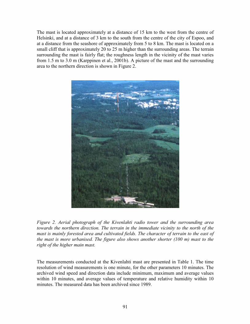
91

The mast is located approximately at a distance of 15 km to the west from the centre ofHelsinki, and at a distance of 3 km to the south from the centre of the city of Espoo, andat a distance from the seashore of approximately from 5 to 8 km. The mast is located on asmall cliff that is approximately 20 to 25 m higher than the surrounding areas. The terrainsurrounding the mast is fairly flat; the roughness length in the vicinity of the mast variesfrom 1.5 m to 3.0 m (Karppinen et al., 2001b). A picture of the mast and the surroundingarea to the northern direction is shown in Figure 2.

Figure 2. Aerial photograph of the Kivenlahti radio tower and the surrounding areatowards the northern direction. The terrain in the immediate vicinity to the north of themast is mainly forested area and cultivated fields. The character of terrain to the east ofthe mast is more urbanised. The figure also shows another shorter (100 m) mast to theright of the higher main mast.

The measurements conducted at the Kivenlahti mast are presented in Table 1. The timeresolution of wind measurements is one minute, for the other parameters 10 minutes. Thearchived wind speed and direction data include minimum, maximum and average valueswithin 10 minutes, and average values of temperature and relative humidity within 10minutes. The measured data has been archived since 1989.

92

Table 1. The meteorological measurements conducted at the Kivenlahti mast.

Meteorologicalparameter

Measurement height (m)

5 26 48 91 142 182 266 296 327Wind speed x x x xWind direction x x x xTemperature x x x x x x X xRelative humidity x x x x

A more detailed picture of the wind sensors at one specific height is presented in Figure3. Wind sensors (Hydrotech WS-3) are located on the South-Western side of the mast. Ateach measurement level, sensors are situated on a boom that extends from the maststructure to reduce its disturbing effects.

Figure 3. The wind sensors at the height of 26 m in the Kivenlahti mast (on the left-hand-side of the mast). The photograph has been taken from the southern direction.

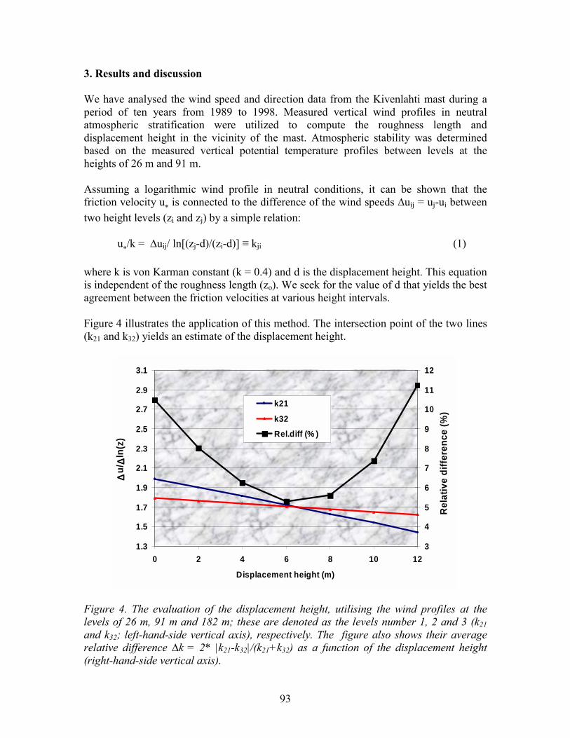
93

3. Results and discussion

We have analysed the wind speed and direction data from the Kivenlahti mast during aperiod of ten years from 1989 to 1998. Measured vertical wind profiles in neutralatmospheric stratification were utilized to compute the roughness length anddisplacement height in the vicinity of the mast. Atmospheric stability was determinedbased on the measured vertical potential temperature profiles between levels at theheights of 26 m and 91 m.

Assuming a logarithmic wind profile in neutral conditions, it can be shown that thefriction velocity u* is connected to the difference of the wind speeds ∆uij = uj-ui betweentwo height levels (zi and zj) by a simple relation:

u*/k = ∆uij/ ln[(zj-d)/(zi-d)] ≡ kji (1)

where k is von Karman constant (k = 0.4) and d is the displacement height. This equationis independent of the roughness length (zo). We seek for the value of d that yields the bestagreement between the friction velocities at various height intervals.

Figure 4 illustrates the application of this method. The intersection point of the two lines(k21 and k32) yields an estimate of the displacement height.

1.3

1.5

1.7

1.9

2.1

2.3

2.5

2.7

2.9

3.1

0 2 4 6 8 10 12

Displacement height (m)

∆∆ ∆∆u/∆∆ ∆∆

ln(z

)

3

4

5

6

7

8

9

10

11

12

Rel

ativ

e di

ffere

nce

(%)

k21

k32Rel.diff (% )

Figure 4. The evaluation of the displacement height, utilising the wind profiles at thelevels of 26 m, 91 m and 182 m; these are denoted as the levels number 1, 2 and 3 (k21and k32; left-hand-side vertical axis), respectively. The figure also shows their averagerelative difference ∆k = 2* |k21-k32|/(k21+k32) as a function of the displacement height(right-hand-side vertical axis).

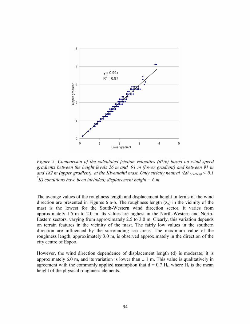
94

y = 0.99x R2 = 0.97

0

1

2

3

4

5

0 1 2 3 4 5Lower gradient

Upp

er g

radi

ent

Figure 5. Comparison of the calculated friction velocities (u*/k) based on wind speedgradients between the height levels 26 m and 91 m (lower gradient) and between 91 mand 182 m (upper gradient), at the Kivenlahti mast. Only strictly neutral (∆θ (29-91m) < 0.1oK) conditions have been included; displacement height = 6 m.

The average values of the roughness length and displacement height in terms of the winddirection are presented in Figures 6 a-b. The roughness length (zo) in the vicinity of themast is the lowest for the South-Western wind direction sector, it varies fromapproximately 1.5 m to 2.0 m. Its values are highest in the North-Western and North-Eastern sectors, varying from approximately 2.5 to 3.0 m. Clearly, this variation dependson terrain features in the vicinity of the mast. The fairly low values in the southerndirection are influenced by the surrounding sea areas. The maximum value of theroughness length, approximately 3.0 m, is observed approximately in the direction of thecity centre of Espoo.

However, the wind direction dependence of displacement length (d) is moderate; it isapproximately 6.0 m, and its variation is lower than ± 1 m. This value is qualitatively inagreement with the commonly applied assumption that d = 0.7 Hr, where Hr is the meanheight of the physical roughness elements.

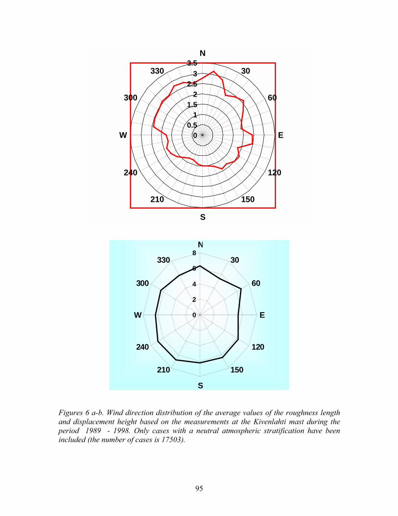
95

00.5

11.5

22.5

33.5

N

30

60

E

120

150

S

210

240

W

300

330

0

2

4

6

8N

30

60

E

120

150

S

210

240

W

300

330

Figures 6 a-b. Wind direction distribution of the average values of the roughness lengthand displacement height based on the measurements at the Kivenlahti mast during theperiod 1989 - 1998. Only cases with a neutral atmospheric stratification have beenincluded (the number of cases is 17503).

96

The averaged wind speed values in terms of the wind direction are presented in Figures 7a-b at two specific measurement levels. Clearly, the wind speed values are dependent onthe synoptic weather conditions and the origin of the air masses. For instance, synopticweather systems that have been transported from the Northernmost parts of the Atlanticor from the Northernmost parts of Russia can more commonly cause a prevailing stableatmospheric stratification, with associated weak wind speeds. We have therefore includedonly one stability regime (unstable cases) in the present analysis.

012345678

0

30

60

90

120

150

180

210

240

270

300

330

Isosaari 84-90Katajaluoto 71-84Hki-Vantaa 71-86Kivenlahti 92m 75-80

Figures 7 a-b. (a) The average values of the wind speed in terms of the wind direction,based on the measurements at the Kivenlahti mast (unstable stratification) during theperiod from 1989 to 1998 at the height of 26 meters. (b) The average values of the windspeed in terms of the wind direction, based on the measurements at 3 synoptic stations inthe vicinity of the Helsinki area during 1971 - 1990, and the Kivenlahti mast during theperiod from 1975 to 1980 at the height of 92 meters (Tammelin, 1991).

Figure 7b shows examples of the synoptic-scale influence on the wind speeds in terms ofwind direction. Comparison of the data determined at various stations shows that thewind direction dependence of the wind speeds at the station of Kivenlahti is clearlyinfluenced by the presence of the mast itself, and by other equipment and structuresattached to the mast.

The results in Figures 7 a-b show a decreased wind speed in the wind direction sectorapproximately from 20 to 80°. This decrease is caused by the disturbances caused by themast and other structures attached to it, in the lee side of the structure. We thereforerecommend that the data corresponding to this wind direction interval should be removedfrom any analysis that addresses wind velocities, or other parameters related to the windvelocity.

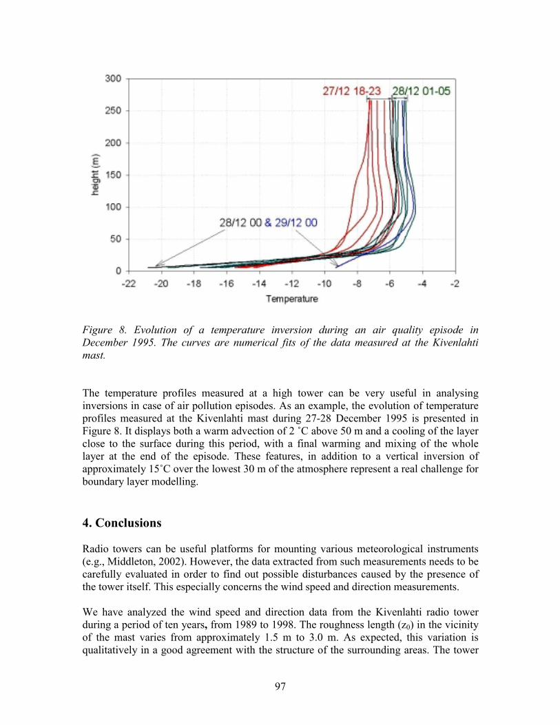
97

Figure 8. Evolution of a temperature inversion during an air quality episode inDecember 1995. The curves are numerical fits of the data measured at the Kivenlahtimast.

The temperature profiles measured at a high tower can be very useful in analysinginversions in case of air pollution episodes. As an example, the evolution of temperatureprofiles measured at the Kivenlahti mast during 27-28 December 1995 is presented inFigure 8. It displays both a warm advection of 2 ˚C above 50 m and a cooling of the layerclose to the surface during this period, with a final warming and mixing of the wholelayer at the end of the episode. These features, in addition to a vertical inversion ofapproximately 15˚C over the lowest 30 m of the atmosphere represent a real challenge forboundary layer modelling.

4. Conclusions

Radio towers can be useful platforms for mounting various meteorological instruments(e.g., Middleton, 2002). However, the data extracted from such measurements needs to becarefully evaluated in order to find out possible disturbances caused by the presence ofthe tower itself. This especially concerns the wind speed and direction measurements.

We have analyzed the wind speed and direction data from the Kivenlahti radio towerduring a period of ten years, from 1989 to 1998. The roughness length (z0) in the vicinityof the mast varies from approximately 1.5 m to 3.0 m. As expected, this variation isqualitatively in a good agreement with the structure of the surrounding areas. The tower

98

is located within the Helsinki Metropolitan Area; however, it is in the westernmost part ofthe area that is not in the immediate vicinity of the major buildings in central Helsinki.

The analysis for unstable cases at the measurement level of 26 and 92 m has shown thatthe wind speed measurements can be disturbed by the presence of the mast itself, and theattached instruments and equipment. This disturbance is evident in one specific winddirection sector, approximately from 20° to 80°; for this specific sector, the anemometersare in the lee side of the structure. We recommend that the data corresponding to thiswind direction sector should be removed from any analysis that addresses wind velocitiesor other parameters related to the wind velocity. In future work, the correspondinganalysis could be performed systematically for all stability regimes and measurementlevels.

The temperature profiles measured at such a tower can be very useful in analysinginversions in case of air pollution episodes. The dataset is available for studies addressingthe structure of urban atmospheres.

5. References

Fisher, B E A, J. Kukkonen and M. Schatzmann, 2001. Meteorology applied to urban airpollution problems COST 715. International J. Environ. and Poll., 16, 1-6.

Karppinen, A, J. Kukkonen, T. Elolähde, M. Konttinen, T. Koskentalo and E.Rantakrans, 2000a. A modelling system for predicting urban air pollution, Modeldescription and applications in the Helsinki metropolitan area. Atmos. Environ. 34 (22),3723-3733.

Karppinen, A, Kukkonen, J., Elolähde, T.,Konttinen, M. and Koskentalo, T., 2000b: Amodelling system for predicting urban air pollution, Comparison of model predictionswith the data of an urban measurement network. Atmos. Environ. 34, 3735-3743.

Karppinen, Ari, Sylvain M. Joffre, Jaakko Kukkonen and Pia Bremer, 2001a. Evaluationof inversion strengths and mixing heights during extremely stable atmosphericstratification. International J. Environ. and Poll., 16 ( 1-6).

Karppinen, A., S. M. Joffre and J. Kukkonen, 2001b. The refinement of a meteorologicalpreprocessor for the urban environment. International J. of Environ. and Poll., 14 (1-6),565-572.

Middleton, D.R., 2002. Meteorological challenges in urban air pollution. Clean Air 32,14-19.

Tammelin, B., 1991. Finnish Wind Atlas,. Finnish Meteorological Institute, Valtionpainatuskeskus, Helsinki, Finland. (ISBN 951-697-334-5).

99

Analysis of three air pollution episodes driven by a temperature inversionin a sub-alpine Italian region

Sandro Finardi1, Gabriele Carboni2, and Gianni Tinarelli1

1. ARIANET s.r.l., viale Elvezia 42, 20052 Monza (MI), ITALY2. ENEL S.p.A./Produzione, via N.Bixio 39, 29100 Piacenza, ITALY

Abstract

Three different episodes which occurred in northern Italy are analysed: (i) a winter inversionof synoptic origin extending to more than 1000 metres a.g.l., with shallow unstable boundarylayer developing during daytime, that caused a severe pollution episode in Milan in December1998, (ii) an elevated inversion episode observed in the Northern Mediterranean coastal areaof Savona on February 1998, and (iii) a persisting ground based inversion in the Alpine valleyof Aosta on February 1997. The phenomenology of these episodes is analysed on the basis oflocal vertical profiles from soundings, meteorological and chemical measurements performedat an air quality network, and synoptic meteorological information. We describe thecharacteristics of the atmospheric circulation during inversion periods and the behaviour ofpollutant concentrations. We also discuss briefly the relevance of modelling of inversionepisodes in connection with the application of current EU directives on air quality.

Introduction

Temperature inversions are one of the most crucial atmospheric conditions that areresponsible for very high pollution levels during wintertime. The strength and persistence ofinversions, and the characteristics of the atmospheric circulation during these conditions areaffected by different factors like geographic location, regional and local topography andfeatures of the urban area.

The general situation of air pollution in the Italian urban areas, as resumed by the elaborationof the National Environmental Protection Agency (ANPA) for 1998, shows that the long termair quality standards are generally respected for SO2 , NO2 and TSP, while a large number ofexceedances are recorded for O3 nearly everywhere it is measured (countrywide statistics forPM10 are not yet available). However, the situation is different for short term episodes. Themajor Italian urban areas experience severe pollution episodes, during which the thresholdlevels for NO2 (200 µg/m3 for the 98th percentile of the hourly averages and “warning level”for hourly averages in urban areas) and O3 (180 µg/m3 for hourly averages) are oftenexceeded, e.g. during 1997 the worst station in Milan city recorded 100 hours exceeding 200µg/m3 for NO2, and many other stations in the Province recorded more than 50 exceedances.

This is the situation characterised by the air quality standards presently defined by the Italianlegislation. This state of affairs would change quite sharply, if we would consider the airpollutant limit values introduced by the recent EU directives (EC 99/30; EC 2000/69). If thenew limit values, to be achieved in 2005 and 2010, are considered, some of the major Italianurban areas would be in a state of non-compliance. The cited EU legislation states limits onthe hourly and daily averages of pollutants (e.g. NO2 and PM10) to be exceeded only a few

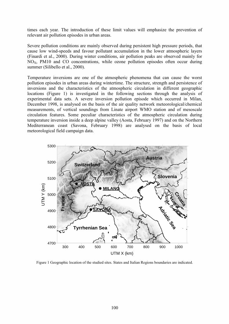
100

times each year. The introduction of these limit values will emphasize the prevention ofrelevant air pollution episodes in urban areas.

Severe pollution conditions are mainly observed during persistent high pressure periods, thatcause low wind-speeds and favour pollutant accumulation in the lower atmospheric layers(Finardi et al., 2000). During winter conditions, air pollution peaks are observed mainly forNOX, PM10 and CO concentrations, while ozone pollution episodes often occur duringsummer (Silibello et al., 2000).

Temperature inversions are one of the atmospheric phenomena that can cause the worstpollution episodes in urban areas during wintertime. The structure, strength and persistence ofinversions and the characteristics of the atmospheric circulation in different geographiclocations (Figure 1) is investigated in the following sections through the analysis ofexperimental data sets. A severe inversion pollution episode which occurred in Milan,December 1998, is analysed on the basis of the air quality network meteorological/chemicalmeasurements, of vertical soundings from Linate airport WMO station and of mesoscalecirculation features. Some peculiar characteristics of the atmospheric circulation duringtemperature inversion inside a deep alpine valley (Aosta, February 1997) and on the NorthernMediterranean coast (Savona, February 1998) are analysed on the basis of localmeteorological field campaign data.

300 400 500 600 700 800 900 1000

UTM X (km)

4700

4800

4900

5000

5100

5200

5300

UTM

Y (k

m)

SAVONA

AOSTAMILANO

SwitzerlandAustria

Slovenia

Croatia

Fran

ceAdriatic SeaTyrrhenian Sea

Figure 1 Geographic location of the studied sites. States and Italian Regions boundaries are indicated.

101

An inversion episode in Milan

Milan city and its surrounding urban area, together with several industrial settlements, islocated in the central part of the Po river basin, northern Italy, in a flat area. The whole area isexposed to substantial emission loads. The atmospheric circulation of the Po valley ischaracterised by the strong modification of synoptic flow due to the high mountains (Alps andApennines) that surround the valley on three sides. The local atmospheric circulation features,dominated by calms and weak winds, often favour the development of critical pollutionepisodes. High pollutant concentrations are generally observed during anticyclonic conditions,characterised by weak winds, high humidity and unfavourable stability conditions and limitedturbulence intensity, during winter. These conditions can be worsened by temperatureinversions which limit the vertical dilution of pollutants.

An air quality episode occurred during December 1998 that was caused by a temperatureinversion. Figure 2 shows the time evolution of NO2 and PM10 concentrations measured bythe Milan City air quality control network during December 1998.

A severe pollution episode lasting from December 14th (Monday) to December 19th

(Saturday) that can be clearly identified. The NO2 hourly average concentrations exceed boththe warning and alarm thresholds (200 and 400 µg/m3, respectively) defined for short termepisodes by the Italian law. PM10 daily averages showed values larger than 100 µg/m3 formost parts of the period. During the episode the “average” concentrations of differentpollutants show values roughly twice their monthly averages.

The observed accumulation of air pollutants is driven by an intense ground based temperatureinversion (Figure 3) that develops on December 13th and reaches its maximum depth andintensity (with a temperature growth of about 15 degrees in the first 1000 metres height) onDecember 15th and lasts until December 19th. The development of the observed inversion isdue to the advection of warm air carried by the incoming high pressure ridge, that, during theepisode, is located over the western Mediterranean basin (Fig. 4). The maximum warming isobserved between 1000 and 1500 metres a.g.l., where the temperature reaches values around15°C. Surface temperature lowers during the first days, reaching minimum vales onDecember 15th, and later starts to rise slowly. A very shallow unstable boundary layer isobserved during daytime. Its depth ranges only a few hundred meters during the wholeepisode. The local and mesoscale circulation is characterised by very low wind speeds.Surface wind observations (Figure 5) show a tendency to follow the directions of local breezecirculations.

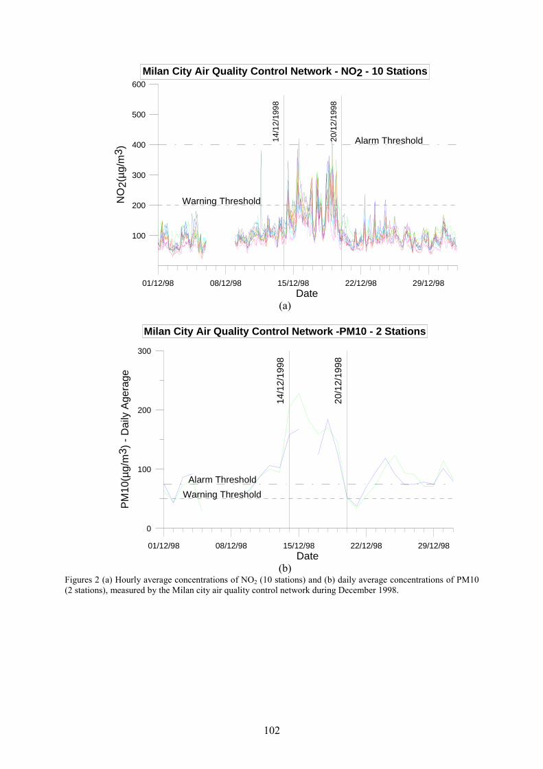
102

01/12/98 08/12/98 15/12/98 22/12/98 29/12/98Date

100

200

300

400

500

600

NO

2(µg

/m3 )

Warning Threshold

Alarm Threshold14/1

2/19

98

20/1

2/19

98

Milan City Air Quality Control Network - NO2 - 10 Stations

(a)

01/12/98 08/12/98 15/12/98 22/12/98 29/12/98Date

0

100

200

300

PM10

(µg/

m3 )

- D

aily

Age

rage

Warning ThresholdAlarm Threshold

14/1

2/19

98

20/1

2/19

98Milan City Air Quality Control Network -PM10 - 2 Stations

(b)Figures 2 (a) Hourly average concentrations of NO2 (10 stations) and (b) daily average concentrations of PM10(2 stations), measured by the Milan city air quality control network during December 1998.

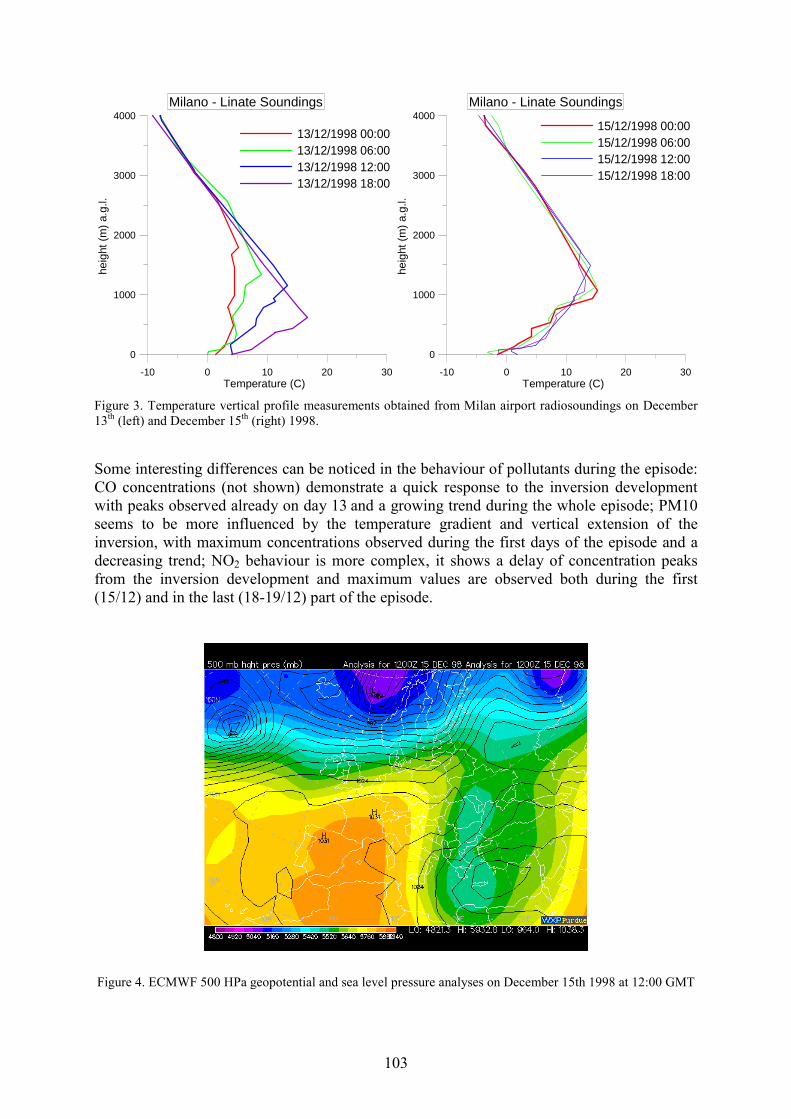
103

-10 0 10 20 30Temperature (C)

0

1000

2000

3000

4000he

ight

(m) a

.g.l.

13/12/1998 00:0013/12/1998 06:0013/12/1998 12:0013/12/1998 18:00

Milano - Linate Soundings

-10 0 10 20 30Temperature (C)

0

1000

2000

3000

4000

heig

ht (m

) a.g

.l.

15/12/1998 00:0015/12/1998 06:0015/12/1998 12:0015/12/1998 18:00

Milano - Linate Soundings

Figure 3. Temperature vertical profile measurements obtained from Milan airport radiosoundings on December13th (left) and December 15th (right) 1998.

Some interesting differences can be noticed in the behaviour of pollutants during the episode:CO concentrations (not shown) demonstrate a quick response to the inversion developmentwith peaks observed already on day 13 and a growing trend during the whole episode; PM10seems to be more influenced by the temperature gradient and vertical extension of theinversion, with maximum concentrations observed during the first days of the episode and adecreasing trend; NO2 behaviour is more complex, it shows a delay of concentration peaksfrom the inversion development and maximum values are observed both during the first(15/12) and in the last (18-19/12) part of the episode.

Figure 4. ECMWF 500 HPa geopotential and sea level pressure analyses on December 15th 1998 at 12:00 GMT

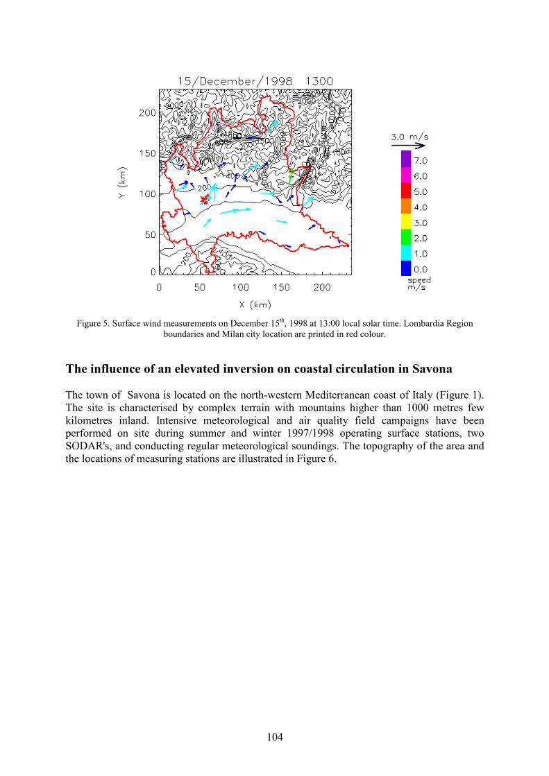
104

Figure 5. Surface wind measurements on December 15th, 1998 at 13:00 local solar time. Lombardia Regionboundaries and Milan city location are printed in red colour.

The influence of an elevated inversion on coastal circulation in Savona

The town of Savona is located on the north-western Mediterranean coast of Italy (Figure 1).The site is characterised by complex terrain with mountains higher than 1000 metres fewkilometres inland. Intensive meteorological and air quality field campaigns have beenperformed on site during summer and winter 1997/1998 operating surface stations, twoSODAR's, and conducting regular meteorological soundings. The topography of the area andthe locations of measuring stations are illustrated in Figure 6.

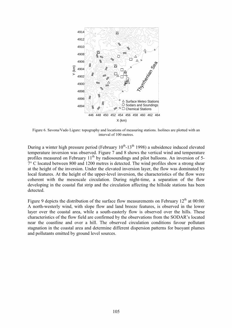
105

446 448 450 452 454 456 458 460 462 464

X (km)

4894

4896

4898

4900

4902

4904

4906

4908

4910

4912

4914

Y (k

m)

Surface Meteo Stations

Chemical StationsSodars and Soundings

Thyr

rhen

ian S

ea

Figure 6. Savona/Vado Ligure: topography and locations of measuring stations. Isolines are plotted with aninterval of 100 metres.

During a winter high pressure period (February 10th-13th 1998) a subsidence induced elevatedtemperature inversion was observed. Figure 7 and 8 shows the vertical wind and temperatureprofiles measured on February 11th by radiosoundings and pilot balloons. An inversion of 5-7° C located between 800 and 1200 metres is detected. The wind profiles show a strong shearat the height of the inversion. Under the elevated inversion layer, the flow was dominated bylocal features. At the height of the upper-level inversion, the characteristics of the flow werecoherent with the mesoscale circulation. During night-time, a separation of the flowdeveloping in the coastal flat strip and the circulation affecting the hillside stations has beendetected.

Figure 9 depicts the distribution of the surface flow measurements on February 12th at 00:00.A north-westerly wind, with slope flow and land breeze features, is observed in the lowerlayer over the coastal area, while a south-easterly flow is observed over the hills. Thesecharacteristics of the flow field are confirmed by the observations from the SODAR’s locatednear the coastline and over a hill. The observed circulation conditions favour pollutantstagnation in the coastal area and determine different dispersion patterns for buoyant plumesand pollutants emitted by ground level sources.

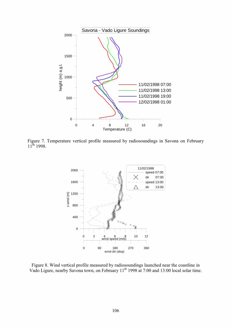
106

0 4 8 12 16 20Temperature (C)

0

500

1000

1500

2000

heig

ht (m

) a.g

.l.

11/02/1998 07:0011/02/1998 13:0011/02/1998 19:0012/02/1998 01:00

Savona - Vado Ligure Soundings

Figure 7. Temperature vertical profile measured by radiosoundings in Savona on February11th 1998.

0

400

800

1200

1600

2000

z-am

sl (m

)

0 2 4 6 8 10 12wind speed (m/s)

0 90 180 270 360wind dir (deg)

11/02/1998speed 07:00dir 07:00speed 13:00dir 13:00

Figure 8. Wind vertical profile measured by radiosoundings launched near the coastline inVado Ligure, nearby Savona town, on February 11th 1998 at 7:00 and 13:00 local solar time.

107

Figure 9 Surface wind observations on February 12th at 00:00 local solar time.

330 340 350 360 370 380 390 400 410 420

UTM32 - X (km)

5030

5040

5050

5060

5070

5080

5090

UTM

32 -

Y (k

m)

AOSTA

IVREA

Figure 10. Aosta Valley topographic features. The location of the town of Aosta, the regionalboundaries and the major roads are indicated on the map. The Mont Blanc is in the North-

western side of the map.

A persisting ground based inversion in a deep alpine valley in Aosta

Deep alpine valleys can experience persisting temperature inversions during wintertime, whenthe ground surface is generally snow-covered and the solar radiation flux is limited by theshadowing caused by topography. In these conditions air pollution episodes can affect also

108

small towns and weakly urbanised regions. Unluckily, meteorological profile measurementsare quite uncommon inside valleys, and few data are available concerning inversionconditions in southern alpine valleys.

A persisting inversion condition was observed in the Aosta Valley (Figure 1) during theperiod 30/01-07/02/1997 when a meteorological and air quality field campaign took placenearby the town of Aosta. The Aosta Valley is one of the deepest and closest valleys of theAlps (Figure 10). It faces the Mont Blanc from the Italian side, and it is surrounded on threesides by mountains reaching more than 3000 metres high, while the bottom of the valley has aheight of about 600 metres (Fig. 10). Moreover the valley axis is oriented west-east,maximising the solar shelter effects of mountains on the bottom of the valley.

The observed temperature inversion developed during a persisting high pressure conditionslowly moving over Europe. The temperature profiles measured on January 31 are plotted inFigure 11. The ground based inversion persists all day long. No unstable boundary layerdevelopment is detected by measurements. The daily air warming inside the valley simplyshifts the temperature profile without modifying its shape. The temperature inversion islimited to the first 500 metres and its strength is of the order of 5° C. The temperature profilefeatures and its daily evolution have some similarities with winter inversion conditionsobserved in Helsinki (Karppinen et al., 2002), even if the near ground temperature gradienthas lower values in the alpine valley. The observed wind profiles showed that inside theinversion layer the flow is very weak and characterised by a daily cycle with thecharacteristics of a mountain/valley breeze. The observed daily rotation is limited to the firsthour of the afternoon. The flow inside the valley appears to be separated from the circulationaloft.

-20 -10 0 10T (C)

0

1000

2000

3000

Hei

ght a

.g.l.

(m)

31/01/199701:0007:0010:0013:0016:0019:00

Aosta Soundings

Figure 11. Temperature profiles measured by radiosoundings nearby Aosta on January 31th 1997.

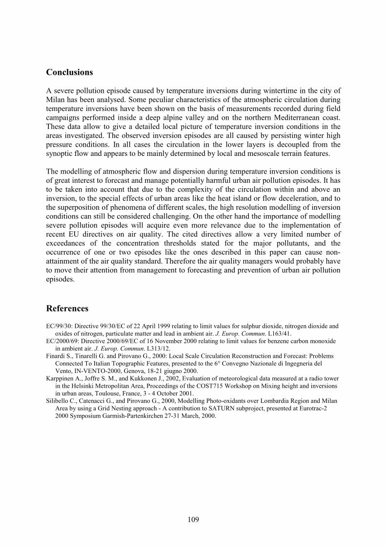
109

Conclusions

A severe pollution episode caused by temperature inversions during wintertime in the city ofMilan has been analysed. Some peculiar characteristics of the atmospheric circulation duringtemperature inversions have been shown on the basis of measurements recorded during fieldcampaigns performed inside a deep alpine valley and on the northern Mediterranean coast.These data allow to give a detailed local picture of temperature inversion conditions in theareas investigated. The observed inversion episodes are all caused by persisting winter highpressure conditions. In all cases the circulation in the lower layers is decoupled from thesynoptic flow and appears to be mainly determined by local and mesoscale terrain features.

The modelling of atmospheric flow and dispersion during temperature inversion conditions isof great interest to forecast and manage potentially harmful urban air pollution episodes. It hasto be taken into account that due to the complexity of the circulation within and above aninversion, to the special effects of urban areas like the heat island or flow deceleration, and tothe superposition of phenomena of different scales, the high resolution modelling of inversionconditions can still be considered challenging. On the other hand the importance of modellingsevere pollution episodes will acquire even more relevance due to the implementation ofrecent EU directives on air quality. The cited directives allow a very limited number ofexceedances of the concentration thresholds stated for the major pollutants, and theoccurrence of one or two episodes like the ones described in this paper can cause non-attainment of the air quality standard. Therefore the air quality managers would probably haveto move their attention from management to forecasting and prevention of urban air pollutionepisodes.

References

EC/99/30: Directive 99/30/EC of 22 April 1999 relating to limit values for sulphur dioxide, nitrogen dioxide andoxides of nitrogen, particulate matter and lead in ambient air. J. Europ. Commun. L163/41.

EC/2000/69: Directive 2000/69/EC of 16 November 2000 relating to limit values for benzene carbon monoxidein ambient air. J. Europ. Commun. L313/12.

Finardi S., Tinarelli G. and Pirovano G., 2000: Local Scale Circulation Reconstruction and Forecast: ProblemsConnected To Italian Topographic Features, presented to the 6° Convegno Nazionale di Ingegneria delVento, IN-VENTO-2000, Genova, 18-21 giugno 2000.

Karppinen A., Joffre S. M., and Kukkonen J., 2002, Evaluation of meteorological data measured at a radio towerin the Helsinki Metropolitan Area, Proceedings of the COST715 Workshop on Mixing height and inversionsin urban areas, Toulouse, France, 3 - 4 October 2001.

Silibello C., Catenacci G., and Pirovano G., 2000, Modelling Photo-oxidants over Lombardia Region and MilanArea by using a Grid Nesting approach - A contribution to SATURN subproject, presented at Eurotrac-22000 Symposium Garmish-Partenkirchen 27-31 March, 2000.

110

Conclusions and recommendationsMartin Piringer and Jaakko Kukkonen

1. General conclusions

The COST-715 - action aims at providing recommendations for harmonising the

measurements, assessments and forecasting of characteristic meteorological parameters in

the urban atmosphere. In particular, the action aims at specifying the minimum

requirements that meteorological measurements have to satisfy in urban areas.

The action also aims at a more consistent use of available urban meteorological data,

especially regarding the application of such data as input values of meteorological pre-

processors and atmospheric dispersion models. The action also supports and contributes

to new meteorological measurement campaigns in urban areas. Urban meteorological

mast data are especially valuable in order to analyse the vertical structure of the urban

canopy. In particular, atmospheric turbulence and vertical flux measurements over cities

are urgently needed. The action has already initialised some co-operative work for

utilising such data more extensively.

The action will undertake comparisons of measured urban and rural meteorological

parameters, in order to improve our understanding on urban meteorological processes.

Such a comparison is already in progress for wind speed and direction (Working Group-

WG 1); some work has also been accomplished concerning temperature inversions (WG

3).

The action needs to collaborate more closely with the World Meteorological Organisation

in the future, especially within the “Global Atmospheric Watch, Urban Research

Meteorology and Environmental Project – GURME”. For instance, the recommendations

regarding urban meteorological measurements are of common interest for both of these

actions.

111

2. Conclusions on evaluation of mixing heights

WG2 aims at a more specific definition of the mixing height (MH) for urban areas.

Useful background information has been provided by the COST-710 action; however, we

also intend to take into consideration the horizontal inhomogeneity and the vertical

structure of the boundary layer over the urban area. WG2 recommends that the MH is a

useful concept in the context of simpler regulatory dispersion models, although not a very

accurate one. Concerning numerical weather prediction (NWP) models, it is not so clear

whether the MH is sufficiently accurate to be useful.

WG2 also aims at recommending optimum methods for measuring the urban MH.

Experience has been gained based on recent field experiments, such as BUBBLE (The

Basle Urban Boundary Layer Experiment) and UBL/ESCOMPTE (The Urban Boundary

Layer Experiment in the greater Marseilles area). The effect of climatic differences on the

urban MH has to be investigated more thoroughly. There are significant differences

between, e.g., Northern and Southern European cities in this respect.

When modelling the mixing height, the mechanisms involved in the formation of the

daytime MH are better understood than the corresponding ones at nighttime. WG2

therefore strongly recommends that more emphasis should be given to improving the

methods for the nighttime MH determination.

No direct evaluation of the MH is necessary regarding the dispersion of traffic-originated

pollution within the roughness sublayer (e.g., within a street canyon). On the other hand,

in the urban and meso-scales, the MH is an important parameter for practically all air

pollution applications.

112

WG2 will also try to formulate a list of different methods for the determination of the

MH, including their relative advantages and disadvantages, and their limits of

application.

3. Conclusions on temperature inversions and peak pollution episodes

WG3 aims at a harmonised definition of an air pollution episode. WG3 also classifies

various types of air pollution episodes in Europe, in terms of the pollutants, the main

source categories and the seasons of the year. It is particularly relevant for this COST

action to investigate the evolution of various meteorological parameters in the course of

episodes. The COST 715 action will collaborate with “Formation of Ozone in South

European Cities – FOSEC” that has similar objectives specifically for Southern European

conditions. The FOSEC action is part of the SATURN project within the EUROTRAC-2

programme.

There is work in progress especially on the dependency of episodes on temperature

inversions in both Northern and Southern European countries. The action evaluates the

performance of both numerical weather prediction (NWP) models and air quality

forecasting models regarding their ability to predict relevant meteorological parameters

and air quality. A key question is the ability of such models to forecast urban temperature

inversions during episodes.

WG3 will also evaluate the dependency of episodes on the temporal variation in

emissions, and the inversions within a city compared with those in surrounding rural

areas. A set of meteorological criteria can be specified for predicting the potential

formation and occurrence of air quality episodes. Such criteria can include, e.g., limit

values in terms of wind velocity, inversion strength or gradient, atmospheric stability and

Richardson number. However, any single meteorological parameter or just one criterion

will probably not be sufficient.

113

This action should also keep in mind various policy-relevant issues, such as the

conceivable practical measures for air quality protection during episodes. It is therefore

important to inform continuously the local authorities and collaborate with them.