mike brookes - faculty of engineering · e1.10 fourier series and transforms (2014-5509) sums and...
TRANSCRIPT

E1.10 Fourier Series and Transforms (2014-5509) Sums and Averages: 1 – 1 / 14
E1.10 Fourier Series and Transforms
Mike Brookes
Syllabus
⊲ Syllabus
Optical FourierTransform
Organization
1: Sums andAverages
E1.10 Fourier Series and Transforms (2014-5509) Sums and Averages: 1 – 2 / 14
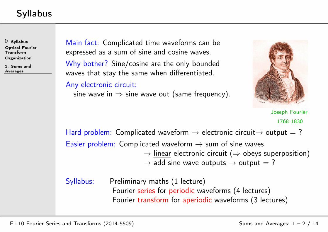
Main fact: Complicated time waveforms can beexpressed as a sum of sine and cosine waves.
Why bother? Sine/cosine are the only boundedwaves that stay the same when differentiated.
Any electronic circuit:sine wave in ⇒ sine wave out (same frequency).
Joseph Fourier
1768-1830
Hard problem: Complicated waveform → electronic circuit→ output = ?
Easier problem: Complicated waveform → sum of sine waves→ linear electronic circuit (⇒ obeys superposition)→ add sine wave outputs → output = ?
Syllabus: Preliminary maths (1 lecture)Fourier series for periodic waveforms (4 lectures)Fourier transform for aperiodic waveforms (3 lectures)

Optical Fourier Transform
Syllabus
⊲Optical FourierTransform
Organization
1: Sums andAverages
E1.10 Fourier Series and Transforms (2014-5509) Sums and Averages: 1 – 3 / 14
A pair of prisms can split light up into its component frequencies (colours).This is called Fourier Analysis.A second pair can re-combine the frequencies.This is called Fourier Synthesis.
Fourier Analysis Fourier Synthesis
We want to do the same thing with mathematical signals instead of light.

Organization
Syllabus
Optical FourierTransform
⊲ Organization
1: Sums andAverages
E1.10 Fourier Series and Transforms (2014-5509) Sums and Averages: 1 – 4 / 14
• 8 lectures: feel free to ask questions
• Textbook: Riley, Hobson & Bence “Mathematical Methods for Physicsand Engineering”, ISBN:978052167971-8, Chapters [4], 12 & 13
• Lecture slides (including animations) and problem sheets + answersavailable via Blackboard or from my website:http://www.ee.ic.ac.uk/hp/staff/dmb/courses/E1Fourier/E1Fourier.htm
• Email me with any errors in slides or problems and if answers arewrong or unclear

1: Sums and Averages
Syllabus
Optical FourierTransform
Organization
⊲1: Sums andAverages
Geometric SeriesInfinite GeometricSeries
Dummy Variables
Dummy VariableSubstitution
Averages
Average Properties
Periodic WaveformsAveraging Sin andCos
Summary
E1.10 Fourier Series and Transforms (2014-5509) Sums and Averages: 1 – 5 / 14

Geometric Series
Syllabus
Optical FourierTransform
Organization
1: Sums andAverages
⊲ Geometric SeriesInfinite GeometricSeries
Dummy Variables
Dummy VariableSubstitution
Averages
Average Properties
Periodic WaveformsAveraging Sin andCos
Summary
E1.10 Fourier Series and Transforms (2014-5509) Sums and Averages: 1 – 6 / 14
A geometric series is a sum of terms that increase or decrease by a constantfactor, x:
S = a+ ax+ ax2 + . . .+ axn
The sequence of terms themselves is called a geometric progression.
We use a trick to get rid of most of the terms:
S = a+ ax+ ax2 + . . .+ axn−1 + axn
xS = ax+ ax2 + ax3 + . . . + axn + axn+1
Now subtract the lines to get: S − xS = (1− x)S = a− axn+1
Divide by 1− x to get: a = first term n+ 1 = number of terms
S = a× 1−xn+1
1−x
Example:S = 3 + 6 + 12 + 24 [a = 3, x = 2, n+ 1 = 4]
= 3× 1−24
1−2 = 3× −15−1 = 45
Infinite Geometric Series
Syllabus
Optical FourierTransform
Organization
1: Sums andAverages
Geometric Series
⊲Infinite GeometricSeries
Dummy Variables
Dummy VariableSubstitution
Averages
Average Properties
Periodic WaveformsAveraging Sin andCos
Summary
E1.10 Fourier Series and Transforms (2014-5509) Sums and Averages: 1 – 7 / 14
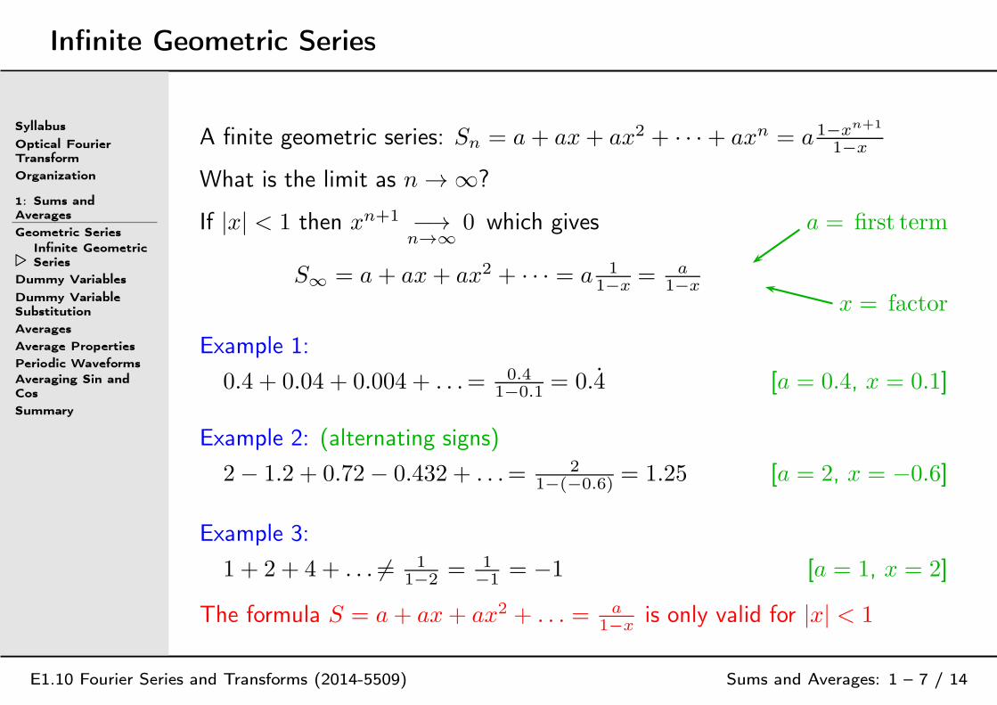
A finite geometric series: Sn = a+ ax+ ax2 + · · ·+ axn = a 1−xn+1
1−x
What is the limit as n → ∞?
If |x| < 1 then xn+1 −→n→∞
0 which gives a = first term
S∞ = a+ ax+ ax2 + · · · = a 11−x
= a1−x
x = factor
Example 1:
0.4 + 0.04 + 0.004 + . . .= 0.41−0.1 = 0.4 [a = 0.4, x = 0.1]
Example 2: (alternating signs)
2− 1.2 + 0.72− 0.432 + . . .= 21−(−0.6) = 1.25 [a = 2, x = −0.6]
Example 3:
1 + 2 + 4 + . . . 6= 11−2 = 1
−1 = −1 [a = 1, x = 2]
The formula S = a+ ax+ ax2 + . . . = a1−x
is only valid for |x| < 1

Dummy Variables
Syllabus
Optical FourierTransform
Organization
1: Sums andAverages
Geometric SeriesInfinite GeometricSeries
⊲ Dummy Variables
Dummy VariableSubstitution
Averages
Average Properties
Periodic WaveformsAveraging Sin andCos
Summary
E1.10 Fourier Series and Transforms (2014-5509) Sums and Averages: 1 – 8 / 14
Using a∑
sign, we can write the geometric series more compactly:
Sn = a+ ax+ ax2 + . . .+ axn=∑n
r=0 axr
[Note: x0 , 1 in this context even when x = 0]
Here r is a dummy variable: you can replace it with anything else∑n
r=0 axr =
∑n
k=0 axk =
∑n
α=0 axα
Dummy variables are undefined outside the summation so they sometimesget re-used elsewhere in an expression:
∑3r=0 2
r +∑2
r=1 3r =
(
1× 1−24
1−2
)
+(
3× 1−32
1−3
)
= 15 + 12 = 27
The two dummy variables are both called r but they have no connectionwith each other at all (or with any other variable called r anywhere else).
Dummy Variable Substitution
Syllabus
Optical FourierTransform
Organization
1: Sums andAverages
Geometric SeriesInfinite GeometricSeries
Dummy Variables
⊲Dummy VariableSubstitution
Averages
Average Properties
Periodic WaveformsAveraging Sin andCos
Summary
E1.10 Fourier Series and Transforms (2014-5509) Sums and Averages: 1 – 9 / 14
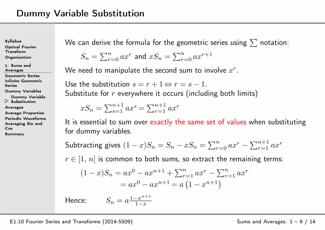
We can derive the formula for the geometric series using∑
notation:
Sn =∑n
r=0 axr and xSn =
∑n
r=0 axr+1
We need to manipulate the second sum to involve xr.
Use the substitution s = r + 1⇔ r = s− 1.Substitute for r everywhere it occurs (including both limits)
xSn =∑n+1
s=1 axs =∑n+1
r=1 axr
It is essential to sum over exactly the same set of values when substitutingfor dummy variables.
Subtracting gives (1− x)Sn = Sn − xSn =∑n
r=0 axr −
∑n+1r=1 ax
r
r ∈ [1, n] is common to both sums, so extract the remaining terms:
(1− x)Sn = ax0 − axn+1 +∑n
r=1 axr −
∑n
r=1 axr
= ax0 − axn+1 = a(
1− xn+1)
Hence: Sn = a 1−xn+1
1−x

Averages
Syllabus
Optical FourierTransform
Organization
1: Sums andAverages
Geometric SeriesInfinite GeometricSeries
Dummy Variables
Dummy VariableSubstitution
⊲ Averages
Average Properties
Periodic WaveformsAveraging Sin andCos
Summary
E1.10 Fourier Series and Transforms (2014-5509) Sums and Averages: 1 – 10 / 14
If a signal varies with time, we can plot its waveform, x(t).
The average value of x(t) in the range T1 ≤ t ≤ T2 is
〈x〉[T1,T2]= 1
T2−T1
∫ T2
t=T1x(t)dt
T1 T
2
x(t)<x>
[T1,T2]
T1 T
2
x(t)<x>
[T1,T2]
The area under the curve x(t) is equal to the area of the rectangledefined by 0 and 〈x〉[T1,T2]
.
Angle brackets alone, 〈x〉, denotes the average value over all time
〈x(t)〉 = limA,B→∞ 〈x(t)〉[−A,+B]

Average Properties
Syllabus
Optical FourierTransform
Organization
1: Sums andAverages
Geometric SeriesInfinite GeometricSeries
Dummy Variables
Dummy VariableSubstitution
Averages
⊲ Average Properties
Periodic WaveformsAveraging Sin andCos
Summary
E1.10 Fourier Series and Transforms (2014-5509) Sums and Averages: 1 – 11 / 14
The properties of averages follow from the properties of integrals:
Addition: 〈x(t) + y(t)〉 = 〈x(t)〉+ 〈y(t)〉
Add a constant: 〈x(t) + c〉 = 〈x(t)〉+ c
Constant multiple: 〈a× x(t)〉 = a× 〈x(t)〉
where the constants a and c do not depend on time.
For example:
〈x(t) + y(t)〉[T1,T2]= 1
T2−T1
∫ T2
t=T1(x(t) + y(t)) dt
= 1T2−T1
∫ T2
t=T1x(t)dt+ 1
T2−T1
∫ T2
t=T1y(t)dt
= 〈x(t)〉[T1,T2]+ 〈y(t)〉[T1,T2]
But beware: 〈x(t)× y(t)〉 6= 〈x(t)〉 × 〈y(t)〉.

Periodic Waveforms
Syllabus
Optical FourierTransform
Organization
1: Sums andAverages
Geometric SeriesInfinite GeometricSeries
Dummy Variables
Dummy VariableSubstitution
Averages
Average Properties
⊲PeriodicWaveforms
Averaging Sin andCos
Summary
E1.10 Fourier Series and Transforms (2014-5509) Sums and Averages: 1 – 12 / 14
A periodic waveform with period T repeats itself at intervals of T :x(t+ T ) = x(t) ⇒ x(t± kT ) = x(t) for any integer k.
The smallest T > 0 for which x(t+ T ) = x(t) ∀t is the fundamentalperiod. The fundamental frequency is F = 1
T.
T
<x>
For a periodic waveform, 〈x(t)〉 equals the average over one period.It doesn’t make any difference where in a period you start or how manywhole periods you take the average over.
Example:x(t) = |sin t|
〈x〉 = 1π
∫ π
t=0|sin t| dt= 1
π
∫ π
t=0sin t dt
= 1π[− cos t]
π
0 =1π(1 + 1) = 2
π≈ 0.637
[proof that x(t± kT ) = x(t)]
E1.10 Fourier Series and Transforms (2014-5509) Sums and Averages: 1 – note 1 of slide 12
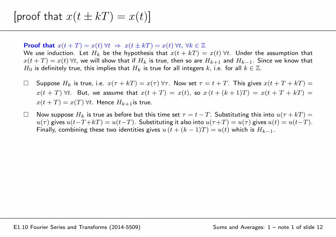
Proof that x(t+ T ) = x(t) ∀t ⇒ x(t± kT ) = x(t) ∀t, ∀k ∈ Z
We use induction. Let Hk be the hypothesis that x(t + kT ) = x(t) ∀t. Under the assumption that
x(t+ T ) = x(t) ∀t, we will show that if Hk is true, then so are Hk+1 and Hk−1. Since we know that
H0 is definitely true, this implies that Hk is true for all integers k, i.e. for all k ∈ Z.
Suppose Hk is true, i.e. x(τ + kT ) = x(τ) ∀τ . Now set τ = t + T . This gives x(t + T + kT ) =
x(t + T ) ∀t. But, we assume that x(t + T ) = x(t), so x (t+ (k + 1)T ) = x(t + T + kT ) =
x(t+ T ) = x(T ) ∀t. Hence Hk+1is true.
Now suppose Hk is true as before but this time set τ = t− T . Substituting this into u(τ + kT ) =u(τ) gives u(t−T+kT ) = u(t−T ). Substituting it also into u(τ+T ) = u(τ) gives u(t) = u(t−T ).Finally, combining these two identities gives u (t+ (k − 1)T ) = u(t) which is Hk−1.
Averaging Sin and Cos
Syllabus
Optical FourierTransform
Organization
1: Sums andAverages
Geometric SeriesInfinite GeometricSeries
Dummy Variables
Dummy VariableSubstitution
Averages
Average Properties
Periodic Waveforms
⊲Averaging Sin andCos
Summary
E1.10 Fourier Series and Transforms (2014-5509) Sums and Averages: 1 – 13 / 14
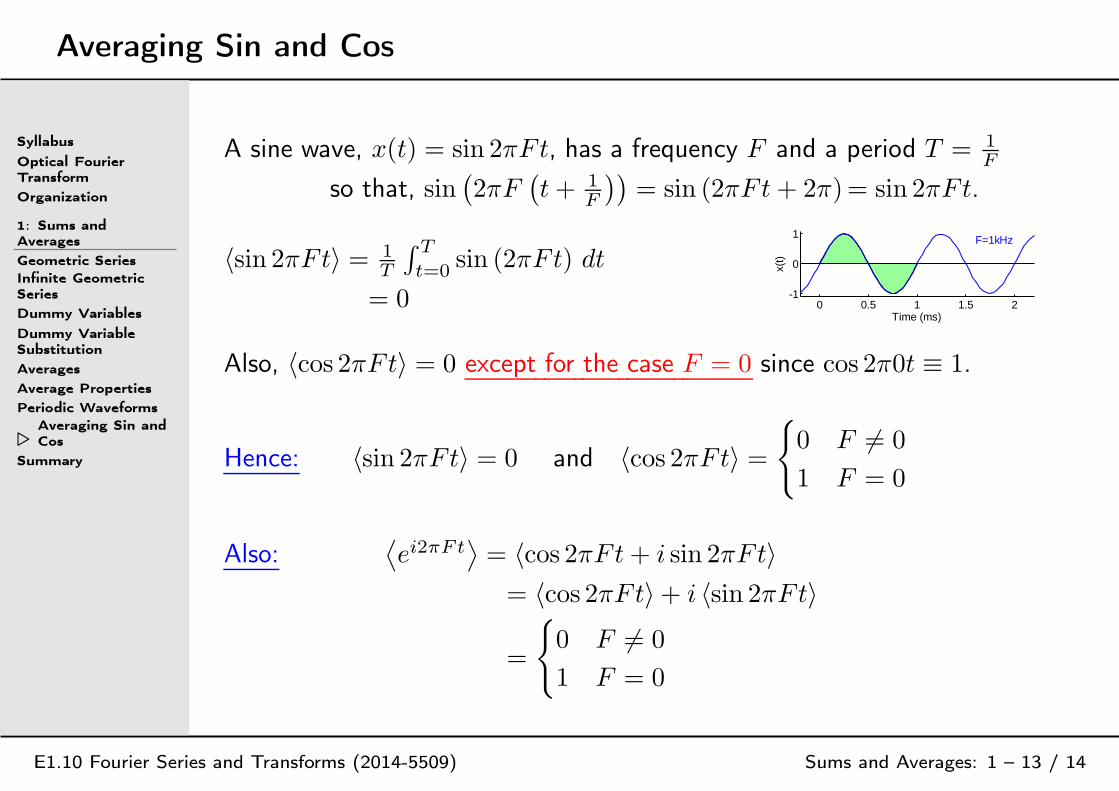
A sine wave, x(t) = sin 2πFt, has a frequency F and a period T = 1F
so that, sin(
2πF(
t+ 1F
))
= sin (2πFt+ 2π)= sin 2πFt.
〈sin 2πFt〉 = 1T
∫ T
t=0sin (2πFt) dt
= 0 0 0.5 1 1.5 2-1
0
1 F=1kHz
x(t)
Time (ms)
Also, 〈cos 2πFt〉 = 0 except for the case F = 0 since cos 2π0t ≡ 1.
Hence: 〈sin 2πFt〉 = 0 and 〈cos 2πFt〉 =
0 F 6= 0
1 F = 0
Also:⟨
ei2πFt⟩
= 〈cos 2πFt+ i sin 2πFt〉
= 〈cos 2πFt〉+ i 〈sin 2πFt〉
=
0 F 6= 0
1 F = 0
Summary
Syllabus
Optical FourierTransform
Organization
1: Sums andAverages
Geometric SeriesInfinite GeometricSeries
Dummy Variables
Dummy VariableSubstitution
Averages
Average Properties
Periodic WaveformsAveraging Sin andCos
⊲ Summary
E1.10 Fourier Series and Transforms (2014-5509) Sums and Averages: 1 – 14 / 14
• Sum of geometric series (see RHB Chapter 4)
Finite series: S = a× 1−xn+1
1−x
Infinite series: S = a1−x
but only if |x| < 1
• Dummy variables Commonly re-used elsewhere in expressions Substitutions must cover exactly the same set of values
• Averages: 〈x〉[T1,T2]= 1
T2−T1
∫ T2
t=T1x(t)dt
• Periodic waveforms: x(t± kT ) = x(t) for any integer k Fundamental period is the smallest T Fundamental frequency is F = 1
T
For periodic waveforms, 〈x〉 is the average over any integernumber of periods
〈sin 2πFt〉 = 0
〈cos 2πFt〉 =⟨
ei2πFt⟩
=
0 F 6= 0
1 F = 0
2: Fourier Series
⊲ 2: Fourier Series
Periodic Functions
Fourier SeriesWhy Sin and CosWaves?
Dirichlet Conditions
Fourier Analysis
TrigonometricProducts
Fourier Analysis
Fourier AnalysisExample
Linearity
Summary
E1.10 Fourier Series and Transforms (2014-5379) Fourier Series: 2 – 1 / 11

Periodic Functions
2: Fourier Series
⊲ Periodic Functions
Fourier SeriesWhy Sin and CosWaves?
Dirichlet Conditions
Fourier Analysis
TrigonometricProducts
Fourier Analysis
Fourier AnalysisExample
Linearity
Summary
E1.10 Fourier Series and Transforms (2014-5379) Fourier Series: 2 – 2 / 11
A function, u(t), is periodic with period T if u(t+ T ) = u(t) ∀t• Periodic with period T ⇒ Periodic with period kT ∀k ∈ Z
+
The fundamental period is the smallest T > 0 for which u(t+ T ) = u(t) T
If you add together functions with different periods the fundamental periodis the lowest common multiple (LCM) of the individual fundamentalperiods.
Example:• u(t) = cos 4πt ⇒ Tu = 2π
4π= 0.5
• v(t) = cos 5πt ⇒ Tv = 2π
5π= 0.4
• w(t) = u(t) + 0.1v(t) ⇒ Tw = lcm(0.5, 0.4) = 2.0 T
u = 0.5 T
v = 0.4 T
w = 2.0
Fourier Series
2: Fourier Series
Periodic Functions
⊲ Fourier SeriesWhy Sin and CosWaves?
Dirichlet Conditions
Fourier Analysis
TrigonometricProducts
Fourier Analysis
Fourier AnalysisExample
Linearity
Summary
E1.10 Fourier Series and Transforms (2014-5379) Fourier Series: 2 – 3 / 11
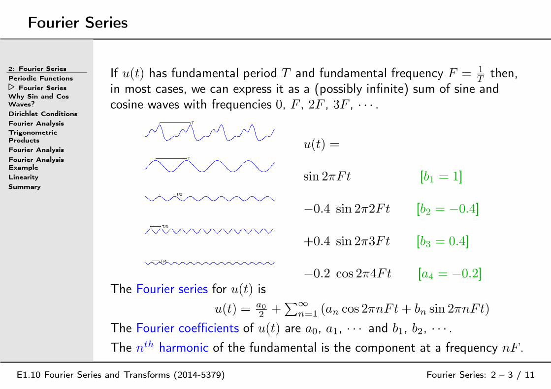
If u(t) has fundamental period T and fundamental frequency F = 1
Tthen,
in most cases, we can express it as a (possibly infinite) sum of sine andcosine waves with frequencies 0, F , 2F , 3F , · · · .
T
u(t) = T
sin 2πFt [b1 = 1] T/2
−0.4 sin 2π2Ft [b2 = −0.4] T/3
+0.4 sin 2π3Ft [b3 = 0.4]
T/4
−0.2 cos 2π4Ft [a4 = −0.2]The Fourier series for u(t) is
u(t) = a0
2+∑
∞
n=1(an cos 2πnFt+ bn sin 2πnFt)
The Fourier coefficients of u(t) are a0, a1, · · · and b1, b2, · · · .
The nth harmonic of the fundamental is the component at a frequency nF .

Why Sin and Cos Waves?
2: Fourier Series
Periodic Functions
Fourier Series
⊲Why Sin and CosWaves?
Dirichlet Conditions
Fourier Analysis
TrigonometricProducts
Fourier Analysis
Fourier AnalysisExample
Linearity
Summary
E1.10 Fourier Series and Transforms (2014-5379) Fourier Series: 2 – 4 / 11
Why are engineers obsessed with sine waves?Answer: Because ...
1. A sine wave remains a sine wave of the same frequency when you(a) multiply by a constant,(b) add onto to another sine wave of the same frequency,(c) differentiate or integrate or shift in time
2. Almost any function can be expressed as a sum of sine waves Periodic functions → Fourier Series Aperiodic functions → Fourier Transform
3. Many physical and electronic systems are(a) composed entirely of constant-multiply/add/differentiate(b) linear: u(t) → x(t) and v(t) → y(t)
means that u(t) + v(t) → x(t) + y(t)⇒ sum of sine waves → sum of sine waves
In these lectures we will use T for the fundamental period and F = 1
Tfor
the fundamental frequency.
Dirichlet Conditions
2: Fourier Series
Periodic Functions
Fourier SeriesWhy Sin and CosWaves?
⊲DirichletConditions
Fourier Analysis
TrigonometricProducts
Fourier Analysis
Fourier AnalysisExample
Linearity
Summary
E1.10 Fourier Series and Transforms (2014-5379) Fourier Series: 2 – 5 / 11
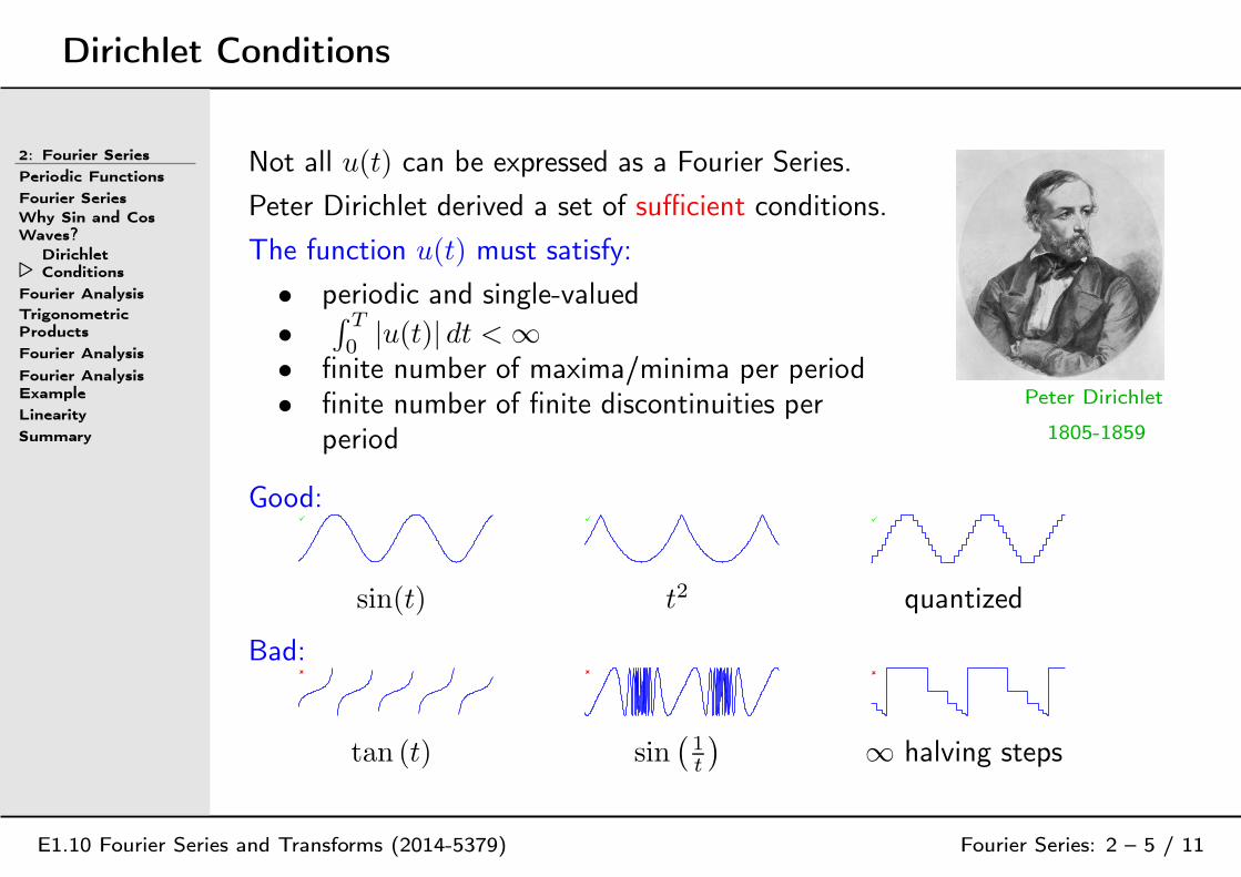
Not all u(t) can be expressed as a Fourier Series.
Peter Dirichlet derived a set of sufficient conditions.
The function u(t) must satisfy:
• periodic and single-valued
•∫ T
0|u(t)| dt < ∞
• finite number of maxima/minima per period• finite number of finite discontinuities per
period
Peter Dirichlet
1805-1859
Good:
sin(t) t2 quantized
Bad:
tan (t) sin(
1
t
)
∞ halving steps
Fourier Analysis
2: Fourier Series
Periodic Functions
Fourier SeriesWhy Sin and CosWaves?
Dirichlet Conditions
⊲ Fourier Analysis
TrigonometricProducts
Fourier Analysis
Fourier AnalysisExample
Linearity
Summary
E1.10 Fourier Series and Transforms (2014-5379) Fourier Series: 2 – 6 / 11
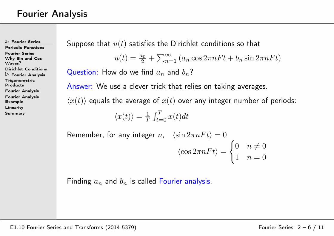
Suppose that u(t) satisfies the Dirichlet conditions so that
u(t) = a0
2+∑
∞
n=1(an cos 2πnFt+ bn sin 2πnFt)
Question: How do we find an and bn?
Answer: We use a clever trick that relies on taking averages.
〈x(t)〉 equals the average of x(t) over any integer number of periods:
〈x(t)〉 = 1
T
∫ T
t=0x(t)dt
Remember, for any integer n, 〈sin 2πnFt〉 = 0
〈cos 2πnFt〉 =
0 n 6= 0
1 n = 0
Finding an and bn is called Fourier analysis.
Trigonometric Products
2: Fourier Series
Periodic Functions
Fourier SeriesWhy Sin and CosWaves?
Dirichlet Conditions
Fourier Analysis
⊲TrigonometricProducts
Fourier Analysis
Fourier AnalysisExample
Linearity
Summary
E1.10 Fourier Series and Transforms (2014-5379) Fourier Series: 2 – 7 / 11
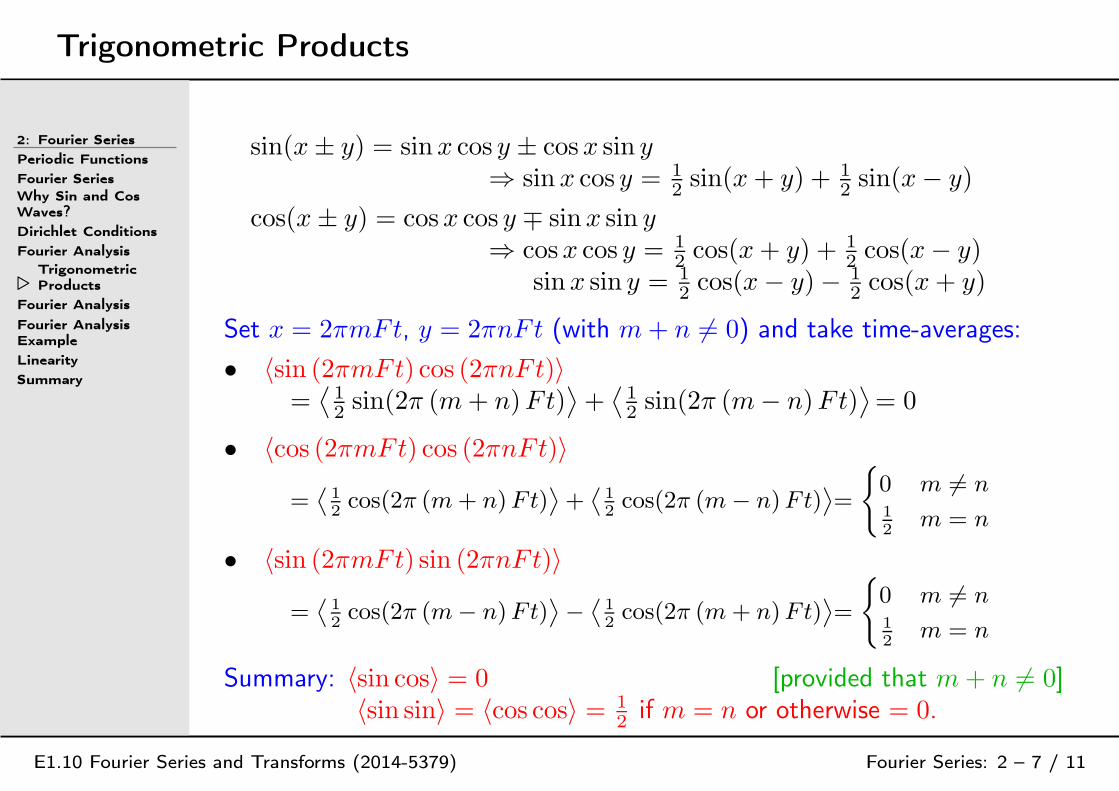
sin(x± y) = sinx cos y ± cosx sin y⇒ sin x cos y = 1
2sin(x+ y) + 1
2sin(x− y)
cos(x± y) = cosx cos y ∓ sinx sin y⇒ cosx cos y = 1
2cos(x+ y) + 1
2cos(x− y)
sinx sin y = 1
2cos(x− y)− 1
2cos(x+ y)
Set x = 2πmFt, y = 2πnFt (with m+ n 6= 0) and take time-averages:
• 〈sin (2πmFt) cos (2πnFt)〉=
⟨
1
2sin(2π (m+ n)Ft)
⟩
+⟨
1
2sin(2π (m− n)Ft)
⟩
= 0
• 〈cos (2πmFt) cos (2πnFt)〉
=⟨
1
2cos(2π (m+ n)Ft)
⟩
+⟨
1
2cos(2π (m− n)Ft)
⟩
=
0 m 6= n
1
2m = n
• 〈sin (2πmFt) sin (2πnFt)〉
=⟨
1
2cos(2π (m− n)Ft)
⟩
−⟨
1
2cos(2π (m+ n)Ft)
⟩
=
0 m 6= n
1
2m = n
Summary: 〈sin cos〉 = 0 [provided that m+ n 6= 0]〈sin sin〉 = 〈cos cos〉 = 1
2if m = n or otherwise = 0.
[Trigonometric Products Proofs]
E1.10 Fourier Series and Transforms (2014-5379) Fourier Series: 2 – note 1 of slide 7
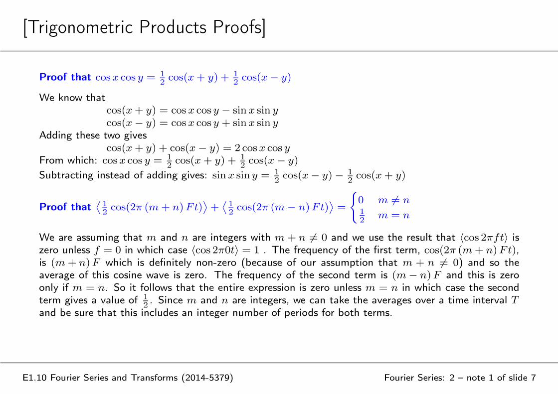
Proof that cosx cos y = 1
2cos(x+ y) + 1
2cos(x− y)
We know thatcos(x+ y) = cosx cos y − sinx sin y
cos(x− y) = cosx cos y + sinx sin y
Adding these two givescos(x+ y) + cos(x− y) = 2 cosx cos y
From which: cosx cos y = 1
2cos(x+ y) + 1
2cos(x− y)
Subtracting instead of adding gives: sinx sin y = 1
2cos(x− y)− 1
2cos(x+ y)
Proof that⟨
1
2cos(2π (m+ n)Ft)
⟩
+⟨
1
2cos(2π (m− n)Ft)
⟩
=
0 m 6= n1
2m = n
We are assuming that m and n are integers with m + n 6= 0 and we use the result that 〈cos 2πft〉 iszero unless f = 0 in which case 〈cos 2π0t〉 = 1 . The frequency of the first term, cos(2π (m+ n)Ft),is (m+ n)F which is definitely non-zero (because of our assumption that m + n 6= 0) and so theaverage of this cosine wave is zero. The frequency of the second term is (m− n)F and this is zeroonly if m = n. So it follows that the entire expression is zero unless m = n in which case the secondterm gives a value of 1
2. Since m and n are integers, we can take the averages over a time interval T
and be sure that this includes an integer number of periods for both terms.
Fourier Analysis
2: Fourier Series
Periodic Functions
Fourier SeriesWhy Sin and CosWaves?
Dirichlet Conditions
Fourier Analysis
TrigonometricProducts
⊲ Fourier Analysis
Fourier AnalysisExample
Linearity
Summary
E1.10 Fourier Series and Transforms (2014-5379) Fourier Series: 2 – 8 / 11
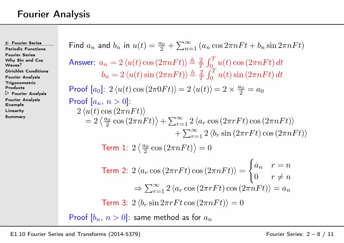
Find an and bn in u(t) = a0
2+∑
∞
n=1(an cos 2πnFt+ bn sin 2πnFt)
Answer: an = 2 〈u(t) cos (2πnFt)〉, 2
T
∫ T
0u(t) cos (2πnFt) dt
bn = 2 〈u(t) sin (2πnFt)〉, 2
T
∫ T
0u(t) sin (2πnFt) dt
Proof [a0]: 2 〈u(t) cos (2π0Ft)〉= 2 〈u(t)〉= 2× a0
2= a0
Proof [an, n > 0]:2 〈u(t) cos (2πnFt)〉= 2
⟨
a0
2cos (2πnFt)
⟩
+∑
∞
r=12 〈ar cos (2πrFt) cos (2πnFt)〉
+∑
∞
r=12 〈br sin (2πrFt) cos (2πnFt)〉
Term 1: 2⟨
a0
2cos (2πnFt)
⟩
= 0
Term 2: 2 〈ar cos (2πrFt) cos (2πnFt)〉 =
an r = n
0 r 6= n
⇒∑
∞
r=12 〈ar cos (2πrFt) cos (2πnFt)〉 = an
Term 3: 2 〈br sin 2πrFt cos (2πnFt)〉 = 0
Proof [bn, n > 0]: same method as for an
Fourier Analysis Example
2: Fourier Series
Periodic Functions
Fourier SeriesWhy Sin and CosWaves?
Dirichlet Conditions
Fourier Analysis
TrigonometricProducts
Fourier Analysis
⊲Fourier AnalysisExample
Linearity
Summary
E1.10 Fourier Series and Transforms (2014-5379) Fourier Series: 2 – 9 / 11
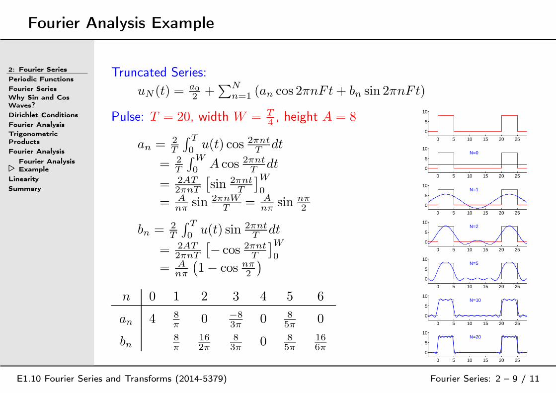
Truncated Series:
uN (t) = a0
2+∑N
n=1(an cos 2πnFt+ bn sin 2πnFt)
Pulse: T = 20, width W = T
4, height A = 8
an = 2
T
∫ T
0u(t) cos 2πnt
Tdt
= 2
T
∫W
0A cos 2πnt
Tdt
= 2AT
2πnT
[
sin 2πnt
T
]W
0
= A
nπsin 2πnW
T= A
nπsin nπ
2
bn = 2
T
∫ T
0u(t) sin 2πnt
Tdt
= 2AT
2πnT
[
− cos 2πnt
T
]W
0
= A
nπ
(
1− cos nπ
2
)
n 0 1 2 3 4 5 6
an 4 8
π0 −8
3π0 8
5π0
bn8
π
16
2π
8
3π0 8
5π
16
6π
0 5 10 15 20 25
0
5
10
0 5 10 15 20 25
0
5
10N=0
0 5 10 15 20 25
0
5
10N=1
0 5 10 15 20 25
0
5
10N=2
0 5 10 15 20 25
0
5
10N=5
0 5 10 15 20 25
0
5
10N=10
0 5 10 15 20 25
0
5
10N=20
[Small Angle Approximation]
E1.10 Fourier Series and Transforms (2014-5379) Fourier Series: 2 – note 1 of slide 9
In the previous example, we can obtain a0 by noting that a0
2= 〈u(t)〉, the average value of the
waveform which must be AW
T= 2. From this, a0 = 4. We can, however, also derive this value from
the general expression.The expression for am is am = A
nπsin nπ
2. For the case, n = 0, this is difficult to evaluate because both
the numerator and denominator are zero. The general way of dealing with this situation is L’Hôpital’srule (see section 4.7 of RHB) but here we can use a simpler and very useful technique that is oftenreferred to as the “small angle approximation”. For small values of θ we can approximate the standardtrigonometrical functions as: sin θ ≈ θ, cos θ ≈ 1 − 0.5θ2 and tan θ ≈ θ. These approximations areobtained by taking the first three terms of the Taylor series; they are accurate to O(θ3) and are exactlycorrect when θ = 0. When m = 0 we can therefore make an exact approximation to an by writingan = A
nπsin nπ
2≈ A
nπ× nπ
2= A
2= 4. What we have implicitly done here is to assume that n is a
real number (instead of an integer) and then taken the limit of an as n → 0.
Linearity
2: Fourier Series
Periodic Functions
Fourier SeriesWhy Sin and CosWaves?
Dirichlet Conditions
Fourier Analysis
TrigonometricProducts
Fourier Analysis
Fourier AnalysisExample
⊲ Linearity
Summary
E1.10 Fourier Series and Transforms (2014-5379) Fourier Series: 2 – 10 / 11
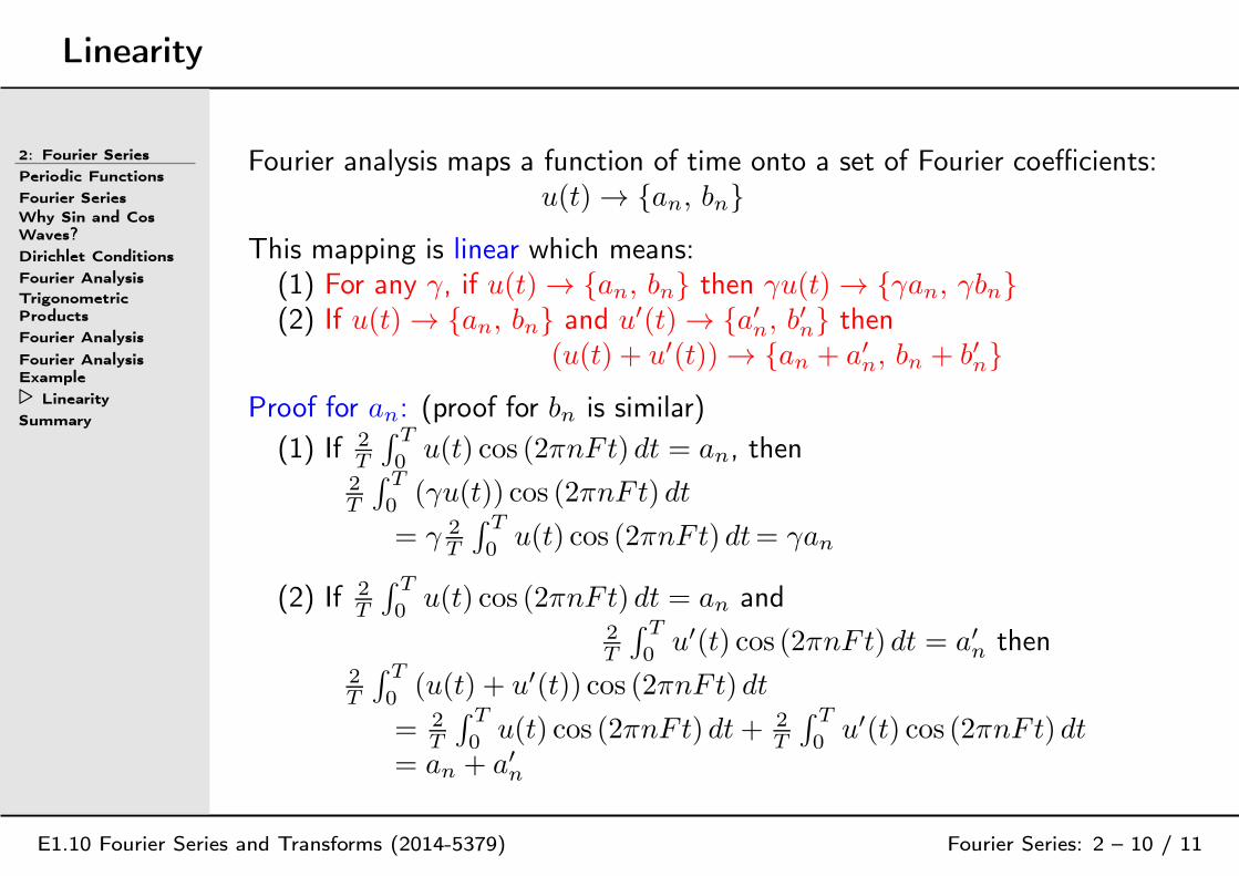
Fourier analysis maps a function of time onto a set of Fourier coefficients:u(t) → an, bn
This mapping is linear which means:(1) For any γ, if u(t) → an, bn then γu(t) → γan, γbn(2) If u(t) → an, bn and u′(t) → a′n, b
′
n then(u(t) + u′(t)) → an + a′n, bn + b′n
Proof for an: (proof for bn is similar)
(1) If 2
T
∫ T
0u(t) cos (2πnFt) dt = an, then
2
T
∫ T
0(γu(t)) cos (2πnFt) dt
= γ 2
T
∫ T
0u(t) cos (2πnFt) dt= γan
(2) If 2
T
∫ T
0u(t) cos (2πnFt) dt = an and
2
T
∫ T
0u′(t) cos (2πnFt) dt = a′n then
2
T
∫ T
0(u(t) + u′(t)) cos (2πnFt) dt
= 2
T
∫ T
0u(t) cos (2πnFt) dt+ 2
T
∫ T
0u′(t) cos (2πnFt) dt
= an + a′n

Summary
2: Fourier Series
Periodic Functions
Fourier SeriesWhy Sin and CosWaves?
Dirichlet Conditions
Fourier Analysis
TrigonometricProducts
Fourier Analysis
Fourier AnalysisExample
Linearity
⊲ Summary
E1.10 Fourier Series and Transforms (2014-5379) Fourier Series: 2 – 11 / 11
• Fourier Series:u(t) = a0
2+∑
∞
n=1(an cos 2πnFt+ bn sin 2πnFt)
• Dirichlet Conditions: sufficient conditions for FS to exist Periodic, Single-valued, Bounded absolute integral Finite number of (a) max/min and (b) finite discontinuities
• Fourier Analysis = “finding an and bn”
an = 2 〈u(t) cos (2πnFt)〉
, 2
T
∫ T
0u(t) cos (2πnFt) dt
bn = 2 〈u(t) sin (2πnFt)〉
, 2
T
∫ T
0u(t) sin (2πnFt) dt
• The mapping u(t) → an, bn is linear
For further details see RHB 12.1 and 12.2.

3: Complex Fourier Series
⊲3: ComplexFourier Series
Euler’s Equation
Complex FourierSeriesAveraging ComplexExponentials
Complex FourierAnalysisFourier Series ↔
Complex FourierSeriesComplex FourierAnalysis Example
Time Shifting
Even/Odd Symmetry
Antiperiodic ⇒ OddHarmonics Only
Symmetry Examples
Summary
E1.10 Fourier Series and Transforms (2014-5543) Complex Fourier Series: 3 – 1 / 12

Euler’s Equation
3: Complex FourierSeries
⊲ Euler’s Equation
Complex FourierSeriesAveraging ComplexExponentials
Complex FourierAnalysisFourier Series ↔
Complex FourierSeriesComplex FourierAnalysis Example
Time Shifting
Even/Odd Symmetry
Antiperiodic ⇒ OddHarmonics Only
Symmetry Examples
Summary
E1.10 Fourier Series and Transforms (2014-5543) Complex Fourier Series: 3 – 2 / 12
Euler’s Equation: eiθ = cos θ + i sin θ [see RHB 3.3]
Hence: cos θ = eiθ+e−iθ
2 = 12e
iθ + 12e
−iθ
sin θ = eiθ−e−iθ
2i = − 12 ie
iθ + 12 ie
−iθ
Most maths becomes simpler if you use eiθ instead of cos θ and sin θ
The Complex Fourier Series is the Fourier Series but written using eiθ
Examples where using eiθ makes things simpler:
Using eiθ Using cos θ and sin θ
ei(θ+φ) = eiθeiφ cos (θ + φ) = cos θ cosφ− sin θ sinφ
eiθeiφ = ei(θ+φ) cos θ cosφ = 12 cos (θ + φ) + 1
2 cos (θ − φ)
ddθeiθ = ieiθ d
dθcos θ = − sin θ
Complex Fourier Series
3: Complex FourierSeries
Euler’s Equation
⊲Complex FourierSeries
Averaging ComplexExponentials
Complex FourierAnalysisFourier Series ↔
Complex FourierSeriesComplex FourierAnalysis Example
Time Shifting
Even/Odd Symmetry
Antiperiodic ⇒ OddHarmonics Only
Symmetry Examples
Summary
E1.10 Fourier Series and Transforms (2014-5543) Complex Fourier Series: 3 – 3 / 12
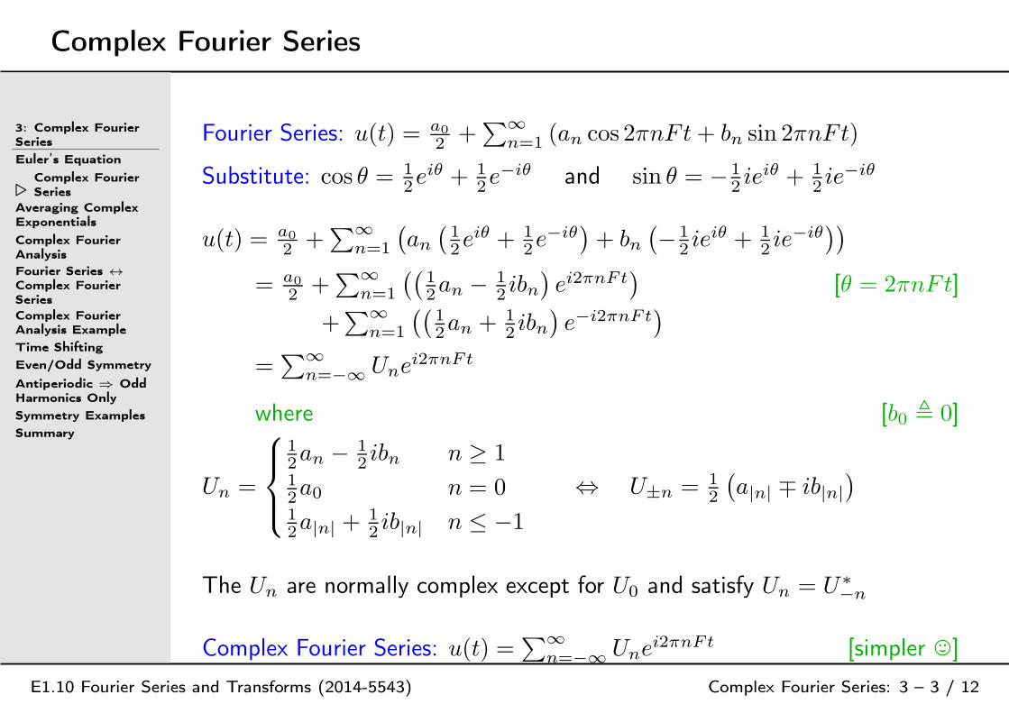
Fourier Series: u(t) = a0
2 +∑∞
n=1 (an cos 2πnFt+ bn sin 2πnFt)
Substitute: cos θ = 12e
iθ + 12e
−iθ and sin θ = − 12 ie
iθ + 12 ie
−iθ
u(t) = a0
2 +∑∞
n=1
(
an(
12e
iθ + 12e
−iθ)
+ bn(
− 12 ie
iθ + 12 ie
−iθ))
= a0
2 +∑∞
n=1
((
12an − 1
2 ibn)
ei2πnFt)
[θ = 2πnFt]
+∑∞
n=1
((
12an + 1
2 ibn)
e−i2πnFt)
=∑∞
n=−∞ Unei2πnFt
where [b0 , 0]
Un =
12an − 1
2 ibn n ≥ 112a0 n = 012a|n| +
12 ib|n| n ≤ −1
⇔ U±n = 12
(
a|n| ∓ ib|n|)
The Un are normally complex except for U0 and satisfy Un = U∗−n
Complex Fourier Series: u(t) =∑∞
n=−∞ Unei2πnFt [simpler ,]
Averaging Complex Exponentials
3: Complex FourierSeries
Euler’s Equation
Complex FourierSeries
⊲Averaging ComplexExponentials
Complex FourierAnalysisFourier Series ↔
Complex FourierSeriesComplex FourierAnalysis Example
Time Shifting
Even/Odd Symmetry
Antiperiodic ⇒ OddHarmonics Only
Symmetry Examples
Summary
E1.10 Fourier Series and Transforms (2014-5543) Complex Fourier Series: 3 – 4 / 12
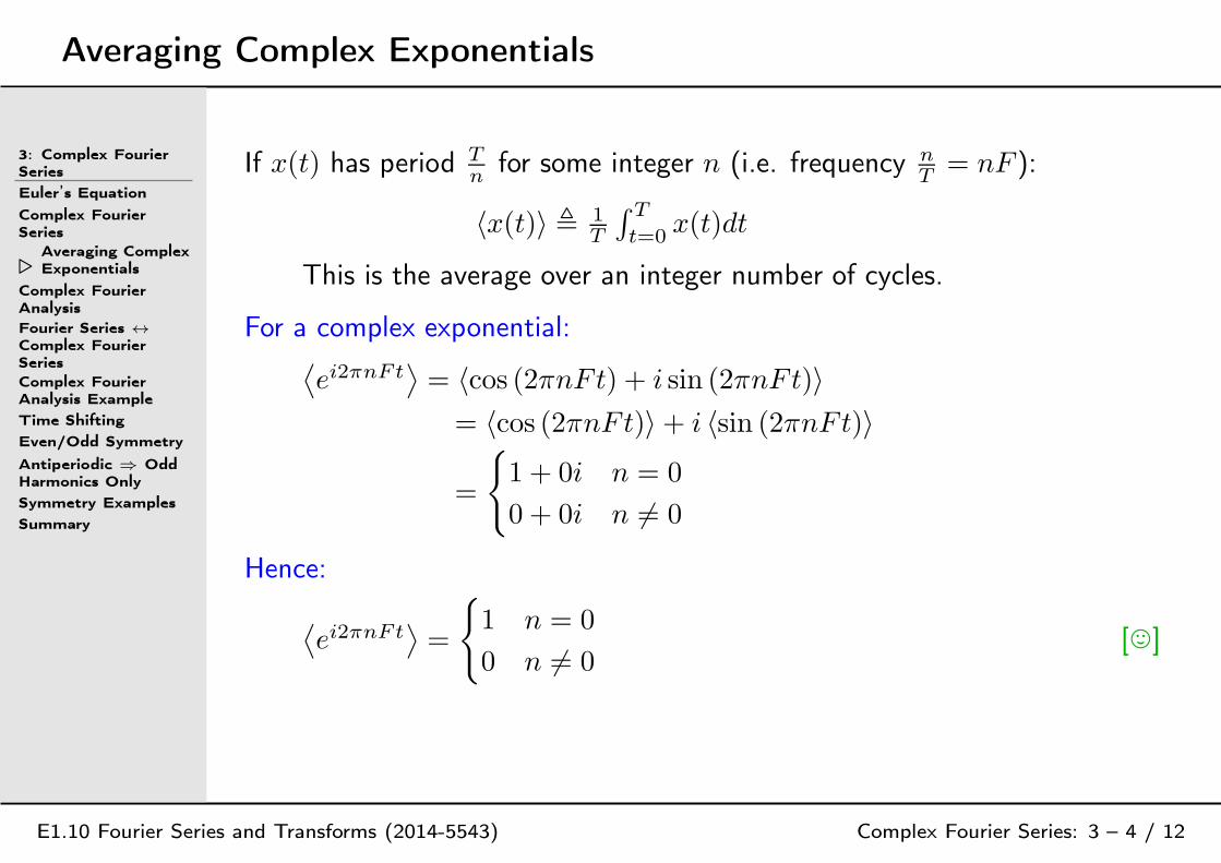
If x(t) has period Tn
for some integer n (i.e. frequency nT= nF ):
〈x(t)〉 , 1T
∫ T
t=0x(t)dt
This is the average over an integer number of cycles.
For a complex exponential:⟨
ei2πnFt⟩
= 〈cos (2πnFt) + i sin (2πnFt)〉
= 〈cos (2πnFt)〉+ i 〈sin (2πnFt)〉
=
1 + 0i n = 0
0 + 0i n 6= 0
Hence:
⟨
ei2πnFt⟩
=
1 n = 0
0 n 6= 0[,]

Complex Fourier Analysis
3: Complex FourierSeries
Euler’s Equation
Complex FourierSeriesAveraging ComplexExponentials
⊲Complex FourierAnalysis
Fourier Series ↔
Complex FourierSeriesComplex FourierAnalysis Example
Time Shifting
Even/Odd Symmetry
Antiperiodic ⇒ OddHarmonics Only
Symmetry Examples
Summary
E1.10 Fourier Series and Transforms (2014-5543) Complex Fourier Series: 3 – 5 / 12
Complex Fourier Series: u(t) =∑∞
n=−∞ Unei2πnFt
To find the coefficient, Un, we multiply by something that makes all theterms involving the other coefficients average to zero.⟨
u(t)e−i2πnFt⟩
=⟨∑∞
r=−∞ Urei2πrFte−i2πnFt
⟩
=⟨∑∞
r=−∞ Urei2π(r−n)Ft
⟩
=∑∞
r=−∞ Ur
⟨
ei2π(r−n)Ft⟩
All terms in the sum are zero, except for the one when n = r which equalsUn:
Un =⟨
u(t)e−i2πnFt⟩
[,]
This shows that the Fourier series coefficients are unique: you cannot havetwo different sets of coefficients that result in the same function u(t).
Note the sign of the exponent: “+” in the Fourier Series but “−” forFourier Analysis (in order to cancel out the “+”).

Fourier Series ↔ Complex Fourier Series
3: Complex FourierSeries
Euler’s Equation
Complex FourierSeriesAveraging ComplexExponentials
Complex FourierAnalysis
⊲
Fourier Series ↔
Complex FourierSeries
Complex FourierAnalysis Example
Time Shifting
Even/Odd Symmetry
Antiperiodic ⇒ OddHarmonics Only
Symmetry Examples
Summary
E1.10 Fourier Series and Transforms (2014-5543) Complex Fourier Series: 3 – 6 / 12
u(t) = a0
2 +∑∞
n=1 (an cos 2πnFt+ bn sin 2πnFt)
=∑∞
n=−∞ Unei2πnFt
We can easily convert between the two forms.
Fourier Coefficients → Complex Fourier Coefficients:
U±n = 12
(
a|n| ∓ ib|n|)
[Un = U∗−n]
Complex Fourier Coefficients → Fourier Coefficients:
an = Un + U−n = 2ℜ (Un) [ℜ = “real part”]
bn = i (Un − U−n) = −2ℑ (Un) [ℑ = “imaginary part”]
The formula for an works even for n = 0.

[Complex functions of time]
E1.10 Fourier Series and Transforms (2014-5543) Complex Fourier Series: 3 – note 1 of slide 6
In these lectures, we are assuming that u(t) is a periodic real-valued function of time. In this case we
can represent u(t) using either the Fourier Series or the Complex Fourier Series:
u(t) = a0
2+
∑∞
n=1(an cos 2πnFt+ bn sin 2πnFt) =
∑∞
n=−∞Une
i2πnFt
We have seen that the Un coefficients are complex-valued and that Un and U−n are complex conjugates
so that we can write U−n = U∗
n.
In fact, the complex Fourier series can also be used when u(t) is a complex-valued function of time(this is sometimes useful in the fields of communications and signal processing). In this case, it is stilltrue that u(t) =
∑∞
n=−∞Une
i2πnFt, but now Un and U−n are completely independent and normallyU−n 6= U∗
n.
Complex Fourier Analysis Example
3: Complex FourierSeries
Euler’s Equation
Complex FourierSeriesAveraging ComplexExponentials
Complex FourierAnalysisFourier Series ↔
Complex FourierSeries
⊲Complex FourierAnalysis Example
Time Shifting
Even/Odd Symmetry
Antiperiodic ⇒ OddHarmonics Only
Symmetry Examples
Summary
E1.10 Fourier Series and Transforms (2014-5543) Complex Fourier Series: 3 – 7 / 12
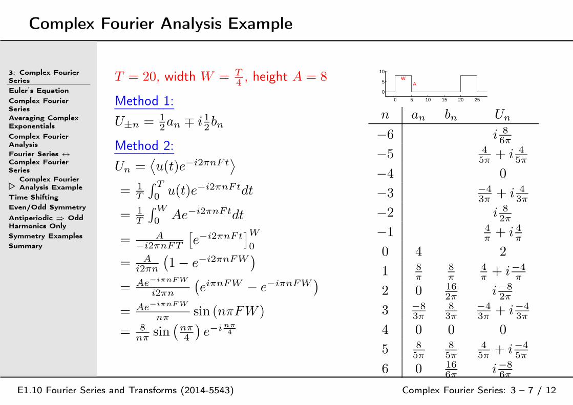
T = 20, width W = T4 , height A = 8
Method 1:
U±n = 12an ∓ i 12bn
Method 2:
Un =⟨
u(t)e−i2πnFt⟩
= 1T
∫ T
0u(t)e−i2πnFtdt
= 1T
∫W
0Ae−i2πnFtdt
= A−i2πnFT
[
e−i2πnFt]W
0
= Ai2πn
(
1− e−i2πnFW)
= Ae−iπnFW
i2πn
(
eiπnFW − e−iπnFW)
= Ae−iπnFW
nπsin (nπFW )
= 8nπ
sin(
nπ4
)
e−inπ
4
0 5 10 15 20 25
0
5
10W
A
n an bn Un
−6 i 86π
−5 45π + i 4
5π
−4 0
−3 −43π + i 4
3π
−2 i 82π
−1 4π+ i 4
π
0 4 2
1 8π
8π
4π+ i−4
π
2 0 162π i−8
2π
3 −83π
83π
−43π + i−4
3π
4 0 0 0
5 85π
85π
45π + i−4
5π
6 0 166π i−8
6π

Time Shifting
3: Complex FourierSeries
Euler’s Equation
Complex FourierSeriesAveraging ComplexExponentials
Complex FourierAnalysisFourier Series ↔
Complex FourierSeriesComplex FourierAnalysis Example
⊲ Time Shifting
Even/Odd Symmetry
Antiperiodic ⇒ OddHarmonics Only
Symmetry Examples
Summary
E1.10 Fourier Series and Transforms (2014-5543) Complex Fourier Series: 3 – 8 / 12
Complex Fourier Series: u(t) =∑∞
n=−∞ Unei2πnFt
If v(t) is the same as u(t) but delayed by a time τ : v(t) = u(t− τ )
v(t) =∑∞
n=−∞ Unei2πnF (t−τ) =
∑∞n=−∞
(
Une−i2πnFτ
)
ei2πnFt
=∑∞
n=−∞ Vnei2πnFt
where Vn = Une−i2πnFτ
Example:u(t) = 6 cos (2πFt)
Fourier: a1 = 6, b1 = 0
Complex: U±1 = 12a1 ∓
12 ib1 = 3
v(t) = 6 sin (2πFt)= u(t− τ )
Time delay: τ = T4 ⇒ Fτ = 1
4
Complex: V1 = U1e−iπ
2 = −3i
V−1 = U−1eiπ
2 = +3i
0 0.5 1 1.5 2-5
0
5u(t)
0 0.5 1 1.5 2-5
0
5v(t)
Note: If u(t) is a sine wave, U1 equals half the corresponding phasor.
Even/Odd Symmetry
3: Complex FourierSeries
Euler’s Equation
Complex FourierSeriesAveraging ComplexExponentials
Complex FourierAnalysisFourier Series ↔
Complex FourierSeriesComplex FourierAnalysis Example
Time Shifting
⊲Even/OddSymmetry
Antiperiodic ⇒ OddHarmonics Only
Symmetry Examples
Summary
E1.10 Fourier Series and Transforms (2014-5543) Complex Fourier Series: 3 – 9 / 12
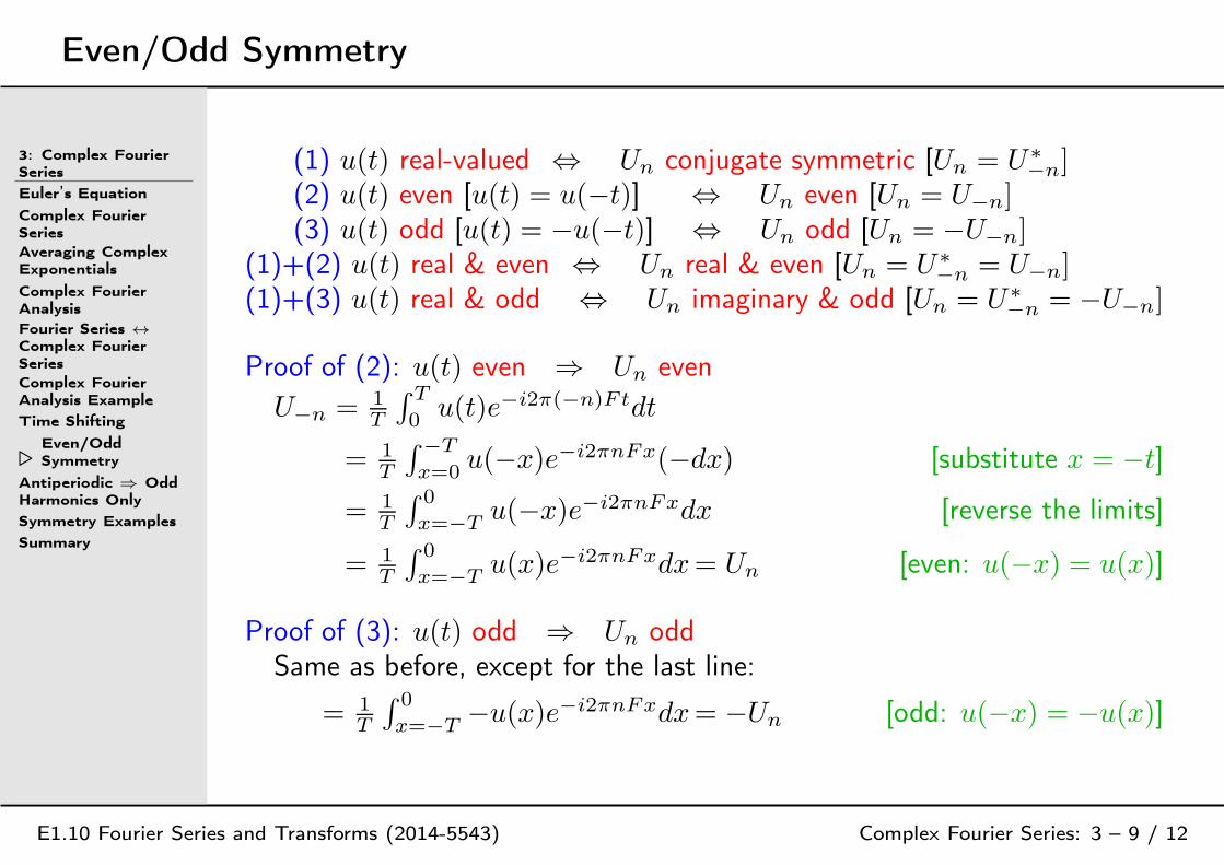
(1) u(t) real-valued ⇔ Un conjugate symmetric [Un = U∗−n]
(2) u(t) even [u(t) = u(−t)] ⇔ Un even [Un = U−n](3) u(t) odd [u(t) = −u(−t)] ⇔ Un odd [Un = −U−n]
(1)+(2) u(t) real & even ⇔ Un real & even [Un = U∗−n = U−n]
(1)+(3) u(t) real & odd ⇔ Un imaginary & odd [Un = U∗−n = −U−n]
Proof of (2): u(t) even ⇒ Un even
U−n = 1T
∫ T
0u(t)e−i2π(−n)Ftdt
= 1T
∫ −T
x=0u(−x)e−i2πnFx(−dx) [substitute x = −t]
= 1T
∫ 0
x=−Tu(−x)e−i2πnFxdx [reverse the limits]
= 1T
∫ 0
x=−Tu(x)e−i2πnFxdx= Un [even: u(−x) = u(x)]
Proof of (3): u(t) odd ⇒ Un oddSame as before, except for the last line:
= 1T
∫ 0
x=−T−u(x)e−i2πnFxdx= −Un [odd: u(−x) = −u(x)]

Antiperiodic ⇒ Odd Harmonics Only
3: Complex FourierSeries
Euler’s Equation
Complex FourierSeriesAveraging ComplexExponentials
Complex FourierAnalysisFourier Series ↔
Complex FourierSeriesComplex FourierAnalysis Example
Time Shifting
Even/Odd Symmetry
⊲
Antiperiodic ⇒
Odd HarmonicsOnly
Symmetry Examples
Summary
E1.10 Fourier Series and Transforms (2014-5543) Complex Fourier Series: 3 – 10 / 12
A waveform, u(t), is anti-periodic if u(t+ 12T ) = −u(t).
If u(t) is anti-periodic then Un = 0 for n even.
Proof:
Define v(t) = u(t+ T2 ), then
(1) v(t) = −u(t)⇒ Vn = −Un
(2) v(t) equals u(t) but delayed by −T2
⇒ Vn = Unei2πnF T
2 = Uneinπ =
Un n even
−Un n odd
Hence for n even: Vn = −Un = Un ⇒ Un = 0
Example:
U0:5 = [0, 3 + 2i, 0, i, 0, 1]Odd harmonics only ⇔Second half of each period is thenegative of the first half.
-1 -0.5 0 0.5 1
-5
0
5
U[0:5]=[0, 3+2j, 0, j, 0, 1]

Symmetry Examples
3: Complex FourierSeries
Euler’s Equation
Complex FourierSeriesAveraging ComplexExponentials
Complex FourierAnalysisFourier Series ↔
Complex FourierSeriesComplex FourierAnalysis Example
Time Shifting
Even/Odd Symmetry
Antiperiodic ⇒ OddHarmonics Only
⊲SymmetryExamples
Summary
E1.10 Fourier Series and Transforms (2014-5543) Complex Fourier Series: 3 – 11 / 12
All these examples assume that u(t) is real-valued ⇔ U−n = U∗+n.
(1) Even u(t) ⇔ real Un
U0:2 = [0, 2, −1]
-1 -0.5 0 0.5 1-6-4-202
U[0:2]=[0, 2, -1]
(2) Odd u(t) ⇔ imaginary Un
U0:3 = [0, −2i, i, i]
-1 -0.5 0 0.5 1
-5
0
5
U[0:3]=[0, -2j, j, j]
(3) Anti-periodic u(t)⇔ odd harmonics only
U0:1 = [0, −i]-1 -0.5 0 0.5 1
-2
0
2U[0:1]=[0, -j]
(4) Even harmonics only⇔ period is really 1
2T
U0:4 = [2, 0, 2, 0, 1]-1 -0.5 0 0.5 1
02468
U[0:4]=[2, 0, 2, 0, 1]
Summary
3: Complex FourierSeries
Euler’s Equation
Complex FourierSeriesAveraging ComplexExponentials
Complex FourierAnalysisFourier Series ↔
Complex FourierSeriesComplex FourierAnalysis Example
Time Shifting
Even/Odd Symmetry
Antiperiodic ⇒ OddHarmonics Only
Symmetry Examples
⊲ Summary
E1.10 Fourier Series and Transforms (2014-5543) Complex Fourier Series: 3 – 12 / 12
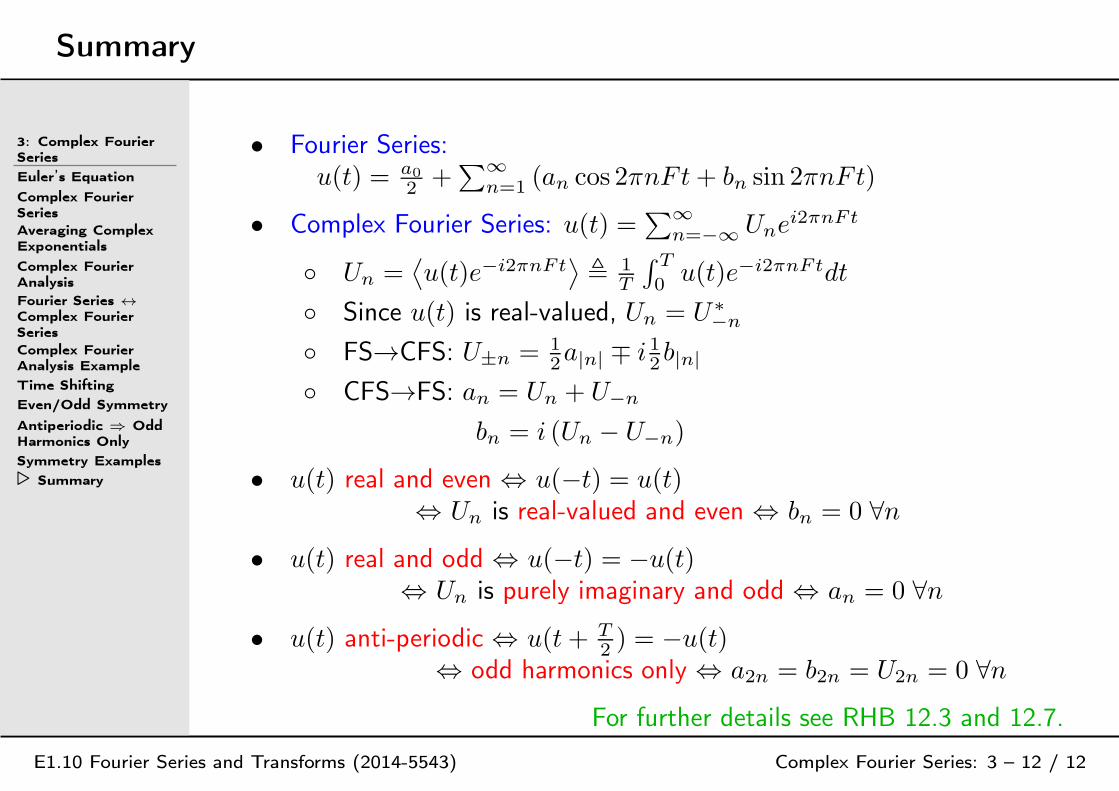
• Fourier Series:u(t) = a0
2 +∑∞
n=1 (an cos 2πnFt+ bn sin 2πnFt)
• Complex Fourier Series: u(t) =∑∞
n=−∞ Unei2πnFt
Un =⟨
u(t)e−i2πnFt⟩
, 1T
∫ T
0u(t)e−i2πnFtdt
Since u(t) is real-valued, Un = U∗−n
FS→CFS: U±n = 12a|n| ∓ i 12b|n|
CFS→FS: an = Un + U−n
bn = i (Un − U−n)
• u(t) real and even ⇔ u(−t) = u(t)⇔ Un is real-valued and even ⇔ bn = 0 ∀n
• u(t) real and odd ⇔ u(−t) = −u(t)⇔ Un is purely imaginary and odd ⇔ an = 0 ∀n
• u(t) anti-periodic ⇔ u(t+ T2 ) = −u(t)
⇔ odd harmonics only ⇔ a2n = b2n = U2n = 0 ∀n
For further details see RHB 12.3 and 12.7.
4: Parseval’s Theorem and Convolution
⊲
4: Parseval’sTheorem andConvolution
Parseval’s Theorem(a.k.a. Plancherel’sTheorem)
Power ConservationMagnitude Spectrumand Power Spectrum
Product of Signals
ConvolutionProperties
Convolution Example
Convolution andPolynomialMultiplication
Summary
E1.10 Fourier Series and Transforms (2014-5543) Parseval and Convolution: 4 – 1 / 9
Parseval’s Theorem (a.k.a. Plancherel’s Theorem)
4: Parseval’sTheorem andConvolution
⊲
Parseval’sTheorem (a.k.a.Plancherel’sTheorem)
Power ConservationMagnitude Spectrumand Power Spectrum
Product of Signals
ConvolutionProperties
Convolution Example
Convolution andPolynomialMultiplication
Summary
E1.10 Fourier Series and Transforms (2014-5543) Parseval and Convolution: 4 – 2 / 9
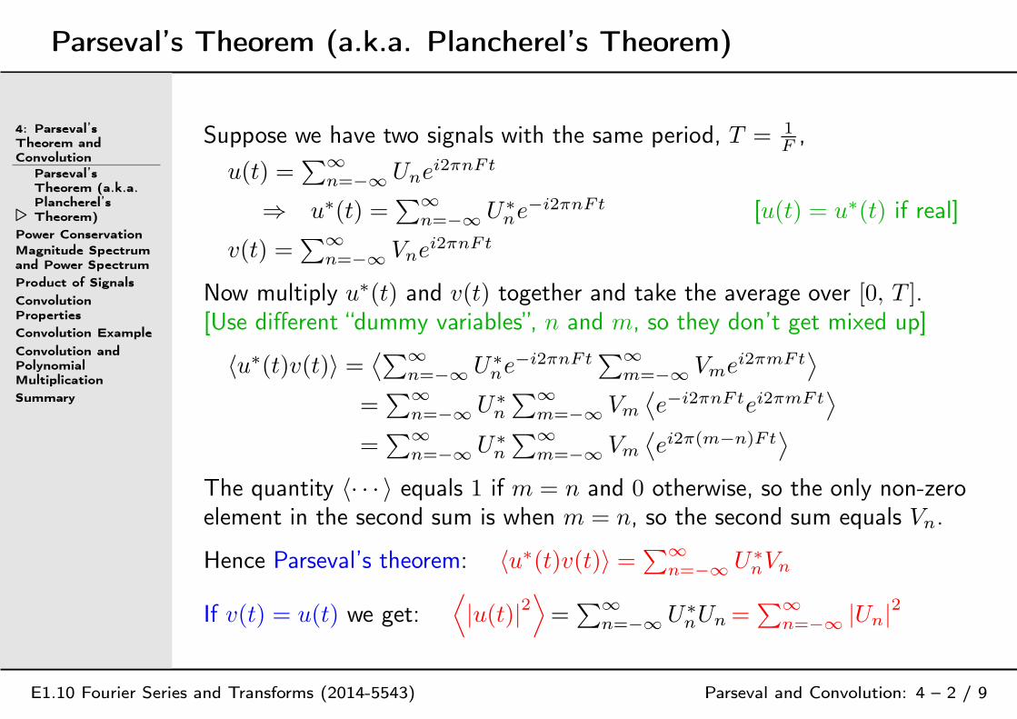
Suppose we have two signals with the same period, T = 1F
,
u(t) =∑∞
n=−∞ Unei2πnFt
⇒ u∗(t) =∑∞
n=−∞ U∗ne−i2πnFt [u(t) = u∗(t) if real]
v(t) =∑∞
n=−∞ Vnei2πnFt
Now multiply u∗(t) and v(t) together and take the average over [0, T ].[Use different “dummy variables”, n and m, so they don’t get mixed up]
〈u∗(t)v(t)〉 =⟨∑∞
n=−∞ U∗ne−i2πnFt
∑∞m=−∞ Vmei2πmFt
⟩
=∑∞
n=−∞ U∗n
∑∞m=−∞ Vm
⟨
e−i2πnFtei2πmFt⟩
=∑∞
n=−∞ U∗n
∑∞m=−∞ Vm
⟨
ei2π(m−n)Ft⟩
The quantity 〈· · · 〉 equals 1 if m = n and 0 otherwise, so the only non-zeroelement in the second sum is when m = n, so the second sum equals Vn.
Hence Parseval’s theorem: 〈u∗(t)v(t)〉 = ∑∞n=−∞ U∗
nVn
If v(t) = u(t) we get:⟨
|u(t)|2⟩
=∑∞
n=−∞ U∗nUn =
∑∞n=−∞ |Un|2
[Manipulating sums]
E1.10 Fourier Series and Transforms (2014-5543) Parseval and Convolution: 4 – note 1 of slide 2
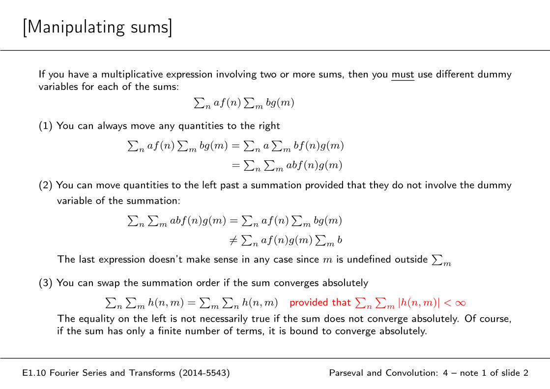
If you have a multiplicative expression involving two or more sums, then you must use different dummyvariables for each of the sums:
∑naf(n)
∑m
bg(m)
(1) You can always move any quantities to the right∑
naf(n)
∑m
bg(m) =∑
na∑
mbf(n)g(m)
=∑
n
∑m
abf(n)g(m)
(2) You can move quantities to the left past a summation provided that they do not involve the dummy
variable of the summation:∑
n
∑m
abf(n)g(m) =∑
naf(n)
∑m
bg(m)
6=∑
naf(n)g(m)
∑m
b
The last expression doesn’t make sense in any case since m is undefined outside∑
m
(3) You can swap the summation order if the sum converges absolutely∑
n
∑m
h(n,m) =∑
m
∑nh(n,m) provided that
∑n
∑m
|h(n,m)| < ∞
The equality on the left is not necessarily true if the sum does not converge absolutely. Of course,if the sum has only a finite number of terms, it is bound to converge absolutely.
Power Conservation
4: Parseval’sTheorem andConvolutionParseval’s Theorem(a.k.a. Plancherel’sTheorem)
⊲PowerConservation
Magnitude Spectrumand Power Spectrum
Product of Signals
ConvolutionProperties
Convolution Example
Convolution andPolynomialMultiplication
Summary
E1.10 Fourier Series and Transforms (2014-5543) Parseval and Convolution: 4 – 3 / 9
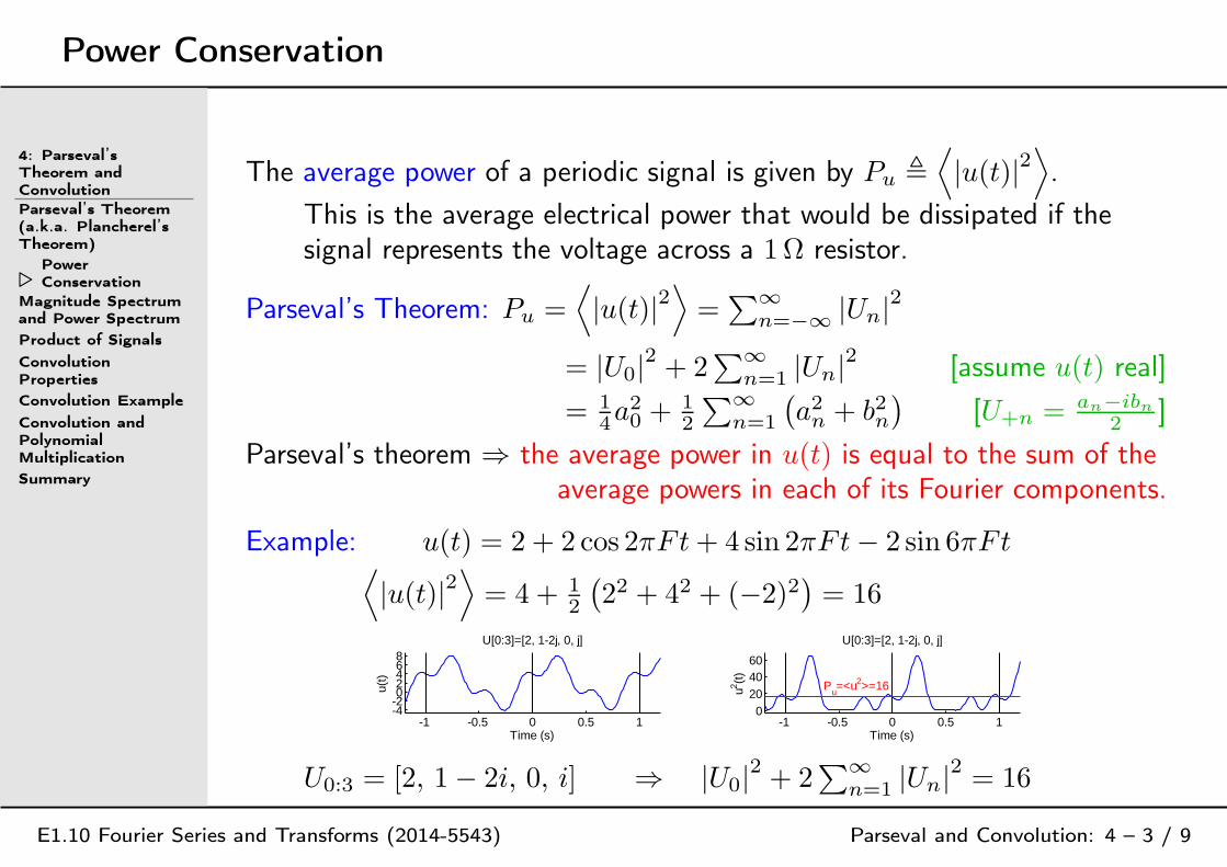
The average power of a periodic signal is given by Pu ,
⟨
|u(t)|2⟩
.
This is the average electrical power that would be dissipated if thesignal represents the voltage across a 1Ω resistor.
Parseval’s Theorem: Pu =⟨
|u(t)|2⟩
=∑∞
n=−∞ |Un|2
= |U0|2 + 2∑∞
n=1 |Un|2 [assume u(t) real]
= 14a
20 +
12
∑∞n=1
(
a2n+ b2
n
)
[U+n = an−ibn
2 ]
Parseval’s theorem ⇒ the average power in u(t) is equal to the sum of theaverage powers in each of its Fourier components.
Example: u(t) = 2 + 2 cos 2πFt+ 4 sin 2πFt− 2 sin 6πFt⟨
|u(t)|2⟩
= 4 + 12
(
22 + 42 + (−2)2)
= 16
-1 -0.5 0 0.5 1-4-202468
u(t)
U[0:3]=[2, 1-2j, 0, j]
Time (s)-1 -0.5 0 0.5 1
0204060
u2 (t)
Pu=<u2>=16
U[0:3]=[2, 1-2j, 0, j]
Time (s)
U0:3 = [2, 1− 2i, 0, i] ⇒ |U0|2 + 2∑∞
n=1 |Un|2 = 16

Magnitude Spectrum and Power Spectrum
4: Parseval’sTheorem andConvolutionParseval’s Theorem(a.k.a. Plancherel’sTheorem)
Power Conservation
⊲
MagnitudeSpectrum andPower Spectrum
Product of Signals
ConvolutionProperties
Convolution Example
Convolution andPolynomialMultiplication
Summary
E1.10 Fourier Series and Transforms (2014-5543) Parseval and Convolution: 4 – 4 / 9
The spectrum of a periodic signal is the values of Un versus nF .
The magnitude spectrum is the values of |Un| =
12
√
a2|n| + b2|n|
.
The power spectrum is the values of
|Un|2
=
14
(
a2|n| + b2|n|
)
.
Example:u(t) = 2 + 2 cos 2πFt+ 4 sin 2πFt− 2 sin 6πFt
Fourier Coefficients: a0:3 = [4, 2, 0, 0] b1:3 = [4, 0, −2]
Spectrum: U−3:3 = [−i, 0, 1 + 2i, 2, 1− 2i, 0, i]
Magnitude Spectrum: |U−3:3| =[
1, 0,√5, 2,
√5, 0, 1
]
Power Spectrum:∣
∣U2−3:3
∣
∣ = [1, 0, 5, 4, 5, 0, 1] [∑
=⟨
u2(t)⟩
]
-3 -2 -1 0 1 2 30
1
2
Frequency (Hz)
|Un|
-3 -2 -1 0 1 2 30
5
Frequency (Hz)|U
n2 |
Σ=16
The magnitude and power spectra of a real periodic signal are symmetrical.
A one-sided power power spectrum shows U0 and then 2 |Un|2 for n ≥ 1.
Product of Signals
4: Parseval’sTheorem andConvolutionParseval’s Theorem(a.k.a. Plancherel’sTheorem)
Power ConservationMagnitude Spectrumand Power Spectrum
⊲ Product of Signals
ConvolutionProperties
Convolution Example
Convolution andPolynomialMultiplication
Summary
E1.10 Fourier Series and Transforms (2014-5543) Parseval and Convolution: 4 – 5 / 9
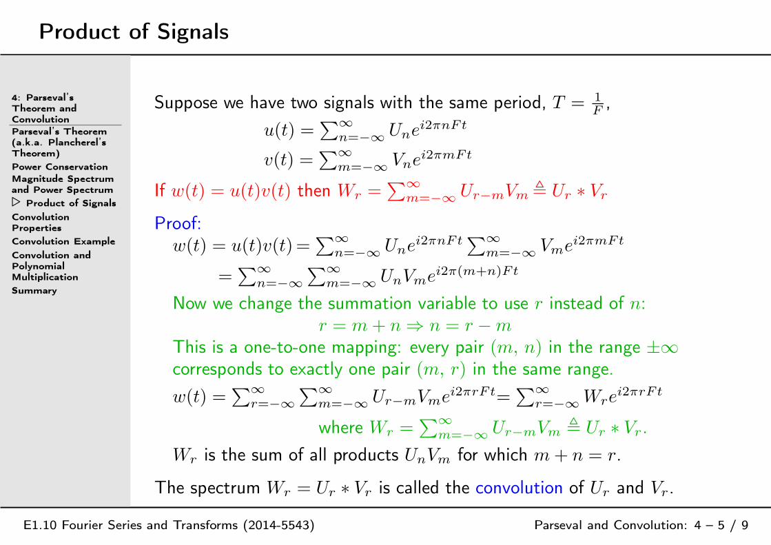
Suppose we have two signals with the same period, T = 1F
,
u(t) =∑∞
n=−∞ Unei2πnFt
v(t) =∑∞
m=−∞ Vnei2πmFt
If w(t) = u(t)v(t) then Wr =∑∞
m=−∞ Ur−mVm , Ur ∗ Vr
Proof:w(t) = u(t)v(t)=
∑∞n=−∞ Une
i2πnFt∑∞
m=−∞ Vmei2πmFt
=∑∞
n=−∞
∑∞m=−∞ UnVmei2π(m+n)Ft
Now we change the summation variable to use r instead of n:r = m+ n ⇒ n = r −m
This is a one-to-one mapping: every pair (m, n) in the range ±∞corresponds to exactly one pair (m, r) in the same range.
w(t) =∑∞
r=−∞
∑∞m=−∞ Ur−mVmei2πrFt=
∑∞r=−∞Wre
i2πrFt
where Wr =∑∞
m=−∞ Ur−mVm , Ur ∗ Vr.
Wr is the sum of all products UnVm for which m+ n = r.
The spectrum Wr = Ur ∗ Vr is called the convolution of Ur and Vr.
Convolution Properties
4: Parseval’sTheorem andConvolutionParseval’s Theorem(a.k.a. Plancherel’sTheorem)
Power ConservationMagnitude Spectrumand Power Spectrum
Product of Signals
⊲ConvolutionProperties
Convolution Example
Convolution andPolynomialMultiplication
Summary
E1.10 Fourier Series and Transforms (2014-5543) Parseval and Convolution: 4 – 6 / 9
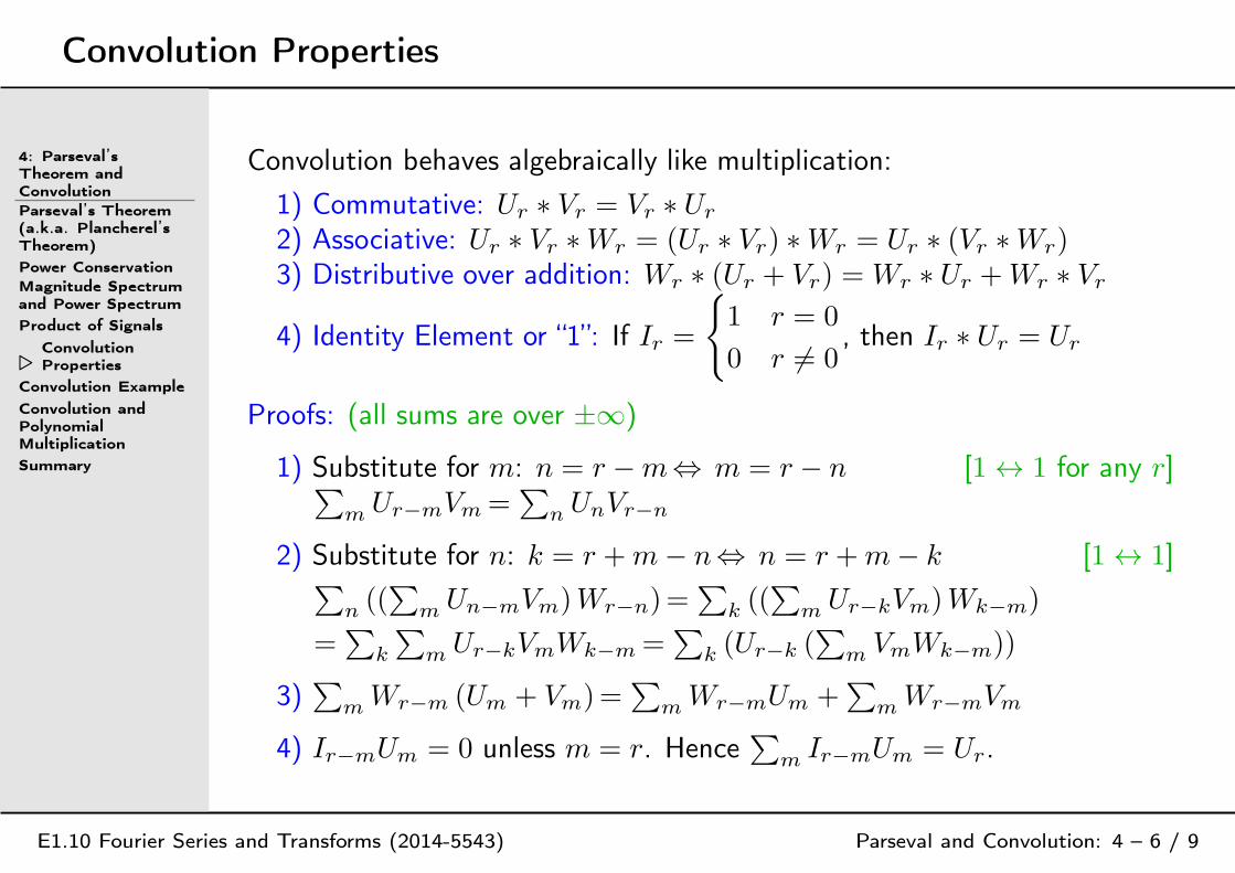
Convolution behaves algebraically like multiplication:
1) Commutative: Ur ∗ Vr = Vr ∗ Ur
2) Associative: Ur ∗ Vr ∗Wr = (Ur ∗ Vr) ∗Wr = Ur ∗ (Vr ∗Wr)3) Distributive over addition: Wr ∗ (Ur + Vr) = Wr ∗ Ur +Wr ∗ Vr
4) Identity Element or “1”: If Ir =
1 r = 0
0 r 6= 0, then Ir ∗ Ur = Ur
Proofs: (all sums are over ±∞)
1) Substitute for m: n = r −m⇔ m = r − n [1 ↔ 1 for any r]∑
mUr−mVm=
∑
nUnVr−n
2) Substitute for n: k = r +m− n⇔ n = r +m− k [1 ↔ 1]∑
n((∑
mUn−mVm)Wr−n)=
∑
k((∑
mUr−kVm)Wk−m)
=∑
k
∑
mUr−kVmWk−m=
∑
k(Ur−k (
∑
mVmWk−m))
3)∑
mWr−m (Um + Vm)=
∑
mWr−mUm +
∑
mWr−mVm
4) Ir−mUm = 0 unless m = r. Hence∑
mIr−mUm = Ur.
Convolution Example
4: Parseval’sTheorem andConvolutionParseval’s Theorem(a.k.a. Plancherel’sTheorem)
Power ConservationMagnitude Spectrumand Power Spectrum
Product of Signals
ConvolutionProperties
⊲ConvolutionExample
Convolution andPolynomialMultiplication
Summary
E1.10 Fourier Series and Transforms (2014-5543) Parseval and Convolution: 4 – 7 / 9
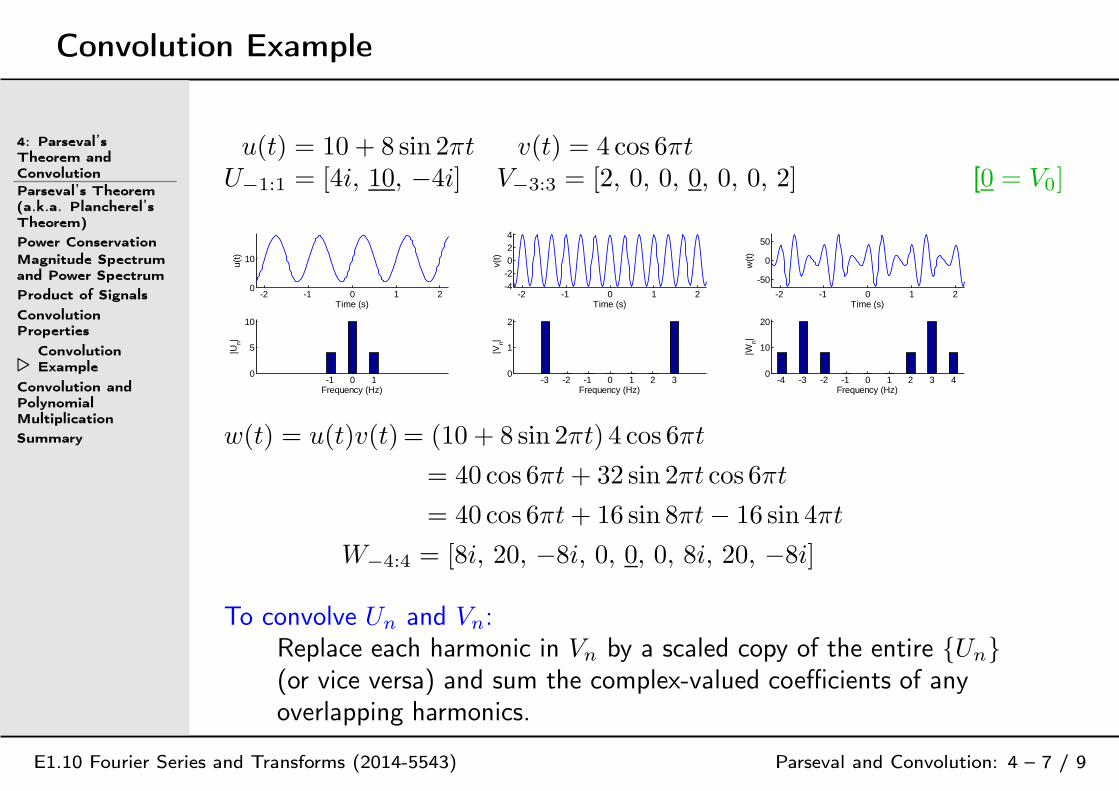
u(t) = 10 + 8 sin 2πt v(t) = 4 cos 6πtU−1:1 = [4i, 10, −4i] V−3:3 = [2, 0, 0, 0, 0, 0, 2] [0 = V0]
-2 -1 0 1 20
10
u(t)
Time (s)-2 -1 0 1 2
-4-2024
v(t)
Time (s)-2 -1 0 1 2
-50
0
50
w(t
)
Time (s)
-1 0 10
5
10
Frequency (Hz)
|Un|
-3 -2 -1 0 1 2 30
1
2
Frequency (Hz)
|Vn|
-4 -3 -2 -1 0 1 2 3 40
10
20
Frequency (Hz)
|Wn|
w(t) = u(t)v(t)= (10 + 8 sin 2πt) 4 cos 6πt
= 40 cos 6πt+ 32 sin 2πt cos 6πt
= 40 cos 6πt+ 16 sin 8πt− 16 sin 4πt
W−4:4 = [8i, 20, −8i, 0, 0, 0, 8i, 20, −8i]
To convolve Un and Vn:Replace each harmonic in Vn by a scaled copy of the entire Un(or vice versa) and sum the complex-valued coefficients of anyoverlapping harmonics.
Convolution and Polynomial Multiplication
4: Parseval’sTheorem andConvolutionParseval’s Theorem(a.k.a. Plancherel’sTheorem)
Power ConservationMagnitude Spectrumand Power Spectrum
Product of Signals
ConvolutionProperties
Convolution Example
⊲
Convolution andPolynomialMultiplication
Summary
E1.10 Fourier Series and Transforms (2014-5543) Parseval and Convolution: 4 – 8 / 9
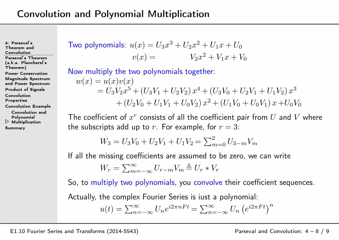
Two polynomials: u(x) = U3x3 + U2x
2 + U1x+ U0
v(x) = V2x2 + V1x+ V0
Now multiply the two polynomials together:w(x) = u(x)v(x)
= U3V2x5 +(U3V1 + U2V2)x
4 +(U3V0 + U2V1 + U1V2)x3
+(U2V0 + U1V1 + U0V2)x2 +(U1V0 + U0V1)x+U0V0
The coefficient of xr consists of all the coefficient pair from U and V wherethe subscripts add up to r. For example, for r = 3:
W3 = U3V0 + U2V1 + U1V2 =∑2
m=0 U3−mVm
If all the missing coefficients are assumed to be zero, we can write
Wr =∑∞
m=−∞ Ur−mVm , Ur ∗ Vr
So, to multiply two polynomials, you convolve their coefficient sequences.
Actually, the complex Fourier Series is iust a polynomial:
u(t) =∑∞
n=−∞ Unei2πnFt =
∑∞n=−∞ Un
(
ei2πFt)n
Summary
4: Parseval’sTheorem andConvolutionParseval’s Theorem(a.k.a. Plancherel’sTheorem)
Power ConservationMagnitude Spectrumand Power Spectrum
Product of Signals
ConvolutionProperties
Convolution Example
Convolution andPolynomialMultiplication
⊲ Summary
E1.10 Fourier Series and Transforms (2014-5543) Parseval and Convolution: 4 – 9 / 9
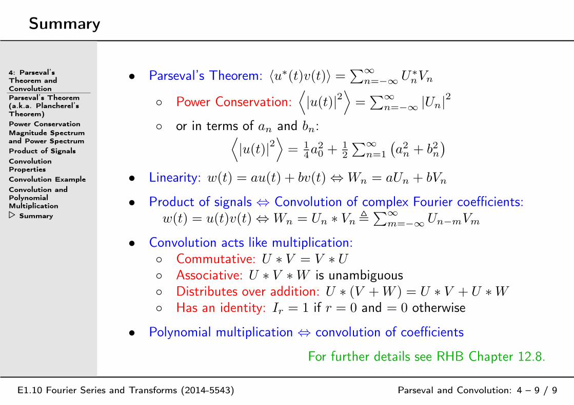
• Parseval’s Theorem: 〈u∗(t)v(t)〉 = ∑∞n=−∞ U∗
nVn
Power Conservation:⟨
|u(t)|2⟩
=∑∞
n=−∞ |Un|2
or in terms of an and bn:⟨
|u(t)|2⟩
= 14a
20 +
12
∑∞n=1
(
a2n+ b2
n
)
• Linearity: w(t) = au(t) + bv(t) ⇔ Wn = aUn + bVn
• Product of signals ⇔ Convolution of complex Fourier coefficients:w(t) = u(t)v(t) ⇔ Wn = Un ∗ Vn ,
∑∞m=−∞ Un−mVm
• Convolution acts like multiplication: Commutative: U ∗ V = V ∗ U Associative: U ∗ V ∗W is unambiguous Distributes over addition: U ∗ (V +W ) = U ∗ V + U ∗W Has an identity: Ir = 1 if r = 0 and = 0 otherwise
• Polynomial multiplication ⇔ convolution of coefficients
For further details see RHB Chapter 12.8.

5: Gibbs Phenomenon
⊲5: GibbsPhenomenon
DiscontinuitiesDiscontinuousWaveform
Gibbs Phenomenon
Integration
Rate at whichcoefficients decreasewith m
Differentiation
Periodic Extension
t2 PeriodicExtension: Method(a)
t2 PeriodicExtension: Method(b)
Summary
E1.10 Fourier Series and Transforms (2014-5559) Gibbs Phenomenon: 5 – 1 / 11
Discontinuities
5: Gibbs Phenomenon
⊲ DiscontinuitiesDiscontinuousWaveform
Gibbs Phenomenon
Integration
Rate at whichcoefficients decreasewith m
Differentiation
Periodic Extension
t2 PeriodicExtension: Method(a)
t2 PeriodicExtension: Method(b)
Summary
E1.10 Fourier Series and Transforms (2014-5559) Gibbs Phenomenon: 5 – 2 / 11
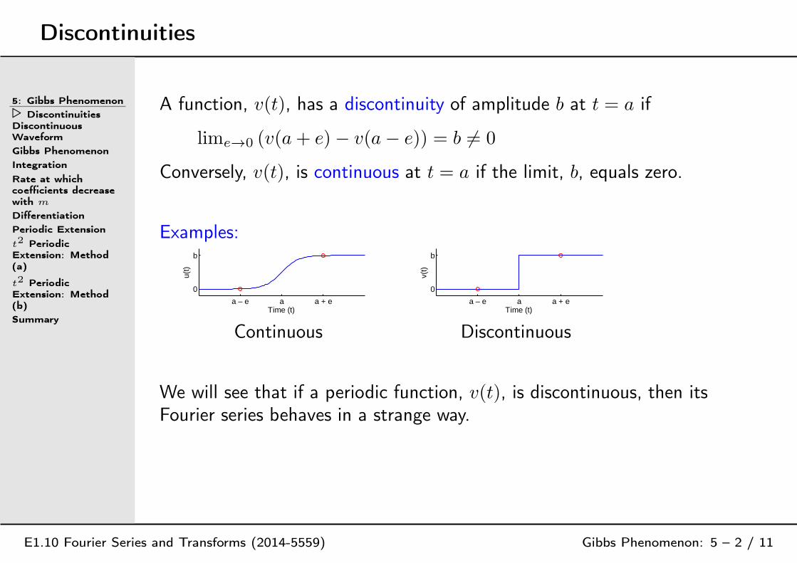
A function, v(t), has a discontinuity of amplitude b at t = a if
lime→0 (v(a+ e)− v(a− e)) = b 6= 0
Conversely, v(t), is continuous at t = a if the limit, b, equals zero.
Examples:
a – e a a + e
0
b
Time (t)
u(t)
a – e a a + e
0
b
Time (t)
v(t)
Continuous Discontinuous
We will see that if a periodic function, v(t), is discontinuous, then itsFourier series behaves in a strange way.

Discontinuous Waveform
5: Gibbs Phenomenon
Discontinuities
⊲DiscontinuousWaveform
Gibbs Phenomenon
Integration
Rate at whichcoefficients decreasewith m
Differentiation
Periodic Extension
t2 PeriodicExtension: Method(a)
t2 PeriodicExtension: Method(b)
Summary
E1.10 Fourier Series and Transforms (2014-5559) Gibbs Phenomenon: 5 – 3 / 11
Pulse: T = 1F
= 20, width=12T , height A = 1
Um = 1T
∫ 0.5T
0Ae−i2πmFtdt
= i
2πmFT
[
e−i2πmFt]0.5T
0
= i
2πm
(
e−iπm − 1)
= ((−1)m−1)i2πm
=
0 m 6= 0, even
0.5 m = 0−i
mπm odd
So, u(t) = 12 + 2
π
(
sin 2πFt+ 13 sin 6πFt
+ 15 sin 10πFt+ . . .
)
Define: uN (t) =∑N
m=−NUmei2πmFt
uN (0) = 0.5 ∀N
maxt uN (t) −→N→∞
12 + 1
π
∫ π
0sin t
tdt≈ 1.0895
0 5 10 15 20
0
0.5
1
0 5 10 15 20
0
0.5
1 max(u0)=0.500
N=0
0 5 10 15 20
0
0.5
1 max(u1)=1.137
N=1
0 5 10 15 20
0
0.5
1 max(u3)=1.100
N=3
0 5 10 15 20
0
0.5
1 max(u5)=1.094
N=5
0 5 10 15 20
0
0.5
1 max(u41
)=1.089
N=41
-1 -0.5 0 0.5 1
0
0.5
1 max(u41
)=1.089
[Enlarged View: u41(t)]

[Powers of −1 and i]
E1.10 Fourier Series and Transforms (2014-5559) Gibbs Phenomenon: 5 – note 1 of slide 3
Expressions involving (−1)m or, less commonly, im arise quite frequently and it is worth becoming
familiar with them. They can arise in several guises:
e−iπm = eiπm =(
eiπ)m
= cos (πm) = (−1)m
ei12πm =
(
ei12π)m
= im
e−i 12πm =
(
e−i 12π)m
= (−i)m
As m increases these expressions repeat with periods of 2 or 4. Simple expressions involving these
quantities make useful sequences.
m −4 −3 −2 −1 0 1 2 3 4
(−1)m = cosπm = eiπm 1 −1 1 −1 1 −1 1 −1 1
im = ei0.5πm 1 i −1 −i 1 i −1 −i 1
(−i)m = e−i0.5πm 1 −i −1 i 1 −i −1 i 112(1 + (−1)m) 1 0 1 0 1 0 1 0 1
12(1− (−1)m) 0 1 0 1 0 1 0 1 0
12(im + (−i)m) = cos 0.5πm 1 0 −1 0 1 0 −1 0 1
14(1 + (−1)m + im + (−i)m) 1 0 0 0 1 0 0 0 1
Gibbs Phenomenon
5: Gibbs Phenomenon
DiscontinuitiesDiscontinuousWaveform
⊲ Gibbs Phenomenon
Integration
Rate at whichcoefficients decreasewith m
Differentiation
Periodic Extension
t2 PeriodicExtension: Method(a)
t2 PeriodicExtension: Method(b)
Summary
E1.10 Fourier Series and Transforms (2014-5559) Gibbs Phenomenon: 5 – 4 / 11
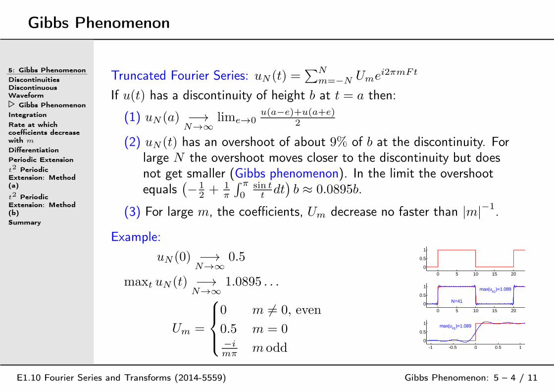
Truncated Fourier Series: uN (t) =∑N
m=−NUmei2πmFt
If u(t) has a discontinuity of height b at t = a then:
(1) uN (a) −→N→∞
lime→0u(a−e)+u(a+e)
2
(2) uN (t) has an overshoot of about 9% of b at the discontinuity. Forlarge N the overshoot moves closer to the discontinuity but doesnot get smaller (Gibbs phenomenon). In the limit the overshootequals
(
− 12 + 1
π
∫ π
0sin t
tdt)
b ≈ 0.0895b.
(3) For large m, the coefficients, Um decrease no faster than |m|−1
.
Example:
uN (0) −→N→∞
0.5
maxt uN (t) −→N→∞
1.0895 . . .
Um =
0 m 6= 0, even
0.5 m = 0−i
mπm odd
0 5 10 15 20
0
0.5
1
0 5 10 15 20
0
0.5
1 max(u41
)=1.089
N=41
-1 -0.5 0 0.5 1
0
0.5
1 max(u41
)=1.089

[Origin of Gibbs Phenomenon]
E1.10 Fourier Series and Transforms (2014-5559) Gibbs Phenomenon: 5 – note 1 of slide 4
This topic is included for interest but is not examinable.
Our first goal is to express the partial Fourier series, uN (t), in terms of the original signal, u(t). We
begin by substituting the integral expression for Un in the partial Fourier series
uN (t) =∑+N
n=−NUne
i2πnFt=∑+N
n=−N
(
1T
∫ T
0 u(τ)e−i2πnFτdτ)
ei2πnFt
Now we swap the order of the integration and the finite summation (OK if the integral converges ∀n)
uN (t) = 1T
∫ T
0 u(τ)(
∑+Nn=−N
ei2πnF (t−τ))
dτ
Now apply the formula for the sum of a geometric progression with z = ei2πF (t−τ):∑+N
n=−Nzn = z−N
−zN+1
1−z= z−(N+0.5)
−zN+0.5
z−0.5−z0.5
uN (t) = 1T
∫ T
0 u(τ) ei2π(N+0.5)F(τ−t)
−e−i2π(N+0.5)F(τ−t)
ei2π0.5F(τ−t)−e−i2π0.5F(τ−t) dτ
= 1T
∫ T
0 u(τ)sinπ(2N+1)F (τ−t)
sinπF (τ−t)dτ
So if we define the Dirichlet Kernel to be DN (x) =sin((N+0.5)x)
sin 0.5x, and set x = 2πF (τ − t), we obtain
uN (t) = 1T
∫ T
0 u(τ)DN (2πF (τ − t)) dτ
So what we have shown is that uN (t) can be obtained by multiplying u(τ) by a time-shifted DirichletKernel and then integrating over one period. Next we will look at the properties of the Dirichlet Kernel.
[Dirichlet Kernel]
E1.10 Fourier Series and Transforms (2014-5559) Gibbs Phenomenon: 5 – note 2 of slide 4
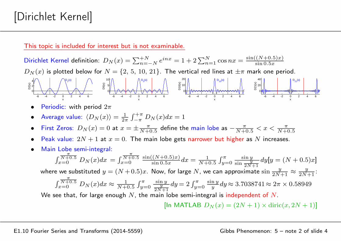
This topic is included for interest but is not examinable.
Dirichlet Kernel definition: DN (x) =∑+N
n=−Neinx = 1 + 2
∑Nn=1 cosnx =
sin((N+0.5)x)sin 0.5x
DN (x) is plotted below for N = 2, 5, 10, 21. The vertical red lines at ±π mark one period.
-6 -4 -2 0 2 4 6
0
2
4 D2(x)
x
D2(
x)
-6 -4 -2 0 2 4 6
0
5
10 D5(x)
x
D5(
x)
-6 -4 -2 0 2 4 6
0
10
20 D10
(x)
x
D10
(x)
-6 -4 -2 0 2 4 6
0
20
40 D21
(x)
x
D21
(x)
• Periodic: with period 2π
• Average value: 〈DN (x)〉 = 12π
∫+π
−πDN (x)dx = 1
• First Zeros: DN (x) = 0 at x = ± πN+0.5
define the main lobe as − πN+0.5
< x < πN+0.5
• Peak value: 2N + 1 at x = 0. The main lobe gets narrower but higher as N increases.
• Main Lobe semi-integral:∫
πN+0.5x=0 DN (x)dx =
∫
πN+0.5x=0
sin((N+0.5)x)sin 0.5x
dx = 1N+0.5
∫ π
y=0sin y
sin y2N+1
dy[y = (N + 0.5)x]
where we substituted y = (N +0.5)x. Now, for large N , we can approximate sin y
2N+1≈ y
2N+1:
∫
πN+0.5x=0 DN (x)dx ≈ 1
N+0.5
∫ π
y=0sin y
y2N+1
dy= 2∫ π
y=0sin y
ydy≈ 3.7038741≈ 2π × 0.58949
We see that, for large enough N , the main lobe semi-integral is independent of N .
[In MATLAB DN (x) = (2N + 1)× diric(x, 2N + 1)]
[Gibbs Phenomenon Overshoot]
E1.10 Fourier Series and Transforms (2014-5559) Gibbs Phenomenon: 5 – note 3 of slide 4
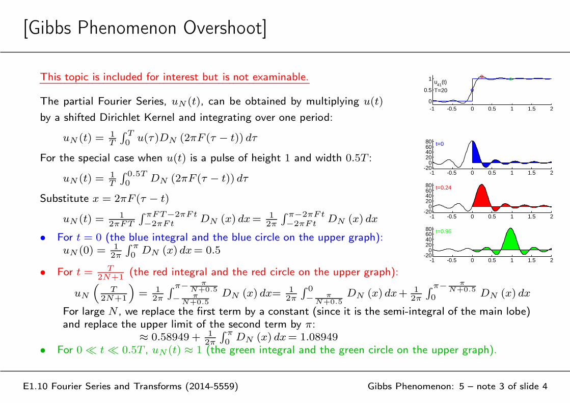
This topic is included for interest but is not examinable.
The partial Fourier Series, uN (t), can be obtained by multiplying u(t)
by a shifted Dirichlet Kernel and integrating over one period:
uN (t) = 1T
∫ T
0 u(τ)DN (2πF (τ − t)) dτ
For the special case when u(t) is a pulse of height 1 and width 0.5T :
uN (t) = 1T
∫ 0.5T0 DN (2πF (τ − t)) dτ
Substitute x = 2πF (τ − t)
uN (t) = 12πFT
∫ πFT−2πFt
−2πFtDN (x) dx= 1
2π
∫ π−2πFt
−2πFtDN (x) dx
• For t = 0 (the blue integral and the blue circle on the upper graph):uN (0) = 1
2π
∫ π
0 DN (x) dx= 0.5
-1 -0.5 0 0.5 1 1.5 20
0.5
1 u41
(t)
T=20
-1 -0.5 0 0.5 1 1.5 2-20
020406080 t=0
-1 -0.5 0 0.5 1 1.5 2-20
020406080 t=0.24
-1 -0.5 0 0.5 1 1.5 2-20
020406080 t=0.96
• For t = T2N+1
(the red integral and the red circle on the upper graph):
uN
(
T2N+1
)
= 12π
∫ π−
πN+0.5
−
πN+0.5
DN (x) dx= 12π
∫ 0−
πN+0.5
DN (x) dx+ 12π
∫ π−
πN+0.5
0 DN (x) dx
For large N , we replace the first term by a constant (since it is the semi-integral of the main lobe)and replace the upper limit of the second term by π:
≈ 0.58949 + 12π
∫ π
0 DN (x) dx= 1.08949• For 0 ≪ t ≪ 0.5T , uN (t) ≈ 1 (the green integral and the green circle on the upper graph).
Integration
5: Gibbs Phenomenon
DiscontinuitiesDiscontinuousWaveform
Gibbs Phenomenon
⊲ Integration
Rate at whichcoefficients decreasewith m
Differentiation
Periodic Extension
t2 PeriodicExtension: Method(a)
t2 PeriodicExtension: Method(b)
Summary
E1.10 Fourier Series and Transforms (2014-5559) Gibbs Phenomenon: 5 – 5 / 11
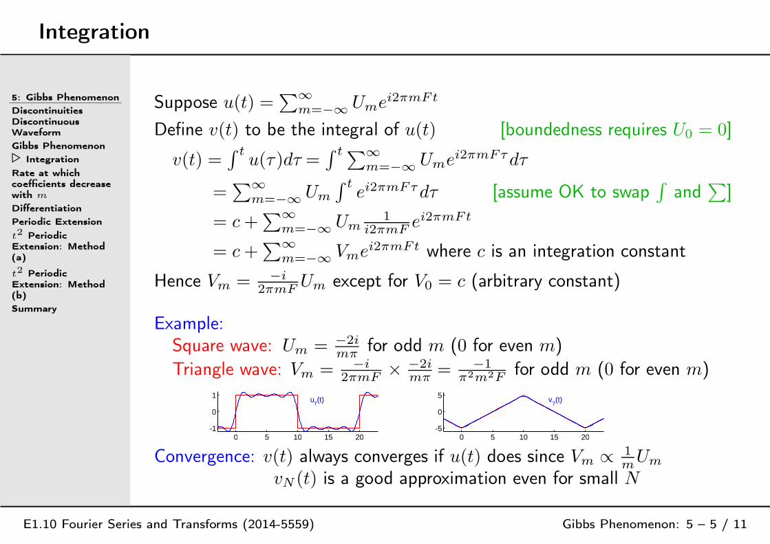
Suppose u(t) =∑∞
m=−∞ Umei2πmFt
Define v(t) to be the integral of u(t) [boundedness requires U0 = 0]
v(t) =∫ t
u(τ )dτ =∫ t ∑∞
m=−∞ Umei2πmFτdτ
=∑∞
m=−∞ Um
∫ tei2πmFτdτ [assume OK to swap
∫
and∑
]
= c+∑∞
m=−∞ Um1
i2πmFei2πmFt
= c+∑∞
m=−∞ Vmei2πmFt where c is an integration constant
Hence Vm = −i
2πmFUm except for V0 = c (arbitrary constant)
Example:Square wave: Um = −2i
mπfor odd m (0 for even m)
Triangle wave: Vm = −i
2πmF× −2i
mπ= −1
π2m2Ffor odd m (0 for even m)
0 5 10 15 20-1
0
1 u7(t)
0 5 10 15 20-5
0
5 v7(t)
Convergence: v(t) always converges if u(t) does since Vm ∝ 1mUm
vN (t) is a good approximation even for small N
Rate at which coefficients decrease with m
5: Gibbs Phenomenon
DiscontinuitiesDiscontinuousWaveform
Gibbs Phenomenon
Integration
⊲
Rate at whichcoefficientsdecrease with m
Differentiation
Periodic Extension
t2 PeriodicExtension: Method(a)
t2 PeriodicExtension: Method(b)
Summary
E1.10 Fourier Series and Transforms (2014-5559) Gibbs Phenomenon: 5 – 6 / 11
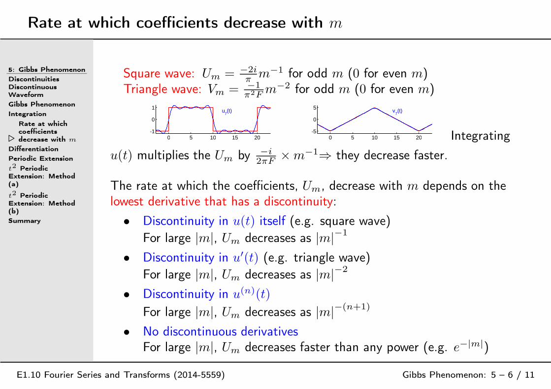
Square wave: Um = −2iπ
m−1 for odd m (0 for even m)Triangle wave: Vm = −1
π2Fm−2 for odd m (0 for even m)
0 5 10 15 20-1
0
1 u7(t)
0 5 10 15 20-5
0
5 v7(t)
Integrating
u(t) multiplies the Um by −i
2πF ×m−1⇒ they decrease faster.
The rate at which the coefficients, Um, decrease with m depends on thelowest derivative that has a discontinuity:
• Discontinuity in u(t) itself (e.g. square wave)
For large |m|, Um decreases as |m|−1
• Discontinuity in u′(t) (e.g. triangle wave)
For large |m|, Um decreases as |m|−2
• Discontinuity in u(n)(t)
For large |m|, Um decreases as |m|−(n+1)
• No discontinuous derivativesFor large |m|, Um decreases faster than any power (e.g. e−|m|)
Differentiation
5: Gibbs Phenomenon
DiscontinuitiesDiscontinuousWaveform
Gibbs Phenomenon
Integration
Rate at whichcoefficients decreasewith m
⊲ Differentiation
Periodic Extension
t2 PeriodicExtension: Method(a)
t2 PeriodicExtension: Method(b)
Summary
E1.10 Fourier Series and Transforms (2014-5559) Gibbs Phenomenon: 5 – 7 / 11
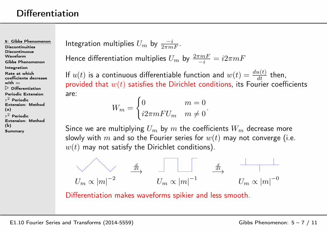
Integration multiplies Um by −i
2πmF.
Hence differentiation multiplies Um by 2πmF
−i= i2πmF
If u(t) is a continuous differentiable function and w(t) = du(t)dt
then,provided that w(t) satisfies the Dirichlet conditions, its Fourier coefficientsare:
Wm =
0 m = 0
i2πmFUm m 6= 0.
Since we are multiplying Um by m the coefficients Wm decrease moreslowly with m and so the Fourier series for w(t) may not converge (i.e.w(t) may not satisfy the Dirichlet conditions).
ddt−→
ddt−→
Um ∝ |m|−2
Um ∝ |m|−1
Um ∝ |m|−0
Differentiation makes waveforms spikier and less smooth.
Periodic Extension
5: Gibbs Phenomenon
DiscontinuitiesDiscontinuousWaveform
Gibbs Phenomenon
Integration
Rate at whichcoefficients decreasewith m
Differentiation
⊲ Periodic Extension
t2 PeriodicExtension: Method(a)
t2 PeriodicExtension: Method(b)
Summary
E1.10 Fourier Series and Transforms (2014-5559) Gibbs Phenomenon: 5 – 8 / 11
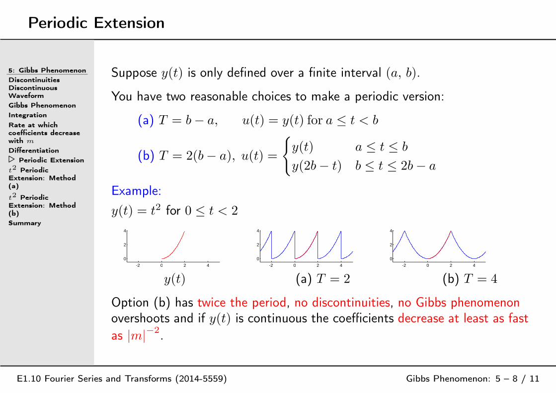
Suppose y(t) is only defined over a finite interval (a, b).
You have two reasonable choices to make a periodic version:
(a) T = b− a, u(t) = y(t) for a ≤ t < b
(b) T = 2(b− a), u(t) =
y(t) a ≤ t ≤ b
y(2b− t) b ≤ t ≤ 2b− a
Example:
y(t) = t2 for 0 ≤ t < 2
-2 0 2 4
0
2
4
-2 0 2 4
0
2
4
-2 0 2 4
0
2
4
y(t) (a) T = 2 (b) T = 4
Option (b) has twice the period, no discontinuities, no Gibbs phenomenonovershoots and if y(t) is continuous the coefficients decrease at least as fast
as |m|−2
.

t2 Periodic Extension: Method (a)
5: Gibbs Phenomenon
DiscontinuitiesDiscontinuousWaveform
Gibbs Phenomenon
Integration
Rate at whichcoefficients decreasewith m
Differentiation
Periodic Extension
⊲
t2 PeriodicExtension: Method(a)
t2 PeriodicExtension: Method(b)
Summary
E1.10 Fourier Series and Transforms (2014-5559) Gibbs Phenomenon: 5 – 9 / 11
y(t) = t2 for 0 ≤ t < 2
Method (a): T = 1F
= 2
Um = 1T
∫ T
0t2e−i2πmFtdt U0 = 1
T
∫ T
0t2dt = 4
3
= 1T
[
t2e−i2πmFt
−i2πmF− 2te−i2πmFt
(−i2πmF )2+ 2e−i2πmFt
(−i2πmF )3
]T
0
Substitute e−i2πmF0 = e−i2πmFT = 1 [for integer m]
= 1T
[
T2
−i2πmF− 2T
(−i2πmF )2
]
= 2iπm
+ 2π2m2
-2 0 2 4
0
2
4 K=1
-2 0 2 4
0
2
4 K=3
-2 0 2 4
0
2
4 K=6
U0:3 = [1.333, 0.203 + 0.637i, 0.051 + 0.318i, 0.023 + 0.212i]
t2 Periodic Extension: Method (b)
5: Gibbs Phenomenon
DiscontinuitiesDiscontinuousWaveform
Gibbs Phenomenon
Integration
Rate at whichcoefficients decreasewith m
Differentiation
Periodic Extension
t2 PeriodicExtension: Method(a)
⊲
t2 PeriodicExtension: Method(b)
Summary
E1.10 Fourier Series and Transforms (2014-5559) Gibbs Phenomenon: 5 – 10 / 11
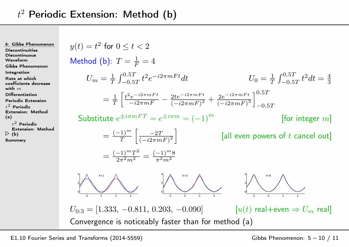
y(t) = t2 for 0 ≤ t < 2
Method (b): T = 1F
= 4
Um = 1T
∫ 0.5T
−0.5Tt2e−i2πmFtdt U0 = 1
T
∫ 0.5T
−0.5Tt2dt = 4
3
= 1T
[
t2e−i2πmFt
−i2πmF− 2te−i2πmFt
(−i2πmF )2+ 2e−i2πmFt
(−i2πmF )3
]0.5T
−0.5T
Substitute e±iπmFT = e±iπm = (−1)m
[for integer m]
= (−1)m
T
[
−2T(−i2πmF )2
]
[all even powers of t cancel out]
= (−1)mT2
2π2m2 = (−1)m8π2m2
-2 0 2 4
0
2
4 K=1
-2 0 2 4
0
2
4 K=3
-2 0 2 4
0
2
4 K=6
U0:3 = [1.333, −0.811, 0.203, −0.090] [u(t) real+even ⇒ Um real]
Convergence is noticeably faster than for method (a)
Summary
5: Gibbs Phenomenon
DiscontinuitiesDiscontinuousWaveform
Gibbs Phenomenon
Integration
Rate at whichcoefficients decreasewith m
Differentiation
Periodic Extension
t2 PeriodicExtension: Method(a)
t2 PeriodicExtension: Method(b)
⊲ Summary
E1.10 Fourier Series and Transforms (2014-5559) Gibbs Phenomenon: 5 – 11 / 11
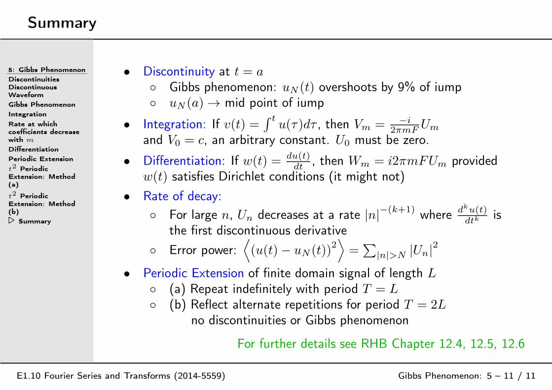
• Discontinuity at t = a
Gibbs phenomenon: uN (t) overshoots by 9% of iump uN (a) → mid point of iump
• Integration: If v(t) =∫ t
u(τ )dτ , then Vm = −i
2πmFUm
and V0 = c, an arbitrary constant. U0 must be zero.
• Differentiation: If w(t) = du(t)dt
, then Wm = i2πmFUm providedw(t) satisfies Dirichlet conditions (it might not)
• Rate of decay:
For large n, Un decreases at a rate |n|−(k+1)
where dku(t)dtk
isthe first discontinuous derivative
Error power:⟨
(u(t)− uN (t))2⟩
=∑
|n|>N|Un|
2
• Periodic Extension of finite domain signal of length L
(a) Repeat indefinitely with period T = L
(b) Reflect alternate repetitions for period T = 2Lno discontinuities or Gibbs phenomenon
For further details see RHB Chapter 12.4, 12.5, 12.6
6: Fourier Transform
⊲6: FourierTransform
Fourier Series asT → ∞
Fourier TransformFourier TransformExamples
Dirac Delta FunctionDirac Delta Function:Scaling andTranslationDirac Delta Function:Products andIntegrals
Periodic Signals
Duality
Time Shifting andScaling
Gaussian Pulse
Summary
E1.10 Fourier Series and Transforms (2014-5559) Fourier Transform: 6 – 1 / 12
Fourier Series as T → ∞
6: Fourier Transform
⊲Fourier Series asT → ∞
Fourier TransformFourier TransformExamples
Dirac Delta FunctionDirac Delta Function:Scaling andTranslationDirac Delta Function:Products andIntegrals
Periodic Signals
Duality
Time Shifting andScaling
Gaussian Pulse
Summary
E1.10 Fourier Series and Transforms (2014-5559) Fourier Transform: 6 – 2 / 12
Fourier Series: u(t) =∑∞
n=−∞ Unei2πnFt
The harmonic frequencies are nF ∀n and are spaced F = 1T
apart.
As T gets larger, the harmonic spacing becomes smaller.e.g. T = 1 s ⇒ F = 1Hz
T = 1day ⇒ F = 11.57µHz
If T → ∞ then the harmonic spacing becomes zero, the sum becomes anintegral and we get the Fourier Transform:
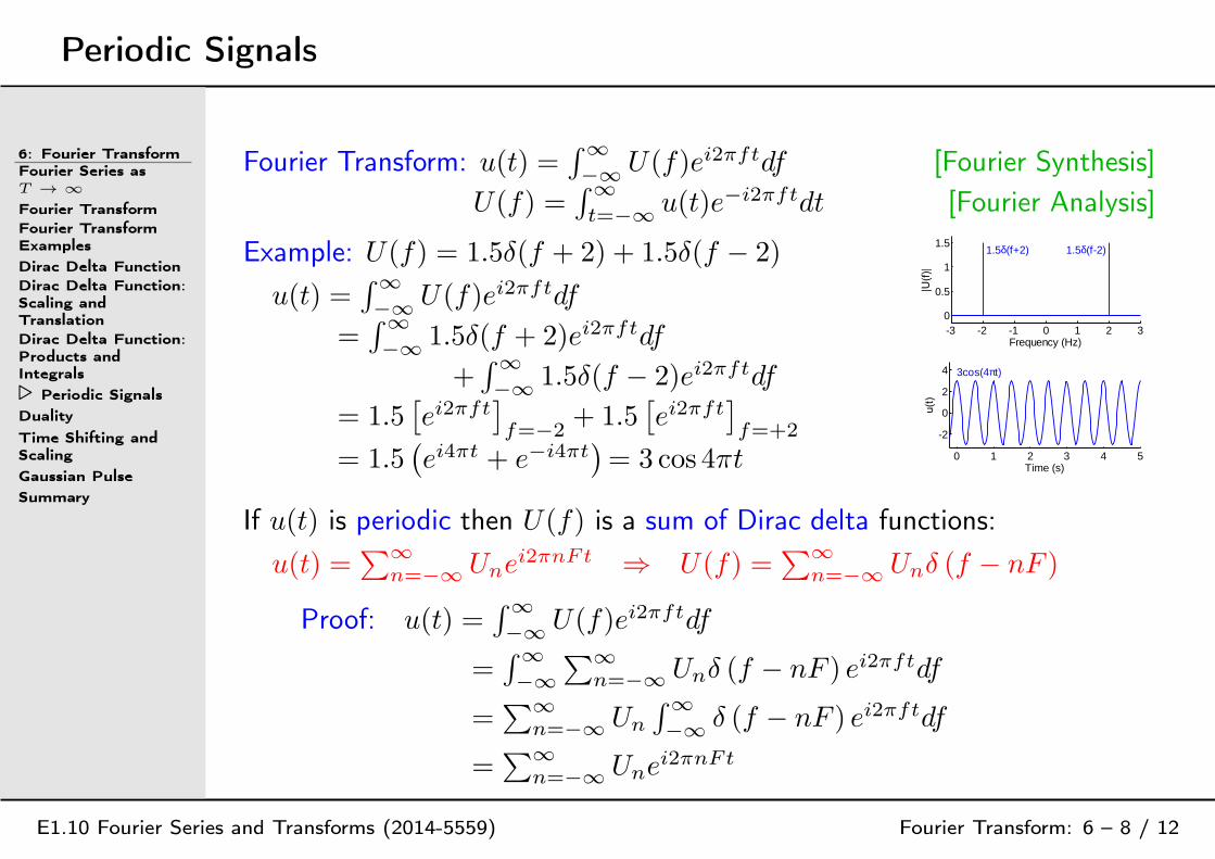
u(t) =∫ +∞f=−∞ U(f)ei2πftdf
Here, U(f), is the spectral density of u(t).
• U(f) is a continuous function of f .• U(f) is complex-valued.• u(t) real ⇒ U(f) is conjugate symmetric ⇔ U(−f) = U(f)∗.• Units: if u(t) is in volts, then U(f)df must also be in volts
⇒ U(f) is in volts/Hz (hence “spectral density”).
Fourier Transform
6: Fourier TransformFourier Series asT → ∞
⊲ Fourier TransformFourier TransformExamples
Dirac Delta FunctionDirac Delta Function:Scaling andTranslationDirac Delta Function:Products andIntegrals
Periodic Signals
Duality
Time Shifting andScaling
Gaussian Pulse
Summary
E1.10 Fourier Series and Transforms (2014-5559) Fourier Transform: 6 – 3 / 12
Fourier Series: u(t) =∑∞
n=−∞ Unei2πnFt
The summation is over a set of equally spaced frequenciesfn = nF where the spacing between them is ∆f = F = 1
T.
Un =⟨
u(t)e−i2πnFt⟩
= ∆f∫ 0.5T
t=−0.5Tu(t)e−i2πnFtdt
Spectral Density: If u(t) has finite energy, Un → 0 as ∆f → 0. So wedefine a spectral density, U(fn) =
Un
∆f, on the set of frequencies fn:
U(fn) =Un
∆f=
∫ 0.5T
t=−0.5Tu(t)e−i2πfntdt
we can write [Substitute Un = U(fn)∆f ]u(t) =
∑∞n=−∞ U(fn)e
i2πfnt∆f
Fourier Transform: Now if we take the limit as ∆f → 0, we get
u(t) =∫∞−∞ U(f)ei2πftdf [Fourier Synthesis]
U(f) =∫∞t=−∞ u(t)e−i2πftdt [Fourier Analysis]
For non-periodic signals Un → 0 as ∆f → 0 and U(fn) =Un
∆fremains
finite. However, if u(t) contains an exactly periodic component, then thecorresponding U(fn) will become infinite as ∆f → 0. We will deal with it.
Fourier Transform Examples
6: Fourier TransformFourier Series asT → ∞
Fourier Transform
⊲Fourier TransformExamples
Dirac Delta FunctionDirac Delta Function:Scaling andTranslationDirac Delta Function:Products andIntegrals
Periodic Signals
Duality
Time Shifting andScaling
Gaussian Pulse
Summary
E1.10 Fourier Series and Transforms (2014-5559) Fourier Transform: 6 – 4 / 12
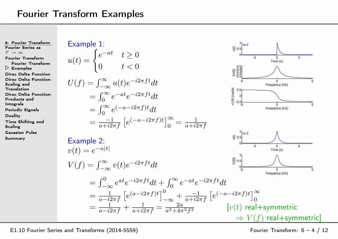
Example 1:
u(t) =
e−at t ≥ 0
0 t < 0
U(f) =∫∞−∞ u(t)e−i2πftdt
=∫∞0
e−ate−i2πftdt
=∫∞0
e(−a−i2πf)tdt
-5 0 50
0.5
1
Time (s)
u(t)
a=2
-5 0 50.10.20.30.40.5
Frequency (Hz)
|U(f
)|
-5 0 5-0.5
0
0.5
Frequence (Hz)
<U
(f)
(rad
/pi)
= −1a+i2πf
[
e(−a−i2πf)t]∞0
= 1a+i2πf
Example 2:v(t) = e−a|t|
V (f) =∫∞−∞ v(t)e−i2πftdt
-5 0 50
0.5
1
Time (s)
v(t)
a=2
-5 0 50
0.5
1
Frequency (Hz)
|V(f
)|
=∫ 0
−∞ eate−i2πftdt+∫∞0
e−ate−i2πftdt
= 1a−i2πf
[
e(a−i2πf)t]0
−∞ + −1a+i2πf
[
e(−a−i2πf)t]∞0
= 1a−i2πf + 1
a+i2πf = 2aa2+4π2f2 [v(t) real+symmetric
⇒ V (f) real+symmetric]
Dirac Delta Function
6: Fourier TransformFourier Series asT → ∞
Fourier TransformFourier TransformExamples
⊲Dirac DeltaFunction
Dirac Delta Function:Scaling andTranslationDirac Delta Function:Products andIntegrals
Periodic Signals
Duality
Time Shifting andScaling
Gaussian Pulse
Summary
E1.10 Fourier Series and Transforms (2014-5559) Fourier Transform: 6 – 5 / 12
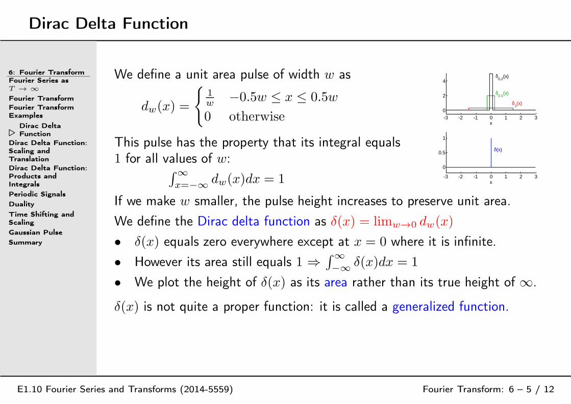
We define a unit area pulse of width w as
dw(x) =
1w
−0.5w ≤ x ≤ 0.5w
0 otherwise
This pulse has the property that its integral equals1 for all values of w:
∫∞x=−∞ dw(x)dx = 1
-3 -2 -1 0 1 2 30
2
4
δ3(x)
δ0.5
(x)
δ0.2
(x)
x
-3 -2 -1 0 1 2 3
0
0.5
1
δ(x)
x
If we make w smaller, the pulse height increases to preserve unit area.
We define the Dirac delta function as δ(x) = limw→0 dw(x)
• δ(x) equals zero everywhere except at x = 0 where it is infinite.
• However its area still equals 1 ⇒∫∞−∞ δ(x)dx = 1
• We plot the height of δ(x) as its area rather than its true height of ∞.
δ(x) is not quite a proper function: it is called a generalized function.
Dirac Delta Function: Scaling and Translation
6: Fourier TransformFourier Series asT → ∞
Fourier TransformFourier TransformExamples
Dirac Delta Function
⊲
Dirac DeltaFunction: Scalingand Translation
Dirac Delta Function:Products andIntegrals
Periodic Signals
Duality
Time Shifting andScaling
Gaussian Pulse
Summary
E1.10 Fourier Series and Transforms (2014-5559) Fourier Transform: 6 – 6 / 12
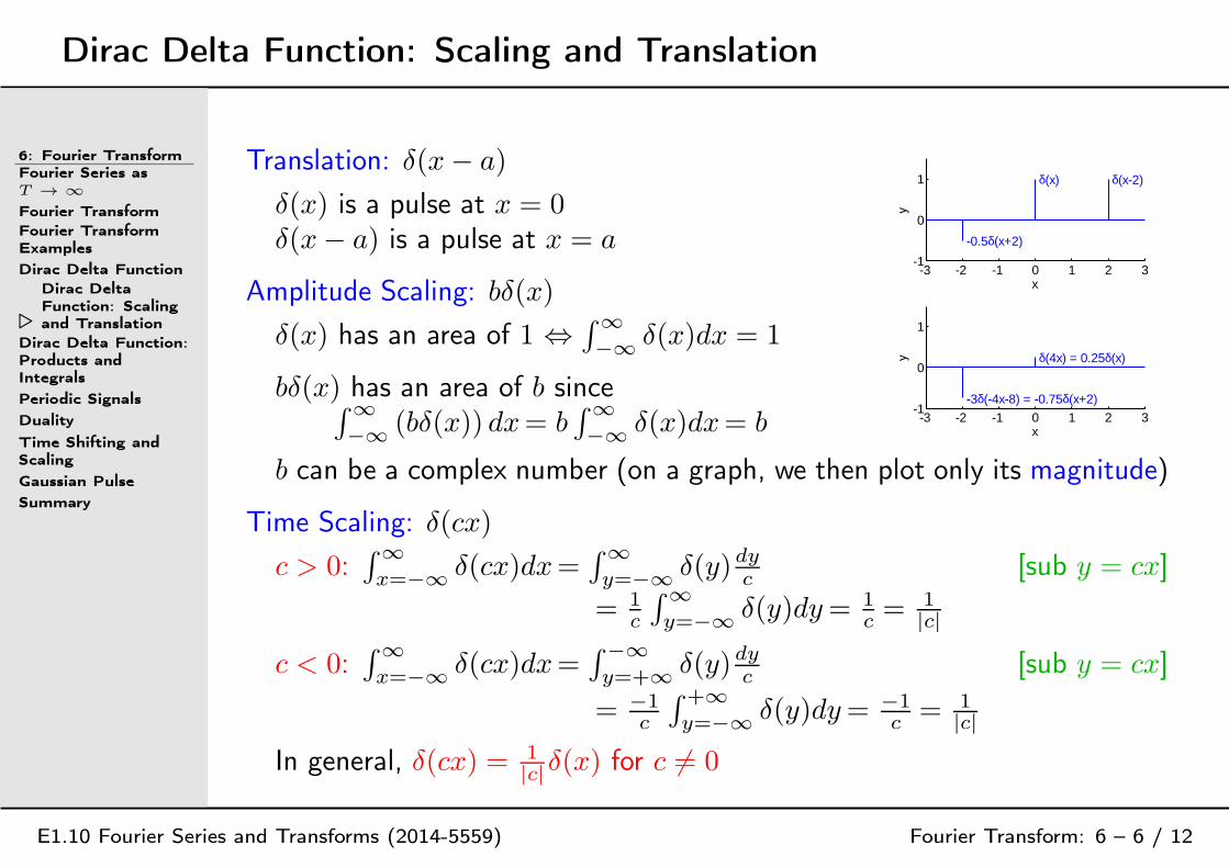
Translation: δ(x− a)
δ(x) is a pulse at x = 0δ(x− a) is a pulse at x = a
Amplitude Scaling: bδ(x)
δ(x) has an area of 1 ⇔∫∞−∞ δ(x)dx = 1
bδ(x) has an area of b since∫∞−∞ (bδ(x)) dx= b
∫∞−∞ δ(x)dx= b
-3 -2 -1 0 1 2 3-1
0
1 δ(x) δ(x-2)
-0.5δ(x+2)
x
-3 -2 -1 0 1 2 3-1
0
1
δ(4x) = 0.25δ(x)
-3δ(-4x-8) = -0.75δ(x+2)
x
b can be a complex number (on a graph, we then plot only its magnitude)
Time Scaling: δ(cx)
c > 0:∫∞x=−∞ δ(cx)dx=
∫∞y=−∞ δ(y)dy
c[sub y = cx]
= 1c
∫∞y=−∞ δ(y)dy= 1
c= 1
|c|
c < 0:∫∞x=−∞ δ(cx)dx=
∫ −∞y=+∞ δ(y)dy
c[sub y = cx]
= −1c
∫ +∞y=−∞ δ(y)dy= −1
c= 1
|c|
In general, δ(cx) = 1|c|δ(x) for c 6= 0
Dirac Delta Function: Products and Integrals
6: Fourier TransformFourier Series asT → ∞
Fourier TransformFourier TransformExamples
Dirac Delta FunctionDirac Delta Function:Scaling andTranslation
⊲
Dirac DeltaFunction:Products andIntegrals
Periodic Signals
Duality
Time Shifting andScaling
Gaussian Pulse
Summary
E1.10 Fourier Series and Transforms (2014-5559) Fourier Transform: 6 – 7 / 12
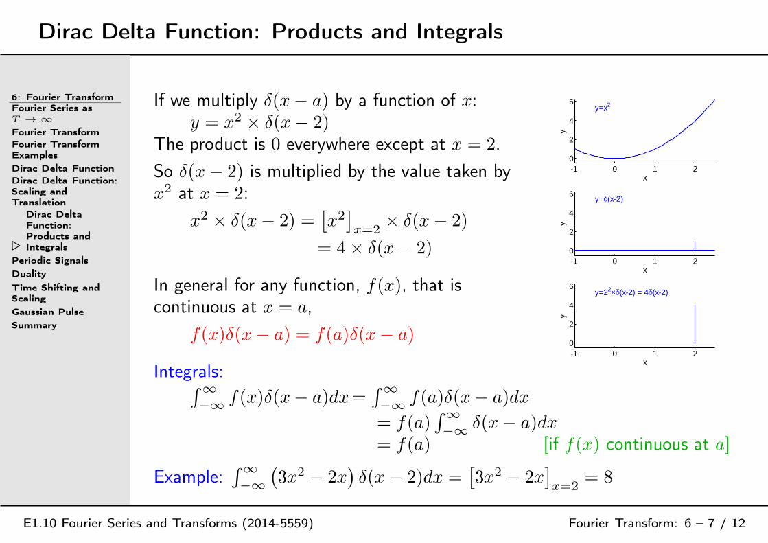
If we multiply δ(x− a) by a function of x:y = x2 × δ(x− 2)
The product is 0 everywhere except at x = 2.
So δ(x− 2) is multiplied by the value taken byx2 at x = 2:
x2 × δ(x− 2) =[
x2]
x=2× δ(x− 2)
= 4× δ(x− 2)
In general for any function, f(x), that iscontinuous at x = a,
f(x)δ(x− a) = f(a)δ(x− a)
Integrals:
-1 0 1 20
2
4
6y=x2
x
-1 0 1 20
2
4
6y=δ(x-2)
x
-1 0 1 20
2
4
6y=22×δ(x-2) = 4δ(x-2)
x
∫∞−∞ f(x)δ(x− a)dx=
∫∞−∞ f(a)δ(x− a)dx
= f(a)∫∞−∞ δ(x− a)dx
= f(a) [if f(x) continuous at a]
Example:∫∞−∞
(
3x2 − 2x)
δ(x− 2)dx =[
3x2 − 2x]
x=2= 8
Periodic Signals
6: Fourier TransformFourier Series asT → ∞
Fourier TransformFourier TransformExamples
Dirac Delta FunctionDirac Delta Function:Scaling andTranslationDirac Delta Function:Products andIntegrals
⊲ Periodic Signals
Duality
Time Shifting andScaling
Gaussian Pulse
Summary
E1.10 Fourier Series and Transforms (2014-5559) Fourier Transform: 6 – 8 / 12
Fourier Transform: u(t) =∫∞−∞ U(f)ei2πftdf [Fourier Synthesis]
U(f) =∫∞t=−∞ u(t)e−i2πftdt [Fourier Analysis]
Example: U(f) = 1.5δ(f + 2) + 1.5δ(f − 2)
u(t) =∫∞−∞ U(f)ei2πftdf
=∫∞−∞ 1.5δ(f + 2)ei2πftdf
+∫∞−∞ 1.5δ(f − 2)ei2πftdf
= 1.5[
ei2πft]
f=−2+ 1.5
[
ei2πft]
f=+2
= 1.5(
ei4πt + e−i4πt)
= 3 cos 4πt
-3 -2 -1 0 1 2 30
0.5
1
1.5 1.5δ(f+2) 1.5δ(f-2)
Frequency (Hz)
0 1 2 3 4 5
-2
0
2
4 3cos(4πt)
Time (s)
If u(t) is periodic then U(f) is a sum of Dirac delta functions:
u(t) =∑∞
n=−∞ Unei2πnFt ⇒ U(f) =
∑∞n=−∞ Unδ (f − nF )
Proof: u(t) =∫∞−∞ U(f)ei2πftdf
=∫∞−∞
∑∞n=−∞ Unδ (f − nF ) ei2πftdf
=∑∞
n=−∞ Un
∫∞−∞ δ (f − nF ) ei2πftdf
=∑∞
n=−∞ Unei2πnFt
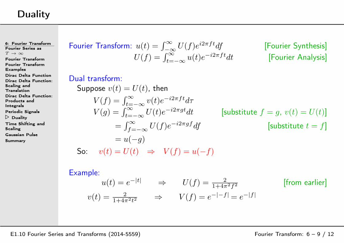
Duality
6: Fourier TransformFourier Series asT → ∞
Fourier TransformFourier TransformExamples
Dirac Delta FunctionDirac Delta Function:Scaling andTranslationDirac Delta Function:Products andIntegrals
Periodic Signals
⊲ Duality
Time Shifting andScaling
Gaussian Pulse
Summary
E1.10 Fourier Series and Transforms (2014-5559) Fourier Transform: 6 – 9 / 12
Fourier Transform: u(t) =∫∞−∞ U(f)ei2πftdf [Fourier Synthesis]
U(f) =∫∞t=−∞ u(t)e−i2πftdt [Fourier Analysis]
Dual transform:Suppose v(t) = U(t), then
V (f) =∫∞t=−∞ v(t)e−i2πftdτ
V (g) =∫∞t=−∞ U(t)e−i2πgtdt [substitute f = g, v(t) = U(t)]
=∫∞f=−∞ U(f)e−i2πgfdf [substitute t = f ]
= u(−g)
So: v(t) = U(t) ⇒ V (f) = u(−f)
Example:u(t) = e−|t| ⇒ U(f) = 2
1+4π2f2 [from earlier]
v(t) = 21+4π2t2
⇒ V (f) = e−|−f | = e−|f |
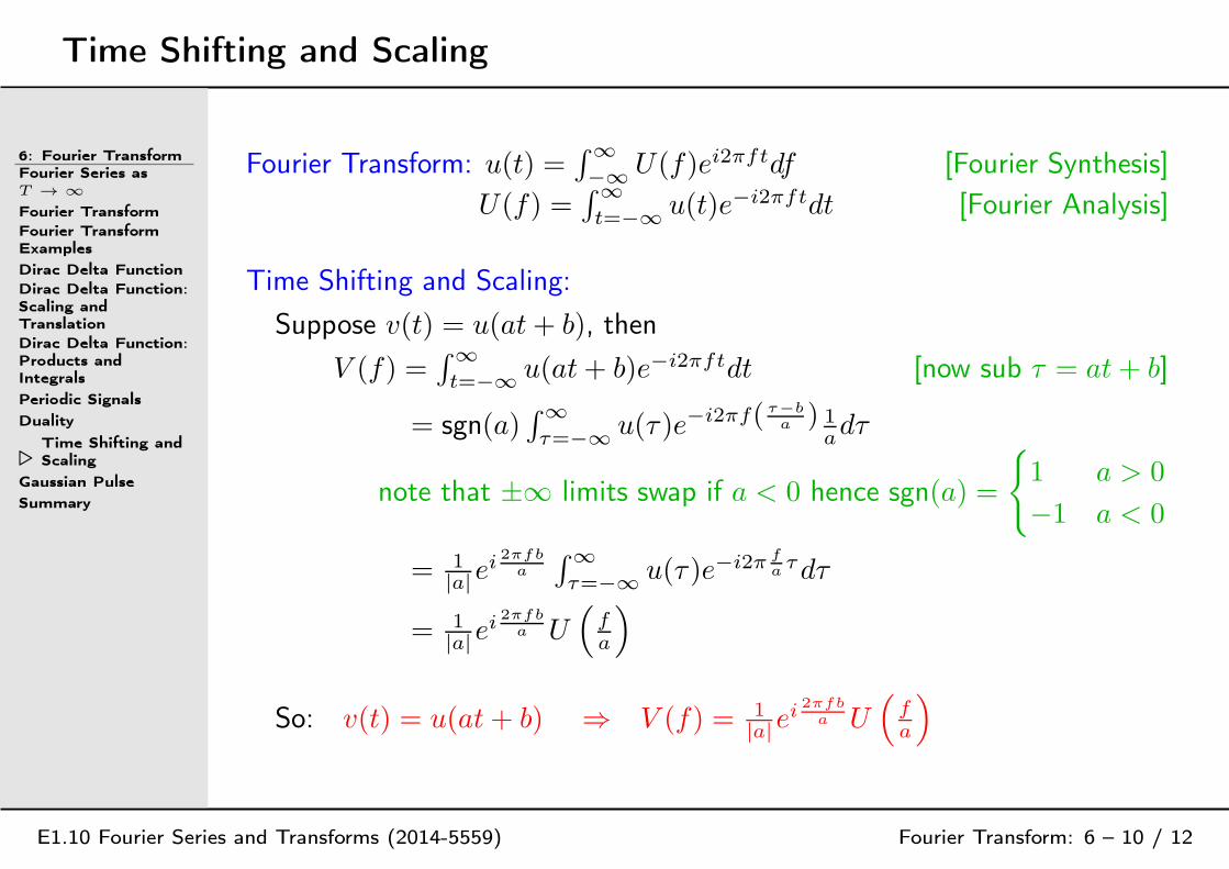
Time Shifting and Scaling
6: Fourier TransformFourier Series asT → ∞
Fourier TransformFourier TransformExamples
Dirac Delta FunctionDirac Delta Function:Scaling andTranslationDirac Delta Function:Products andIntegrals
Periodic Signals
Duality
⊲Time Shifting andScaling
Gaussian Pulse
Summary
E1.10 Fourier Series and Transforms (2014-5559) Fourier Transform: 6 – 10 / 12
Fourier Transform: u(t) =∫∞−∞ U(f)ei2πftdf [Fourier Synthesis]
U(f) =∫∞t=−∞ u(t)e−i2πftdt [Fourier Analysis]
Time Shifting and Scaling:
Suppose v(t) = u(at+ b), then
V (f) =∫∞t=−∞ u(at+ b)e−i2πftdt [now sub τ = at+ b]
= sgn(a)∫∞τ=−∞ u(τ )e−i2πf( τ−b
a ) 1adτ
note that ±∞ limits swap if a < 0 hence sgn(a) =
1 a > 0
−1 a < 0
= 1|a|e
i2πfb
a
∫∞τ=−∞ u(τ )e−i2π f
aτdτ
= 1|a|e
i2πfb
a U(
fa
)
So: v(t) = u(at+ b) ⇒ V (f) = 1|a|e
i2πfb
a U(
fa
)

Gaussian Pulse
6: Fourier TransformFourier Series asT → ∞
Fourier TransformFourier TransformExamples
Dirac Delta FunctionDirac Delta Function:Scaling andTranslationDirac Delta Function:Products andIntegrals
Periodic Signals
Duality
Time Shifting andScaling
⊲ Gaussian Pulse
Summary
E1.10 Fourier Series and Transforms (2014-5559) Fourier Transform: 6 – 11 / 12
Gaussian Pulse: u(t) = 1√2πσ2
e−t2
2σ2
This is a Normal (or Gaussian) probability distribution, so∫∞−∞ u(t)dt = 1.
U(f) =∫∞−∞ u(t)e−i2πftdt= 1√
2πσ2
∫∞−∞ e−
t2
2σ2 e−i2πftdt
= 1√2πσ2
∫∞−∞ e−
1
2σ2 (t2+i4πσ2ft)dt
= 1√2πσ2
∫∞−∞ e
− 1
2σ2
(
t2+i4πσ2ft+(i2πσ2f)2−(i2πσ2f)2)
dt
= e1
2σ2 (i2πσ2f)2 1√2πσ2
∫∞−∞ e−
1
2σ2 (t+i2πσ2f)2dt
(i)= e
1
2σ2 (i2πσ2f)2 = e−1
2(2πσf)2
[(i) uses a result from complex analysis theory that:1√
2πσ2
∫∞−∞ e−
1
2σ2 (t+i2πσ2f)2dt = 1√2πσ2
∫∞−∞ e−
1
2σ2t2dt = 1]
-4 -2 0 2 40
0.2
0.4 σ=1
Time (s)
u(t)
-0.6 -0.4 -0.2 0 0.2 0.4 0.60
0.5
1 1/(2πσ)=0.159
Frequency (Hz)
|U(f
)|
Uniquely, the Fourier Transform of a Gaussian pulse is a Gaussian pulse.

Summary
6: Fourier TransformFourier Series asT → ∞
Fourier TransformFourier TransformExamples
Dirac Delta FunctionDirac Delta Function:Scaling andTranslationDirac Delta Function:Products andIntegrals
Periodic Signals
Duality
Time Shifting andScaling
Gaussian Pulse
⊲ Summary
E1.10 Fourier Series and Transforms (2014-5559) Fourier Transform: 6 – 12 / 12
• Fourier Transform: Inverse transform (synthesis): u(t) =
∫∞−∞ U(f)ei2πftdf
Forward transform (analysis): U(f) =∫∞t=−∞ u(t)e−i2πftdt
⊲ U(f) is the spectral density function (e.g. Volts/Hz)
• Dirac Delta Function: δ(t) is a zero-width infinite-height pulse with
∫∞−∞ δ(t)dt = 1
Integral:∫∞−∞ f(t)δ(t− a) = f(a)
Scaling: δ(ct) = 1|c|δ(t)
• Periodic Signals: u(t) =∑∞
n=−∞ Unei2πnFt
⇒ U(f) =∑∞
n=−∞ Unδ (f − nF )• Fourier Transform Properties:
v(t) = U(t) ⇒ V (f) = u(−f)
v(t) = u(at+ b) ⇒ V (f) = 1|a|e
i2πfb
a U(
fa
)
v(t) = 1√2πσ2
e−1
2( t
σ )2
⇒ V (f) = e−1
2(2πσf)2
For further details see RHB Chapter 13.1 (uses ω instead of f)
7: Fourier Transforms: Convolution and
Parseval’s Theorem
⊲
7: FourierTransforms:Convolution andParseval’sTheorem
Multiplication ofSignals
MultiplicationExample
Convolution Theorem
Convolution Example
ConvolutionProperties
Parseval’s Theorem
Energy Conservation
Energy Spectrum
Summary
E1.10 Fourier Series and Transforms (2014-5559) Fourier Transform - Parseval and Convolution: 7 – 1 / 10
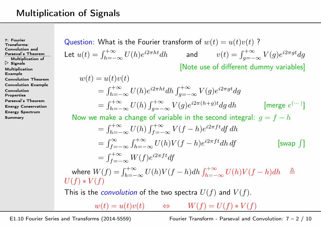
Multiplication of Signals
7: FourierTransforms:Convolution andParseval’s Theorem
⊲Multiplication ofSignals
MultiplicationExample
Convolution Theorem
Convolution Example
ConvolutionProperties
Parseval’s Theorem
Energy Conservation
Energy Spectrum
Summary
E1.10 Fourier Series and Transforms (2014-5559) Fourier Transform - Parseval and Convolution: 7 – 2 / 10
Question: What is the Fourier transform of w(t) = u(t)v(t) ?
Let u(t) =∫ +∞
h=−∞U(h)ei2πhtdh and v(t) =
∫ +∞
g=−∞V (g)ei2πgtdg
[Note use of different dummy variables]
w(t) = u(t)v(t)
=∫ +∞
h=−∞U(h)ei2πhtdh
∫ +∞
g=−∞V (g)ei2πgtdg
=∫ +∞
h=−∞U(h)
∫ +∞
g=−∞V (g)ei2π(h+g)tdg dh [merge e(··· )]
Now we make a change of variable in the second integral: g = f − h
=∫ +∞
h=−∞U(h)
∫ +∞
f=−∞V (f − h)ei2πftdf dh
=∫∞
f=−∞
∫ +∞
h=−∞U(h)V (f − h)ei2πftdh df [swap
∫
]
=∫ +∞
f=−∞W (f)ei2πftdf
where W (f) =∫ +∞
h=−∞U(h)V (f − h)dh
∫ +∞
h=−∞U(h)V (f − h)dh ,
U(f) ∗ V (f)
This is the convolution of the two spectra U(f) and V (f).
w(t) = u(t)v(t) ⇔ W (f) = U(f) ∗ V (f)

Multiplication Example
7: FourierTransforms:Convolution andParseval’s TheoremMultiplication ofSignals
⊲MultiplicationExample
Convolution Theorem
Convolution Example
ConvolutionProperties
Parseval’s Theorem
Energy Conservation
Energy Spectrum
Summary
E1.10 Fourier Series and Transforms (2014-5559) Fourier Transform - Parseval and Convolution: 7 – 3 / 10
u(t) =
e−at t ≥ 0
0 t < 0
U(f) = 1a+i2πf [from before]
v(t) = cos 2πFt
V (f) = 0.5 (δ(f + F ) + δ(f − F ))
w(t) = u(t)v(t)
W (f) = U(f) ∗ V (f)= 0.5
a+i2π(f+F ) +0.5
a+i2π(f−F )
If V (f) consists entirely of Dirac impulsesthen U(f) ∗ V (f) iust replaces each impulsewith a complete copy of U(f) scaled by thearea of the impulse and shifted so that 0Hzlies on the impulse. Then add theoverlapping complex spectra.
-5 0 50
0.5
1
Time (s)
u(t)
a=2
-5 0 50.10.20.30.40.5
Frequency (Hz)
|U(f
)|
-5 0 5-0.5
0
0.5
Frequence (Hz)
<U
(f)
(rad
/pi)
-5 0 5-1
0
1
Time (s)
v(t)
-5 0 50
0.20.4 F=2 0.5 0.5
Frequency (Hz)
|V(f
)|
-5 0 5-0.5
00.5
1
Time (s)
w(t
) a=2, F=2
-5 0 50
0.1
0.2
Frequency (Hz)
|W(f
)|
-5 0 5-0.5
0
0.5
Frequence (Hz)
<W
(f)
(rad
/pi)
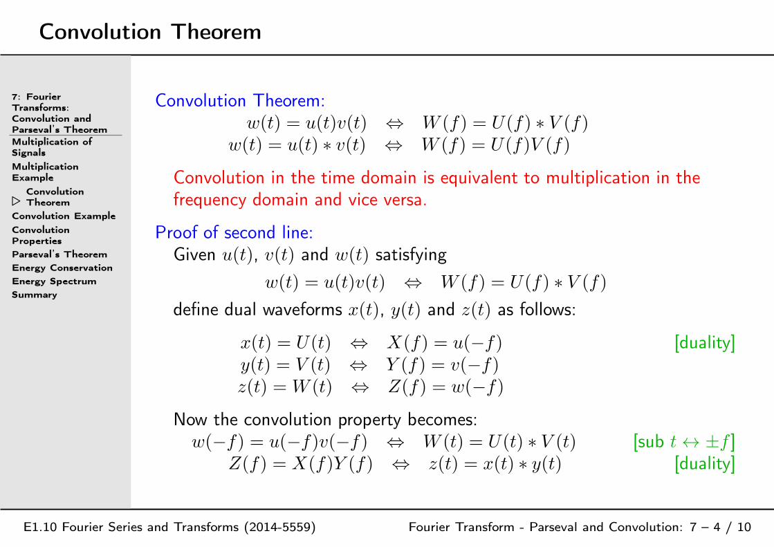
Convolution Theorem
7: FourierTransforms:Convolution andParseval’s TheoremMultiplication ofSignals
MultiplicationExample
⊲ConvolutionTheorem
Convolution Example
ConvolutionProperties
Parseval’s Theorem
Energy Conservation
Energy Spectrum
Summary
E1.10 Fourier Series and Transforms (2014-5559) Fourier Transform - Parseval and Convolution: 7 – 4 / 10
Convolution Theorem:w(t) = u(t)v(t) ⇔ W (f) = U(f) ∗ V (f)
w(t) = u(t) ∗ v(t) ⇔ W (f) = U(f)V (f)
Convolution in the time domain is equivalent to multiplication in thefrequency domain and vice versa.
Proof of second line:Given u(t), v(t) and w(t) satisfying
w(t) = u(t)v(t) ⇔ W (f) = U(f) ∗ V (f)
define dual waveforms x(t), y(t) and z(t) as follows:
x(t) = U(t) ⇔ X(f) = u(−f) [duality]y(t) = V (t) ⇔ Y (f) = v(−f)z(t) = W (t) ⇔ Z(f) = w(−f)
Now the convolution property becomes:w(−f) = u(−f)v(−f) ⇔ W (t) = U(t) ∗ V (t) [sub t ↔ ±f ]
Z(f) = X(f)Y (f) ⇔ z(t) = x(t) ∗ y(t) [duality]
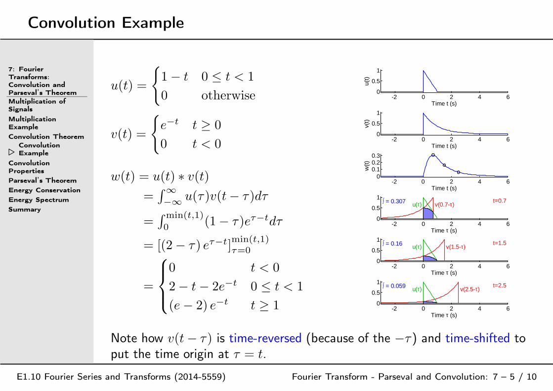
Convolution Example
7: FourierTransforms:Convolution andParseval’s TheoremMultiplication ofSignals
MultiplicationExample
Convolution Theorem
⊲ConvolutionExample
ConvolutionProperties
Parseval’s Theorem
Energy Conservation
Energy Spectrum
Summary
E1.10 Fourier Series and Transforms (2014-5559) Fourier Transform - Parseval and Convolution: 7 – 5 / 10
u(t) =
1− t 0 ≤ t < 1
0 otherwise
v(t) =
e−t t ≥ 0
0 t < 0
w(t) = u(t) ∗ v(t)
=∫∞
−∞u(τ )v(t− τ )dτ
=∫min(t,1)
0(1− τ )eτ−tdτ
= [(2− τ ) eτ−t]min(t,1)τ=0
=
0 t < 0
2− t− 2e−t 0 ≤ t < 1
(e− 2) e−t t ≥ 1
-2 0 2 4 60
0.5
1
Time t (s)
u(t)
-2 0 2 4 60
0.5
1
Time t (s)
v(t)
-2 0 2 4 60
0.10.20.3
Time t (s)
w(t
)
-2 0 2 4 60
0.5
1 t=0.7 v(0.7-τ)u(τ) ∫ = 0.307
Time τ (s)
-2 0 2 4 60
0.5
1 t=1.5 v(1.5-τ)u(τ) ∫ = 0.16
Time τ (s)
-2 0 2 4 60
0.5
1 t=2.5 v(2.5-τ)u(τ) ∫ = 0.059
Time τ (s)
Note how v(t− τ ) is time-reversed (because of the −τ ) and time-shifted toput the time origin at τ = t.
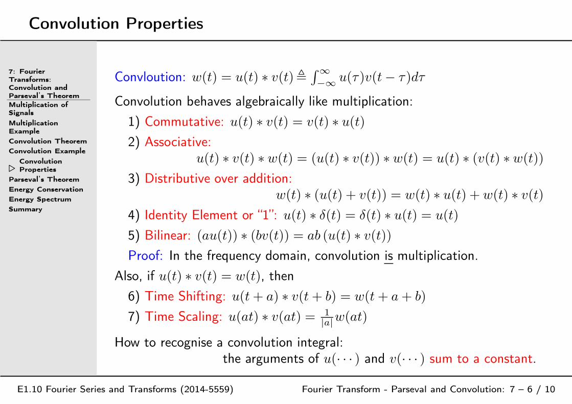
Convolution Properties
7: FourierTransforms:Convolution andParseval’s TheoremMultiplication ofSignals
MultiplicationExample
Convolution Theorem
Convolution Example
⊲ConvolutionProperties
Parseval’s Theorem
Energy Conservation
Energy Spectrum
Summary
E1.10 Fourier Series and Transforms (2014-5559) Fourier Transform - Parseval and Convolution: 7 – 6 / 10
Convloution: w(t) = u(t) ∗ v(t),∫∞
−∞u(τ )v(t− τ )dτ
Convolution behaves algebraically like multiplication:
1) Commutative: u(t) ∗ v(t) = v(t) ∗ u(t)
2) Associative:u(t) ∗ v(t) ∗ w(t) = (u(t) ∗ v(t)) ∗ w(t) = u(t) ∗ (v(t) ∗ w(t))
3) Distributive over addition:w(t) ∗ (u(t) + v(t)) = w(t) ∗ u(t) + w(t) ∗ v(t)
4) Identity Element or “1”: u(t) ∗ δ(t) = δ(t) ∗ u(t) = u(t)
5) Bilinear: (au(t)) ∗ (bv(t)) = ab (u(t) ∗ v(t))
Proof: In the frequency domain, convolution is multiplication.
Also, if u(t) ∗ v(t) = w(t), then
6) Time Shifting: u(t+ a) ∗ v(t+ b) = w(t+ a+ b)
7) Time Scaling: u(at) ∗ v(at) = 1|a|w(at)
How to recognise a convolution integral:the arguments of u(· · · ) and v(· · · ) sum to a constant.
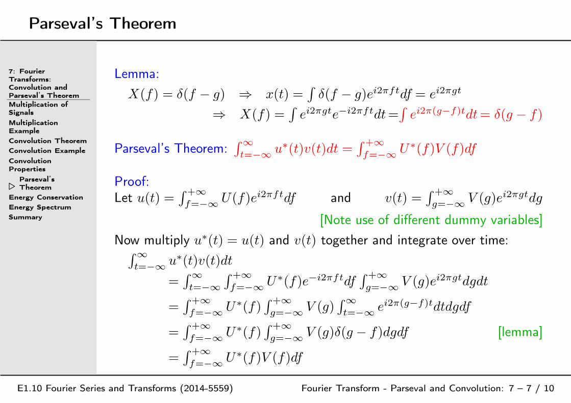
Parseval’s Theorem
7: FourierTransforms:Convolution andParseval’s TheoremMultiplication ofSignals
MultiplicationExample
Convolution Theorem
Convolution Example
ConvolutionProperties
⊲Parseval’sTheorem
Energy Conservation
Energy Spectrum
Summary
E1.10 Fourier Series and Transforms (2014-5559) Fourier Transform - Parseval and Convolution: 7 – 7 / 10
Lemma:
X(f) = δ(f − g) ⇒ x(t) =∫
δ(f − g)ei2πftdf = ei2πgt
⇒ X(f) =∫
ei2πgte−i2πftdt=∫
ei2π(g−f)tdt= δ(g − f)
Parseval’s Theorem:∫∞
t=−∞u∗(t)v(t)dt =
∫ +∞
f=−∞U∗(f)V (f)df
Proof:Let u(t) =
∫ +∞
f=−∞U(f)ei2πftdf and v(t) =
∫ +∞
g=−∞V (g)ei2πgtdg
[Note use of different dummy variables]
Now multiply u∗(t) = u(t) and v(t) together and integrate over time:∫∞
t=−∞u∗(t)v(t)dt
=∫∞
t=−∞
∫ +∞
f=−∞U∗(f)e−i2πftdf
∫ +∞
g=−∞V (g)ei2πgtdgdt
=∫ +∞
f=−∞U∗(f)
∫ +∞
g=−∞V (g)
∫∞
t=−∞ei2π(g−f)tdtdgdf
=∫ +∞
f=−∞U∗(f)
∫ +∞
g=−∞V (g)δ(g − f)dgdf [lemma]
=∫ +∞
f=−∞U∗(f)V (f)df

Energy Conservation
7: FourierTransforms:Convolution andParseval’s TheoremMultiplication ofSignals
MultiplicationExample
Convolution Theorem
Convolution Example
ConvolutionProperties
Parseval’s Theorem
⊲EnergyConservation
Energy Spectrum
Summary
E1.10 Fourier Series and Transforms (2014-5559) Fourier Transform - Parseval and Convolution: 7 – 8 / 10
Parseval’s Theorem:∫∞
t=−∞u∗(t)v(t)dt =
∫ +∞
f=−∞U∗(f)V (f)df
For the special case v(t) = u(t), Parseval’s theorem becomes:∫∞
t=−∞u∗(t)u(t)dt =
∫ +∞
f=−∞U∗(f)U(f)df
⇒ Eu =∫∞
t=−∞|u(t)|2 dt =
∫ +∞
f=−∞|U(f)|2 df
Energy Conservation: The energy in u(t) equals the energy in U(f).
Example:
u(t) =
e−at t ≥ 0
0 t < 0⇒ Eu =
∫
|u(t)|2dt =
[
−e−2at
2a
]∞
0= 1
2a
U(f) = 1a+i2πf [from before]
⇒∫
|U(f)|2 df =∫
dfa2+4π2f2
=
[
tan−1( 2πfa )
2πa
]∞
−∞
= π2πa = 1
2a
-5 0 50
0.5
1
Time (s)
u(t)
a=2
-5 0 50.10.20.30.40.5
Frequency (Hz)
|U(f
)|
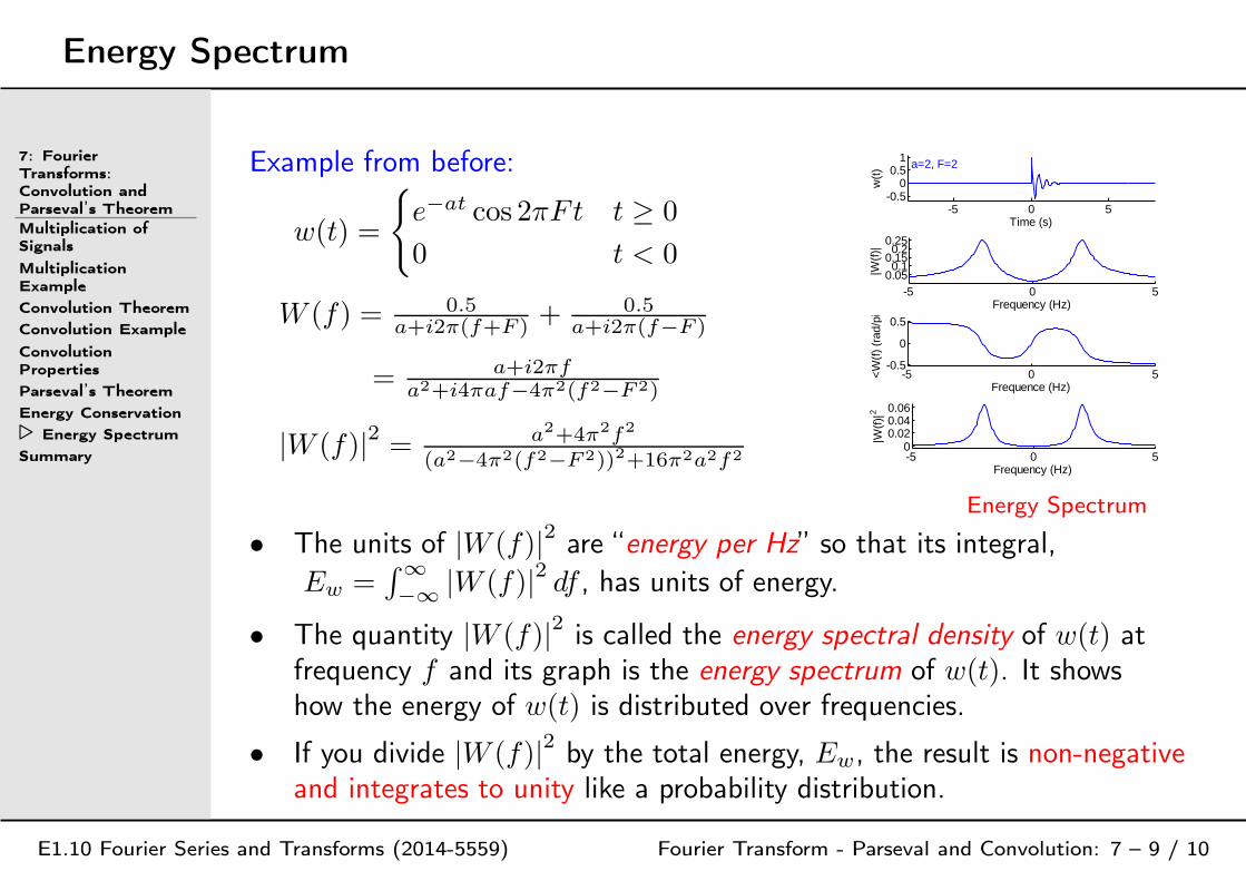
Energy Spectrum
7: FourierTransforms:Convolution andParseval’s TheoremMultiplication ofSignals
MultiplicationExample
Convolution Theorem
Convolution Example
ConvolutionProperties
Parseval’s Theorem
Energy Conservation
⊲ Energy Spectrum
Summary
E1.10 Fourier Series and Transforms (2014-5559) Fourier Transform - Parseval and Convolution: 7 – 9 / 10
Example from before:
w(t) =
e−at cos 2πFt t ≥ 0
0 t < 0
W (f) = 0.5a+i2π(f+F ) +
0.5a+i2π(f−F )
= a+i2πfa2+i4πaf−4π2(f2−F 2)
|W (f)|2 = a2+4π2f2
(a2−4π2(f2−F 2))2+16π2a2f2
-5 0 5-0.5
00.5
1
Time (s)
w(t
) a=2, F=2
-5 0 50.050.1
0.150.2
0.25
Frequency (Hz)
|W(f
)|
-5 0 5-0.5
0
0.5
Frequence (Hz)
<W
(f)
(rad
/pi)
-5 0 50
0.020.040.06
Frequency (Hz)
|W(f
)|2
Energy Spectrum
• The units of |W (f)|2
are “energy per Hz” so that its integral,
Ew =∫∞
−∞|W (f)|2 df , has units of energy.
• The quantity |W (f)|2
is called the energy spectral density of w(t) atfrequency f and its graph is the energy spectrum of w(t). It showshow the energy of w(t) is distributed over frequencies.
• If you divide |W (f)|2
by the total energy, Ew, the result is non-negativeand integrates to unity like a probability distribution.
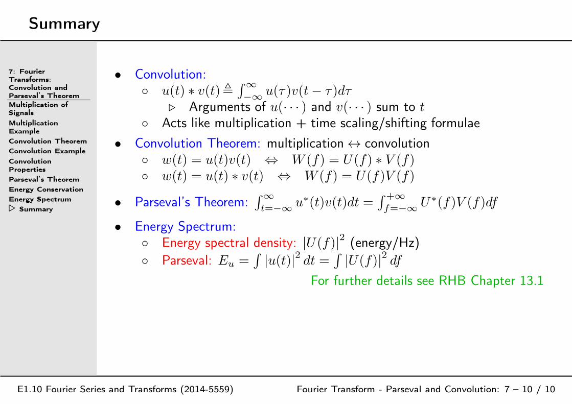
Summary
7: FourierTransforms:Convolution andParseval’s TheoremMultiplication ofSignals
MultiplicationExample
Convolution Theorem
Convolution Example
ConvolutionProperties
Parseval’s Theorem
Energy Conservation
Energy Spectrum
⊲ Summary
E1.10 Fourier Series and Transforms (2014-5559) Fourier Transform - Parseval and Convolution: 7 – 10 / 10
• Convolution: u(t) ∗ v(t),
∫∞
−∞u(τ )v(t− τ )dτ
⊲ Arguments of u(· · · ) and v(· · · ) sum to t
Acts like multiplication + time scaling/shifting formulae
• Convolution Theorem: multiplication ↔ convolution w(t) = u(t)v(t) ⇔ W (f) = U(f) ∗ V (f) w(t) = u(t) ∗ v(t) ⇔ W (f) = U(f)V (f)
• Parseval’s Theorem:∫∞
t=−∞u∗(t)v(t)dt =
∫ +∞
f=−∞U∗(f)V (f)df
• Energy Spectrum: Energy spectral density: |U(f)|2 (energy/Hz)
Parseval: Eu =∫
|u(t)|2dt =
∫
|U(f)|2df
For further details see RHB Chapter 13.1

8: Correlation
⊲ 8: Correlation
Cross-Correlation
Signal Matching
Cross-corr asConvolution
Normalized Cross-corr
AutocorrelationAutocorrelationexample
Fourier TransformVariants
Scale Factors
Summary
Spectrogram
E1.10 Fourier Series and Transforms (2015-5585) Fourier Transform - Correlation: 8 – 1 / 11

Cross-Correlation
8: Correlation
⊲ Cross-Correlation
Signal Matching
Cross-corr asConvolution
Normalized Cross-corr
AutocorrelationAutocorrelationexample
Fourier TransformVariants
Scale Factors
Summary
Spectrogram
E1.10 Fourier Series and Transforms (2015-5585) Fourier Transform - Correlation: 8 – 2 / 11
The cross-correlation between two signals u(t) and v(t) is
w(t) = u(t)⊗ v(t) ,∫∞−∞ u∗(τ )v(τ + t)dτ
=∫∞−∞ u∗(τ − t)v(τ )dτ [sub: τ → τ − t]
The complex conjugate, u∗(τ ) makes no difference if u(t) is real-valuedbut makes the definition work even if u(t) is complex-valued.
Correlation versus Convolution:
u(t)⊗ v(t) =∫∞−∞ u∗(τ )v(τ + t)dτ [correlation]
u(t) ∗ v(t) =∫∞−∞ u(τ )v(t− τ )dτ [convolution]
Unlike convolution, the integration variable, τ , has the same sign in thearguments of u(· · · ) and v(· · · ) so the arguments have a constantdifference instead of a constant sum (i.e. v(t) is not time-flipped).
Notes: (a) The argument of w(t) is called the “lag” (= delay of u versus v).(b) Some people write u(t) ⋆ v(t) instead of u(t)⊗ v(t).(c) Some swap u and v and/or negate t in the integral.
It is all rather inconsistent /.

Signal Matching
8: Correlation
Cross-Correlation
⊲ Signal Matching
Cross-corr asConvolution
Normalized Cross-corr
AutocorrelationAutocorrelationexample
Fourier TransformVariants
Scale Factors
Summary
Spectrogram
E1.10 Fourier Series and Transforms (2015-5585) Fourier Transform - Correlation: 8 – 3 / 11
Cross correlation is used to find where twosignals match: u(t) is the test waveform.
Example 1:v(t) contains u(t) with an unknown delay
and added noise.w(t) = u(t)⊗ v(t)
=∫u∗(τ − t)v(τ )dt gives a peak
at the time lag where u(τ − t) bestmatches v(τ ); in this case at t = 450
Example 2:y(t) is the same as v(t) with more noisez(t) = u(t)⊗ y(t) can still detect the
correct time delay (hard for humans)
Example 3:p(t) contains −u(t) so thatq(t) = u(t)⊗ p(t) has a negative peak
0 200 400 600
0
0.5
1
u(t)
0 200 400 600 800
0
0.5
1
v(t)
0 200 400 600 800
0
10
20
w(t
)
0 200 400 600 800
-202
y(t)
0 200 400 600 800-10
0
10
20
z(t)
0 200 400 600 800
-1
0
1
p(t)
0 200 400 600 800
-20
-10
0
q(t)
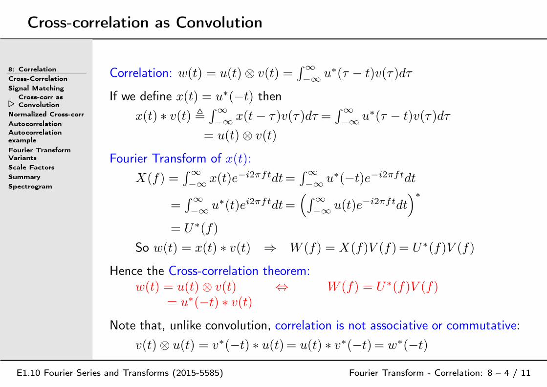
Cross-correlation as Convolution
8: Correlation
Cross-Correlation
Signal Matching
⊲Cross-corr asConvolution
Normalized Cross-corr
AutocorrelationAutocorrelationexample
Fourier TransformVariants
Scale Factors
Summary
Spectrogram
E1.10 Fourier Series and Transforms (2015-5585) Fourier Transform - Correlation: 8 – 4 / 11
Correlation: w(t) = u(t)⊗ v(t) =∫∞−∞ u∗(τ − t)v(τ )dτ
If we define x(t) = u∗(−t) then
x(t) ∗ v(t) ,∫∞−∞ x(t− τ )v(τ )dτ =
∫∞−∞ u∗(τ − t)v(τ )dτ
= u(t)⊗ v(t)
Fourier Transform of x(t):
X(f) =∫∞−∞ x(t)e−i2πftdt=
∫∞−∞ u∗(−t)e−i2πftdt
=∫∞−∞ u∗(t)ei2πftdt=
(∫∞−∞ u(t)e−i2πftdt
)∗
= U∗(f)
So w(t) = x(t) ∗ v(t) ⇒ W (f) = X(f)V (f)= U∗(f)V (f)
Hence the Cross-correlation theorem:w(t) = u(t)⊗ v(t) ⇔ W (f) = U∗(f)V (f)
= u∗(−t) ∗ v(t)Note that, unlike convolution, correlation is not associative or commutative:
v(t)⊗ u(t) = v∗(−t) ∗ u(t)= u(t) ∗ v∗(−t)= w∗(−t)
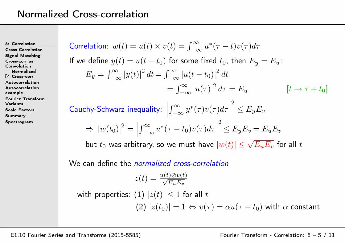
Normalized Cross-correlation
8: Correlation
Cross-Correlation
Signal Matching
Cross-corr asConvolution
⊲NormalizedCross-corr
AutocorrelationAutocorrelationexample
Fourier TransformVariants
Scale Factors
Summary
Spectrogram
E1.10 Fourier Series and Transforms (2015-5585) Fourier Transform - Correlation: 8 – 5 / 11
Correlation: w(t) = u(t)⊗ v(t) =∫∞−∞ u∗(τ − t)v(τ )dτ
If we define y(t) = u(t− t0) for some fixed t0, then Ey = Eu:
Ey =∫∞−∞ |y(t)|2 dt=
∫∞−∞ |u(t− t0)|2 dt=
∫∞−∞ |u(τ )|2 dτ = Eu [t → τ + t0]
Cauchy-Schwarz inequality:∣∣∣∫∞−∞ y∗(τ )v(τ )dτ
∣∣∣2
≤ EyEv
⇒ |w(t0)|2 =∣∣∣∫∞−∞ u∗(τ − t0)v(τ )dτ
∣∣∣2
≤ EyEv = EuEv
but t0 was arbitrary, so we must have |w(t)| ≤√EuEv for all t
We can define the normalized cross-correlation
z(t) = u(t)⊗v(t)√EuEv
with properties: (1) |z(t)| ≤ 1 for all t
(2) |z(t0)| = 1 ⇔ v(τ ) = αu(τ − t0) with α constant
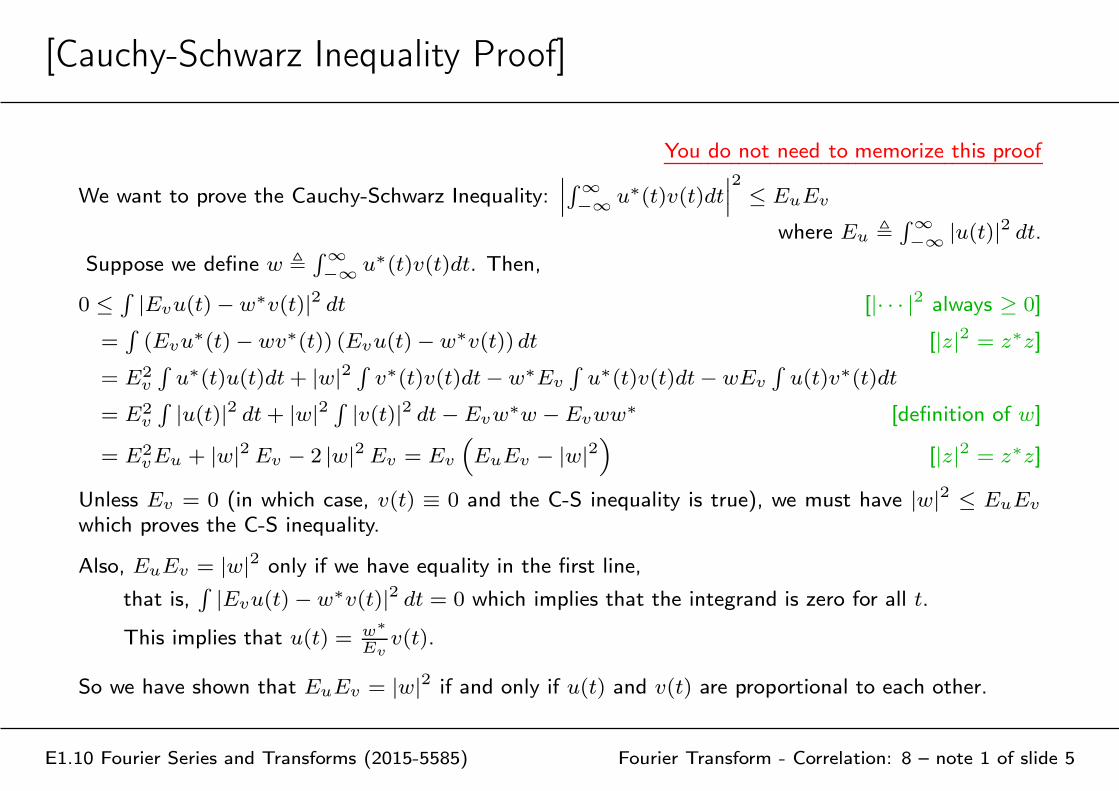
[Cauchy-Schwarz Inequality Proof]
E1.10 Fourier Series and Transforms (2015-5585) Fourier Transform - Correlation: 8 – note 1 of slide 5
You do not need to memorize this proof
We want to prove the Cauchy-Schwarz Inequality:∣
∣
∣
∫∞−∞ u∗(t)v(t)dt
∣
∣
∣
2≤ EuEv
where Eu ,∫∞−∞ |u(t)|2 dt.
Suppose we define w ,∫∞−∞ u∗(t)v(t)dt. Then,
0 ≤∫
|Evu(t)− w∗v(t)|2 dt [|· · · |2 always ≥ 0]
=∫
(Evu∗(t)− wv∗(t)) (Evu(t)− w∗v(t)) dt [|z|2 = z∗z]
= E2v
∫
u∗(t)u(t)dt+ |w|2∫
v∗(t)v(t)dt− w∗Ev
∫
u∗(t)v(t)dt− wEv
∫
u(t)v∗(t)dt
= E2v
∫
|u(t)|2 dt+ |w|2∫
|v(t)|2 dt− Evw∗w − Evww∗ [definition of w]
= E2vEu + |w|2 Ev − 2 |w|2 Ev = Ev
(
EuEv − |w|2)
[|z|2 = z∗z]
Unless Ev = 0 (in which case, v(t) ≡ 0 and the C-S inequality is true), we must have |w|2 ≤ EuEv
which proves the C-S inequality.
Also, EuEv = |w|2 only if we have equality in the first line,
that is,∫
|Evu(t)− w∗v(t)|2 dt = 0 which implies that the integrand is zero for all t.
This implies that u(t) = w∗
Evv(t).
So we have shown that EuEv = |w|2 if and only if u(t) and v(t) are proportional to each other.
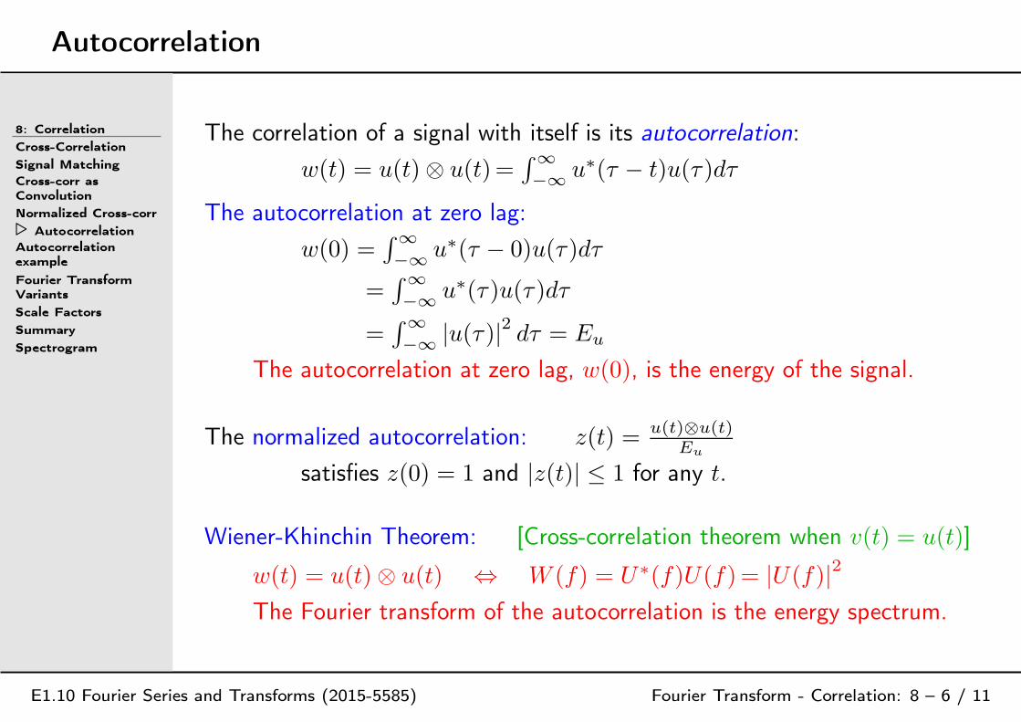
Autocorrelation
8: Correlation
Cross-Correlation
Signal Matching
Cross-corr asConvolution
Normalized Cross-corr
⊲ AutocorrelationAutocorrelationexample
Fourier TransformVariants
Scale Factors
Summary
Spectrogram
E1.10 Fourier Series and Transforms (2015-5585) Fourier Transform - Correlation: 8 – 6 / 11
The correlation of a signal with itself is its autocorrelation:
w(t) = u(t)⊗ u(t)=∫∞−∞ u∗(τ − t)u(τ )dτ
The autocorrelation at zero lag:
w(0) =∫∞−∞ u∗(τ − 0)u(τ )dτ
=∫∞−∞ u∗(τ )u(τ )dτ
=∫∞−∞ |u(τ )|2 dτ = Eu
The autocorrelation at zero lag, w(0), is the energy of the signal.
The normalized autocorrelation: z(t) = u(t)⊗u(t)Eu
satisfies z(0) = 1 and |z(t)| ≤ 1 for any t.
Wiener-Khinchin Theorem: [Cross-correlation theorem when v(t) = u(t)]
w(t) = u(t)⊗ u(t) ⇔ W (f) = U∗(f)U(f)= |U(f)|2
The Fourier transform of the autocorrelation is the energy spectrum.
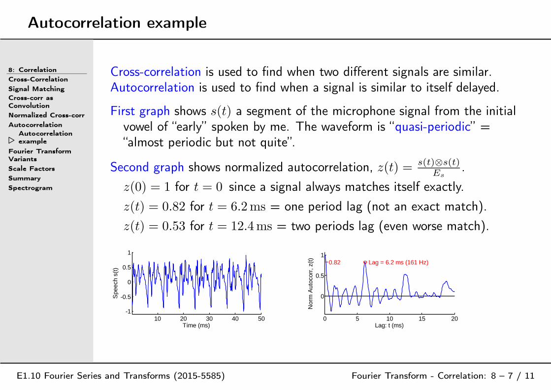
Autocorrelation example
8: Correlation
Cross-Correlation
Signal Matching
Cross-corr asConvolution
Normalized Cross-corr
Autocorrelation
⊲Autocorrelationexample
Fourier TransformVariants
Scale Factors
Summary
Spectrogram
E1.10 Fourier Series and Transforms (2015-5585) Fourier Transform - Correlation: 8 – 7 / 11
Cross-correlation is used to find when two different signals are similar.Autocorrelation is used to find when a signal is similar to itself delayed.
First graph shows s(t) a segment of the microphone signal from the initialvowel of “early” spoken by me. The waveform is “quasi-periodic” =“almost periodic but not quite”.
Second graph shows normalized autocorrelation, z(t) = s(t)⊗s(t)Es
.
z(0) = 1 for t = 0 since a signal always matches itself exactly.
z(t) = 0.82 for t = 6.2ms = one period lag (not an exact match).
z(t) = 0.53 for t = 12.4ms = two periods lag (even worse match).
10 20 30 40 50-1
-0.5
0
0.5
1
Spe
ech
s(t)
Time (ms)0 5 10 15 20
0
0.5
1Lag = 6.2 ms (161 Hz)0.82
Nor
m A
utoc
orr,
z(t
)
Lag: t (ms)

Fourier Transform Variants
8: Correlation
Cross-Correlation
Signal Matching
Cross-corr asConvolution
Normalized Cross-corr
AutocorrelationAutocorrelationexample
⊲Fourier TransformVariants
Scale Factors
Summary
Spectrogram
E1.10 Fourier Series and Transforms (2015-5585) Fourier Transform - Correlation: 8 – 8 / 11
There are three different versions of the Fourier Transform in current use.
(1) Frequency version (we have used this in lectures)
U(f) =∫∞−∞ u(t)e−i2πftdt u(t) =
∫∞−∞ U(f)ei2πftdf
• Used in the communications/broadcasting industry and textbooks.• The formulae do not need scale factors of 2π anywhere. ,,,
(2) Angular frequency version
U(ω) =∫∞−∞ u(t)e−iωtdt u(t) = 1
2π
∫∞−∞ U(ω)eiωtdω
Continuous spectra are unchanged: U(ω) = U(f) = U( ω2π )
However δ-function spectral components are multiplied by 2π so thatU(f) = δ(f − f0) ⇒ U(ω) = 2π × δ(ω − 2πf0)
• Used in most signal processing and control theory textbooks.
(3) Angular frequency + symmetrical scale factor
U(ω) = 1√2π
∫∞−∞ u(t)e−iωtdt u(t) = 1√
2π
∫∞−∞ U(ω)eiωtdω
In all cases U(ω) = 1√2π
U(ω)
• Used in many Maths textbooks (mathematicians like symmetry)

Scale Factors
8: Correlation
Cross-Correlation
Signal Matching
Cross-corr asConvolution
Normalized Cross-corr
AutocorrelationAutocorrelationexample
Fourier TransformVariants
⊲ Scale Factors
Summary
Spectrogram
E1.10 Fourier Series and Transforms (2015-5585) Fourier Transform - Correlation: 8 – 9 / 11
Fourier Transform using Angular Frequency:
U(ω) =∫∞−∞ u(t)e−iωtdt u(t) = 1
2π
∫∞−∞ U(ω)eiωtdω
Any formula involving∫df will change to 1
2π
∫dω [since dω = 2πdf ]
Parseval’s Theorem:∫u∗(t)v(t)dt = 1
2π
∫U∗(ω)V (ω)dω
Eu =∫|u(t)|2 dt = 1
2π
∫ ∣∣∣U(ω)∣∣∣2
dω
Waveform Multiplication: (convolution implicitly involves integration)
w(t) = u(t)v(t) ⇒ W (ω) = 12π U(ω) ∗ V (ω)
Spectrum Multiplication: (multiplication ; integration)
w(t) = u(t) ∗ v(t) ⇒ W (ω) = U(ω)V (ω)
To obtain formulae for version (3) of the Fourier Transform, U(ω),
substitute into the above formulae: U(ω) =√2πU(ω).

Summary
8: Correlation
Cross-Correlation
Signal Matching
Cross-corr asConvolution
Normalized Cross-corr
AutocorrelationAutocorrelationexample
Fourier TransformVariants
Scale Factors
⊲ Summary
Spectrogram
E1.10 Fourier Series and Transforms (2015-5585) Fourier Transform - Correlation: 8 – 10 / 11
• Cross-Correlation: w(t) = u(t)⊗ v(t)=∫∞−∞ u∗(τ − t)v(τ )dτ
Used to find similarities between v(t) and a delayed u(t)
Cross-correlation theorem: W (f) = U∗(f)V (f)
Cauchy-Schwarz Inequality: |u(t)⊗ v(t)| ≤√EuEv
⊲ Normalized cross-correlation:∣∣∣u(t)⊗v(t)√
EuEv
∣∣∣ ≤ 1
• Autocorrelation: x(t) = u(t)⊗ u(t)=∫∞−∞ u∗(τ − t)u(τ )dτ ≤ Eu
Wiener-Khinchin: X(f) = energy spectral density, |U(f)|2
Used to find periodicity in u(t)
• Fourier Transform using ω:
Continuous spectra unchanged; spectral impulses multiplied by 2π
In formulae:∫df → 1
2π
∫dω; ω-convolution involves an integral
For further details see RHB Chapter 13.1

Spectrogram
8: Correlation
Cross-Correlation
Signal Matching
Cross-corr asConvolution
Normalized Cross-corr
AutocorrelationAutocorrelationexample
Fourier TransformVariants
Scale Factors
Summary
⊲ Spectrogram
E1.10 Fourier Series and Transforms (2015-5585) Fourier Transform - Correlation: 8 – 11 / 11
Spectrogram of “Merry Christmas” spoken by Mike Brookes
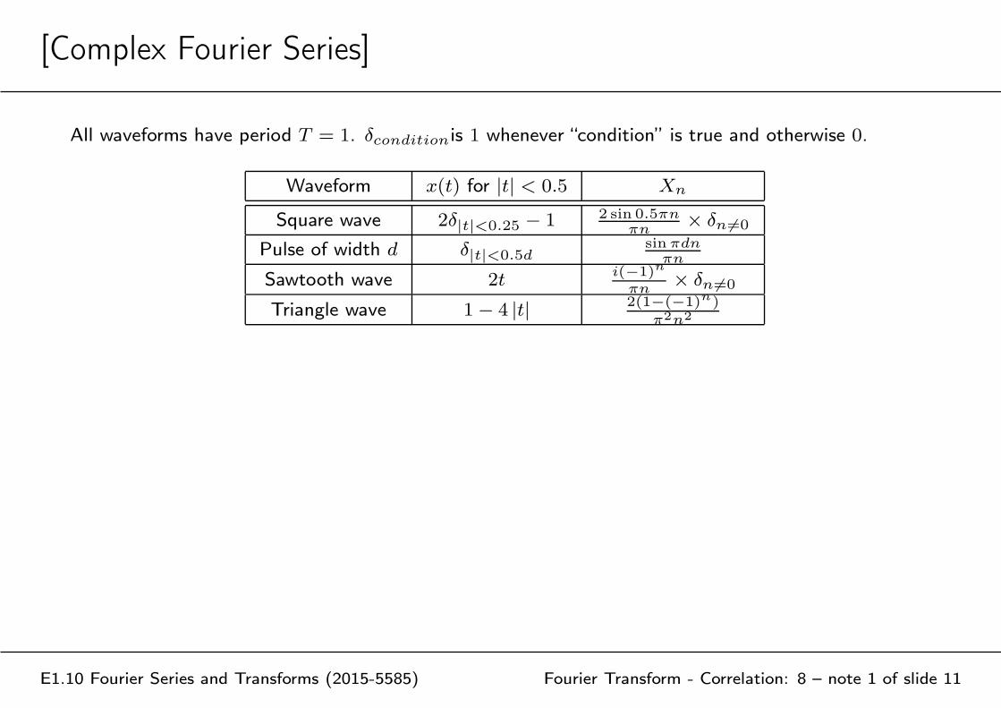
[Complex Fourier Series]
E1.10 Fourier Series and Transforms (2015-5585) Fourier Transform - Correlation: 8 – note 1 of slide 11
All waveforms have period T = 1. δconditionis 1 whenever “condition” is true and otherwise 0.
Waveform x(t) for |t| < 0.5 Xn
Square wave 2δ|t|<0.25 − 1 2 sin 0.5πnπn
× δn 6=0
Pulse of width d δ|t|<0.5dsinπdn
πn
Sawtooth wave 2ti(−1)n
πn× δn 6=0
Triangle wave 1− 4 |t|2(1−(−1)n)
π2n2
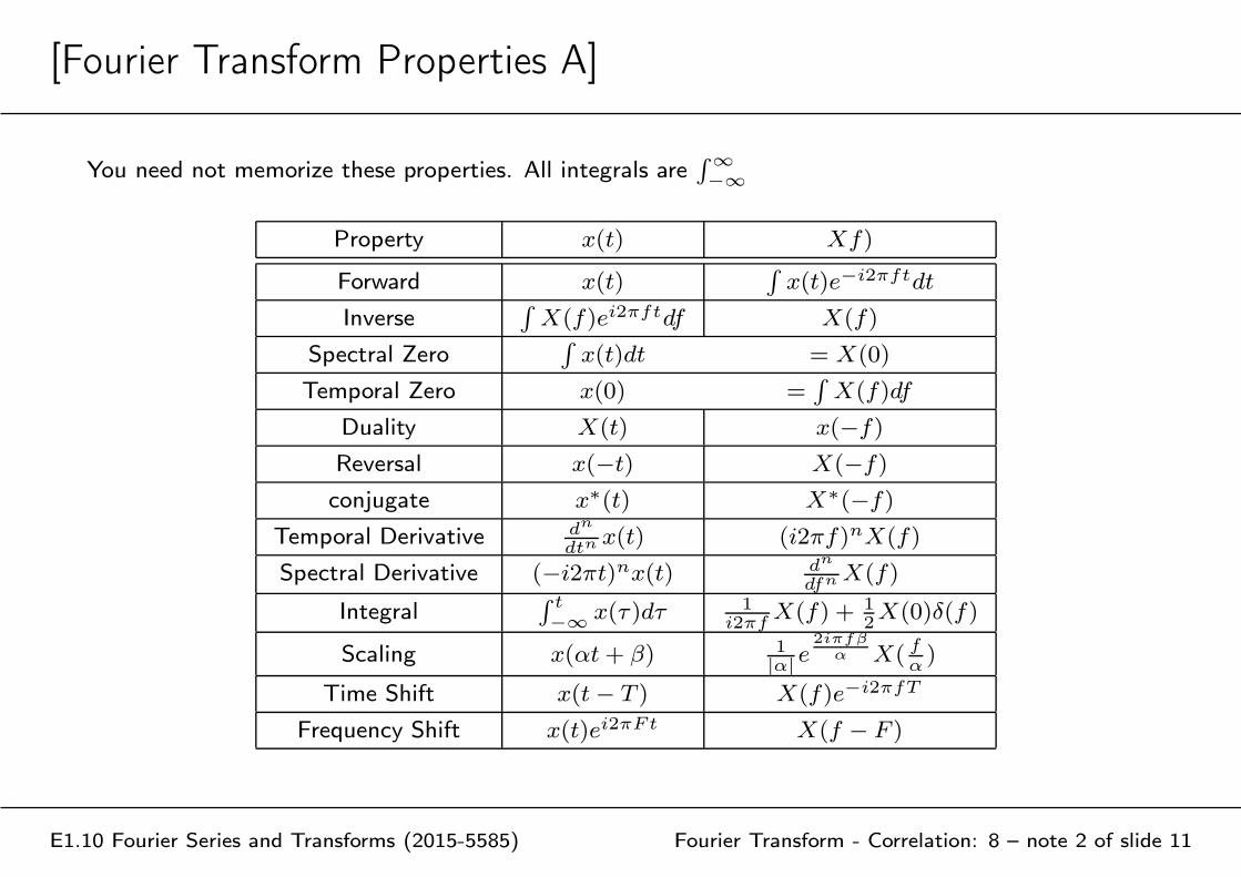
[Fourier Transform Properties A]
E1.10 Fourier Series and Transforms (2015-5585) Fourier Transform - Correlation: 8 – note 2 of slide 11
You need not memorize these properties. All integrals are∫∞−∞
Property x(t) Xf)
Forward x(t)∫
x(t)e−i2πftdt
Inverse∫
X(f)ei2πftdf X(f)
Spectral Zero∫
x(t)dt = X(0)
Temporal Zero x(0) =∫
X(f)df
Duality X(t) x(−f)
Reversal x(−t) X(−f)
conjugate x∗(t) X∗(−f)
Temporal Derivative dn
dtnx(t) (i2πf)nX(f)
Spectral Derivative (−i2πt)nx(t) dn
dfn X(f)
Integral∫ t
−∞ x(τ)dτ 1i2πf
X(f) + 12X(0)δ(f)
Scaling x(αt+ β) 1|α|
e2iπfβ
α X( f
α)
Time Shift x(t− T ) X(f)e−i2πfT
Frequency Shift x(t)ei2πFt X(f − F )
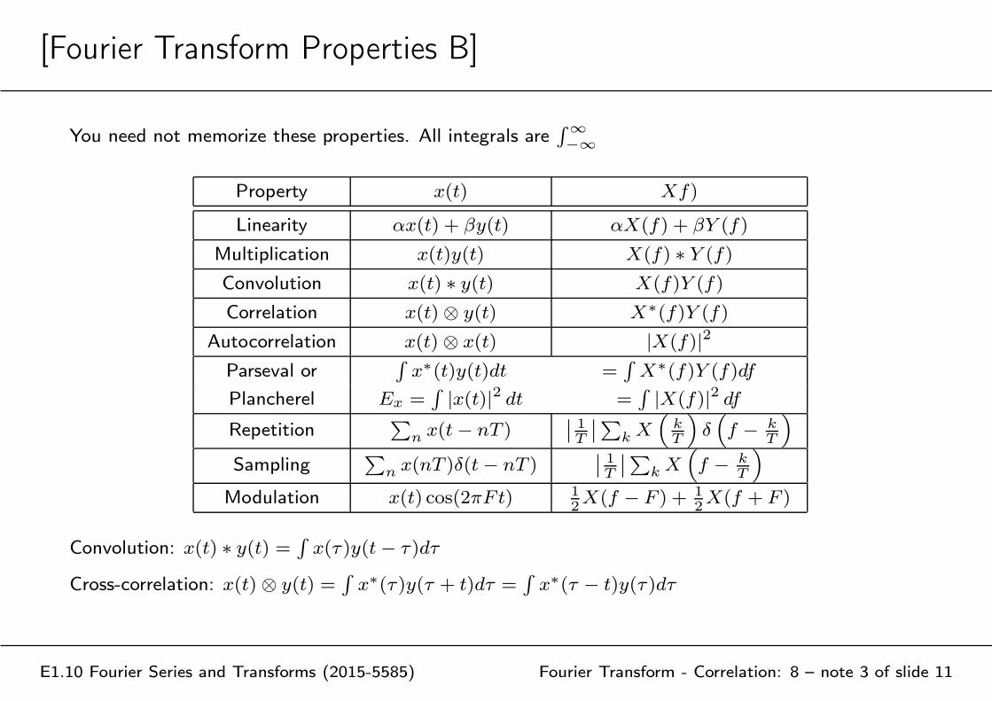
[Fourier Transform Properties B]
E1.10 Fourier Series and Transforms (2015-5585) Fourier Transform - Correlation: 8 – note 3 of slide 11
You need not memorize these properties. All integrals are∫∞−∞
Property x(t) Xf)
Linearity αx(t) + βy(t) αX(f) + βY (f)
Multiplication x(t)y(t) X(f) ∗ Y (f)
Convolution x(t) ∗ y(t) X(f)Y (f)
Correlation x(t)⊗ y(t) X∗(f)Y (f)
Autocorrelation x(t)⊗ x(t) |X(f)|2
Parseval or∫
x∗(t)y(t)dt =∫
X∗(f)Y (f)df
Plancherel Ex =∫
|x(t)|2 dt =∫
|X(f)|2 df
Repetition∑
n x(t− nT )∣
∣
1T
∣
∣
∑
k X(
kT
)
δ(
f − kT
)
Sampling∑
n x(nT )δ(t− nT )∣
∣
1T
∣
∣
∑
k X(
f − kT
)
Modulation x(t) cos(2πFt) 12X(f − F ) + 1
2X(f + F )
Convolution: x(t) ∗ y(t) =∫
x(τ)y(t− τ)dτ
Cross-correlation: x(t)⊗ y(t) =∫
x∗(τ)y(τ + t)dτ =∫
x∗(τ − t)y(τ)dτ
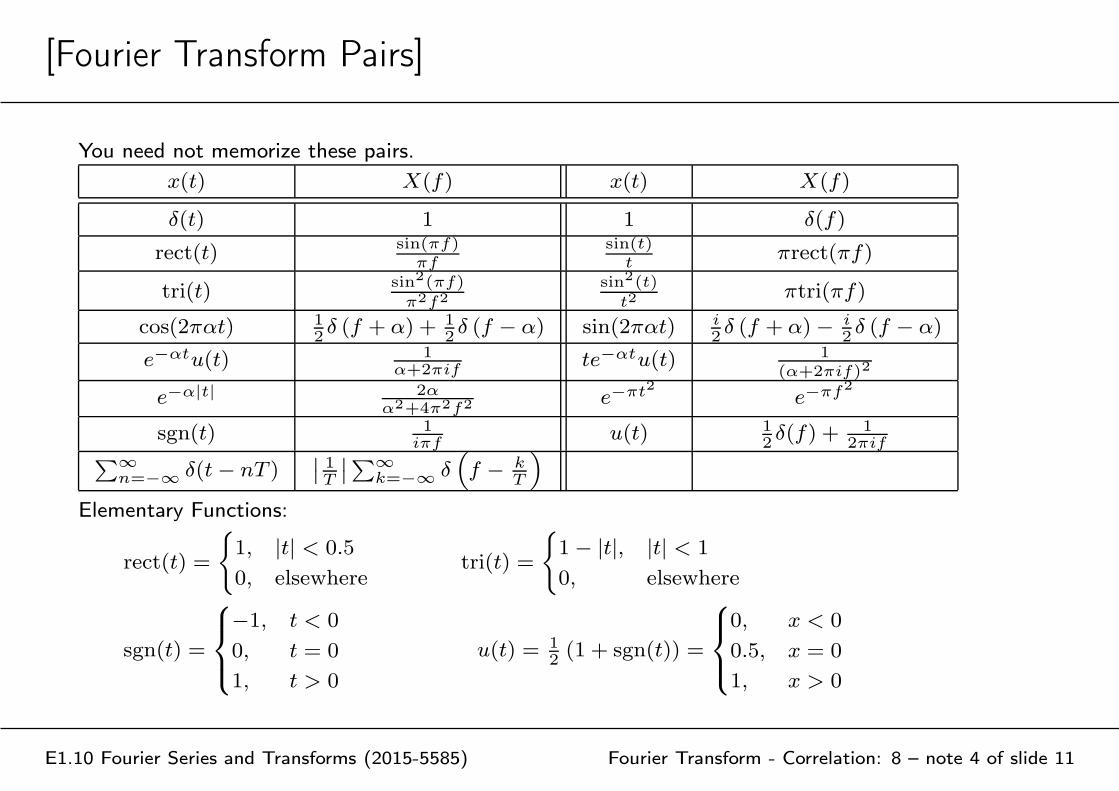
[Fourier Transform Pairs]
E1.10 Fourier Series and Transforms (2015-5585) Fourier Transform - Correlation: 8 – note 4 of slide 11
You need not memorize these pairs.
x(t) X(f) x(t) X(f)
δ(t) 1 1 δ(f)
rect(t)sin(πf)
πf
sin(t)t
πrect(πf)
tri(t)sin2(πf)
π2f2
sin2(t)
t2πtri(πf)
cos(2παt) 12δ (f + α) + 1
2δ (f − α) sin(2παt) i
2δ (f + α)− i
2δ (f − α)
e−αtu(t) 1α+2πif
te−αtu(t) 1(α+2πif)2
e−α|t| 2αα2+4π2f2
e−πt2 e−πf2
sgn(t) 1iπf
u(t) 12δ(f) + 1
2πif∑∞
n=−∞ δ(t− nT )∣
∣
1T
∣
∣
∑∞k=−∞ δ
(
f − kT
)
Elementary Functions:
rect(t) =
1, |t| < 0.5
0, elsewheretri(t) =
1− |t|, |t| < 1
0, elsewhere
sgn(t) =
−1, t < 0
0, t = 0
1, t > 0
u(t) = 12(1 + sgn(t)) =
0, x < 0
0.5, x = 0
1, x > 0