microsoft word - haiti ldsf report 20 june 12.docx word - haiti ldsf report 20 june 12.docx
TRANSCRIPT
LANDSCAPE BASELINE ASSESSMENT PORT-À-PIMENT WATERSHED January 2012

Prepared by the Earth Institute at Columbia University for the Ministry of Agriculture, Natural Resources and Rural Development (MARNDR) and the Community of Port-à-Piment watershed through the financial support of the United National Environment Program (UNEP) and the Earth Institute at Columbia University.
PORT-À-PIMENT LANDSCAPE BASELINE ASSESSMENT Prepared by: Sean Smukler, Joseph Muhlhuasen, Lucner Charlestra, Alex Fischer, Marc Levy, Cheryl Palm, Clare Sullivan, and Kate Tully, Jean Elie Thys, Jean Bonhomme Edouard, Saphinia Sannon, Jean Joseph Moncoeur, Yvon Alcegaire, Louis Jean Jacques Vanel, Ronald Saint Cyr Special Recognition and Thanks American University of the Caribbean United Nations Environment Program Groupe d’initiative pour un port a piment nouveau (GIPPN) Foundation Macaya Ministre d’Agriculture, des Resource Naturalles, et du Développement Rurale Special Thanks World Agroforestry Centre (ICRAF) Soil-Plant Spectral Diagnostics Laboratory facility in Nairobi, Kenya United States Natural Resource Conservation Service (NRCS) Soils Laboratory, Lincoln, Nebraska

3
Contents
Figures and Tables 4
EXECUTIVE SUMMARY 8
LIST OF ACRONYMS AND ABBREVIATIONS 13
INTRODUCTION 15 Soils and their role in agriculture development 17 A unique and effective methodology: the Land Degradation Surveillance Framework (LDSF) 19 Enabling Land Use Planning and Analysis in the Port-‐à-‐Piment Watershed 20
METHODS 22 Project Site 22 LDSF Methodology 24
RESULTS AND DISCUSSION 35
Landscape Characteristics, Use and Cover 35 Slope 35 Land Use /Land Cover 37 Vegetation 39 Visible Signs of Soil Erosion 42
Soil Properties 45 Chemical Properties 48 Physical properties 82
MAJOR FINDINGS, RECOMMENDATIONS AND NEXT STEPS 93 Key Problems 93 Recommendations 94 Conclusions and Next Steps 104
LITERATURE CITED 106
APPENDICES 109
Appendix I Soil Analysis Methods 109
Appendix II Land Use Land Cover Analysis Methods 110

4
Figures and Tables TABLE 1. VEGETATION, MANAGEMENT AND SOIL INDICATORS OBSERVED AND ANALYZED IN THE
LAND DEGRADATION SURVEILLANCE FRAMEWORK 25 TABLE 2. SOIL PHYSICAL AND CHEMICAL INDICATORS FROM THE LDSF AND THEIR IMPORTANCE
FOR AGRICULTURAL PRODUCTIONS (BRADY AND WEIL 2002, FAGERIA 2009; LINDSAY 1972). 28
TABLE 3. RECOMMENDED SLOPE LIMITS (%SLOPE) FOR AGRICULTURAL MANAGEMENT PRACTICES BASED ON INPUT INTENSITY (FAO 1993) 31
TABLE 4. LAND USE LAND COVER CLASSES DETERMINED BY FIELD DATA, DEFINITIONS AND AN EXAMPLE OF WHAT THEY LOOK LIKE IN THE FIELD. 33
TABLE 6. MEANS AND STANDARD ERROR OF THE MEANS OF SOIL PROPERTIES PREDICTED BY THE PARTIAL LEAST SQUARES (PLS) MODEL OF MID-‐ AND NEAR INFRARED (MIR AND NIR) SPECTROSCOPY FOR TOPSOIL (0-‐20 CM), N = 144, AND SUBSOIL (20-‐50 CM), N = 139. MODELS ARE ASSESSED BY THE COEFFICIENT OF DETERMINATION (R2) THE NUMBER OF PRINCIPLE COMPONENTS (PCS) AND ROOT MEAN SQUARE ERROR (RMSE). MODEL CONFIDENCE (LOW, MEDIUM AND HIGH) IS DETERMINED BY THE R2 VALUE. 47
TABLE 7. MODEL RESULTS FOR GEOSTATISTICAL ANALYSIS OF SELECT SOIL PROPERTIES THAT WERE USED TO DEVELOP DIGITAL SOIL MAPS. MODELS ARE ASSESSED BY THE ROOT MEAN SQUARE, AND THE AVERAGE STANDARD ERROR. 48
TABLE 9: GENERALIZED RECOMMENDATIONS FOR PRODUCTION PRIORITIES AND SOIL MANAGEMENT PRACTICES FOR THE REGIONS SURROUNDING MAJOR VILLAGES IN THE WATERSHED. SOIL MANAGEMENT RECOMMENDATIONS INCLUDE FERTILIZER (FERT.), INTEGRATED SOIL FERTILITY MANAGEMENT (ISFM), SOIL CONSERVATION (SC), OR AMENDMENTS (A). 103
FIGURE 1. WATERSHEDS HAVE THE POTENTIAL TO PROVIDE A NUMBER OF ECOSYSTEM SERVICES
THAT ARE ESSENTIAL FOR ENSURING HUMAN WELL-‐BEING (MA, 2005). 16 FIGURE 2. A LAND MANAGEMENT DECISION FRAMEWORK BASED ON THE ELEVATION, PROXIMITY
TO WATERWAY, SOIL EROSION RISK, AND SOIL CONSTRAINTS. 22 FIGURE 3. THE LOCATION OF THE PORT-‐À-‐PIMENT WATERSHED IN THE WESTERN COASTAL
REGION OF THE DEPARTMENT OF THE SOUTH. 23 FIGURE 4. MEAN MONTHLY RAINFALL (MM) AT CAMP-‐PERRIN FROM 1925 TO 2008, PORT-‐À-‐
PIMENT FROM 1925-‐1961, AND EXTRAPOLATED VALUES FOR PORT-‐À-‐PIMENT 1962-‐2008. 24 FIGURE 5. THE LDSF METHOD UTILIZES A HIERARCHICAL SAMPLING STRATEGY THAT ENABLES A
STATISTICALLY ROBUST EXTRAPOLATION FROM THE SUBPLOT AND PLOT TO THE LANDSCAPE. 26
FIGURE 6. WORKFLOW FOR THE IKONOS HIGH-‐RESOLUTION SATELLITE IMAGERY ANALYSIS DESIGNED TO PRODUCE A CONTINUOUS LAND USE/LAND COVER MAP OF THE ENTIRE WATERSHED. 32
FIGURE 7. MAP ILLUSTRATING THE DISTRIBUTION OF SLOPE (IN PERCENT) FOR THE WATERSHED DELINEATED (DASHED LINE) INTO UPPER (>500 M) AND LOWER WATERSHED (<500 M). 37
FIGURE 8. DISTRIBUTION OF LAND USES AND LAND COVER CLASSES AS ESTIMATED BY THE LDSF PLOT OBSERVATIONS AND REMOTE SENSING ANALYSIS. RESULTS ILLUSTRATE THE VAST MAJORITY OF THE LANDSCAPE IS USED FOR AGRICULTURAL PRODUCTION, EITHER AS AGROFORESTRY, CROPLAND OR PASTURE. 38
FIGURE 9. LAND USE LAND COVER MAP OF THE WATERSHED SHOWING WHAT LITTLE REMAINS OF FOREST COVER IS CONCENTRATED IN THE UPPER WATERSHED AT THE HIGHEST ELEVATIONS. 38
FIGURE 11. BOX PLOTS ILLUSTRATING THE LOWER QUARTILE (Q1), MEDIAN (Q2), UPPER QUARTILE (Q3), AND EXTREME VALUES (DOTS) FOR (A.) TREE DENSITY (B.) TREE BIOVOLUME AND (C.) PERCENT WOODY COVER BY LAND USE LAND COVER CLASSES ACROSS THE WATERSHED. 40
FIGURE 13. OBSERVED INCIDENCE OF SOIL EROSION ACROSS THE WATERSHED INDICATING EXTENSIVE SOIL LOSSES. 43
5
FIGURE 14. PERCENT DISTRIBUTION FOR THE INCIDENCE OF FIELD OBSERVED SOIL EROSION FOR EACH LULC CLASS. 44
FIGURE 15. OBSERVED INCIDENCE OF SOIL EROSION BY SLOPE CLASS. THE MOST SEVERE EROSION, GULLY, IS MOST PREVALENT ON STEEP SLOPES BUT IS FOUND THROUGHOUT THE WATERSHED. 45
FIGURE 16. BOX PLOTS ILLUSTRATING THE LOWER QUARTILE (Q1), MEDIAN (Q2), UPPER QUARTILE (Q3), AND EXTREME VALUES (DOTS) FOR SOIL ORGANIC CARBON (SOC) G KG-‐1 FOR TOPSOIL (0-‐20 CM) AND SUBSOIL (20-‐50 CM) BY LAND USE LAND COVER CLASS. 49
FIGURE 17. MAP OF THE DISTRIBUTION OF TOPSOIL (0-‐20 CM) SOIL ORGANIC CARBON (SOC) G KG-‐1. THE HIGHEST CONCENTRATION OF SOC WAS FOUND IN THE FORESTS AT THE TOP OF THE WATERSHED AND THE LOWEST IN THE SOUTHEAST. 51
FIGURE 18. BOX PLOTS ILLUSTRATING THE LOWER QUARTILE (Q1), MEDIAN (Q2), UPPER QUARTILE (Q3), AND EXTREME VALUES (DOTS) FOR SOIL TOTAL NITROGEN (N) G KG-‐1 FOR TOPSOIL (0-‐20 CM) AND SUBSOIL (20-‐50 CM) BY LAND USE LAND COVER CLASS. 53
FIGURE 19. MAP OF THE DISTRIBUTION OF TOPSOIL (0-‐20 CM) TOTAL NITROGEN (N) G KG-‐1. 53 FIGURE 20. BOX PLOTS ILLUSTRATING THE LOWER QUARTILE (Q1), MEDIAN (Q2), UPPER
QUARTILE (Q3), AND EXTREME VALUES (DOTS) FOR PH ON LEVEL, MODERATE OR STEEP SLOPES FOR (A) THE LOWER WATERSHED (<500 M) OR (B) UPPER WATERSHED (>500M) SITES. RED DASHED LINES ARE VALUES THAT INDICATE POTENTIAL CONSTRAINTS TO CROP PRODUCTIVITY. CROP GROWTH MAY BE LIMITED IN SOILS < 5.5 OR > 8.3 UNITS. 55
FIGURE 21. MAP OF THE DISTRIBUTION OF PREDICTIONS FOR TOPSOIL PH (0-‐20 CM) ILLUSTRATING ONLY A FEW AREAS OF EXTREMELY ACIDIC OR ALKALINE SOILS. 56
FIGURE 22. BOX PLOTS ILLUSTRATING THE LOWER QUARTILE (Q1), MEDIAN (Q2), UPPER QUARTILE (Q3), AND EXTREME VALUES (DOTS) FOR CATION EXCHANGE CAPACITY (CEC) CMOLC KG-‐1 ON LEVEL, MODERATE OR STEEP SLOPES FOR (A) LOW ELEVATION (<500 M) OR (B) HIGH ELEVATION (>500M) SITES. ALL OF THE VALUES ARE CONSIDERED HIGH AND NOT A CONSTRAINT FOR PRODUCTION. 57
FIGURE 23. MAP OF THE DISTRIBUTION OF PREDICTED TOPSOIL (0-‐20 CM) VALUES FOR CATION EXCHANGE CAPACITY (CEC) CMOLC KG-‐1. 58
FIGURE 24. BOX PLOTS ILLUSTRATING THE LOWER QUARTILE (Q1), MEDIAN (Q2), UPPER QUARTILE (Q3), AND EXTREME VALUES (DOTS) FOR EXCHANGEABLE CALCIUM (EXCH. CA) CMOLC KG-‐1 ON LEVEL, MODERATE OR STEEP SLOPES FOR (A) LOW ELEVATION (<500 M) OR (B) HIGH ELEVATION (>500M) SITES. NO VALUES WERE <2 CMOLC KG-‐1 (THE RED DASHED LINE) WHICH INDICATES THE CRITICAL VALUE BELOW WHICH EXCHA. CA MAY LIMIT CROP PRODUCTIVITY. 59
FIGURE 25. MAP OF THE DISTRIBUTION OF PREDICTED TOPSOIL (0-‐20 CM) VALUES FOR EXCHANGEABLE CALCIUM (EXCH. CA) CMOLC KG-‐1 60
FIGURE 26. BOX PLOTS ILLUSTRATING THE LOWER QUARTILE (Q1), MEDIAN (Q2), UPPER QUARTILE (Q3), AND EXTREME VALUES (DOTS) FOR EXCHANGEABLE MAGNESIUM (EXCH. MG) CMOLC KG-‐1 ON LEVEL, MODERATE OR STEEP SLOPES FOR (A) LOW ELEVATION (<500 M) OR (B) HIGH ELEVATION (>500M) SITES. 45% OF THE SOILS SAMPLED WERE < 5 CMOLC KG-‐1 (THE RED DASHED LINE) INDICATING EXCHA. MG MAY LIMIT CROP PRODUCTIVITY. 61
FIGURE 27. MAP OF THE DISTRIBUTION OF PREDICTED TOPSOIL (0-‐20 CM) VALUES FOR MAGNESIUM (EXCH. MG) CMOLC KG-‐1 62
FIGURE 28. BOX PLOTS ILLUSTRATING THE LOWER QUARTILE (Q1), MEDIAN (Q2), UPPER QUARTILE (Q3), AND EXTREME VALUES (DOTS) FOR EXCHANGEABLE POTASSIUM (EXCH. K) CONCENTRATIONS FOR TOPSOIL (0-‐20 CM) AND SUBSOIL (20-‐50 CM) BY LAND USE LAND COVER CLASS. NEARLY ALL OF THE AGRICULTURAL SOILS SAMPLED WERE < 0.5 CMOLC KG-‐1 (THE RED DASHED LINE) INDICATING EXCH. K MAY LIMIT CROP PRODUCTIVITY. 63
FIGURE 29. BOX PLOTS ILLUSTRATING THE LOWER QUARTILE (Q1), MEDIAN (Q2), UPPER QUARTILE (Q3), AND EXTREME VALUES (DOTS) FOR EXCHANGEABLE POTASSIUM (EXCH. K) CMOLC KG-‐1 ON LEVEL, MODERATE OR STEEP SLOPES FOR (A) LOW ELEVATION (<500 M) OR (B) HIGH ELEVATION (>500M) SITES. THE RED DASHED LINE INDICATES THE CRITICAL VALUE BELOW WHICH EXCHA. K < 0.5CMOLC KG-‐1 MAY LIMIT CROP PRODUCTIVITY. 64
6
FIGURE 30. MAP OF THE DISTRIBUTION OF (TOP) PREDICTED TOPSOIL (0-‐20 CM) VALUES FOR EXCHANGEABLE POTASSIUM (EXCH. K) CMOLC KG-‐1 AND (BOTTOM) AREAS BELOW THE CRITICAL THRESHOLD THAT MAY INDICATE POTENTIAL CONSTRAINTS FRO CROP PRODUCTION. 65
31. BOX PLOTS ILLUSTRATING THE LOWER QUARTILE (Q1), MEDIAN (Q2), UPPER QUARTILE (Q3), AND EXTREME VALUES (DOTS) FOR EXCHANGEABLE NA CMOLC KG-‐1 ON LEVEL, MODERATE OR STEEP SLOPES FOR (A) LOW ELEVATION (<500 M) OR (B) HIGH ELEVATION (>500M) SITES. THE RED DASHED LINE INDICATES THE CRITICAL VALUE ABOVE WHICH EXCHA. NA MAY NEGATIVELY IMPACT SOIL STRUCTURE (> 1 CMOLC KG-‐1). 66
FIGURE 32. MAP OF THE DISTRIBUTION OF PREDICTED TOPSOIL (0-‐20 CM) VALUES FOR EXCHANGEABLE NA CMOLC KG-‐1. 67
FIGURE 33. BOX PLOTS ILLUSTRATING THE LOWER QUARTILE (Q1), MEDIAN (Q2), UPPER QUARTILE (Q3), AND POSSIBLE OUTLIERS FOR MEHLICH-‐3 EXTRACTABLE PHOSPHORUS (M-‐3E P) MG KG-‐1 ON LEVEL, MODERATE OR STEEP SLOPES FOR (A) LOW ELEVATION (<500 M) OR (B) HIGH ELEVATION (>500M) SITES. SOILS WITH < 30 MG KG-‐1 OF M-‐3E P MAY LIMITED CROP PRODUCTIVITY (BOTTOM RED DASHED LINE). SOIL WITH > 50 MG KG-‐1 M-‐3E P MAY BE A RISK OF P LOSSES TO NEARBY WATERWAYS. 69
FIGURE 34. MAP OF THE DISTRIBUTION OF PREDICTED TOPSOIL (0-‐20 CM) VALUES FOR MEHLICH-‐3 EXTRACTABLE PHOSPHORUS (M-‐3E P) MG KG-‐1. 69
FIGURE 35. BOX PLOTS ILLUSTRATING THE LOWER QUARTILE (Q1), MEDIAN (Q2), UPPER QUARTILE (Q3), AND EXTREME VALUES (DOTS) FOR THE PHOSPHORUS SORPTION INDEX (PSI) ON LEVEL, MODERATE OR STEEP SLOPES FOR (A) LOW ELEVATION (<500 M) OR (B) HIGH ELEVATION (>500M) SITES. VALUES < 50 (BELOW THE LOWER RED DASHED LINE) INDICATE POTENTIAL RISK OF LOSING SOLUBLE PHOSPHORUS TO THE ENVIRONMENT THROUGH LEACHING. VALUES ABOVE THE UPPER RED DASHED LINE (>250) INDICATE POTENTIAL PHOSPHORUS FIXATION. 70
FIGURE 36. MAP OF THE DISTRIBUTION OF (TOP) PREDICTED TOPSOIL (0-‐20 CM) VALUES FOR THE PSI AND (BOTTOM) AREAS OF THE WATERSHED BELOW THE SUGGESTED CRITICAL THRESHOLD. 71
FIGURE 37. BOX PLOTS ILLUSTRATING THE LOWER QUARTILE (Q1), MEDIAN (Q2), UPPER QUARTILE (Q3), AND POSSIBLE OUTLIERS FOR MEHLICH-‐3 EXTRACTABLE SULFATE-‐SULFUR (M-‐3E S) MG KG-‐1 ON LEVEL, MODERATE OR STEEP SLOPES FOR (A) LOW ELEVATION (<500 M) OR (B) HIGH ELEVATION (>500M) SITES. RED DASHED LINES ARE VALUES THAT INDICATE POTENTIAL CONSTRAINTS TO CROP PRODUCTIVITY. CROP GROWTH MAY BE LIMITED IN SOILS < 10 MG KG-‐1. 73
FIGURE 38. MAP OF THE DISTRIBUTION OF (TOP) PREDICTED TOPSOIL (0-‐20 CM) VALUES FOR MEHLICH-‐3 EXTRACTABLE SULFATE-‐SULFUR (M-‐3E S) MG KG-‐1 AND (BOTTOM) THE DISTRIBUTION OF AREAS BELOW THE 10 MG KG-‐1 THRESHOLD THAT INDICATES POTENTIAL S DEFICIENCIES. 74
FIGURE 39. BOX PLOTS ILLUSTRATING THE LOWER QUARTILE (Q1), MEDIAN (Q2), UPPER QUARTILE (Q3), AND POSSIBLE OUTLIERS FOR MEHLICH-‐3 EXTRACTABLE COPPER (CU) MG KG-‐1 ON LEVEL, MODERATE OR STEEP SLOPES FOR (A) LOW ELEVATION (<500 M) OR (B) HIGH ELEVATION (>500M) SITES. RED DASHED LINES ARE VALUES THAT INDICATE POTENTIAL CONSTRAINTS TO CROP PRODUCTIVITY. CROP GROWTH MAY BE LIMITED IN SOILS < 1 MG KG-‐1 OR > 20 MG KG-‐1. 75
FIGURE 40. MAP OF THE DISTRIBUTION OF PREDICTED TOPSOIL (0-‐20 CM) VALUES MEHLICH-‐3 EXTRACTABLE COPPER (CU) MG KG-‐1. 76
FIGURE 41. BOX PLOTS ILLUSTRATING THE LOWER QUARTILE (Q1), MEDIAN (Q2), UPPER QUARTILE (Q3), AND POSSIBLE OUTLIERS FOR MEHLICH-‐3 EXTRACTABLE IRON (M-‐3E FE) MG KG-‐1 ON LEVEL, MODERATE OR STEEP SLOPES FOR (A) LOW ELEVATION (<500 M) OR (B) HIGH ELEVATION (>500M) SITES. RED DASHED LINES ARE VALUES THAT INDICATE POTENTIAL CONSTRAINTS TO CROP PRODUCTIVITY. CROP GROWTH MAY BE LIMITED IN SOILS < 50 MG KG-‐1 OR > 200 MG KG-‐1. 77
FIGURE 42. MAP OF THE DISTRIBUTION OF PREDICTED TOPSOIL (0-‐20 CM) VALUES FOR MEHLICH-‐3 EXTRACTABLE IRON (M-‐3E FE) MG KG-‐1. 78
7
FIGURE 43. BOX PLOTS ILLUSTRATING THE LOWER QUARTILE (Q1), MEDIAN (Q2), UPPER QUARTILE (Q3), AND POSSIBLE OUTLIERS FOR MEHLICH-‐3 EXTRACTABLE ZINC (M-‐3E ZN) MG KG-‐1 ON LEVEL, MODERATE OR STEEP SLOPES FOR (A) LOW ELEVATION (<500 M) OR (B) HIGH ELEVATION (>500M) SITES. RED DASHED LINES ARE VALUES THAT INDICATE POTENTIAL CONSTRAINTS TO CROP PRODUCTIVITY. CROP GROWTH MAY BE LIMITED IN SOILS < 4 MG KG-‐1 OR > 120 MG KG-‐1. 79
FIGURE 44. MAP OF THE DISTRIBUTION OF (TOP) PREDICTED TOPSOIL (0-‐20 CM) VALUES FOR MEHLICH-‐3 EXTRACTABLE ZINC (M-‐3E ZN) MG KG-‐1 AND (BOTTOM) THE DISTRIBUTION OF AREAS BELOW THE 4 MG KG-‐1 THRESHOLD THAT INDICATES THE POTENTIAL FOR ZN DEFICIENCY. 80
FIGURE 45. BOX PLOTS ILLUSTRATING THE LOWER QUARTILE (Q1), MEDIAN (Q2), UPPER QUARTILE (Q3), AND EXTREME VALUES (DOTS) FOR ELECTRICAL CONDUCTIVITY ON LEVEL, MODERATE OR STEEP SLOPES FOR (A) LOW ELEVATION (<500 M) OR (B) HIGH ELEVATION (>500M) SITES. ALL VALUES ARE FAR BELOW THE 2000 ΜS CM-‐1 THAT INDICATES POTENTIAL CONSTRAINTS TO CROP PRODUCTIVITY. 81
FIGURE 46. MAP OF THE DISTRIBUTION OF PREDICTED TOPSOIL (0-‐20 CM) VALUES FOR ELECTRICAL CONDUCTIVITY (EC) ΜS CM-‐1 INDICATING HIGHER VALUES AT THE TOP OF THE WATERSHED. 82
FIGURE 47. SOIL TEXTURE FOR TOPSOIL (0-‐20 CM) AND SUBSOIL (20-‐50 CM) IN TERMS OF (A) SAND, (B.) SILT AND (C.) CLAY FRACTION G KG-‐1 ON LEVEL, MODERATE OR STEEP SLOPES FOR (LEFT SIDE) LOW ELEVATION (<500 M) OR (RIGHT SIDE) HIGH ELEVATION (>500M) SITES. 83
FIGURE 48. MAP OF THE DISTRIBUTION OF PREDICTED SAND G KG-‐1CONTENT FOR TOPSOIL (0-‐20 CM). 84
FIGURE 49. MAP OF THE DISTRIBUTION OF PREDICTED SILT G KG-‐1CONTENT FOR TOPSOIL (0-‐20 CM). 84
FIGURE 50. MAP OF THE DISTRIBUTION OF PREDICTED CLAY G KG-‐1CONTENT FOR TOPSOIL (0-‐20 CM). 85
FIGURE 51. RELATIONSHIP BETWEEN INFILTRATION RATE AND TREE DENSITY ILLUSTRATING INCREASED INFILTRATION WITH HIGHER TREE DENSITY. 86
FIGURE 52. DEPTH TO RESTRICTION FOR PLANT ROOTS BY LAND USE LAND COVER CLASS (A.), ON LEVEL, MODERATE OR STEEP SLOPES FOR (B) LOW ELEVATION (<500 M) OR (C) HIGH ELEVATION (>500M) SITES. 88
53. MAP OF THE DISTRIBUTION OF DEPTH TO RESTRICTION FOR PLANT ROOTS INDICATING SHALLOW SOIL DEPTHS ON THE STEEPEST SLOPES IN THE UPPER WATERSHED. 89
FIGURE 54. MAP OF PREDICTED SOIL EROSION RATES ACROSS THE WATERSHED IN MG HA-‐1 YEAR-‐1. 90
FIGURE 55. MAP OF THE DISTRIBUTION OF THE SOIL CONSTRAINT INDEX BASED ON THE TOTAL NUMBER OF PREDICTED IMPEDIMENTS TO PLANT GROWTH. 92
FIGURE 56. POTENTIAL LAND MANAGEMENT DECISION TREE. FOUR DECISION NODES AND ASSOCIATED PRODUCTION PRIORITIES AND SOIL MANAGEMENT OPTIONS ARE ILLUSTRATED. PRODUCTION PRIORITIES INCLUDE CROPPING SYSTEMS 1-‐4*, PERENNIALS (1-‐4*), PASTURE OR NATURAL REGENERATION. SOIL MANAGEMENT OPTIONS INCLUDE FERTILIZER (FERT.), INTEGRATED SOIL FERTILITY MANAGEMENT (ISFM), SOIL CONSERVATION (SC), OR AMENDMENTS (A). *PRIORITIES ARE CLASSIFIED INTO DISTINCT SYSTEMS (I.E. 1-‐4). 96

8
Executive summary The Port-‐à-‐Piment Landscape Baseline Assessment provides a comprehensive bio-‐physical inventory of the roughly 100 km2 watershed of the town of Port-‐à-‐Piment, in Southwest Haiti. This study provides an analysis of the key factors that indicate the productivity and health of the ecosystem including the spatial distribution of soil, land use/land cover and vegetation conditions across the watershed. These indicators provide a basis for determining the availability of key ecosystem services. Ecosystem services are the ecological functions that contribute to human well-‐being, such as the purification of water, the stabilization and regeneration of soil and production of food, fuel and fiber. The Landscape Baseline Assessment presented here is a first step towards supporting a science-‐based approach to ecosystem service management as an integral component to regional sustainable development efforts. This data and analysis provide great opportunities for further analysis and community engagement in watershed management planning. The specific objectives of this study are to:
1. Develop a set of tools to immediately inform participatory planning for improved watershed management including: maps of key watershed and ecosystem health indicators; site-‐specific information on crop and tree production requirement and limitations; and a decision framework for land management recommendations.
2. Provide data to assess the availability of ecosystem services to enhance long-‐term planning
3. Establish baseline measurements to monitor and assess land management impacts and ecosystem health over time.
4. Propose a set of targets and/or threshold levels for key indicators to ensure the continued availability of ecosystem services.
The Landscape Baseline Assessment was a collaborative effort among a number of local universities, governmental, and non-‐governmental organizations, the United Nations Environment Programme, soil labs in the United States and Kenya and the Earth Institute at Columbia University. A team spent five weeks in the field observing vegetation conditions, land use, and visible erosion and taking soil samples. Soil samples were analyzed for a suite of physical and chemical properties. Analyses of these data were designed to provide an understanding of the landscape status based on easily discernible characteristics, either by land use, elevation or topography. The aim is to provide some generalizable and straightforward management recommendations. The analysis also provides spatially explicit analysis of these findings as digital maps that can be used to provide very site-‐specific information on the health of soil and vegetation throughout the watershed. Key problems identified in the analysis included:
9
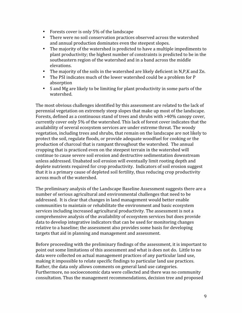
• Forests cover is only 5% of the landscape • There were no soil conservation practices observed across the watershed
and annual production dominates even the steepest slopes. • The majority of the watershed is predicted to have a multiple impediments to
plant productivity; the highest number of constraints is predicted to be in the southeastern region of the watershed and in a band across the middle elevations.
• The majority of the soils in the watershed are likely deficient in N,P,K and Zn. • The PSI indicates much of the lower watershed could be a problem for P
absorption • S and Mg are likely to be limiting for plant productivity in some parts of the
watershed. The most obvious challenges identified by this assessment are related to the lack of perennial vegetation on extremely steep slopes that make up most of the landscape. Forests, defined as a continuous stand of trees and shrubs with >40% canopy cover, currently cover only 5% of the watershed. This lack of forest cover indicates that the availability of several ecosystem services are under extreme threat. The woody vegetation, including trees and shrubs, that remain on the landscape are not likely to protect the soil, regulate floods, or provide adequate woodfuel for cooking or the production of charcoal that is rampant throughout the watershed. The annual cropping that is practiced even on the steepest terrain in the watershed will continue to cause severe soil erosion and destructive sedimentation downstream unless addressed. Unabated soil erosion will eventually limit rooting depth and deplete nutrients required for crop productivity. Indicators of soil erosion suggest that it is a primary cause of depleted soil fertility, thus reducing crop productivity across much of the watershed. The preliminary analysis of the Landscape Baseline Assessment suggests there are a number of serious agricultural and environmental challenges that need to be addressed. It is clear that changes in land management would better enable communities to maintain or rehabilitate the environment and basic ecosystem services including increased agricultural productivity. The assessment is not a comprehensive analysis of the availability of ecosystem services but does provide data to develop integrative indicators that can be used for monitoring changes relative to a baseline; the assessment also provides some basis for developing targets that aid in planning and management and assessment. Before proceeding with the preliminary findings of the assessment, it is important to point out some limitations of this assessment and what is does not do. Little to no data were collected on actual management practices of any particular land use, making it impossible to relate specific findings to particular land use practices. Rather, the data only allows comments on general land use categories. Furthermore, no socioeconomic data were collected and there was no community consultation. Thus the management recommendations, decision tree and proposed
10
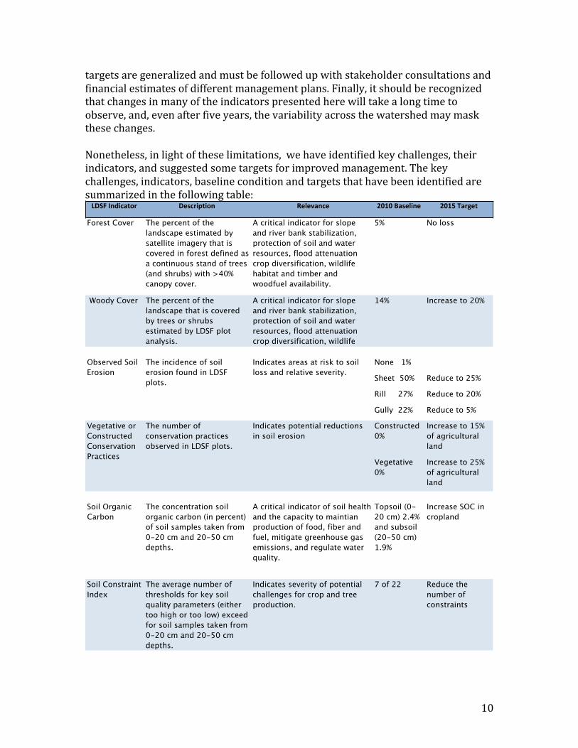
targets are generalized and must be followed up with stakeholder consultations and financial estimates of different management plans. Finally, it should be recognized that changes in many of the indicators presented here will take a long time to observe, and, even after five years, the variability across the watershed may mask these changes. Nonetheless, in light of these limitations, we have identified key challenges, their indicators, and suggested some targets for improved management. The key challenges, indicators, baseline condition and targets that have been identified are summarized in the following table:
!"#$%&'()*+,-. "/0*.)1,)-' %%2/3/4+'*/ 5676%8+0/3)'/ 5679%:+.;/,%
Forest Cover The percent of the landscape estimated by satellite imagery that is covered in forest defined as a continuous stand of trees (and shrubs) with >40% canopy cover.
A critical indicator for slope and river bank stabilization, protection of soil and water resources, flood attenuation crop diversification, wildlife habitat and timber and woodfuel availability.
5% No loss
Woody Cover The percent of the landscape that is covered by trees or shrubs estimated by LDSF plot analysis.
A critical indicator for slope and river bank stabilization, protection of soil and water resources, flood attenuation crop diversification, wildlife habitat and timber and
14% Increase to 20%
None 1%
Sheet 50% Reduce to 25%
Rill 27% Reduce to 20%
Gully 22% Reduce to 5%
Constructed 0%
Increase to 15% of agricultural land
Vegetative 0%
Increase to 25% of agricultural land
Soil Organic Carbon
The concentration soil organic carbon (in percent) of soil samples taken from 0-20 cm and 20-50 cm depths.
A critical indicator of soil health and the capacity to maintian production of food, fiber and fuel, mitigate greenhouse gas emissions, and regulate water quality.
Topsoil (0-20 cm) 2.4% and subsoil (20-50 cm) 1.9%
Increase SOC in cropland
Soil Constraint Index
The average number of thresholds for key soil quality parameters (either too high or too low) exceed for soil samples taken from 0-20 cm and 20-50 cm depths.
Indicates severity of potential challenges for crop and tree production.
7 of 22 Reduce the number of constraints
The incidence of soil erosion found in LDSF plots.
Indicates areas at risk to soil loss and relative severity.
The number of conservation practices observed in LDSF plots.
Indicates potential reductions in soil erosion
Vegetative or Constructed Conservation Practices
Observed Soil Erosion

11
A key outcome of this report would be to use the baseline analysis and proposed targets to engage with stakeholders to develop management plans and targets that are readily observable and directly linked to those presented here. For example, this would include setting a target for the number of trees to be planted in the watershed based on the land area in need of woody cover identified by this analysis. The target should also reflect the financial constraints of the project and the reality of how much community involvement can be expected. The management plans would then require monitoring activities for targets, such as seedlings survival and even tree growth, which will not necessarily be observed in a follow-‐up Landscape Assessments (i.e. many of the trees may be too small to be counted based on the protocol use here). This analysis is only the first step of many to provide an effective set of tools for stakeholders in Port-‐à-‐Piment to better understand and manage their environment for ecosystem services and improved livelihoods. Further analysis of this data will provide a more detailed assessment of the validity of the soil predictions and include confidence bounds for these predictions. While the analysis at the watershed provides an important overall picture of the conditions present, analysis or soil characteristics and soil erosion risk at a smaller scale (e.g. the sub-‐watershed or village area) may be critical for prioritizing actions by community groups. Targeted land management strategies to address and reverse the environmental degradation, including reforestation, rehabilitation of depleted soils for improved crop production for food security and income generation will accompany this analysis; a first draft of recommendations are included in this report. These data and the land use and soil management recommendations that accompany them can also be further refined and reanalyzed in an iterative process with stakeholder consultation. Initial consultations prior to the publication of this report highlighted the following recommendations (not in any order of priority):
• Promote agroforestry practices as they are key to address the deforestation problem in the area and can also mitigate soil degradation if managed properly. Priority trees that have commercial values are coffee, citrus, pigeon pea and avocado.
• Establish woodlots on farm lands for charcoal production • Establish nurseries in key locations in the watershed to facilitate distribution
to farmers. The mountainous areas of Nan Gauvin and Cavalier were identified as priority locations.
• Launch a vast campaign of soil conservation at the watershed scale with different incentive strategies (e.g. participatory, cash/food for work)

12
• Promote improved pasture management and animal husbandry as a means to diversify income and reduce pressure on natural resource.
13
LIST OF ACRONYMS AND ABBREVIATIONS Al Aluminum AEZ Agroecological Zone B Boron C Carbon Ca Calcium Cmolc Centimole of charge CEC Cation exchange capacity
CNIGS République D'Haïti Ministere de la Planification et de La Cooperation Externe
CSI Cote Sud Initiative CU Columbia University Cu Copper DBH Diameter at breast height EC Electrical conductivity EI The Earth Institute (at Columbia University) Fe Iron FAO Food and Agriculture Organization GIS Geographic information system Ha Hectare ICRAF World Agroforestry Center K Potassium LDSF Land Degradation Surveillance Framework LULC Land use land cover MA Millennium Ecosystem Assessment MDG Millennium Development Goals MVP Millennium Villages Project Mg Magnesium MIR Mid-‐infrared Mn Manganese M-‐3e Mehlich-‐3 exchangeable N Nitrogen NGO(s) Non-‐governmental organization(s) NIR Near-‐infrared P Phosphorus pH Soil acidity RDR Root depth restrictions S Sulfur SAR Sodium absorption ratio SOC Soil organic carbon

14
TropAg Tropical Agriculture and Rural Environment Program (of the EI) µS cm-‐1 Microsiemens per centimeter Zn Zinc
15
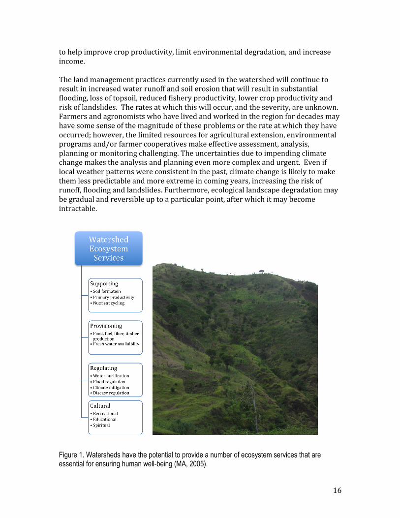
Introduction The Port-‐à-‐Piment watershed, located in the Department of the South, the southwestern-‐most department of Haiti, is characterized by steep mountainous terrain. Once forested, this area is now largely dominated by the annual crop production of poor smallholder farmers. The watershed borders the Pic Macaya National Park,1 one of the few remaining stands of contiguous forest in the country. Within the watershed, despite the steep terrain, farmers mainly grow annual crops, such as maize, beans and cassava for subsistence, and there is little evidence of investment in higher value cash crops or soil stabilizing perennial crops. The combination of annual cropping and deforestation has resulted in substantial, and, in some cases, severe soil erosion on the steep slopes that dominate the landscape. The harvest of annual crops every season leaves soil bare for extensive periods of time, which are thus susceptible to wind and water erosion. Current grazing practices also contribute to the lack of vegetation cover on high-‐risk soils. Furthermore, charcoal production is extensive in the middle and upper areas of the watershed and threatens what remains of the forest cover. Despite the obvious risk of soil loss, only a small number of farmers are utilizing soil conservation measures. If current land management practices continue, there will be a continued reduction in crop yields, decreased wood availability and an end to charcoal production and the loss of other benefits produced from an ecologically functional watershed. When these ecological functions are impaired by poor management practices, ecosystem services are diminished (Figure 1). Of particular concern in Port-‐à-‐Piment are the potential losses of ecosystem services related to food and fuel provisioning and hydrologic processes such as flood regulation and water purification. Despite the considerable reliance on these ecosystem services to ensure the livelihoods of those living in Port-‐à-‐Piment, there is little understanding of how the availability of these services might be changing. There are no recent or real-‐time monitoring systems in Haiti for environmental resources, ecosystems, or soil characteristics. The last land use land cover analysis done at a national scale was completed using 1999 imagery by the Centre National d’Information Geo Spatiale (CNIGS). Currently there are no monitoring systems for assessing changes in landscape scale ecosystem services or environment conditions. The lack of soil surveillance and testing remains a major limiting factor for agricultural extension agents and their efforts to provide farmers with information
1 Pic Macaya National Park is counted as one of the principal protected areas in Haiti due to its high biodiversity, large forest system, and its important role as a water catchment in the larger ecosystem of the Southern Peninsula. Its role as a water catchment played a role in its designation as a protected area in 1983, originally counted as 2000 acres. Its boundaries, however, remain ambiguously defined and a source of community contention (Toussaint 2008).
16
to help improve crop productivity, limit environmental degradation, and increase income. The land management practices currently used in the watershed will continue to result in increased water runoff and soil erosion that will result in substantial flooding, loss of topsoil, reduced fishery productivity, lower crop productivity and risk of landslides. The rates at which this will occur, and the severity, are unknown. Farmers and agronomists who have lived and worked in the region for decades may have some sense of the magnitude of these problems or the rate at which they have occurred; however, the limited resources for agricultural extension, environmental programs and/or farmer cooperatives make effective assessment, analysis, planning or monitoring challenging. The uncertainties due to impending climate change makes the analysis and planning even more complex and urgent. Even if local weather patterns were consistent in the past, climate change is likely to make them less predictable and more extreme in coming years, increasing the risk of runoff, flooding and landslides. Furthermore, ecological landscape degradation may be gradual and reversible up to a particular point, after which it may become intractable.
Figure 1. Watersheds have the potential to provide a number of ecosystem services that are essential for ensuring human well-being (MA, 2005).

17
To provide land use managers -‐-‐ whether smallholder farmers, agricultural extension agents, or development professionals -‐-‐ with more recent information on the environment to enable better targeted planning and management, we undertook an intensive biophysical inventory of the watershed utilizing the Land Degradation Surveillance Framework (LDSF) (Vågen et al. 2010). The specific objectives of this study were to provide a baseline assessment of soil and vegetation characteristics and condition (or health) at a landscape scale in order to:
1. Develop a set of tools to immediately inform participatory planning for improved watershed management including: maps of key watershed and ecosystem health indicators; site specific information on crop and tree production requirement and limitations; and a decision framework for land management recommendations.
2. Provide data to assess the availability of ecosystem services to enhance long-‐term planning
3. Establish baseline measurements to monitor and assess land management impacts and ecosystem health over time.
4. Propose a set of targets and/or threshold levels for key indicators to ensure the continued availability of ecosystem services.
In this report, we present preliminary results that begin to address the first objective. In combination with other research activities such as crop and tree trials, and hydrologic and climatic observations, greater resolution will be provided for the first objective and enable the second. This study provides the baseline data for the third objective, which can immediately inform the development of targets for key indicators and planning. Follow up assessments will be required to monitor changes and track targets. Here we provide a brief background for how and why this study was undertaken, details on the specific methods of data collection and analysis, results and a preliminary set of recommendations and targets. The analysis of this data focused on developing management recommendations for readily discernible landscape characteristics such as land use/ cover, the slope or the elevation of the watershed. The data presented here should be used to help establish, through community consultation, development targets that meet the objectives of local stakeholders, and enhance continued participatory planning and monitoring efforts.
Soils and their role in agriculture development Soil is a key component of the terrestrial ecosystem. A number of ecological functions are dependent on the condition of soil. Many of these functions are considered ecosystem services when directly beneficial to humans . Thus functioning soils are critical for ensuring the availability of a number of ecosystem services including (Smukler et al. 2012):
18
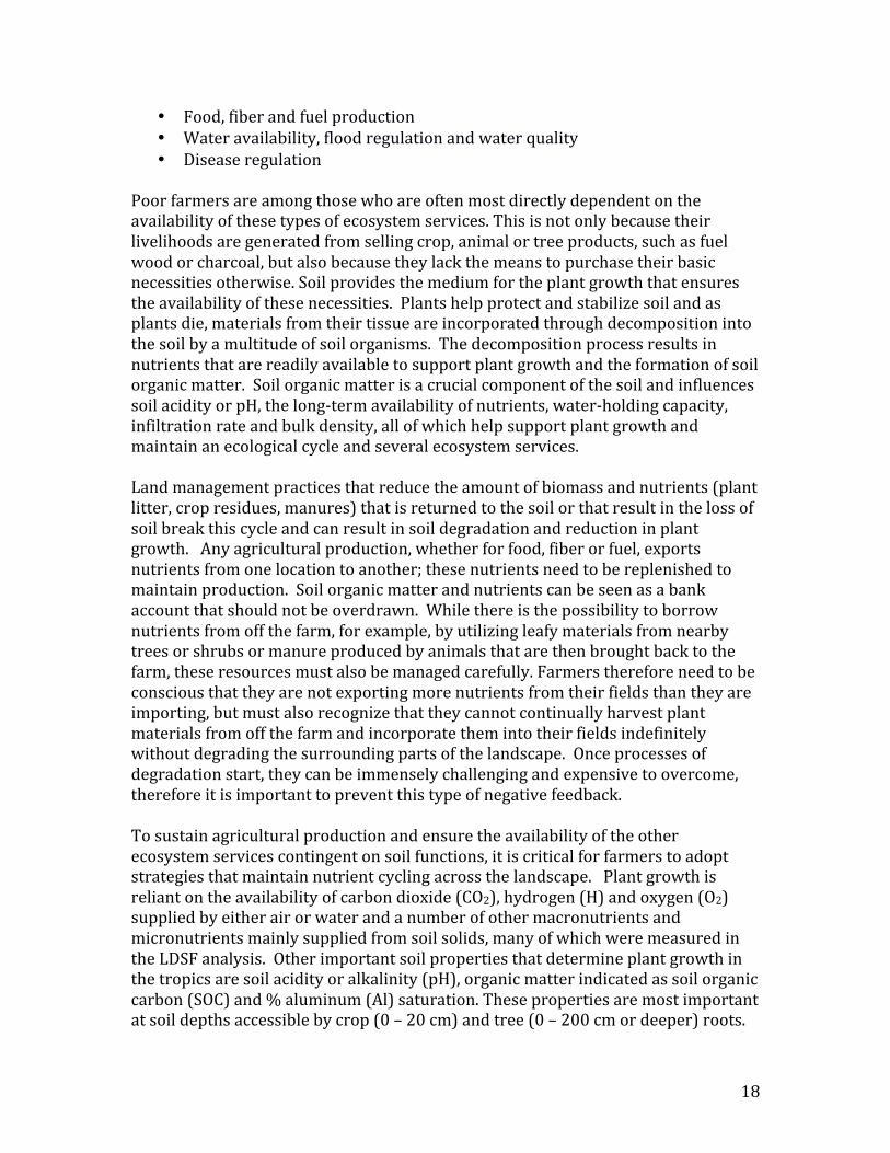
• Food, fiber and fuel production • Water availability, flood regulation and water quality • Disease regulation
Poor farmers are among those who are often most directly dependent on the availability of these types of ecosystem services. This is not only because their livelihoods are generated from selling crop, animal or tree products, such as fuel wood or charcoal, but also because they lack the means to purchase their basic necessities otherwise. Soil provides the medium for the plant growth that ensures the availability of these necessities. Plants help protect and stabilize soil and as plants die, materials from their tissue are incorporated through decomposition into the soil by a multitude of soil organisms. The decomposition process results in nutrients that are readily available to support plant growth and the formation of soil organic matter. Soil organic matter is a crucial component of the soil and influences soil acidity or pH, the long-‐term availability of nutrients, water-‐holding capacity, infiltration rate and bulk density, all of which help support plant growth and maintain an ecological cycle and several ecosystem services. Land management practices that reduce the amount of biomass and nutrients (plant litter, crop residues, manures) that is returned to the soil or that result in the loss of soil break this cycle and can result in soil degradation and reduction in plant growth. Any agricultural production, whether for food, fiber or fuel, exports nutrients from one location to another; these nutrients need to be replenished to maintain production. Soil organic matter and nutrients can be seen as a bank account that should not be overdrawn. While there is the possibility to borrow nutrients from off the farm, for example, by utilizing leafy materials from nearby trees or shrubs or manure produced by animals that are then brought back to the farm, these resources must also be managed carefully. Farmers therefore need to be conscious that they are not exporting more nutrients from their fields than they are importing, but must also recognize that they cannot continually harvest plant materials from off the farm and incorporate them into their fields indefinitely without degrading the surrounding parts of the landscape. Once processes of degradation start, they can be immensely challenging and expensive to overcome, therefore it is important to prevent this type of negative feedback. To sustain agricultural production and ensure the availability of the other ecosystem services contingent on soil functions, it is critical for farmers to adopt strategies that maintain nutrient cycling across the landscape. Plant growth is reliant on the availability of carbon dioxide (CO2), hydrogen (H) and oxygen (O2) supplied by either air or water and a number of other macronutrients and micronutrients mainly supplied from soil solids, many of which were measured in the LDSF analysis. Other important soil properties that determine plant growth in the tropics are soil acidity or alkalinity (pH), organic matter indicated as soil organic carbon (SOC) and % aluminum (Al) saturation. These properties are most important at soil depths accessible by crop (0 – 20 cm) and tree (0 – 200 cm or deeper) roots.
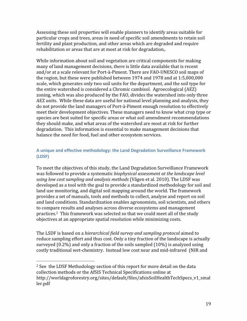
19
Assessing these soil properties will enable planners to identify areas suitable for particular crops and trees, areas in need of specific soil amendments to retain soil fertility and plant production, and other areas which are degraded and require rehabilitation or areas that are at most at risk for degradation,. While information about soil and vegetation are critical components for making many of land management decisions, there is little data available that is recent and/or at a scale relevant for Port-‐à-‐Piment. There are FAO-‐UNESCO soil maps of the region, but these were published between 1974 and 1978 and at 1:5,000,000 scale, which generates only two soil units for the department, and the soil type for the entire watershed is considered a Chromic cambisol. Agroecological (AEZ) zoning, which was also produced by the FAO, divides the watershed into only three AEZ units. While these data are useful for national level planning and analysis, they do not provide the land managers of Port-‐à-‐Piment enough resolution to effectively meet their development objectives. These managers need to know what crop type or species are best suited for specific areas or what soil amendment recommendations they should make, and what areas of the watershed are most at risk for further degradation. This information is essential to make management decisions that balance the need for food, fuel and other ecosystem services.
A unique and effective methodology: the Land Degradation Surveillance Framework (LDSF) To meet the objectives of this study, the Land Degradation Surveillance Framework was followed to provide a systematic biophysical assessment at the landscape level using low cost sampling and analysis methods (Vågen et al. 2010). The LDSF was developed as a tool with the goal to provide a standardized methodology for soil and land use monitoring, and digital soil mapping around the world. The framework provides a set of manuals, tools and methods to collect, analyze and report on soil and land conditions. Standardization enables agronomists, soil scientists, and others to compare results and analyses across diverse ecosystems and management practices.2 This framework was selected so that we could meet all of the study objectives at an appropriate spatial resolution while minimizing costs. The LSDF is based on a hierarchical field survey and sampling protocol aimed to reduce sampling effort and thus cost. Only a tiny fraction of the landscape is actually surveyed (0.2%) and only a fraction of the soils sampled (10%) is analyzed using costly traditional wet-‐chemistry. Instead low cost near and mid-‐infrared (NIR and
2 See the LDSF Methodology section of this report for more detail on the data collection methods or the AfSIS Technical Specifications online at http://worldagroforestry.org/sites/default/files/afsisSoilHealthTechSpecs_v1_smaller.pdf

20
MIR) diffuse spectroscopy are utilized to obtain spectral signatures of all the soil sampled (Stenberg et al. 2010). These spectra are used to predict physical and chemical values for all the soil samples. Geospatial statistics are then applied to extrapolate these results for the entire landscape. This analysis produces a suite of indicators of soil and vegetation that are spatially specific and continuous across the surveyed landscape. Maps of indicators can be used to assess overall landscape conditions. These conditions can be either compared within the landscape to identify areas of high and low values or over time to observe changes at any given point in the landscape. Indicators of landscape condition include observations of vegetation, topography, land management, and some soil physical properties (Table 1, page 17). Soil analysis produces indicators of soil chemical and physical properties (Table 2, page 20); together, these plant and vegetation analyses can be combined to provide site-‐specific indices of landscape health.
Enabling Land Use Planning and Analysis in the Port-‐à-‐Piment Watershed Land use management in agricultural landscapes can include a diversity of decision makers. In the Port-‐à-‐Piment watershed, these include farmers, non-‐governmental organizations, business owners, universities and government. This report was prepared to provide these stakeholders with information for the planning and development of the Cote Sud Initiative (CSI), a large multi-‐party development project spearheaded by the United Nations Environment Programme (UNEP) designed to help reach the Millennium Development Goals in the region. While the CSI is an integrated development project aiming to impact 10 communes in the South Department, the project is focusing much of its initial effort on developing a Millennium Village (MV) in Port-‐à-‐Piment. The Landscape Baseline Assessment was launched in order to provide MV project managers with immediate decision support tools including maps of key watershed and ecosystem health indicators, site specific information on crop and tree production requirement and limitations, and an associated land management decision framework. These tools were designed to help meet project goals by informing the implementation of interventions in the most strategic way. The specific development objectives and interventions that this analysis informs and agreed to in the initial project workplan: Development Objective 1: Reduce Hunger and Malnutrition
• Improve crop yields • Target and make efficient use of essential inputs • Maximize irrigation potential • Provide education, training, and extension
Development Objective 2: Improved Livelihoods
• Increase farm income
Development Objective 6: Improve the sustainability of the watershed

21
• Reduce soil erosion o Stabilize current landslides o Protect waterways o Promote cropping of appropriate plants based on slope and soil type o Establish grazing management plans
• Sustain wood products o Develop forestry management plans
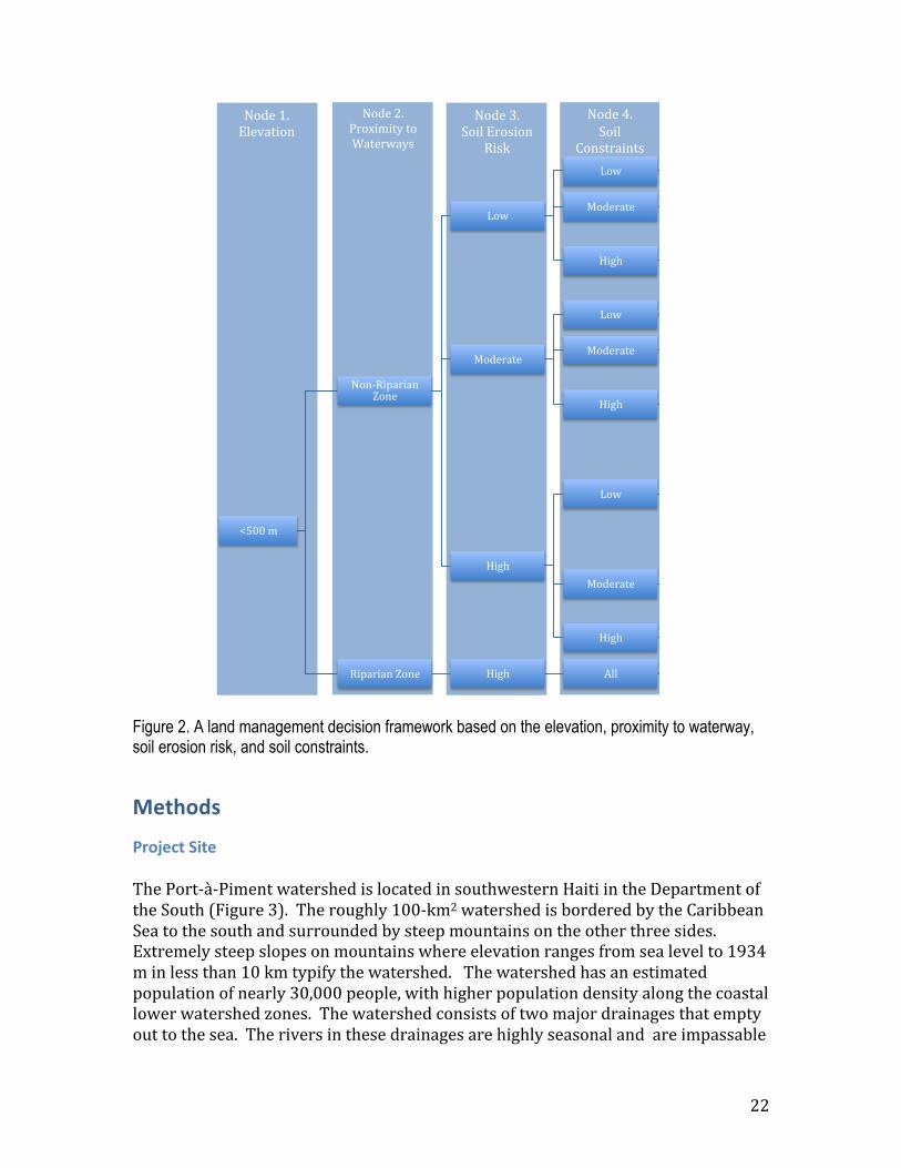
• Generate incentives for improving ecosystem services In order to meet these development objectives, project managers have a number of decisions to make as to what, how and where interventions are targeted (Figure 2). Basic land management decisions include whether to grow crops, graze animals, plant trees, and whether to actively rehabilitate the land or to not intervene at all and abandon it. The decision framework developed (Figure 2) and described later in this report can be used with or without the detailed data presented in this report for assisting in improving land management. The decision framework is based on a set of key questions related to the elevation, proximity to waterway, risk of erosion and potential soil constraints for any given piece of land. Answers to this set of hierarchical questions provide a guide for determining management recommendations (see Major Findings, Recommendations and Next Steps for a detailed description of the decision framework). Ideally, these decisions are made with information that accurately represents the socio-‐economic and biophysical situation in the project area and are made in direct consultation with the stakeholders that will be involved. Examples of the application of this decision framework with the Port-‐à-‐Piment Landscape Baseline Assessment data are illustrated in this report.
22
Figure 2. A land management decision framework based on the elevation, proximity to waterway, soil erosion risk, and soil constraints.
Methods
Project Site The Port-‐à-‐Piment watershed is located in southwestern Haiti in the Department of the South (Figure 3). The roughly 100-‐km2 watershed is bordered by the Caribbean Sea to the south and surrounded by steep mountains on the other three sides. Extremely steep slopes on mountains where elevation ranges from sea level to 1934 m in less than 10 km typify the watershed. The watershed has an estimated population of nearly 30,000 people, with higher population density along the coastal lower watershed zones. The watershed consists of two major drainages that empty out to the sea. The rivers in these drainages are highly seasonal and are impassable
!"#$%&'%()"*+,+-.%-"%/0-$)10.2%
!"#$%3'%4"+5%6)"2+"7%
8+29%
!"#$%:'%%4"+5%
;"72-)0+7-2%
()"#<=-+"7%()+")+-+$2%
4"+5%>070?$,$7-%
!"#$%@'%65$A0-+"7%
%
BCDD%,%
!"7E8+F0)+07%G"7$%
H"1%
H"1% ;)"FF+7?%@I&I3% J$)-I%K4J>LI%ML%
>"#$)0-$% ;)"FF+7?%@I&I3% J$)-I%K4J>I%M%
N+?O%(02-<)$%@ %%
($)$77+052%@%%
>"#$)0-$%
H"1% ;)"FF+7?%&I3% 4;I%J$)-I%K4J>I%M%
>"#$)0-$% ;)"FF+7?%&I3% 4;I%J$)-I%K4J>I%M%
N+?O%(02-<)$%@%
($)$77+052%@%
N+?O%
H"1%
;)"FF+7?%3% 4;I%K4J>I%M%
(02-<)$%@%
($)$77+052%@%
>"#$)0-$%(02-<)$%@%
($)$77+052%@%
N+?O% 8$?$7$)0-+"7%
8+F0)+07%G"7$% N+?O% M55% ($)$77+052%&%
23
during some periods of the rainy season, while at other times of the year are reduced to streams.
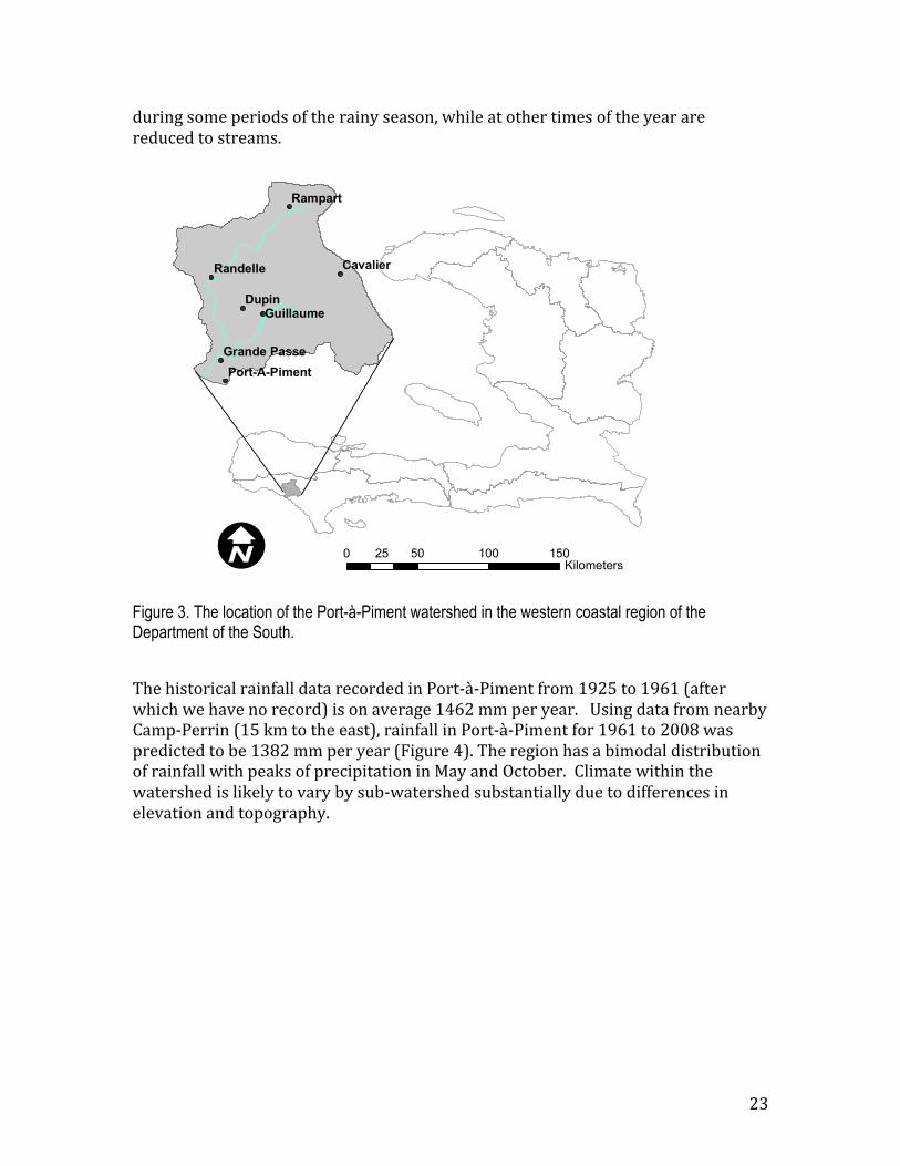
Figure 3. The location of the Port-à-Piment watershed in the western coastal region of the Department of the South.
The historical rainfall data recorded in Port-‐à-‐Piment from 1925 to 1961 (after which we have no record) is on average 1462 mm per year. Using data from nearby Camp-‐Perrin (15 km to the east), rainfall in Port-‐à-‐Piment for 1961 to 2008 was predicted to be 1382 mm per year (Figure 4). The region has a bimodal distribution of rainfall with peaks of precipitation in May and October. Climate within the watershed is likely to vary by sub-‐watershed substantially due to differences in elevation and topography.
Dupin
Rampart
CavalierRandelle
Guillaume
Grande PassePort-A-Piment
0 50 100 15025KilometersI

24
Figure 4. Mean monthly rainfall (mm) at Camp-Perrin from 1925 to 2008, Port-à-Piment from 1925-1961, and extrapolated values for Port-à-Piment 1962-2008.
LDSF Methodology
Field Methods3 The LDSF methodology utilizes a hierarchical sampling strategy based on a multilevel statistical framework that accounts for (scale specific) spatial variation. This statistical framework enables scaling of results from plot level, to landscape (Figure 5). The basic sampling frame, or block, a 100 km2 area (10 x 10 km) was divided into 16 equally sized clusters. Within each cluster 10 plots were randomly selected. Each of the 160 plots was subdivided into 4 subplots, one in the center of the plot and the three others surrounding the center plot, disposed at 120 degrees. Each plot has a 17.84 meters (m) radius (an area of 0.1 ha) and each subplot has a 5.64 m radius (an area of 0.01 ha) with its center 12.2 m away from the plot’s center. Observations and soil samples were taken from each plot. Basic characteristics of the entire plot were observed and recorded: landscape position, major land form, slope, current land management, land management history (if a land manager, e.g. farmer, was present and could provide information), evidence of flooding, existence
3 For a complete description of the LDSF field methodology please refer to the AfSIS Technical Specifications online at: http://worldagroforestry.org/sites/default/files/afsisSoilHealthTechSpecs_v1_smaller.pdf
!"
#!"
$!!"
$#!"
%!!"
%#!"
&!!"
&#!"
'!!"
'#!"
#!!"
()*+),-"
./0,+),-"
1),23"
45,67"
1)-"
(+*/"
(+7-"
4+8+9:"
;/5:/<0/,"
=2:>0/,"
?>@/<0/,"
A/2/<0/,"
!"#$%!&$
'()*%+#,$-#))%.//0%
B)<5CD/,,6*"$E%#C$EF$"
B)<5CD/,,6*"$EF$C%!!G"
D>,:CHCD6</*:"$E%#C$EF$"
D>,:CHCD6</*:"$EF%C%!!G"
25
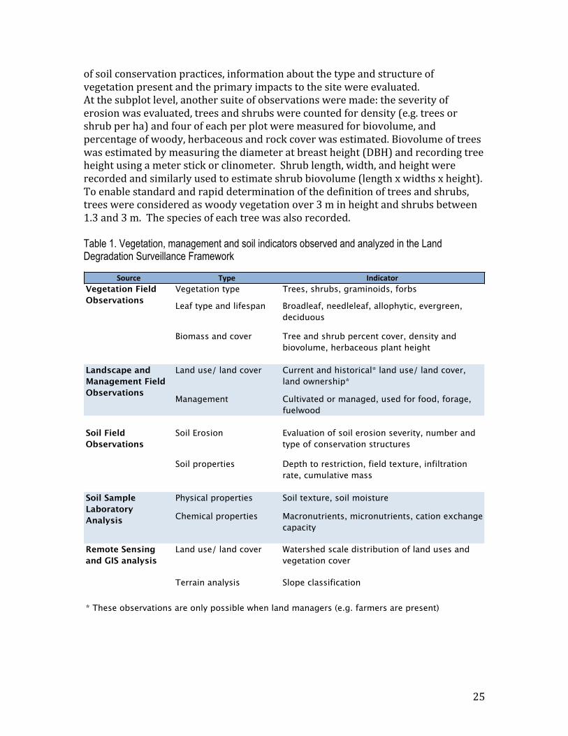
of soil conservation practices, information about the type and structure of vegetation present and the primary impacts to the site were evaluated. At the subplot level, another suite of observations were made: the severity of erosion was evaluated, trees and shrubs were counted for density (e.g. trees or shrub per ha) and four of each per plot were measured for biovolume, and percentage of woody, herbaceous and rock cover was estimated. Biovolume of trees was estimated by measuring the diameter at breast height (DBH) and recording tree height using a meter stick or clinometer. Shrub length, width, and height were recorded and similarly used to estimate shrub biovolume (length x widths x height). To enable standard and rapid determination of the definition of trees and shrubs, trees were considered as woody vegetation over 3 m in height and shrubs between 1.3 and 3 m. The species of each tree was also recorded. Table 1. Vegetation, management and soil indicators observed and analyzed in the Land Degradation Surveillance Framework
!"#$%& '()& *+,-%./"$Vegetation type Trees, shrubs, graminoids, forbs
Leaf type and lifespan Broadleaf, needleleaf, allophytic, evergreen, deciduous
Biomass and cover Tree and shrub percent cover, density and biovolume, herbaceous plant height
Land use/ land cover Current and historical* land use/ land cover, land ownership*
Management Cultivated or managed, used for food, forage, fuelwood
Soil Erosion Evaluation of soil erosion severity, number and type of conservation structures
Soil properties Depth to restriction, field texture, infiltration rate, cumulative mass
Physical properties Soil texture, soil moisture
Chemical properties Macronutrients, micronutrients, cation exchange capacity
Remote Sensing and GIS analysis
Land use/ land cover Watershed scale distribution of land uses and vegetation cover
Terrain analysis Slope classification
* These observations are only possible when land managers (e.g. farmers are present)
Landscape and Management Field Observations
Vegetation Field Observations
Soil Field Observations
Soil Sample Laboratory Analysis

26
Figure 5. The LDSF method utilizes a hierarchical sampling strategy that enables a statistically robust extrapolation from the subplot and plot to the landscape.
Infiltration. Water infiltration rates were measured in three plots per cluster, selected randomly from the ten plots in each cluster (Vågen et al. 2010). At the center of each of these plots, a 12-‐inch diameter single-‐ring infiltrometer was pounded vertically into the soil surface to a depth of at least 5 cm and the soil around the ring was packed to prevent leakage. Any vegetation, litter, or large rocks were carefully removed by cutting at the soil surface from inside the ring to prevent disturbing the soil surface. The soil was pre-‐wetted, by pouring 2-‐3 liters of water into the ring and was allowed to soak into the soil for 15-‐20 minutes. Then water was added to a 20 cm depth of the ring, and the depth of water was recorded every 5 minutes or until the water level dropped to zero (falling-‐head technique). Water was refilled to 20 cm as necessary to ensure that infiltration depths had been recorded for at least 1 hour. Infiltration capacity was estimated using Horton’s equation:
Where ft is the infiltration rate at time t, f0 is the initial infiltration rate (maximum), fc is the constant or equilibrium infiltration rate, and k is the decay constant specific to that soil. The model was implemented using nonlinear mixed effects (nlme)
!(
!(!(!(!(
!(!(
!(!(!(!(!(
!(!(!(!( !(
!(
!(
!(!(
!(!(
!(
!(!(
!(!(
!(!(
!(!(!(!(!(
!(!(!(!(!(!(!(!(
!(!(
!(!(
!(!(!(!(!(!(!(!(
!(
!(!(!(!(!(!(!(!(
!(!(
!(!(
!(!(!(!(
!(!( !(!(!(!( !(!(!(!(
!(!(
!(!(!(!(!(!(!(
!(!(!(!(!(!(
!(!(!(!(!(!(
!(!(
!(!(!(!(
!(!(
!(!(!(!(!(!(
!(!(!(!(!(!(
!(!(!(!(
!(!(!(!(
!(!(!(!(
!(!(!(
!(!(!(!(
!(!(!(!(!(!(!(
!(!(
!(!(!(!(
!(!(!(!(!(
!(!(
!(!(
!(!(
!(!(!(!(!(!(
!(!(!(!(
!(!(
!(
!(!(!(!(
!(!(!(!(!(!(!(!( !(!(
!(!(!(!(!(!(
!(!(
!(!(
!(!(
!(!(!(!( !(!(!(!(!(!(!(!(
!(!(
!(!(!(!(!(!(!(!(!(!(
!(!(
!(!(
!(!(!(
!(
!(!(!(!(
!(!(!(!(!(!(!(!(!(!(!(
!(!(
!(!(!(!(!(
!(!(!(!(
!(!(!(!(!(!(
!(!( !(!(!(!(
!(!(
!(!(
!(!(!(!(
Rivers
!( LDSF plots
0 2,000 4,000 6,0001,000MetersI
Block level: Each block is a 10x10 km square divided into a grid composed of 16 clusters
Cluster level: Each cluster has 10 randomly selected plots
Plot level: Each 0.1 ha plot consists of four 0.01 ha subplots
ft = fc + (f0 – fc)e-‐kt

27
model in R. This selfStart model evaluates the asymptotic regression function and solves for fc, f0, and k with water depth and time as the input parameters. We report infiltration rates (fc) in mm/hour.
Soil sampling. In the center of each of the four subplots, soil samples were taken at two depths (0-‐20 cm and 20-‐50 cm) and composited for each soil depth in buckets, thoroughly homogenized, sub-‐sampled and bagged for transport back to the laboratory. After the samples were taken from each subplot, holes were augered to a depth of 100 cm if possible. If not possible, the depth to restriction was recorded.
Lab methods Soil physical and chemical analysis. Sub-‐samples (~100 g) were taken, weighed, dried for 48 hours at 105 °C and re-‐weighed to determine gravimetric soil moisture. Soils were air-‐dried for one week, sieved to 2mm and then ground for analysis. Sieved soil samples (~400 g) and ground subsamples (for infrared spectroscopy ~20 g) were then sent to the World Agroforestry Centre (ICRAF) Soil-‐Plant Spectral Diagnostics Laboratory facility in Nairobi, Kenya and the Natural Resource Conservation Service (NRCS) Laboratory in Lincoln, Nebraska in the United States. Both of these laboratories are leading the development of near (NIR) and mid-‐infrared (MIR) diffuse reflectance spectroscopy for soil analysis. The NIR (1,250 nm to 2,500 nm) spectral analysis was done with a Bruker Fourier-‐Transform MultiPurpose Analyzer spectrometers (MPA), manufactured by Bruker Optik GmbH, Germany) and the MIR (2,500 to 25,000 nm) with a Bruker Tensor 27 Fourier-‐Transform spectrometer attached to a High-‐Throughput Screening (HTS-‐XT) accessory. All soils samples were analyzed using NIR and MIR spectroscopy (Brown et al 2006). Ten percent of the soil samples collected were also analyzed using traditional wet chemistry analysis. The wet chemistry results and field data were used to develop a partial least squares model to predict the physical and chemical properties (Table 2) of the other 90% of the soil samples.

28
Table 2. Soil physical and chemical indicators from the LDSF and their importance for agricultural productions (Brady and Weil 2002, Fageria 2009; Lindsay 1972).
!"#$%&'(#)*+",% -"$.%#'%/$*'+%0,"1+2344.'+#*$%5$*'+%6*),"'7+,#.'+4!"#$%&'()!"* !"#$%&'(%+(,%-"#(./0($1##(21.13+1+4(5"631+%&'()56* 5"631+%&'($/3-0%7&-1+(-/(,"0%/&+(8#"3-('1-"7/#%$("$-%,%-9(%3$#&2%36(8:/-/+93-:1+%+;/-"#(<%-0/613()<* (=3$01"+1(8#"3-(80/2&$-%,%-9(79($/3-0%7&-%36(-/("##("'%3/("$%2+>(3&$#1%$("$%2+("32($:#/0/8:9##4
?:/+8:/0&+()?* ?:/+8:/0&+(%+(01@&%012(79A(8:/-/+93-:1+%+>(3%-0/613(.%B"-%/3>(.#/C10%36>(.0&%-%36("32('"-&0"-%/34(
?/-"++%&'()D* (?/-"++%&'(8#"9+("3(%'8/0-"3-(0/#1(%3(01-"%3%36(C"-10("32(%3(2%..1013-('1-"7/#%+'+(%3$#&2%36(8:/-/+93-:1+%+>(80/-1%3(+93-:1+%+>(3%-0/613(.%B"-%/3>(+-"0$:(./0'"-%/3("32(-:1(-0"3+#/$"-%/3(/.(+&6"04
E&#.&0()E* E&#.&0(:1#8+($/3-0/#(3%-0/613($"8-&01("32(-:1(8:/-/+93-:1+%+(80/$1++4
344.'+#*$%5$*'+%6#),"'7+,#.'+4F/0/3(()F* F/0/3(%+("3(%'8/0-"3-(1#1'13-(/.($1##&#"0(2%,%+%/3("32(60/C-:4!/8810()!&* G3(1++13-%"#($/'8/313-(/.('/+-(7%/$:1'%$"#(80/$1++1+4(=-(13:"3$1+(8:/-/+93-:1+%+>(
3%-0/613(.%B"-%/3>(.#/C10%36>(.0&%-%36("32('"-&0"-%/34(=0/3()H1* (=0/3(%+(01@&%012(%3($:#/0/8:9##(+93-:1+%+45"36"31+1()53* ?:/-/+93-:1+%+("32(3%-0/613('1-/7/#%$("$-%,%-9("01(21813213-(/3(5"36"31+14I%3$()I3* I%3$(21.%$%13$9(012&$1+(8#"3-(60/C-:("32(01+&#-+(%3(+-&3-%36>(%3-103/2"#(+:/0-13%36>(
%3-10,1%3"#($:#/0/+%+(/3(#1",1+>("32(,109(/.-13(9%1#2(012&$-%/3+(./&32(J%3$(21.%$%13$9(3/-(K&+-(2&1(-/(#/C(#1,1#+(%3(8"013-('"-10%"#>(7&-("#+/(2&1(-/("7+/08-%/3(/.(-:1(3&-0%13-(79(+/%#($/##/%2+(%3(:%6:(8L(+/%#+4
8+2.,%9.:%;2.<#)*$%&'(#)*+",4MB$:"361"7#1(G#&'%3&'()G#* MB$:"361"7#1(G#(+-0/36#9($/3-0/#+(+/%#("$%2%-9("32(0//-(60/C-:(71#/C(8L(N4N4
E/%#("$%2%-9()8L* E/%#("$%2%-9(%+(2%01$-#9(01#"-12(-/(-:1("7%#%-9(/.(0//-+(-/(-"O1(%3(+1,10"#(1#1'13-+(%3(-:1(+/%#(%3$#&2%36(3&-0%13-+("32(-/B%3+4(=-("#+/(8#"9+("(0/#1(%3(-:1(0"-1(/.(21$"9(/.(8/##&-"3-+4
E/%#(P06"3%$(!"07/3()EP!* E/%#(P06"3%$(!"07/3(01801+13-+("(#"061(01+10,1(/.(3&-0%13-+>(%3$01"+1+($"-%/3(1B$:"361($"8"$%-9>(012&$1+(3&-0%13-(#1"$:%36>($/3-0%7&-1+(-/(+/%#(+-0&$-&01>(%'80/,1+(%3.%#-0"-%/3>(%3$01"+1+(-:1(8/-13-%"#(./0(+/%#(-/(:/#2(C"-10("32(%'80/,1+(-:1(+/%#+($"8"$%-9(-/(7&..10($:"361+(%3(8L4
!"-%/3(1B$:"361($"8"$%-9()!M!* ;:1(+&'(/.(-:1(-/-"#(/.(-:1(1B$:"361"7#1($"-%/3+(-:"-($"3(71("7+/0712(79(-:1(+/%#4(Q+12(-/("++1++(-:1(","%#"7%#%-9(/.(3&-0%13-+(./0(8#"3-(60/C-:("32(801+$0%71(+/%#("'132'13-+4
!"#$%&'(-/(5"631+%&'(0"-%/()!"A56*
;:1(0"-%/(%+(&+12(-/(801+$0%71(+/%#("'132'13-+4
M#1$-0%$"#(!/32&$-%,%-9()M!* =+("('1"+&01(/.(+"#%3%-94((L%6:(+"#-($/3$13-0"-%/3+(%3(-:1(+/%#($"3(316"-%,1#9("..1$-(8#"3-(60/C-:4(
52:4#)*$%&'(#)*+",4!&'&#"-%,1('"++ ;:1($&'&#"-%,1(+/%#(80/810-9($/3-13-()1464(+/%#($"07/3*(810(&3%-(60/&32("01"(-/(-:1(-"061-(
209(+/%#('"++(810(&3%-(60/&32("01"4(G('1"3+(/.("$$&0"-1#9(1B-0"8/#"-%36((-:1(3&-0%13-($/3$13-0"-%/3+(/.("(+/%#(+"'8#1(-/(-:1(218-:(/.(-:1(+/%#4(((
;1B-&01 ;1B-&01()-:1("'/&3-+(/.(+"32>(+%#->("32($#"9*(%+(%3,/#,12(%3(21-10'%3%36('"39(/.(-:1(+/%#(8:9+%$"#("32($:1'%$"#(80/810-%1+(/.(+/%#+>(%3$#&2%36(C"-10('/,1'13->(C"-10(:/#2%36($"8"$%-9>(3&-0%13-(7&..10%36($"8"$%-94
=3.%#-0"-%/3(0"-1 ;:1(0"-1(-:1(C"-10(%3.%#-0"-1+(%3-/(-:1(+/%#(%32%$"-1+(:/C('&$:(C"-10('"9(71(","%#"7#1(-/(8#"3-+>(%+(01$:"06%36(60/&32(C"-10(+/&0$1+("32(:/C('&$:(%+(8/32%36(/0(0&33%36("$0/++(-:1(+&0."$14
E#/81 E#/81(%3($/'7%3"-%/3(C%-:(+/%#(8:9+%$"#(80/810-%1+(21-10'%31+(0&3/..("32(10/+%/3(0"-1+4
29
Soil mapping Soil properties measured and estimated from the LSDF procedures were analyzed to produce digital maps to enable a better understanding of the soil conditions across the watershed. The specific objectives of these analyses were to predict soil physical and chemical values for the watershed as well as to predict the probability of exceeding certain values determined to be critical for plant growth (Shepherd 2011). Using a geospatial statistical method called co-‐kriging, soil properties reported for each plot were used to predict values for all of the area of the watershed where the soil was not sampled. Geospatial statistics are based on an assumption that data from points that are closer together spatially are more likely to be similar than those far apart. The analysis of the relationship of the variation of the data and the distance between the points where it was collected enables predictions based on distance. The development of soils and their properties is extremely complex, however, and variation due to spatial location alone is unlikely to explain or predict their status well -‐-‐ including the factors that control soil formation can help build better predictive models. This approach of including other factors (co-‐variates) in digital soil mapping has been formalized as SCORPAN by McBratney (McBratney 2003). Where:
• s: soil, other properties of the soil at a point;
• c: climate, climatic properties of the environment at a point;
• o: organisms, vegetation or fauna or human activity;
• r: topography, landscape attributes;
• p: parent material, lithology;
• a: age, the time factor;
• n: space, spatial position. The ArcGIS co-‐kriging process allows up to 3 covariates. For most of the maps generated a 30-‐m digital elevation model (DEM), and a slope grid derived from the DEM were used as covariates for the co-‐kriging analysis. For some specific cases, a vegetation co-‐variate was also used, this covariate was derived from 4 bands of orthorectified IKONOS® images and the three components (green, dark and bright) derived from Spectral Mixing Analysis (SMA) (Small 2004). The SMA was used to distinguish each pixel across the landscape based on their relative distribution of green, dark and bright spectra which corresponds to characteristics such as the amount of vegetation cover (i.e. more green) or water (i.e. dark). Modelling the spatial information and co-‐variates is done via an iterative process broken down in two stages using the ArcGIS Geostatistical Analyst tool (ESRI 2011)4: quantifying the
4 The ArcGIS Geostatistical Analyst documentation can be found online at: http://www.esri.com/software/arcgis/extensions/geostatistical/index.html
30
spatial structure of the data and producing a prediction. Co-‐kriging uses the fitted model from the spatial data configuration, and the soil property values from sampled points to make a prediction for the unknown values of the other location throughout the watershed that were not sampled. Maps that integrate multiple soil and vegetation measures were generated using ArcGIS’s raster math function.
Soil fertility constraints To provide an integrated assessment of the potential constraints to plant productivity due to soil chemistry each soil parameter was assessed base on a threshold values developed for the soil Fertility Capability Classification (FCC) (Sanchez 2003). The number of set thresholds (Appendix I) that were exceeded for each of the 19 soil chemistry parameters analyzed was then summed to produce an integrated map.
Soil erosion To estimate current soil losses across the landscape the revised universal soil loss equation (RUSLE) was used (Rahman et al. 2009). The RUSLE equation combines multiple biophysical data layers to estimate soil loss (A) as follows:
A = R × K × L × S × C × P Where: A = the soil loss in Mg ha−1 year−1; K = the soil erodibility factor Mg ha−1 MJ−1 mm−1; R = the rainfall-‐runoff erosivity factor in MJ mm ha−1 h−1 year−1; L = the slope length factor; S = the slope steepness factor; C = the cover and management factor and P = the conservation practices factor The K factor was calculated from the following equation (Lim et al. 2010): Equation 1: K-factor
0.2+ 0.3 × exp −0.0256 × !"#$ × 1− !"#$100
× 1.0− 0.25 ×!"#$
!"#$ + exp 3.72− 2.95 × !"#$
× 1.0− 0.7 ×!"1
!"1+ exp(−5.51+ 22.9 × !"1

31
Where, Sand is the percentage of sand (%), Silt is the percentage of silt (%), Clay is the percentage of clay (%), and SN1 is (1-‐Sand/100) predicted for each plot. The R factor was calculated using climate data from Camp Perrin 1993 to 2009 (ORE 2011) and the following equations (Renard and Freimund, 1994 in Rahman et al. 2009):
Equation 2: R factor
If F < 55!! !ℎ!" ! = 0.07397!!.!"#
1.72
If F ≥ 55mm then ! = 95.77− 6.081! + 0.4770!!
17.2
Where ! = !!!!"
!!!
!"!"!!!
and Pi is the monthly rainfall in mm
and F is the modified Fournier coefficient. The L and S factors were estimated using the ArcGIS routines outlined by Mitasova et al. (Mitasova and Brown 2012). For each of the land use land cover classifications a C factor was adapted using documentation provided for the RUSLE2 model (NRCS 2006). The P factor was assumed to be 1 for all land uses, since no conservation practices had been observed.
Table 3. Recommended slope limits (%slope) for agricultural management practices based on input intensity (FAO 1993)
Land use land cover classifications and terrain analysis We analyzed the terrain of the watershed using the Slope function in the Spatial Analyst module of ArcGIS 10 (ESRI 2011) with a 30m digital elevation model (DEM) as our input data. Slopes were then parsed into three major classes, level, 0 to 16%;
!"# $%&'()'*+,&' -+./!"#$%&'()*+,-(.#/0+1/(-+#2()+$-&*3"/#+$(4&"-1*&-( 567 567 589!"#$%&'()*+,-(.#/0(-+#2()+$-&*3"/#+$(4&"-1*&-( 567 567 567:**#;"/&'()*+,-(.#/0+1/(-+#2()+$-&*3"/#+$(4&"-1*&-( 5< 5< 5=:**#;"/&'()*+,-(.#/0(-+#2()+$-&*3"/#+$(4&"-1*&->/&**")#$;? 567 567 567@+%%&&A(/&"A(%1&2.++'("$'(,"-/1*&A(.#/0("$'(.#/0+1/(-+#2()+$-&*3"/#+$(4&"-1*&-
5B< 567 5B<
!,%*01'$%20&3$%&'%1+&4
32
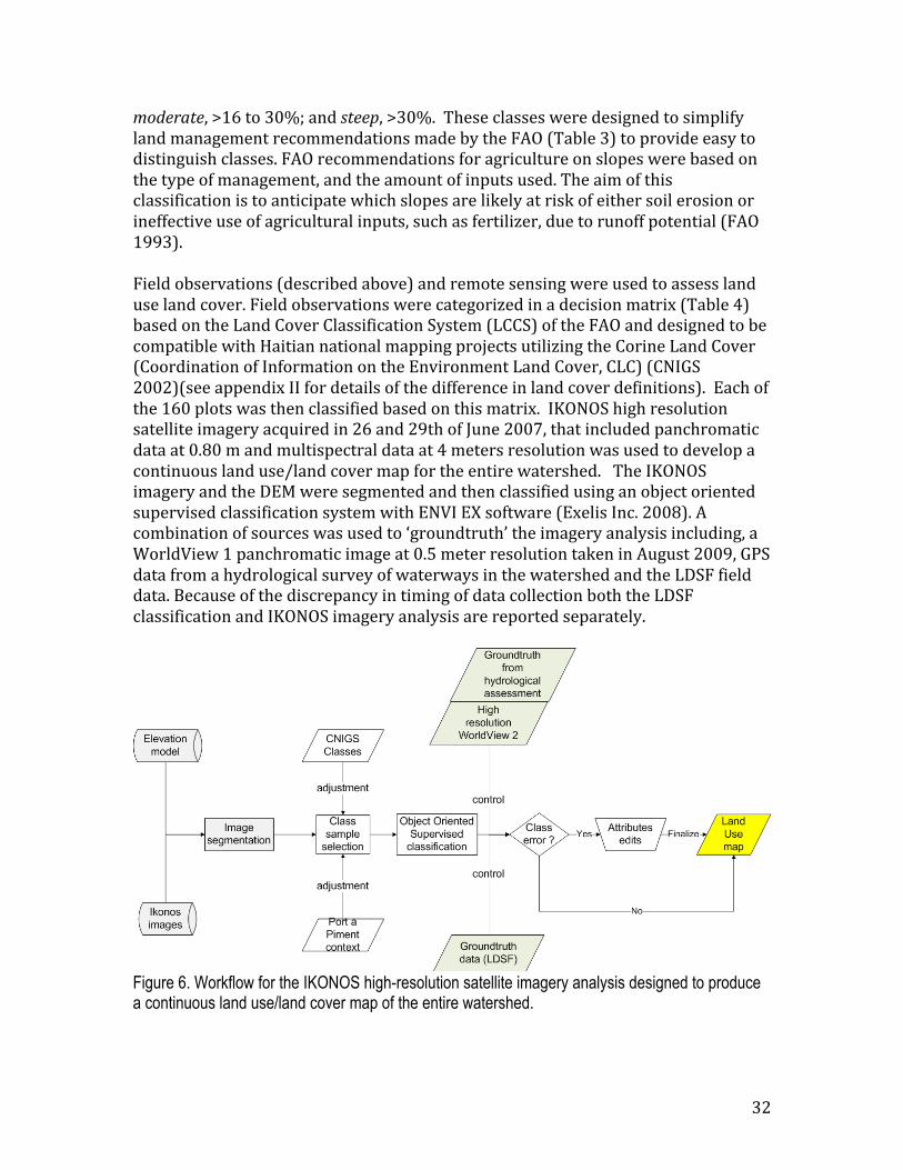
moderate, >16 to 30%; and steep, >30%. These classes were designed to simplify land management recommendations made by the FAO (Table 3) to provide easy to distinguish classes. FAO recommendations for agriculture on slopes were based on the type of management, and the amount of inputs used. The aim of this classification is to anticipate which slopes are likely at risk of either soil erosion or ineffective use of agricultural inputs, such as fertilizer, due to runoff potential (FAO 1993). Field observations (described above) and remote sensing were used to assess land use land cover. Field observations were categorized in a decision matrix (Table 4) based on the Land Cover Classification System (LCCS) of the FAO and designed to be compatible with Haitian national mapping projects utilizing the Corine Land Cover (Coordination of Information on the Environment Land Cover, CLC) (CNIGS 2002)(see appendix II for details of the difference in land cover definitions). Each of the 160 plots was then classified based on this matrix. IKONOS high resolution satellite imagery acquired in 26 and 29th of June 2007, that included panchromatic data at 0.80 m and multispectral data at 4 meters resolution was used to develop a continuous land use/land cover map for the entire watershed. The IKONOS imagery and the DEM were segmented and then classified using an object oriented supervised classification system with ENVI EX software (Exelis Inc. 2008). A combination of sources was used to ‘groundtruth’ the imagery analysis including, a WorldView 1 panchromatic image at 0.5 meter resolution taken in August 2009, GPS data from a hydrological survey of waterways in the watershed and the LDSF field data. Because of the discrepancy in timing of data collection both the LDSF classification and IKONOS imagery analysis are reported separately.
Figure 6. Workflow for the IKONOS high-resolution satellite imagery analysis designed to produce a continuous land use/land cover map of the entire watershed.
33
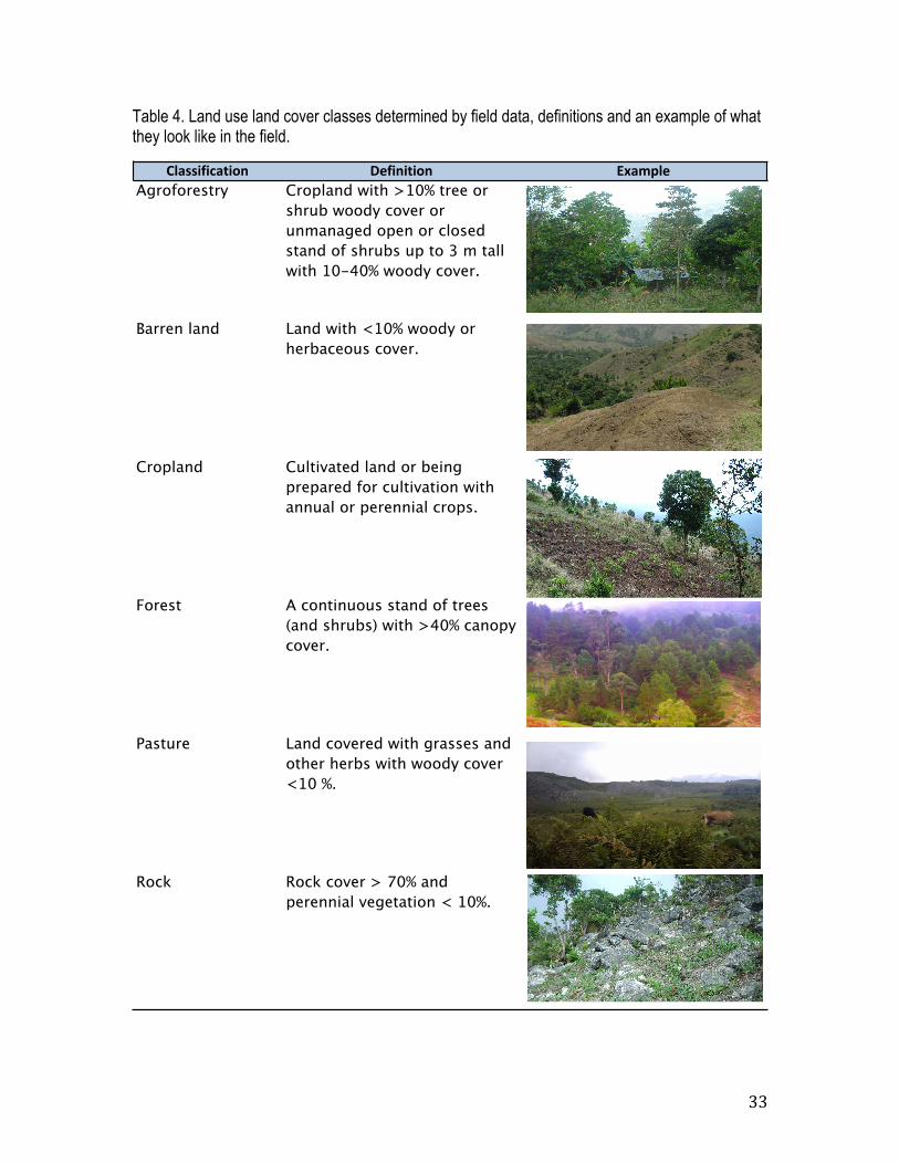
Table 4. Land use land cover classes determined by field data, definitions and an example of what they look like in the field.
!"#$$%&%'#(%)* +,&%*%(%)* -.#/0",1Agroforestry Cropland with >10% tree or
shrub woody cover or unmanaged open or closed stand of shrubs up to 3 m tall with 10-40% woody cover.
Barren land Land with <10% woody or herbaceous cover.
Cropland Cultivated land or being prepared for cultivation with annual or perennial crops.
Forest A continuous stand of trees (and shrubs) with >40% canopy cover.
Pasture Land covered with grasses and other herbs with woody cover <10 %.
Rock Rock cover > 70% and perennial vegetation < 10%.
34
Statistical analysis We performed linear mixed-‐models to compare differences in soil and vegetation results by land use/land cover, elevation and slope classifications using cluster as a random effect. A likelihood ratio test was used to compare the full model with the reduced model to determine if the model is adequate. For models that were significant we then assessed differences between pairs using Tukey’s Honestly Significant Difference. Univariate regression of infiltration capacity as a function of tree density (in trees/ha) was assessed by blocking by cluster to account for spatial variability. We also used a linear mixed-‐model to compare tree density categories: low (0-‐100 trees/ha), mid (100-‐300 trees/ha), and high (300+ trees/ha) and the effect of land cover class on infiltration capacity. Partial least squares (PLS) regression, was used to predict soil properties for each spectra based on the wet chemistry analysis. PLS is a type of multivariate analysis that has few analysis restrictions and is thus highly flexible, and can be employed in situations where more traditional analysis methods are limited. All statistical analyses were run using the open source software R (R Development Core Team 2008).

35
Results and Discussion
Landscape Characteristics, Use and Cover
Field observations provided data for analysis of landscape characteristics, LULC, vegetation status, soil properties and incidence of erosion. While some parts of the study area showed clear signs of degradation others suggest a fairly productive agricultural system. We illustrate here how these indicators differed by visually distinguishing characteristics, LULC classes, and/or by elevation and slope depending on whether there were statistical differences. Key baseline values are highlighted, recommendations provided when appropriate and 5-‐year targets when possible are suggested.
Slope The area of the watershed with relatively flat land available for farmers to grow their crops on is extremely limited. The vast majority (>64%) of the landscape is considered steep slopes or slopes that are >30% (Table 5, Figure 7). Moderate slopes, which make up 23% of the watershed, still may have some risk of soil and nutrient losses without conservation measures. Level slopes are not likely to be at risk of soil erosion due to runoff regardless of the inputs but make up only 14% of the total area. The level area in the lower watershed (below 500 m), or flat lowlands, is where agriculture is most likely to be most productive. This area, which is primarily riparian bench, largely consists of settlements, some irrigated agriculture and agroforestry plantations.
Baseline: • 88% of the watershed is some type of agricultural production, annual
cropping, agroforestry or pasture • 45% of steep slopes are in annual cropping • 11% of steep slope are pasture • Only 5% of the landscape is covered in forests • Only 12% of the area on steep slopes was covered by woody plants (trees
and shrubs) Recommendation: • Promote agroforestry, reforestation, forest protection and vegetative soil
conservation practices on steep slopes • Promote high density short rotation woodfuel plantations
Target: • Increase forest cover on steep slopes to 10% and woody cover to 20% • Covert all of annual cropping and pasture on steep slopes to agroforestry
or agrosilvopastoral systems.
36
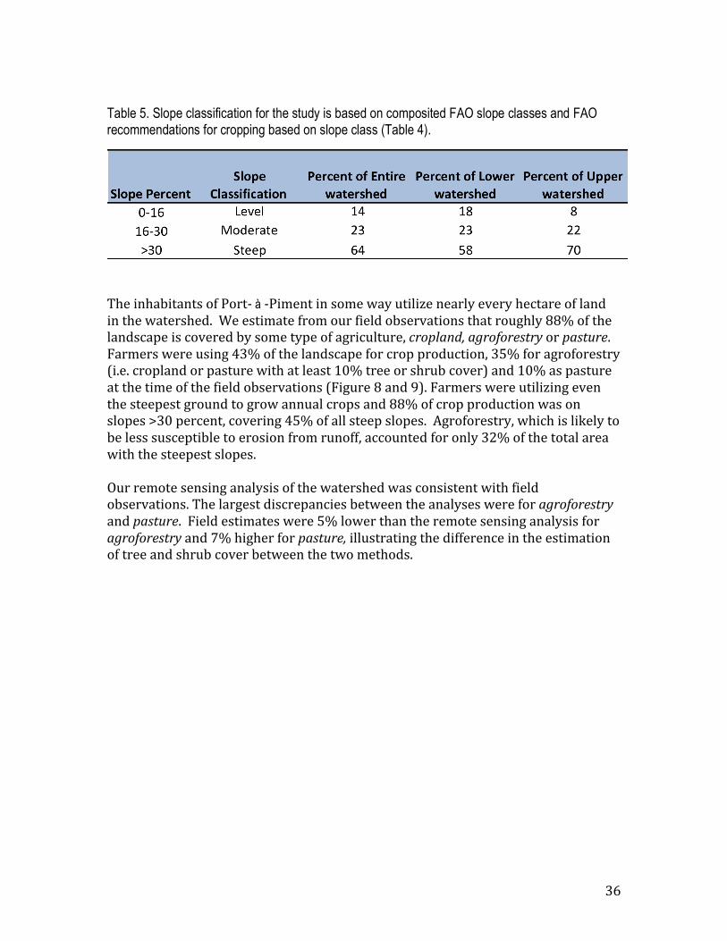
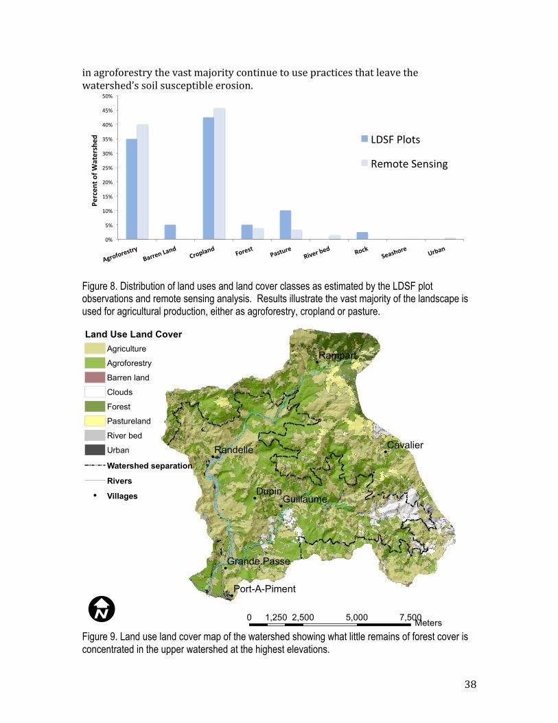
The inhabitants of Port-‐ à -‐Piment in some way utilize nearly every hectare of land in the watershed. We estimate from our field observations that roughly 88% of the landscape is covered by some type of agriculture, cropland, agroforestry or pasture. Farmers were using 43% of the landscape for crop production, 35% for agroforestry (i.e. cropland or pasture with at least 10% tree or shrub cover) and 10% as pasture at the time of the field observations (Figure 8 and 9). Farmers were utilizing even the steepest ground to grow annual crops and 88% of crop production was on slopes >30 percent, covering 45% of all steep slopes. Agroforestry, which is likely to be less susceptible to erosion from runoff, accounted for only 32% of the total area with the steepest slopes. Our remote sensing analysis of the watershed was consistent with field observations. The largest discrepancies between the analyses were for agroforestry and pasture. Field estimates were 5% lower than the remote sensing analysis for agroforestry and 7% higher for pasture, illustrating the difference in the estimation of tree and shrub cover between the two methods.
Table 5. Slope classification for the study is based on composited FAO slope classes and FAO recommendations for cropping based on slope class (Table 4).

37
Figure 7. Map illustrating the distribution of slope (in percent) for the watershed delineated (dashed line) into upper (>500 m) and lower watershed (<500 m).
As much of the land use is continuously changing depending on the time of year and even from year to year, the relative amount of cropland and pasture in particular should be assumed to be dynamic. The LDSF sampling method did not capture crop rotations and it is possible pasture could also be in crop production at another point in the year or even that barren land (5%) may be part of a rotation and could in the future be returned to crop production or pasture. We estimate that only 5% of the total landscape is under forest cover leaving most of the steepest highly erodible areas with no tree cover. Areas dominated by rocky outcroppings, or boulders (>70% rock cover) were only 3% of the total landscape. These areas often had some tree cover (< 10% woody cover) in the pockets of soil among the rocks. These pockets of soil in some cases were had soil > 50 cm and were used for agriculture (pasture or cropping) among the rocks.
Land Use /Land Cover The distribution of land use/land cover across the watershed illustrates a critical challenge for the sustainability of those who are reliant on the ecosystem services provided by this landscape for their livelihoods. The steep slopes that dominate the watershed are largely inappropriate for the annual cropping that is by far the most prevalent management practice. While some farmers have made an effort to engage
!
!
!
!
!
!
!
Dupin
Rampart
CavalierRandelle
Guillaume
Grande Passe
Port-A-Piment 0 2,000 4,000 6,0001,000Meters
I
Watershed SlopePercent
Level (0 - 16%)
Moderate (16 - 30%)
Steep (>30%)
Upper/Lower Delineation
Rivers
! Villages
38
in agroforestry the vast majority continue to use practices that leave the watershed’s soil susceptible erosion.
Figure 8. Distribution of land uses and land cover classes as estimated by the LDSF plot observations and remote sensing analysis. Results illustrate the vast majority of the landscape is used for agricultural production, either as agroforestry, cropland or pasture.
Figure 9. Land use land cover map of the watershed showing what little remains of forest cover is concentrated in the upper watershed at the highest elevations.
!"#
$"#
%!"#
%$"#
&!"#
&$"#
'!"#
'$"#
(!"#
($"#
$!"#
!"#$%$#&'
(#)*
+,##&-*.,-
/*0#$12
,-/* 3$#&'(*
4,'(5#&*
678&#*9&/* 6$:;
*<&,'=
$#&* >#9,-*
4&#:&-
(*$%*?
,(&#'=&/
*
)*+,#-./01#
234/03#+351657#
!
!
!
!
!
!
!
Dupin
Rampart
CavalierRandelle
Guillaume
Grande Passe
Port-A-Piment
0 2,500 5,000 7,5001,250 MetersI
Land Use Land CoverAgriculture
Agroforestry
Barren land
Clouds
Forest
Pastureland
River bed
Urban
Watershed separation
Rivers! Villages

39
Vegetation Much of the Port-‐à-‐Piment watershed was likely once covered by a dense canopy of trees or shrubs and that the upper watershed likely had vegetation similar to what is found in the Pic Macaya National Park to north. Most of this type of perennial vegetation has however been removed and replaced by annual cropping. Based on LDSF field plots, we estimated that only 14% of the landscape was still covered by woody plant species determined as the percent canopy coverage of trees and shrubs for each plot. The distribution of this woody cover was highly variable across the landscape and was significantly different among LULC classes but not between elevations or among slopes. In the upper watershed woody cover averaged 18% while in the lower watershed 10%. On the steepest slopes, most susceptible to erosion, woody coverage was on average only 12%, whereas on the moderate slopes coverage was 19%, and on the areas of the watershed where erosion risk is the lowest, coverage was actually the highest at 28% (Figure 10). On these steep slopes this situation is critical. Without woody cover, soil stabilization is reliant on the rooting systems of mainly annual crops. Inevitably there will be periods of the year when these crops will be harvested and the soil on these slopes bare and highly susceptible to wind and water erosion. The woody cover is primarily in agroforestry systems, a land use which averages 25% cover (Figure 11a). While woody cover on land in agroforestry was significantly higher (p<0.001) than that of cropland, pasture, barren land, or rock it was far lower than the relatively intact forests, which had on average 62% cover. There were, however, several observations of agroforestry systems that had woody cover equivalent to or greater than that of the average forest cover, indicating the potential to maintain protective woody cover while engaging in agricultural production. Tree density across the landscape was on average 456 trees ha-‐1. The median however was much lower 212 trees ha-‐1 which indicates there were high densities (number per ha) in some areas while majority of the landscape was largely treeless (Figure 11b). As with woody cover, there were significant differences in tree density among LULC classes (p<0.0001); mean tree density was highest for forests with 3172 trees ha-‐1 followed by agroforestry and rock with 547 and 350 trees ha-‐1 respectively. Mean tree density for cropland was 207 trees ha-‐1, pasture, 73
Figure 10. Box plots illustrating the lower quartile (Q1), median (Q2), upper quartile (Q3), and extreme values (dots) of percent woody cover by slope
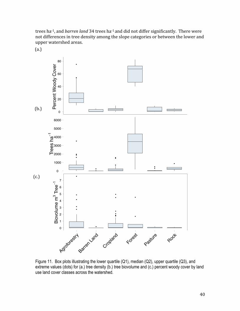
40
Biov
olum
e m
3 Tre
e!1
0
1
2
3
4
5
6
7
!
!
!
!
!
!
!
!
!
!!
!
!
!
!
Agrofor
estry
Barren
Land
Croplan
dFo
rest
Pastur
eRoc
k
Perc
ent W
oody
Cov
er
0
20
40
60
80!
!!
Agrofor
estry
Barren
Land
Croplan
dFo
rest
Pastur
eRoc
k
Tree
s ha
!1
0
1000
2000
3000
4000
5000
6000
!
!!
!
!
!
!
!!
!
!
!
Agrofor
estry
Barren
Land
Croplan
dFo
rest
Pastur
eRoc
k
trees ha-‐1, and barren land 34 trees ha-‐1 and did not differ significantly. There were not differences in tree density among the slope categories or between the lower and upper watershed areas.
Figure 11. Box plots illustrating the lower quartile (Q1), median (Q2), upper quartile (Q3), and extreme values (dots) for (a.) tree density (b.) tree biovolume and (c.) percent woody cover by land use land cover classes across the watershed.
(a.)
(b.)
(c.)
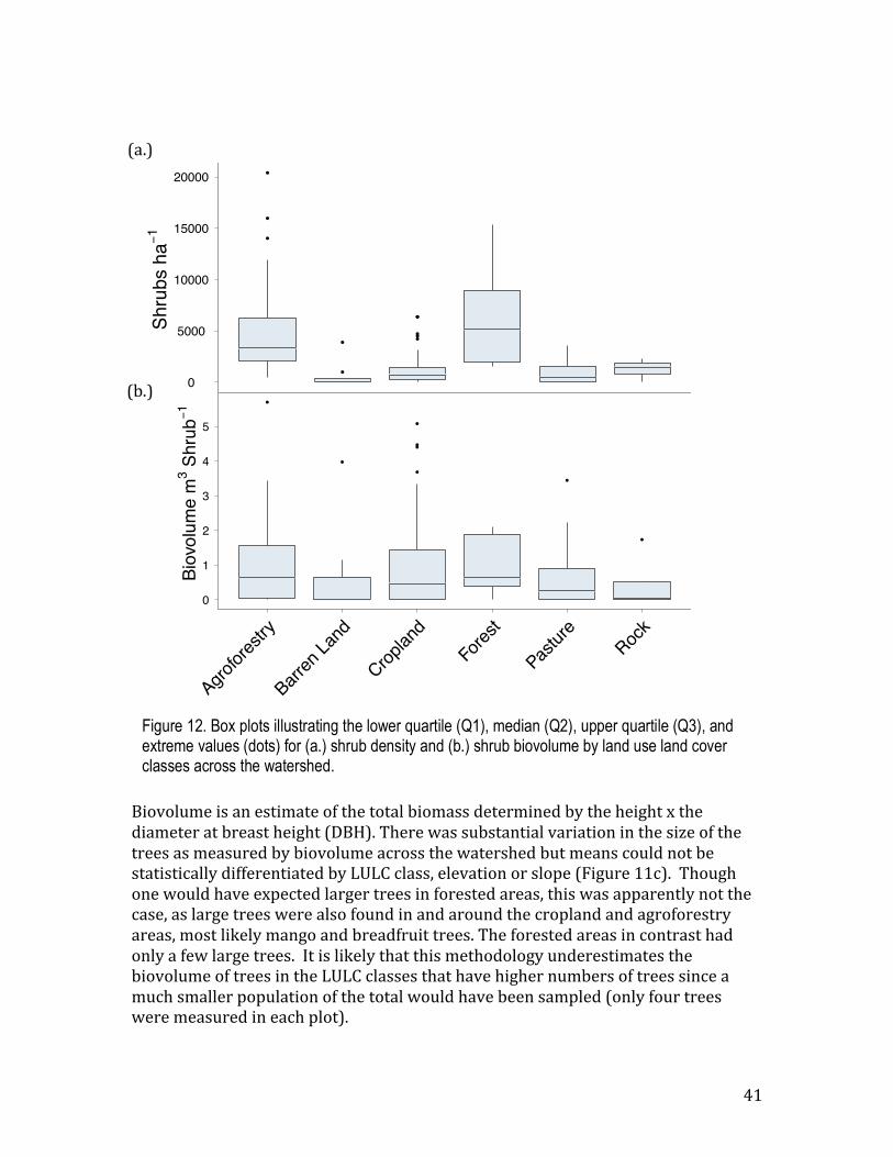
41
Biovolume is an estimate of the total biomass determined by the height x the diameter at breast height (DBH). There was substantial variation in the size of the trees as measured by biovolume across the watershed but means could not be statistically differentiated by LULC class, elevation or slope (Figure 11c). Though one would have expected larger trees in forested areas, this was apparently not the case, as large trees were also found in and around the cropland and agroforestry areas, most likely mango and breadfruit trees. The forested areas in contrast had only a few large trees. It is likely that this methodology underestimates the biovolume of trees in the LULC classes that have higher numbers of trees since a much smaller population of the total would have been sampled (only four trees were measured in each plot).
Shru
bs h
a!1
0
5000
10000
15000
20000
!
!
!
!
!
!
!
!
!!
Agrofor
estry
Barren
Land
Croplan
dFo
rest
Pastur
eRoc
k
Biov
olum
e m
3 Shr
ub!1
0
1
2
3
4
5
!
!
!
!
!
!
!
!
Agrofor
estry
Barren
Land
Croplan
dFo
rest
Pastur
eRoc
k
Figure 12. Box plots illustrating the lower quartile (Q1), median (Q2), upper quartile (Q3), and extreme values (dots) for (a.) shrub density and (b.) shrub biovolume by land use land cover classes across the watershed.
(a.)
(b.)
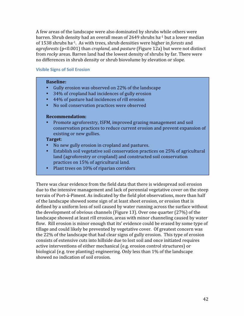
42
A few areas of the landscape were also dominated by shrubs while others were barren. Shrub density had an overall mean of 2649 shrubs ha-‐1 but a lower median of 1538 shrubs ha-‐1. As with trees, shrub densities were higher in forests and agroforests (p<0.001) than cropland, and pasture (Figure 12a) but were not distinct from rocky areas. Barren land had the lowest density of shrubs by far. There were no differences in shrub density or shrub biovolume by elevation or slope.
Visible Signs of Soil Erosion
There was clear evidence from the field data that there is widespread soil erosion due to the intensive management and lack of perennial vegetative cover on the steep terrain of Port-‐à-‐Piment. As indicated by the field plot observations, more than half of the landscape showed some sign of at least sheet erosion, or erosion that is defined by a uniform loss of soil caused by water running across the surface without the development of obvious channels (Figure 13). Over one quarter (27%) of the landscape showed at least rill erosion, areas with minor channeling caused by water flow. Rill erosion is minor enough that its’ evidence could be erased by some type of tillage and could likely be prevented by vegetative cover. Of greatest concern was the 22% of the landscape that had clear signs of gully erosion. This type of erosion consists of extensive cuts into hillside due to lost soil and once initiated requires active interventions of either mechanical (e.g. erosion control structures) or biological (e.g. tree planting) engineering. Only less than 1% of the landscape showed no indication of soil erosion.
Baseline: • Gully erosion was observed on 22% of the landscape • 34% of cropland had incidences of gully erosion • 44% of pasture had incidences of rill erosion • No soil conservation practices were observed Recommendation: • Promote agroforestry, ISFM, improved grazing management and soil
conservation practices to reduce current erosion and prevent expansion of existing or new gullies.
Target: • No new gully erosion in cropland and pastures. • Establish soil vegetative soil conservation practices on 25% of agricultural
land (agroforestry or cropland) and constructed soil conservation practices on 15% of agricultural land.
• Plant trees on 10% of riparian corridors
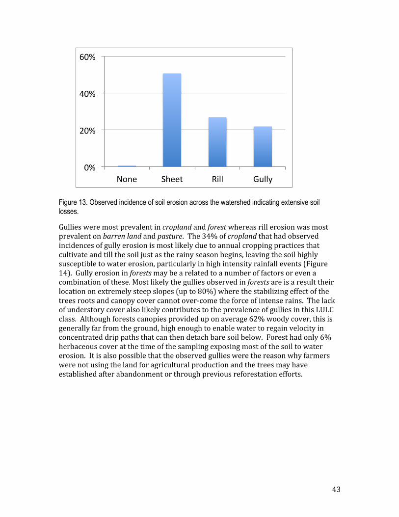
43
Figure 13. Observed incidence of soil erosion across the watershed indicating extensive soil losses.
Gullies were most prevalent in cropland and forest whereas rill erosion was most prevalent on barren land and pasture. The 34% of cropland that had observed incidences of gully erosion is most likely due to annual cropping practices that cultivate and till the soil just as the rainy season begins, leaving the soil highly susceptible to water erosion, particularly in high intensity rainfall events (Figure 14). Gully erosion in forests may be a related to a number of factors or even a combination of these. Most likely the gullies observed in forests are is a result their location on extremely steep slopes (up to 80%) where the stabilizing effect of the trees roots and canopy cover cannot over-‐come the force of intense rains. The lack of understory cover also likely contributes to the prevalence of gullies in this LULC class. Although forests canopies provided up on average 62% woody cover, this is generally far from the ground, high enough to enable water to regain velocity in concentrated drip paths that can then detach bare soil below. Forest had only 6% herbaceous cover at the time of the sampling exposing most of the soil to water erosion. It is also possible that the observed gullies were the reason why farmers were not using the land for agricultural production and the trees may have established after abandonment or through previous reforestation efforts.
!"#
$!"#
%!"#
&!"#
'()*# +,**-# ./00# 12003#

44
Figure 14. Percent distribution for the incidence of field observed soil erosion for each LULC class.
Although gully erosion was most prominent on steep slopes, there were substantial amounts observed on both level and moderate slopes (Figure 15). While these observations are qualitative and thus limited in their application, they provide an idea of the overall distribution of erosion severity and a benchmark indicator. In the section on Soil Erosion Risk we provide a map of the distribution of predicted soil erosion based on a soil erosion model. Despite the obvious signs of erosion we did not record any observations of soil conservation measures. Slope stabilization across the watershed is thus mainly contingent on the minimal tree or shrub cover, limited amount of pasture, and extensive annual cropping. Reducing soil erosion must be one of the highest priorities if watershed sustainability objectives are to be met. Unabated soil erosion not only results in the loss of the growth medium for plants it results in the loss of nutrients that the plants need for productivity. Furthermore soil particles and nutrients lost from the mountainsides end up in waterways at lower elevations impacting flooding regimes, water quality and fish stocks. Promoting a transition from annual cropping to agroforestry on steep or even moderate slopes, better planning and control of grazing to reduce impact and soil conservation practices could help reduce soil erosion substantially.
!"#
$%"#
%!"#
&%"#
'!!"#
()*+,+*-./*0#
12**-3#4235#
6*+78235#
9+*-./#
:2./;*-#
<+=>#
?+3-#
@A--/#
<B88#
C;880#
45
Figure 15. Observed incidence of soil erosion by slope class. The most severe erosion, gully, is most prevalent on steep slopes but is found throughout the watershed.
Soil Properties Physical and chemical soil properties varied greatly across the landscape and in some cases could be differentiated by LULC, slope, and/or elevation class. While it is challenging to determine what factors caused this variation, the large differences across the landscape indicate that there is a need for site-‐specific management recommendations and activities. Overall the major challenges presented by soil properties are related to topographic factors and ineffective nutrient cycling or replacement of nutrients lost from erosion or export by crop harvest.
Model Results Two sets of models were used for the analyses of soils properties, models that predict soil property values for each plot and then geospatial models that predict soil property values for locations found outside of the plots to produce contiguous maps of the watershed. The models used to calibrate near-‐ and mid-‐ infrared (NIR and MIR) spectra were robust for most of the properties analyzed (Table 6); 55% of the modeled soil properties had a coefficient of determination (R2) ≥ 0.90 and the confidence in these predictions is considered high. The R2 value for 34% of the model predictions was between 0.50-‐0.90 and considered to have medium confidence. Model R2 values less than 0.50 were considered to have low confidence and were only 10% of the total. These low confidence models included Mehlich-‐3 extractable phosphorus (P) and sulfur (S) and sand content The coefficient of
!"#
$!"#
%!"#
&!"#
'!"#
(!!"#
)*+
,#
-.,,/#
0122#
34225#
)*+
,#
-.,,/#
0122#
34225#
)*+
,#
-.,,/#
0122#
34225#
6,7,2# 8*9,:;/,# -/,,<#
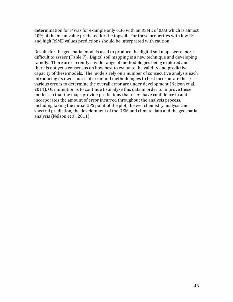
46
determination for P was for example only 0.36 with an RSME of 0.83 which is almost 40% of the mean value predicted for the topsoil. For these properties with low R2 and high RSME values predictions should be interpreted with caution. Results for the geospatial models used to produce the digital soil maps were more difficult to assess (Table 7). Digital soil mapping is a new technique and developing rapidly. There are currently a wide range of methodologies being explored and there is not yet a consensus on how best to evaluate the validity and predictive capacity of these models. The models rely on a number of consecutive analysis each introducing its own source of error and methodologies to best incorporate these various errors to determine the overall error are under development (Nelson et al. 2011). Our intention is to continue to analyze this data in order to improve these models so that the maps provide predictions that users have confidence in and incorporates the amount of error incurred throughout the analysis process, including taking the initial GPS point of the plot, the wet chemistry analysis and spectral prediction, the development of the DEM and climate data and the geospatial analysis (Nelson et al. 2011).
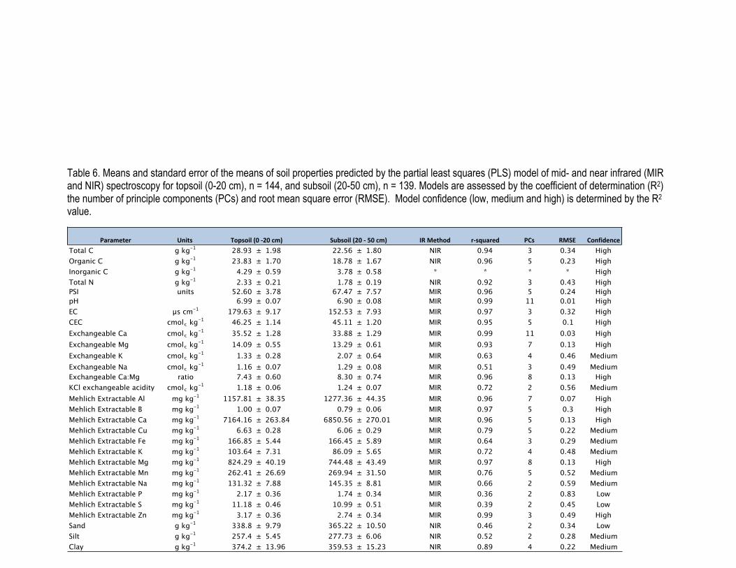
Table 6. Means and standard error of the means of soil properties predicted by the partial least squares (PLS) model of mid- and near infrared (MIR and NIR) spectroscopy for topsoil (0-20 cm), n = 144, and subsoil (20-50 cm), n = 139. Models are assessed by the coefficient of determination (R2) the number of principle components (PCs) and root mean square error (RMSE). Model confidence (low, medium and high) is determined by the R2
value.
!"#"$%&%# '()&* +,-.%&/01 -#2*34"#%1 !5* ,.67 50(8)1%(9%Total C g kg-1 28.93 ± 1.98 22.56 ± 1.80 NIR 0.94 3 0.34 HighOrganic C g kg-1 23.83 ± 1.70 18.78 ± 1.67 NIR 0.96 5 0.23 HighInorganic C g kg-1 4.29 ± 0.59 3.78 ± 0.58 * * * * HighTotal N g kg-1 2.33 ± 0.21 1.78 ± 0.19 NIR 0.92 3 0.43 HighPSI units 52.60 ± 3.78 67.47 ± 7.57 MIR 0.96 5 0.24 HighpH 6.99 ± 0.07 6.90 ± 0.08 MIR 0.99 11 0.01 HighEC μs cm-1 179.63 ± 9.17 152.53 ± 7.93 MIR 0.97 3 0.32 HighCEC cmolc kg-1 46.25 ± 1.14 45.11 ± 1.20 MIR 0.95 5 0.1 HighExchangeable Ca cmolc kg-1 35.52 ± 1.28 33.88 ± 1.29 MIR 0.99 11 0.03 HighExchangeable Mg cmolc kg-1 14.09 ± 0.55 13.29 ± 0.61 MIR 0.93 7 0.13 HighExchangeable K cmolc kg-1 1.33 ± 0.28 2.07 ± 0.64 MIR 0.63 4 0.46 MediumExchangeable Na cmolc kg-1 1.16 ± 0.07 1.29 ± 0.08 MIR 0.51 3 0.49 MediumExchangeable Ca:Mg ratio 7.43 ± 0.60 8.30 ± 0.74 MIR 0.96 8 0.13 HighKCl exchangeable acidity cmolc kg-1 1.18 ± 0.06 1.24 ± 0.07 MIR 0.72 2 0.56 MediumMehlich Extractable Al mg kg-1 1157.81 ± 38.35 1277.36 ± 44.35 MIR 0.96 7 0.07 HighMehlich Extractable B mg kg-1 1.00 ± 0.07 0.79 ± 0.06 MIR 0.97 5 0.3 HighMehlich Extractable Ca mg kg-1 7164.16 ± 263.84 6850.56 ± 270.01 MIR 0.96 5 0.13 HighMehlich Extractable Cu mg kg-1 6.63 ± 0.28 6.06 ± 0.29 MIR 0.79 5 0.22 MediumMehlich Extractable Fe mg kg-1 166.85 ± 5.44 166.45 ± 5.89 MIR 0.64 3 0.29 MediumMehlich Extractable K mg kg-1 103.64 ± 7.31 86.09 ± 5.65 MIR 0.72 4 0.48 MediumMehlich Extractable Mg mg kg-1 824.29 ± 40.19 744.48 ± 43.49 MIR 0.97 8 0.13 HighMehlich Extractable Mn mg kg-1 262.41 ± 26.69 269.94 ± 31.50 MIR 0.76 5 0.52 MediumMehlich Extractable Na mg kg-1 131.32 ± 7.88 145.35 ± 8.81 MIR 0.66 2 0.59 MediumMehlich Extractable P mg kg-1 2.17 ± 0.36 1.74 ± 0.34 MIR 0.36 2 0.83 LowMehlich Extractable S mg kg-1 11.18 ± 0.46 10.99 ± 0.51 MIR 0.39 2 0.45 LowMehlich Extractable Zn mg kg-1 3.17 ± 0.36 2.74 ± 0.34 MIR 0.99 3 0.49 HighSand g kg-1 338.8 ± 9.79 365.22 ± 10.50 NIR 0.46 2 0.34 LowSilt g kg-1 257.4 ± 5.45 277.73 ± 6.06 NIR 0.52 2 0.28 MediumClay g kg-1 374.2 ± 13.96 359.53 ± 15.23 NIR 0.89 4 0.22 Medium
:0;*0)<-=>-2?>-9$@ 64A*0)<-=?>-2-B>-9$@
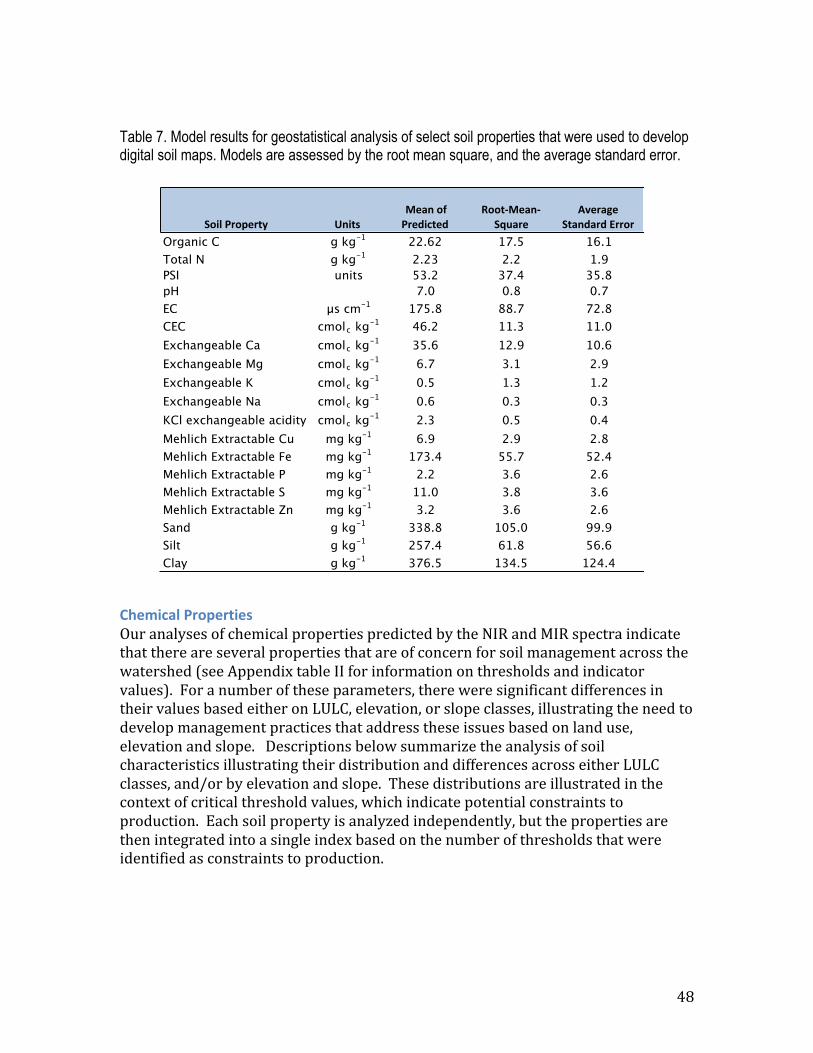
48
Table 7. Model results for geostatistical analysis of select soil properties that were used to develop digital soil maps. Models are assessed by the root mean square, and the average standard error.
Chemical Properties Our analyses of chemical properties predicted by the NIR and MIR spectra indicate that there are several properties that are of concern for soil management across the watershed (see Appendix table II for information on thresholds and indicator values). For a number of these parameters, there were significant differences in their values based either on LULC, elevation, or slope classes, illustrating the need to develop management practices that address these issues based on land use, elevation and slope. Descriptions below summarize the analysis of soil characteristics illustrating their distribution and differences across either LULC classes, and/or by elevation and slope. These distributions are illustrated in the context of critical threshold values, which indicate potential constraints to production. Each soil property is analyzed independently, but the properties are then integrated into a single index based on the number of thresholds that were identified as constraints to production.
!"#$%&'"()'*+ ,-#*./)0-%"1%&')2#3*)2
4""*5/)0-5!670')
89)'0:)%!*0-20'2%;''"'
Organic C g kg-1 22.62 17.5 16.1Total N g kg-1 2.23 2.2 1.9PSI units 53.2 37.4 35.8pH 7.0 0.8 0.7EC μs cm-1 175.8 88.7 72.8CEC cmolc kg-1 46.2 11.3 11.0Exchangeable Ca cmolc kg-1 35.6 12.9 10.6Exchangeable Mg cmolc kg-1 6.7 3.1 2.9Exchangeable K cmolc kg-1 0.5 1.3 1.2Exchangeable Na cmolc kg-1 0.6 0.3 0.3KCl exchangeable acidity cmolc kg-1 2.3 0.5 0.4Mehlich Extractable Cu mg kg-1 6.9 2.9 2.8Mehlich Extractable Fe mg kg-1 173.4 55.7 52.4Mehlich Extractable P mg kg-1 2.2 3.6 2.6Mehlich Extractable S mg kg-1 11.0 3.8 3.6Mehlich Extractable Zn mg kg-1 3.2 3.6 2.6Sand g kg-1 338.8 105.0 99.9Silt g kg-1 257.4 61.8 56.6Clay g kg-1 376.5 134.5 124.4
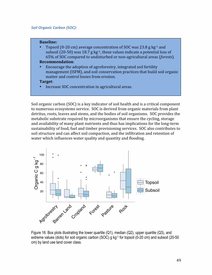
49
Soil Organic Carbon (SOC):
Soil organic carbon (SOC) is a key indicator of soil health and is a critical component to numerous ecosystems service. SOC is derived from organic materials from plant detritus, roots, leaves and stems, and the bodies of soil organisms. SOC provides the metabolic substrate required by microorganisms that ensure the cycling, storage and availability of many plant nutrients and thus has implications for the long-‐term sustainability of food, fuel and timber provisioning services. SOC also contributes to soil structure and can affect soil compaction, and the infiltration and retention of water which influences water quality and quantity and flooding.
Figure 16. Box plots illustrating the lower quartile (Q1), median (Q2), upper quartile (Q3), and extreme values (dots) for soil organic carbon (SOC) g kg-1 for topsoil (0-20 cm) and subsoil (20-50 cm) by land use land cover class.
Org
anic
C g
kg−
1
20
40
60
80
100 ●
●
●
●
●
●
●●
●
●
●
●
Agrofor
estry
Barren
Land
Croplan
dFo
rest
Pastur
eRoc
k
TopsoilSubsoil
Baseline: • Topsoil (0-‐20 cm) average concentration of SOC was 23.8 g kg-‐1 and
subsoil (20-‐50) was 18.7 g kg-‐1, these values indicate a potential loss of 65% of SOC compared to undisturbed or non-‐agricultural areas (forests).
Recommendation: • Encourage the adoption of agroforestry, integrated soil fertility
management (ISFM), and soil conservation practices that build soil organic matter and control losses from erosion.
Target: • Increase SOC concentration in agricultural areas.
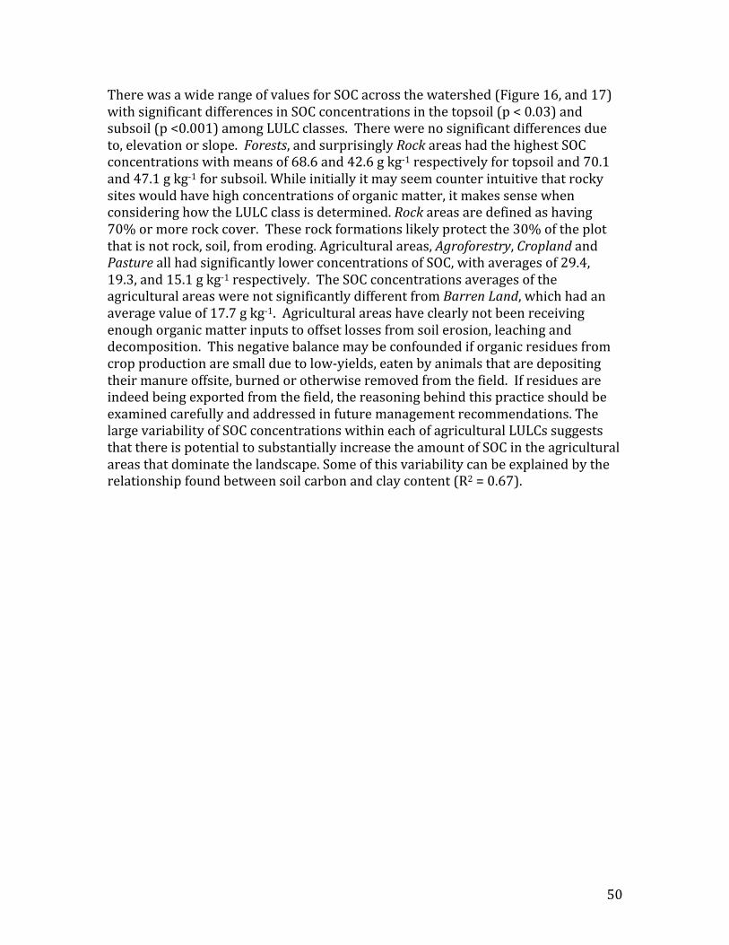
50
There was a wide range of values for SOC across the watershed (Figure 16, and 17) with significant differences in SOC concentrations in the topsoil (p < 0.03) and subsoil (p <0.001) among LULC classes. There were no significant differences due to, elevation or slope. Forests, and surprisingly Rock areas had the highest SOC concentrations with means of 68.6 and 42.6 g kg-‐1 respectively for topsoil and 70.1 and 47.1 g kg-‐1 for subsoil. While initially it may seem counter intuitive that rocky sites would have high concentrations of organic matter, it makes sense when considering how the LULC class is determined. Rock areas are defined as having 70% or more rock cover. These rock formations likely protect the 30% of the plot that is not rock, soil, from eroding. Agricultural areas, Agroforestry, Cropland and Pasture all had significantly lower concentrations of SOC, with averages of 29.4, 19.3, and 15.1 g kg-‐1 respectively. The SOC concentrations averages of the agricultural areas were not significantly different from Barren Land, which had an average value of 17.7 g kg-‐1. Agricultural areas have clearly not been receiving enough organic matter inputs to offset losses from soil erosion, leaching and decomposition. This negative balance may be confounded if organic residues from crop production are small due to low-‐yields, eaten by animals that are depositing their manure offsite, burned or otherwise removed from the field. If residues are indeed being exported from the field, the reasoning behind this practice should be examined carefully and addressed in future management recommendations. The large variability of SOC concentrations within each of agricultural LULCs suggests that there is potential to substantially increase the amount of SOC in the agricultural areas that dominate the landscape. Some of this variability can be explained by the relationship found between soil carbon and clay content (R2 = 0.67).
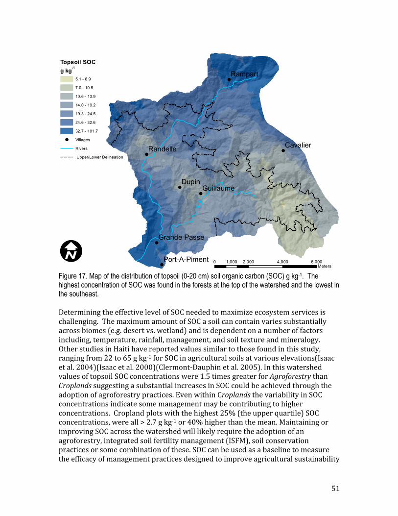
51
Figure 17. Map of the distribution of topsoil (0-20 cm) soil organic carbon (SOC) g kg-1. The highest concentration of SOC was found in the forests at the top of the watershed and the lowest in the southeast.
Determining the effective level of SOC needed to maximize ecosystem services is challenging. The maximum amount of SOC a soil can contain varies substantially across biomes (e.g. desert vs. wetland) and is dependent on a number of factors including, temperature, rainfall, management, and soil texture and mineralogy. Other studies in Haiti have reported values similar to those found in this study, ranging from 22 to 65 g kg-‐1 for SOC in agricultural soils at various elevations(Isaac et al. 2004)(Isaac et al. 2000)(Clermont-‐Dauphin et al. 2005). In this watershed values of topsoil SOC concentrations were 1.5 times greater for Agroforestry than Croplands suggesting a substantial increases in SOC could be achieved through the adoption of agroforestry practices. Even within Croplands the variability in SOC concentrations indicate some management may be contributing to higher concentrations. Cropland plots with the highest 25% (the upper quartile) SOC concentrations, were all > 2.7 g kg-‐1 or 40% higher than the mean. Maintaining or improving SOC across the watershed will likely require the adoption of an agroforestry, integrated soil fertility management (ISFM), soil conservation practices or some combination of these. SOC can be used as a baseline to measure the efficacy of management practices designed to improve agricultural sustainability
!
!
!
!
!
!
!
Dupin
Rampart
CavalierRandelle
Guillaume
Grande Passe
Port-A-Piment 0 2,000 4,000 6,0001,000Meters
I
Topsoil SOC
g kg-1
5.1 - 6.9
7.0 - 10.5
10.6 - 13.9
14.0 - 19.2
19.3 - 24.5
24.6 - 32.6
32.7 - 101.7
! Villages
Rivers
Upper/Lower Delineation
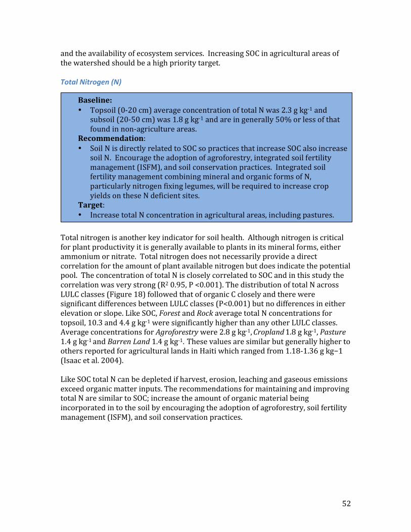
52
and the availability of ecosystem services. Increasing SOC in agricultural areas of the watershed should be a high priority target.
Total Nitrogen (N)
Total nitrogen is another key indicator for soil health. Although nitrogen is critical for plant productivity it is generally available to plants in its mineral forms, either ammonium or nitrate. Total nitrogen does not necessarily provide a direct correlation for the amount of plant available nitrogen but does indicate the potential pool. The concentration of total N is closely correlated to SOC and in this study the correlation was very strong (R2 0.95, P <0.001). The distribution of total N across LULC classes (Figure 18) followed that of organic C closely and there were significant differences between LULC classes (P<0.001) but no differences in either elevation or slope. Like SOC, Forest and Rock average total N concentrations for topsoil, 10.3 and 4.4 g kg-‐1 were significantly higher than any other LULC classes. Average concentrations for Agroforestry were 2.8 g kg-‐1, Cropland 1.8 g kg-‐1, Pasture 1.4 g kg-‐1 and Barren Land 1.4 g kg-‐1. These values are similar but generally higher to others reported for agricultural lands in Haiti which ranged from 1.18-‐1.36 g kg−1 (Isaac et al. 2004). Like SOC total N can be depleted if harvest, erosion, leaching and gaseous emissions exceed organic matter inputs. The recommendations for maintaining and improving total N are similar to SOC; increase the amount of organic material being incorporated in to the soil by encouraging the adoption of agroforestry, soil fertility management (ISFM), and soil conservation practices.
Baseline: • Topsoil (0-‐20 cm) average concentration of total N was 2.3 g kg-‐1 and
subsoil (20-‐50 cm) was 1.8 g kg-‐1 and are in generally 50% or less of that found in non-‐agriculture areas.
Recommendation: • Soil N is directly related to SOC so practices that increase SOC also increase
soil N. Encourage the adoption of agroforestry, integrated soil fertility management (ISFM), and soil conservation practices. Integrated soil fertility management combining mineral and organic forms of N, particularly nitrogen fixing legumes, will be required to increase crop yields on these N deficient sites.
Target: • Increase total N concentration in agricultural areas, including pastures.
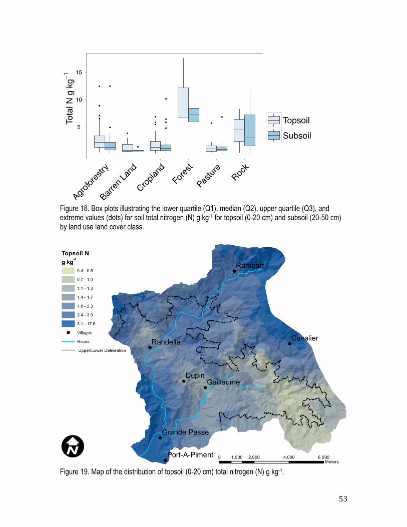
53
Figure 18. Box plots illustrating the lower quartile (Q1), median (Q2), upper quartile (Q3), and extreme values (dots) for soil total nitrogen (N) g kg-1 for topsoil (0-20 cm) and subsoil (20-50 cm) by land use land cover class.
Figure 19. Map of the distribution of topsoil (0-20 cm) total nitrogen (N) g kg-1.
Tota
l N g
kg−
1
5
10
15
●
●
●
●
●
●
●
●
●
●●
●
●
●
●
●
●
Agrofor
estry
Barren
Land
Croplan
dFo
rest
Pastur
eRoc
k
TopsoilSubsoil
!
!
!
!
!
!
!
Dupin
Rampart
CavalierRandelle
Guillaume
Grande Passe
Port-A-Piment 0 2,000 4,000 6,0001,000Meters
I
Topsoil N g kg-1
0.4 - 0.6
0.7 - 1.0
1.1 - 1.3
1.4 - 1.7
1.8 - 2.3
2.4 - 3.0
3.1 - 17.6
! Villages
Rivers
Upper/Lower Delineation
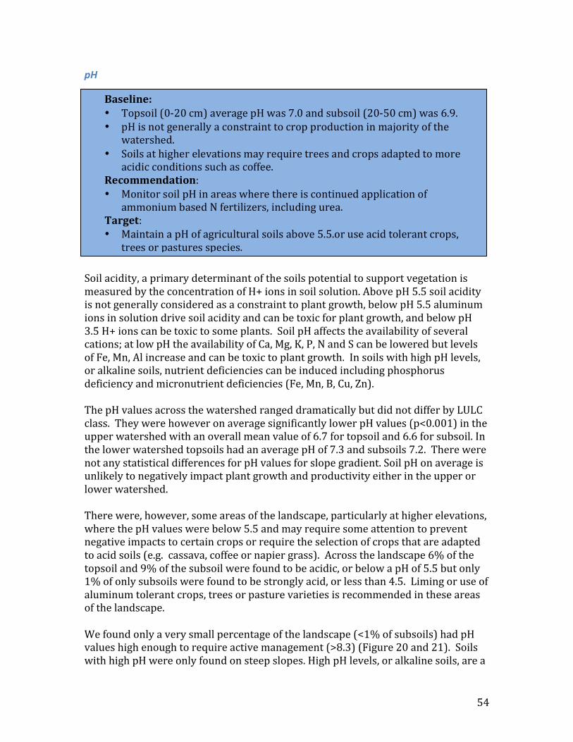
54
pH
Soil acidity, a primary determinant of the soils potential to support vegetation is measured by the concentration of H+ ions in soil solution. Above pH 5.5 soil acidity is not generally considered as a constraint to plant growth, below pH 5.5 aluminum ions in solution drive soil acidity and can be toxic for plant growth, and below pH 3.5 H+ ions can be toxic to some plants. Soil pH affects the availability of several cations; at low pH the availability of Ca, Mg, K, P, N and S can be lowered but levels of Fe, Mn, Al increase and can be toxic to plant growth. In soils with high pH levels, or alkaline soils, nutrient deficiencies can be induced including phosphorus deficiency and micronutrient deficiencies (Fe, Mn, B, Cu, Zn). The pH values across the watershed ranged dramatically but did not differ by LULC class. They were however on average significantly lower pH values (p<0.001) in the upper watershed with an overall mean value of 6.7 for topsoil and 6.6 for subsoil. In the lower watershed topsoils had an average pH of 7.3 and subsoils 7.2. There were not any statistical differences for pH values for slope gradient. Soil pH on average is unlikely to negatively impact plant growth and productivity either in the upper or lower watershed. There were, however, some areas of the landscape, particularly at higher elevations, where the pH values were below 5.5 and may require some attention to prevent negative impacts to certain crops or require the selection of crops that are adapted to acid soils (e.g. cassava, coffee or napier grass). Across the landscape 6% of the topsoil and 9% of the subsoil were found to be acidic, or below a pH of 5.5 but only 1% of only subsoils were found to be strongly acid, or less than 4.5. Liming or use of aluminum tolerant crops, trees or pasture varieties is recommended in these areas of the landscape. We found only a very small percentage of the landscape (<1% of subsoils) had pH values high enough to require active management (>8.3) (Figure 20 and 21). Soils with high pH were only found on steep slopes. High pH levels, or alkaline soils, are a
Baseline: • Topsoil (0-‐20 cm) average pH was 7.0 and subsoil (20-‐50 cm) was 6.9. • pH is not generally a constraint to crop production in majority of the
watershed. • Soils at higher elevations may require trees and crops adapted to more
acidic conditions such as coffee. Recommendation: • Monitor soil pH in areas where there is continued application of
ammonium based N fertilizers, including urea. Target: • Maintain a pH of agricultural soils above 5.5.or use acid tolerant crops,
trees or pastures species.
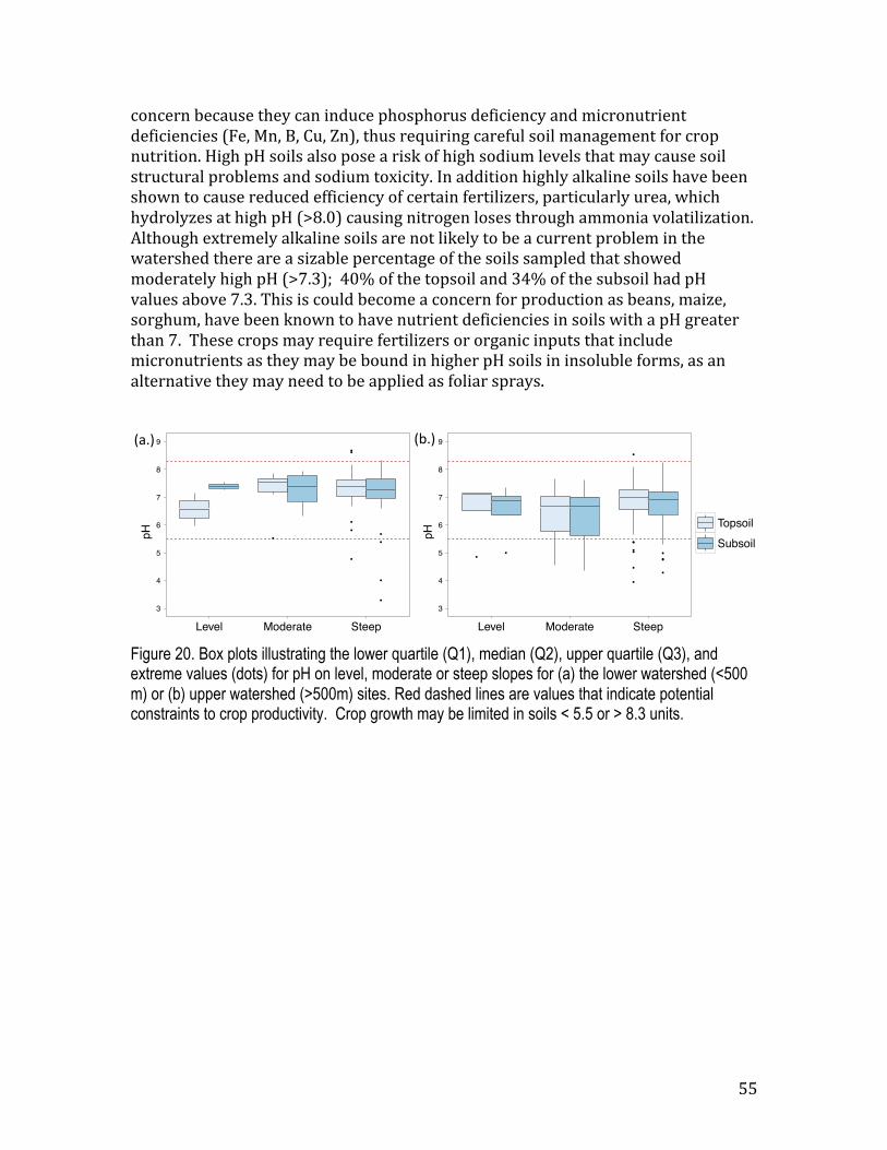
55
concern because they can induce phosphorus deficiency and micronutrient deficiencies (Fe, Mn, B, Cu, Zn), thus requiring careful soil management for crop nutrition. High pH soils also pose a risk of high sodium levels that may cause soil structural problems and sodium toxicity. In addition highly alkaline soils have been shown to cause reduced efficiency of certain fertilizers, particularly urea, which hydrolyzes at high pH (>8.0) causing nitrogen loses through ammonia volatilization. Although extremely alkaline soils are not likely to be a current problem in the watershed there are a sizable percentage of the soils sampled that showed moderately high pH (>7.3); 40% of the topsoil and 34% of the subsoil had pH values above 7.3. This is could become a concern for production as beans, maize, sorghum, have been known to have nutrient deficiencies in soils with a pH greater than 7. These crops may require fertilizers or organic inputs that include micronutrients as they may be bound in higher pH soils in insoluble forms, as an alternative they may need to be applied as foliar sprays.
Figure 20. Box plots illustrating the lower quartile (Q1), median (Q2), upper quartile (Q3), and extreme values (dots) for pH on level, moderate or steep slopes for (a) the lower watershed (<500 m) or (b) upper watershed (>500m) sites. Red dashed lines are values that indicate potential constraints to crop productivity. Crop growth may be limited in soils < 5.5 or > 8.3 units.
!"#$% !&#$%
pH
3
4
5
6
7
8
9
!
!
!
!!
!
!
!
!
!
Level Moderate Steep
TopsoilSubsoilpH
3
4
5
6
7
8
9
!
!
!
!!
!
!
!
!
!
!
!!
Level Moderate Steep
TopsoilSubsoil
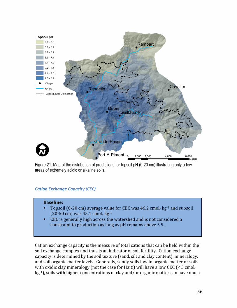
56
Figure 21. Map of the distribution of predictions for topsoil pH (0-20 cm) illustrating only a few areas of extremely acidic or alkaline soils.
Cation Exchange Capacity (CEC)
Cation exchange capacity is the measure of total cations that can be held within the soil exchange complex and thus is an indicator of soil fertility. Cation exchange capacity is determined by the soil texture (sand, silt and clay content), mineralogy, and soil organic matter levels. Generally, sandy soils low in organic matter or soils with oxidic clay mineralogy (not the case for Haiti) will have a low CEC (< 3 cmolc kg-‐1), soils with higher concentrations of clay and/or organic matter can have much
!
!
!
!
!
!
!
Dupin
Rampart
CavalierRandelle
Guillaume
Grande Passe
Port-A-Piment 0 2,000 4,000 6,0001,000Meters
I
Topsoil pH
3.9 - 5.8
5.8 - 6.7
6.7 - 6.9
6.9 - 7.1
7.1 - 7.2
7.2 - 7.4
7.4 - 7.5
7.5 - 8.7
! Villages
Rivers
Upper/Lower Delineation
Baseline: • Topsoil (0-‐20 cm) average value for CEC was 46.2 cmolc kg-‐1 and subsoil
(20-‐50 cm) was 45.1 cmolc kg-‐1 • CEC is generally high across the watershed and is not considered a
constraint to production as long as pH remains above 5.5.
57
higher CEC (> 20 cmolc kg-‐1). Soils with a high percentage of basic cations held on the exchange sites (% base saturation) are generally of high fertility compared to soils with a low base saturation or high exchangeable aluminum saturation. Soils with low cation exchange capacity do not hold on to nutrients so may be at risk of nutrient leaching. Loss of nutrients can reduce plant productivity and lead to negative environmental consequences. There were no significant differences in CEC among LULC classes. There were significant differences in CEC for both elevation and slope for topsoil but only for elevation for the subsoil. Mean CEC in the upper watershed was 40.0 cmolc kg-‐1 and in the lower watershed and 54.7 cmolc kg-‐1 (Figure 22). The lowest values for CEC were predicted to be at the very top of the watershed (Figure 23). Higher CEC downslope is not unusual as clay particles and soil organic matter wash and accumulate downhill. Mean CEC values here were higher than highest values reported in a nearby study which ranged from 12.1 to 33.3 cmolc kg-‐1 (Clermont-‐Dauphin et al. 2005); but this may be due to differences in methodologies.
Figure 22. Box plots illustrating the lower quartile (Q1), median (Q2), upper quartile (Q3), and extreme values (dots) for cation exchange capacity (CEC) cmolc kg-1 on level, moderate or steep slopes for (a) low elevation (<500 m) or (b) high elevation (>500m) sites. All of the values are considered high and not a constraint for production.
!"#$% !&#$%
Cat
ion
Exch
ange
Cap
acity
cm
olc k
g!1
20
30
40
50
60
70
80!
!
Level Moderate Steep
TopsoilSubsoil
Cat
ion
Exch
ange
Cap
acity
cm
olc k
g!1
20
30
40
50
60
70
80
Level Moderate Steep
TopsoilSubsoil
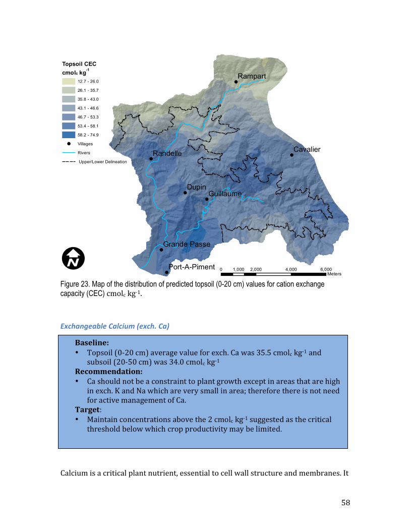
58
Figure 23. Map of the distribution of predicted topsoil (0-20 cm) values for cation exchange capacity (CEC) cmolc kg-‐1.
Exchangeable Calcium (exch. Ca)
Calcium is a critical plant nutrient, essential to cell wall structure and membranes. It
!
!
!
!
!
!
!
Dupin
Rampart
CavalierRandelle
Guillaume
Grande Passe
Port-A-Piment 0 2,000 4,000 6,0001,000Meters
I
Topsoil CECcmolc kg-1
12.7 - 26.0
26.1 - 35.7
35.8 - 43.0
43.1 - 46.6
46.7 - 53.3
53.4 - 58.1
58.2 - 74.9
! Villages
Rivers
Upper/Lower Delineation
Baseline: • Topsoil (0-‐20 cm) average value for exch. Ca was 35.5 cmolc kg-‐1 and
subsoil (20-‐50 cm) was 34.0 cmolc kg-‐1 Recommendation: • Ca should not be a constraint to plant growth except in areas that are high
in exch. K and Na which are very small in area; therefore there is not need for active management of Ca.
Target: • Maintain concentrations above the 2 cmolc kg-‐1 suggested as the critical
threshold below which crop productivity may be limited.
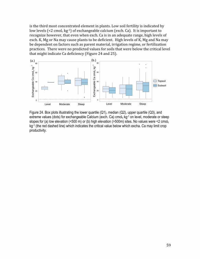
59
is the third most concentrated element in plants. Low soil fertility is indicated by low levels (<2 cmolc kg-‐1) of exchangeable calcium (exch. Ca). It is important to recognize however, that even when exch. Ca is in an adequate range, high levels of exch. K, Mg or Na may cause plants to be deficient. High levels of K, Mg and Na may be dependent on factors such as parent material, irrigation regime, or fertilization practices. There were no predicted values for soils that were below the critical level that might indicate Ca deficiency (Figure 24 and 25).
Figure 24. Box plots illustrating the lower quartile (Q1), median (Q2), upper quartile (Q3), and extreme values (dots) for exchangeable Calcium (exch. Ca) cmolc kg-1 on level, moderate or steep slopes for (a) low elevation (<500 m) or (b) high elevation (>500m) sites. No values were <2 cmolc kg-1 (the red dashed line) which indicates the critical value below which excha. Ca may limit crop productivity.
!"#$% !&#$%
Exch
ange
able
Ca
cmol
c kg!
1
0
20
40
60
80
!
!
!!
Level Moderate Steep
TopsoilSubsoil
Exch
ange
able
Ca
cmol
c kg!
1
0
20
40
60
80!
!
!
Level Moderate Steep
TopsoilSubsoil
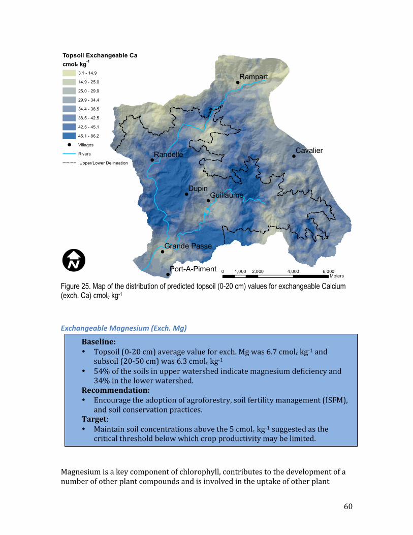
60
Figure 25. Map of the distribution of predicted topsoil (0-20 cm) values for exchangeable Calcium (exch. Ca) cmolc kg-1
Exchangeable Magnesium (Exch. Mg)
Magnesium is a key component of chlorophyll, contributes to the development of a number of other plant compounds and is involved in the uptake of other plant
!
!
!
!
!
!
!
Dupin
Rampart
CavalierRandelle
Guillaume
Grande Passe
Port-A-Piment 0 2,000 4,000 6,0001,000Meters
I
Topsoil Exchangeable Cacmolc kg-1
3.1 - 14.9
14.9 - 25.0
25.0 - 29.9
29.9 - 34.4
34.4 - 38.5
38.5 - 42.5
42.5 - 45.1
45.1 - 86.2
! Villages
Rivers
Upper/Lower Delineation
Baseline: • Topsoil (0-‐20 cm) average value for exch. Mg was 6.7 cmolc kg-‐1 and
subsoil (20-‐50 cm) was 6.3 cmolc kg-‐1 • 54% of the soils in upper watershed indicate magnesium deficiency and
34% in the lower watershed. Recommendation: • Encourage the adoption of agroforestry, soil fertility management (ISFM),
and soil conservation practices. Target: • Maintain soil concentrations above the 5 cmolc kg-‐1 suggested as the
critical threshold below which crop productivity may be limited.
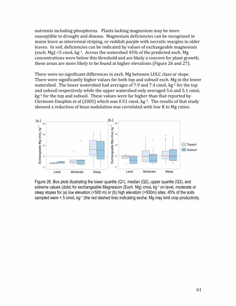
61
nutrients including phosphorus. Plants lacking magnesium may be more susceptible to drought and disease. Magnesium deficiencies can be recognized in maize leave as interveinal striping, or reddish purple with necrotic margins in older leaves. In soil, deficiencies can be indicated by values of exchangeable magnesium (exch. Mg) <5 cmolc kg-‐1. Across the watershed 45% of the predicted exch. Mg concentrations were below this threshold and are likely a concern for plant growth; these areas are more likely to be found at higher elevations (Figure 26 and 27). There were no significant differences in exch. Mg between LULC class or slope. There were significantly higher values for both top and subsoil exch. Mg in the lower watershed. The lower watershed had averages of 7.9 and 7.4 cmolc kg-‐1 for the top and subsoil respectively while the upper watershed only averaged 5.6 and 5.1 cmolc kg-‐1 for the top and subsoil. These values were far higher than that reported by Clermont-‐Dauphin et al (2005) which was 0.51 cmolc kg-‐1. The results of that study showed a reduction of bean nodulation was correlated with low K to Mg ratios.
Figure 26. Box plots illustrating the lower quartile (Q1), median (Q2), upper quartile (Q3), and extreme values (dots) for exchangeable Magnesium (Exch. Mg) cmolc kg-1 on level, moderate or steep slopes for (a) low elevation (<500 m) or (b) high elevation (>500m) sites. 45% of the soils sampled were < 5 cmolc kg-1 (the red dashed line) indicating excha. Mg may limit crop productivity.
!"#$% !&#$%
Exch
ange
able
Mg
cmol
c kg!
1
0
5
10
15
20
!
!
Level Moderate Steep
TopsoilSubsoil
Exch
ange
able
Mg
cmol
c kg!
1
0
5
10
15
20
!
!!!
!
Level Moderate Steep
TopsoilSubsoil
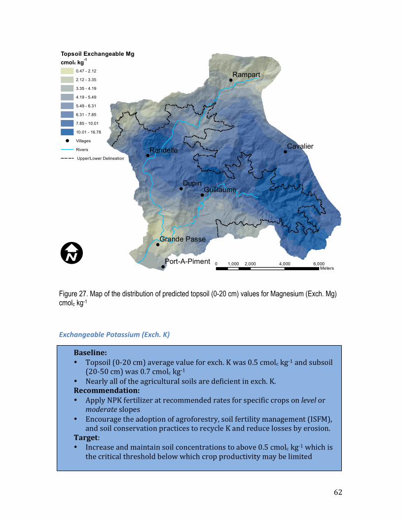
62
Figure 27. Map of the distribution of predicted topsoil (0-20 cm) values for Magnesium (Exch. Mg) cmolc kg-1
Exchangeable Potassium (Exch. K)
!
!
!
!
!
!
!
Dupin
Rampart
CavalierRandelle
Guillaume
Grande Passe
Port-A-Piment 0 2,000 4,000 6,0001,000Meters
I
Topsoil Exchangeable Mgcmolc kg-1
0.47 - 2.12
2.12 - 3.35
3.35 - 4.19
4.19 - 5.49
5.49 - 6.31
6.31 - 7.85
7.85 - 10.01
10.01 - 16.78
! Villages
Rivers
Upper/Lower Delineation
Baseline: • Topsoil (0-‐20 cm) average value for exch. K was 0.5 cmolc kg-‐1 and subsoil
(20-‐50 cm) was 0.7 cmolc kg-‐1 • Nearly all of the agricultural soils are deficient in exch. K. Recommendation: • Apply NPK fertilizer at recommended rates for specific crops on level or
moderate slopes • Encourage the adoption of agroforestry, soil fertility management (ISFM),
and soil conservation practices to recycle K and reduce losses by erosion. Target: • Increase and maintain soil concentrations to above 0.5 cmolc kg-‐1 which is
the critical threshold below which crop productivity may be limited
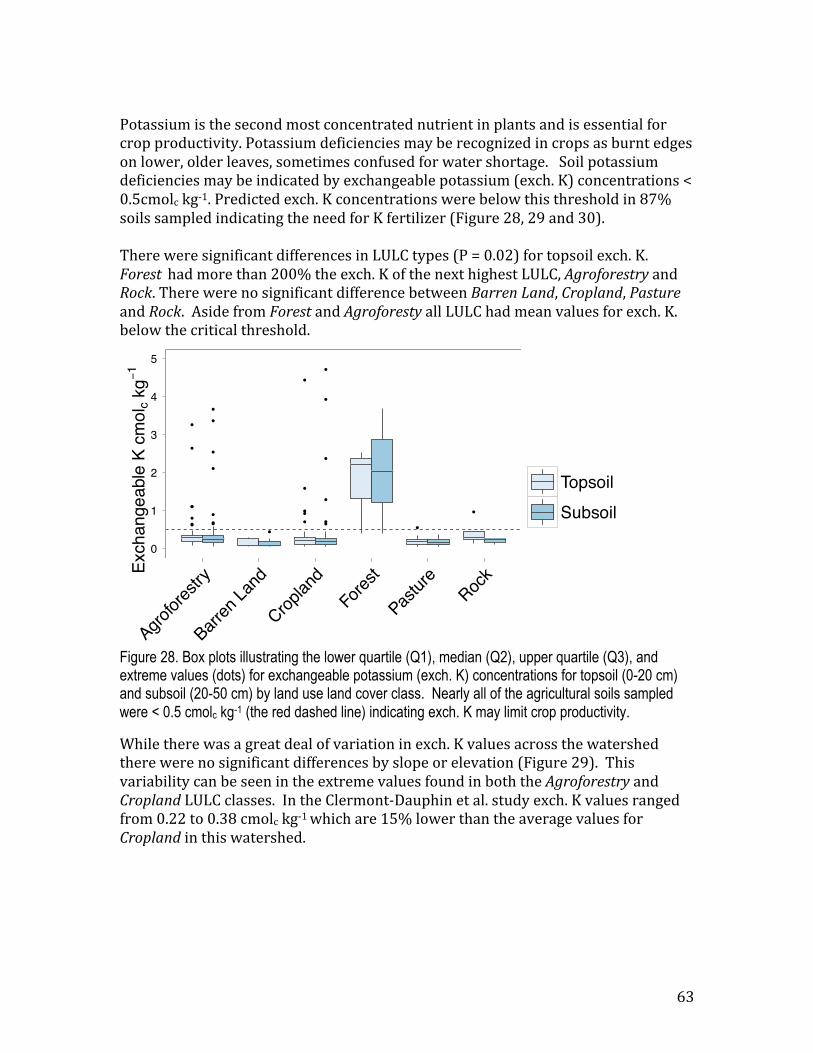
63
Potassium is the second most concentrated nutrient in plants and is essential for crop productivity. Potassium deficiencies may be recognized in crops as burnt edges on lower, older leaves, sometimes confused for water shortage. Soil potassium deficiencies may be indicated by exchangeable potassium (exch. K) concentrations < 0.5cmolc kg-‐1. Predicted exch. K concentrations were below this threshold in 87% soils sampled indicating the need for K fertilizer (Figure 28, 29 and 30). There were significant differences in LULC types (P = 0.02) for topsoil exch. K. Forest had more than 200% the exch. K of the next highest LULC, Agroforestry and Rock. There were no significant difference between Barren Land, Cropland, Pasture and Rock. Aside from Forest and Agroforesty all LULC had mean values for exch. K. below the critical threshold.
Figure 28. Box plots illustrating the lower quartile (Q1), median (Q2), upper quartile (Q3), and extreme values (dots) for exchangeable potassium (exch. K) concentrations for topsoil (0-20 cm) and subsoil (20-50 cm) by land use land cover class. Nearly all of the agricultural soils sampled were < 0.5 cmolc kg-1 (the red dashed line) indicating exch. K may limit crop productivity.
While there was a great deal of variation in exch. K values across the watershed there were no significant differences by slope or elevation (Figure 29). This variability can be seen in the extreme values found in both the Agroforestry and Cropland LULC classes. In the Clermont-‐Dauphin et al. study exch. K values ranged from 0.22 to 0.38 cmolc kg-‐1 which are 15% lower than the average values for Cropland in this watershed.
Exch
ange
able
K c
mol
c kg−
1
0
1
2
3
4
5
●
●
●
●
●●
●
●
●
●
●
●
●
●
●
●
●
●
●
●
●
●
●●
●
●
●
●
Agrofor
estry
Barren
Land
Croplan
dFo
rest
Pastur
eRoc
k
TopsoilSubsoil
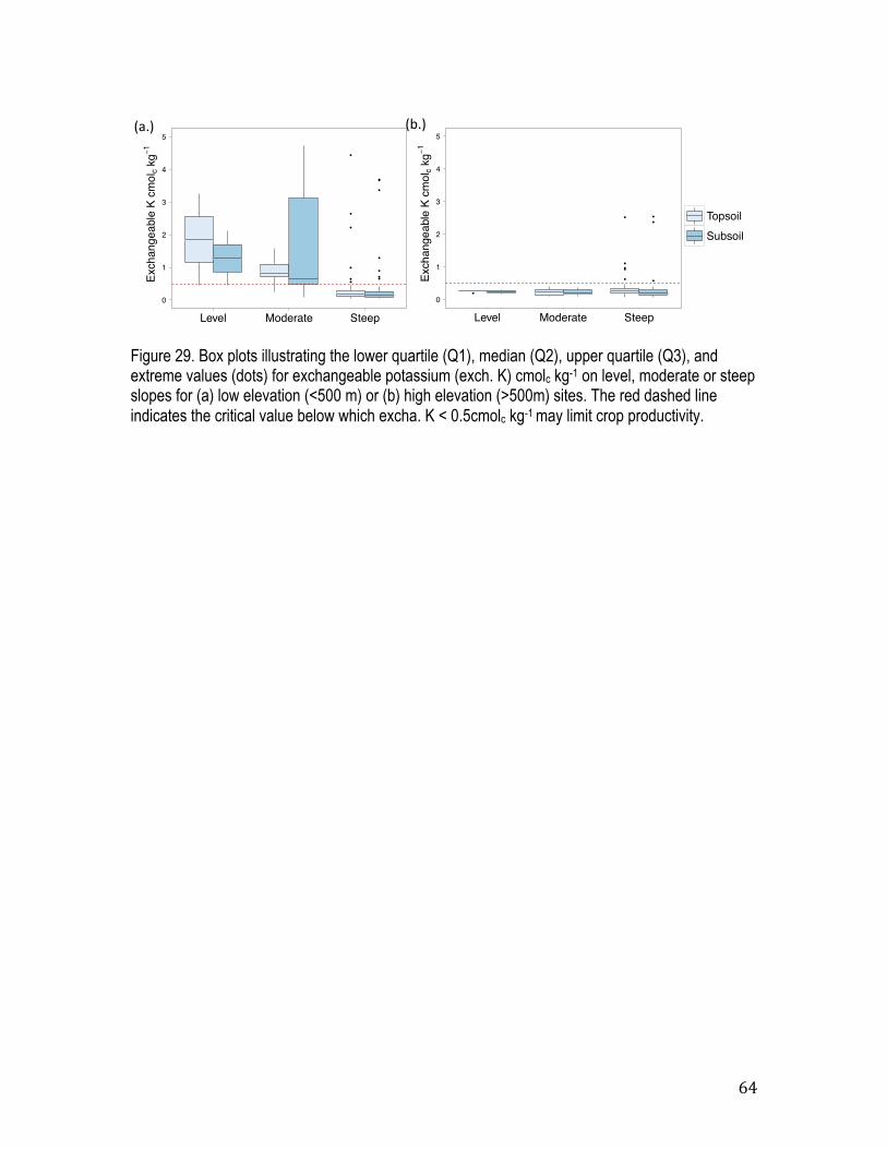
64
Figure 29. Box plots illustrating the lower quartile (Q1), median (Q2), upper quartile (Q3), and extreme values (dots) for exchangeable potassium (exch. K) cmolc kg-1 on level, moderate or steep slopes for (a) low elevation (<500 m) or (b) high elevation (>500m) sites. The red dashed line indicates the critical value below which excha. K < 0.5cmolc kg-1 may limit crop productivity.
!"#$% !&#$%
Exch
ange
able
K c
mol
c kg!
1
0
1
2
3
4
5
!
!
!
!!
!
!!
!
!
!
!
!
Level Moderate Steep
TopsoilSubsoil
Exch
ange
able
K c
mol
c kg!
1
0
1
2
3
4
5
!
!!
!
!
!
!
!
!
Level Moderate Steep
TopsoilSubsoil

65
Figure 30. Map of the distribution of (top) predicted topsoil (0-20 cm) values for exchangeable potassium (exch. K) cmolc kg-1 and (bottom) areas below the critical threshold that may indicate potential constraints fro crop production.
!
!
!
!
!
!
!
Dupin
Rampart
CavalierRandelle
Guillaume
Grande Passe
Port-A-Piment 0 2,000 4,000 6,0001,000Meters
I
Topsoil Exchangeable K Thresholdcmolc kg-1
<0.5
0.6 - 13.0
Upper/Lower Delineation
Rivers
! Villages
!
!
!
!
!
!
!
Dupin
Rampart
CavalierRandelle
Guillaume
Grande Passe
Port-A-Piment 0 2,000 4,000 6,0001,000Meters
I
Topsoil Exchangeable Kcmolc kg-1
0.05 - 0.09
0.09 - 0.13
0.13 - 0.19
0.19 - 0.22
0.22 - 0.26
0.26 - 0.29
0.29 - 0.35
0.35 - 13.0
! Villages
Rivers
Upper/Lower Delineation

66
Exchangeable Sodium (exch. Na)
Soil structure can be affected by high concentrations of exchangeable sodium (exch. Na). Erosion risk can increase, and infiltration rates can be reduced in soils with exch. Na concentrations >1 cmolc kg-‐1. Across the watershed 23% of the topsoils were predicted to have values above this critical level. There were no significant differences detected between LULC classes. There however were significant differences in elevation and in slope by elevation for both the topsoil (P<0.01) and subsoil (P=0.01) (Figure 31 and 32). Topsoil on Steep slopes had >100% more Na than either Moderate or Level slope while subsoil had >60%. Values for exch. Na were 100% and 82% higher in the lower watershed for topsoil and subsoil respectively.
31. Box plots illustrating the lower quartile (Q1), median (Q2), upper quartile (Q3), and extreme values (dots) for exchangeable Na cmolc kg-1 on level, moderate or steep slopes for (a) low elevation (<500 m) or (b) high elevation (>500m) sites. The red dashed line indicates the critical value above which excha. Na may negatively impact soil structure (> 1 cmolc kg-1).
!"#$% !&#$%
Exch
ange
able
Na
cmol
c kg!
1
0.0
0.5
1.0
1.5
2.0
2.5
!
Level Moderate Steep
TopsoilSubsoil
Exch
ange
able
Na
cmol
c kg!
1
0.0
0.5
1.0
1.5
2.0
2.5
!
!
!
!!
!
!
!
!
!!
!
!
!
!
!!
!
!!!
Level Moderate Steep
TopsoilSubsoil
Baseline: • Topsoil (0-‐20 cm) average value for exch. Na was 0.5 cmolc kg-‐1 and
subsoil (20-‐50 cm) was 0.6 cmolc kg-‐1 • 10% of the soils in upper watershed have high levels of exch. Na, and 35%
in the lower watershed. Target: 1.0 cmolc kg-‐1 is the critical threshold above which crop productivity may be limited
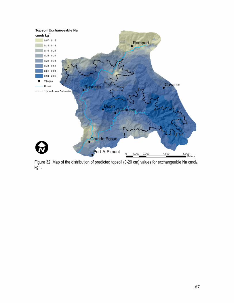
67
Figure 32. Map of the distribution of predicted topsoil (0-20 cm) values for exchangeable Na cmolc kg-1.
!
!
!
!
!
!
!
Dupin
Rampart
CavalierRandelle
Guillaume
Grande Passe
Port-A-Piment 0 2,000 4,000 6,0001,000Meters
I
Topsoil Exchangeable Nacmolc kg-1
0.07 - 0.15
0.15 - 0.19
0.19 - 0.24
0.24 - 0.29
0.29 - 0.38
0.38 - 0.61
0.61 - 0.94
0.94 - 2.00
! Villages
Rivers
Upper/Lower Delineation
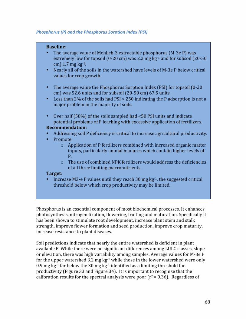
68
Phosphorus (P) and the Phosphorus Sorption Index (PSI)
Phosphorus is an essential component of most biochemical processes. It enhances photosynthesis, nitrogen fixation, flowering, fruiting and maturation. Specifically it has been shown to stimulate root development, increase plant stem and stalk strength, improve flower formation and seed production, improve crop maturity, increase resistance to plant diseases. Soil predictions indicate that nearly the entire watershed is deficient in plant available P. While there were no significant differences among LULC classes, slope or elevation, there was high variability among samples. Average values for M-‐3e P for the upper watershed 3.2 mg kg-‐1 while those in the lower watershed were only 0.9 mg kg-‐1 far below the 30 mg kg-‐1 identified as a limiting threshold for productivity (Figure 33 and Figure 34). It is important to recognize that the calibration results for the spectral analysis were poor (r2 = 0.36). Regardless of
Baseline: • The average value of Mehlich-‐3 extractable phosphorus (M-‐3e P) was
extremely low for topsoil (0-‐20 cm) was 2.2 mg kg-‐1 and for subsoil (20-‐50 cm) 1.7 mg kg-‐1.
• Nearly all of the soils in the watershed have levels of M-‐3e P below critical values for crop growth.
• The average value the Phosphorus Sorption Index (PSI) for topsoil (0-‐20 cm) was 52.6 units and for subsoil (20-‐50 cm) 67.5 units.
• Less than 2% of the soils had PSI > 250 indicating the P adsorption is not a major problem in the majority of soils.
• Over half (58%) of the soils sampled had <50 PSI units and indicate potential problems of P leaching with excessive application of fertilizers.
Recommendation: • Addressing soil P deficiency is critical to increase agricultural productivity. • Promote:
o Application of P fertilizers combined with increased organic matter inputs, particularly animal manures which contain higher levels of P.
o The use of combined NPK fertilizers would address the deficiencies of all three limiting macronutrients.
Target: • Increase M3-‐e P values until they reach 30 mg kg-‐1, the suggested critical
threshold below which crop productivity may be limited.
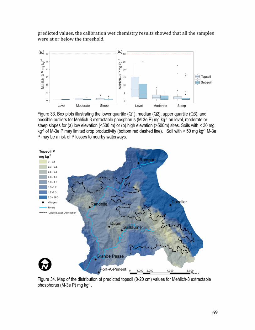
69
predicted values, the calibration wet chemistry results showed that all the samples were at or below the threshold.
Figure 33. Box plots illustrating the lower quartile (Q1), median (Q2), upper quartile (Q3), and possible outliers for Mehlich-3 extractable phosphorus (M-3e P) mg kg-1 on level, moderate or steep slopes for (a) low elevation (<500 m) or (b) high elevation (>500m) sites. Soils with < 30 mg kg-1 of M-3e P may limited crop productivity (bottom red dashed line). Soil with > 50 mg kg-1 M-3e P may be a risk of P losses to nearby waterways.
Figure 34. Map of the distribution of predicted topsoil (0-20 cm) values for Mehlich-3 extractable phosphorus (M-3e P) mg kg-1.
!"#$% !&#$%
Meh
lich−
3 P
mg
kg!1
0
5
10
15
20
25
30
!
!!
!!
Level Moderate Steep
TopsoilSubsoil
Meh
lich−
3 P
mg
kg!1
0
5
10
15
20
25
30
!
!
!
!
!
!!
!
!
!
Level Moderate Steep
TopsoilSubsoil
!
!
!
!
!
!
!
Dupin
Rampart
CavalierRandelle
Guillaume
Grande Passe
Port-A-Piment 0 2,000 4,000 6,0001,000Meters
I
Topsoil Pmg kg-1
0 - 0.3
0.3 - 0.6
0.6 - 0.8
0.8 - 1.0
1.0 - 1.5
1.5 -1.7
1.7 -2.3
2.3 - 36.3
! Villages
Rivers
Upper/Lower Delineation
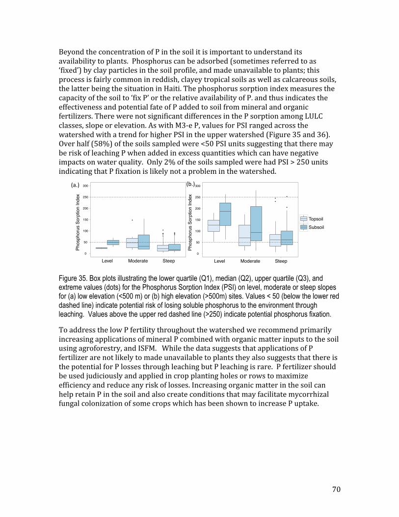
70
Beyond the concentration of P in the soil it is important to understand its availability to plants. Phosphorus can be adsorbed (sometimes referred to as ‘fixed’) by clay particles in the soil profile, and made unavailable to plants; this process is fairly common in reddish, clayey tropical soils as well as calcareous soils, the latter being the situation in Haiti. The phosphorus sorption index measures the capacity of the soil to ‘fix P’ or the relative availability of P. and thus indicates the effectiveness and potential fate of P added to soil from mineral and organic fertilizers. There were not significant differences in the P sorption among LULC classes, slope or elevation. As with M3-‐e P, values for PSI ranged across the watershed with a trend for higher PSI in the upper watershed (Figure 35 and 36). Over half (58%) of the soils sampled were <50 PSI units suggesting that there may be risk of leaching P when added in excess quantities which can have negative impacts on water quality. Only 2% of the soils sampled were had PSI > 250 units indicating that P fixation is likely not a problem in the watershed.
Figure 35. Box plots illustrating the lower quartile (Q1), median (Q2), upper quartile (Q3), and extreme values (dots) for the Phosphorus Sorption Index (PSI) on level, moderate or steep slopes for (a) low elevation (<500 m) or (b) high elevation (>500m) sites. Values < 50 (below the lower red dashed line) indicate potential risk of losing soluble phosphorus to the environment through leaching. Values above the upper red dashed line (>250) indicate potential phosphorus fixation.
To address the low P fertility throughout the watershed we recommend primarily increasing applications of mineral P combined with organic matter inputs to the soil using agroforestry, and ISFM. While the data suggests that applications of P fertilizer are not likely to made unavailable to plants they also suggests that there is the potential for P losses through leaching but P leaching is rare. P fertilizer should be used judiciously and applied in crop planting holes or rows to maximize efficiency and reduce any risk of losses. Increasing organic matter in the soil can help retain P in the soil and also create conditions that may facilitate mycorrhizal fungal colonization of some crops which has been shown to increase P uptake.
Phos
phor
us S
orpt
ion
Inde
x
0
50
100
150
200
250
300
!
!
!
!
!
!!!
Level Moderate Steep
TopsoilSubsoil
!"#$% !&#$%Ph
osph
orus
Sor
ptio
n In
dex
0
50
100
150
200
250
300
!
!
!
!
Level Moderate Steep
TopsoilSubsoil
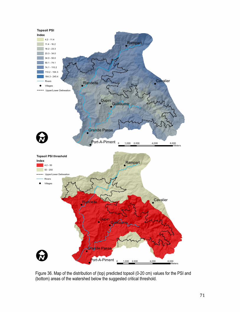
71
Figure 36. Map of the distribution of (top) predicted topsoil (0-20 cm) values for the PSI and (bottom) areas of the watershed below the suggested critical threshold.
!
!
!
!
!
!
!
Dupin
Rampart
CavalierRandelle
Guillaume
Grande Passe
Port-A-Piment 0 2,000 4,000 6,0001,000Meters
I
Topsoil PSIIndex
4.2 - 11.4
11.4 - 16.2
16.2 - 23.3
23.3 - 34.0
34.0 - 50.0
50.1 - 74.1
74.1 - 110.2
110.2 - 164.3
164.3 - 245.4
Rivers
! Villages
Upper/Lower Delineation
!
!
!
!
!
!
!
Dupin
Rampart
CavalierRandelle
Guillaume
Grande Passe
Port-A-Piment 0 2,000 4,000 6,0001,000Meters
I
Topsoil PSI thresholdIndex
4.2 - 50
50 - 250
Upper/Lower Delineation
Rivers
! Villages
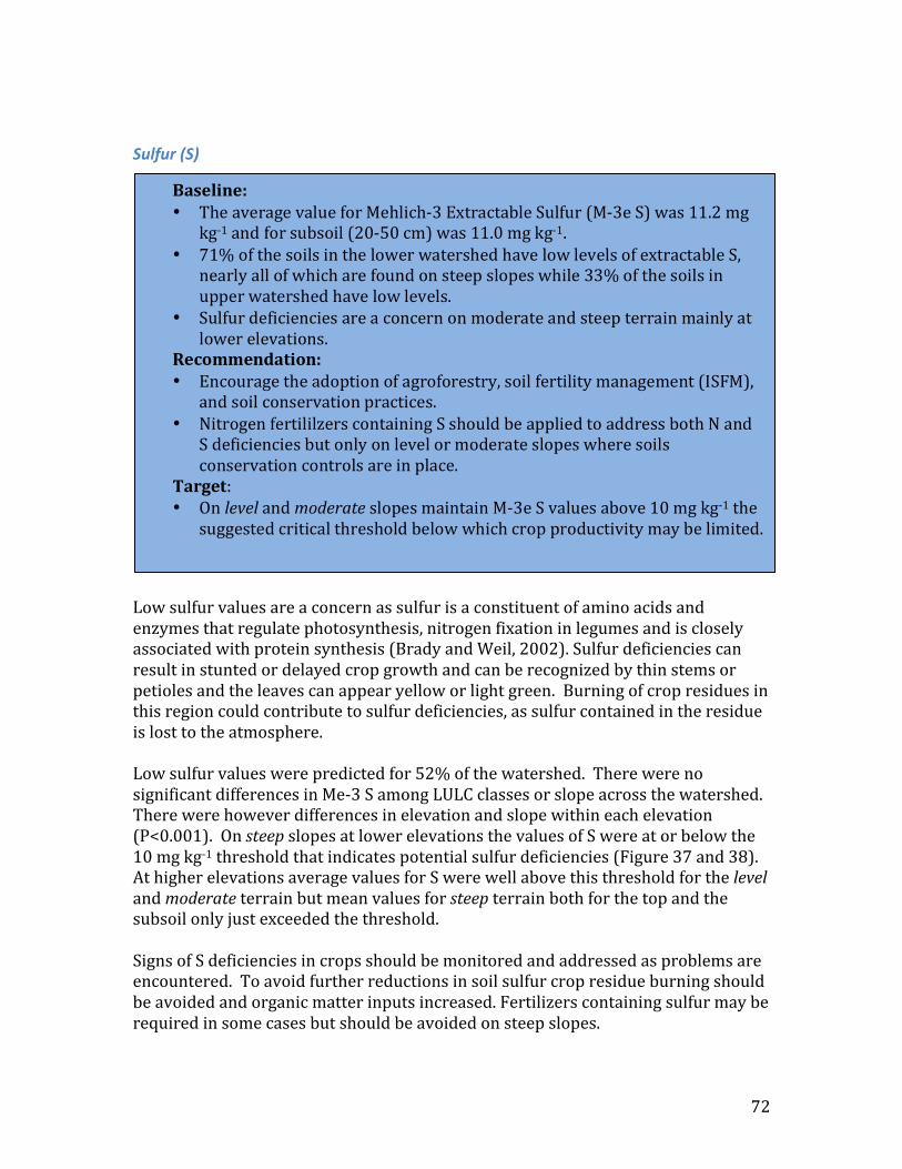
72
Sulfur (S)
Low sulfur values are a concern as sulfur is a constituent of amino acids and enzymes that regulate photosynthesis, nitrogen fixation in legumes and is closely associated with protein synthesis (Brady and Weil, 2002). Sulfur deficiencies can result in stunted or delayed crop growth and can be recognized by thin stems or petioles and the leaves can appear yellow or light green. Burning of crop residues in this region could contribute to sulfur deficiencies, as sulfur contained in the residue is lost to the atmosphere. Low sulfur values were predicted for 52% of the watershed. There were no significant differences in Me-‐3 S among LULC classes or slope across the watershed. There were however differences in elevation and slope within each elevation (P<0.001). On steep slopes at lower elevations the values of S were at or below the 10 mg kg-‐1 threshold that indicates potential sulfur deficiencies (Figure 37 and 38). At higher elevations average values for S were well above this threshold for the level and moderate terrain but mean values for steep terrain both for the top and the subsoil only just exceeded the threshold. Signs of S deficiencies in crops should be monitored and addressed as problems are encountered. To avoid further reductions in soil sulfur crop residue burning should be avoided and organic matter inputs increased. Fertilizers containing sulfur may be required in some cases but should be avoided on steep slopes.
Baseline: • The average value for Mehlich-‐3 Extractable Sulfur (M-‐3e S) was 11.2 mg
kg-‐1 and for subsoil (20-‐50 cm) was 11.0 mg kg-‐1. • 71% of the soils in the lower watershed have low levels of extractable S,
nearly all of which are found on steep slopes while 33% of the soils in upper watershed have low levels.
• Sulfur deficiencies are a concern on moderate and steep terrain mainly at lower elevations.
Recommendation: • Encourage the adoption of agroforestry, soil fertility management (ISFM),
and soil conservation practices. • Nitrogen fertililzers containing S should be applied to address both N and
S deficiencies but only on level or moderate slopes where soils conservation controls are in place.
Target: • On level and moderate slopes maintain M-‐3e S values above 10 mg kg-‐1 the
suggested critical threshold below which crop productivity may be limited.
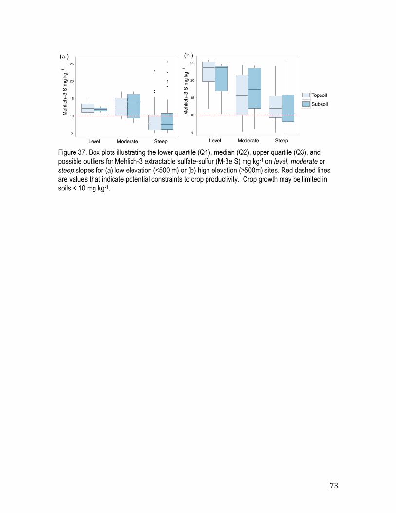
73
Figure 37. Box plots illustrating the lower quartile (Q1), median (Q2), upper quartile (Q3), and possible outliers for Mehlich-3 extractable sulfate-sulfur (M-3e S) mg kg-1 on level, moderate or steep slopes for (a) low elevation (<500 m) or (b) high elevation (>500m) sites. Red dashed lines are values that indicate potential constraints to crop productivity. Crop growth may be limited in soils < 10 mg kg-1.
!"#$% !&#$%M
ehlic
h−3
S m
g kg
!1
5
10
15
20
25
!
!
!
!
!
!
!
!
Level Moderate Steep
TopsoilSubsoil
Meh
lich−
3 S
mg
kg!1
5
10
15
20
25
Level Moderate Steep
TopsoilSubsoil
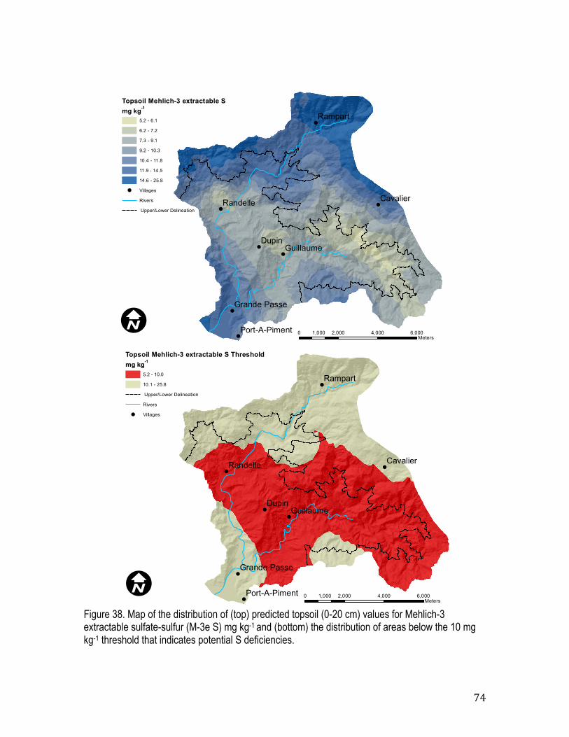
74
Figure 38. Map of the distribution of (top) predicted topsoil (0-20 cm) values for Mehlich-3 extractable sulfate-sulfur (M-3e S) mg kg-1 and (bottom) the distribution of areas below the 10 mg kg-1 threshold that indicates potential S deficiencies.
!
!
!
!
!
!
!
Dupin
Rampart
CavalierRandelle
Guillaume
Grande Passe
Port-A-Piment 0 2,000 4,000 6,0001,000Meters
I
Topsoil Mehlich-3 extractable Smg kg-1
5.2 - 6.1
6.2 - 7.2
7.3 - 9.1
9.2 - 10.3
10.4 - 11.8
11.9 - 14.5
14.6 - 25.8
! Villages
Rivers
Upper/Lower Delineation
!
!
!
!
!
!
!
Dupin
Rampart
CavalierRandelle
Guillaume
Grande Passe
Port-A-Piment 0 2,000 4,000 6,0001,000Meters
I
Topsoil Mehlich-3 extractable S Thresholdmg kg-1
5.2 - 10.0
10.1 - 25.8
Upper/Lower Delineation
Rivers
! Villages
75
Copper (Cu)
An essential component of most biochemical processes copper (Cu) enhances photosynthesis, nitrogen fixation, flowering, fruiting and maturation. Specifically it has been shown to stimulate root development, increase plant stem and stalk strength, improve flower formation and seed production, improve crop maturity, increase nitrogen fixation capacity, increase resistance to plant diseases (Fageria 2009). There were no indications of Cu limitation except for a few predicted outliers on the steep slopes of the upper watershed (Figure 39 and 40).
Figure 39. Box plots illustrating the lower quartile (Q1), median (Q2), upper quartile (Q3), and possible outliers for Mehlich-3 extractable copper (Cu) mg kg-1 on level, moderate or steep slopes for (a) low elevation (<500 m) or (b) high elevation (>500m) sites. Red dashed lines are values that indicate potential constraints to crop productivity. Crop growth may be limited in soils < 1 mg kg-1 or > 20 mg kg-1.
!"#$% !&#$%
Meh
lich−
3 C
u m
g kg
!1
0
5
10
15
20
25
!
!
!
Level Moderate Steep
TopsoilSubsoil
Meh
lich−
3 C
u m
g kg
!1
0
5
10
15
20
25
!!
!
!
!
!
!
!
Level Moderate Steep
TopsoilSubsoil
Baseline: • The average value for Mehlich-‐3 Extractable Copper (M-‐3e C) was 6.6 mg
kg-‐1 and for subsoil (20-‐50 cm) was 6.1. mg kg-‐1. • There were no potential deficiencies observed. Target: • Maintain soil M-‐3e values between 1 mg kg-‐1, the suggested critical
threshold below which crop productivity may be limited and 20 mg kg-‐1 above which toxicity may be observed.

76
Figure 40. Map of the distribution of predicted topsoil (0-20 cm) values Mehlich-3 extractable copper (Cu) mg kg-1.
Iron (Fe)
Essential for synthesizing chlorophyll, iron (Fe) is involved in nitrogen fixation and photosynthesis. Iron deficiency is often not due to insufficient iron supply, but rather iron availability. Conditions associated with that include: carbonate levels in the soil, salinity, soil moisture, low temperature, and concentration of other
!
!
!
!
!
!
!
Dupin
Rampart
CavalierRandelle
Guillaume
Grande Passe
Port-A-Piment 0 2,000 4,000 6,0001,000Meters
I
Topsoil Mehlich-3 extractable Cumg kg-1
3.6 - 4.3
4.4 - 4.9
5.0 - 5.7
5.8 - 6.8
6.9 - 7.9
8.0 - 9.0
9.1 - 20.2
! Villages
Rivers
Upper/Lower Delineation
Baseline: • The average value for Mehlich-‐3 Extractable Iron (M-‐3e Fe) was 166.8 mg
kg-‐1 and for subsoil (20-‐50 cm) 166.5mg kg-‐1 and therefore does not appear to be deficient or at toxic levels for crop growth.
Target: • Maintain soil concentrations between 50 mg kg-‐1 below which may
indicate Fe deficiencies and 200 mg kg-‐1 above which soils may fix P.
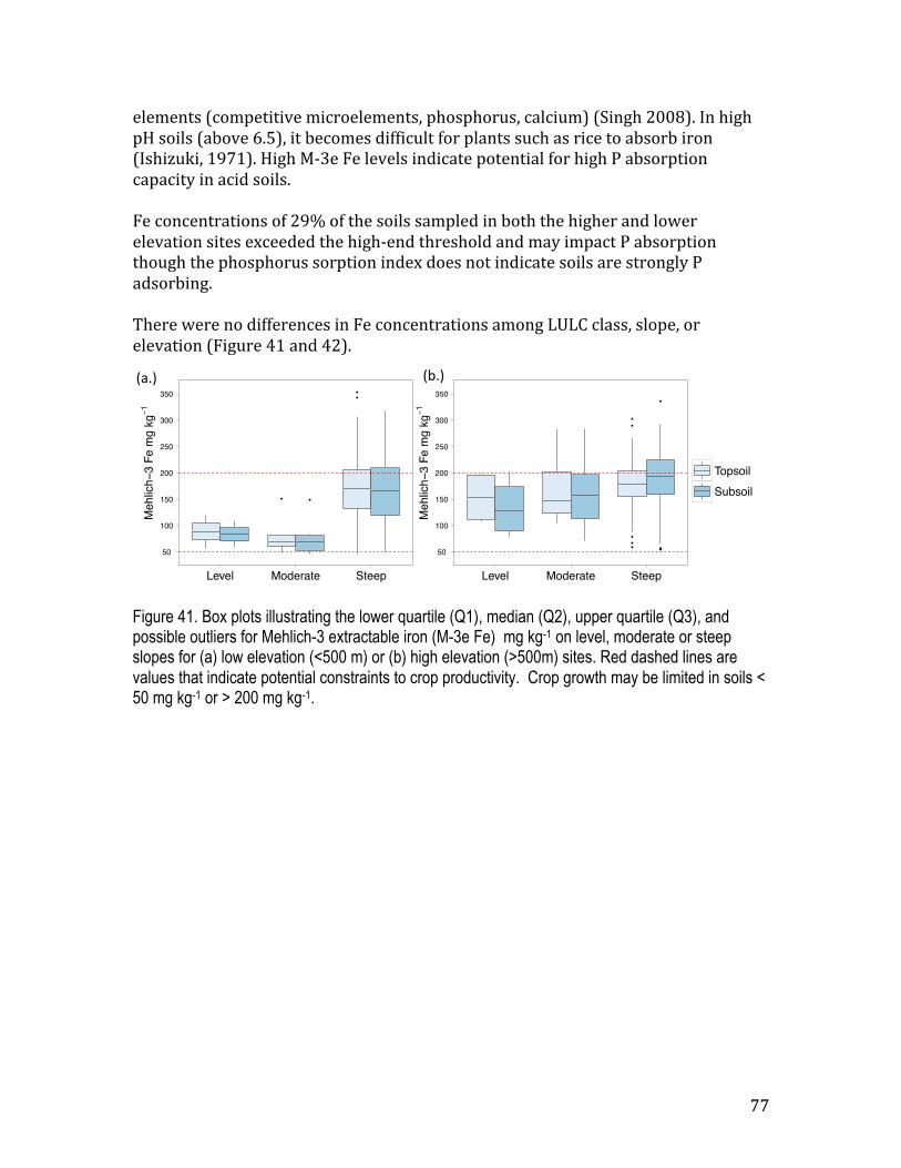
77
elements (competitive microelements, phosphorus, calcium) (Singh 2008). In high pH soils (above 6.5), it becomes difficult for plants such as rice to absorb iron (Ishizuki, 1971). High M-‐3e Fe levels indicate potential for high P absorption capacity in acid soils. Fe concentrations of 29% of the soils sampled in both the higher and lower elevation sites exceeded the high-‐end threshold and may impact P absorption though the phosphorus sorption index does not indicate soils are strongly P adsorbing. There were no differences in Fe concentrations among LULC class, slope, or elevation (Figure 41 and 42).
Figure 41. Box plots illustrating the lower quartile (Q1), median (Q2), upper quartile (Q3), and possible outliers for Mehlich-3 extractable iron (M-3e Fe) mg kg-1 on level, moderate or steep slopes for (a) low elevation (<500 m) or (b) high elevation (>500m) sites. Red dashed lines are values that indicate potential constraints to crop productivity. Crop growth may be limited in soils < 50 mg kg-1 or > 200 mg kg-1.
!"#$% !&#$%
Meh
lich−
3 Fe
mg
kg!1
50
100
150
200
250
300
350
! !
!
!
Level Moderate Steep
TopsoilSubsoil
Meh
lich−
3 Fe
mg
kg!1
50
100
150
200
250
300
350
!
!
!
!
!
!
!!!
Level Moderate Steep
TopsoilSubsoil
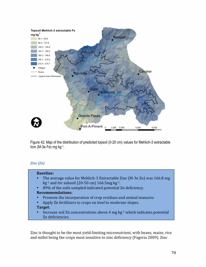
78
Figure 42. Map of the distribution of predicted topsoil (0-20 cm) values for Mehlich-3 extractable Iron (M-3e Fe) mg kg-1.
Zinc (Zn)
Zinc is thought to be the most yield-‐limiting micronutrient, with beans, maize, rice and millet being the crops most sensitive to zinc deficiency (Fageria 2009). Zinc
!
!
!
!
!
!
!
Dupin
Rampart
CavalierRandelle
Guillaume
Grande Passe
Port-A-Piment 0 2,000 4,000 6,0001,000Meters
I
Topsoil Mehlich-3 extractable Femg kg-1
59.1 - 90.8
90.9 - 127.9
128.0 - 154.6
154.7 - 180.2
180.3 - 195.0
195.1 - 210.3
210.4 - 370.7
! Villages
Rivers
Upper/Lower Delineation
Baseline: • The average value for Mehlich-‐3 Extractable Zinc (M-‐3e Zn) was 166.8 mg
kg-‐1 and for subsoil (20-‐50 cm) 166.5mg kg-‐1. • 89% of the soils sampled indicated potential Zn deficiency. Recommendations: • Promote the incorporation of crop residues and animal manures • Apply Zn fertilizers to crops on level to moderate slopes. Target: • Increase soil Zn concentrations above 4 mg kg-‐1 which indicates potential
Zn deficiencies.
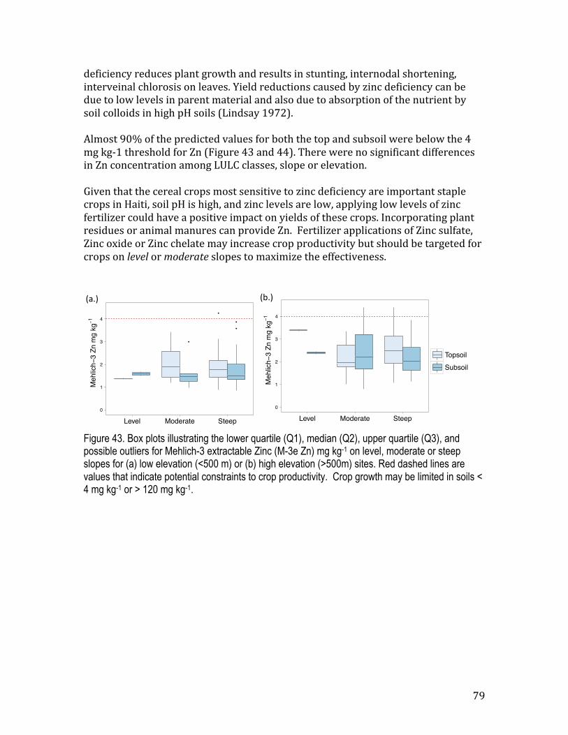
79
deficiency reduces plant growth and results in stunting, internodal shortening, interveinal chlorosis on leaves. Yield reductions caused by zinc deficiency can be due to low levels in parent material and also due to absorption of the nutrient by soil colloids in high pH soils (Lindsay 1972). Almost 90% of the predicted values for both the top and subsoil were below the 4 mg kg-‐1 threshold for Zn (Figure 43 and 44). There were no significant differences in Zn concentration among LULC classes, slope or elevation. Given that the cereal crops most sensitive to zinc deficiency are important staple crops in Haiti, soil pH is high, and zinc levels are low, applying low levels of zinc fertilizer could have a positive impact on yields of these crops. Incorporating plant residues or animal manures can provide Zn. Fertilizer applications of Zinc sulfate, Zinc oxide or Zinc chelate may increase crop productivity but should be targeted for crops on level or moderate slopes to maximize the effectiveness.
Figure 43. Box plots illustrating the lower quartile (Q1), median (Q2), upper quartile (Q3), and possible outliers for Mehlich-3 extractable Zinc (M-3e Zn) mg kg-1 on level, moderate or steep slopes for (a) low elevation (<500 m) or (b) high elevation (>500m) sites. Red dashed lines are values that indicate potential constraints to crop productivity. Crop growth may be limited in soils < 4 mg kg-1 or > 120 mg kg-1.
!"#$% !&#$%
Meh
lich−
3 Zn
mg
kg!1
0
1
2
3
4
!
!
!
!
Level Moderate Steep
TopsoilSubsoil
Meh
lich−
3 Zn
mg
kg!1
0
1
2
3
4
Level Moderate Steep
TopsoilSubsoil
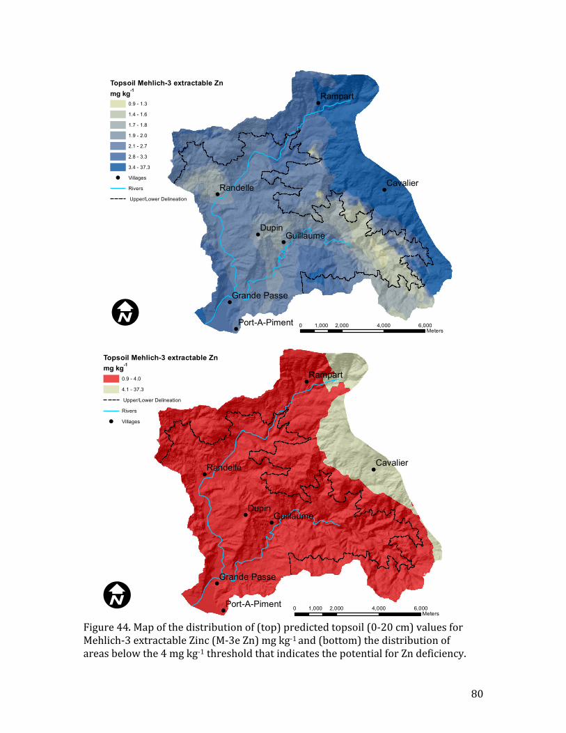
80
Figure 44. Map of the distribution of (top) predicted topsoil (0-‐20 cm) values for Mehlich-‐3 extractable Zinc (M-‐3e Zn) mg kg-‐1 and (bottom) the distribution of areas below the 4 mg kg-‐1 threshold that indicates the potential for Zn deficiency.
!
!
!
!
!
!
!
Dupin
Rampart
CavalierRandelle
Guillaume
Grande Passe
Port-A-Piment 0 2,000 4,000 6,0001,000Meters
I
Topsoil Mehlich-3 extractable Znmg kg-1
0.9 - 1.3
1.4 - 1.6
1.7 - 1.8
1.9 - 2.0
2.1 - 2.7
2.8 - 3.3
3.4 - 37.3
! Villages
Rivers
Upper/Lower Delineation
!
!
!
!
!
!
!
Dupin
Rampart
CavalierRandelle
Guillaume
Grande Passe
Port-A-Piment 0 2,000 4,000 6,0001,000Meters
I
Topsoil Mehlich-3 extractable Znmg kg-1
0.9 - 4.0
4.1 - 37.3
Upper/Lower Delineation
Rivers
! Villages
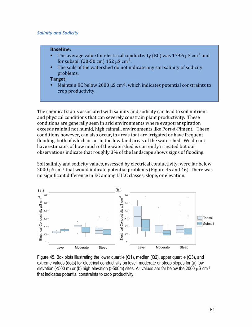
81
Salinity and Sodicity
The chemical status associated with salinity and sodicity can lead to soil nutrient and physical conditions that can severely constrain plant productivity. These conditions are generally seen in arid environments where evapotranspiration exceeds rainfall not humid, high rainfall, environments like Port-‐à-‐Piment. These conditions however, can also occur, in areas that are irrigated or have frequent flooding, both of which occur in the low-‐land areas of the watershed. We do not have estimates of how much of the watershed is currently irrigated but our observations indicate that roughly 3% of the landscape shows signs of flooding. Soil salinity and sodicity values, assessed by electrical conductivity, were far below 2000 µS cm-‐1 that would indicate potential problems (Figure 45 and 46). There was no significant difference in EC among LULC classes, slope, or elevation.
Figure 45. Box plots illustrating the lower quartile (Q1), median (Q2), upper quartile (Q3), and extreme values (dots) for electrical conductivity on level, moderate or steep slopes for (a) low elevation (<500 m) or (b) high elevation (>500m) sites. All values are far below the 2000 µS cm-1
that indicates potential constraints to crop productivity.
!"#$% !&#$%
Elec
trica
l Con
duct
ivity
µS
cm!1
0
100
200
300
400
500
600
!
!
!
!!
!
!
!
Level Moderate Steep
TopsoilSubsoil
Elec
trica
l Con
duct
ivity
µS
cm!1
0
100
200
300
400
500
600!
!
!
!
!
!
!
Level Moderate Steep
TopsoilSubsoil
Baseline: • The average value for electrical conductivity (EC) was 179.6 µS cm-1 and
for subsoil (20-‐50 cm) 152 µS cm-1. • The soils of the watershed do not indicate any soil salinity of sodicity
problems. Target: • Maintain EC below 2000 μS cm-‐1, which indicates potential constraints to
crop productivity.
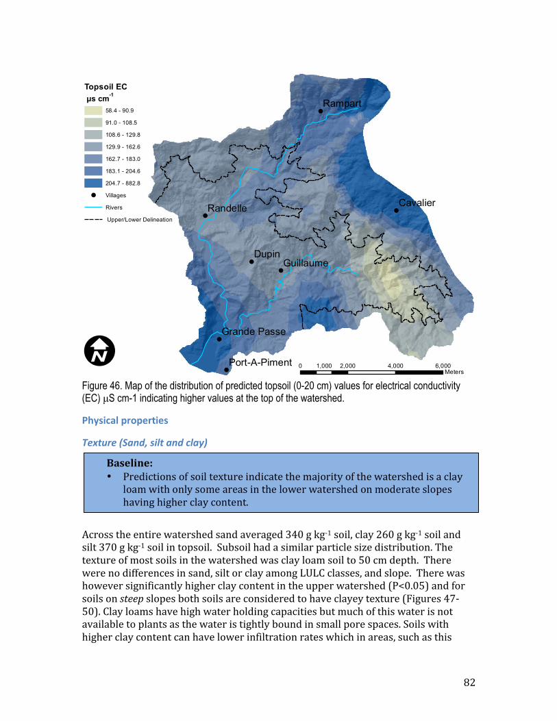
82
Figure 46. Map of the distribution of predicted topsoil (0-20 cm) values for electrical conductivity (EC) µS cm-1 indicating higher values at the top of the watershed.
Physical properties
Texture (Sand, silt and clay)
Across the entire watershed sand averaged 340 g kg-‐1 soil, clay 260 g kg-‐1 soil and silt 370 g kg-‐1 soil in topsoil. Subsoil had a similar particle size distribution. The texture of most soils in the watershed was clay loam soil to 50 cm depth. There were no differences in sand, silt or clay among LULC classes, and slope. There was however significantly higher clay content in the upper watershed (P<0.05) and for soils on steep slopes both soils are considered to have clayey texture (Figures 47-‐50). Clay loams have high water holding capacities but much of this water is not available to plants as the water is tightly bound in small pore spaces. Soils with higher clay content can have lower infiltration rates which in areas, such as this
!
!
!
!
!
!
!
Dupin
Rampart
CavalierRandelle
Guillaume
Grande Passe
Port-A-Piment 0 2,000 4,000 6,0001,000Meters
I
58.4 - 90.9
91.0 - 108.5
108.6 - 129.8
129.9 - 162.6
162.7 - 183.0
183.1 - 204.6
204.7 - 882.8
! Villages
Rivers
Upper/Lower Delineation
Baseline: • Predictions of soil texture indicate the majority of the watershed is a clay
loam with only some areas in the lower watershed on moderate slopes having higher clay content.
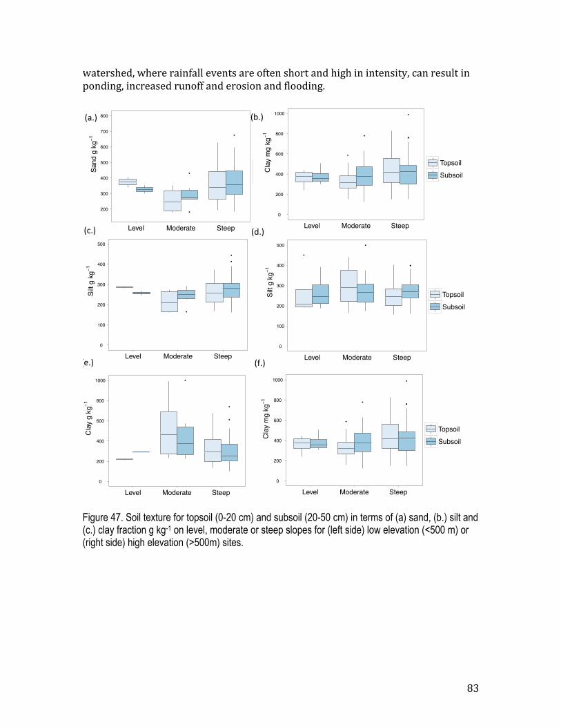
83
watershed, where rainfall events are often short and high in intensity, can result in ponding, increased runoff and erosion and flooding.
Figure 47. Soil texture for topsoil (0-20 cm) and subsoil (20-50 cm) in terms of (a) sand, (b.) silt and (c.) clay fraction g kg-1 on level, moderate or steep slopes for (left side) low elevation (<500 m) or (right side) high elevation (>500m) sites.
Cla
y g
kg!1
0
200
400
600
800
1000 !
!
!
Level Moderate Steep
TopsoilSubsoil
Cla
y m
g kg
!1
0
200
400
600
800
1000
!
!
!
!
!
Level Moderate Steep
TopsoilSubsoil
Silt
g kg
!1
0
100
200
300
400
500
!
!
!
Level Moderate Steep
TopsoilSubsoil
Silt
g kg
!1
0
100
200
300
400
500
!
!
!!
Level Moderate Steep
TopsoilSubsoil
Sand
g k
g!1
200
300
400
500
600
700
800
!
!
!
Level Moderate Steep
TopsoilSubsoil
Cla
y m
g kg
!1
0
200
400
600
800
1000
!
!
!
!
!
Level Moderate Steep
TopsoilSubsoil
!"#$% !&#$%
!'#$% !(#$%
!)#$% !*#$%
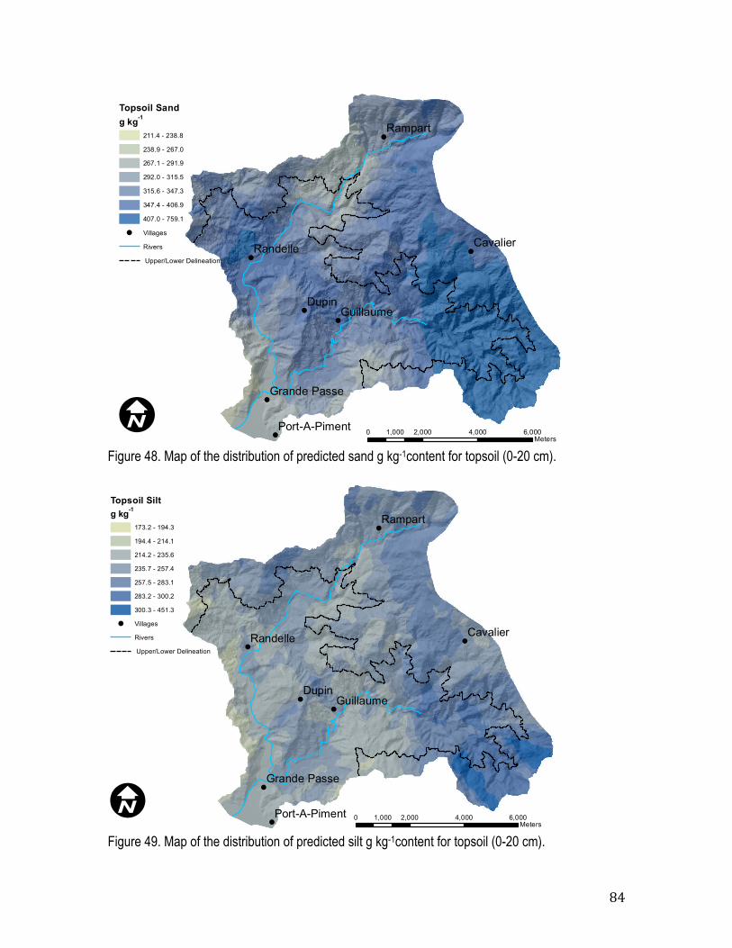
84
Figure 48. Map of the distribution of predicted sand g kg-1content for topsoil (0-20 cm).
Figure 49. Map of the distribution of predicted silt g kg-1content for topsoil (0-20 cm).
!
!
!
!
!
!
!
Dupin
Rampart
CavalierRandelle
Guillaume
Grande Passe
Port-A-Piment 0 2,000 4,000 6,0001,000Meters
I
Topsoil Siltg kg-1
173.2 - 194.3
194.4 - 214.1
214.2 - 235.6
235.7 - 257.4
257.5 - 283.1
283.2 - 300.2
300.3 - 451.3
! Villages
Rivers
Upper/Lower Delineation
!
!
!
!
!
!
!
Dupin
Rampart
CavalierRandelle
Guillaume
Grande Passe
Port-A-Piment 0 2,000 4,000 6,0001,000Meters
I
Topsoil Sandg kg-1
211.4 - 238.8
238.9 - 267.0
267.1 - 291.9
292.0 - 315.5
315.6 - 347.3
347.4 - 406.9
407.0 - 759.1
! Villages
Rivers
Upper/Lower Delineation
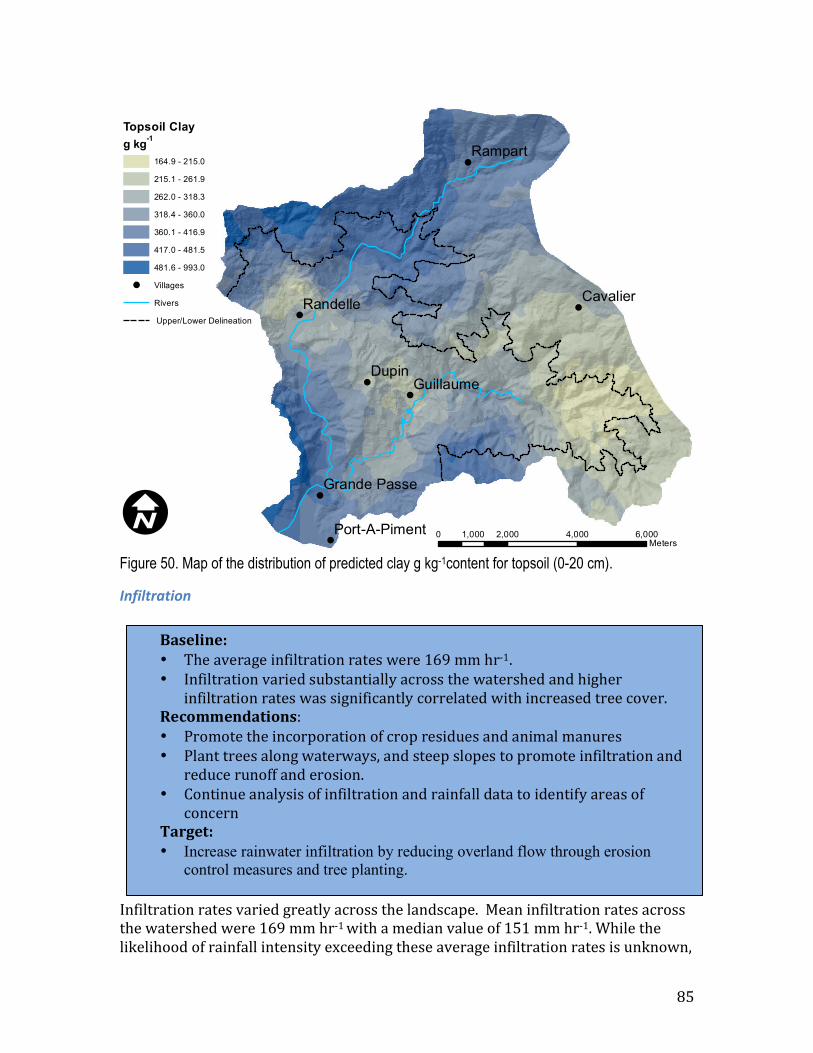
85
Figure 50. Map of the distribution of predicted clay g kg-1content for topsoil (0-20 cm).
Infiltration
Infiltration rates varied greatly across the landscape. Mean infiltration rates across the watershed were 169 mm hr-‐1 with a median value of 151 mm hr-‐1. While the likelihood of rainfall intensity exceeding these average infiltration rates is unknown,
!
!
!
!
!
!
!
Dupin
Rampart
CavalierRandelle
Guillaume
Grande Passe
Port-A-Piment 0 2,000 4,000 6,0001,000Meters
I
Topsoil Clayg kg-1
164.9 - 215.0
215.1 - 261.9
262.0 - 318.3
318.4 - 360.0
360.1 - 416.9
417.0 - 481.5
481.6 - 993.0
! Villages
Rivers
Upper/Lower Delineation
Baseline: • The average infiltration rates were 169 mm hr-‐1. • Infiltration varied substantially across the watershed and higher
infiltration rates was significantly correlated with increased tree cover. Recommendations: • Promote the incorporation of crop residues and animal manures • Plant trees along waterways, and steep slopes to promote infiltration and
reduce runoff and erosion. • Continue analysis of infiltration and rainfall data to identify areas of
concern Target: • Increase rainwater infiltration by reducing overland flow through erosion
control measures and tree planting.
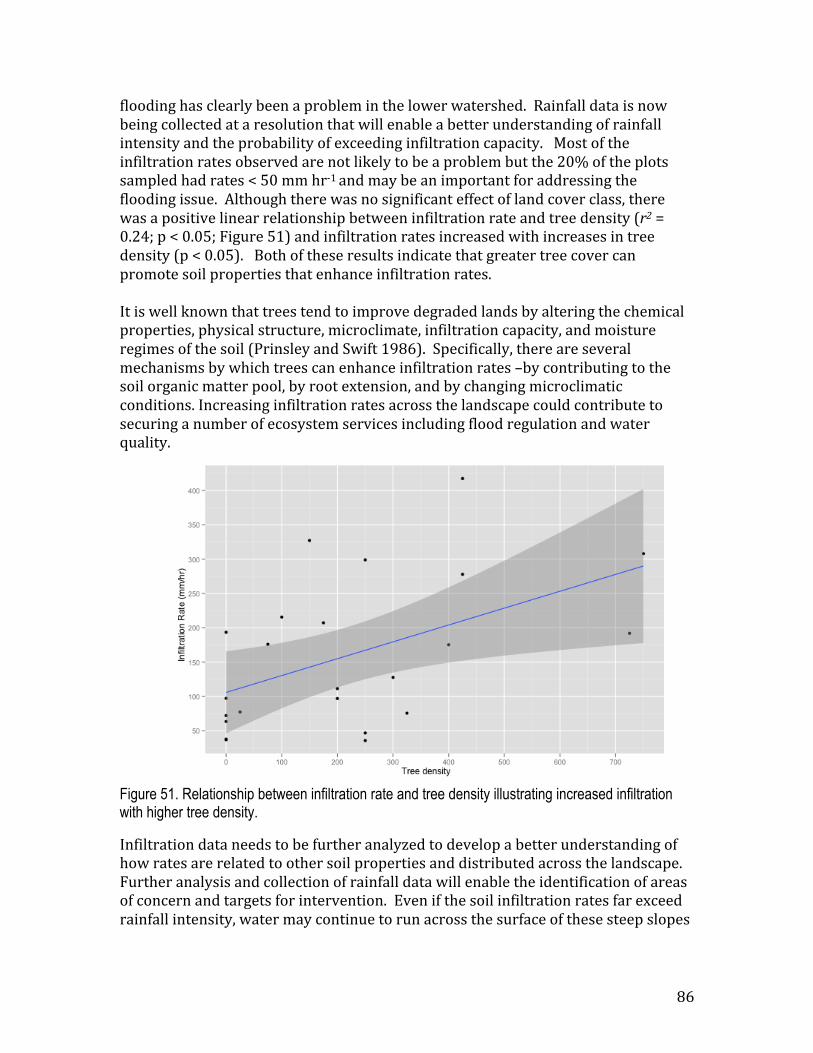
86
flooding has clearly been a problem in the lower watershed. Rainfall data is now being collected at a resolution that will enable a better understanding of rainfall intensity and the probability of exceeding infiltration capacity. Most of the infiltration rates observed are not likely to be a problem but the 20% of the plots sampled had rates < 50 mm hr-‐1 and may be an important for addressing the flooding issue. Although there was no significant effect of land cover class, there was a positive linear relationship between infiltration rate and tree density (r2 = 0.24; p < 0.05; Figure 51) and infiltration rates increased with increases in tree density (p < 0.05). Both of these results indicate that greater tree cover can promote soil properties that enhance infiltration rates. It is well known that trees tend to improve degraded lands by altering the chemical properties, physical structure, microclimate, infiltration capacity, and moisture regimes of the soil (Prinsley and Swift 1986). Specifically, there are several mechanisms by which trees can enhance infiltration rates –by contributing to the soil organic matter pool, by root extension, and by changing microclimatic conditions. Increasing infiltration rates across the landscape could contribute to securing a number of ecosystem services including flood regulation and water quality.
Figure 51. Relationship between infiltration rate and tree density illustrating increased infiltration with higher tree density.
Infiltration data needs to be further analyzed to develop a better understanding of how rates are related to other soil properties and distributed across the landscape. Further analysis and collection of rainfall data will enable the identification of areas of concern and targets for intervention. Even if the soil infiltration rates far exceed rainfall intensity, water may continue to run across the surface of these steep slopes
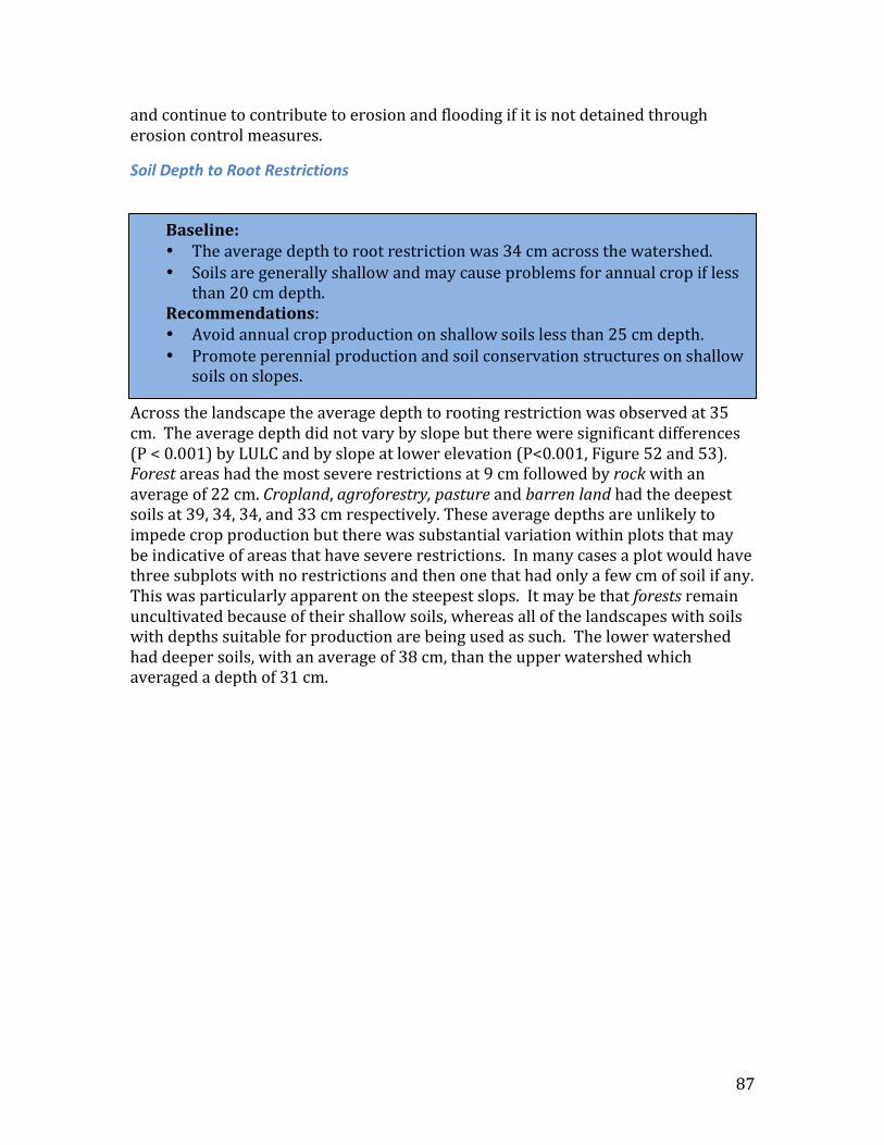
87
and continue to contribute to erosion and flooding if it is not detained through erosion control measures.
Soil Depth to Root Restrictions
Across the landscape the average depth to rooting restriction was observed at 35 cm. The average depth did not vary by slope but there were significant differences (P < 0.001) by LULC and by slope at lower elevation (P<0.001, Figure 52 and 53). Forest areas had the most severe restrictions at 9 cm followed by rock with an average of 22 cm. Cropland, agroforestry, pasture and barren land had the deepest soils at 39, 34, 34, and 33 cm respectively. These average depths are unlikely to impede crop production but there was substantial variation within plots that may be indicative of areas that have severe restrictions. In many cases a plot would have three subplots with no restrictions and then one that had only a few cm of soil if any. This was particularly apparent on the steepest slops. It may be that forests remain uncultivated because of their shallow soils, whereas all of the landscapes with soils with depths suitable for production are being used as such. The lower watershed had deeper soils, with an average of 38 cm, than the upper watershed which averaged a depth of 31 cm. 5 .12. Shallow depth (R)
Baseline: • The average depth to root restriction was 34 cm across the watershed. • Soils are generally shallow and may cause problems for annual crop if less
than 20 cm depth. Recommendations: • Avoid annual crop production on shallow soils less than 25 cm depth. • Promote perennial production and soil conservation structures on shallow
soils on slopes.
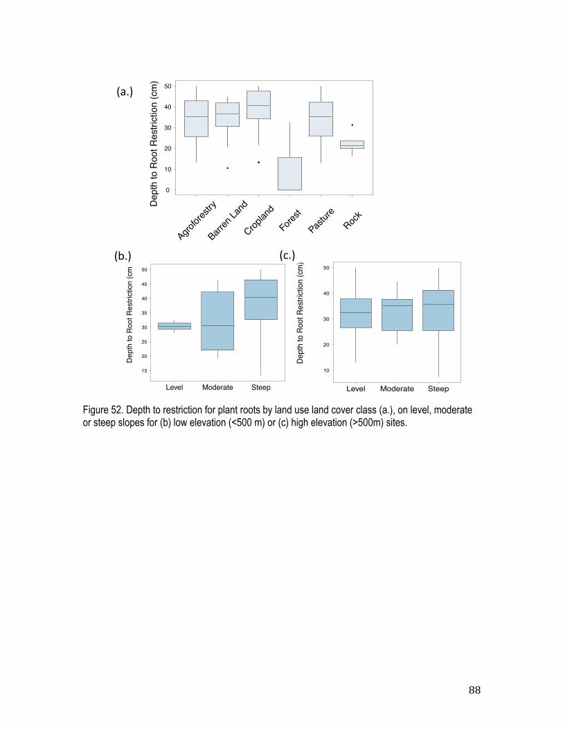
88
Figure 52. Depth to restriction for plant roots by land use land cover class (a.), on level, moderate or steep slopes for (b) low elevation (<500 m) or (c) high elevation (>500m) sites.
D
epth
to R
oot R
estri
ctio
n (c
m)
15
20
25
30
35
40
45
50
Level Moderate Steep
De
pth
to R
oot R
estri
ctio
n (c
m)
10
20
30
40
50
Level Moderate Steep
!"#$%
!&#$% !'#$%
D
epth
to R
oot R
estri
ctio
n (c
m)
0
10
20
30
40
50
!
!!
!
Agrofor
estry
Barren
Land
Croplan
d
Fores
t
Pastur
eRoc
k
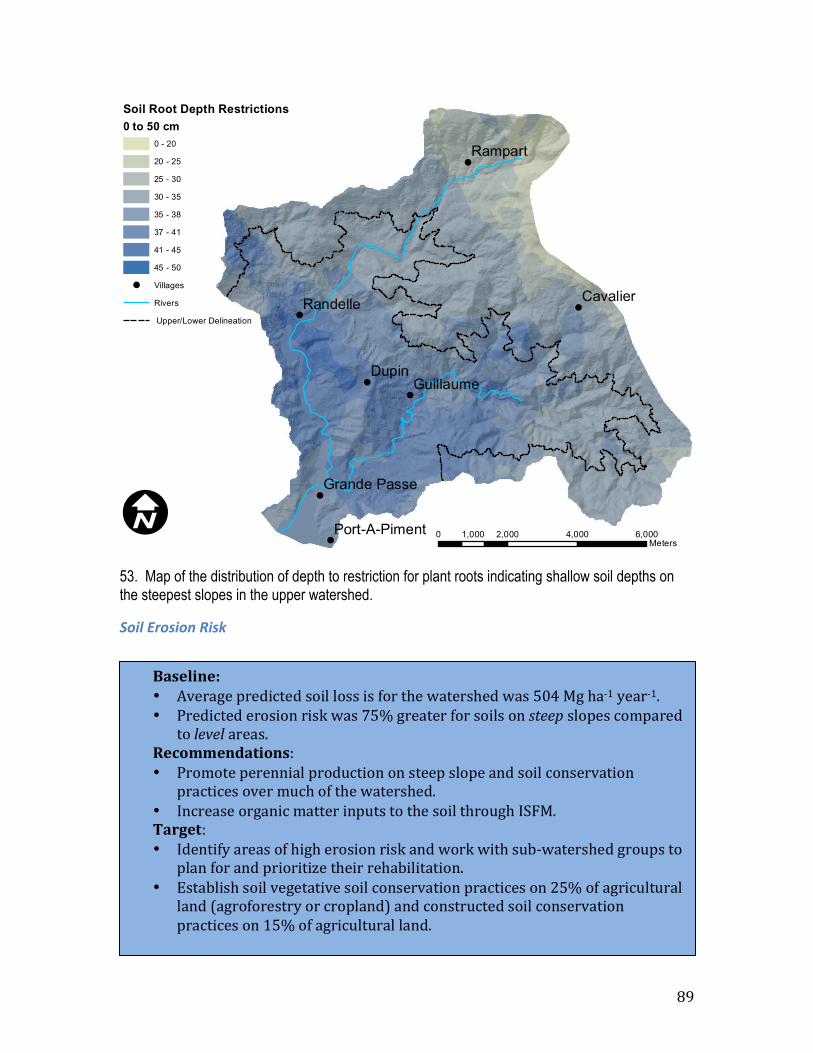
89
53. Map of the distribution of depth to restriction for plant roots indicating shallow soil depths on the steepest slopes in the upper watershed.
Soil Erosion Risk
!
!
!
!
!
!
!
Dupin
Rampart
CavalierRandelle
Guillaume
Grande Passe
Port-A-Piment 0 2,000 4,000 6,0001,000Meters
I
Soil Root Depth Restrictions0 to 50 cm
0 - 20
20 - 25
25 - 30
30 - 35
35 - 38
37 - 41
41 - 45
45 - 50
! Villages
Rivers
Upper/Lower Delineation
Baseline: • Average predicted soil loss is for the watershed was 504 Mg ha-‐1 year-‐1. • Predicted erosion risk was 75% greater for soils on steep slopes compared
to level areas. Recommendations: • Promote perennial production on steep slope and soil conservation
practices over much of the watershed. • Increase organic matter inputs to the soil through ISFM. Target: • Identify areas of high erosion risk and work with sub-‐watershed groups to
plan for and prioritize their rehabilitation. • Establish soil vegetative soil conservation practices on 25% of agricultural
land (agroforestry or cropland) and constructed soil conservation practices on 15% of agricultural land.
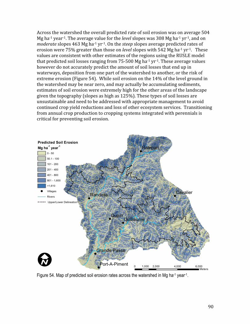
90
Across the watershed the overall predicted rate of soil erosion was on average 504 Mg ha-‐1 year-‐1. The average value for the level slopes was 308 Mg ha-‐1 yr-‐1, and on moderate slopes 463 Mg ha-‐1 yr-‐1. On the steep slopes average predicted rates of erosion were 75% greater than those on level slopes with 542 Mg ha-‐1 yr-‐1. These values are consistent with other estimates of the regions using the RUSLE model that predicted soil losses ranging from 75-‐500 Mg ha-‐1 yr-‐1. These average values however do not accurately predict the amount of soil losses that end up in waterways, deposition from one part of the watershed to another, or the risk of extreme erosion (Figure 54). While soil erosion on the 14% of the level ground in the watershed may be near zero, and may actually be accumulating sediments, estimates of soil erosion were extremely high for the other areas of the landscape given the topography (slopes as high as 125%). These types of soil losses are unsustainable and need to be addressed with appropriate management to avoid continued crop yield reductions and loss of other ecosystem services. Transitioning from annual crop production to cropping systems integrated with perennials is critical for preventing soil erosion.
Figure 54. Map of predicted soil erosion rates across the watershed in Mg ha-1 year-1.
!
!
!
!
!
!
!
Dupin
Rampart
CavalierRandelle
Guillaume
Grande Passe
Port-A-Piment 0 2,000 4,000 6,0001,000Meters
I
Predicted Soil ErosionMg ha-1 year-1
0 - 50
50.1 - 100
101 - 200
201 - 400
401 - 800
801 - 1,600
>1,610
! Villages
Rivers
Upper/Lower Delineation
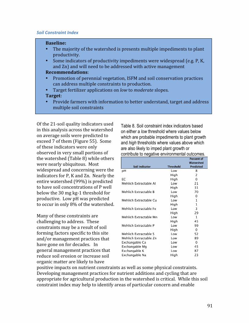
91
Soil Constraint Index
Of the 21-‐soil quality indicators used in this analysis across the watershed on average soils were predicted to exceed 7 of them (Figure 55). Some of these indicators were only observed in very small portions of the watershed (Table 8) while others were nearly ubiquitous. Most widespread and concerning were the indicators for P, K and Zn. Nearly the entire watershed (99%) is predicted to have soil concentrations of P well below the 30 mg kg-‐1 threshold for productive. Low pH was predicted to occur in only 8% of the watershed. Many of these constraints are challenging to address. These constraints may be a result of soil forming factors specific to this site and/or management practices that have gone on for decades. In general management practices that reduce soil erosion or increase soil organic matter are likely to have positive impacts on nutrient constraints as well as some physical constraints. Developing management practices for nutrient additions and cycling that are appropriate for agricultural production in the watershed is critical. While this soil constraint index may help to identify areas of particular concern and enable
Baseline: • The majority of the watershed is presents multiple impediments to plant
productivity. • Some indicators of productivity impediments were widespread (e.g. P, K,
and Zn) and will need to be addressed with active management Recommendations: • Promotion of perennial vegetation, ISFM and soil conservation practices
can address multiple constraints to production. • Target fertilizer applications on low to moderate slopes. Target: • Provide farmers with information to better understand, target and address
multiple soil constraints
Table 8. Soil constraint index indicators based on either a low threshold where values below which are probable impediments to plant growth and high thresholds where values above which are also likely to imped plant growth or contribute to negative environmental outcomes.
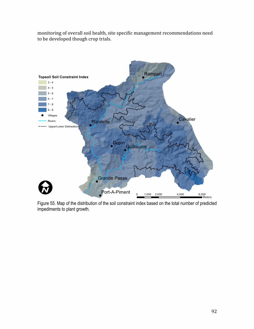
92
monitoring of overall soil health, site specific management recommendations need to be developed though crop trials.
Figure 55. Map of the distribution of the soil constraint index based on the total number of predicted impediments to plant growth.
!
!
!
!
!
!
!
Dupin
Rampart
CavalierRandelle
Guillaume
Grande Passe
Port-A-Piment 0 2,000 4,000 6,0001,000Meters
I
Topsoil Soil Constraint Index3 - 4
4 - 5
5 - 6
6 - 7
7 - 8
8 - 9
! Villages
Rivers
Upper/Lower Delineation
93
Major Findings, Recommendations and Next Steps The steep slopes of the Port-‐à-‐Piment watershed are almost entirely utilized for agricultural production most of which is annual cropping. Only 14% of the total landscape is covered in woody vegetation, either trees or shrubs, and of this only 5% is closed canopy forest. The analysis of the distribution of slopes throughout the watershed shows that only 14% of the area is considered level (0-‐16% slope) and suitable for annual cropping with nutrient inputs or irrigation without substantial investment in soil conservation practices. Moderate slopes (16-‐30%) constitute 23% of the landscape. These slopes may be productive for annual cropping but failing to employ soil conservation practices will be at risk of erosion of soil and nutrients. The majority of the slopes in the watershed, nearly 64%, are considered steep (30-‐130%) and are inappropriate for annual cropping. These slopes are at significant risk of erosion if left bare for any period of the rainy season. There is substantial evidence of severe erosion throughout the watershed. Gully erosion was observed on 22% of the landscape, found mainly on steep slopes and in cropland. All across the watershed topsoil has eroded, and therefore soils are low in soil organic matter and nitrogen. There is likely substantial potential to increase soil organic matter in cropland and thus improve soil fertility and other ecosystem services. pH is generally within a range that will not limit most plant productivity, though soils at higher elevations have lower pH and may require trees and crops adapted for more acidic conditions such as coffee. The analysis suggest that although the capacity to hold nutrients is high in terms of CEC, those most critical for production N, P, and K are likely limited. The soils do have fairly high concentrations of Ca, but Mg may be limiting to crop production in some parts of the watershed. There are no indications that the micronutrients Cu or Fe are limiting plant growth in the watershed but S, and Zn may be problematic in most parts of the watershed. Analyses did not indicate any soil salinity or sodicity issues. Predictions of soil texture indicate the majority of the watershed is a clay loam with only some areas in the lower watershed on moderate slopes having higher clay content. Predictions of soil depth suggest that restrictions (< 10 cm) for plant roots are found mainly on steep slopes. Water infiltration was correlated positively with increased tree cover so increased tree cover would result in more water entering the soil and less water runoff eroding the hillsides.
Key Problems The most important problem to address in the Port-‐à-‐Piment watershed is the widespread and large-‐scale soil erosion. Erosion caused by annual cropping, intense rainfall and lack of perennial vegetation on steep slopes must be addressed. Predictions for soil erosion indicates that slopes >30% are likely to have soil losses >500 Mg ha-‐1 yr-‐1, a rate which cannot sustain plant production for agriculture or forestry. Many of the key problems observed in the watershed are related to and/or exacerbated by this rate of erosion. The key problems that need to be addressed in order to secure multiple ecosystem services:
• Forests cover is only 5% of the landscape
94
• There were no soil conservation practices observed across the watershed and annual production dominates even the steepest slopes.
• The majority of the watershed is predicted to have a multiple impediments to plant productivity; the highest number of constraints is predicted to be in the southeastern region of the watershed and in a band across the middle elevations.
• The majority of the soils in the watershed are likely deficient in N,P,K and Zn. • The PSI indicates much of the lower watershed could be a problem for P
absorption • S and Mg are likely to be limiting for plant productivity in some parts of the
watershed.
Recommendations There needs to be widespread changes in land management to meet objectives of increasing farmer income and improving the environmental sustainability of the watershed. Strategies to meet these objectives should be developed by all the stakeholders involved in a way that enables an understanding of various options and their associated outcomes in both the near and long-‐term. The information provided by this analysis can help inform such strategy development but the multiple factors in the data are challenging to interpret and could be overwhelming to address factor by factor. Below we suggest simple guidelines for using the information for targeting management recommendations to address some of the key soil problems identified in this study. Some of guidelines can be followed using visual characteristics of the landscape and do not require the extensive list of soil data; this approach is possible from the synthesis provided in this report. Numerous methods have been developed for land use classification to help with this type of planning. Two of the most widely used approaches are the USDA land capability classification system (LCC) (Klingebiel and Montgomery 1961) the FAO land evaluation framework (FAO 1976). Both methods consider soil erosion risk as a determining factor and have been adapted for different countries in the world. However, some researchers argue that the LCC system completely ignores economic factors and specific uses of land, and may not be appropriate for developing countries (Van Diepen et al. 1991). Thus, other land capability systems were proposed to be more applicable for use on hilly marginal lands (Sheng 1971, Hudson 1977, Gumbs 1997). Classifications of land use types (LUT) when possible should be appropriate for the site-‐specific biophysical and socioeconomic conditions. Given Haiti’s land constraints, high levels of poverty, and extreme topography, strategies must be developed for Haiti that balance the need to produce economic returns on marginal lands while protecting the long-‐term availability of ecosystem services. In the Port-‐a-‐Piment watershed 88% of crop production is on slopes > 30%; while these lands are not likely to be very productive they are a critical component of livelihood strategies and land use planning must address this.
95
The data presented here can provide a basis for formulating management options and in combination with continued data collection and analysis, will help monitor outcomes at the field to watershed scale. We propose that developing a basic land use decision tree that can be understood and agreed upon by stakeholders will facilitate the adoption of management practices that will meet the broadest needs. A first draft of a basic decision tree is presented in this report to begin this consultative effort and provide a basic set of recommendations that if implemented, will help achieve project objectives. Here we present the framework for the decision tree and how it would be used in conjunction with the digital maps and crop information we provide. These recommendations are based on the precautionary principle; in the absence of perfect information a conservative recommendation is made to avoid actions or policies that have suspected risks of causing harm. The decision tree (see Figure 56) is divided into four basic nodes for making land management recommendations. At each of the nodes, there are key questions, which lead to the next node. Working through these questions will lead to site-‐specific recommendations for management, either for crop, pasture or some type of perennial production classified into distinct systems appropriate for the site i.e. 1-‐4. Perennial production would include trees and shrubs planted primarily for woodfuel, timber, fruit or nuts, soil conservation, riverbank stabilization, shade (i.e. for coffee), fodder or more appropriately a combination of these. For each of the crop production options an associated set of site-‐specific soil management recommendations are presented. The following is a schematic and description of each of the basic nodes, and associated production priorities and soil management practices.
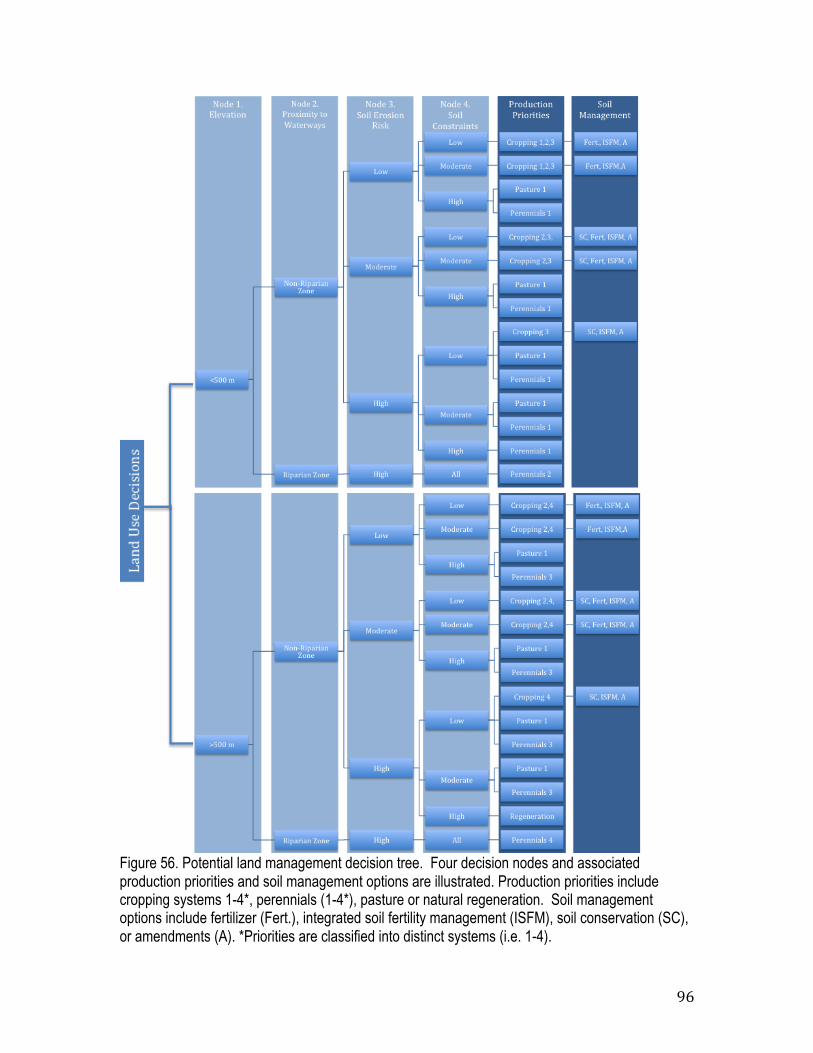
96
Figure 56. Potential land management decision tree. Four decision nodes and associated production priorities and soil management options are illustrated. Production priorities include cropping systems 1-4*, perennials (1-4*), pasture or natural regeneration. Soil management options include fertilizer (Fert.), integrated soil fertility management (ISFM), soil conservation (SC), or amendments (A). *Priorities are classified into distinct systems (i.e. 1-4).
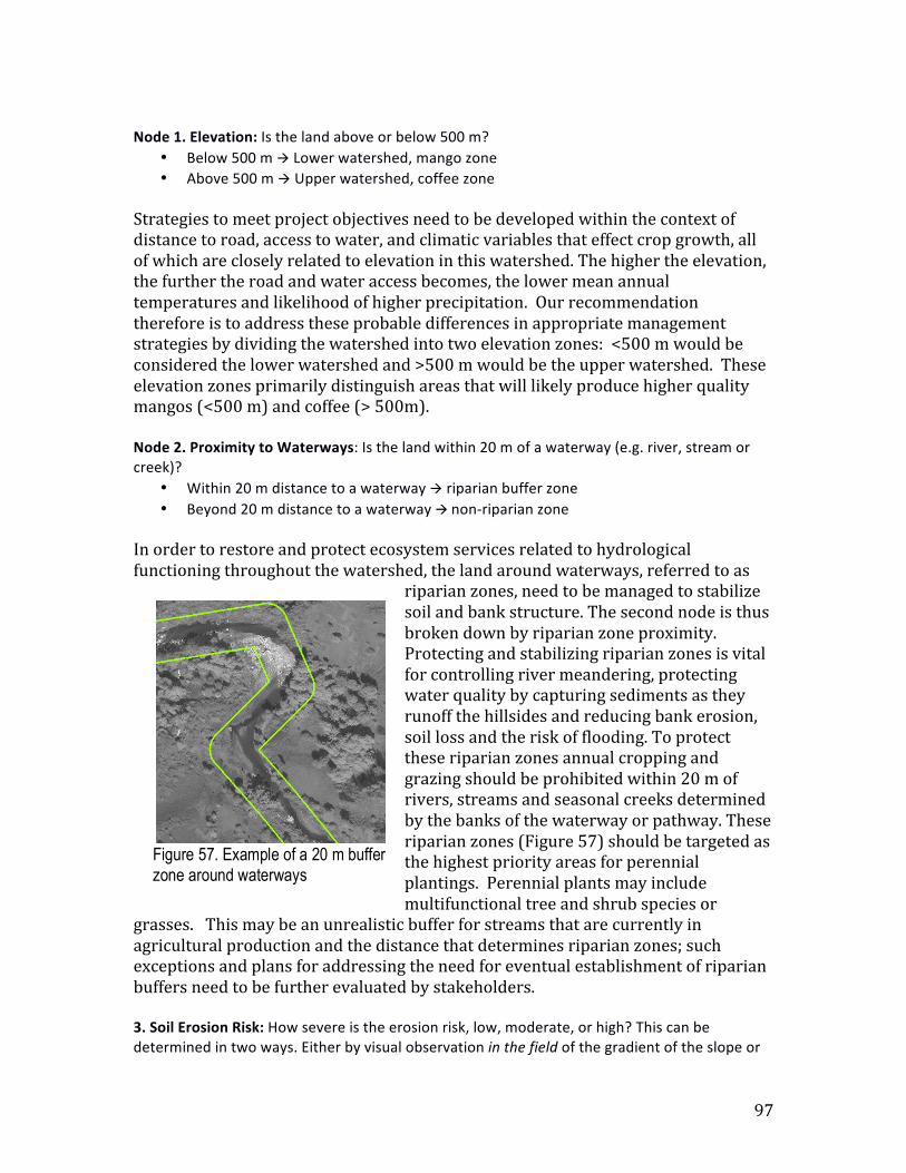
97
Node 1. Elevation: Is the land above or below 500 m?
• Below 500 m à Lower watershed, mango zone • Above 500 m à Upper watershed, coffee zone
Strategies to meet project objectives need to be developed within the context of distance to road, access to water, and climatic variables that effect crop growth, all of which are closely related to elevation in this watershed. The higher the elevation, the further the road and water access becomes, the lower mean annual temperatures and likelihood of higher precipitation. Our recommendation therefore is to address these probable differences in appropriate management strategies by dividing the watershed into two elevation zones: <500 m would be considered the lower watershed and >500 m would be the upper watershed. These elevation zones primarily distinguish areas that will likely produce higher quality mangos (<500 m) and coffee (> 500m). Node 2. Proximity to Waterways: Is the land within 20 m of a waterway (e.g. river, stream or creek)?
• Within 20 m distance to a waterway à riparian buffer zone • Beyond 20 m distance to a waterway à non-‐riparian zone
In order to restore and protect ecosystem services related to hydrological functioning throughout the watershed, the land around waterways, referred to as
riparian zones, need to be managed to stabilize soil and bank structure. The second node is thus broken down by riparian zone proximity. Protecting and stabilizing riparian zones is vital for controlling river meandering, protecting water quality by capturing sediments as they runoff the hillsides and reducing bank erosion, soil loss and the risk of flooding. To protect these riparian zones annual cropping and grazing should be prohibited within 20 m of rivers, streams and seasonal creeks determined by the banks of the waterway or pathway. These riparian zones (Figure 57) should be targeted as the highest priority areas for perennial plantings. Perennial plants may include multifunctional tree and shrub species or
grasses. This may be an unrealistic buffer for streams that are currently in agricultural production and the distance that determines riparian zones; such exceptions and plans for addressing the need for eventual establishment of riparian buffers need to be further evaluated by stakeholders. 3. Soil Erosion Risk: How severe is the erosion risk, low, moderate, or high? This can be determined in two ways. Either by visual observation in the field of the gradient of the slope or
Figure 57. Example of a 20 m buffer zone around waterways
98
using the Predicted Soil Erosion Risk map (Figure 54) which includes the gradient of the slope but also information about soil parameters that will determine more precisely the risk of soil erosion. In the field: Is the land on a level (0-‐16%), moderate (16-‐30%), or steep (>30%) slope?
• Level (0-‐16%) à soil erosion risk is Low • Moderate (16-‐30%) à soil erosion risk is Moderate. • Steep (>30%) à soil erosion risk is High.
Or Using the Predicted Soil Erosion Risk (PSER) map: Does the land have <50 Mg ha-‐1 yr-‐1, 50-‐100 Mg ha-‐1 yr-‐1 or > 100 Mg ha-‐1 yr-‐1) predicted soil erosion risk.
• <50 Mg ha-‐1 yr-‐1 à soil erosion risk is Low • 50 -‐ 100 Mg ha-‐1 yr-‐1 à soil erosion risk is Moderate. • > 100 Mg ha-‐1 yr-‐1 à soil erosion risk is High.
A key threat to the availability of a number of ecosystem services and a critical impediment to agricultural sustainability in this watershed is the excessive loss of soil from wind and water erosion. To reduce the soil erosion, specific cropping or soil conservation practices must be employed that are appropriately matched to the erosion risk. A visual determination of the gradient of the slope enables a farmer to generally determine how at-‐risk soils are for erosion without additional resources. The slope can also impact the efficiency of agricultural inputs such as mineral fertilizer. The likelihood that inputs such as fertilizer will be washed away before plants can utilize them increases with the gradient of the slope. While slope is an important factor for determining erosion, other factors such as the length of the slope, soil texture, and soil organic carbon concentration also play an important role but are not easily determined by visual inspection alone. Alternatively the severity of predicted soil erosion risk (PSER), calculated by the revised universal soil loss equations (RUSLE), is illustrated in the map in figure 54, can be used to determine the erosion risk of a particular site and the appropriate production and soil management options. Level slopes are zones where crop production is likely to have the highest potential yields, and risk of soil or input loss the lowest. In the lower watershed, level land is also a high priority for irrigation schemes, as water is most accessible, and construction of irrigation infrastructure is likely to result in the most cost effective returns. Level slopes in the upper watershed poses challenges to provide access to water and transport for any construction materials. As long as there are no soil restrictions (see Node 4 below) there are few management restrictions for these areas and these are likely areas where crop and soil appropriate fertilization strategies will have the highest impact on crops.

99
Soils on moderate slopes will likely result in more erosion and reduced efficiency of agricultural inputs. We therefore recommend for these sites that cropping system 2 or 4 be adopted in conjunction with soil conservation measures. To maximize the efficiency of agricultural inputs, soil and plant requirement information should be consulted (see below) particularly if there are any soil restrictions. Conservation practices such as contour planting of hedgerows or construction of swales are recommended for moderate and steep slopes. Steep slopes are the most vulnerable to erosion and should not be left bare at any time of the year. These lands should be targeted for perennial plantings of tree, shrubs or grasses and managed for fruit production, woodfuel, timber, or rotational grazing and soil conservation structures. Node 4. Soil constraints: Is the severity of soil constraints for plant productivity low, moderate or high? Again this can be determined in two ways, either by visual inspection in the field or preferably using a combination of digital maps and crop and tree requirement information. How severe are the visually obvious soil constraints either due to soil chemical properties such as pH or physical conditions such as soil depth?
• There are no obvious constraints à low • Plants on the site indicate nutrient deficiencies or other constraints related to soil
properties that may be ameliorated with the appropriate agricultural inputs. Plants have shown reduced germination and/or yield, discoloration, disease or severe weed invasion à moderate
• There are physical constraints that cannot be overcome with any agricultural inputs. The depth of the soil is < 20 cm (determined with a shovel or hoe), slope is >100% or there has been gully erosion à high
Or Using the soil map data how severe are soil constraints either due to soil chemical properties such as pH or physical conditions such as soil depth?
• There are few constraints (<6) determined by the Soil Constraint Indexà low • There are many constraints (>7) determined by the Soil Constraint Indexà moderate • There are physical constraints that cannot be overcome with any agricultural inputs.
The depth of the soil is < 20 cm, slope is >100% à high
Production Priority Options What are the most viable production priorities given the site’s elevation, proximity to waterway, soil erosion risk and soil constraints? Here we describe different production strategies for food, woodfuel, timber or other ecosystem services most appropriate for a given site’s conditions. We have grouped
100
these strategies into generalized cropping and perennial systems typical to the watershed to give a sense of what types of production strategies are appropriate. The list is not exhaustive but more illustrative as there are likely numerous strategies that farmers in the area have developed that would be effective. Cropping System 1 – Intensive annual: Low elevation sites, outside of riparian zones, with little soil erosion risk or soil constraints can be prioritized for annual crops, such as rice, maize or cassava that can be grown in high densities and with greater amounts of agricultural inputs including fertilizer and irrigation. These crops may be grown in monocultures but should be grown in rotations as locally recommended to avoid best build up. As soil erosion is a minor risk for this production system soil conservation practices are not a high priority. Although soil constraints are low and amendments such as compost and green manures are not required they are still highly recommended. Cropping System 2 – Intercropping annual: A wide range of sites both in the upper and lower watershed, in non-‐riparian zones, on soils with low to moderate risk of erosion and low to moderate soil constraints can be prioritized for intercropping of rain-‐fed annual crops. There are currently a number of intercropping combinations being practiced in the watershed that include some combinations of maize, beans, cassava, sweet potato, taro and yam. Intercropping is designed to reduce the risk of crop loss from disease or pests, and maximize soil resources. When this production strategy is practiced in areas with higher erosion risk, soil conservation practices should be employed. For areas with soil constraints, amendments such as compost and green manures are highly recommended. Fertilizers should be used with caution and in combination with organic inputs, particularly on moderate slopes. Digital maps of constraints should be consulted for application rates particularly the phosphorus sorption index (Figure 55) before fertilizers are applied. Cropping System 3 – Low elevation agroforestry: A wide range of sites in the lower watershed, in non-‐riparian zones, on soils with low to moderate risk of erosion and low to moderate soil constraints can be prioritized for intercropping of rain-‐fed or in some case irrigated semi-‐permanent crops, annual crops intercropped with semi-‐permanent or permanent crops (i.e. trees and shrubs). At these lower elevation sites semi-‐permanent crops may include cassava, plantain, fodder, and woodlots. Permanent crops include perennials such as mango, breadfruit, citrus, coconut, pigeon pea and avocado. Fruit and nut crops on soils with low erosion risk may be suitable for irrigation. For areas with soil constraints amendments such as compost and green manures are highly recommended. Fertilizers should be used with caution, particularly on moderate slopes, and applied specifically to certain crops or perennials in the system. Digital maps of constraints should be consulted for application rates particularly the phosphorus sorption index before fertilizers are applied.
101
Cropping System 4 – High elevation agroforestry: A wide range of sites in the upper watershed, in non-‐riparian zones, on soils with low to moderate risk of erosion and low to moderate soil constraints can be prioritized for intercropping of rain-‐fed or in some case irrigated semi-‐permanent crops, annual crops intercropped with semi-‐permanent or permanent crops (i.e. trees and shrubs). At these upper elevation sites semi-‐permanent crops may include cassava, pigeon pea, fodder, and woodlots. Permanent crops include perennials such as coffee, breadfruit, citrus, and avocado. Fruit and nut crops on soils with low erosion risk may be suitable for irrigation. For areas with soil constraints amendments such as compost and green manures are highly recommended. Fertilizers should be used with caution, particularly on moderate slopes. Digital maps of constraints should be consulted for application rates particularly the phosphorus sorption index (Figure 36) before fertilizers are applied. Pasture 1: On sites in the lower watershed non-‐riparian zones, on soils ranging from low to high erosion risk, with moderate to high constraints can be prioritized for pasture, improved and managed; rotational grazing is recommended for all slope levels. Perennials 1: On sites in the lower watershed non-‐riparian zones, on soils with erosion risk that is low to moderate but with high constraints or soils with high erosion risk can be prioritized for perennial production. It is critical that these sites be planted with trees or shrubs that are either coppicing or planned to be harvested on very long rotations (e.g. 20 years) to maintain soil and slope stability. Perennials 2: On sites in the lower watershed in riparian zones, soils are consider to have high erosion risk and should be prioritized for permanent perennial plantings. Perennials 3: On sites in the upper watershed non-‐riparian zones, on soils with erosion risk that is low to moderate but with high constraints or soils with high erosion risk can be prioritized for perennial production. It is critical that these sites be planted with trees or shrubs that are either coppicing or planned to be harvested on very long rotations (e.g. 20 years) to maintain soil and slope stability. Perennials 4: On sites in the upper watershed in riparian zones, soils are consider to have high erosion risk and should be prioritized for permanent perennial plantings. Regeneration: On sites where soil erosion risk and soil constraints are high agricultural production is likely to increase erosion and perennial plantings will likely require significant effort to maintain. We therefor recommend that these sites be left unmanaged and protected from grazing to allow for vegetation to regenerate naturally.
102
Soil Management Options What are the most appropriate soil management options for a recommended cropping system given the site’s elevation, proximity to waterway, soil erosion risk and soil constraints? Fertilizer (Fert) -‐ Sites in both the upper and lower watershed, with low to moderate soil erosion risk are suitable for fertilizer application. Fertilizer application rates range depend on the cropping system and slope (Table 9). Fertilizers should be used with caution and in combination with organic inputs, particularly on moderate slopes. Digital maps and tables of crop production constraints should be consulted to determine application rates particularly the phosphorus sorption index (Figure 38) before fertilizers are applied. Integrated Soil Fertility Management (ISFM) -‐ Sites in both the upper and lower watershed, with low to moderate soil erosion risk and low to moderate soil constraints or high soil erosion risk with low constraints are suitable for ISFM. ISFM includes a wide range of practices that enable the farmer better ensure nutrient use efficiency and improve soil quality. In general these practices are designed to increase soil organic matter and can be used in combination with targeted fertilizer or manure applications. ISFM practices include: growing and incorporating or mulching with green manures, usually nitrogen fixing species, either in rotation, intercropping or as hedgerows. Amendments (A) – It is recommended that sites throughout the watershed that have low to moderate soil constraints be targeted for soil amendments to help ameliorate constraints. Problems related to low pH, rare in the watershed, can be addressed through the application and incorporation of lime and compost. Soil Conservation (SC) – On sites with moderate to high soil erosion risk that are being used for agricultural production it is strongly recommended that soil conservation practices be used. Soil conservation practices may be vegetative including:
• Cover crops – Crops grown specifically to protect soil and/or build soil quality
• Ranpay – creole word for crop residue barriers (also known as trash lines) piled along the contour of the slope
• Hedgerows – perennial grasses, shrubs or trees planted along contour either within or at the edge of a field. Bann Manje, is a locally adapted hedgerow strategy that includes plants with economic value, such as pineapple.
Soil conservation practices may be constructed along contours of hillsides such as of swales, terraces or retaining walls.
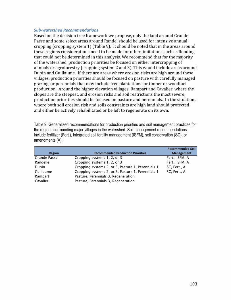
103
Sub-‐watershed Recommendations Based on the decision tree framework we propose, only the land around Grande Passe and some select areas around Randel should be used for intensive annual cropping (cropping system 1) (Table 9). It should be noted that in the areas around these regions considerations need to be made for other limitations such as flooding that could not be determined in this analysis. We recommend that for the majority of the watershed, production priorities be focused on either intercropping of annuals or agroforestry (cropping system 2 and 3). This would include areas around Dupin and Guillaume. If there are areas where erosion risks are high around these villages, production priorities should be focused on pasture with carefully managed grazing, or perennials that may include tree plantations for timber or woodfuel production. Around the higher elevation villages, Rampart and Cavalier, where the slopes are the steepest, and erosion risks and soil restrictions the most severe, production priorities should be focused on pasture and perennials. In the situations where both soil erosion risk and soils constraints are high land should protected and either be actively rehabilitated or be left to regenerate on its own.
Table 9: Generalized recommendations for production priorities and soil management practices for the regions surrounding major villages in the watershed. Soil management recommendations include fertilizer (Fert.), integrated soil fertility management (ISFM), soil conservation (SC), or amendments (A).
!"#$%& !"'%(("&)")*+,%)-'.$%&*+,$%,$.$"/!"'%(("&)")*0%$1*
23&3#"("&.Grande Passe Cropping systems 1, 2, or 3 Fert., ISFM, ARandelle Cropping systems 1, 2, or 3 Fert., ISFM, ADupin Cropping systems 2, or 3, Pasture 1, Perennials 1 SC, Fert., AGuillaume Cropping systems 2, or 3, Pasture 1, Perennials 1 SC, Fert., ARampart Pasture, Perennials 3, RegenerationCavalier Pasture, Perennials 3, Regeneration
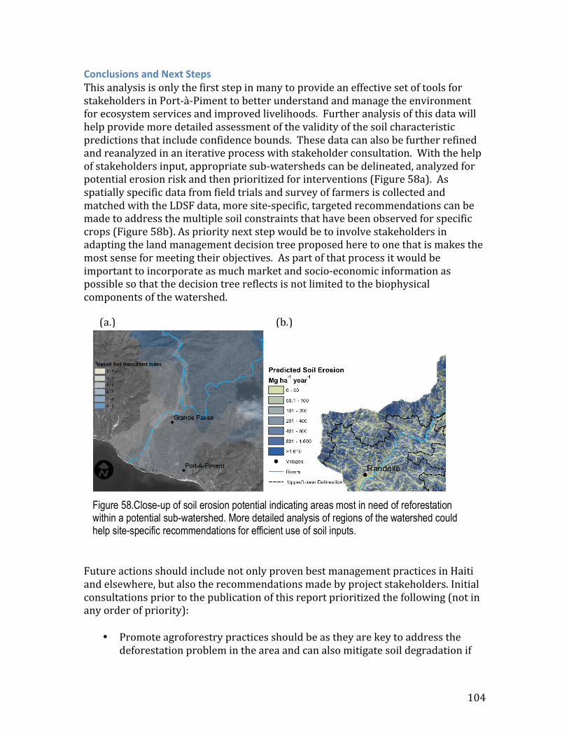
104
Conclusions and Next Steps This analysis is only the first step in many to provide an effective set of tools for stakeholders in Port-‐à-‐Piment to better understand and manage the environment for ecosystem services and improved livelihoods. Further analysis of this data will help provide more detailed assessment of the validity of the soil characteristic predictions that include confidence bounds. These data can also be further refined and reanalyzed in an iterative process with stakeholder consultation. With the help of stakeholders input, appropriate sub-‐watersheds can be delineated, analyzed for potential erosion risk and then prioritized for interventions (Figure 58a). As spatially specific data from field trials and survey of farmers is collected and matched with the LDSF data, more site-‐specific, targeted recommendations can be made to address the multiple soil constraints that have been observed for specific crops (Figure 58b). As priority next step would be to involve stakeholders in adapting the land management decision tree proposed here to one that is makes the most sense for meeting their objectives. As part of that process it would be important to incorporate as much market and socio-‐economic information as possible so that the decision tree reflects is not limited to the biophysical components of the watershed.
Future actions should include not only proven best management practices in Haiti and elsewhere, but also the recommendations made by project stakeholders. Initial consultations prior to the publication of this report prioritized the following (not in any order of priority):
• Promote agroforestry practices should be as they are key to address the deforestation problem in the area and can also mitigate soil degradation if
Figure 58.Close-up of soil erosion potential indicating areas most in need of reforestation within a potential sub-watershed. More detailed analysis of regions of the watershed could help site-specific recommendations for efficient use of soil inputs.
(a.) (b.)
105
managed properly. Top priority trees that have commercial values are coffee, citrus, pigeon pea, avocado.
• Establish woodlots on farm lands for charcoal production • Establish nurseries in key locations in the watershed to facilitate distribution
to farmers. The mountainous areas of Nan Gauvin and Cavalier were identified as priority locations.
• Launch a vast campaign of soil conservation at the watershed scale with different working incentive strategies (e.g. participatory, cash/food for work)
• Improved pasture management and animal husbandry was as a means to diversify income and reduce pressure on natural resources
Transitioning the steep slopes in the Port-‐à-‐Piment watershed from low yielding annual cropping to agroforestry production of higher value marketable crops such as mango or coffee needs to be planned carefully. While these perennial crops may provide higher economic returns and help stabilize eroding slopes, they will not do so for many years. As agroforestry systems mature farmers will need to continue to produce enough food and/or income to feed their families. Intercropping current cropping choices such as maize and beans with perennials such as mangos may be possible without dramatic yield reductions for much of this transition period. Site-‐specific fertility management, and planting densities need to be determined by cropping trials. Strategies to promote and incentivize the transition need to be developed. Incentive strategies could include direct payments based on the estimated value of ecosystem services that perennial production would provide; farmers could get payments for ecosystem services for the carbon stored in the newly planted tree and the reduced rate of erosion. At the same time marketing strategies for the higher value agroforestry products must be developed so that farmer will benefit from the transition as soon as the crops are productive.
106
Literature Cited This bibliography is available online at the Mendeley group site “Haitian Agriculture Forestry and Environment”: http://www.mendeley.com/groups/1854021/haitian-‐agriculture-‐forestry-‐and-‐environment/
CNIGS. 2002. Notes explicatives des cartes thématiques : Occupation du sol Risque réel d ’érosion. République D’Haïti Ministere de la Planification et de La Cooperation Externe.
Clermont-‐Dauphin, C., Y. Cabidoche, and J. Meynard. 2005. Diagnosis on the sustainability of an upland cropping system of southern Haiti. Agriculture Ecosystems and Environment 105:221-‐234. doi: 10.1016/j.agee.2004.03.008.
Van Diepen, C. A., H. van Keulen, J. Wolf, and J. A. A. Berkhout. 1991. Land evaluation: from intuition to quantification. Pages 139-‐ 204 in B. A. Stewart, editor. Advances in Soil Science, Volume 15. Springer-‐Verlag, New York.
FAO. 1976. A framework for land evaluation. FAO Soils Bulletin No. 32. Page 72. Rome, Italy.
FAO. 1993. Agroecological assessment for national planning: the example of Kenya. Bulletin 67. Rome, Italy.
Gumbs, F. A. 1997. Farmers and soil conservation in the Caribbean. UWICED Occasional Paper Series No. 3. Page 140. Kingston, Jamaica.
Hudson, N. W. 1977. Research needs for soil conservation in developing countries. In FAO. Soil conservation and management in developing countries. FAO Soils Bulletin No. 33. Pages 169-‐184. Rome, Italy.
Isaac, L., D. Shannon, and C. Wood. 2004. Hedgerow pruning management effects on maize yield and nitrogen uptake in an alley cropping system in Haiti. Agronomy Journal 96:1632-‐1640. Retrieved from http://links.isiglobalnet2.com/gateway/Gateway.cgi?GWVersion=2&SrcAuth=mekentosj&SrcApp=Papers&DestLinkType=FullRecord&DestApp=WOS&KeyUT=000225535800016.
Isaac, L., C. Wood, and D. Shannon. 2000. Decomposition and nitrogen release of prunings from hedgerow species assessed for alley cropping in Haiti. Agronomy Journal 92:501-‐511. Retrieved from http://links.isiglobalnet2.com/gateway/Gateway.cgi?GWVersion=2&SrcAuth=
107
mekentosj&SrcApp=Papers&DestLinkType=FullRecord&DestApp=WOS&KeyUT=000089408000016.
Klingebiel, A. A., and P. H. Montgomery. 1961. Land capability classification. Agriculture Handbook No. 210. Page 21. Washington, D.C.
Lim, K., Y. Park, and B. Engel. 2010. SATEEC GIS System for Spatiotemporal Analysis of Soil Erosion and Sediment Yield. intechopen.com 2003. Retrieved January 31, 2012, from http://www.intechopen.com/source/pdfs/23120/InTech-‐Sateec_gis_system_to_evaluate_soil_erosion_and_sediment_yield.pdf.
McBratney, a. 2003. On digital soil mapping. Pages 3-‐52 Geoderma. doi: 10.1016/S0016-‐7061(03)00223-‐4.
Mitasova, H., and W. M. Brown. 2012. Using Soil Erosion Modeling for Improved Conservation Planning: A GIS-‐based Tutorial. Retrieved from http://skagit.meas.ncsu.edu/~helena/gmslab/reports/CerlErosionTutorial/denix/denixstart.html.
NRCS. 2006. Revised Universal Soil Loss Equation, Version 2 (RUSLE2).
Nelson, M. a., T. F. a. Bishop, J. Triantafilis, and I. O. a. Odeh. 2011. An error budget for different sources of error in digital soil mapping. European Journal of Soil Science 62:417-‐430. doi: 10.1111/j.1365-‐2389.2011.01365.x.
R Development Core Team. 2008. R: A Language and Environment for Statistical Computing. Vienna.
Rahman, M. R., Z. H. Shi, and C. Chongfa. 2009. Soil erosion hazard evaluation—An integrated use of remote sensing, GIS and statistical approaches with biophysical parameters towards management strategies. Ecological Modelling 220:1724-‐1734. doi: 10.1016/j.ecolmodel.2009.04.004.
Sanchez, P. 2003. Fertility capability soil classification: a tool to help assess soil quality in the tropics. Geoderma 114:157-‐185. doi: 10.1016/S0016-‐7061(03)00040-‐5.
Sheng, T. C. 1971. A treatment-‐oriented land capability classification scheme for hilly marginal lands in the humid tropics. Paper prepared for the Latin American Watershed Management Seminar Argentina. Kingston, Jamaica.
Shepherd, K. D. 2011. Soil Properties Report -‐ Soil Chemical and Physical Reference Values Kisongo.
Small, C. 2004. The landsat ETM plus spectral mixing space. Remote Sensing of Environment 93:1-‐17. doi: 10.1016/j.rse.2004.06.007.
108
Smukler, S. M., S. M. Philpott, L. E. Jackson, A.-‐maria Klein, F. Declerck, L. Winowiecki, and C. A. Palm. 2012. Integrating Ecology and Poverty Reduction. Page (J. C. Ingram, F. DeClerck, and C. Rumbaitis del Rio, Eds.). Springer US, Boston, MA. doi: 10.1007/978-‐1-‐4419-‐0633-‐5.
Stenberg, B., R. A. Viscarra Rossel, A. M. Mouazen, and J. Wetterlind. 2010. Visible and near infrared spectroscopy in soil Science. Advances in Agronomy 107:163-‐215. Elsevier. Retrieved from http://linkinghub.elsevier.com/retrieve/pii/S0065211310070057.
Vågen, T.-‐G., K. D. Shepherd, M. G. Walsh, L. Winowiecki, L. T. Desta, and J. E. Tondoh. 2010. AfSIS Technical Specifications. Page Africa.
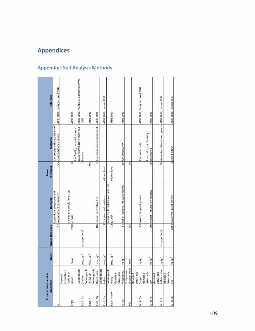
109
Appendices
Appendix I Soil Analysis Methods
!"#$%
!&&
'()*+('%+,
-./0$1,2'
3,4'()
*+('%+,-.
/0$1,2'
5'6'('"1'
!"
#$%
&'()*(+,-.)!/01!/02,1)'(+)
3*-20(,42*.(4)+.5*-*.(-*.1)
6$6
&'()-0(142'*()4/.)'7'*8'9*8*4:)05)
3014)(,42*.(4).8.3.(41
;5<=<)>?@@A)B2'+:)'(+)C
.*8)>??>
D&E<F
D8.-42*-'8)
&0(+,-4*7*4:)
E<0+*-*4:)02)
1'8*(*4:F
G<)-3
H@>???
1'8*(*4:)4/'4)I0,8+)8*3
*4)-20!)
J20I4/
?;5<=<)>?@@
DK-/$)&'
DK-/'(J.'98.)
&'8-*,3)
-308 -)LJH@
(0),!!.2)8.7.8
>
80I)5.24*8*4:)!04.(4*'8M)(023
'8)
-'8-*,3)!20304.1)/.'84/:)10*8)
9'-4.2*'
;5<=<)>?@@M);&=;N)>?@?A)B2'+:)'(+)C
.*8)
>??>
DK-/$)O
DK-/'(J.'98.)
P04'11*,3
-308 -)LJH@
?$6
;5<=<)>?@@
DK-/$)QJ
DK-/'(J.'98.)
Q'J(.1*,3
-308 -)LJH@
@??1'4,2'4.1).55.-4*7.)&D&
6L.:)-03!0(.(4)05)-/8020!/:88
;5<=<)>?@@
DK-/$)R'
DK-/'(J.'98.)
<0+*,3
-308 -)LJH@
@<0*8)142,-4,2'8)!2098.31
(0)80I.2)8.7.8
;5<=<)>?@@M)S'(+0()@TT@
DK-/$);-*+*4:
DK-/'(J.'98.)
;-*+*4:
-308 -)LJH@
?$6
'4)2*1L)502);8)40K*-*4:M)-'()8*3
*4)2004)
J20I4/
(0)80I.2)8.7.8
;5<=<)>?@@
QH%.)P
Q./8*-/H%)
DK42'-4'98.)
P/01!/02,1)
3J)LJH@)
6?
2*1L)05)8.'-/*(J)*(40)I'4.2)90+*.1
%?
80I)!20+,-4*7*4:
;5<=<)>?@@
P<=
P/01!/02,1)
<02!4*0()=(+.K
*(+.K
>6?
6?
QH%.)&,
Q./8*-/H%)
DK42'-4'98.)
&0!!.2
3J)LJH@)
>?
40K*-*4:)502)!8'(4)J20I4/
@80I)!20+,-4*7*4:
;5<=<)>?@@A)B2'+:)'(+)C
.*8)>??>
QH%.)U.
Q./8*-/H%)
DK42'-4'98.)
=20(
3J)LJH@)
>??*3
!'-4)P)'9102!4*0()-'!'-*4:
6?
D11.(4*'8)502)1:(4/.1*V*(J)
-/8020!/:88
;5<=<)>?@@
QH%.)<
Q./8*-/H%)
DK42'-4'98.)
<,85'4.H1,85,2)
3J)LJH@)
(0),!!.2)8.7.8
@?
14,(4.+)02)+.8':.+)-20!)J20I4/
;5<=<)>?@@M)S'(+0()@TT@
QH%.)W(
Q./8*-/H%)
DK42'-4'98.)
W*(-)
3J)LJH@)
@>?$T
40K*-*4:)502)!8'(4)J20I4/
X:*.8+)8*3
*4*(J
;5<=<)>?@@A)U'J.2*')>??T
7+8%#19-)9".
)1+'
2#19-)
&(,&
'($#'
%
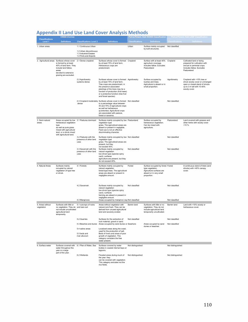
110
Appendix II Land Use Land Cover Analysis Methods
Classifications Level 1 Definitions Classifications Level 2 Definitions Classifications Definitions Classifications Definitions
1. Urban areas 1.1 Continuous Urban Urban Surface mainly occupied by built structures.
Not classified
1.2 Urban discontinuous1.3 Industrial Estates1.4 Ports and Airports
2. Agricultural areas Surfaces whose cover is formed by at least 40% of land farm. They include land fallow. areasdevoted to extensive grazing are excluded.
2.1 Dense cropland Surfaces whose cover is formed by at least 75% of land farm. Herbaceous crops are predominant.
Cropland Surface with at least 40% agriculture coverage. Includes fallow. Excludes Pastureland
Cropland Cultivated land or being prepared for cultivation with annual or perrenial crops. Includes fallow. Excludes Pastureland
2.2 Agroforestry systems dense
Surfaces whose cover is formed by at least 75% of land farm. Tree crops are predominant. in the presence associated plantings of the trees may be a function of production (fruit trees) or a protective function (tree fruit and forest species)
Agroforestry Surface occupied by bushes and trees. Agriculture is absent or in small proportion.
Agroforestry Cropland with >10% tree or shrub woody cover or unmanged open or closed stand of shrubs up to 3 m tall with 10-40% woody cover.
2.3 Cropland moderately dense
Surfaces whose cover is formed to a percentage value between 40 and 75% of agricultural crops as well as herbaceous qu'arborées. Agricultural crops are associated with pasture, forest or savanna.
Not classified Not classified
3. Semi-natural areas
Areas occupied by low herbaceous vegetation typeas well as pure grass mixed with agricultural land, or a shrub mixed with agricultural land.
3.1 Pastures dominant Surfaces mainly occupied by low vegetation typegrass. The agricultural areas are absent or present in negligible. Feed use is not an effectivediscriminating character.
Pastureland Surface occupied by herbaceous vegetation. Can be mixed with agriculture.
Pastureland Land covered with grasses and other herbs with woody cover <10 %.
3.2 Pastures with the presence of other land uses
Surfaces mainly occupied by low vegetation typegrass. The agricultural areas are present, but theynot exceed 40%.
Not classified Not classified
3.3 Savannah with the presence of other land uses
Surfaces mainly occupied by natural vegetationlow shrub type (species spiny cacti). surfacesagriculture are present, but they do not exceed 40%.
Not classified Not classified
4. Natural Areas Surfaces mainly occupied by natural vegetation of type tree or shrub.
4.1 Forests Surfaces mainly occupied by natural vegetationforest-type trees. The agricultural areas are absent or present in negligible amount.
Forest Surface occupied by forest type vegetation. Agriculture surfaces are absent or in very small proportion.
Forest A continuous stand of trees (and shrubs) with >40% canopy cover.
4.2 Savannah Surfaces mainly occupied by natural vegetationlow shrub type (species spiny cacti). surfacesfarming are absent or present in negligible amount.
Not classified Not classified
4.3 Mangroves Areas occupied by mangrove vegetation.Not classified Not classified
5. Areas without vegetation
Surfaces with little or no vegetation. They do not include uncultivated agricultural land temporarily.
5.1 outcrops of rocks and bare soil
Areas without vegetation with natural rock flush. They can be derived from unused agricultural land and severely eroded.
Barren land Surfaces with little or no vegetation. They do not include agricultural land temporarily uncultivated.
Barren land Land with <10% woody or herbaceous cover.
5.2 Quarries Surfaces for the extraction of rock material, gravel or sand.
Not classified Not classified
5.3 Beaches and dunes Areas occupied by sand dunes or beaches.Seashore Areas occupied by sand dunes or beaches.
Not classified
5.4 saline areas Localized areas along the coast, used for the production of salt.
5.5 beds and river alluvium
Beds of rivers and areas of poor growth of vegetation. This category considers the free water present.
6. Surface water Surfaces covered with water throughout the year or a largepart of the year.
6.1 Plan of Water, Sea Surfaces covered by water bodies in coastal internal bays or lagoons.
Not distinguished Not distinguished
6.2 Wetlands Flooded areas during much of the year. theycan be covered with vegetation. This category excludes not the rice fields.
Not distinguished Not distinguished
CNIGS (Corine) Port-à-Piment, Haiti IKONS Classification Port-à-Piment, Haiti LDSF Classification