Belgium | Austria | Bulgaria | Cyprus | Czech Republic | Finland | Germany | Greece | Ireland | Latvia | Lithuania | Luxembourg | Malta | Netherlands | Poland | Portugal | Slovakia | Spain | Sweden|

baseline.vias.be

Methodological guidelines – KPI Post-crash Care

Version 2.1, April 28, 2021

2/18

Belgium | Austria | Bulgaria | Cyprus | Czech Republic | Finland | Germany | Greece | Ireland | Latvia | Lithuania | Luxembourg | Malta | Netherlands | Poland | Portugal | Slovakia | Spain | Sweden|

baseline.vias.be

Project: This document has been prepared in the framework of the BASELINE project, for which a grant has been awarded by the European Commission. Information on this project can be found on the website www.baseline.vias.be

References: (1) Grant agreement under the Connecting Europe Facility (CEF) No MOVE/C2/SUB/2019-558/CEF/PSA/SI2.835753 collection of Key Performance Indicators (KPIs) for road safety (2) Consortium agreement among the 19 partners of the Baseline project

Authors: Wouter Van den Berghe, Vias institute (Belgium), Nina Nuyttens, Vias institute (Belgium), Maria Segui Gomez, consultant (Spain), Frits Bijleveld, SWOV (the Netherlands) and Wendy Weijer-mars, SWOV (the Netherlands)

Publisher: Vias institute, Brussels, Belgium (www.vias.be)

Please refer to this document as follows: “Van den Berghe, W. et al. (2021). Methodological guidelines – KPI Post-crash Care. Baseline pro-ject, Brussels: Vias institute”

Any comments or feedback regarding these guidelines, should be sent to baseline@vias.be.

Version history

Version Date Changes

1.0 15 – 02 – 2021 First draft - not yet discussed in the KPI expert group for Post crash care

2.0 15 – 03 – 2021 Second draft, based on feedback of KPI expert group

2.1 28 - 04 - 2021 Minor adjustments + addition of Annex on sampling

3/18

Contents

Version history .................................................................................................................................... 2

Contents .............................................................................................................................................. 3

Terminology ........................................................................................................................................ 4

1 Introduction ................................................................................................................................. 5

2 Data required for the calculation of the KPI on post-crash care ............................................. 5

2.1 Data sources ________________________________________________________________ 5

2.2 Need for clear definition and scope ______________________________________________ 6

2.3 Data access _________________________________________________________________ 6

2.4 Possible data quality issues ____________________________________________________ 6

3 KPI values to be provided ........................................................................................................... 7

3.1 Minimum requirements _______________________________________________________ 7

3.1.1 Value ................................................................................................................................................. 7

3.1.2 Year ................................................................................................................................................... 7

3.1.3 Breakdowns by road type or type of area ........................................................................................ 7

3.2 Possibilities for additional information and breakdowns _____________________________ 7

3.2.1 Data ................................................................................................................................................... 7

3.2.2 Further breakdowns ......................................................................................................................... 8

3.2.3 Additional percentiles ....................................................................................................................... 8

3.2.4 Rearrangement of the data .............................................................................................................. 8

3.2.5 Additional years ................................................................................................................................ 8

3.2.6 Possibilities for alternative indicators .............................................................................................. 9

3.2.7 Useful contextual information ......................................................................................................... 9

4 Sampling methodology .............................................................................................................. 9

4.1 Population __________________________________________________________________ 9

4.2 Minimum total sample size_____________________________________________________ 9

4.3 Stratification _______________________________________________________________ 10

4.4 Sampling of EMS stations and further sampling ___________________________________ 10

4.5 Post-stratification weights and statistical analysis _________________________________ 10

5 Expected results ......................................................................................................................... 11

6 References .................................................................................................................................. 11

Annex. Extracts from the SWD document in relation to post-crash care .................................... 12

4/18

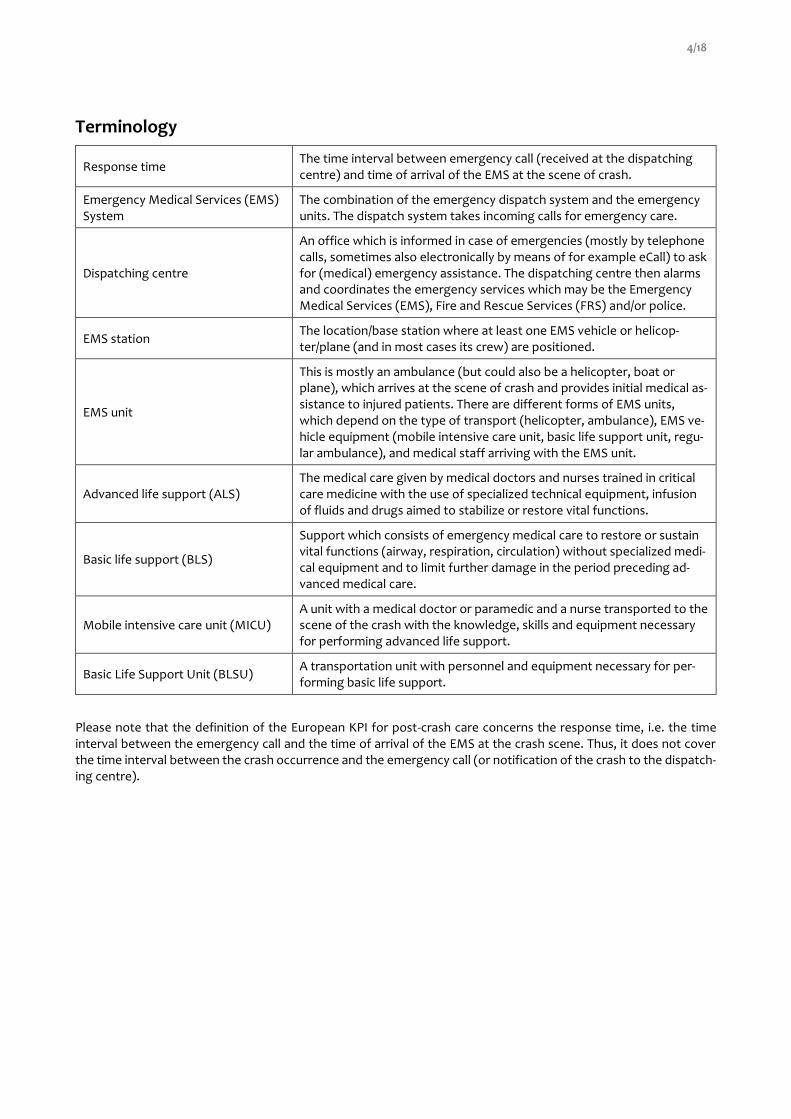
Terminology

Response time The time interval between emergency call (received at the dispatching centre) and time of arrival of the EMS at the scene of crash.

Emergency Medical Services (EMS) System

The combination of the emergency dispatch system and the emergency units. The dispatch system takes incoming calls for emergency care.

Dispatching centre

An office which is informed in case of emergencies (mostly by telephone calls, sometimes also electronically by means of for example eCall) to ask for (medical) emergency assistance. The dispatching centre then alarms and coordinates the emergency services which may be the Emergency Medical Services (EMS), Fire and Rescue Services (FRS) and/or police.

EMS station The location/base station where at least one EMS vehicle or helicop-ter/plane (and in most cases its crew) are positioned.

EMS unit

This is mostly an ambulance (but could also be a helicopter, boat or plane), which arrives at the scene of crash and provides initial medical as-sistance to injured patients. There are different forms of EMS units, which depend on the type of transport (helicopter, ambulance), EMS ve-hicle equipment (mobile intensive care unit, basic life support unit, regu-lar ambulance), and medical staff arriving with the EMS unit.

Advanced life support (ALS) The medical care given by medical doctors and nurses trained in critical care medicine with the use of specialized technical equipment, infusion of fluids and drugs aimed to stabilize or restore vital functions.

Basic life support (BLS)

Support which consists of emergency medical care to restore or sustain vital functions (airway, respiration, circulation) without specialized medi-cal equipment and to limit further damage in the period preceding ad-vanced medical care.

Mobile intensive care unit (MICU) A unit with a medical doctor or paramedic and a nurse transported to the scene of the crash with the knowledge, skills and equipment necessary for performing advanced life support.

Basic Life Support Unit (BLSU) A transportation unit with personnel and equipment necessary for per-forming basic life support.

Please note that the definition of the European KPI for post-crash care concerns the response time, i.e. the time interval between the emergency call and the time of arrival of the EMS at the crash scene. Thus, it does not cover the time interval between the crash occurrence and the emergency call (or notification of the crash to the dispatch-ing centre).

5/18

1 Introduction

The Communication of the European Commission “Europe on the Move – Sustainable Mobility for Europe: safe, connected and clean” of the 13th May 2018 confirmed the EU's long-term goal of moving close to zero fatalities in road transport by 2050 and added that the same should be achieved for serious injuries. It also proposed new in-terim targets of reducing the number of road deaths by 50% between 2020 and 2030 as well as reducing the number of serious injuries by 50% in the same period. To measure progress, the most basic – and important – indicators are of course the result indicators on deaths and serious injuries.

In order to gain a much clearer understanding of the different issues that influence overall safety performance, the Commission has elaborated, in cooperation with Member State experts, a first set of key performance indicators (KPIs). The KPIs relate to the main road safety challenges to be tackled, namely: (1) infrastructure safety, (2) vehicle safety, (3) safe road use including speed, alcohol, distraction and the use of protective equipment, and (4) emer-gency response. The aim of the KPIs is connected to EC target outcomes.

The aim of the BASELINE project, funded partially by the European Commission, is to assist participating Member States’ authorities in the collection and harmonized reporting of these KPIs and to contribute to building the ca-pacity of Member States which have not yet collected and calculated the relevant data for the KPIs. The outcomes of this project will be used to set future European targets and goals based on the KPIs.

The purpose of this document is to further describe the minimal methodological requirements to qualify for the BASELINE KPI for post-crash care, defined as

The time elapsed in minutes and seconds between the emergency call following a road crash resulting in personal injury and the arrival at the scene of the road crash of the emergency services (to the value of the 95th percentile).

The minimal requirements set by the EC for this KPI are described in the Commission Staff Working Document SWD (2019) 283.

One possible data collection method is to draw a representative sample of responses to emergency calls in relation to road traffic crashes and base the analyses on this sample. If feasible, an even better approach is to consult a national administrative database for emergency calls and to select all calls related to road traffic crashes. This would allow the KPI to be calculated on the total population of emergency calls, without the need for weighting or extrap-olation. It is recommended that sampling should only be used if no national database can be used for calculating the KPI.

The following section describes the nature of the data required, regardless of which data collection method is used.

2 Data required for the calculation of the KPI on post-crash care

2.1 Data sources

In order to calculate the KPI on post-crash care, it is necessary to identify the time of the emergency call and the time of arrival of the emergency service. An intervention typically consists of several steps performed by emergency teams (Nemeckova & Atchison, 2019):

(1) receipt of the call (2) dispatching of the call (3) travelling to the crash scene (4) arrival and care at the crash scene (5) patient transfer to a medical facility.

For the calculation of the KPI we need the time stamps corresponding with step (1) and step (4). Whether that data – disaggregated or aggregated – is easy to retrieve depends on how the EMS system is organized in a particular country and how EMS data is collected, stored and aggregated. The most convenient situation is where a country has a dataset in which both timestamps are registered. In that case it is not necessary to link / combine datasets to calculate response rates.

6/18

However, this is not the case in all countries. Information about the timestamps may be scattered across different datasets and different data owners, such as: the Ministry of Public Health, individual hospitals, ambulance services, the police, individual dispatch centres, Ministry of Internal Affairs, a dedicated agency, regional public authorities or other stakeholders. Countries that are in this situation should ideally ensure a link between the respective datasets, but this will not always be possible due to the lack of common IDs and overlapping information in the datasets.

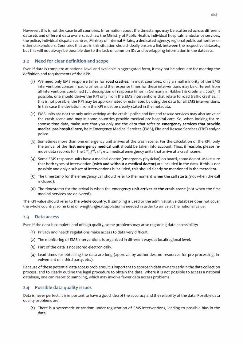
2.2 Need for clear definition and scope

Even if data is complete at national level and available in aggregated form, it may not be adequate for meeting the definition and requirements of the KPI:

(1) We need only EMS response times for road crashes. In most countries, only a small minority of the EMS interventions concern road crashes, and the response times for these interventions may be different from all interventions combined (cf. description of response times in Germany in Hakkert & Gitelman, 2007). If possible, one should derive the KPI only from the EMS interventions that relate to road traffic crashes. If this is not possible, the KPI may be approximated or estimated by using the data for all EMS interventions. In this case the deviation from the KPI must be clearly stated in the metadata.

(2) EMS units are not the only units arriving at the crash: police and fire and rescue services may also arrive at the crash scene and may in some countries provide medical pre-hospital care. So, when looking for re-sponse time data, make sure that you only use the data that refer to emergency services that provide medical pre-hospital care, be it Emergency Medical Services (EMS), Fire and Rescue Services (FRS) and/or police.

(3) Sometimes more than one emergency unit arrives at the crash scene. For the calculation of the KPI, only the arrival of the first emergency medical unit should be taken into account. Thus, if feasible, please re-move data records for the 2nd, 3rd, 4th, etc. medical emergency units that arrive at a crash scene.

(4) Some EMS response units have a medical doctor (emergency physician) on board, some do not. Make sure that both types of intervention (with and without a medical doctor) are included in the data. If this is not possible and only a subset of interventions is included, this should clearly be mentioned in the metadata.

(5) The timestamp for the emergency call should refer to the moment when the call starts (not when the call is closed).

(6) The timestamp for the arrival is when the emergency unit arrives at the crash scene (not when the first medical services are delivered).

The KPI value should refer to the whole country. If sampling is used or the administrative database does not cover the whole country, some kind of weighting/extrapolation is needed in order to arrive at the national value.

2.3 Data access

Even if the data is complete and of high quality, some problems may arise regarding data accessibility:

(1) Privacy and health regulations make access to data very difficult.

(2) The monitoring of EMS interventions is organized in different ways at local/regional level.

(3) Part of the data is not stored electronically.

(4) Lead times for obtaining the data are long (approval by authorities, no resources for pre-processing, in-volvement of a third party, etc.).

Because of these potential data access problems, it is important to approach data owners early in the data collection process, and to clearly outline the legal procedure to obtain the data. Where it is not possible to access a national database, one can resort to sampling, which may involve fewer data access problems.

2.4 Possible data quality issues

Data is never perfect. It is important to have a good idea of the accuracy and the reliability of the data. Possible data quality problems are:

(1) There is a systematic or random under-registration of EMS interventions, leading to possible bias in the data.

7/18

(2) The database includes erroneous data, errors or many outliers, which requires a tedious cleaning process before the data can be used for calculating the KPI. The metadata should clearly state the proportion of interventions for which the response times are unknown/ erroneous.

If the initial KPI value has an incorrect scope and/or does not meet all the methodological criteria, it is recommended to provide a recalculated or estimated value. In such cases the original KPI value before recalculation must also be provided and the estimation method must be documented in the metadata.

3 KPI values to be provided

3.1 Minimum requirements

3.1.1 Value

The minimum requirement is to provide the 95th percentile of the time elapsed between the emergency call and the arrival of the emergency services at the crash scene. The unit of measurement is minutes and seconds.

Where sampling is used, it is also required to provide a 95% confidence interval for this 95th percentile value. Since this calculation is not straightforward, Annex 2 provides further explanation on how to do this.

3.1.2 Year

The value should refer to a whole year. This should be the most recent value available. Because 2020 is an excep-tional and anomalous year due to the COVID crisis, it is requested to provide the KPI for 2019 if possible (or an earlier year of the data if 2019 is not yet available).

3.1.3 Breakdowns by road type or type of area

If available, the Commission proposes to make a breakdown by road type. Three types of roads are foreseen:

• urban roads (roads in built-up areas)

• non-urban roads (excluding motorways/highways)

• motorways/highways.

It is recognized that the distinction between urban roads and non-urban roads differs between countries (and some-times also between regions within a country). Therefore, the Baseline partners should explain which criteria were used to differentiate between types of roads. Moreover, they should ensure that the road categorisations are used in a consistent way across the different KPIs (in most other KPIs, road type is a compulsory variable).

Alternatively, if such a categorization is available, a breakdown of the KPI value can be provided which distinguishes between areas by population density. Possible categorisations could be based on

(a) the degree of urbanization used by EUROSTAT - cities, towns & suburbs, rural areas, or

(b) the rural-urban typology that is used by EUROSTAT for NUTS level 3 regions in the EU: predominantly rural regions, intermediate regions and predominantly urban regions.

3.2 Possibilities for additional information and breakdowns

Although none of the possibilities that are listed under this heading are mandatory, Member States are invited to consider providing one or more of those values (in addition to the formal, country level KPI value), in particular if such data is easily available.

3.2.1 Data

Ideally, the cleaned dataset (at record level) should be provided alongside the KPI value. This would be a table with a record for each intervention, including an ID, two or more timestamps and some other variables that can be used for making breakdowns and weighting the individual values.

The Member State should indicate by which method (including, where appropriate, weighting and extrapolation) the 95th percentile has been calculated. The data table should allow an independent researcher to calculate the KPI and compare with the value proposed by the Member State.

8/18

If for privacy reasons or other legal restrictions such record-level data cannot be provided, the Member State should provide aggregated values at the highest level of disaggregation possible.

3.2.2 Further breakdowns

If available, it is suggested to also provide (data for) the following breakdowns (for 2019 only):

• Location of crash (1) Area type: cities, towns & suburbs, rural areas – or predominantly urban, intermediate, predomi-

nantly rural (2) NUTS3 region of the location of the crash (3) Municipality (4) Exact crash location (if available and transferable)

• Time of arrival (1) Month (2) Day of week (3) Hour (or at least day/night) (4) Exact date and hour

• E-call warning: was the dispatching centre notified of the crash via e-call (Yes/No)

• Crash severity (1) Number of casualties in the crash (incl. fatalities) (2) Number of fatalities in the crash on arrival at the location of the crash (3) Number of fatalities in the crash on arrival at the hospital

• Type of emergency services (1) Medical Emergency Services, Fire and Rescue Services, or both (2) EMS vehicle equipment (mobile intensive care unit, basic life support unit, regular ambulance) (3) Presence of emergency physician at crash: yes/no

• Transport mode

• Crash with or without motorized vehicles involved

3.2.3 Additional percentiles

For analysis, research and benchmarking purposes it can be useful to also calculate some other percentile values:

• 25th percentile (1st quartile)

• 50th percentile (median)

• 75th percentile (3rd quartile)

• 85th percentile

• 99th percentile. The calculation of this value should be relatively straightforward if a good database is available from which the 95th percentile has already been calculated, since the methods for calculating the additional percentiles are identical as the method for calculating the 95th percentile.

3.2.4 Rearrangement of the data

An additional or alternative way for presenting the data is to calculate which percentage of the EMS interventions arrives at the crash scene within the following time intervals:

• 10 minutes

• 12 minutes

• 15 minutes

• 20 minutes

Please note that current good practice is that 95% of the EMS units are at the crash scene in less than 15 minutes after the emergency call (Hafen et. al, 2006).

3.2.5 Additional years

If there is a historic database of good quality, based on consistent definitions and registrations, it is suggested to provide KPI data starting from 2010 onwards (for the 95th percentile value). Such data could be useful for further analysis and benchmarking and could be used to estimate a value for 2019 if not available.

9/18

3.2.6 Possibilities for alternative indicators

Alternative, optional indicators, suggested at UN level, are

• % of serious injury crashes where no emergency care services were provided

• % of road traffic crashes resulting in serious injury where the response time did not exceed the national target

If such information is available, it can be added to the Baseline database. However, these values should not be used as a substitute but rather as a complement for the official European KPIs.

The definition of serious injury varies across countries. When providing values for these indicators, information should be added on what definitions have been used for defining serious injuries. If available, it is recommended to use the MAIS3+ definition.

3.2.7 Useful contextual information

For a correct interpretation of response times, for benchmarking with other countries, and for the selection of ap-propriate countermeasures, it is useful to provide the following contextual information:

• number of dispatching centres

• number of EMS transportation units

• number of EMS stations

• annual number of emergency calls

• annual number of emergency calls related to road crashes

• % of emergency calls relating to road crashes within the total number of emergency calls.

The following information on data quality is also useful contextual information:

• % of interventions for which the timestamp ‘emergency call’ is unknown

• % of interventions for which the timestamp ‘arrival at the scene of the road crash’ is unknown

• % of interventions for which both the timestamps ‘emergency call’ and ‘arrival at the scene of the road crash’ are unknown.

4 Sampling methodology

The previous sections covered both the use of a national administrative database and sampling of EMS interven-tions. For many countries it is expected that it is possible to get data from a national administrative database for emergency calls. Consequently, sampling will not be needed and the KPI could be calculated based on the total population of emergency calls. It is recommended to use sampling only if no national database can be used for calculating the KPI. Countries that use a national database for the estimation of the KPI can skip Chapter 4.

4.1 Population

The theoretical population refers to the national total of response times between the emergency calls following a crash resulting in personal injury and the arrival of the emergency services at the scene of the crash. EMS units are not the only units arriving at the crash. Police and fire and rescue services may also arrive at the crash scene and may in some countries provide medical pre-hospital care. So, when considering response time data, one should make sure to only use the data that refer to emergency services that provide medical pre-hospital care, be it Emer-gency Medical Services (EMS), Fire and Rescue Services (FRS) and/or police. Emergency services that provide both Advanced Life Support and Basic life Support should be included.

4.2 Minimum total sample size

In line with the sampling approach proposed for other KPIs, the minimum total sample size should be 2000. For some small countries, it may not be feasible to achieve this sample size, e.g. due to a relatively low number of road crashes involving injuries and/or a low number of interventions. In that case, a smaller sample size is acceptable.

It is likely that the distribution of response times in a country will not perfectly follow a normal distribution. It is expected that the distribution of response times will be right-skewed, with a larger spread of observations in the

10/18

second half of (longer) response times than in the first half of response times. Therefore, it is difficult to estimate in advance how large the confidence intervals of the 95th percentile will be1.

Accuracy for specific strata/subgroups, e.g. breakdowns for road types or types or areas, will by definition be lower. If higher accuracy levels are required for particular strata/subgroups (e.g. according to region of the country), it will be necessary to increase the sample size.

4.3 Stratification

In order to ensure a nationally representative sample, it is recommended to stratify according to regions, e.g. the areas at NUTS1 level.

Since the overall estimate is expected to be representative for the whole country, the theoretically optimal strategy is to sample all strata according to their proportion in the national number of (interventions related to) road crashes resulting in personal injuries. This strategy would, however, be detrimental for the accuracy of estimates for regions with a low number of interventions/traffic crashes. Hence, oversampling for such regions is allowed. By comparing the proportion of interventions by region in the sample with the proportion of interventions by region in the total population (or with the proportion of injury crashes in official statistics if the information on interventions is not available) selection probabilities and weights can be derived.

4.4 Sampling of EMS stations and further sampling

Within each region, either all EMS stations or a random sample of the EMS stations need to be selected. In the case of a sample, it is suggested

• to use results from at least 10 different EMS stations within each region (if possible)

• to ensure that at least 5% of the total number of EMS stations is represented, and

• to guarantee that the minimum total sample size of 2000 interventions is achieved.

The purpose of the random selection of EMS stations is to obtain a representative sample and to neutralise the effect of variables that may influence the KPI estimate, such as the road type and the area type in which the EMS station is mainly active and the type of emergency services that is provided by the EMS station. However, further stratification based on these and other variables is also allowed within the region strata.

As a further sub-selection of interventions in EMS stations may be an unusual task for those responsible for the data and may be labour-intensive and cause bias in the data selected, it is recommended to select all interventions from all selected EMS stations. If this is not possible, it is recommended to perform another simple random sampling of at least 5% of all interventions in this second sampling phase.

The Commission suggests a breakdown of the KPI by road type. Regardless of whether the sample is stratified by this variable or not, the three road types should be well defined in the methodology, including how they are deter-mined (e.g. typical characteristics, traffic signs, speed regimes, number of lanes…). They should be defined in the same way as the other European KPIs (in most of them a breakdown by road type is required).

It should be specified if the sample is biased in some way (area type, emergency type, time (all months, day of the week, and hour to be represented)).

4.5 Post-stratification weights and statistical analysis

To calculate the final KPI, the following procedure should be applied:

(1) Weight the observations (actual times recorded) with an appropriate weighting factor, taking into account all combinations of strata. It is recommended to use the exact values for each combination of stratification levels considered (e.g. emergency calls on motorways in region X). If these combined data are not available, the second-best option is to assume independence of all levels of stratification and use combinations of mar-ginal totals to estimate specific combinations.

(2) Calculate the 95th percentile for the total weighted sample and for the weighted breakdowns separately. (3) Calculate confidence intervals (for instance by using bootstrap techniques2).

1 In Annex 2, a method and formula is provided to calculate this confidence interval. 2 Guidance on applying bootstrap techniques is provided in Annex 2.

11/18

Results should then not only include the unweighted number of cases the overall result is based on, but also the number of bootstrap samples it is based on, or in general, information on how the interval is determined.

5 Expected results

The main KPI is the 95th percentile of response times between the emergency calls following a road crash resulting in personal injury and the arrival of the emergency services at the scene of the crash.

As a minimum, the 95th percentile for the whole country should be provided for 2019 (or an earlier year if data for 2019 is not yet available), and if possible a breakdown by road type or area type.

If feasible it is recommended to also provide the breakdowns mentioned in section 3.2.2 and the additional data and information mentioned in section 3.2. Together with the above estimates, a note or short report should be submit-ted that describes the specificities of the methodology.

If case sampling is used, a 95% confidence interval is expected. Results should include the unweighted number of interventions the result is based on (and the unweighted number per stratum), and the statistical techniques used to weight and analyse the results.

6 References

European Commission (2019). Commission staff working document EU road Safety Policy Framework 2021-2030 - Next steps towards "Vision Zero". SWD(2019) 283 final. Retrieved from https://ec.eu-ropa.eu/transport/sites/transport/files/legislation/swd20190283-roadsafety-vision-zero.pdf

Hafen, K., Lerner, M., Allenbach, R., Verbeke, T., Eksler, V., & Haddak, M. … Rackliff L. (2006). State of the art Re-port on Road Safety Performance Indicators. Deliverable D3.1 of the EU FP6 project SafetyNet. Retrieved from http://www.dacota-project.eu/Links/erso/safetynet/fixed/WP3/Delivera-ble%20wp%203.1%20state%20of%20the%20art.pdf

Hakkert, A.S. and V. Gitelman (Eds.) (2007) Road Safety Performance Indicators: Manual. Deliverable D3.8 of the EU FP6 project SafetyNet. Retrieved from http://www.dacota-project.eu/Links/erso/safe-tynet/fixed/WP3/sn_wp3_d3p8_spi_manual.pdf

Nemeckova, M. and Atchison L. (2019). An overview of post-collision response and emergency care in the EU. Brus-sels: European Transport Safety Council. Retrieved from https://etsc.eu/wp-content/uploads/Revive_Re-port.pdf

Van den Berghe, W., Fleiter, J.J. & Cliff, D. (2020) Towards the 12 voluntary global targets for road safety. Guidance for countries on activities and measures to achieve the voluntary global road safety performance targets. Brussels: Vias institute and Genève: Global Road Safety Partnership. Retrieved from https://www.grsproad-safety.org/wp-content/uploads/Towards-the-12-Voluntary-Global-Targets-for-Road-Safety.pdf

12/18

Annex 1. Extracts from the SWD document in relation to post-crash care

Reference: COMMISSION STAFF WORKING DOCUMENT - EU Road Safety Policy Framework 2021-2030 - Next steps towards "Vision Zero, SWD (2019) 238, https://ec.europa.eu/transport/sites/transport/files/legislation/swd20190283-roadsafety-vision-zero.pdf

Fast and effective emergency response

About 50% of deaths from road traffic collisions occur within minutes at the scene or in transit and before arrival at hospital. For those patients who are taken to hospital, 15% of deaths occur within the first 4 hours after the crash, and 35% occur after 4 hours3. Post-crash (trauma) care or trauma management refers to the initial medical treatment provided after a crash, whether it is administered at the scene, during the transportation to a medical centre or indeed subsequently. Effective post-crash care, including fast transport to the correct facility by qualified person-nel, reduces the consequences of injury. Research indicates that reducing the time between the crash and the arrival of emergency medical services from 25 to 15 minutes could reduce deaths by one third4 and that systematised train-ing of rescue and ambulance teams may reduce the extrication time of entrapped car and truck crash victims by 40-50%.

In this context, the Commission is closely monitoring the effects of the roll-out of eCall5, the automated emergency call in the event of a crash.

A regards post-crash care, the Commission

- is assessing the effect of eCall and will be evaluating the possible extension to other categories of ve-hicles (heavy goods vehicles, buses and coaches, motorcycles, and agricultural tractors);

- is facilitating closer contacts between road safety authorities and the health sector to assess further practical and research needs (e.g. how to improve on-scene diagnosis as well as communication sys-tems and standards for emergency services, further develop rescue procedures, ensure matching inju-ries with qualified staff and appropriate medical facilities, how to transport injured persons to emer-gency facilities or medical care to accident sites more quickly, e.g. by drones).

As a result of the technical work of the Commission services with Member State experts, the following KPI will be used:

KPI for post-crash care:

Time elapsed in minutes and seconds between the emergency call following a collision resulting in personal injury, and the arrival at the scene

General considerations for all KPIs

A number of methodological considerations set out below apply to all indicators:

• Geographical coverage: In principle the indicator should be representative of the whole Member State ter-ritory. If there are exceptions (e.g., for islands) they should be precisely defined and communicated by the Member States concerned to the Commission.

• Sampling: when sampling is used to derive the value of the indicator, Member States can define their own sampling methodology. Obviously over time it would be helpful for Member States to work together with

3 European Commission (2018), ERSO Synthesis on post-impact care. 4 Sánchez-Mangas, García-Ferrer, de Juan, Arroyo (2010), The probability of death in road traffic accidents. How important is a quick medical response? Accident Analysis and Prevention 42 (2010) 1048. 51 European Commission (2018), ERSO Syn-thesis on post-impact care. 5 https://ec.europa.eu/transport/themes/its/road/action_plan/ecall_en

13/18

the Commission to come up with common bases for sampling. And in the meantime, it should be based on well-established statistical techniques aimed at achieving a properly representative result - for example:

o Sampling should as far as possible be random (precise methodology would remain for Member States to decide)

o Sample size: Member States to decide on the size needed.

o If aggregation methods are used they should aim at weighting the results by distances travelled.

• Relationship of the indicators with traffic rules:

It is worth pointing out that some indicators refer to behaviour which is regulated by traffic laws while in a number of cases the laws differ amongst Member States. For example, Blood Alcohol Content (BAC) limits are different and this should be born in mind when looking at the results. The use of cycling helmets is a similar case, as it is generally not an obligation except in some cases for children. Other areas, such as safety ratings of vehicles above the type approval minima, are not related to legal obligations.

In all cases a methodological note will be attached to the indicator results to clarify this situation.

KPI 8: Key Performance Indicator for post-crash care

Rationale

Post-crash (trauma) care or trauma management refers to the initial medical treatment provided after a crash, whether it is administered at the scene, during the transportation to a medical centre or indeed subsequently. The time elapsed between the accident and the initial medical attention together with the quality of this initial treat-ment is often cited as playing an essential role to minimise the consequences of the crash.

Definition of the KPI for post-crash care:

Time elapsed in minutes and seconds between the emergency call following a road crash resulting in personal injury and the arrival of the emergency services at the scene of the crash(to the value of the 95th percentile).

Methodological aspects and requirements

Aspect Minimum methodological requirements

Data collection method Sample of response rates to emergency calls resulting in an intervention by emergency services at the scene of road crashes resulting in personal injuries.

Road type coverage All roads – though if available, data could be presented separately for motor-ways, rural non-motorway roads, and urban roads.

Type of crash Involving any vehicle and resulting in personal injury.

Location Random sample (methodology for Member States to decide).

14/18

Annex 2. Calculation of the 95% confidence interval of a 95th percentile

This annex illustrates with a fictitious example how the 95th percentile of response times and the 95% confidence intervals of this percentile can be calculated. It is proposed to calculate the 95th percentile based on the observed response times in the data. Together with this written example, a separate R script that allows to calculate the percentile and the confidence intervals can be provided to interested countries on request.

6.1 Calculation of the 95th percentile

Below is an example of R code how to upload a dataset in R. Below we work with a fictitious dataset a frequency table of potential but not real emergency response times, in R.

Response_times_raw <- read_xlsx(path = "Example_response_times.xlsx", skip = 2) %>% rename(Response.time = Minuten, Number.of.incidents = Aantal)

It is assumed that the fictitious dataset reflects reality sufficiently to use as an example. In the table below it can be seen that in 200 cases the response time was one minute and in 700 times the response time was 1.5 minutes. We want to know after what time 95% of the cases the emergency services already have arrived on site. Because in this example we observe time in discrete minutes time intervals (of half-minutes), we are likely to end up with a result of for instance, 31 minutes, where slightly less than 95% of the response times were 30.5 minutes or less, and slightly more than 95% of the response times were 31 minutes or less. The latter response time is what is needed.

head(Response_times_raw)

## # A tibble: 6 x 2 ## Response.time Number.of.incidents ## <dbl> <dbl> ## 1 1 200 ## 2 1.5 700 ## 3 2 3400 ## 4 2.5 10700 ## 5 3 16300 ## 6 3.5 16700

In order to calculate the 95th percentile we make a cumulative frequency table of the ordered response times (from short to long). To determine the cumulative frequency, we accumulate the number of incidents with re-sponse times less than or equal to a certain value in the table. The cumulative frequency of a response time of 1.5 minutes in the table above is for example 900 (= 200 + 700). Thereafter we determine the proportion of the total number of incidents that are represented by this cumulative number. This is called the cumulative percentage. In the table below we show the response times that have a cumulative percentage between 90% and 98%. The 95th percentile is the first value (smallest value) that attains a value larger than or equal to 95%. In this example the 95th percentile is 9.5 minutes.

Response_times_raw %>% arrange(Response.time) %>% # sort first to be on the safe side mutate(cumulative.number = cumsum(Number.of.incidents), cumulative.percentage = 100 * cumulative.number / sum(Number.of.incidents)) %>% filter(cumulative.percentage > 90, cumulative.percentage < 98)

## # A tibble: 8 x 4 ## Response.time Number.of.incidents cumulative.number cumulative.percentage ## <dbl> <dbl> <dbl> <dbl> ## 1 8 2100 107300 91.3 ## 2 8.5 1850 109150 92.9 ## 3 9 1500 110650 94.2 ## 4 9.5 1250 111900 95.2 ## 5 10 1000 112900 96.1

15/18

## 6 10.5 800 113700 96.8 ## 7 11 700 114400 97.3 ## 8 11.5 550 114950 97.8

A more efficient way to determine this value is using the function wtd.quantile from the package Hmisc in R. See below for an example of the standard quantile function.

wtd.quantile(x = Response_times_raw$Response.time, weights = Response_times_raw$Number.of.incidents, probs = c(0.91, 0.92, 0.93, 0.94, 0.95, 0.96, 0.97))

## 91% 92% 93% 94% 95% 96% 97% ## 8.0 8.5 9.0 9.0 9.5 10.0 11.0

In the next step the data is expanded into individual observations (so that each row of the table corresponds to one observation), to show what the R script looks like if the 95th percentile is to be applied to a table with a row for each observation.

Response_times <- Response_times0 <- foreach(i = 1:nrow(Response_times_raw), .combine = c) %do% { rep.int(x = Response_times_raw[i,]$Response.time, times = Response_times_raw[i,]$Number.of.incidents) }

Using the standard quantile function we obtain the same percentiles as obtained from Hmisc function wtd.quan-tile above.

quantile(x = Response_times, probs = c(0.91, 0.92, 0.93, 0.94, 0.95, 0.96, 0.97))

## 91% 92% 93% 94% 95% 96% 97% ## 8.0 8.5 9.0 9.0 9.5 10.0 11.0

6.2 Assessing the confidence intervals of the 95th percentile estimate

The following proposal for calculating confidence intervals relies heavily on some underlying assumptions of em-pirical data analysis: we assume that we have a (large) sample and we assume that all features of the true popula-tion are sufficiently represented by this data. We assume that extreme response times are as common in the sam-ple as they are in practice. Based on these conditions, the estimate of the longest response time will simply be the longest response time in the sample.

The actual longest response time in the population will most likely not be in the sample dataset. From the dataset we simply cannot tell how accurate our estimate of the most extreme response time is. Unfortunately, this prob-lem extends (to a lesser extent) to the estimate of extreme percentiles, for instance the 95th percentile.

The distribution of response times does not follow a normal Gaussian distribution. The first half of response times, ranked from short to long, is closer together than the second half of response times. The 5% longest response times can be far apart and may relate to interventions in remote, hard-to-reach locations. Therefore, the 95th per-centile is likely to be better derived from actual response times, rather than from the mean and estimated variance of all observations.

Simulation

To get an idea of the width of the 95% confidence intervals at different sample sizes, "simulation" can be used. Simulation is similar to bootstrapping (Efron and Tibshirani, 1993). In bootstrapping, samples with replacement are drawn from the original sample (in our example, 117515 response times) with the same size as the original sample, and the desired statistic, in this case the 95th percentile, is calculated again. It gives an impression of the distribu-tion of the 95th percentile outcomes, in what range they are likely to be, and hence of the 95% confidence inter-vals.

16/18

The code below shows what the confidence intervals of the 95 percentiles would look like if the sample sizes were smaller than the original sample size. This technique is known as simulation and the principles are very similar to bootstrapping. Below, simulation is done for increasing sample sizes. For each different sample size we drew 10000 samples from the original sample of 117515 observations and calculated the 95th percentile of the response times for each sample. And for each sample size we calculated the mean over the 10000 samples of the 95th per-centile values of the response times, and the 2.5th percentile and the 97.5th percentile thereof.

percentiles_as_function_of_n <- foreach(sample_size = round(10^((1:50)/10)), .combine = bind_rows) %dopar% { foreach(S = 1:10000, .combine = bind_rows, .multicombine = TRUE) %do% { Response_times <- sample(Response_times0, size = sample_size) data.frame(sample_size = sample_size, percentile95 = quantile(Response_times, probs = 0.95)) } %>% group_by(sample_size) %>% summarise(mean_perc = mean(percentile95), lower_perc = quantile(percentile95, probs = 0.025), upper_perc = quantile(percentile95, probs = 0.975)) }

And then plot of the results:

ggplot(data = percentiles_as_function_of_n) + geom_ribbon(aes(x = sample_size, ymin = lower_perc, ymax = upper_perc), alpha = 0.1, na.rm = TRUE) + geom_line(aes(x = sample_size, y = mean_perc)) + ylim(0,NA) + ylab("Percentile") + xlab("Sample size") + scale_x_log10(labels = function(x) format(x, scientific = FALSE))

17/18

We see that at sample sizes of 2000 response times the confidence interval appears already to be quite narrow:

percentiles_as_function_of_n %>% filter(sample_size == 2000)

## # A tibble: 0 x 4 ## # … with 4 variables: sample_size <dbl>, mean_perc <dbl>, lower_perc <dbl>, ## # upper_perc <dbl>

Bootstrapping

The simulation technique shows that a sample of 2000 would lead to an acceptable narrow confidence interval and thus to a sufficiently accurate estimate of the 95th percentile, provided of course that the sample is suffi-ciently representative of the total number of interventions.

In the next step we calculate a bootstrap estimate of the 95% confidence interval of the 95th percentile of all re-sponse times. This is the approach we would use if we had observed the example data of response times. The sim-ulation approach above gives an idea of the range within which our observed 95th percentile would fall if we had less data available.

We first use the boot function from the boot package and apply it to the original data. This way, we create sam-ples with replacement of the original sample:

boot_sample_1 <- boot(data = Response_times, statistic = function(data, indices) quantile(data[indices], probs = 0.95), R = 1000)

Then we determine a 95% confidence interval based on these generated samples, using boot.ci and the built-in per-centile confidence interval approach:

boot.ci(boot.out = boot_sample_1, type = "perc")

18/18

## BOOTSTRAP CONFIDENCE INTERVAL CALCULATIONS ## Based on 1000 bootstrap replicates ## ## CALL : ## boot.ci(boot.out = boot_sample_1, type = "perc") ## ## Intervals : ## Level Percentile ## 95% ( 9.5, 9.5 ) ## Calculations and Intervals on Original Scale

We used above the percentile confidence interval approach because the BC_a approach of boot.ci does not work on the example dataset (BC_a, Bias-corrected accelerated percentile interval, (Efron and Tibshirani, 1993, p. 184)). However, it is recommended to use the BC_a approach of the boot.ci function if possible (to do so, replace “perc” by “bca” in the code above) as it is considered an improvement over the percentile approach.

Since the BC_a approach of the boot.ci function does not work on the example dataset, we used below the BC_a approach of the bcajack function from the bcaboot package by Efron et. al now, which is more robust. This is con-sidered the second best option for estimating the confidence intervals, after the BC_a approach of boot.ci.

bcajack_output <- bcajack(x = Response_times, B = 1000, func = quantile, probs = 0.95, alpha = 0.025, verbose = FALSE) bcajack_output

## $call ## bcajack(x = Response_times, B = 1000, func = quantile, probs = 0.95, ## alpha = 0.025, verbose = FALSE) ## ## $lims ## bca jacksd std pct ## 0.025 NA NaN 9.490703 NA ## 0.5 NA NaN 9.500000 NA ## 0.975 NA NaN 9.509297 NA ## ## $stats ## theta sdboot z0 a sdjack ## est 9.5 0.004743416 -Inf NaN 0 ## jsd 0.0 0.004500000 NaN NaN 0 ## ## $B.mean ## [1] 1000.00000 9.50015 ## ## $ustats ## ustat sdu ## 9.49985000 0.05134016 ## ## attr(,"class") ## [1] "bcaboot"