markov chains and jump processes - hamilton · pdf filean introduction to markov chains and...
TRANSCRIPT
Markov Chains and Jump Processes
An Introduction to Markov Chains and Jump Processes
on Countable State Spaces.
Christof Schuette, &
Philipp Metzner
Fachbereich Mathematik und InformatikFreie Universitat Berlin &DFG Research Center Matheon, [email protected] on a manuscript of W. Huisinga ([email protected],Hamilton Institute, Dublin, Ireland) and Eike Meerbach (FU Berlin)
Berlin, July 17, 2009

2 CONTENTS
Contents
1 A short introductional note 3
2 Setting the scene 42.1 Introductory example . . . . . . . . . . . . . . . . . . . . . . 42.2 Markov property, stochastic matrix, realization, density prop-
agation . . . . . . . . . . . . . . . . . . . . . . . . . . . . . . 52.3 Realization of a Markov chain . . . . . . . . . . . . . . . . . . 112.4 The evolution of distributions under the Markov chain . . . . 122.5 Some key questions concerning Markov chains . . . . . . . . . 17
3 Communication and recurrence 193.1 Irreducibility and (A)periodicity . . . . . . . . . . . . . . . . 19
3.1.1 Additional Material: Proof of Theorem 3.4 . . . . . . 233.2 Recurrence and the existence of stationary distributions . . . 24
4 Asymptotic behavior 364.1 k-step transition probabilities and distributions . . . . . . . . 364.2 Time reversal and reversibility . . . . . . . . . . . . . . . . . 404.3 Some spectral theory . . . . . . . . . . . . . . . . . . . . . . . 434.4 Evolution of transfer operators . . . . . . . . . . . . . . . . . 48
5 Empirical averages 515.1 The strong law of large numbers . . . . . . . . . . . . . . . . 515.2 Central limit theorem . . . . . . . . . . . . . . . . . . . . . . 555.3 Markov Chain Monte Carlo . . . . . . . . . . . . . . . . . . . 56
6 Markov jump processes 616.1 Setting the scene . . . . . . . . . . . . . . . . . . . . . . . . . 616.2 Communication and recurrence . . . . . . . . . . . . . . . . . 696.3 Infinitesimal generators and the master equation . . . . . . . 726.4 Invariant measures and stationary distributions . . . . . . . . 806.5 Reversibility and the law of large numbers . . . . . . . . . . . 856.6 Biochemical reaction kinetics . . . . . . . . . . . . . . . . . . 87
7 Transition path theory for Markov jump processes 907.1 Notation. . . . . . . . . . . . . . . . . . . . . . . . . . . . . . 907.2 Hitting times and potential theory . . . . . . . . . . . . . . . 917.3 Reactive trajectories. . . . . . . . . . . . . . . . . . . . . . . . 927.4 Committor functions . . . . . . . . . . . . . . . . . . . . . . . 927.5 Probability distribution of reactive trajectories. . . . . . . . . 947.6 Transition rate and effective current. . . . . . . . . . . . . . . 947.7 Reaction Pathways. . . . . . . . . . . . . . . . . . . . . . . . . 95

3
1 A short introductional note
This script is a personal compilation of introductory topics about discretetime Markov chains on some countable state space. The choice of a countablestate space is motivated by the fact that it is mathematically richer than thefinite state space case, but still not as technically as general state space case.Furthermore, it allows for an easier generalization to the general state spaceMarkov chains. Of course, this is only an introductory script that obviouslylacks a lot of (important) topic— we explicitly encourage any interestedstudent to study further, by referring to the literature provided at the endof this script. Furthermore we did our best to avoid any errors, but forsure there are still some typos out there, if you spot one, do not hesitate tocontact us.
This manuscript is based on manuscripts of Wilhelm Huisinga and EikeMeerbach. Without their work the present version would not exist. Thanks!
Christof Schuette and Philipp Metzner

4 2 SETTING THE SCENE
2 Setting the scene
2.1 Introductory example
We will start with an example that illustrate some features of Markov chains:Imagine a surfer on the world-wide-web (WWW). At an arbitrary instance intime he is looking at some webpage out of the WWW universe of N differentwebpages. Let us ignore the question of whether a specific webpage has tobe counted as one of the individual webpages or may just be a subpage ofanother one. Let us simply assume that we have a listing 1, . . . , N of allof them (like Google, for example, is said to have), and furthermore thatwe know which webpage includes links to which other webpage (Google
is said to have this also). That is, for each webpage w ∈ 1, . . . , N we dohave a list Lw ⊂ 1, . . . , N of webpages to which w includes links.
To make things simple enough for an introduction, let us assume thatwe are not interested in what an individual surfer will really do but imaginethat we are interested in producing a webbrowser and that our problem is tofind a good but not too complicated model of how often the average surferwill be looking at a certain webpage. We plan to use the probability pw ofa visit of the average surfer on webpage w ∈ 1, . . . , N for ranking all thewebpages: the higher the probability, the higher the ranking.
To make live even easier let us equip our average surfer with some simpleproperties:
(P1) He looks at the present website for exactly the same time, say ∆t = 1,before surfing to the next one. So, we can write down the list ofwebpage he visits one after the other: w0, w1, w2, . . ., where w0 ∈1, . . . , N is his start page, and wj is the page he is looking at attime j.
(P2) When moving from webpage w to the next webpage he just choosesfrom one of the webpages in Lw with equal probability. His choice isindependent of the instance at which he visits a certain webpage.
Thus, the sequence of webpages our surfer is visiting can be completely de-scribed as a sequence of random variable wj with joint state space 1, . . . , N,and transition probabilitiesP[wj+1 = w′|wj = w] =
1/|Lw| if w′ ∈ Lw, and Lw 6= ∅0 otherwise
,
where |Lw| denotes the number of elements in Lw. We immediately see thatwe get trapped whenever there is a webpage w so that Lw = ∅ which maywell happen in the real WWW. Therefore, let us adapt property (P2) of ouraverage surfer a little bit:

2.2 Markov property, stochastic matrix, realization, density propagation 5
(P2a) When moving from webpage w to the next webpage the average surferbehaves as follows: With some small probability α he jumps to anarbitrary webpage in the WWW (random move). With probability(1 − α) he just chooses from one of the webpages in Lw with equalprobability; if Lw = ∅ he then stays at the present webpage. His choiceis independent of the instance at which he visits a certain webpage.
Under (P1) and (P2a) our sequence of random variable wj are connectedthrough transition probabilitiesP[wj+1 = w′|wj = w] =
αN + 1−α
|Lw| if w′ ∈ Lw, and Lw 6= ∅αN if w′ 6∈ Lw, and Lw 6= ∅αN + 1− α if w′ = w, and Lw = ∅αN if w′ 6= w, and Lw = ∅
. (1)
Now our average surfer cannot get trapped and will move through the WWWtill eternity.
So what now is the probability pw of a visit of the average surfer on web-page w ∈ 1, . . . , N. The obvious mathematical answer is an asymptoticanswer: pw is the T →∞ limit of the probability of visits on webpage w ina long trajectory (length T ) of the random surfer. This leaves many obviousquestions open. For example: How can we compute pw? And, if there is anexplicit equation for this probability, can we compute it efficiently for verylarge N?
We will give answers to these questions (see Remarks on pages 8, 22),34, and 54)! But before we are able to do this, we will have to digest someof the theory of Markov Chains: the sequence w0, w1, w2, . . . of randomvariables described above form a (discrete-time) Markov chain. They havethe characteristic property that is sometimes stated as “The future dependson the past only through the present”: The next move of the average surferdepends just on the present webpage and on nothing else. This is knownas the Markov property. Similar dependence on the history might be usedto model the evolution of stock prices, the behavior of telephone customers,molecular networks etc. But whatever we may consider: we always haveto be aware that Markov chains, as in our introductory example, are oftensimplistic mathematical models of the real-world process they try to describe.
2.2 Markov property, stochastic matrix, realization, densitypropagation
When dealing with randomness, some probability space (Ω,A,P) is usuallyinvolved; Ω is called the sample space, A the set of all possible events(the σ–algebra) and P is some probability measure on Ω. Usually, notmuch is known about the probability space, rather the concept of random

6 2 SETTING THE SCENE
variables is used to deal with randomness. A function X0 : Ω→ S is calleda (discrete) random variable, if for every y ∈ S:
X0 = y := ω ∈ Ω : X0(ω) = y ∈ A.
In the above definition, the set S is called the state space, the set of allpossible “outcomes” or “observations” of the random phenomena. Through-out this manuscript, the state space is assumed to be countable; hence it iseither finite, e.g., S = 0, . . . , N for some N ∈ N or countable infinite, e.g.,S = N. Elements of the state space are denoted by x, y, z, . . . The definitionof a random variable is motivated by the fact, that it is well-defined to assigna probability to the outcome or observation X0 = y:P[X0 = y] = P[X0 = y] = P[ω ∈ Ω : X0(ω) = y].The function µ0 : S→ R with µ0(y) = P[X0 = y] is called the distributionor law of the random variable X0. Most of the time, a random variable ischaracterized by its distribution rather than as a function on the samplespace Ω.
A sequence X = Xkk∈N of random variables Xk : Ω → S is calleda discrete-time stochastic process on the state space S. The index kadmits the convenient interpretation as time: if Xk = y, the process is saidto be in state y at time k. For some given ω ∈ Ω, the S–valued sequence
X(ω) = X0(ω),X1(ω),X2(ω), . . .is called a realization (trajectory, sample path) of the stochastic processX associated with ω. In order to define the stochastic process properly, itis necessary to specify all distributions of the formP[Xm = xm,Xm−1=xm−1, . . . ,X0 = x0]
for m ∈ N and x0, . . . , xm ∈ S. This, of course, in general is a hard task.As we will see below, for Markov chains it can be done quite easily.
Definition 2.1 (Homogeneous Markov chain) A discrete-time stochas-tic process Xkk∈N on a countable state space S is called a homogeneous
Markov chain, if the so–called Markov propertyP[Xk+1 = z|Xk = y,Xk−1 = xk−1, . . . ,X0 = x0] = P[Xk+1 = z|Xk = y] (2)
holds for every k ∈ N, x0, . . . , xk−1, y, z ∈ S, implicitly assuming that bothsides of equation (2) are defined1 and, moreover, the right hand side of (2)does not depend on k, henceP[Xk+1 = z|Xk = y] = . . . = P[X1 = z|X0 = y]. (3)
1The conditional probability P[A|B] is only defined if P[B] 6= 0. We will assume thisthroughout the manuscript whenever dealing with conditional probabilities.

2.2 Markov property, stochastic matrix, realization, density propagation 7
For a given homogeneous Markov chain, the function P : S× S→ R with
P (y, z) = P[Xk+1 = z|Xk = y]
is called the transition function2; its values P (y, z) are called the (condi-tional) transition probabilities from y to z. The probability distributionµ0 satisfying
µ0(x) = P[X0 = x]
is called the initial distribution. If there is a single x ∈ S such thatµ0(x) = 1, then x is called the initial state.
Often, one writes Pµ0 or Px to indicate that the initial distribution or theinitial state is given by µ0 or x, respectively. We also define the conditionaltransition probability
P (y,C) =∑
z∈C
P (y, z).
from some state y ∈ S to some subset C ⊂ S.
There is a close relation between Markov chains, transition functionsand stochastic matrices that we want to outline next. This will allow us toeasily state a variety of examples of Markov chains. To do so, we need thefollowing
Definition 2.2 A matrix P = (pxy)x,y∈S is called stochastic, if
pxy ≥ 0, and∑
y∈S
pxy = 1 (4)
for all x, y ∈ S. Hence, all entries are non–negative and the row-sums arenormalized to one.
By Def. 2.1, every Markov chain defines via its transition function astochastic matrix. The next theorem states that a stochastic matrix alsoallows to define a Markov chain, if additionally the initial distribution isspecified. This can already be seen from the following short calculation: Astochastic process is defined in terms of the distributionsPµ[Xm = xm,Xm−1=xm−1, . . . ,X0 = x0]
2Alternative notations are stochastic transition function, transition kernel, Markovkernel.

8 2 SETTING THE SCENE
for every m ∈ N and x0, . . . , xm ∈ S. Exploiting the Markov property, wededucePµ0 [Xm = xm,Xm−1=xm−1, . . . ,X0 = x0]
= P[Xm = xm|Xm−1 = xm−1, . . . ,X0 = x0] · . . .P[X2 = x2|X1 = x1,X0 = x0] ·P[X1 = x1|X0 = x0] ·Pµ0 [X0 = x0]
= P[Xm = xm|Xm−1 = xm−1] · . . . ·P[X2 = x2|X1 = x1]P[X1 = x1|X0 = x0] ·Pµ0 [X0 = x0]
= P (xm−1, xm) · · ·P (x1, x2) · P (x0, x1) · µ(x0).
Hence, to calculate the probability of a specific sample path, we start withthe initial probability of the first state and successively multiply by the con-ditional transition probabilities along the sample path. Theorem 2.3 [12,Thm. 3.2.1] will now make this more precise.
Remark. In our introductory example (random surfer on the WWW),we can easily check that the matrix P = (pw,w′)w,w′=1,...,N with
pw,w′ = P[wj+1 = w′|wj = w]
according to (1) is a stochastic matrix in which all entries are positive.Remark. Above, we have exploited Bayes’s rules. There are three of
them [2]:Bayes’s rule of retrodiction. With P[A] > 0, we haveP[B|A] =
P[A|B] ·P[B]P[A].
Bayes’s rule of exclusive and exhaustive causes. For a partitionof the state space
S = B1 ∪B2 ∪ . . .
and for every A we haveP[A] =∑
k
P[A|Bk] ·P[Bk].
Bayes’s sequential formula. For any sequence of events A1, . . . , An,P[A1, . . . , An] = P[A1] ·P[A2|A1] ·P[A3|A2, A1] · . . . ·P[An|An−1, . . . , A1].

2.2 Markov property, stochastic matrix, realization, density propagation 9
Theorem 2.3 For some given stochastic matrix P = (pxy)x,y∈S and someinitial distribution µ0 on a countable state space S, there exists a probabilityspace (Ω,A,Pµ0) and a Markov chain X = Xkk∈N satisfyingPµ0 [Xk+1 = y|Xk = x,Xk−1 = xk−1 . . . ,X0 = x0] = pxy.
for all x0, . . . , xk−1, x, y ∈ S.
Often it is convenient to specify only the transition function of a Markovchain via some stochastic matrix, without further specifying its initial dis-tribution. This would actually correspond to specifying a family of Markovchains, having the same transition function but possibly different initial dis-tributions. For convenience, we will not distinguish between the Markovchain (with initial distribution) and the family of Markov chain (withoutspecified initial distribution) in the sequel. No confusion should result fromthis usage.
Exploiting Theorem 2.3, we now give some examples of Markov chainsby specifying their transition function in terms of some stochastic matrix.
Example 2.4 1. Two state Markov chain. Consider the state spaceS = 0, 1. For any given parameters p0, p1 ∈ [0, 1] we define thetransition function as
P =
(
1− p0 p0
p1 1− p1
)
.
Obviously, P is a stochastic matrix—see cond. (4). The transitionmatrix is sometimes represented by its transition graph G, whosevertices (nodes) are identified with the states of S. The graph has anoriented edge from node x to node y with weight p, if the transitionprobability from x to y equals p, i.e., P (x, y) = p. For the two stateMarkov chain, the transition graph is shown in Fig. 1.
0
p
p
1−p
1−p
1
1
0
0
1
Figure 1: Transition graph of the two state Markov chain
2. Random walk on N. Consider the state space S = 0, 1, 2, . . . andparameters pk ∈ (0, 1) for k ∈ N. We define the transition function as
P =
1− p0 p0
1− p1 0 p1
0 1− p2 0 p2
. . .. . .
. . .

10 2 SETTING THE SCENE
Again, P is a stochastic matrix. The transition graph correspondingto the random walk on N is shown in Fig. 2.
1-p 1-p
01
23
pp
p
1-p
1-p1-p
p
3
3
0
1 42
1
0 2
Figure 2: Transition graph of the random walk on N.
3. A nine state Markov chain. Consider the state space S = 1, . . . , 9and a transition graph specified in Fig. 3. If, as usually done, non–zerotransition probabilities between states are indicated by an edge, whileomitted edges are assumed to have zero weight, then the correspondingtransition function has the form
P =
p12
p23
p31 p35
p43 p44
p52 p54 p55 p56
p65 p66 p68
p74 p76 p77
p87 p88 p89
p98 p99
Assume that the parameters pxy are such that P satisfies the two con-ditions (4). Then, P defines a Markov chain on the state space S.
562
1 38
974
Figure 3: Transition graph of a nine state Markov chain.
2.3 Realization of a Markov chain 11
2.3 Realization of a Markov chain
We now address the question of how to simulate a given Markov chainX = Xkk∈N,i.e., how to compute a realization X0(ω),X1(ω), . . . for someω ∈ Ω. With this respect, the following theorem will be of great use.
Theorem 2.5 (Canonical representation) [2, Sec. 2.1.1] Let ξkk∈Ndenote some independent and identically distributed (i.i.d.) sequence of ran-dom variables with values in some space Y, and denote by X0 some randomvariable with values in S and independent of ξkk∈N. Consider some func-tion f : S ×Y → S. Then the stochastic dynamical system defined bythe recurrence equation
Xk+1 = f(Xk, ξk) (5)
defines a homogeneous Markov chain X = Xkk∈N on the state space S.
As a simple illustration of the canonical representation, let (ξk)k∈N denotea sequence of i.i.d. random variables, independent of X0, taking values inY = −1,+1 with probabilityP[ξk = 1] = q and P[ξk = −1] = 1− q
for some q ∈ (0, 1). Then, the Markov chain Xkk∈N on S = Z defined by
Xk+1 = Xk + ξk
corresponding to f : Z × Y → Z with f(x, y) = x + y is a homogeneousMarkov chain, called the random walk on Z (with parameter q).
Given the canonical representation, the transition function P of theMarkov chain is defined by
P (x, y) = P[f(x, ξ0) = y].
The proof is left as an exercise. On the other hand, if some Markov chainXkk∈N is given in terms of its stochastic transition matrix P , we candefine the canonical representation (5) for Xkk∈N as follows: Let ξkk∈Ndenote an i.i.d. sequence of random variables uniformly distributed on [0, 1].Then, the recurrence relation Xk+1 = f(Xk, ξk) holds for f : S× [0, 1] → Swith
f(x, u) = z forz−1∑
y=1
P (x, y) ≤ u <z∑
y=1
P (x, y). (6)
Note that every homogeneous Markov chain has a representation (5) withthe function f defined in (6).

12 2 SETTING THE SCENE
Two particular classes of functions f are of further interest: If f is afunction of x alone and does not depend on u, then the thereby definedMarkov chain is in fact deterministic and the recurrence equation is called adeterministic dynamical system with possibly random initial data. If,however, f is a function of u alone and does not depend on x, then the re-currence relation defines a sequence of independent random variables. Thisway, Markov chains are a mixture of deterministic dynamical systems andindependent random variables.
Now, we come back to the task of computing a realization of a Markovchain. Here, the canonical representation proves extreme useful, since itdirectly implies an algorithmic realization: In order to simulate a Markovchain Xkk∈N, choose a random number x0 according to the law of X0 andchoose a sequence of random numbers w0, w1, . . . according to the law of ξ0
(recall that the ξk are i.i.d.). Then, the realization x0, x1, . . . of Xkk∈Nis recursively defined by xk+1 = f(xk, wk). If the Markov chain is specifiedin terms of some transition function P and some initial distribution X0,then the same holds with the sequence of ξk being i.i.d. uniform in [0, 1)distributed random variables and f is defined in terms of P via relation (6).
2.4 The evolution of distributions under the Markov chain
One important task in the theory of Markov chains is to determine thedistribution of the Markov chain while it evolves in time. Given some initialdistribution µ0, the distribution µk of the Markov chain at time k is givenby
µk(z) = Pµ0 [Xk = z]
for every z ∈ S. A short calculation reveals
µk(z) = Pµ0 [Xk = z]
=∑
y∈S
Pµ0 [Xk−1 = y] P[Xk = z|Xk−1 = y]
=∑
y∈S
µk−1(y)P (y, z)
To proceed we introduce the notion of transfer operators, which is closelyrelated to transition functions and Markov chains.
Given some distribution µ : S → C, we define the total variationnorm || · ||TV by
||µ||TV =∑
x∈S
|µ(x)|.

2.4 The evolution of distributions under the Markov chain 13
Based on the total variation norm, we define the function space
M = µ : S→ C : ||µ||TV <∞.
Note that M equipped with the total variation norm is a Banach space.Given some Markov chain in terms of its transition function P , we definethe transfer operator P : M → M acting on distributions by µ 7→ µPwith
(µP )(y) =∑
x∈S
µ(x)P (x, y).
We are aware of the fact that the term P has multiple meanings. It servesto denote (i) some transition function corresponding to a Markov chain, (ii)some stochastic matrix, and (iii) some transfer operator. However, no con-fusion should result form the multiple usage, since it should be clear fromthe context what meaning we are referring to. Moreover, actually, the threemeanings are equivalent expressions of the same fact.
Given some transfer operator P , we define the kth power P k of P recur-sively by µP k = (µP )P k−1 for k > 0 and P 0 = Id, the identity operator.As can be shown, P k is again a transfer operator associated with the k-stepMarkov chain Y = (Yn)n∈N with Yn = Xkn. The corresponding transitionfunction Q is identical to the so-called k–step transition probability
P k(x, y) = P[Xk = y|X0 = x], (7)
denoting the (conditional) transition probability from x to y in k steps ofthe Markov chain X. Thus, we have
(µP k)(y) =∑
x∈S
µ(x)P k(x, y).
In the notion of stochastic matrices, P k is simply the kth power of thestochastic matrix P .
Exploiting the notion of transfer operators acting on distributions, theevolution of distributions under the Markov chain can be formulated quiteeasily. In terms of powers of P , we can rewrite µk as follows
µk = µk−1 P 1 = µk−2 P 2 = . . . = µ0 P k. (8)
There is an important relation involving k–step transition probability, namelythe Chapman-Kolmogorov equation stating that
Pm+k(x, z) =∑
y∈S
Pm(x, y)P k(y, z) (9)
14 2 SETTING THE SCENE
1 2 3 4 5 6 7 8 90
0.05
0.1
0.15
0.2
0.25
1 2 3 4 5 6 7 8 90
0.05
0.1
0.15
0.2
0.25
1 2 3 4 5 6 7 8 90
0.05
0.1
0.15
0.2
0.25
1 2 3 4 5 6 7 8 90
0.05
0.1
0.15
0.2
0.25
1 2 3 4 5 6 7 8 90
0.05
0.1
0.15
0.2
0.25
1 2 3 4 5 6 7 8 90
0.05
0.1
0.15
0.2
0.25
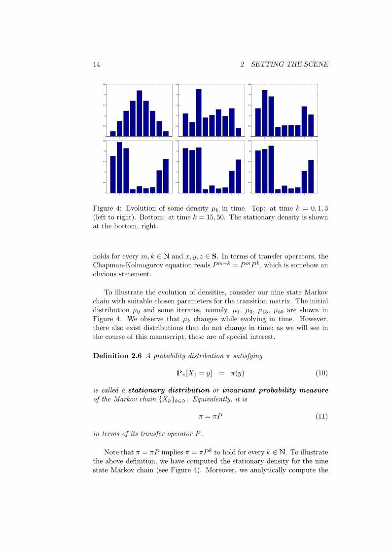
Figure 4: Evolution of some density µk in time. Top: at time k = 0, 1, 3(left to right). Bottom: at time k = 15, 50. The stationary density is shownat the bottom, right.
holds for every m,k ∈ N and x, y, z ∈ S. In terms of transfer operators, theChapman-Kolmogorov equation reads Pm+k = PmP k, which is somehow anobvious statement.
To illustrate the evolution of densities, consider our nine state Markovchain with suitable chosen parameters for the transition matrix. The initialdistribution µ0 and some iterates, namely, µ1, µ3, µ15, µ50 are shown inFigure 4. We observe that µk changes while evolving in time. However,there also exist distributions that do not change in time; as we will see inthe course of this manuscript, these are of special interest.
Definition 2.6 A probability distribution π satisfyingPπ[X1 = y] = π(y) (10)
is called a stationary distribution or invariant probability measure
of the Markov chain Xkk∈N. Equivalently, it is
π = πP (11)
in terms of its transfer operator P .
Note that π = πP implies π = πP k to hold for every k ∈ N. To illustratethe above definition, we have computed the stationary density for the ninestate Markov chain (see Figure 4). Moreover, we analytically compute the

2.4 The evolution of distributions under the Markov chain 15
stationary distribution of the two state Markov chain. Here, π = (π(1), π(2))has to satisfy
π = π
(
1− a ab 1− b
)
resulting in the two equations
π(1) = π(1)(1 − a) + π(2)b
π(2) = π(1)a + π(2)(1 − b).
This is a dependent system reducing to the single equation π(1)a = π(2)b,to which the additional constraint π(1) + π(2) = 1 must be added (why?).We obtain
π =
(
b
a + b,
a
a + b
)
.
Stationary distributions need neither to exist (as we will see below) northey need to be unique! As an example for the latter statement, consider aMarkov chain with the identity matrix as transition function. Then, everyprobability distribution is stationary.
When calculating stationary distributions, two strategies can be quiteuseful. The first one is based on the interpretation of eq. (10) as an eigen-value problem, the second one is based on the notion of the probability flux.While we postpone the eigenvalue interpretation, we will now exploit theprobability flux idea in order to calculate the stationary distribution of therandom walk on N.
Assume that the Markov chain exhibits a stationary distribution π andlet A,B ⊂ S denote two subsets of the state space. Then, the probabilityflux from A to B is defined by
fluxπ(A,B) = Pπ[X1 ∈ B,X0 ∈ A] (12)
=∑
x∈A
π(x)P (x,B) =∑
x∈A
∑
y∈B
π(x)P (x, y).
For a Markov chain possessing a stationary distribution, the flux from somesubset A to its complement Ac is somehow balanced:
Theorem 2.7 ([3]) Let Xkk∈N denote a Markov chain with stationarydistribution π and A ⊂ S an arbitrary subset of the state space. Then
fluxπ(A,Ac) = fluxπ(Ac, A),
hence the probability flux from A to its complement Ac is equal to the reverseflux from Ac to A.

16 2 SETTING THE SCENE
Proof: The proof is left as an exercise.
Now, we want to exploit the above theorem to calculate the stationarydistribution of the random walk on N. For sake of illustration, we takeak = p ∈ (0, 1) for k ∈ N. Hence, with probability p the Markov chainmoves to the right, while with probability 1 − p it moves to the left (withexception of the origin). Then, the equation of stationarity (10) reads
π(0) = π(0)(1 − p) + π(1)(1 − p) and
π(k) = π(k − 1)p + π(k + 1)(1 − p)
for k > 0. The first equation can be rewritten as π(1) = π(0)p/(1 − p).Instead of exploiting the second equation (try it), we use Theorem 2.7 toproceed. For some k ∈ N consider A = 0, . . . , k implying Ac = k +1, k +2, . . .; then
fluxπ(A,Ac) =∑
x∈A
π(x)P (x,Ac) = π(k)p
fluxπ(Ac, A) =∑
x∈Ac
π(x)P (x,A) = π(k + 1)(1 − p)
It follows from Theorem 2.7, that
π(k)p = π(k + 1)(1 − p)
and therefore
π(k + 1) = π(k)
(
p
1− p
)
= . . . = π(0)
(
p
1− p
)k+1
.
The value of π(0) is determined by demanding that π is a probability dis-tribution:
1 =∞∑
k=0
π(k) = π(0)∞∑
k=0
(
p
1− p
)k
.
Depending on the parameter p, we have
∞∑
k=0
(
p
1− p
)k
=
∞; if p ≥ 1/2
(1− p)/(1− 2p); if p < 1/2.(13)
Thus, we obtain for the random walk on N the following dependence onthe parameter p:
• for p < 1/2, the stationary distribution is given by
π(0) =1− 2p
1− pand π(k) = π(0)
(
p
1− p
)k

2.5 Some key questions concerning Markov chains 17
• for p ≥ 1/2 there does not exist a stationary distribution π, since thenormalisation in eq. (13) fails.
A density or measure π satisfying π = πP , without the requirement∑
π(x) = 1, is called invariant. Trivially, every stationary distribution isinvariant, but the reverse statement is not true. Hence, for p ≥ 1/2, thefamily of mesures π with π(0) ∈ R+ and π(k) = π(0)p/(1− p) are invariantmeasures of the random walk on N (with parameter p) .
2.5 Some key questions concerning Markov chains
1. Existence of unique invariant measure and corresponding convergencerates
µn −→ π or Pn = 1πt +O(nm2 |λ2|n).
1 2 3 4 5 6 7 8 90
0.05
0.1
0.15
0.2
0.25
1 2 3 4 5 6 7 8 90
0.05
0.1
0.15
0.2
0.25
1 2 3 4 5 6 7 8 90
0.05
0.1
0.15
0.2
0.25
1 2 3 4 5 6 7 8 90
0.05
0.1
0.15
0.2
0.25
1 2 3 4 5 6 7 8 90
0.05
0.1
0.15
0.2
0.25
2. Evaluation of expectation values and corresponding convergence rates,including sampling of the stationary distribution
1
n
n∑
k=1
f(Xk) −→∑
x∈S
f(x)π(x)
3. Identification of macroscopic properties like, e.g., cyclic or metastablebehaviour, coarse graining of the state space.

18 2 SETTING THE SCENE
4. Calculation of return and stopping times, exit probabilities and prob-abilities of absorption.
σD(x) = inft > 0 : Xt /∈ D,X0 = x
0 20 40 60 80 1000
0.2
0.4
0.6
0.8
1limit decay rate = 0.0649
time
exit tim
e d
istr
ibution

19
3 Communication and recurrence
3.1 Irreducibility and (A)periodicity
This section is about the topology of Markov chains. We start with some
Definition 3.1 Let Xkk∈N denote a Markov chain with transition func-tion P , and let x, y ∈ S denote some arbitrary pair of states.
1. The state x has access to the state y, written x→ y, ifP[Xm = y|X0 = x] > 0
for some m ∈ N that possibly depends on x and y. In other words, itis possible to move (in m steps) from x to y with positive probability.
2. The states x and y communicate, if x has access to y and y accessto x, denoted by x↔ y.
3. The Markov chain (equivalently its transition function) is said to beirreducible, if all pairs of states communicate.
The communication relation ↔ can be exploited to analyze the Markovchain in more detail. It is easy to prove that communication relation is aso–called equivalence relation, hence it is
1. reflexive: x↔ x
2. symmetric: x↔ y implies y ↔ x,
3. transitive: x↔ y and y ↔ z imply x↔ z.
Recall that every equivalence relation induces a partition S = C0∪· · ·∪Cr−1
of the state space S into so–called equivalence classes defined as
Ck = [xk] := y ∈ S : y ↔ xk
for k = 0, . . . , r − 1 and suitable states x0, . . . , xr−1 ∈ S. In the theory ofMarkov chains, the elements C0, . . . , Cr−1 of the induced partition are calledcommunication classes.
Why are we interested in communication classes? The partition intocommunication classes allows to break down the Markov chain into easierto handle and separately analyzable subunits. This might be interpretedas finding some normal form for the Markov chain. If there is only onecommunication class, hence all states communicate, then nothing can befurther partitioned, and the Markov chain is already in its normal form.There are some additional properties of communication classes:
20 3 COMMUNICATION AND RECURRENCE
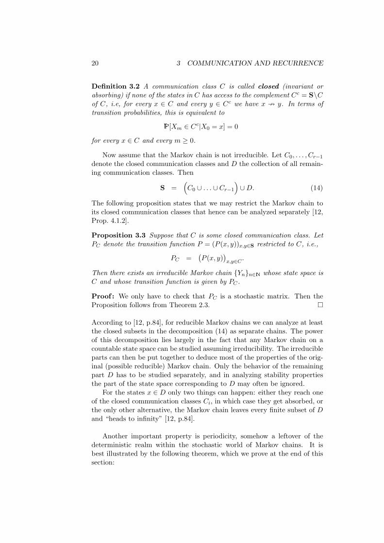
Definition 3.2 A communication class C is called closed (invariant orabsorbing) if none of the states in C has access to the complement Cc = S\Cof C, i.e, for every x ∈ C and every y ∈ Cc we have x 9 y. In terms oftransition probabilities, this is equivalent toP[Xm ∈ Cc|X0 = x] = 0
for every x ∈ C and every m ≥ 0.
Now assume that the Markov chain is not irreducible. Let C0, . . . , Cr−1
denote the closed communication classes and D the collection of all remain-ing communication classes. Then
S =(
C0 ∪ . . . ∪ Cr−1
)
∪D. (14)
The following proposition states that we may restrict the Markov chain toits closed communication classes that hence can be analyzed separately [12,Prop. 4.1.2].
Proposition 3.3 Suppose that C is some closed communication class. LetPC denote the transition function P = (P (x, y))x,y∈S restricted to C, i.e.,
PC =(
P (x, y))
x,y∈C.
Then there exists an irreducible Markov chain Ynn∈N whose state space isC and whose transition function is given by PC .
Proof : We only have to check that PC is a stochastic matrix. Then theProposition follows from Theorem 2.3.
According to [12, p.84], for reducible Markov chains we can analyze at leastthe closed subsets in the decomposition (14) as separate chains. The powerof this decomposition lies largely in the fact that any Markov chain on acountable state space can be studied assuming irreducibility. The irreducibleparts can then be put together to deduce most of the properties of the orig-inal (possible reducible) Markov chain. Only the behavior of the remainingpart D has to be studied separately, and in analyzing stability propertiesthe part of the state space corresponding to D may often be ignored.
For the states x ∈ D only two things can happen: either they reach oneof the closed communication classes Ci, in which case they get absorbed, orthe only other alternative, the Markov chain leaves every finite subset of Dand “heads to infinity” [12, p.84].
Another important property is periodicity, somehow a leftover of thedeterministic realm within the stochastic world of Markov chains. It isbest illustrated by the following theorem, which we prove at the end of thissection:

3.1 Irreducibility and (A)periodicity 21
D
C2
C1
C0
P =
Figure 5: Normal form of the transition function for r = 3.
Theorem 3.4 (cyclic structure [2]) For any irreducible Markov chainXkk∈N, there exists a unique partition of the state space S into d so–calledcyclic classes E0, . . . , Ed−1 such thatP[X1 ∈ Ek+1|X0 = x] = 1
for every x ∈ Ek and k = 0, . . . , d − 1 (by convention Ed = E0). Moreover,d is maximal in the sense that there exists no partition into more than dclasses with the same property.
Hence the Markov chain moves cyclically in each time step from oneclass to the next. The number d in Theorem 3.4 is called the period ofthe Markov chain (respectively the transition function). If d = 1, then theMarkov chain is called aperiodic. Later on, we will see, how to identify(a)periodic behavior and, for d > 1 the cyclic classes.
The transition matrix of a periodic irreducible Markov chain has a specialstructure. After renumbering of the states of S (if necessary), the transitionfunction has a block structure as illustrated in Fig. 6. There is a morearithmetic but much less intuitive definition of the period that in additiondoes not rely on irreducibility of the Markov chain.
Definition 3.5 ([2]) The period d(x) of some state x ∈ S is defined as
d(x) = gcdk ≥ 1 : P[Xk = x|X0 = x] > 0,
with the convention d(x) = ∞, if P[Xk = x|X0 = x] = 0 for all k ≥ 1. Ifd(x) = 1, then the state x is called aperiodic.
Hence, different states may have different periods. As the followingtheorem states, this is only possible for reducible Markov chains [2].

22 3 COMMUNICATION AND RECURRENCE
P = E1
E2
E0
Figure 6: Block structure of a periodic, irreducible Markov chain with periodd = 3.
Theorem 3.6 The period is a class property, i.e., all states of a communi-cation class have the same period.
Proof: Let C be a communication class and x, y ∈ C. As a consequence,there exist k,m ∈ N with P k(x, y) > 0 and Pm(y, x) > 0. Moreover,d(x) <∞ and d(y) <∞. From the Chapman-Kolmogorov Equation (9) weget
P k+j+m(x, x) ≥ P k(x, y)P j(y, y)Pm(y, x)
for all j ∈ N. Now, for j = 0 we infer that d(x) divides k + m, in shortd(x)|(k + m), since P k(x, y)Pm(y, x) > 0. Whereas choosing j such thatP j(y, y) > 0 yields d(x)|(k+ j +m). Therefore we have d(x)|j, which meansthat d(x)|d(y). By symmetry of the argument, we obtain d(y)|d(x), whichimplies d(x) = d(y).
In particular, if the Markov chain is irreducible, all states have the sameperiod d, and we may call d the period of the Markov chain (cf. Theorem 3.4).Combining Definition 3.5 with Theorem 3.6, we get the following usefulcriterion for aperiodicity:
Corollary 3.7 An irreducible Markov chain Xkk∈N is aperiodic, if thereexists some state x ∈ S such that P[X1 = x|X0 = x] > 0.
Remark. In our introductory example (random surfer on the WWW),we can easily check that the matrix P = (pw,w′)w,w′=1,...,N with
pw,w′ = P[wj+1 = w′|wj = w]
according to (1) is a stochastic matrix in which all entries are positive. Thus,the associated chain is irreducible and aperiodic.

3.1 Irreducibility and (A)periodicity 23
3.1.1 Additional Material: Proof of Theorem 3.4
We now start to prove Theorem 3.4. The proof will be a simple consequenceof the following three propositions.
Proposition 3.8 Let Xkk∈N be an irreducible Markov chain with tran-sition function P and period d. Then, for any states x, y ∈ S, there is ank0 ∈ N and m ∈ 0, . . . , d− 1, possibly depending on x and y, such that
P kd+m(x, y) > 0
for every k ≥ k0.
Proof: For now asumme that x = y, then, by the Chapman-Kolmogorovequation (9), the set Gx = k ∈ N : P k(x, x) > 0 is closed under addition,since k, k′ ∈ Gx implies
P k+k′
(x, x) ≥ P k(x, x)P k′
(x, x) > 0,
and therefore k + k′ is an element of Gx. This enables us to use a numbertheoretic result [15, Appendix A]: A subset of the natural numbers whichis closed under addition, contains all, except a finite number, multiples ofits greatest common divisor. By definition, the gcd of Gx is the period d,so there is a k0 ∈ N with P kd(x, x) > 0 for k ≥ k0. Now, if x 6= y thenirreducibility of the Markov chain ensures that there is an m ∈ N withPm(x, y) > 0 and therefore
P kd+m(x, y) ≥ P kd(x, x)Pm(x, y) > 0
for k ≥ k0. Of course k0 can be chosen in such a way that m < d.
Proposition 3.8 can be used to define an equivalence relation on S, whichgives rise to the cyclic classes in Theorem 3.4: Fix an arbitrary state z ∈ Sand define x and y to be equivalent, denoted by x ↔z y, if there is anm ∈ 0, . . . , d− 1 and an k0 ∈ N such that
P kd+m(z, x) > 0 and P kd+m(z, y) > 0
for every k ≥ k0. The relation x↔z y is indeed an equivalent relation (theproof is left as an exercise) and therefore defines a disjoint partition of thestate space S = E0 ∪ E1 ∪ E2 ∪ . . . Ed−1 with
Em = x ∈ S : P kd+m(z, x) > 0 for k ≥ k0
for m = 0, . . . , d−1. The next proposition confirms that these are the cyclicclasses used in Theorem 3.4.

24 3 COMMUNICATION AND RECURRENCE
Proposition 3.9 Let P denote the transition function of an irreducibleMarkov chain with period d and define E0, . . . , Ed−1 as above.
If P r(x, y) > 0 for some r > 0 and x ∈ Em then y ∈ Em+r, where theindices are taken modulo d. In particular, if P (x, y) > 0 and x ∈ Em theny ∈ Em+1 with the convention Ed = E0.
Proof : Let P r(x, y) > 0 and x ∈ Em, then there is a k0, such thatP kd+m(z, x) > 0 for all k ≥ k0, and hence
P kd+m+r(z, y) ≥ P kd+m(z, x)P r(x, y) > 0,
for every k > k0, therefore y ∈ Em+r.
There is one thing left to do: We have to prove that the partition of Sinto cyclic classes is unique, i.e., it does not depend on the z ∈ S chosen todefine ↔z.
Proposition 3.10 For two given states z, z′ ∈ S, the partitions of the statespace induced by ↔z and ↔z′ are equal.
Proof: Let Em and E′m′ denote two arbitrary subsets from the partitions
induced by ↔z and ↔z′ , respectively. We prove that the two subsets areeither equal or disjoint. Assume that Em and E′
m′ are not disjoint andconsider some x ∈ Em ∩ E′
m′ . Consider some y ∈ Em. Then, due toProps. 3.8 there exist k0 ∈ N and s < d such that P kd+s(x, y) > 0 fork ≥ k0. Due to 3.9, we infer y ∈ E(kd+s)+m, hence s is a multiple of d.
Consequently, P kd(x, y) > 0 for k ≥ k′′0 . By definition of E′
m′ , there is ank′0 ∈ N, such that P kd+m′
(z′, x) > 0 for k ≥ k′0, and therefore
P (k+k′′
0 )d+m′
(z′, y) ≥ P kd+m′
(z′, x)P k′′
0 d(x, y) > 0
for k ≥ k′0. Equivalently, P k′d+m′
(z′, y) > 0 for k′ ≥ k′0+k′′
0 , so that y ∈ E′m′ .
3.2 Recurrence and the existence of stationary distributions
In Section 3.1 we have investigated the topology of a Markov chain. Re-currence and transience is somehow the next detailed level of investigation.It is in particular suitable to answer the question, whether a Markov chainadmits a unique stationary distribution.
Consider an irreducible Markov chain on the state space S = N. Bydefinition we know that each two states communicate. Hence, given x, y ∈ Sthere is always a positive probability to move from x to y and vice versa.

3.2 Recurrence and the existence of stationary distributions 25
Consequently, there is also a positive probability to start in x and returnto x via visiting y. However, there might also exist the possibility thatthe Markov chain never returns to x within finite time. This is often anundesirable feature; in a sense the Markov chain is unstable.
A better notion of stability is that of recurrence, when the Markov chainreturns to any state infinitely often. The strongest results are obtained,when in addition the average return time to any state is finite. We start byintroducing the necessary notions.
Definition 3.11 A random variable T : Ω→ N∪∞ is called a stopping
time w.r.t. the Markov chain Xkk∈N, if for every integer k ∈ N the eventT = k can be expressed in terms of X0,X1, . . . ,Xk.
We give two prominent examples.
Example 3.12 For every c ∈ N, the random variable T = c is a stoppingtime.
The so–called first return time plays a crucial role in the analysis ofrecurrence and transience.
Definition 3.13 The stopping time Tx : Ω→ N ∪ ∞ defined by
Tx = mink ≥ 1 : Xk = x,
with the convention Tx = ∞, if Xk 6= x for all k ≥ 1, is called the first
return time to state x.
Note that Tx is a random variable. Hence, for a given realization ω withX0(ω) = y for some initial state y ∈ S, the term
Tx(ω) = mink ≥ 1 : Xk(ω) = x
is an integer, or infinite. Using the first return time, we can specify howoften and how likely the Markov chain returns to some state x ∈ S. Thefollowing considerations will be of use:
• The probability of starting initially in x ∈ S and returning to x inexactly n steps: Px[Tx = n].
• The probability of starting initially in x ∈ S and returning to x in afinite number of steps: Px[Tx <∞].
• The probability of starting initially in x ∈ S and not returning to x ina finite number of steps: Px[Tx =∞].

26 3 COMMUNICATION AND RECURRENCE
Of course, the relation among the three above introduced probabilities isPx[Tx <∞] =
∞∑
n=1
Px[Tx = n] and Px[Tx <∞] +Px[Tx =∞] = 1.
We now introduce the important concept of recurrence. We begin bydefining a recurrent state, and then show that recurrence is actually a classproperty, i.e., the states of some communication class are either all recurrentor none of them is.
Definition 3.14 Some state x ∈ S is called recurrent ifPx[Tx <∞] = 1,
and transient otherwise.
The properties of recurrence and transience are intimately related to thenumber of visits to a given state. To do so, we need a generalization of theMarkov property, the so-called strong Markov property. It states thatthe Markov property, i.e. the independence of past and future given thepresent state, holds even if the present state is determined by a stoppingtime.
Theorem 3.15 (Strong Markov property) Let Xkk∈N be a homoge-nous Markov chain on a countable state space S with transition matrix P andinitial distribution µ0. Let T denote a stopping time w.r.t. the Markov chain.Then, conditional on T <∞ and XT = z ∈ S, the sequence (XT+n)n∈N is aMarkov chain with transition matrix P and initial state z that is independentof X0, . . . ,XT .
Proof: Let H ⊂ Ω denote some event determined by X0, . . . ,XT , e.g., H =X0 = y0, . . . ,XT = yT for y0, . . . , yT ∈ S. Then, the event H ∩ T = mis determined by X0, . . . ,Xm. By the Markov property at time t = m weget Pµ0 [XT = x0, . . . ,XT+n = xn,H,XT = z, T = m]
= Pµ0 [XT = x0, . . . ,XT+n = xn|H,Xm = z]Pµ0 [H,XT = z, T = m]
= Pz[X0 = x0, . . . ,Xn = xn]Pµ0 [H,XT = z, T = m].
Hence, summation over m = 0, 1, . . . yieldsPµ0 [XT = x0, . . . ,XT+n = xn,H,XT = z, T <∞]
= Pz[X0 = x0, . . . ,Xn = xn]Pµ0 [H,XT = z, T <∞],

3.2 Recurrence and the existence of stationary distributions 27
and dividing by Pµ0 [XT = z, T <∞], we finally obtainPµ0 [XT = x0, . . . ,XT+n = xn,H|XT = z, T <∞]
= Pz[X0 = x0, . . . ,Xn = xn]Pµ0 [H|XT = z, T <∞].
This is exactly the statement of the strong Markov property.
Theorem 3.15 states that if a Markov chain is stopped by any “stoppingtime rule” at, say XT = x, and the realization after T is observed, it cannot be distinguished from the Markov chain started at x (with the sametransition function, of course). Now, we are ready to state the relationbetween recurrence and the number of visits Ny : Ω → N ∪ ∞ to somestate y ∈ S defined by
Ny =
∞∑
k=1
1Xk=y.
Exploiting the strong Markov property and by induction [2, Thm. 7.2], itcan be shown thatPx[Ny = m] = Px[Ty <∞]Py[Ty <∞]m−1Py[Ty =∞] (15)
for m > 0, and Px[Ny = 0] = Px[Ty =∞].
Theorem 3.16 Consider some state x ∈ S. Then
x is recurrent⇔ Px[Nx =∞] = 1⇔ Ex[Nx] =∞,
and
x is transient⇔ Px[Nx =∞] = 0⇔ Ex[Nx] <∞.
The above equivalence in general fails to hold for the denumerable, moregeneral state space case—here, one has to introduce the notion of Harrisrecurrent [12, Chapt. 9].
Proof: Now, if x is recurrent then Px[Tx <∞] = 1. Hence, due to eq. (15)Px[Nx <∞] =
∞∑
m=0
Px[Nx = m] =
∞∑
m=0
Px[Tx <∞]mPx[Tx =∞],
vanishes, since every summand is zero. Consequently, Px[Nx = ∞] = 1.Now, if x is transient, then Px[Tx <∞] < 1 and hencePx[Nx <∞] = Px[Tx =∞]
∞∑
m=0
Px[Tx <∞]m =Px[Tx =∞]
1−Px[Tx <∞]= 1.

28 3 COMMUNICATION AND RECURRENCE
FurthermoreEx[Nx] =
∞∑
m=1
mPx[Nx = m] =
∞∑
m=1
mPx[Tx <∞]mPx[Tx =∞]
= Px[Tx <∞]Px[Tx =∞]d
dPx[Tx <∞]
∞∑
m=1
Px[Tx <∞]m
= Px[Tx <∞]Px[Tx =∞]d
dPx[Tx <∞]
1
1−Px[Tx <∞]
=Px[Tx <∞]Px[Tx =∞]
(1−Px[Tx <∞])2=
Px[Tx <∞]
1−Px[Tx <∞].
Hence, Ex[Nx] <∞ implies Px[Tx <∞] < 1, and vice versa. The remainingimplications follow by negation.
A Markov chain may possess both, recurrent and transient states as,e.g., the two state Markov chain given by
P =
(
1− a a0 1
)
.
for some a ∈ (0, 1). This example is actually a nice illustration of the nextproposition.
Proposition 3.17 Consider a Markov chain Xkk∈N on a state space S.
1. If Xkk∈N admits some stationary distribution π and y ∈ S is sometransient state then π(y) = 0.
2. If the state space S is finite, then there exists at least some recurrentstate x ∈ S.
Proof: 1. Assume we had proven that Ex[Ny] <∞ for arbitrary x ∈ S andtransient y ∈ S, which implies P k(x, y)→ 0 for k →∞. Then
π(y) =∑
x∈S
π(x)P k(x, y)
for every k ∈ N, and finally
π(y) = limk→∞
∑
x∈S
π(x)P k(x, y) =∑
x∈S
π(x) limk→∞
P k(x, y) = 0.
where exchanging summation and limit is justified by the theorem of domi-nated convergence (e.g., [2, Appendix]), which proves the statement. Hence,it remains to prove Ex[Ny] <∞.

3.2 Recurrence and the existence of stationary distributions 29
If Py[Ty < ∞] = 0, then Ex[Ny] = 0 < ∞. Now assume that Py[Ty <∞] > 0. Then, we obtainEx[Ny] =
∞∑
m=1
mPx[Ty <∞]Py[Ty <∞]m−1Py[Ty =∞]
=Px[Ty <∞]Py[Ty <∞]
Ey[Ny] <∞
where the last inequality is due to transience of y and Thm. 3.16.2. Proof left as an excercise (Hint: Use Proposition 3.17 and think on
properties of stochastic matrices).
The following theorem gives some additional insight into the relationbetween different states. It states that recurrence and transience are classproperties.
Theorem 3.18 Consider two states x, y ∈ S that communicate. Then
1. If x is recurrent then y is recurrent;
2. If x is transient then y is transient.
Proof: Since x and y communicate, there exist integers m,n ∈ N such thatPm(x, y) > 0 and Pn(y, x) > 0. Introducing q = Pm(x, y)Pn(y, x) > 0,and exploiting the Chapman-Kolmogorov equation, we get Pn+k+m(x, x) ≥Pm(x, y)P k(y, y)Pn(y, x) = qP k(y, y) and Pn+k+m(y, y) ≥ qP k(x, x), fork ∈ N. Consequently,Ey[Ny] = Ey
[
∞∑
k=1
1Xk=y
]
=
∞∑
k=1
Ey[1Xk=y] =
∞∑
k=1
Py[Xk = y]
=
∞∑
k=1
P k(y, y) ≤ 1
q
∞∑
k=m+n
P k(x, x) ≤ 1
qEx[Nx].
Analogously, we get Ex[Nx] ≤ Ey[Ny]/q. Now, the two statements directlyfollow by Thm. 3.16.
As a consequence of Theorem 3.18, all states of an irreducible Markovchain are of the same nature: We therefore call an irreducible Markov chainrecurrent or transient, if one of its states (and hence all) is recurrent, re-spectively, transient. Let us summarize the stability properties introducedso far. Combining Theorem 3.18 and Prop. 3.17 we conclude:
• Given some finite state space Markov chain
(i) that is not irreducible: there exists at least one recurrent com-munication class that moreover is closed.

30 3 COMMUNICATION AND RECURRENCE
(ii) that is irreducible: all states are recurrent, hence so is the Markovchain.
• Given some countable infinite state space Markov chain
(i) that is not irreducible: there may exist recurrent as well as tran-sient communication classes.
(ii) that is irreducible: all states are either recurrent or transient.
We now address the important question of existence and uniquenessof invariant measures and stationary distributions. The following theoremstates that for irreducible and recurrent Markov chains there always existsa unique invariant measure (up to a multiplicative factor).
Theorem 3.19 Consider an irreducible and recurrent Markov chain. Foran arbitrary state x ∈ S define µ =
(
µ(y))
y∈Swith
µ(y) = Ex
[
Tx∑
n=1
1Xn=y
]
, (16)
the expected value for the number visits in y before returning to x. Then
1. 0 < µ(y) < ∞ for all y ∈ S. Moreover, µ(x) = 1 for the state x ∈ Schosen in the eq. (16).
2. µ = µP .
3. If ν = νP for some measure ν, then ν = αµ for some α ∈ R.
The interpretation of eq. (16) is this: for some fixed x ∈ S the invariantmeasure µ(y) is proportional to the number of visits to y before returningto x. Note that the invariant measure µ defined in (16) in general dependson the state x ∈ S chosen, since µ(x) = 1 per construction. This reflects thefact that µ is only determined up to some multiplicative factor (stated in(iii)). We further remark that eq. (16) defines for every x ∈ S some invari-ant distribution, however for some arbitrarily given invariant measure µ, ingeneral there does not exist an x ∈ S such that eq. (16) holds.
Proof: 1. Note that due to recurrence of x and definition of µ we have
µ(x) = Ex
[
Tx∑
n=1
1Xn=x
]
=
∞∑
n=1
Ex[1Xn=x1n≤Tx]
=
∞∑
n=1
Px[Xn = x, n ≤ Tx] =
∞∑
n=1
Px[Tx = n] = Px[Tx <∞] = 1,

3.2 Recurrence and the existence of stationary distributions 31
which proves µ(x) = 1. We postpone the second part of the first statementand prove
2. Observe that for n ∈ N, the event Tx ≥ n depends only on therandom variables X0,X1, . . . ,Xn−1. ThusPx[Xn = z,Xn−1 = y, Tx ≥ n] = Px[Xn−1 = y, Tx ≥ n]P (y, z).
Now, we have for arbitrary z ∈ S∑
y∈S
µ(y)P (y, z) = µ(x)P (x, z) +∑
y 6=x
µ(y)P (y, z)
= P (x, z) +∑
y 6=x
∞∑
n=1
Px[Xn = y, n ≤ Tx]P (y, z)
= P (x, z) +∞∑
n=1
∑
y 6=x
Px[Xn+1 = z,Xn = y, n ≤ Tx]
= Px[X1 = z] +∞∑
n=1
Px[Xn+1 = z, n + 1 ≤ Tx]
= Px[X1 = z, 1 ≤ Tx] +
∞∑
n=2
Px[Xn = z, n ≤ Tx]
=∞∑
n=1
Px[Xn = z, n ≤ Tx] = µ(z),
where for the second equality we used µ(x) = 1 and for the fourth equalitywe used that Xn = y, n ≤ Tx and x 6= y implies n+1 ≤ Tx. Thus we provedµP = µ.
1. (continued) Since P is irreducible, there exist integers k, j ∈ N suchthat P k(x, y) > 0 and P j(y, x) > 0 for every y ∈ S. Therefore, for everyk ∈ N and exploiting statement 2.), we have
0 < µ(x)P k(x, y) ≤∑
z∈S
µ(z)P k(z, y) = µ(y).
On the other hand,
µ(y) =µ(y)P j(y, x)
P j(y, x)≤∑
z∈Sµ(z)P j(z, x)
P j(y, x)=
µ(x)
P j(y, x)<∞.
Hence, the first statement has been proven.3. The first step to prove the uniqueness of µ is to show that µ is minimal,
which means that ν ≥ µ holds for any other invariant measure ν satisfyingν(x) = µ(x) = 1. We prove by induction that
ν(z) ≥k∑
n=1
Px[Xn = z, n ≤ Tx] (17)
32 3 COMMUNICATION AND RECURRENCE
holds for every z ∈ S. Note that the right hand side of eq. (17) convergesto µ(z) as k →∞ (cmp. proof of 1.). For k = 1 it is
ν(z) =∑
y∈S
ν(y)P (y, z) ≥ P (x, z) = Px[X1 = z, 1 ≤ Tx].
Now, assume that eq. (17) holds for some k ∈ N. Then
ν(z) ≥ ν(x)P (x, z) +∑
y 6=x
ν(y)P (y, z)
≥ P (x, z) +∑
y 6=x
k∑
n=1
Px[Xn = y, n ≤ Tx]P (y, z)
= Px[X1 = z, 1 ≤ Tx] +k∑
n=1
Px[Xn+1 = z, n + 1 ≤ Tx]
=
k+1∑
n=1
Px[Xn = z, n ≤ Tx].
Therefore, eq. (17) holds for every k ∈ N, and in the limit we get ν ≥ µ.Define λ = ν − µ; since P is irreducible, for every z ∈ S there exists someinteger k ∈ N such that P k(z, x) > 0. Thus
0 = λ(x) =∑
y∈S
λ(y)P k(y, x) ≥ λ(z)P k(z, x),
implying λ(z) = 0 and finally ν = µ. Now, if we relax the condition ν(x) = 1,then statement 3. follows with c = ν(x).
We already know that the converse of Theorem 3.19 is false, since thereare transient irreducible Markov chains that possess invariant measures. Forexample, the random walk on N is transient for p > 1/2, but admits aninvariant measure. At the level of invariant measures, nothing more canbe said. However, if we require that the invariant measure is a probabilitymeasure, then it is possible to give necessary and sufficient conditions. Theseinvolve the expected return timesEx[Tx] =
∞∑
n=1
nPx[Tx = n]. (18)
Depending on the behavior of Ex[Tx], we further distinguish two types ofstates:
Definition 3.20 A recurrent state x ∈ S is called positive recurrent, ifEx[Tx] < ∞and null recurrent otherwise.

3.2 Recurrence and the existence of stationary distributions 33
In view of eq. (18) the difference between positive and null recurrence ismanifested in the decay rate of Px[Tx = n] for n → ∞. If Px[Tx = n]decays too slowly as n → ∞, then Ex[Tx] is infinite and the state is nullrecurrent. On the other hand, if Px[Tx = n] decays rapidly in the limitn→∞, then Ex[Tx] will be finite and the state is positive recurrent.
As for recurrence, positive and null recurrence are class properties [2].Hence, we call a Markov chain positive or null recurrent, if one of its states(and therefore all) is positive, respectively, null recurrent. The next theoremillustrates the usefulness of positive recurrence and gives an additional usefulinterpretation of the stationary distribution.
Theorem 3.21 Consider an irreducible Markov chain. Then the Markovchain is positive recurrent, if and only if there exists a stationary distri-bution. Under these conditions, the stationary distribution is unique andpositive everywhere, with
π(x) =1Ex[Tx]
.
Hence π(x) can be interpreted as the inverse of the expected first return timeto state x ∈ S.
Proof: Theorem 3.19 states that an irreducible and recurrent Markov chainadmits an invariant measure µ defined through (16) for an arbitrary x ∈ S.Thus
∑
y∈S
µ(y) =∑
y∈S
Ex
[
Tx∑
n=1
1Xn=y
]
= Ex
∞∑
n=1
∑
y∈S
1Xn=y1n≤Tx
= Ex
[
∞∑
n=1
1n≤Tx
]
=
∞∑
n=1
Px[Tx ≥ n]
=
∞∑
n=1
∞∑
k=n
Px[Tx = k] =
∞∑
k=1
kPx[Tx = k] = Ex[Tx],
which is by definition finite in the case of positive recurrence. Therefore thestationary distribution can be obtained by normalization of µ with Ex[Tx]yielding
π(x) =µ(x)Ex[Tx]
=1Ex[Tx]
.
Since the state x was chosen arbitrary this is true for all x ∈ S. Uniquenessand positivity of π follows from Theorem 3.19. On the other hand, if thereexists a stationary distribution the Markov process must be recurrent be-cause otherwise π(x) would be zero for all x ∈ S according to Theorem 3.17.Positive recurrence follows from the uniqueness of π and the consideration
34 3 COMMUNICATION AND RECURRENCE
above.
Our considerations in the proof of Theorem 3.21 easily leads to a criteriato distinguish positive recurrence from null recurrence.
Corollary 3.22 Consider an irreducible recurrent Markov chain Xkk∈Nwith invariant measure µ = (µ(x))x∈S. Then
1. Xkk∈N positive recurrent ⇔ ∑
x∈S
µ(x) <∞,
2. Xkk∈N null recurrent ⇔ ∑
x∈S
µ(x) =∞.
Proof: The proof is left as an exercise.
For the finite state space case, we have the following powerful statement.
Theorem 3.23 Every irreducible Markov chain on a finite state space ispositive recurrent and therefore admits a unique stationary distribution thatis positive everywhere.
Proof: The proof is left as an exercise.
For the general possibly non-irreducible case, the results of this sectionare summarized in the next
Proposition 3.24 Let C ⊂ S denote a communication class correspondingto some Markov chain Xkk∈N on the state space S.
1. If C is not closed, then all states in C are transient.
2. If C is closed and finite, then all states in C are positive recurrent.
3. If all state in C are null recurrent, then C is necessarily infinite.
Proof: The proof is left as an exercise.
Remark. In our introductory example (random surfer on the WWW)we considered the transition matrix P = (pw,w′)w,w′=1,...,N with
pw,w′ = P[wj+1 = w′|wj = w]
according to (1). The associated chain is irreducible (one closed commu-nication class), aperiodic and positive recurrent. Its stationary distribu-tion π thus is unique, positive everywhere and given by either πP = π orπ(w) = 1/Ew[Tw]. The value π(w) is a good candidate for the probabilitypw of a visit of the average surfer on webpage w ∈ 1, . . . , N. That this isin fact true will be shown in the next chapter.

3.2 Recurrence and the existence of stationary distributions 35
Figure 7: Different recurrent behavior of irreducible, aperiodic Markovchains.

36 4 ASYMPTOTIC BEHAVIOR
4 Asymptotic behavior
The asymptotic behavior of distributions and transfer operators is closelyrelated to so-called ergodic properties of the Markov chain. The term er-godicity is not consistently used in literature. In ergodic theory, it roughlyrefers to the fact that space and time averages coincide (as, e.g., stated inthe strong law of large numbers by Thm. 5.1). In the theory of Markovchain, however, the meaning is slightly different. Here, ergodicity is relatedto the convergence of probability distributions ν0 in time, i.e., νk → π ask →∞, and assumes aperiodicity as a necessary condition.
4.1 k-step transition probabilities and distributions
We prove statements for the convergence of k-step probabilities involvingtransient, null recurrent and finally positive recurrent states.
Proposition 4.1 Let y ∈ S denote a transient state of some Markov chainwith transition function P . Then, for any initial state x ∈ S
P k(x, y)→ 0
as k →∞. Hence, the y-th column of P k tends to zero as k →∞.
Proof: This has already been proved in the proof of Prop. 3.17
The situation is similar for an irreducible Markov chain that is null re-current (and thus defined on a infinite countable state space due to Theo-rem 3.23):
Theorem 4.2 (Orey’s Theorem) Let Xkk∈N be an irreducible null re-current Markov chain on S. Then, for all pairs of states x, y ∈ S
P k(x, y)→ 0
as k →∞.
Proof: See, e.g., [2], p.131.
In order to derive a result for the evolution of k-step transition proba-bilities for positive recurrent Markov chains, we will exploit a powerful toolfrom probability theory, the coupling method (see, e.g., [9, 14]).
Definition 4.3 A coupling of two random variables X,Y : Ω → S is arandom variable Z : Ω→ S× S such that
∑
y∈S
P[Z = (x, y)] = P[X = x], and∑
x∈S
P[Z = (x, y)] = P[Y = y]

4.1 k-step transition probabilities and distributions 37
for every x ∈ S, and for every y ∈ S, respectively. Hence, the coupling Zhas X and Y as its marginals.
Note that, except for artificial cases, there exists infinitely many cou-plings of two random variables. The coupling method exploits the fact thatthe total variation distance between the two distributions P[X ∈ A] andP[Y ∈ A] can be bounded in terms of the coupling Z.
Proposition 4.4 (Basic coupling inequality) Consider two independentrandom variables X,Y : Ω→ S with distributions ν and π, respectively, de-fined via ν(x) = P[X = x] and π(y) = P[Y = y] for x, y ∈ S. Then
‖ν − π‖TV ≤ 2P[X 6= Y ],
with [X 6= Y ] = ω ∈ Ω : X(ω) 6= Y (ω).
Proof: We have for some subset A ⊂ S
|ν(A)− π(A)| = |P[X ∈ A]−P[Y ∈ A]|= |P[X ∈ A,X = Y ] +P[X ∈ A,X 6= Y ]
−P[Y ∈ A,X = Y ]−P[Y ∈ A,X 6= Y ]|= |P[X ∈ A,X 6= Y ]−P[Y ∈ A,X 6= Y ]|≤ P[X 6= Y ].
Since‖ν − π‖TV = 2 sup
A⊂S
|ν(A)− π(A)|
the statement directly follows.
Note that the term P[X 6= Y ] in the basic coupling inequality can bestated in terms of the coupling Z:P[X 6= Y ] =
∑
x,y∈S,x 6=y
P[Z = (x, y)] = 1−∑
x∈S
P[Z = (x, x)].
Since there are many couplings the aim is two construct a coupling Z suchthat
∑
x 6=yP[Z = (x, y)] is as small, or∑
xP[Z = (x, x)] is as large aspossible. To prove convergence results for the evolution of the distributionof some Markov chain, we exploit a specific (and impressive) example of thecoupling method.
Consider an irreducible, aperiodic, positive recurrent Markov chain X =Xkk∈N with stationary distribution π and some initial distribution ν0.Moreover, define another independent Markov chain Y = Ykk∈N thathas the same transition function as X, but the stationary distribution π as

38 4 ASYMPTOTIC BEHAVIOR
initial distribution. Observe that Y is a stationary process, i.e., the induceddistribution of Yk equals π for all k ∈ N. Then, we can make use of thecoupling method by interpreting the Markov chains as random variablesX,Y : Ω → SN and consider some coupling Z : Ω → SN × SN. Define thecoupling time Tc : Ω→ N by
Tc = mink ≥ 1 : Xk = Yk;
Tc is the first time at which the Markov chains X and Y met; moreover, itis stopping time for Z. The next proposition bounds the distance betweenthe distributions νk and π at time k in terms of the coupling time Tc.
Proposition 4.5 Consider some irreducible, aperiodic, positive recurrentMarkov chain with initial distribution ν0 and stationary distribution π. Then,the distribution νk at time k satisfies
‖νk − π‖TV ≤ 2P[k < Tc]
for every k ∈ N, where Tc denote the coupling time defined above.
T k−>
S
Xk
Yk
X’
k
Figure 8: The construction of the coupled process X ′ as needed in the proofof Prop. 4.5. Here, T denotes the value of the coupling time Tc for thisrealization.
Proof: We start by defining a new stochastic process X ′ = X ′kk∈N with
X ′k : Ω→ S (see Fig. 8) according to
X ′k =
Xk; if k < Tc,
Yk; if k ≥ Tc.
Due to the strong Markov property 3.15 (applied to the coupled Markovchain (Xk, Yk)k∈N), X ′ is a Markov chain with the same transition prob-abilities as X and Y . As a consequence of the definition of X ′ we have
4.1 k-step transition probabilities and distributions 39Pν0[Xk ∈ A] = Pν0 [X′k ∈ A] for k ∈ N and every A ⊂ S, hence the distribu-
tions of Xk and X ′k are the same. Hence, from the basic coupling inequality,
we get
|νk(A) − π(A)| = |P[X ′k ∈ A]−P[Yk ∈ A]| ≤ 2P[X ′
k 6= Yk].
Since X ′k 6= Yk ⊂ k < Tc, we finally obtainP[X ′
k 6= Yk] ≤ P[k < Tc],
which implies the statement.
Proposition 4.5 enables us to prove the convergence of νk to π by provingthat P[k < Tc] converges to zero.
Theorem 4.6 Consider some irreducible, aperiodic, positive recurrent Markovchain with stationary distribution π. Then, for any initial probability distri-bution ν0, the distribution of the Markov chain at time k satisfies
‖νk − π‖TV → 0
as k → ∞. In particular, choosing the initial distribution to be a deltadistribution at x ∈ S, we obtain
‖P k(x, ·) − π‖TV → 0
as k →∞.
Proof: It suffices to prove P[Tc <∞] = 1. Moreover, if we fixe some statex∗ ∈ S and consider the stopping time
T ∗c = infk ≥ 1;Xk = x∗ = Yk,
then P[Tc < ∞] = 1 follows from P[T ∗c < ∞] = 1. To prove the latter
statement, consider the coupling Z = (Zk)k∈N with Zk = (Xk, Yk) ∈ S× Swith X = Xkk∈N and Y = Ykk∈N defined as above. Because X and Yare independent, the transition matrix PZ of Z is given by
PZ
(
(v,w), (x, y))
= P (v,w)P (x, y)
for all v,w, x, y ∈ S. Obviously, Z has a stationary distribution given by
πZ(x, y) = π(x)π(y).
Furthermore the coupled Markov chain is irreducible: consider (v,w), (x, y) ∈S×S arbitrary. Since X and Y are irreducible and aperiodic we can choose

40 4 ASYMPTOTIC BEHAVIOR
Irreducible and aperiodic
Recurrent MC
Positive recurrent Null recurrent
Markov chain
Transient MC
, x ∈ SPx[Tx <∞] < 1 Px[Tx <∞] = 1
Ex[Tx] <∞Ex[Tx] =∞P k(x, y)→ 0 ∀y ∈ S
P k(x, y)→ π(y) = 1Ey [Ty] P k(x, y)→ 0 ∀y ∈ S
1
Figure 9: Long run behaviour of an irreducible aperiodic Markov chain.
an integer k∗ > 0 such that P k∗
(v,w) > 0 and P k∗
(x, y) > 0 holds, seeProp. 3.8. Therefore
P k∗
Z
(
(v,w), (x, y))
= P k∗
(v,w)P k∗
(x, y) > 0.
Hence Z is irreducible. Finally observe that T ∗c is the first return time of the
coupled Markov chain to the state (x∗, x∗). Since Z is irreducible and has astationary distribution, it is positive recurrent according to Thm. 3.21. ByThm. 3.18, this implies P[T ∗
c < ∞] = 1, which completes the proof of thestatement.
Fig. 9 summarizes the long run behavior of irreducible and aperiodicMarkov chains.
4.2 Time reversal and reversibility
The notions of time reversal and time reversibility are very productive, inparticular w.r.t. the spectral theory, the central limit theory and theory ofMonte Carlo methods, as we will see.
Chang [3] has a nice motivation of time reversibility: Let X0,X1, . . . de-note a Markov chain with transition function P . Imagine that I recordeda movie of the sequence of states (X0, . . . ,Xn), and I am showing you themovie on my fancy machine that can play the tape forward or backwardequally well. Can you tell by watching the sequence of transitions on themovie whether I am showing it forward or backward?
To answer this question, we determine the transition probabilities of theMarkov chain Ykk∈N obtained by reversing time for the original Markov

4.2 Time reversal and reversibility 41
chain Xkk∈N. Given some probability distribution π > 0, we require thatPπ[Y0 = xm, . . . , Ym = x0] = Pπ[X0 = x0, . . . ,Xm = xm]
holds for every m ∈ N and every x0, . . . , xm ∈ S in the case of reversibility.For the special case m = 1 we havePπ[Y0 = y, Y1 = x] = Pπ[X0 = x,X1 = y] (19)
for x, y ∈ S. Denote by Q and P the transition functions of the Markovchains Yk and Xk, respectively. Then, by equation (19) we obtain
π(y)Q(y, x) = π(x)P (x, y). (20)
Note that the diagonals of P and Q are always equal, hence Q(x, x) =P (x, x) for every x ∈ S. Moreover, from eq. (20) we deduce by summingover all x ∈ S that π is some stationary distribution of the Markov chain.
Definition 4.7 Consider some Markov chain X = Xkk∈N with transitionfunction P and stationary distribution π > 0. Then, the Markov chainYkk∈N with transition function Q defined by
Q(y, x) =π(x)P (x, y)
π(y)(21)
is called the time-reversed Markov chain (assoziated with X).
Example 4.8 Consider the two state Markov chain given by
P =
(
1− a ab 1− b
)
.
for a, b ∈ [0, 1]. The two state Markov chain is an exceptionally simpleexample, since we know on the one hand that the diagonal entries of Qand P are identical, and on the other hand that Q is a stochastic matrix.Consequently Q = P .
Example 4.9 Consider a Markov chain on the state space S = 1, 2, 3given by
P =
1− a a 00 1− b bc 0 1− c
.
for a, b, c ∈ [0, 1]. Denote by π the stationary distribution (which exists dueto Theorem 3.23). Then, π = πP is equivalent to aπ(1) = bπ(2) = cπ(3). Ashort calculation reveals
π =1
ab + ac + bc
(
bc, ac, ab)
.

42 4 ASYMPTOTIC BEHAVIOR
Once again, we have only to compute the off–diagonal entries of Q. We get
Q =
1− a 0 ab 1− b 00 c 1− c
.
For illustration, consider the case a = b = c = 1. Then P is periodicwith period d = 3; it moves deterministically: 1 → 2 → 3 → 1 . . .. Byconstruction, the matrix Q corresponds to the time reversed Markov chainthat moves like: 3→ 2→ 1→ 3 . . ., but this is exactly the dynamics definedby Q.
Definition 4.10 Consider some Markov chain X = Xkk∈N with transi-tion function P and stationary distribution π > 0, and its associated time-reversed Markov chain with transition function Q. Then X is called re-
versible w.r.t. π, ifP (x, y) = Q(x, y)
for all x, y ∈ S.
The above definition can be reformulated: a Markov chain is reversiblew.r.t. π, if and only if the detailed balance condition
π(x)P (x, y) = π(y)P (y, x) (22)
is satisfied for every x, y ∈ S. Eq. (22) has a nice interpretation in termsof the probability flux defined in (12). Recall that the flux from x to y isdefined by fluxπ(x, y) = π(x)P (x, y). Thus, eq. (22) states that the flux fromx to y is the same as the flux from y to x—it is locally balanced between eachpair of states: fluxπ(x, y) = fluxπ(y, x) for x, y ∈ S. This is a much strongercondition than the global balance condition that characterizes stationarity.The global balance condition that can be rewritten as
∑
x π(y)P (y, x) =π(y) =
∑
x π(x)P (x, y) states that the total flux leaving state x is the sameas the total flux into state x: fluxπ(x,S \ x) = fluxπ(S \ x, x).
Corollary 4.11 Given some Markov chain with transition function P andstationary distribution π. If there exist a pair of states x, y ∈ S with π(x) > 0such that
P (x, y) > 0, while P (y, x) = 0
then the detailed balance condition cannot hold for P , hence the Markovchain is not reversible. This is in particular the case, if the Markov chainis periodic with period d > 2.
Application of Corollary 4.11 yields that the three state Markov chaindefined in Example 4.9 cannot be reversible.

4.3 Some spectral theory 43
Example 4.12 Consider the random walk on N with fixed parameter p ∈(0, 1
2). The Markov chain is given by
P (x, x + 1) = p and P (x + 1, x) = 1− p
for x ∈ S and P (0, 0) = 1 − p, while all other transition probabilities arezero. It is irreducible and admits a unique stationary distribution given by
π(0) =1− 2p
1− pand π(k) = π(0)
(
p
1− p
)k
for k > 0. Obviously, we expect no trouble due to Corollary 4.11. Moreover,we have
π(x)P (x, x + 1) = π(x + 1)P (x + 1, x)
for arbitrary x ∈ S; hence, the detailed balance condition holds for P andthe random walk on N is reversible.
Last but not least let us observe that the detailed balance condition canalso be used without assuming π to be a stationary distribution:
Theorem 4.13 Consider some Markov chain X = Xkk∈N with transitionfunction P and a probability distribution π > 0. Let the detailed balancecondition be formally satisfied:
π(x)P (x, y) = π(y)P (y, x).
Then, π is a stationary distribution of X, i.e., πP = π.
Proof: The statement is an easy consequence of the detailed balance con-dition and
∑
y P (x, y) = 1 for all y ∈ S:
πP (y) =∑
x∈S
π(x)P (x, y) = π(y)∑
x∈S
P (y, x) = π(y).
4.3 Some spectral theory
We now introduce the necessary notions from spectral theory in order toanalyze the asymptotic behavior of transfer operators. Throughout this sec-tion, we assume that π is some stationary distribution of a Markov chainwith transition function P . Note that π is neither assumed to be unique norpositive everywhere.

44 4 ASYMPTOTIC BEHAVIOR
We start by introducing the Banach spaces (of equivalence classes)
lr(π) = v : S→ C :∑
x∈S
|v(x)|rπ(x) <∞,
for 1 ≤ r <∞ with corresponding norms
‖v‖r =
(
∑
x∈S
|v(x)|rπ(x)
)1/r
andl∞(π) = v : S→ C : π- sup
x∈S
|v(x)| <∞,
with supremums norm defined by
‖v‖∞ = π- supx∈S
|v(x)| = supx∈S,π(x)>0
|v(x)|.
Given two functions u, v ∈ l2(π), the π–weighted scalar product 〈·, ·〉π :S× S→ C is defined by
〈u, v〉π =∑
x∈S
u(x)v(x)π(x),
where v denotes the conjugate complex of v. Note that l2(π), equipped withthe scalar product 〈·, ·〉π , is a Hilbert space.
Remark. In general, the elements of the above introduced functionspaces are equivalence classes of functions [f ] = g : S → C : g(x) =f(x), if π(x) > 0 rather than single functions f : S→ C (this is equivalentto the approach of introducing equivalence classes of Lebesgue-integrablefunctions (see, e.g., [20])). Hence, functions that differ on a set of pointswith π-measure zero are considered to be equivalent. However, if the prob-ability distribution π is positive everywhere, we regain the interpretation offunctions as elements.
Before proceeding, we need the following two definitions.
Definition 4.14 Given some Markov chain with stationary distribution π.
1. Some measuere ν ∈M is said to be absolutely continuous w.r.t. π,in short ν ≪ π, if
π(x) = 0 ⇒ ν(x) = 0
for every x ∈ S. In this case, there exists some function f : S → Csuch that ν = fπ. The function f is called the Radon-Nikodym
derivative of ν w.r.t. π and sometimes denoted by dν/dπ.

4.3 Some spectral theory 45
2. The stationary distribution π is called maximal, if every other sta-tionary distribution ν is absolutely continuous w.r.t. π.
In broad terms, a stationary distribution is maximal, if it possesses asmany non–zero elements as possible. Note that a maximal stationary dis-tribution need not be unique.
Example 4.15 Consider the state space S = 1, 2, 3, 4 and a Markov chainwith transition function
P =
1 0 0 00 1 0 00 0 1 01 0 0 0
.
Then ν1 = (1, 0, 0, 0), ν2 = (0, 1, 0, 0), ν3 = (0, 0, 1, 0) are stationary distri-butions of P , but none of them is obviously maximal. In contrast to that,both π = (1
3 , 13 , 1
3 , 0) and σ = (12 , 1
4 , 14 , 0) are maximal stationary distribu-
tions. Note that since state x = 4 is transient, every stationary distributionν satisfies ν(4) = 0 due to Proposition 3.17.
To this end, we consider some Markov chain with maximal stationarydistribution π. We now restrict the transfer operator P from the space ofcomplex finite measuresM to the space of complex finite measures that areabsolutely continuous w.r.t. π. We define for 1 ≤ r ≤ ∞
Mr(π) = ν ∈M : ν ≪ π and dν/dπ ∈ lr(π)
with corresponding norm ‖ν‖Mr(π) = ‖dν/dπ‖r. Note that ‖ν‖M1(π) =‖ν‖TV and M1(π) ⊇ M2(π) ⊇ . . .. We now define the transfer operatorP :M1(π)→M1(π) by
νP (y) =∑
x∈S
ν(x)P (x, y).
It can be shown by exploiting Holders inequality that P is well-defined onanyMr(π) for 1 ≤ r ≤ ∞.
It is interesting to note that the transfer operator P on M1(π) inducessome transfer operator P on l1(π): Given some ν ∈ M1(π) with derivativev = dν/dπ, it follows that νP ≪ π (if π is some stationary measure withπP = π then π(y) implies p(x, y) for every x ∈ S with π(x) > 0. Now, thestatement directly follows). Hence, we define P by (vπ)P = (vP)π. Moreprecisely, it is P : l1(π)→ l1(π) given by
vP(y) =∑
x∈S
Q(y, x)v(x)

46 4 ASYMPTOTIC BEHAVIOR
for v ∈ l1(π). Above, Q with Q(y, x) = π(x)P (x, y)/π(y) is the transitionfunction of the time-reversed Markov chain (see eq. (20)), which is an in-teresting relation between the original Markov chain and the time-reversedone. Actually, we could formulate all following results also in terms of thetransfer operator P, which is usually done for the general state space case.Here, however, we prefer to state the results related to the function spaceM1(π), since then there is a direct relation to the action of the transferoperator and the (stochastic) matrix-vector multiplication from the left. Interms of l1(π), this important relation would only hold after some suitablereweighting (of the stochastic matrix). From a functional analytical pointof view, however, the two function spaces (M1(π), ‖ · ‖TV ) and (l1(π), ‖ · ‖1)are equivalent.
Central for our purpose will be notion of eigenvalues and eigenvectors ofsome transfer operator P :M1(π)→M1(π). Some number λ ∈ C is calledan eigenvalue of P , if there exists some ν ∈ M1(π) with ν 6= 0 satisfyingthe eigenvalue equation
νP = λν. (23)
The function ν is called an (left) eigenvector corresponding to the eigen-value λ. Note that not every function ν satisfying (23) is an eigenvector,since ν has to fulfill the integrability condition ||ν||TV < ∞ by definition(which, of course, is always satisfied in the finite state space case). Thesubspace of all eigenvectors corresponding to some eigenvalue λ is called theeigenspace corresponding to λ. By σ(P ) we denote the spectrum of P ,which contains all eigenvalues of P . In the finite state space case, we haveσ(P ) = λ ∈ C : λ is eigenvalue of P, while for the infinite state spacecase, it may well contain elements that are not eigenvalues (see, e.g., [20,Kap. VI]).
The transfer operators considered above is closely related to a transferoperator acting on bounded (measurable) functions. Define T : l∞(π) →l∞(π) by
Tu(x) = Ex[u(X1)] =∑
y∈S
P (x, y)u(y)
for u ∈ l∞(π). We remark that for the important class of reversible Markovchains, T is simply given by Tv(x) =
∑
y P (x, y)v(y) (which correspondsto the matrix vector multiplication from the right). For some function ν ∈M1(π) and u ∈ l∞(π), define the duality bracket 〈·, ·〉 :M1(π)× l∞(π) by
〈ν, u〉 =∑
x∈S
ν(x)u(x).
Then, we have
〈νP, u〉 =∑
x∈S
∑
y∈S
ν(y)P (y, x)u(x) =∑
y∈S
ν(y)∑
x∈S
P (y, x)u(x) = 〈ν, Tu〉,

4.3 Some spectral theory 47
hence T is the adjoint operator of P , or P ∗ = T . This fact can be widelyexploited when dealing with spectral properties of P , since the spectrum ofsome operator is equal to the spectrum of its adjoint operator (see, e.g., [20,Satz VI.1.2]). Hence, if λ ∈ σ(P ), then there exists some non-vanishing func-tion u ∈ l∞(π) with Tu = λu (and analogously for the reversed implication).
Example 4.16 Consider some transfer operator P acting onM1(π). ThenπP = π (since 1 is in M1(π)) and consequently the λ = 1 is an eigenvalueof P .
The next proposition collects some useful facts about the spectrum ofthe transfer operator.
Proposition 4.17 Consider a transition function P on a countable statespace with stationary distribution π. Then, for the associated transfer oper-ator P :M1(π)→M1(π) holds:
(a) The spectrum of P is contained in the unit disc, i.e. λ ∈ σ(P ) implies|λ| ≤ 1.
(b) λ = 1 is an eigenvalue of P , i.e., 1 ∈ σ(P ).
(c) If λ = a + ib is some eigenvalue of P , so is η = a − ib. Hence, thespectrum σ(P ) is symmetric w.r.t. the real axis.
(d) If the transition function is reversible, then the spectrum of P actingon M2(π) is real–valued, i.e., σ(P ) ⊂ [−1,+1].
Item (d) of Proposition 4.17 is due to the following fact about reversibleMarkov chains that emphasizes their importance.
Theorem 4.18 Let T : l2(π) → l2(π)) denote some transfer operator cor-responding to some reversible Markov chain with stationary distribution π.Then T is self–adjoint w.r.t. to 〈·, ·〉π , i.e.,
〈Tu, v〉π = 〈u, Tv〉π
for arbitrary u, v ∈ l2(π). Since P ∗ = T , the same result holds for P onM2(π).
Below, we will give a much more detailed analysis of the spectrum of P suchthat it is possible to infer structural properties of the corresponding Markovchain.
In the sequel, we often will assume that the following assumption on thespectrum of P as an operator action on M1(π) holds.

48 4 ASYMPTOTIC BEHAVIOR
Assumption R. There exists some constant R < 1 such thatthere are only finitely many λ ∈ σ(P ) with |λ| > R, each beingan eigenvalue of finite multiplicity3.
Assumption R is, e.g., a condition on the so–called essential spectral ra-dius of P inM1(π) [7]; it is also closely related to the so-called Doeblincondition.Assumption R is necessary only for the infinite countable state space case,since for the finite state space case, it is trivially fulfilled.
Proposition 4.19 Given some Markov chain Xkk∈N on S with maxi-mal stationary distribution π > 0. Let P : M1(π) → M1(π) denote theassociated transfer operator. Then, condition R is satisfied, if
1. the state space is finite; in this case it is R = 0.
2. the transition function P fulfills the Doeblin condition, i.e., thereexist ǫ, δ > 0 and some m ∈ N such that for every y ∈ S
π(y) ≤ ǫ =⇒ Pm(x, y) ≤ 1− δ.
for all x ∈ S. In this case, it is R = (1− δ)1/m.
3. the transfer operator is constrictive, i.e., there exist ǫ, δ > 0 andsome m0 ∈ N such that for every ν ∈M1(π)
π(y) ≤ ǫ =⇒ νPm(y) ≤ 1− δ.
for all m ≥ m0. In this case, it is R = (1− δ)1/m0 .
Proof: The statements 2. and 3. follow from Thm. 4.13 in [7]. 1. followsfrom 2. or 3. by choosing ǫ < miny∈S π(y), which is positive due to thefiniteness of the state space. Now, choose δ = 1 and m = m0 = 1.
4.4 Evolution of transfer operators
We start by stating the famous Frobenius–Perron theorem for transfer oper-ators related to Markov chains on some finite state space (see, e.g., [1, 2, 15]).We then state the result for the infinite state space case. To do so, wedefine, based on stationary distribution π, the transition function Π =(Π(x, y))x,y∈S by
Π(x, y) = π(y)
3For the general definition of multiplicity see [8, Chap. III.6]. If P is in additionreversible, then the eigenvalue λ = 1 is of finite multiplicity, if there exist only finitelymany mutually linear independent corresponding eigenvectors.

4.4 Evolution of transfer operators 49
Hence, each row of Π is identical to π, and the Markov chain associatedwith Π is actually a sequence of i.i.d. random variables, each distributedaccording to π. We will see that Π is related to the asymptotic behaviourof the powers of the transition matrix P . In matrix notation, it is Π = 1πt,where 1 is the function constant 1.
Theorem 4.20 (Frobenius–Perron theorem) Let P denote an n × ntransition matrix that is irreducible and aperiodic. Then
1. The eigenvalue λ1 = 1 is simple and the corresponding left and righteigenvectors can be chosen positive. More precisely, πP = π for π > 0and P1 = 1 for 1 = (1, . . . , 1).
2. Any other eigenvalue µ of P is strictly smaller (in modulus) than λ1 =1, i.e., |µ| < 1 for any µ ∈ σ(P ) with µ 6= 1.
3. Let λ1, λ2, . . . , λr with some r ≤ n 4 denote the eigenvalues of P or-dered in such a way that
λ1 > |λ2| ≥ |λ3 ≥ . . . ≥ |λr|.
Let moreover m denote the algebraic multiplicity5 of λ2. Then
Pn = 1πt +O(nm−1|λ2|n).
Proof: See, e.g., [15].
We now state an extended result for the infinite state space case.
Theorem 4.21 Consider some Markov chain X = Xkk∈N with maximalstationary distribution π > 0 and let P : M1(π) → M1(π) denote theassociated transfer operator satisfying Assumption R. Then the followingholds:
1. The Markov chain X is irreducible, if and only if the eigenvalue λ = 1of P is simple, i.e., the multiplicity is equal to 1.
2. Assume that the Markov chain is irreducible. Then X is aperiodic,if and only if the eigenvalue λ = 1 of P is dominant, i.e., for anyη ∈ σ(P ) with η 6= 1 implies |η| < 1.
4If P is reversible than r = n and there exists a complete basis of (orthogonal) eigen-vectors.
5The algebraic multiplicity of λ2 is defined as .... If P is reversible than m is equal tothe dimension of the eigenspace corresponding to λ2.
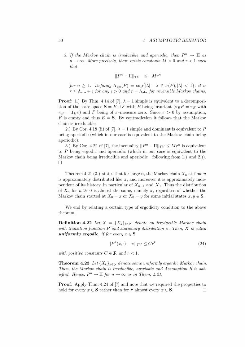
50 4 ASYMPTOTIC BEHAVIOR
3. If the Markov chain is irreducible and aperiodic, then Pn → Π asn→∞. More precisely, there exists constants M > 0 and r < 1 suchthat
||Pn −Π||TV ≤ Mrn
for n ≥ 1. Defining Λabs(P ) = sup|λ| : λ ∈ σ(P ), |λ| < 1, it isr ≤ Λabs + ǫ for any ǫ > 0 and r = Λabs for reversible Markov chains.
Proof: 1.) By Thm. 4.14 of [7], λ = 1 simple is equivalent to a decomposi-tion of the state space S = E ∪ F with E being invariant (πEP = πE withπE = 1Eπ) and F being of π–measure zero. Since π > 0 by assumption,F is empty and thus E = S. By contradiction it follows that the Markovchain is irreducible.
2.) By Cor. 4.18 (ii) of [7], λ = 1 simple and dominant is equivalent to Pbeing aperiodic (which in our case is equivalent to the Markov chain beingaperiodic).
3.) By Cor. 4.22 of [7], the inequality ||Pn −Π||TV ≤Mrn is equivalentto P being ergodic and aperiodic (which in our case is equivalent to theMarkov chain being irreducible and aperiodic—following from 1.) and 2.)).
Theorem 4.21 (3.) states that for large n, the Markov chain Xn at time nis approximately distributed like π, and moreover it is approximately inde-pendent of its history, in particular of Xn−1 and X0. Thus the distributionof Xn for n ≫ 0 is almost the same, namely π, regardless of whether theMarkov chain started at X0 = x or X0 = y for some initial states x, y ∈ S.
We end by relating a certain type of ergodicity condition to the abovetheorem.
Definition 4.22 Let X = Xkk∈N denote an irreducible Markov chainwith transition function P and stationary distribution π. Then, X is calleduniformly ergodic, if for every x ∈ S
||P k(x, ·)− π||TV ≤ Crk (24)
with positive constants C ∈ R and r < 1.
Theorem 4.23 Let Xkk∈N denote some uniformly ergordic Markov chain.Then, the Markov chain is irreducible, aperiodic and Assumption R is sat-isfied. Hence, Pn → Π for n→∞ as in Them. 4.21.
Proof: Apply Thm. 4.24 of [7] and note that we required the properties tohold for every x ∈ S rather than for π almost every x ∈ S.

51
5 Empirical averages
5.1 The strong law of large numbers
Assume that we observe some realization X0(ω),X1(ω), . . . of a Markovchain. Is it possible to “reconstruct” the Markov chain by determiningits transition probabilities just from the observed data?
In general the answer is ’no’; for example, if the Markov chain is re-ducible, we would expect to be able to approximate only the transitionprobabilities corresponding to one communication class. If the Markov chainis transient, the reconstruction attempt will also fail. However, under somereasonable conditions, the answer to our initial question is ’yes’.
In the context of Markov chain theory, a function f : S → R definedon the state space of the chain is called an observable. Observables allowto perform “measurements” on the system that is modelled by the Markovchain. Given some Markov chain Xkk∈N we define the so–called empiri-cal average Sn(f) of the observable f by
Sn(f) =1
n + 1
n∑
k=0
f(Xk).
Note that the empirical average is a random variable, hence Sn(f) : Ω →R ∪ ±∞. Under suitable conditions the empirical average converges to aprobabilistic average, i.e., the expectation valueEπ[f ] =
∑
x∈S
f(x)π(x).
Theorem 5.1 (Strong law of large numbers [2, 17]) Let Xkk∈N de-note an irreducible Markov chain with stationary distribution π, and letf : S→ R be some observable such that
∑
x∈S
|f(x)|π(x) < ∞. (25)
Then for any initial state x ∈ S, i.e., X0 = x
1
n + 1
n∑
k=0
f(Xk) −→ Eπ[f ] (26)
as n→∞ and Px–almost surely, i.e,Px
[
ω : limn→∞
1
n + 1
n∑
k=0
f(
Xk(ω))
= Eπ[f ]
]
= 1.

52 5 EMPIRICAL AVERAGES
Proof: Due to the assumption Xkk∈N is irreducible and positive rekur-rent, therefore ν(y) = Ex[
∑Tx
n=0 1Xn=y] defines an invariant measure, while
the stationary distribution is given by π(y) = ν(y)Z , with the normalization
constant Z =∑
y∈Sν(y) (cp. Theorem 3.19). For the random variable
U0 =∑Tx
k=0 f(Xk) the expectation is given byE[U0] = Ex
[
Tx∑
k=0
f(Xk)
]
= Ex
Tx∑
k=0
∑
y∈S
f(y)1Xk=y
=∑
y∈S
f(y)Ex
[
Tx∑
k=0
1Xk=y
]
=∑
y∈S
f(y)ν(y)
(27)
Now consider Up =∑τp+1
k=τp+1 f(Xk), with p ≥ 1 and Tx = τ0, τ1, τ2, . . . thesuccessive return times to x. It follows from the strong Markov property(Theorem 3.15) that U0, U1, U2, . . . are i.i.d. random variables. Since from(25) and (27) we have E[|U0|] < ∞, therefore the famous Strong Law ofLarge Numbers for i.i.d. random variables can be applied and yields withprobability one, i.e. almost surely,
limn→∞
1
n + 1
n∑
k=0
Uk =∑
y∈S
f(y)ν(y)⇔ limn→∞
1
n + 1
τn+1∑
k=0
f(Xk) =∑
y∈S
f(y)ν(y).
For the moment assume that f ≥ 0 and define Nx(n) :=∑n
k=0 1Xk=x, thenumber of visits in x within the first n steps. Due to
τNx(n) ≤ n < τNx(n)+1
and f ≥ 0 it follows that
1
Nx(n)
τNx(n)∑
k=0
f(Xk) ≤1
Nx(n)
n∑
k=0
f(Xk) ≤1
Nx(n)
τNx(n)+1∑
k=0
f(Xk). (28)
Since the Markov chain is recurrent limn→∞ Nx(n) = ∞, so that the ex-tremal terms in (28) converge to
∑
y∈Sf(y)ν(y) and therefore
limn→∞
1
Nx(n)
n∑
k=0
f(Xk) =∑
y∈S
f(y)ν(y) = Z∑
y∈S
f(y)π(y).
Now consider the observable g ≡ 1, which is positive and fulfills condi-tion (25), since Xkk∈N is recurrent. By the equation above we have
limn→∞
1
Nx(n)
n∑
k=0
g(Xk) = limn→∞
n + 1
Nx(n)= Z ⇒ lim
n→∞
Nx(n)
n + 1=
1
Z,

5.1 The strong law of large numbers 53
and finally
limn→∞
1
n + 1
n∑
k=0
f(Xk) = limn→∞
1
Nx(n)
Nx(n)
n + 1
n∑
k=0
f(Xk)
=1
Z
∑
y∈S
f(y)ν(y) =∑
y∈S
f(y)π(y).
For arbitrary f , consider f+ = max(0, f) and f− = max(0,−f) and takethe difference between the obtained limits.
Theorem 5.1 is often referred to as ergodic theorem. It states that thetime average (left hand side of (26)) is equal to the space average (righthand side of (26)). The practical relevance of the strong law of large num-bers is the following. Assume we want to calculate the expectation Eπ[f ]of some observable f w.r.t. the stationary distribution of the Markov chainXkk∈N. Instead of first computing π and then Eπ[f ], we can alternativelycompute some realization X0(ω),X1(ω), . . . and then determine the corre-sponding empirical average Sn(f). By Theorem 5.1, Sn(f) will be a goodapproximation to Eπ[f ] for “large enough” n and almost every realizationω ∈ Ω.
Why should we do so? There are many applications, for which the transi-tion matrix of the Markov chain is not given explicitly. Instead, the Markovchain is specified by an algorithm of how to compute a realization of it (thisis, e.g., the case, if the Markov chain is specified as a stochastic dynamicssystem like in eq. (5)) . In such situations, the strong law of large numberscan be extremely useful. Of course, we have to further investigate the ap-proximation quality of the expectation by empirical averages, in particulartry to specify how large “large enough” is.
Example 5.2 Consider as observable f : S → R the indicator function ofsome subset A ⊂ S, i.e.,
f(x) = 1x ∈ A =
1; if x ∈ A
0; otherwise .
Then under the conditions of Theorem 5.1
1
n + 1
n∑
k=0
1Xk ∈ A =1
n + 1
n∑
k=0
1A(Xk) −→ π(A)
as n→∞. Hence, π(A) can be interpreted as the long time average numberof visits to the subset A. Consequently for large enough n, π(A) approx-imately denotes the probability of encountering the Markov chain after nsteps in subset A.

54 5 EMPIRICAL AVERAGES
Remark. In our introductory example (random surfer on the WWW)we considered the transition matrix P = (pw,w′)w,w′=1,...,N with
pw,w′ = P[wj+1 = w′|wj = w]
according to (1). The associated chain is irreducible, and aperiodic on finitestate space. Its stationary distribution π thus is unique, positive everywhereand given by either πP = π. The probability pw of a visit of the averagesurfer on webpage w ∈ 1, . . . , N is the relative frequency of visits in win some infinitely long realization of the chain. It is given by its stationarydistribution
pw = limn→∞
1
n + 1
n∑
j=0
1wj = w = π(w).
Thus the ranking of webpage can be computed by solving the eigenvalueproblem πP = π, which is very large since the number N of webpages in theWWW is extemely large (N is in the range of 1010). Thus direct numericalsolution of the eigenvalue problem is prohibitive, and only iterative solverscan lead to success. Google’s famous page rank algorithm is an iterativescheme for computing the solution π iteratively via the application of thepower method to πP = π.
To answer the initial question whether we can reconstruct the transitionprobabilities from a realization, we state the following
Corollary 5.3 (Strong law of large numbers II [2]) Let Xkk∈N de-note an irreducible Markov chain with transition matrix P =
(
P (x, y))
x,y∈S
and stationary distribution π, and let g : S× S→ R be some function suchthat
∑
x,y∈S
|g(x, y)|π(x)P (x, y) < ∞.
Then for any initial state x ∈ S, i.e., X0 = x we have
1
n + 1
n∑
k=0
g(Xk,Xk+1) −→ Eπ,P [g] =∑
x,y∈S
g(x, y)π(x)P (x, y)
as n→∞ and Px–almost surely.
Proof: We leave this as an excercise. Prove that π(x)P (x, y) is a stationarydistribution of the bivariate Markov chain Yk = (Xk,Xk+1).
Corollary 5.3 is quite useful for our purpose. Consider the functiong : S× S→ R with
g(x, y) = 1(u,v)(x, y) =
1; if x = u, y = v
0; otherwise .
5.2 Central limit theorem 55
Under the condition of Corollary 5.3
1
n + 1
n∑
k=0
1Xk = u,Xk+1 = v −→ π(u)P (u, v)
as n → ∞. Hence, if we first compute π(u) as outlined in Example 5.2with A = u, we can then approximate the transition probability P (u, v)by computing the average number of “transitions Xk = u,Xk+1 = v” with0 ≤ k < n and divide it by nπ(u).
5.2 Central limit theorem
We are now ready to state the important central limit theorem:
Theorem 5.4 (central limit theorem) Let Xkk∈N denote an irredu-cible reversible Markov chain with stationary distribution π. Let moreoverf : S→ R denote some observable satisfying
∑
x∈S
|f(x)|π(x) < ∞.
Then, for every initial state X0 = x ∈ S:
(i) The variance of the empirical averages satisfies
n Var
[
1
n
n−1∑
k=0
f(Xk)
]
−→ σ2(f)
as n→∞, where σ2(f) is called the asymptotic variance w.r.t. f .
(ii) If σ(f) <∞, then the distribution of the empirical averages satisfies
√n
(
1
n
n−1∑
k=0
f(Xk)−Eπ[f ]
)
−→ N(
0, σ2(f))
(29)
for n→∞, where the convergence is understood in distribution, i.e.,
limn→∞
P [ω :√
n
(
1
n
n−1∑
k=0
f(Xk(ω))−Eπ[f ]
)
≤ z
]
= Φσ(f)(z)
for every z ∈ R. Here Φ : R→ R given by
Φσ(f)(z) =1
√
2πσ2(f)
∫ z
−∞exp
(
− y2
2σ2(f)
)
dy
denotes the distribution function of the normal distribution with meanzero and variance σ2(f).
56 5 EMPIRICAL AVERAGES
Remarks. For P acting onM2(π) define the quantity Λmax(P ) = supλ ∈σ(P ) : λ 6= 1 ≤ 1.
1. The convergence process related to the asymptotic variance can becharacterized more precisely by
Var
[
1
n
n−1∑
k=0
f(Xk)
]
=σ2(f)
n+O
(
1
n2
)
.
2. We have the upper bound on the asymptotic variance in terms ofΛmax(P ). If Λmax(P ) < 1, then
σ2(f) ≤ 1 + Λmax(P )
1− Λmax(P )〈f, f〉π <∞.
3. For finite state space case we always have Λmax(P ) < 1.
4. The asymptotic variance in the central limit theorem is related to theconvergence rates of the empirical averages Sn(f). The smaller theasymptotic variance σ2(f), the better the convergence of Sn(f) to itslimit values Eπ[f ].
5. Equation (29) is often interpreted in the following way to quantifyconvergence for a given observable f . For large n we approximatelyhave
(
1
n
n−1∑
k=0
f(Xk)−Eπ[f ]
)
≈ 1√nN(
0, σ2(f))
in a distributional sense. Hence if we quadruple the length of theMarkov chain realization, we gain only the double precision.
6. Note that the asymptotic variance depends on the observable f . Hence,for one and the same Markov chain the asymptotic variance may besmall for one observable, but large for another.
5.3 Markov Chain Monte Carlo
We will now give a very short summary of the idea behind Markov ChainMonte Carlo (MCMC). There are many different (and very general) ap-proaches to the construction of MCMC methods; however, we will concen-trate completely on Metropolis MCMC.

5.3 Markov Chain Monte Carlo 57
The background. We consider the following problem: Let π be a prob-ability distribution on state space S. We are interested in computing theexpectation value of some observable f : S→ R,Eπ[f ] =
∑
x∈S
f(x)π(x).
For the sake of simplification we consider π and f to be everywhere positiveboth. If the state space is gigantic the actual computation of the expectationvalue may be a very hard or even seemingly infeasible task. Furthermore, inmany such applications the value of π(x) for some arbitrary x ∈ S cannotbe computed explicitly but has the form
π(x) =1
Zµ(x),
with some µ for which µ(x) is explicitly given and easily computable butthe normalization constant
Z = Eπ[1] =∑
x∈S
π(x),
is not!
The idea. Given π we want to construct an irreducible Markov ChainXkk∈N such that
(C1) π is a stationary distribution of Xkk∈N, and
(C2) realizations of Xkk∈N can be computed by evaluations of µ only(without having to compute Z).
Then we can exploit the law of large numbers and approximate the desiredexpectation value by mean values Sn(f) of finite realization of Xkk∈N:
Sn(f) =1
n + 1
n∑
k=0
f(Xk) −→ Eπ[f ].
Theory. We start with the assumption that we have a transition functionQ : S × S → R that belongs to an irreducible Markov Chain. We can takeany irreducible transition function; it does not need to have any relation toπ but should have the additional property of being efficiently computable.Surprisingly this is enough to construct an irreducible Markov chain withabove properties (C1) and (C2):

58 5 EMPIRICAL AVERAGES
Theorem 5.5 Let π > 0 be the given probability distribution and Q : S ×S→ R a transition function of an arbitrary irreducible Markov Chain whichsatisfies
Q(x, y) 6= 0 ⇔ Q(y, x) 6= 0,
which we will call the proposal function. Furthermore let Ψ : (0,∞)→ (0, 1]be a function satisfying
Ψ(x)
Ψ(1/x)= x, for all x ∈ (0,∞).
Then, the acceptance function A : S× S→ (0, 1] is defined by
A(x, y) =
Ψ(
π(y)Q(y,x)π(x)Q(x,y)
)
∈ (0, 1] if Q(x, y) 6= 0
0 otherwise,
and the transition function P : S× S→ R by
P (x, y) =
Q(x, y)A(x, y) if x 6= y1− ∑
z∈S,z 6=x
Q(x, z)A(x, z) if x = y . (30)
Then the Markov Chain Xkk∈N associated with P is irreducible, and hasπ as stationary distribution, i.e., πP = π.
Proof: First, we observe that P indeed is a transition function:
∑
y∈S
P (x, y) =∑
z∈S,z 6=x
Q(x, z)A(x, z) + 1−∑
z∈S,z 6=x
Q(x, z)A(x, z) = 1.
Furthermore, since π > 0 and Q ≥ 0 per definition, we have A ≥ 0 andP ≥ 0, and in particular A > 0 and P > 0 whenever Q > 0. Thus P inheritsthe irreducibility from Q.
Next, assume that x, y ∈ S are chosen such that Q(x, y) 6= 0 and there-fore Q(y, x) 6= 0; then also P (x, y) > 0 and therefore P (y, x) > 0, and thesame for A. Hence, we compute by exploitation of the property of Ψ:
A(x, y)
A(y, x)=
π(y)Q(y, x)
π(x)Q(x, y),
and therefore finally
π(x)P (x, y) = π(y)P (y, x). (31)
The same equation is obviously satisfied if x = y. If x 6= y and such thatQ(x, y) = 0 then also P (x, y) = 0 such that (31) is satisfied again. Thus,the detailed balance condition (31) is valid for all x, y ∈ S. Then, by Theo-rem 4.13, π is a stationary distribution of Xkk∈N and πP = π.

5.3 Markov Chain Monte Carlo 59
The usual choice for the function Ψ is the so-called Metropolis function
Ψ(x) = min1, x.
In contrast to this, the transition function Q needs to be chosen individuallyfor each application under consideration.
Algorithmic realization. Computing a realization (xk)k=0,1,2,... of theMarkov Chain Xkk∈N associated with the transition function P is easierthan expected:
1. Start in some state x0 with iteration index k = 0.
2. Let xk be the present state.
3. Draw y from the proposal distribution Q(xk, ·). This can be done asdescribed in Sec. 2.3.
4. Compute the acceptance probability
a = A(xk, y) = Ψ( π(y)Q(y, xk)
π(xk)Q(xk, y)
)
= Ψ( µ(y)Q(y, xk)
µ(xk)Q(xk, y)
)
.
5. Draw r ∈ [0, 1) randomly from a uniform distribution in [0, 1).
6. Set
xk+1 =
y if r ≤ axk if r > a
.
7. Set k := k + 1 and return to step 2.
Thus, a = A(xk, y) really is an acceptance probability since the proposedstate y is taken as the next state xk+1 with probability a, while we remainin the present state (xk = xk+1) with probability 1− a.
If in addition Q is symmetric, i.e., Q(x, y) = Q(y, x) for all pairs x, y ∈ S,then the acceptance probability takes the particularly simple form
A(xk, y) = Ψ( µ(y)
µ(xk)
)
.
General remarks. We observe that we do not need the normalizationconstant Z from π = µ/Z; instead we only need fractions of the formµ(x)/µ(y). Thus, we achieved everything we wanted, and we can computethe desired expectation values from the mean values Sn(f) of realization ofXkk∈N. The speed of convergence Sn(f) → Eπ[f ] is given by the cen-tral limit theorem; we can apply Theorem 5.4 since the chain Xkk∈N isreversible by construction. From our remarks to the central limit theoremon page 56 we learn that the variance of the random variables Sn(f) will
60 5 EMPIRICAL AVERAGES
decay with O(n−1σ2(f)) with an asymptotic variance σ2(f) that essentiallydepends on largest eigenvalues of P (not counting λ = 1). It is an art tochoose Q in a way that minimizes these largest eigenvalues of P and thusminimizes the asymptotic variance.

61
6 Markov jump processes
In the following two sections we will consider Markov processes on discretestate space but continuous in time. Many of the basic notions and definitionsfor discrete-time Markov chains will be repeated. We do this without toomuch reference to the former sections in order to make the following sectionsreadable on their own.
6.1 Setting the scene
Consider some probability space (Ω,A,P), where Ω is called the samplespace, A the set of all possible events (the σ–algebra) and P is some prob-ability measure on Ω. A family X = X(t) : t ≥ 0 of random variablesX(t) : Ω → S is called a continuous-time stochastic process on thestate space S. The index t admits the convenient interpretation as time:if X(t) = y, the process is said to be in state y at time t. For some givenω ∈ Ω, the S–valued set X(t, ω) : t ≥ 0 is called a realization (trajectory,sample path) of the stochastic process X associated with ω.
Definition 6.1 (Markov process) A continuous-time stochastic processX(t) : t ≥ 0 on a countable state space S is called a Markov process, iffor any tk+1 > tk > . . . > t0 and B ⊂ S the Markov propertyP[X(tk+1) ∈ B|X(tk), . . . ,X(t0)] = P[X(tk+1) ∈ B|X(tk)] (32)
holds. If, moreover, the right hand side of (32) does only depend on thetime increment tk+1 − tk, but not on tk, then the Markov process is calledhomogeneous. Given a homogeneous Markov process, the function p :R+ × S× S→ R+ defined by
p(t, x, y) = P[X(t) = y|X(0) = x]
is called the stochastic transition function; its values p(t, y, z) are the(conditional) transition probabilities to move from x to y within time t. Theprobability distribution µ0 satisfying
µ0(x) = P[X(0) = x]
is called the initial distribution. If there is a single x ∈ S such thatµ0(x) = 1, then x is called the initial state.
In the following, we will focus on homogeneous Markov process, and thus theterm Markov process will always refer to a homogeneous Markov process,unless otherwise stated.
There are some subtleties in the realm of continuous time processes thatare not present in the discrete-time case. These steam from the fact that the

62 6 MARKOV JUMP PROCESSES
uncountable union of measurable sets need not be measurable anymore. Forexample, the mapping X(t, ·) : Ω → S is measurable for every t ∈ R+, i.e.,ω ∈ Ω : X(t, ω) ∈ A ∈ A for every measurable subset A ⊂ S. However,
ω ∈ Ω : X(t, ω) ∈ A, t ∈ R+ =⋂
t∈R+
ω ∈ Ω : X(t, ω) ∈ A
need not be in A in general. This is related to functions like inft∈R+ X(t)or supt∈R+ X(t), since, e.g.,
supt∈R+
X(t) ≤ x
=⋂
t∈R+
ω ∈ Ω : X(t, ω) ≤ x.
We will therefore impose some (quite natural) regularity conditions onthe Markov process in order to exclude pathological cases (or too technicaldetails). Throughout this chapter, we assume that
p(0, x, y) = δxy, (33)
where δxy = 1, if x = y and zero otherwise. This guarantees that no transi-tion can take place at zero time. Moreover, we assume that the transitionprobabilities are continuous at t = 0:
limt→0+
p(t, x, y) = δxy (34)
for every x, y ∈ S. This guarantees (up to stochastic equivalence) that therealizations of X(t) : t ≥ 0 are right continuous functions (more precisely,it implies that the Markov process is stochastically continuous, separable andmeasurable on compact intervals. Moreover, there exists a separable version,being stochastically equivalent to X(t) : t ≥ 0 and all of whose realizationsare continuous from the right; for details see reference [18, Chapt. 8.5]). Dueto the fact that the state space is discrete, continuity from the right of thesampling functions implies that they are step functions, that is, for almostall ω ∈ Ω and all t ≥ 0 there exists ∆t(t, ω) > 0 such that
X(t + τ, ω) = X(t, ω); τ ∈ [0,∆t(t, ω)).
This fact motivates the name Markov jump process.
For our further study, we recall to important random variables. A con-tinuous random variable τ : Ω→ R+ satisfyingP[τ > s] = exp(−λs)
for every s ≥ 0 is called an exponential random variable with parameterλ ≥ 0. Its probability density f : R+ → R+ is given by
f(s) = λ exp(−λs)

6.1 Setting the scene 63
for s ≥ 0 (and zero otherwise). Moreover, the expectation is given byE[τ ] =1
λ.
One of the most striking features of exponential random variables is theirmemoryless property, expressed asP[τ > t + s|τ > t] = P[τ > s]
for all s, t ≥ 0. This is easily proven by noticing that the left hand side isper definition equal to exp(−λ(t + s))/ exp(−λt) = exp(−λs), being equalto the right hand side.
A discrete random variable N : Ω→ N with probability distributionP[N = k] =λke−λ
k!
for k ∈ N is called a Poisson random variable with parameter λ ∈ R+.Its expectation is given by E[N ] = λ.
We now consider two examples of Markov jump processes that are of proto-type nature.
Example 6.2 Consider an iid. sequence τkk∈N of exponential randomvariable with parameter λ > 0 and define recursively the sequence of randomvariable Tkk∈N by
Tk+1 = Tk + τk
for k ≥ 1 and T0 = 0. Here, Tk is called the kth event time and τk theinter-event time. Then, the sequence of random variables N(t) : t ≥ 0defined by
N(t) =
∞∑
k=0
1Tk≤t = max k ≥ 0 : Tk ≤ t .
for t ≥ 0 and with N(0) = 0. Its (discrete) distribution is given by thePoisson distribution with parameter λt:P[N(t) = k] =
(λt)k
k!e−λt;
for k ≥ 1. That is why N(t) is called a homogeneous Poisson process
with intensity λ. Per construction, N(t) is counting the number of eventsup to time t. Therefore, it is also sometime called the counting process
associated with Tk.

64 6 MARKOV JUMP PROCESSES
Remark: One could also determine the distribution of the event timesTk, the time at which the kth event happens to occur. Since per definitionTk is the sum of k iid. exponential random variables with parameter λ, theprobability density is known as
fTk(t) =
(λt)k
k!λe−λt
for t ≥ 0 and zero otherwise. This is the so-called Erlang distribution (aspecial type of Gamma distribution) with parameter k + 1 and λ.
Example 6.3 Consider some discrete-time Markov chain Ekk∈N on acountable state space S with stochastic transition matrix K = (k(x, y))xy∈S,and furthermore, consider some homogeneous Poisson process Tkk∈N onR+ with intensity λ > 0 and associated counting process N(t) : t ≥ 0.Then, assuming independence of Ek and N(t), the process X(t) : t ≥0 with
X(t) = EN(t)
is called the uniform Markov jump process with clock N(t) and sub-ordinated chain Ek. The thus defined process is indeed a Markov jumpprocess (exercise). Note that the jumps of X(t) are events of the clock pro-cess N(t), however, not every event of N(t) corresponds to a jump (unlessE(x, x) = 0 for all x ∈ S). In order to compute its transition probabilities,note thatP[X(t) = y|X(0) = x] = P[EN(t) = y|E0 = x]
=
∞∑
n=0
P[En = y,N(t) = n|E0 = x]
=
∞∑
n=0
P[En = y|E0 = x] P[N(t) = n],
where the last equality is due to the assumed independence of En and N(t).Hence, its transition probabilities are given by
p(t, x, y) =
∞∑
n=0
e−λt (λt)n
n!kn(x, y), (35)
for t ≥ 0, x, y ∈ S, where kn(x, y) is the corresponding entry of Kn, then-step transition matrix of the subordinated Markov chain.
Solely based on the Markov property, we will now deduce some propertiesof Markov jump processes that illuminate the differences, but also the close
6.1 Setting the scene 65
relations to the realm of discrete-time Markov chains. We will see thatthe uniform Markov chain is in some sense the prototype of a Markov jumpprocess. To do so, define for t ∈ R+ the residual life time τ(t) : S→ [0,∞]in state X(t) by
τ(t) = infs > 0 : X(t + s) 6= X(t). (36)
Obviously, τ(t) is a stopping time, i.e., it can be expressed in terms ofX(s) : 0 ≤ s ≤ t (since the sample paths are right-continuous). Hence,conditioned on X(t) and τ(t) <∞, the next jump (state change) will occurat time t+ τ(t). Otherwise the Markov process will not leave the state X(t)anymore.
Proposition 6.4 Consider some Markov process X(t) : t ≥ 0 being instate x ∈ S at time t ∈ R+. Then, there exists λ(x) ≥ 0, independent of thetime t, such that P[τ(t) > s|X(t) = x] = exp(−λ(x)s) (37)
for every s > 0.
Therefore, λ(x) is called the jump rate associated with the state x ∈ S.Prop. 6.4 states that the residual life time decays exponentially in s.
Proof: Note that P[τ(t) > s|X(t) = x] = P[τ(0) > s|X(0) = x], since theMarkov jump process is homogeneous. Define g(s) = P[τ(0) > s|X(0) = x]and compute
g(t + s) = P[τ(0) > t + s|X(0) = x] = P[τ(0) > t, τ(t) > s|X(0) = x]
= P[τ(0) > t|X(0) = x]P[τ(t) > s|τ(0) > t,X(0) = x]
= g(t)P[τ(t) > s|τ(0) > t,X(0) = x,X(t) = x]
= g(t)P[τ(t) > s|X(t) = x] = g(t)g(s).
In addition, g(s) is continuous at s = 0, since the transition probabilitieswere assumed to be continuous at zero. Moreover, 0 ≤ g(s) ≤ 1, whichfinally implies that the only solution must be
g(s) = exp(−λ(x)s)
with λ(x) ∈ [0,∞] given by λ(x) = − ln(P[τ(0) > 1|X(0) = x]).
To further illuminate the characteristics of Markov processes on count-able state spaces, denote by T0 = 0 < T1 < T2 < . . . the random jumptimes or event times, at which the Markov process changes its state. Based

66 6 MARKOV JUMP PROCESSES
on the jump times, define the sequence of random life times (τk)k∈N viathe relation
τk = Tk+1 − Tk
for k ∈ N. Due to Prop. 6.4 we know thatP[τk > s|X(Tk) = x] = exp(−λ(x)s)
for s ≥ 0. Moreover, the average life time of a state isE[τ(t)|X(t) = x] =1
λ(x).
In terms of the jump times, we have
X(t) = X(Tk); t ∈ [Tk, Tk+1),
hence the Markov process is constant, except for the jumps.
Definition 6.5 Consider a state x ∈ S with associated jump rate λ(x).Then, x is called
1. permanent, if λ(x) = 0
2. stable, if 0 < λ(x) <∞,
3. instantaneous, if λ(x) = ∞ (not present for Markov processes withright continuous sample paths).
Assume that X(t) = x at time t; if x is
1. permanent, then P[X(s) = x|X(t) = x] = 1 for every s > t, hence theMarkov process stays in x forever,
2. stable, then P[0 < τ(t) <∞|X(t) = x] = 1,
3. instantaneous, then P[τ(t) = 0|X(t) = x] = 1, hence the Markovprocess exists the state as soon as it enters it.
Due to our general assumption, we know that the Markov process has rightcontinuous sample paths. As a consequence, the state space S does notcontain instantaneous states.
Definition 6.6 Consider some Markov process X(t) : t ≥ 0 with rightcontinuous sample paths. Then, the Markov process is called regular ornon-explosive, if
T∞ := supk∈NTk =∞ (a.s.),
where T0 < T1 < . . . denote the jump times of X(t) : t ≥ 0. The randomvariable T∞ is called the explosion time.

6.1 Setting the scene 67
If the Markov jump process is explosive, then P[T∞ < ∞] > 0. Hencethere is a ”substantial” set of realizations, for which the Markov process”blows up” in finite time. In such a situation, we assume that the Markovjump process is only defined for times smaller than the explosion time. Thefollowing proposition provides a quite general condition for a Markov processto be regular.
Proposition 6.7 A Markov process X(t) : t ≥ 0 on a countable statespace S is regular, if and only if
∞∑
k=1
1
λ(X(Tk))=∞ (a.s.).
This is particularly the case, if (1) S is finite, or (2) if supx∈S λ(x) <∞.
Proof: See Prop. 8.7.2 in [18].
Compare also Prop. 6.16. Based on the sequence of event times (Tk)k∈N,we define the following discrete-time S-valued stochastic process Ek byEk = X(Tk). As is motivated from the definition and the following results,Ekk∈N is called the embedded Markov chain. However, it still remains toprove that Ekk∈N is really well-defined and Markov. To do so, we needthe following
Definition 6.8 A Markov process X(t) : t ≥ 0 on a state space S fulfillsthe strong Markov property if, for any stopping time τ , being finite a.s.,P[X(s + τ) ∈ A|X(τ) = x,X(t), t < τ ] = Px[X(s) ∈ A]
for every A ∈ A, whenever both sides are well-defined. Hence, the processX(s + τ) : s ≥ 0 is Markov and independent of X(t), t < τ, givenX(τ) = x.
In contrast to the discrete-time case, not every continuous-time Markovprocess on a countable state space obeys the strong Markov property. How-ever, under some suitable regularity conditions, this is true.
Theorem 6.9 A regular Markov process on a countable state space fulfillsthe strong Markov property.
Proof: See Thm. 4.1 in Chapter 8 of [2].
The next proposition states that the time, at which the Markov processjumps next, and the state, it jumps into, are independent.

68 6 MARKOV JUMP PROCESSES
Proposition 6.10 Consider a regular Markov jump process on S, and as-sume that Tk+1 < ∞ a.s. Then, conditioned on X(Tk) = x, the randomvariables τk+1 and X(Tk+1) are independent, i.e.,P[τk+1 > t,X(Tk+1) = y|X(Tk) = x] (38)
= P[τk+1 > t|X(Tk) = x] ·P[X(Tk+1) = y|X(Tk) = x]
Proof: Starting with (38) we get, by applying Bayes rule,P[τk+1 > t,X(Tk+1) = y|X(Tk) = x]
= P[τk+1 > t|X(Tk) = x] ·P[X(Tk+1) = y|X(Tk) = x, τk+1 > t].
Using the Markov property we can rewrite he last factorP[X(Tk+1) = y|X(Tk) = x, τk+1 > t]
= P[X(Tk+1) = y,X(s) = x, Tk ≤ s < Tk+1|X(Tk + t) = x]
= P[X(Tk + τ(Tk + t)) = y,X(s) = x, Tk ≤ s < Tk + τ(Tk + t)|X(Tk) = x]
= P[X(Tk+1) = y|X(Tk) = x],
where we used the homogeneity of the Markov process to proceed from thesecond to the third line.
We are now ready to define the embedded Markov chain of theMarkov jump process.
Definition 6.11 Define the homogeneous Markov chain Ekk∈N on thestate space S in terms of the following transition function P =
(
p(x, y))
xy∈S.
If x is permanent, set p(x, x) = 1. Otherwise, if x is stable, set
p(x, y) = P[X(T1) = y|X(0) = x] (39)
and consequently p(x, x) = 0.
Summarizing our results we obtain the following theorem.
Theorem 6.12 Consider a regular Markov jump process and assume thatthe state space consists only of stable states. Then, X(Tk)k∈N is a ho-mogeneous Markov chain with transition function defined in (39). In otherwords, it is
Ek = X(Tk)
for every k ∈ N (in distribution).
So, we obtain the following characterization of a Markov jump processesX(t) on the state space S. Assume that the process is at state x at timet, i.e., X(t) = x. If the state is permanent, then the Markov process will

6.2 Communication and recurrence 69
stay in x forever, i.e., X(s) = x for all s > t. If the state is stable, then theMarkov process will leave the state x at a (random) time being exponentiallydistributed with parameter 0 < λ(x) < ∞. It then jumps into some otherstate y 6= x ∈ X with probability p(x, y), hence according to the law of theembedded Markov chain Ekk∈N. Therefore knowing the rates (λ(x)) andthe embedded Markov chain in terms of its transition function P = (p(x, y))completely characterizes the Markov jump process.
The above characterization is also the basis for a numerical simulationof the Markov jump process. To do so, one might exploit the followingimportant and well-known relation between an exponential random variableτ with parameter λ and some uniform random variable U on [0, 1], given by
τ = − 1
λln(U).
Hence, a numerical simulation of a Markov jump process can be based onrandomly drawing two uniform random numbers for each jump event (onefor the time, another one for the state change).
6.2 Communication and recurrence
This section is about the topology of regular Markov jump processes (unlessstated otherwise). As in the case of Markov chains, we start with some
Definition 6.13 Let X(t) : t ≥ 0 denote a Markov process with transitionfunction P (t), and let x, y ∈ S denote some arbitrary pair of states.
1. The state x has access to the state y, written x→ y, ifP[X(t) = y|X(0) = x] > 0
for some t > 0.
2. The states x and y communicate, if x has access to y and y accessto x, denoted by x↔ y.
3. The Markov chain is said to be irreducible, if all pairs of states com-municate.
As for Markov chains, it can be proven that the communication relation↔ is an equivalence relation on the state space. We remark that periodicityplays no role for continuous-time Markov jump processes, since they arealways aperiodic. We proceed by introducing the first return time.
Definition 6.14 1. The stopping time Ex : Ω→ R+ ∪ ∞ defined by
Ex = inft ≥ 0 : X(t) 6= x,X(0) = x.is called the first escape time from state x ∈ S.

70 6 MARKOV JUMP PROCESSES
2. The stopping time Rx : Ω→ R+ ∪ ∞ defined by
Rx = inft > T1 : X(t) = x,
with inf =∞, is called the first return time to state x.
Note that Px[Ex] = Px[τ(0)] (see eq. (36)).
Analogous to the Markov chain theory, based on the first return time toa state, we may define recurrence and transience of a state.
Definition 6.15 A state x ∈ S is called recurrent, if it is permanent orPx[Rx =∞] = 1,
and transient otherwise.
Again, recurrence and transience are class properties, i.e., the states of somecommunication class are either all recurrent or all transient. Interestinglyand maybe not surprisingly, some (but not all, as we will see later) propertiesof states can be determined in terms of the embedded Markov chain.
Proposition 6.16 Consider a regular and stable Markov jump process X(t) :t ≥ 0 and the associated embedded Markov chain Ekk∈N, then the fol-lowing holds true.
a) The Markov jump process is irreducible, if and only if its embedded Markovchain is irreducible.
b) A state x ∈ S is recurrent (transient) for the embedded Markov chain, ifand only if is recurrent (transient) for the Markov jump process.
c) A state x ∈ S is recurrent for the Markov jump process, if and only if
∫ ∞
0p(t, x, x)dt =∞.
d) Recurrence and transience of the Markov process inherits to any dis-cretization, i.e. if h > 0 and Zk := X(kh) then recurrence of x ∈ S forthe Markov process is equivalent to recurrence of x ∈ S for the discretiza-tion Zkk∈N.
Proof: We leave the proof of the first two statements as an exercise to thereader.c) Remember the analogous formulation in the time-discrete case: if forsome Markov chain, e.g. Ekk∈N, and some state, e.g. x ∈ S, the random

6.2 Communication and recurrence 71
variable Nx counts the number of visits in x, then x is recurrent if and onlyif Ex[Nx] = Ex
[
∞∑
k=0
1Ek=x
]
=
∞∑
k=0
Ex[1Ek=x]
=
∞∑
k=0
p(k)(x, x) =∞,
where, as usual, p(k)(x, x) denotes the k−step transition probabilityPx[Ek =x]. Therefore we can prove the statement by showing that
∫ ∞
0p(t, x, x)dt =
1
λ(x)
∞∑
k=0
p(k)(x, x).
This is done in the following, where we use Fubini’s theorem to exchangeintegral and expectation and Beppo Levi’s theorem to exchange summationand expectation:∫ ∞
0p(t, x, x)dt =
∫ ∞
0Ex[1X(t)=x]dt = Ex
[∫ ∞
01X(t)=xdt
]
= Ex
[
∞∑
k=0
τk+11Ek=x
]
=
∞∑
k=0
Ex[τk+1|Ek = x]Px[Ek = x]
=
∞∑
k=0
1
λ(x)p(k)(x, x)
Be aware that the conditions to use Fubini’s theorem are only met becauseX is a jump process.d) That transience inherits to any discretization is obvious, so consider xrecurrent. If t is constrained by kh ≤ t < (k + 1)h, then
p((k + 1)h, x, x) ≥ p((k + 1)h− t, x, x)p(t, x, x)
≥ exp(−λ(x)((k + 1)h− t)p(t, x, x)
≥ exp(−λ(x)h)p(t, x, x).
Multiplication with exp(λ(x)h) yields
exp(λ(x)h)p((k + 1)h, x, x) ≥ p(t, x, x) , for kh ≤ t < (k + 1)h.
This enables us to give an upperbound to the integral
∫ ∞
0p(t, x, x)dt ≤ h
∞∑
k=0
exp(−λ(x)h)p((k + 1)h, x, x)
= h exp(−λ(x)h)∞∑
k=1
p(kh, x, x).
72 6 MARKOV JUMP PROCESSES
It follows from d) that∑∞
k=1 p(kh, x, x) = ∞, which is the sum over thetransition probabilities of the discretized Markov chain.
Irreducible and recurrent Markov jump processes are regular, as the nexttheorem states.
Theorem 6.17 An irreducible and recurrent Markov jump process is regu-lar.
Proof: Regularity means that the sequence of event times heads to infinity
limk→∞
Tk =∞⇔∞∑
k=1
τk =∞.
Let x ∈ S be an arbitrary start position. Since the Markov process is irre-ducible and recurrent, we know that the embedded Markov chain Ekk∈Nvisits x infinitely often. Denote by Nk(x)k∈N the sequence of visits in x.Observe that if τ is λ−exponential distributed, then λτ is 1−exponentialdistributed (we pose that as an easy exercise), therefore we have
∞ =
∞∑
k=0
λ(ENk(x))τNk+1 = λ(x)
∞∑
k=0
τNk+1
≤ λ(x)∞∑
k=0
τk+1.
As we will see below, it is also possible to characterize invariant measuresin terms of the embedded Markov chain. However, the distinction betweenpositive and null-recurrence and the existence of stationary distributions cannot be examined in terms of the embedded Markov chain. Here, the rates(λ(x)) also have to come into play. That is why we postpone the correspond-ing analysis and first introduce the concept of infinitesimal generators, whichis the more adequate object to study.
6.3 Infinitesimal generators and the master equation
We now come to the characterization of Markov jump processes that is notpresent for the discrete-time case. It is in terms of infinitesimal changes ofthe transition probabilities and based on the notion of generators. As inthe preceding section, we assume throughout that the Markov jump processsatisfies the two regularity conditions (33) and (34).

6.3 Infinitesimal generators and the master equation 73
To start with, we introduce the transition semigroup P (t) : t ≥ 0with
P (t) =(
p(t, x, y))
xy∈S.
Due to (33), it is P (0) = Id and due to (34), we have
limt→0+
P (t) = Id.
In terms of the transition semigroup, we can also easily express the Chapman-Kolmogorov equation as
P (s + t) = P (s)P (t)
for t, s ≥ 0 (which justifies the notion of a semigroup). In semigroup theory,one aims at characterizing P (t) in terms of its infinitesimal generator Q. Inbroad terms, the goal is to prove and justify the notion P (t) = exp(tQ). Inthe following, we will proceed towards this goal.
Proposition 6.18 Consider the semigroup P (t) of a Markov jump process.Then, the limit
A = limt→0+
P (t)− Id
t
exists (entrywise) and defines the infinitesimal generator A = (a(x, y))xy∈S
with −∞ ≤ a(x, x) ≤ 0 ≤ a(x, y) <∞.
Note that we do not claim uniform convergence for all pairs of statesx, y ∈ S.
Proof : We first prove the result for the diagonal entries. Consider somestate x ∈ S and define h(t, x) = − ln(p(t, x, x)). Then, from the Chapman-Kolmogorov equation we deduce p(t + s, x, x) ≥ p(t, x, x)p(s, x, x). In termsof h, this implies h(t + s, x) ≤ h(t, x)h(s, x). Due to the general regularitycondition (33), it is h(0, x) = 0, implying h(t, x) ≥ 0 for all t ≥ 0. Now,define
sup0≤t≤∞
h(t, x)
t=: c ∈ [0,∞].
We now proof that c is in fact equal to the limit limh(t, x)/t for t → +,being equivalent to the statement that for every b < c it is
b ≤ lim inft→0+
h(t, x)
t≤ lim sup
t→0+
h(t, x)
t= c. (40)
So, choose b < c arbitrarily. Acc. to the definition of c, there exists s > 0such that b < h(s, x, x)/s. Rewriting s = nt+∆t with t > 0 and 0 ≤ ∆t < t,we obtain
b <h(s, x)
s≤ nt
s
h(t, x)
t+
h(∆t, x)
s

74 6 MARKOV JUMP PROCESSES
Taking the joint limit t → 0+, ∆t → 0 and n → ∞ such that nt/s →1 proves the first inequality in (40) and thus completes the proof for thediagonal entries.
To prove the statement for the off-diagonal entries, assume that we areable to prove for every ǫ ∈ (1/2, 1) there exist δ > 0 such that
p(ns, x, y) ≥ (2ǫ− 1)np(s, x, y) (41)
for every n ∈ N and s ≥ 0 such that 0 ≤ ns < δ. Denote by [x] the integerpart of x. Then,
p(s, x, y)
s≤ p([t/s]s, x, y)
[t/s]s(2ǫ2 − ǫ)
with t, s < δ. Considering s→ 0+, we obtain for all t > 0
lim sups→0+
p(s, x, y)
s≤ p(t, x, y)
t(2ǫ2 − ǫ)<∞
since lims→0+[t/s]s = t. Therefore,
lim sups→0+
p(s, x, y)
s≤ 1
(2ǫ2 − ǫ)lim inft→0+
p(t, x, y)
t<∞.
Since ǫ can be chosen arbitrarily close to 1, we finally obtain the desiredresult. However, statement (41) still needs to be proven ...
Sometimes, even for discrete-time Markov chains ”generators” are de-fined; here A = P − Id mimics the properties of a infinitesimal generator(which it of course not is). In Graph Theory, such a matrix is known asLaplace matrix.
Example 6.19 Rewriting eq. (35) in matrix form, we obtain for the tran-sition semigroup of the uniform Markov process with intensity λ > 0 andsubordinated Markov chain K = (k(x, y))
P (t) =
∞∑
n=0
e−λt (λt)n
n!Kn = etλ
(
K−Id)
, (42)
for t ≥ 0.The infinitesimal generator is thus given by
A = λ(
K − Id)
, (43)
which, entry-wise, corresponds to a(x, x) = λ(1 − k(x, x)), and a(x, y) =λk(x, y) for x 6= y. The result directly follows from eq. (42).
By now we have two different descriptions of a Markov jump process,one in of form sojourn times and the embedded Markov chain, the other

6.3 Infinitesimal generators and the master equation 75
by the generator. We saw in the preceding sections that a Markov jumpprocess is fully determined by its sojourn times and the embedded Markovchain. Why did we introduce the notion of a generator then? The answer isthat more general Markov processes, i.e. in continuous state space, can notdescribed by an embedded Markov chain anymore, while it is still possibleto use the generator concept. But of course, in the case of a Markov jumpprocess, it is possible to convey both description types into each other, likewe did in the case of a uniform Markov jump process. This is what we doin the next paragraph. Therefore we will construct for a given generator asuitable Markov jump process and use this construction afterwards to getinsight about the entries of a generator of a given Markov jump process.As preparation we need
Proposition 6.20 Consider a series of independent exponential distributedrandom variables Nkk∈N with parameters λkk∈N. Assume that
∑∞k=0 λk =
λ <∞ and letT = minN0, N1, N2, . . . ,
be the minimum value of the random variables series and J such that NJ =T . Then J and T are independent random variables withP[J = i, T ≥ t] = P[J = i]P[T ≥ t] =
λi
λexp(−λt).
Proof : Left as an exercise (use results about the distribution of a mini-mum of exponential distributed random variables, show the proposition fora finite number of random variables and then generalize to the case of aninfinite number of random variables).
Given a stable and conservative generator, i.e. a matrix A with
−∞ < −a(x, x) ≤ 0,
0 ≤ a(x, y) <∞ for x 6= y
and∑
y 6=x a(x, y) = −a(x, x). To construct a jump process based on thismatrix set T0 = 0, X(T0) = X(0) = x0 and define recursively the followingprocess
1. Assume X(Tk) = x.
2. If a(x, x) = 0 end the construction by setting τk = ∞ and X(t) = xfor all t ≥ Tk.
3. Otherwise τk = minNx,0, Nx,1, . . . , Nx,x−1, Nx,x+1, Nx,x+2, . . ., whereN(x, y) is exponential distributed to the parameter a(x, y).
4. Set Tk+1 = Tk + τk and Xk+1 = X(Tk+1) = y, where y is the statesuch that τk = N(x, y).

76 6 MARKOV JUMP PROCESSES
Theorem 6.21 The previous constructed process is a homogeneous Markovjump process with generator A
Proof : We leave the fact that the constructed process is a homogeneousMarkov jump process to the careful reasoning of the reader. It remains toshow that a(x, y) = limt→0
P (t,x,y)−P (0,x,y)t , i.e. it is necessary to analyze
the transition function P . The statement is trivial if a(x, x) = 0 (why?),therefore it is assumed in the following that a(x, x) 6= 0.The first case to be considered is x 6= y, then
P (t, x, y) = Px[T2 ≤ t,X(t) = y] +Px[T2 > t,X(t) = y]
= Px[T2 ≤ t,X(t) = y] +Px[T2 > t, T1 ≤ t,X1 = y]
= Px[T2 ≤ t,X(t) = y] +Px[T1 ≤ t,X1 = y]−Px[T1 ≤ t,X1 = y, T2 ≤ t]
The three terms on the right-hand side are now to be analyzed separately.For the second term we have, by 6.20,Px[T1 ≤ t,X1 = y] = (1− exp(−a(x, x)t)
a(x, y)
a(x, x)=: f(t).
Since f ′(t) = a(x, y) exp(a(x, x)t) we have f ′(0) = a(x, y) and
limt→0
f(t)− f(0)
t= lim
t→0
f(t)
t= a(x, y).
The first and the third term are both upper-bounded by Px[T2 ≤ t], whichcan be bounded further byPx[T2 ≤ t] ≤ Px[T1 ≤ t, τ1 ≤ t]
=∑
x 6=y
Px[T1 ≤ t,X1 = y, τ1 ≤ t]
=∑
x 6=y
(1− exp(a(x, x)t))a(x, x)
−a(x, y)(1− exp(a(y, y)t)) = f(t)g(t),
where f(t) := exp(a(y, y)t) − 1 and g(t) :=∑
x 6=y(1 − exp(a(x, x)t)a(x,x)a(x,y) .
Now observe
limt→0
1
tf(t) = lim
t→0
exp(a(y, y)t) − exp(a(y, y)0)
t− 0= (exp(a(y, y)t))′|t=0 = a(y, y)
and
limt→0
g(t) = limt→0
∑
x 6=y
(1− exp(a(x, x)t)a(x, x)
a(x, y)= 0,
(the exchange of limes and summation is allowed in this case, because allsummands in the sum are positive, bounded and with an existing limes).
This yields limt→0Px[T2≤t]
t = limt→0f(t)g(t)
t = 0 and, putting it all together,
limt→0
P (t, x, y)
t= a(x, y).
6.3 Infinitesimal generators and the master equation 77
It remains to show that limt→0P (t,x,x)−1
t = −a(x, x). This is very similar tothe case x 6= y, in that P (t, x, x) is decomposed by
P (t, x, x) = Px[T2 ≤ t,X(t) = x] +Px[T2 > t,X(t) = x]
= Px[T2 ≤ t,X(t) = x] +Px[T1 > t],
which can be treated similar to the first case to show the assertion.
As it is clear by now how to construct a Markov jump process to a givengenerator we proceed to the reverse direction. Assume a given Markov jumpprocess X(t) : t ≥ 0 with jump rates λ(x)x∈S and conditional transitionprobabilities k(x, y)x,y∈S, furthermore k(x, x) = 0 and λ(x) < ∞ for allx ∈ S. Let P be the transition function of this process. A matrix A definedby
a(x, y) =
−λ(x) for x = y
λ(x)k(x, y) for x 6= y
fulfills obviously the conditions we posed on a generator, namely conserva-tive and stable, to construct a Markov Process by the previous describedprocedure. Doing this we obtain another Markov Process with transitionfunction P . By construction it is clear that P = P (you should be able tofigure that out!) and therefore the derivatives at 0 are equal, that is thegenerator of X(t) : t ≥ 0 fulfills A = A. We state this important result in
Theorem 6.22 Consider a homogeneous and regular Markov jump processon state space S with jump rates λ(x)x∈S and conditional transition prob-abilities k(x, y)x,y∈S, where k(x, x) = 0 for all x ∈ S. Then the generatorA is given by
a(x, y) =
−λ(x) for x = y
λ(x)k(x, y) for x 6= y,
i.e. A = Λ(K − Id), where the jump rate matrix Λ is given by
Λ =
λ(0)λ(1)
λ(2). . .
. (44)
Hence, the negative diagonal entry of the generator corresponds to thelife time rate of the corresponding state, while the off-diagonal entries areproportional to the transition probabilities of the embedded Markov chain.We further remark that many infinitesimal generators can be represent inmultiple ways, if represented by an intensity λ ∈ R+ and some subordinatedMarkov chain with transition matrix S. Assume supx λ(x) <∞. Then, forany choice of λ ≥ supx λ(x), define
S = λ−1Λ(K − Id) + Id,

78 6 MARKOV JUMP PROCESSES
which indeed is a stochastic matrix (exercise). As a result, eq. (43) trans-forms into the uniform representation
A = λ(S − Id), (45)
which is the representation of the infinitesimal generator of an uniformMarkov jump process with intensity λ and subordinated Markov chain rep-resented by S. In the representation (45), every event is associated with astate change (since p(x, x) = 0). In contrast, events in the representation(45) need not necessarily correspond to a state change (since s(x, x) ≥ 0,which might be positive).
Example 6.23 A birth and death process with birth rates (αx)x∈S anddeath rates (γx)x∈S on the state space S = N is a continuous-time Markovjump process with infinitesimal generator A = (a(x, y))xy∈S defined by
A =
−α0 α0 0 0 0 · · ·γ1 −(γ1 + α1) α1 0 0 · · ·0 γ2 −(γ2 + α2) α2 0 · · ·0 0 γ3 −(γ3 + α3) α3 · · ·...
......
. . .. . .
. . .
.
We assume that α(x), γ(x) ∈ (0,∞) for x ∈ S. The birth and death processis regular, if and only if the corresponding Reuters’s criterion
∞∑
k=1
(
1
αk+
γk
αkαk−1+ · · ·+ γk · · · γ1
αk · · ·α0
)
=∞
is satisfied [2, Chapt. 8, Thm. 4.5].
The next proposition shows how the generator can be used to evolve thesemigroup of conditional transitions in time.
Proposition 6.24 Consider a Markov jump process with transition semi-group P (t) and infinitesimal generator A = (a(x, y)), satisfying −a(x, x) <∞ for all x ∈ S. Then, P (t) is differentiable for all t ≥ 0 and satisfies theKolmogorov backward equation
dP (t)
dt= AP (t). (46)
If furthermore∑
y
p(t, x, y)λ(y) <∞ (47)
is satisfied for all t ≥ 0 and x ∈ S, then also the Kolmogorov forward
equationdP (t)
dt= P (t)A (48)
holds.

6.3 Infinitesimal generators and the master equation 79
Remark 6.25 Condition (47) is always satisfied if the state space S is finiteor supx λ(x) <∞.
Proof : There is simple proof in the case of a finite state space. In thegeneral case the proof is considerably harder, we refere to [18], Prop. 8.3.4,p.210.By definition of a semigroup we have P (t + s) = P (t)P (s) = P (s + t),therefore, under the assumption that S is finite,
limh→0
P (t + h)− P (t)
h= lim
h→0P (t)
P (h) − Id
h= P (t)A
= limh→0
P (h)− Id
hP (t) = AP (t)
This does not work in the infinite case, because it is not sure if we can ex-change the limes with the sum in the matrix-matrix multiplication.
Remark 6.26 Component wise the backward, resp. forward, equation reads
d
dtP (t, x, y) = −λ(x)P (t, x, y) +
∑
z 6=x
a(x, z)P (t, z, y), resp.
d
dtP (t, x, y) = −λ(y)P (t, x, y) +
∑
z 6=x
P (t, x, z)a(z, y)
If the state space is finite the solution to eq. (46) is given by P (t) = exp(tA),where the matrix exponential function is defined via the series
exp(tA) =∑
n∈N (tA)n
n!
which is known to converge. The situation is quite easy if A is diagonalizable,i.e. we have A = V −1DV for a unitary matrix V and a diagonal matrix D.Then An = V −1DnV and
exp(tA) =∑
n∈N (tV −1DV )n
n!= V −1
∑
n∈N (tD)n
n!V
= V −1diag(exp(td1), exp(td2), . . . , exp(tdr))V.
In the non-diagonalizable case the exponential function can still be used fora reasonable approximation by computing only part of the sum.¿From the Kolmogorov forward equation we can easily deduce the evolutionequation for an arbitrary initial distribution µ0 = (µ0(x))x∈S of the Markovjump process. As in the discrete-time case, we have
µ(t) = µ0P (t),
80 6 MARKOV JUMP PROCESSES
with µ(t) = (µ(t, x))x∈S and µ(t, x) = Pµ0 [X(t) = x]. Now, multiplyingthe Kolmogorov forward equation with µ0 from the left, we get the so-calledMaster equation
dµ(t)
dt= µ(t)A
with initial condition µ(0) = µ0. It describes on an infinitesimal scale theevolution of densities w.r.t. the Markov process. An alternative formulationcan be given in terms of the jump rates λ(x) and the embedded Markovchain K = (k(x, y))
dµ(t, z)
dt=
∑
y∈S
µ(t, y)a(y, z)
= λ(z)∑
y∈S
(
µ(t, y)− µ(t, z))
k(y, z)
for every z ∈ S.
6.4 Invariant measures and stationary distributions
This section studies the existence of invariant measures and stationary (prob-ability) distributions. We will see that the embedded Markov chain is stilla very useful object with this regard, but we will also see that not everyproperty of the continuous-time Markov process can be specified in terms ofthe embedded discrete-time Markov chain. This is particularly true for theproperty of positive recurrence.
Definition 6.27 A measure µ = (µ(x))x∈S satisfying
µ = µP (t)
for all t ≥ 0 is called an invariant measure of the Markov jump process.If, moreover, µ is a probability measure satisfying µ(S) = 1, it is called astationary distribution.
We are now able to state for a quite large class of Markov jump processesthe existence of invariant measures, and also to specify them.
Theorem 6.28 Consider an irreducible and recurrent regular Markov jumpprocess on S with transition semigroup P (t). For an arbitrary state x ∈ Sdefine µ = (µ(y))y∈S via
µ(y) = Ex
[∫ Rx
01X(s)=yds
]
, (49)
the expected time, the process visits y before returning to x. Then

6.4 Invariant measures and stationary distributions 81
1. 0 < µ(y) < ∞ for all y ∈ S. Moreover, µ(x) = 1/λ(x) for the statex ∈ S chosen in the eq. (49).
2. µ = µP (t) for all t ≥ 0.
3. If ν = νP (t) for some measure ν, then ν = αµ for some α ∈ R.
Proof: See Bremaud Thm. 5.1, p 357. We just prove here µ(x) = 1/λ(x).We have
µ(x) = Ex
[∫ Rx
01X(s)=xds
]
(50)
= Ex
[∫ Ex
01X(s)=xds
]
+Ex
[∫ Rx
Ex
1X(s)=xds
]
(51)
= Ex [Ex] + 0 =1
λ(x). (52)
As one would expect, there is a close relation between the invariantmeasure of the transition semigroup, the infinitesimal generator and theembedded Markov chain.
Proposition 6.29 Consider an irreducible and recurrent regular Markovjump process on S with transition semigroup P (t), infinitesimal generator Aand embedded Markov chain with transition matrix K. Then the followingstatements are equivalent:
1. There exists a measure µ = (µ(x))x∈S such that
µ = µP (t)
for all t ≥ 0.
2. There exists a measure µ = (µ(x))x∈S such that
0 = µA.
3. There exists a measure ν = (ν(x))x∈S such that
ν = νK
The relation between µ and ν is given by µ = νΛ−1, which element-wisecorresponds to
µ(x) =ν(x)
λ(x)
for every x ∈ S.

82 6 MARKOV JUMP PROCESSES
Proof: Exercise.
Consider the expected return times from some state x ∈ S defined byEx[Rx] = Ex
[∫ ∞
01s≤Rxds
]
. (53)
Depending on the behavior of Ex[Rx], we further distinguish the two typesof recurrent states:
Definition 6.30 A recurrent state x ∈ S is called positive recurrent, ifEx[Rx] < ∞
and null recurrent otherwise.
As in the discrete-time case, we have the following result.
Theorem 6.31 An irreducible regular Markov jump process with infinitesi-mal generator A is positive recurrent, if and only if there exists a probabilitydistribution π on S such that
0 = πA
holds. Under these conditions, the stationary distribution π is unique andpositive everywhere, with
π(x) =1
λ(x)Ex[Rx].
Hence π(x) can be interpreted as the exit rate of state x times the inverseof the expected first return time to state x ∈ S.
Proof : Theorem 6.28 states that an irreducible and recurrent regularMarkov jump process admits an invariant measure µ defined through (49)for an arbitrary x ∈ S. Thus
∑
y∈S
µ(y) =∑
y∈S
Ex
[∫ Rx
01X(s)=yds
]
= Ex
∫ ∞
0
∑
y∈S
1X(s)=y1s≤Rxds
= Ex
[∫ ∞
01s≤Rxds
]
= Ex[Rx],
which is by definition finite in the case of positive recurrence. Therefore thestationary distribution can be obtained by normalization of µ with Ex[Rx]yielding
π(x) =µ(x)Ex[Rx]
=1
λ(x)Ex[Rx].

6.4 Invariant measures and stationary distributions 83
Since the state x was chosen arbitrary this is true for all x ∈ S. Unique-ness and positivity of π follows from Theorem 6.28. On the other hand,if there exists a stationary distribution of the Markov process, it satisfiesπ = πP (t) for all t ≥ 0 due to Prop. 6.29. Moreover if the Markov processwere transient, then
limt→∞
1X(t)=y = 0 implying limt→∞
p(t, x, y) = 0
for x, y ∈ S by dominated convergence. In particular, πP (t) would tendto zero for t → ∞ component-wise, which would be in contradiction toπ = πP (t). Hence, the Markov process is recurrent. Positive recurrencefollows from the uniqueness of π and the consideration above.
Our considerations in the proof of Theorem 6.31 easily leads to a criteriato distinguish positive recurrence from null recurrence.
Corollary 6.32 Consider an irreducible regular Markov jump process withinvariant measure µ. Then
1. X(t) : t ≥ 0 positive recurrent ⇔ ∑
x∈S
µ(x) <∞,
2. X(t) : t ≥ 0 null recurrent ⇔ ∑
x∈S
µ(x) =∞.
Proof: The proof is left as an exercise.
It is important to notice that positive recurrence can not be characterizedon the basis of the embedded Markov chain. This is due to the fact thatgiven an irreducible regular Markov jump process with 0 = µA, λ(x), andν = νK, we know by by Prop. 6.29, that
∞∑
x=0
µ(x) =∞∑
x=0
ν(x)
λ(x)
So, whether the left hand side converges or not, depends on both, the asymp-totic behavior of (ν(x)) and of (λ(x)).
Example 6.33 Consider the birth and death Markov jump process with em-bedded Markov chain given by
K =
0 11− p 0 p
1− p 0 p. . .
. . .. . .
(54)
and jump rates (λ(x)), still to be specified. The embedded Markov chain isirreducible and recurrent for 0 < p ≤ 1/2. Hence, so is the thereby defined

84 6 MARKOV JUMP PROCESSES
Markov jump process, which in addition is regular due to Prop. 6.16. Theinvariant measure of the embedded Markov chain is given by
ν(x) =1
p
(
p
1− p
)x
ν(0) (55)
for x ≥ 1 and ν(0) ∈ R. Computing the norm results in
∞∑
x=0
ν(x) =2− 2p
1− 2pν(0).
Hence, the embedded Markov chain is null-recurrent for p = 1/2 and positiverecurrent for p < 1/2. We now exemplify four possible setting:
1. Set λ(x) = x for x = 1, 2, . . . while λ(0) = 2, and p = 1/2. Then, weknow that the embedded Markov chain is null-recurrent with invariantmeasure ν = (1/2, 1, 1, . . .), and
∞∑
x=0
µ(x) =∞∑
x=0
1
x=∞.
Hence, the Markov jump process is null-recurrent, too.
2. Set λ(x) = x2 for x = 1, 2, . . ., while λ(0) = 2, and p = 1/2. Again,the embedded Markov chain is null-recurrent, but now
∞∑
x=0
µ(x) =∞∑
x=0
1
x2<∞.
Hence, now the Markov jump process is positive recurrent.
3. Set λ(x) = (1/3)x for x = 1, 2, . . ., while λ(0) = 1/4, and p = 1/4.Now, the embedded Markov chain is positive recurrent with stationarydistribution ν(x) = 4(1/3)x+1 for x ≥ 1 and ν(0) = 1/3.
∞∑
x=0
µ(x) =
∞∑
x=0
4
3=∞.
Hence, the Markov jump process is null-recurrent.
4. Set λ(x) = 4/3 for x = 1, 2, . . ., while λ(0) = 1/3, and p = 1/4. Again,the embedded Markov chain is positive recurrent. Finally, we have
∞∑
x=0
µ(x) =
∞∑
x=0
(
1
3
)x
<∞.
Hence, the Markov jump process is positive recurrent.

6.5 Reversibility and the law of large numbers 85
In the same spirit, one can show that the existence of a stationary distri-bution of some irreducible Markov jump process (being not necessarily regu-lar) does not guarantee positive recurrence. In other words, Theorem 6.31 iswrong, if one drops the assumption that the Markov jump process is regular.
Example 6.34 We consider the embedded Markov chain with transitionmatrix given by eq. (54). If p > 1/2, then the Markov chain is transient.However, it does posses an invariant measure µ defined in eq. (55), wherewe choose ν(0) = p. Define the jump rates by
λ(x) =
(
1− p
p
)2x
for x ≥ 1 and λ(0) = p. Then, we get that µ defined by µ(x) = ν(x)/λ(x) isan invariant measure with
∞∑
x=0
µ(x) =
∞∑
x=0
(
1− p
p
)x
=p
2p− 1<∞.
since p > 1/2 and thus (1− p)/p < 1. Concluding, the Markov jump processis irreducible and possesses an stationary distribution. Due to Prop. 6.16, itmoreover is transient (since the embedded Markov chain is). This can onlybe in accordance with Thm 6.31, if the Markov jump process is non-regular,hence explosive.
6.5 Reversibility and the law of large numbers
The concept of time reversibility for continuous-time Markov processes isbasically the same as for discrete-time Markov chains. Consider some pos-itive recurrent, irreducible regular Markov jump process with infinitesimalgenerator A and stationary distribution π. Then, define the time-reversedMarkov jump process Y (t) : t ≥ 0 in terms of its transition semigroupQ(t); t ≥ 0 according to
q(t, y, x) =π(x)p(t, x, y)
π(y)(56)
for t ≥ 0 and x, y ∈ S. As can easily be shown, Q(t) fulfills all requirementsfor a transition semigroup. Defining the diagonal matrix Dπ = (π(x))x,y∈S
with π on its diagonal, we may rewrite the above eq. (56) as
Q(t) = D−1π P (t)T Dπ.
Now, let us determine the infinitesimal generator B = (b(x, y))x,y∈S of thesemigroup Q(t). It is
B = limt→0
Q(t)− Id
t= lim
t→0D−1
π
P (t)T − Id
tDπ = D−1
π AT Dπ, (57)

86 6 MARKOV JUMP PROCESSES
hence the inf. generator transforms in the same way as the semigroup does.From the inf. generator, we easily conclude that the jump rates λ(x) are forboth processes equal, since
λB(x) = −b(x, x) = −a(x, x) = λA(x).
Now, denote by K and L the transition matrix of the embedded Markovchains of the Markov jump processes X(t) and Y (t), respectively. Assumethat K is positive recurrent with stationary distribution ν. Then, we get
Λ(L− Id) = B = D−1π AT Dπ (58)
= D−1π (KT − Id)ΛDπ (59)
= ΛΛ−1D−1π (KT − Id)ΛDπ (60)
= Λ(Λ−1D−1π KT ΛDπ − Id) (61)
= Λ(D−1ν KTDν − Id) (62)
since λ(x)π(x) = aν(x) for all x ∈ S and some normalization constant a > 0,which implies ΛDπ = aDν . Hence, we get the relation
L = D−1ν KTDν
and thus that the embedded Markov chain L of the time-reversed Markovjump process Y (t) equals the time-reversed embedded Markov chain K ofthe original Markov jump process X(t).
As in the discrete time case, we have
Definition 6.35 Consider an irreducible regular Markov jump process X(t) :t ≥ 0 with infinitesimal generator A and stationary distribution π > 0, andits associated time-reversed Markov jump process with infinitesimal genera-tor B. Then X(t) is called reversible w.r.t. π, if
A = B
for all x, y ∈ S.
The above definition can be reformulated: a Markov process is reversiblew.r.t. π, if and only if the detailed balance condition
π(x)a(x, y) = π(y)a(y, x) (63)
is satisfied for every x, y ∈ S.
A measurable function f : S→ R defined on the state space is called anobservable. Observables allow to perform “measurements” on the systemthat is modelled by the Markov process. The expectation of f is defined asEπ[f ] =
∑
x∈S
f(x)π(x).

6.6 Biochemical reaction kinetics 87
Theorem 6.36 (Strong law of large numbers) Let X(t) : t ≥ 0 de-note an irreducible regular Markov process with stationary distribution π,and let f : S→ R be some observable such thatEπ[|f |] =
∑
x∈S
|f(x)|π(x) <∞.
Then for any initial state x ∈ S, i.e., X0 = x
1
t
∫ t
0f(X(s))ds −→ Eπ[f ], (a.s.)
as t→∞.
Proof: The proof is analogous to the proof for discrete-time Markov chains.
6.6 Biochemical reaction kinetics
Consider a volume V containing molecules of N chemically active speciesS0, . . . , SN−1 and possibly molecules of inert species. For k = 0, . . . , N − 1,denote by Xk(t) ∈ N the number of molecules of the chemical species Sk inV at time t ∈ R+, and set X(t) = (X0(t), . . . ,XN−1(t)) ∈ NN . Further-more, consider M chemical reactions R0, . . . , RM−1, characterized by areaction constant ck. The fundamental hypothesis of chemical reactionkinetics is that the rate of each reaction Rk can be specified in terms of aso-called propensity function αk = αj(X(t)), depending in general on thecurrent state X(t) and possible on time t. For the most common reactiontype, it is (c = some generic reaction constant, r.p. = reaction products):
1. ”spontaneous creation” ∗ → r.p. , α(X(t), t) = c,
2. mono-molecular reaction Sj → r.p. , α(X(t)) = cXj(t),
3. bi-molecular reaction Sj + Sk → r.p. , α(X(t)) = cXj(t)Xk(t),
4. bi-molecular reaction Sj +Sj → r.p. , α(X(t)) = cXj(t)(Xj(t)− 1)/2,
The change in numbers of molecules of described by the state change vectorsν0, . . . , νM−1 ∈ ZN , such that X(t)→ X(t) + νk, if reaction Rk occurs. Thestate change vectors are part of the stoichiometric matrix.
Example 6.37 We consider here a model by Srivastava et al. [16] describ-ing the intracellular growth of a T7 phage. The model comprises three chem-ical species, the viral nucleic acids classified into genomic (Sgen) and tem-plate (Stem) and viral structural proteins (Sstruc). The interaction networkbetween the bacteriophage and the host is modelled by six reactions.

88 6 MARKOV JUMP PROCESSES
No. reaction propensity state change
R0 Sgenc0−−→ Stem α0 = c0 ·Xgen η0=(1,-1,0)
R1 Stemc1−−→ ∅ α1 = c1 ·Xtem η1=(-1,0,0)
R2 Stemc2−−→ Stem + Sgen α2 = c2 ·Xtem η2= (0,1,0)
R3 Sgen + Sstrucc3−−→ ”virus” α3 = c3 ·Xgen ·Xstruc η3=(0,-1,-1)
R4 Stemc4−−→ Stem + Sstruc α4 = c4 ·Xtem η4=(0,0,1)
R5 Sstrucc5−−→ ∅ α5 = c5 ·Xstruc η5=(0,0,-1)
The reaction constants are given by c0 = 0.025, c1 = 0.25, c2 = 1.0,c3 = 7.5 · 10−6, c4 = 1000, and c5 = 1.99 (day−1). In the model, thevolume of the cell is V = 1. The interesting scenario is the low infectionlevel corresponding to the initial numbers of molecules Xtem = 1, Xgen =Xstruc = 0.
We now specify the dynamics of X(t) : t ≥ 0, assuming that X(t) is aregular Markov jump process on the state space S = NN that satisfies theregularity conditions (33) and (34), which seem to be a reasonable assump-tion for biochemical reaction systems. In terms of X(t), the fundamentalhypothesis of chemical reaction kinetics is thatP[X(t + h) = x + ηk|X(t) = x] = αk(x)h + o(h)
as h → 0 holds for k = 0, . . . ,M − 1. This allows us to determine theinfinitesimal generator A = (a(x, y))xy∈S. In view of
p(h, x, x + ηk) = a(x, x + ηk)h + o(h),
for h→ 0, we conclude that
a(x, x + ηk) = αk(x)
for k = 0, . . . ,M − 1. As a consequence, the jump rates are given by thepropensity functions α(x)x∈S. Defining α(x) = α0(x)+ . . .+αM−1(x), theembedded Markov chain with transition matrix K = (k(x, y))xy∈S is givenby
k(x, x + ηk) =αk(x)
α(x)
for k = 0, . . . ,M − 1, and zero otherwise. The algorithmic realization ofthe chemical reaction kinetics is as follows:
1. Set initial time t = t0 and initial numbers of molecules X(t0);
2. Generate independently two uniformly distributed random numbersu0, u1 ∼ U [0, 1]. Set x = X(t).
6.6 Biochemical reaction kinetics 89
3. Compute the next reaction time increment
τ = − ln(u0)
α(x);
4. Compute the next reaction Rk according to the discrete probabilitydistribution
(
α0(x)
α(x), . . . ,
αM−1(x)
α(x)
)
;
5. Update molecular numbers X(t+τ)← X(t)+ηk, and time: t← t+τ .Go to Step 2.
This algorithmic scheme is known as the direct method [5, 6].
Consider some initial distribution u0 and set u(t, x) = P[X(t) = x|X(0) ∼u0]. The evolution equation for u is given by the master equation, which inthis context is called the chemical master equation. It takes the form
du(t, x)
dt=
∑
y 6=x∈S
u(t, y)a(y, x)
+ u(t, x)a(x, x)
=M−1∑
k=0
(
u(t, x− ηk)a(x− ηk, x) + u(t, x)a(x, x + ηk))
=
M−1∑
k=0
(
αk(x− ηk)u(t, x− ηk)− αk(x)u(t, x))
.

907 TRANSITION PATH THEORY FOR MARKOV JUMP PROCESSES
7 Transition path theory for Markov jump pro-cesses
Transition Path Theory (TPT) is concerned with transitions in Markov pro-cesses. The basic idea is to single out two disjoint subset in the state-spaceof the chain and ask what is the typical mechanism by which the dynamicstransits from one of these states to the other. We may also ask at whichrate these transitions occur.
The first object which comes to mind to characterize these transitions isthe path of maximum likelihood by which they occur. However, this pathcan again be not very informative if the two states one has singled out arenot metastable states. The main objective herein is to show that we can givea precise meaning to the question of finding typical mechanisms and rate oftransition in discrete state spaces for continuous time processes which areneither metastable nor time-reversible. In a nutshell, given two subsets instate-space, TPT analyzes the statistical properties of the associated reactivetrajectories, i.e., the trajectories by which transition occur between thesesets. TPT provides information such as the probability distribution of thesetrajectories, their probability current and flux, and their rate of occurrence.
The framework of transition path theory (TPT) has first been developedin [4, 19, 10] in the context of diffusions. However, we will follow [11] andfocus on continuous-time Markov chains, but we note that the results tobe outlined can be straightforwardly extended to the case of discrete-timeMarkov chains.
7.1 Notation.
We consider a Markov jump process on the countable state space S withinfinitesimal generator (or rate matrix) L = (lij)i,j∈S ,
lij ≥ 0 for all i, j ∈ S, i 6= j∑
j∈S lij = 0 for all i ∈ S.(64)
We assume that the process is irreducible and ergodic with respect to theunique, strictly positive invariant distribution π = (πi)i∈S satisfying
0 = πT L. (65)
We will denote by Xt a (right-continuous with left limits) trajectory ofthe Markov jump process. Finally, recall that if the infinitesimal generatorsatisfies the detailed balance equation,
πilij = πjlji ∀i, j ∈ S, (66)
the process is reversible, i.e. the direct and the time-reversed process arestatistically indistinguishable. In the following we assume that the processis irreducible and reversible.

7.2 Hitting times and potential theory 91
X(t)
t
∂D
τ
D
Figure 10: Schematic representation of the first hitting time scenario. Atrajectory hits the boundary ∂D at time τ the first time.
7.2 Hitting times and potential theory
In this paragraph we state a theorem which provides an elegant way toderive equations for the main objects in TPT. Suppose the state space S isdecomposed into two disjoint sets D and ∂D = S \D where ∂D is called theboundary of D. Let i ∈ D be an arbitrary state. Conditional on starting ini, the time τ(i) at which the process hits the boundary ∂D the first time iscalled the (first) hitting time. Formally, it is defined as
τ(i) = inft > 0 : Xt ∈ ∂D,X0 = i. (67)
Notice that τ is a random variable and, particularly, τ is a stopping time.For a schematic presentation of the first hitting scenario see Fig. 10.
Next, suppose that two real-valued discrete functions (ci)i, i ∈ S and(fi)i, i ∈ S are given. The object of interest is the potential φ = (φi), i ∈ Sassociated with the two functions and element-wise defined by
φi = E [∫ τ
0c(Xt)dt + f(Xτ )1τ<∞|X0 = i
]
, (68)
where τ denotes the hitting time of ∂D. In the following we assume thatthe hitting time τ is finite which is guaranteed by the irreducibility of theprocess.
Regarding the (ci)i, i ∈ S and (fi)i, i ∈ S as costs, the potential canbe interpreted as an expected total cost: the process wanders around in Duntil it his the boundary ∂D where the cost of wandering around in D perunit time is given by (ci)i, i ∈ S. When the process hits the boundary, sayin state j, a final cost or fee fj is incurred. The next theorem states thatthe potential satisfies a discrete Dirichlet problem involving the generatorL = (lij), i, j ∈ S of the process.

927 TRANSITION PATH THEORY FOR MARKOV JUMP PROCESSES
A
B
(A ∪B)c
X(t)
TA
t
TB
Figure 11: Schematic representation of a piece of an ergodic trajectory. Thesub-piece connecting A to B (shown in thick black) is a reactive trajec-tory, and the collection of reactive trajectories is the ensemble of reactivetrajectories.
Theorem 7.1 ([13], Sect. 4.2) Under the assumption that the functions(ci)i, i ∈ S and (fi)i, i ∈ S are nonnegative, the potential φ is the nonnegativesolution to
∑
j∈S lijφj = −ci ∀i ∈ D,
φi = fi ∀i ∈ ∂D.(69)
Consequently, the potential can simply numerically be computed by solvinga system of linear equations with Dirichlet boundary conditions.
7.3 Reactive trajectories.
Let A and B two nonempty, disjoint subsets of the state space S. By ergod-icity, any equilibrium path Xt oscillates infinitely many times between setA and set B. If we view A as a reactant state and B as a product state, eachoscillation from A to B is a reaction event. To properly define and charac-terize the reaction events, we proceed by cutting a long ergodic trajectoryXt into pieces that each connect A and B. To be more precise, a reactivetrajectory is a piece of the ergodic trajectory which lives in S \ (A∪B) afterleaving the set A and before hitting the set B. We shall then try to describevarious statistical properties of the ensemble of reactive trajectories consist-ing of all these pieces. See Fig. 11 for a schematic illustration of a reactiontrajectory. For details on the pruning procedure, see [11].
7.4 Committor functions
The fundamental objects of TPT are the committor functions. The dis-crete forward committor q+ = (q+
i )i∈S is defined as the probability that the

7.4 Committor functions 93
process starting in i ∈ S will reach first B rather than A. Analogously,we define the discrete backward committor q− = (q−i )i∈S as the probabilitythat the process arriving in state i has been started in A rather than B. Ithas been proven in [11] that the forward and backward committor satisfy adiscrete Dirichlet problem that is the exact finite-dimensional analogue ofthe respective continuous problem [4], namely,
∑
j∈S lijq+j = 0, ∀i ∈ S \ (A ∪B)
q+i = 0, ∀i ∈ A
q+i = 1, ∀i ∈ B.
(70)
The forward committor equation (70) readily follows from Theorem 7.1. Tosee that set
ci = 0 ∀i ∈ S \ (A ∪B), (71)
fi =
0, ∀i ∈ A
1, ∀i ∈ B(72)
and notice that the associated potential reduces to (D = S \ (A ∪B)):
φi = E [∫ τ
0c(Xt)dt + f(Xτ )|X0 = i
]
(73)
= E [1B(Xτ )|X0 = i] (74)
= q+i . (75)
Finally, we state without proof that the backward committor q−i , i.e.,the probability that the process arriving in state i has been started in Arather than in B, is simply related to the forward committor function by
q−i = 1− q+i . (76)
That relation is a consequence of reversibility.Another interesting quantity follows from setting
ci = 1 ∀i ∈ S \B, (77)
fi = 0 ∀i ∈ B. (78)
The associated potential is simply the expected or mean first hitting time ofthe process with respect to the set B,
φi = E [∫ τ
0c(Xt)dt + f(Xτ )|X0 = i
]
(79)
= E [τ |X0 = i] . (80)
and satisfies the discrete Dirichlet problem
∑
j∈S lijmj = −1, ∀i ∈ S \B
mi = 0, ∀i ∈ B.(81)
947 TRANSITION PATH THEORY FOR MARKOV JUMP PROCESSES
7.5 Probability distribution of reactive trajectories.
The first relevant object for quantifying the statistical properties of the re-active trajectories is the distribution of reactive trajectories mR = (mR
i )i∈S .The distribution mR gives the equilibrium probability to observe a reactivetrajectory at state i and at any time t.
How can we find an expression for mR? Suppose we encounter the pro-cess Xt in a state i ∈ S. What is the probability that Xt be reactive?Intuitively, this is the probability that the process came rather from A thanfrom B times the probability that the process will reach B rather than A inthe future. Indeed, it was proven in [11] that the probability distribution ofreactive trajectories is given by
mRi = q−i πiq
+i = (1− q+)iπiq
+i , i ∈ S. (82)
Probability current of reactive trajectories. Any equilibrated trajec-tory Xt induces an equilibrium probability current fij between any pair(i, j) of states. In other words, fij is the average number of jumps from ito j per time unit observed in an infinitesimal time interval dt. In formula,that current is given by
fij = πilij ,
where lij is the jump rate from i to j and πi is the probability to observethe equilibrated process in state i.
It should be clear that probability current induced by the ensemble ofreactive trajectories differs from equilibrium probability current fij. Howcan be derive an expression for the average number of reactive trajectoriesflowing from state i to state j per unit of time? Again, intuitively, thatcurrent is given by the equilibrium probability current fij weighted withthe probability that the process came rather from A than from B beforejumping from i to j and weighted by the probability that the process willcontinue to B rather than to A after jumping from i to j.
Formally, the probability current of reactive trajectories fAB = (fABij )i,j∈S
is given by [11]
fABij =
(1− q+)iπilijq+j , if i 6= j
0, otherwise.(83)
7.6 Transition rate and effective current.
Further we may ask for the average number of transitions from A to Bper time unit or, equivalently, the average number of reactive trajectoriesobserved per unit of time (transition rate). Let NT be the number of reactivetrajectories in the interval [−T, T ] in time. The transition rate kAB is defined

7.7 Reaction Pathways. 95
as
kAB = limT→∞
NT
2T. (84)
Due to [11] the transition rate is given by
kAB =∑
i∈A,j∈S
fABij =
∑
j∈S,k∈B
fABjk . (85)
Notice that the rate equals
kAB =∑
i∈A,j∈S
f+ij , (86)
where the effective current is defined as
f+ij = max(fAB
ij − fABji , 0). (87)
7.7 Reaction Pathways.
A reaction pathway w = (i0, i1, . . . , in), ij ∈ S, j = 0, . . . , n from A to B isa simple pathway with the property
i0 ∈ A, in ∈ B, ij ∈ (A ∪B)c j = 1, . . . , n− 1.
The crucial observation which leads to a characterization of bottlenecksof reaction pathways is that the amount of reactive trajectories which can beconducted by a reaction pathway per time unit is confined by the minimaleffective current of a transition involved along the reaction pathway: themin-current of w is
c(w) = mine=(i,j)∈w
f+ij . (88)
Accordingly we shall characterize the ”best” reaction pathway as the onewith the maximal min-current, and, eventually, we can rank all reactionpathways according to the respective weight c(w). Efficient graph algorithmsfor computing the hierarchy of transition pathways can be found in [11].
Acknowledgement Supported by the DFG Research Center ”Mathemat-ics for key technologies” (FZT 86) in Berlin.
References
[1] A. Berman and R. J. Plemmons. Nonnegative Matrices in the Mathematical Sciences.Academic Press, New York, 1979. Reprinted by SIAM, Philadelphia, 1994.
[2] P. Bremaud. Markov Chains: Gibbs Fields, Monte Carlo Simulation, and Queues.Springer, New York, 1999.
[3] J. Chang. Stochastic processes. Online available material for the course “StochasticProcesses”, http://www.soe.ucsc.edu/classes/engr203/Spring99/, 1999.

96 REFERENCES
[4] W. E and E. Vanden-Eijnden. Towards a theory of transition paths. J. Statist. Phys.,123(3):503–523, 2006.
[5] D. T. Gillespie. A general method for numerically simulating the stochastic timeevolution of coupled chemical reactions. J Comput Phys, 22:403–434, 1976.
[6] D. T. Gillespie. Exact stochastic simulating of coupled chemical reactions. J Phys
Chem, 81:2340–2361, 1977.
[7] W. Huisinga. Metastability of Markovian systems: A transfer operator approach in
application to molecular dynamics. PhD thesis, Freie Universitat Berlin, 2001.
[8] T. Kato. Perturbation Theory for Linear Operators. Springer, Berlin, 1995. Reprintof the 1980 edition.
[9] T. Lindvall. Lectures on the Coupling Method. Wiley-Interscience, 1992.
[10] P. Metzner, C. Schutte, and E. Vanden-Eijnden. Illustration of transition path theoryon a collection of simple examples. J. Chem. Phys., 125(8):084110, 2006.
[11] P. Metzner, C. Schutte, and E. Vanden-Eijnden. Transition path theory for Markovjump processes. Mult. Mod. Sim., 7(3):1192–1219, 2009.
[12] S. Meyn and R. Tweedie. Markov Chains and Stochastic Stability. Springer, Berlin,1993.
[13] J. R. Norris. Markov chains. Cambridge University Press, 1998.
[14] J. W. Pittman. On coupling of Markov chains. Z. Warsch. verw. Gebiete, 35:315–322,1976.
[15] E. Seneta. Non–negative Matrices and Markov Chains. Series in Statistics. Springer,second edition, 1981.
[16] R. Srivastava, L. You, J. Summer, and J. Yin. Stochastic vs. deterministic modelingof intracellular viral kinetics. J theor Biol, 218:309–321, 2002.
[17] L. Tierney. Introduction to general state-space Markov chain theory. In W. Gilks,S. Richardson, and D. Spiegelhalter, editors, Markov chain Monte-Carlo in Practice,pages 59–74. Chapman and Hall, London, 1997.
[18] P. Todorovic. An Introduction to Stochastic Processes and Their Applications.Springer Series in Statitics. Springer, 1992.
[19] E. Vanden-Eijnden. Transition path theory. In M. Ferrario, G. Ciccotti, andK. Binder, editors, Computer Simulations in Condensed Matter: from Materials to
Chemical Biology, volume 2 of 703. Springer Verlag, 2006.
[20] D. Werner. Funktionalanalysis. Springer, Berlin, 2nd edition, 1997.