markov chains and hidden markov models - cornell...

Quantitative Understanding in Biology Conclusion: Introduction to Markov Chains and Hidden Markov Models

Duality between Kinetic Models and Markov Models We’ll begin by considering the canonical model of a hypothetical ion channel that can exist in either an

open state or a closed state. We might describe the system in terms of chemical species and rate

constants using a simple representation of the reaction like…

We should be on familiar ground, and can proceed to write differential equations based on the principle

of mass action.

Here we have written the differentials in terms of the fractions of open and closed channels, denoted as

xO and xC. You might be used to writing these types of equations in terms of concentrations; however, it

is easy to show that, for a constant volume system, the population fraction is proportional to the

concentration.

[ ] [ ]

Here we see that the concentration of open channels is just the number of open channels, nO, divided by

the volume of the system, V. We can introduce the total number of channels in the system, nt, and still

have a valid mathematical relations. This leads to the (unsurprising) result that the concentration of

open channels is equal to the total concentration of channels times the faction of channels that are

open.

We should note that in experiments involving channels, the concentration of channels may be measured

in channels per unit surface area of membrane. This does not change the result, which allows us to write

the differential equations above, with the understanding that the rate constants have the appropriate

units.

Markov Chains and Hidden Markov Models

©Copyright 2008, 2012 – J Banfelder, Weill Cornell Medical College

In this lecture, we’ll be considering only discreet time Markov chains, so it will be natural for us to

transform our differential equations into a discrete time representation. The process should be familiar;

represent a discreet change in the state variables in terms of finite but sufficiently small Δt.

This can be rewritten as…

( ) ( ) ( ) ( )

…and expressed in matrix form as…

( )

[

] ( )

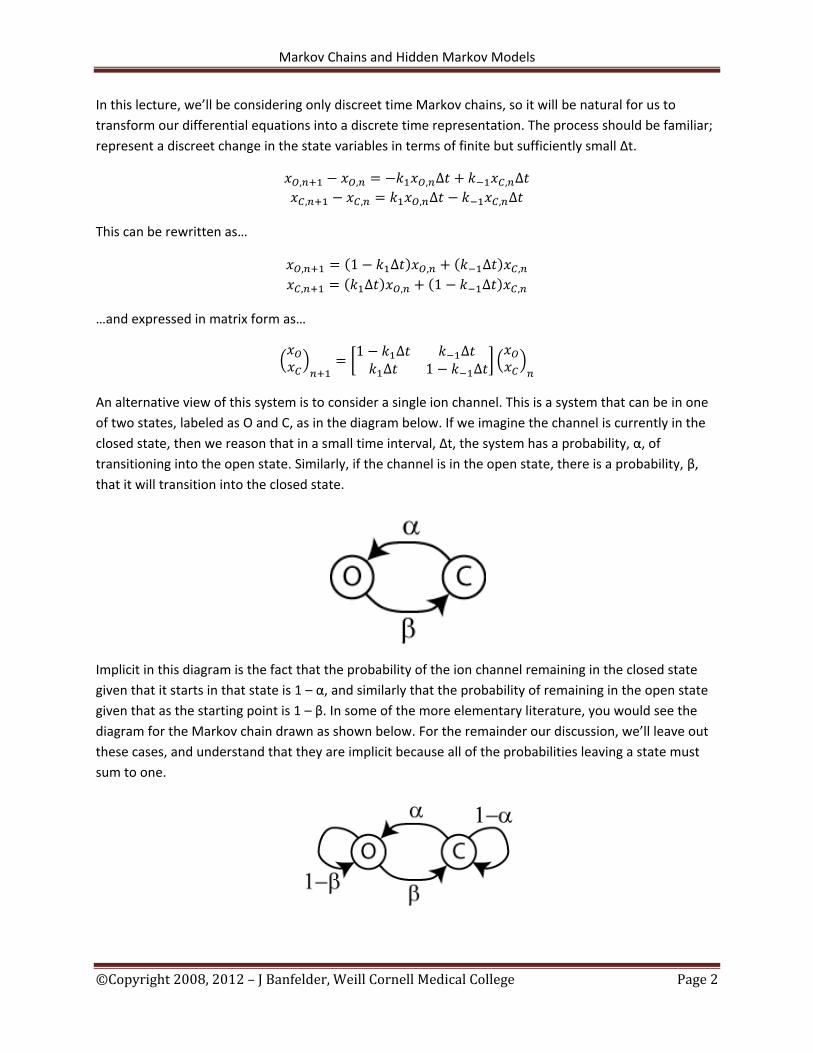
An alternative view of this system is to consider a single ion channel. This is a system that can be in one

of two states, labeled as O and C, as in the diagram below. If we imagine the channel is currently in the

closed state, then we reason that in a small time interval, Δt, the system has a probability, α, of

transitioning into the open state. Similarly, if the channel is in the open state, there is a probability, β,

that it will transition into the closed state.

Implicit in this diagram is the fact that the probability of the ion channel remaining in the closed state

given that it starts in that state is 1 – α, and similarly that the probability of remaining in the open state

given that as the starting point is 1 – β. In some of the more elementary literature, you would see the

diagram for the Markov chain drawn as shown below. For the remainder our discussion, we’ll leave out

these cases, and understand that they are implicit because all of the probabilities leaving a state must

sum to one.



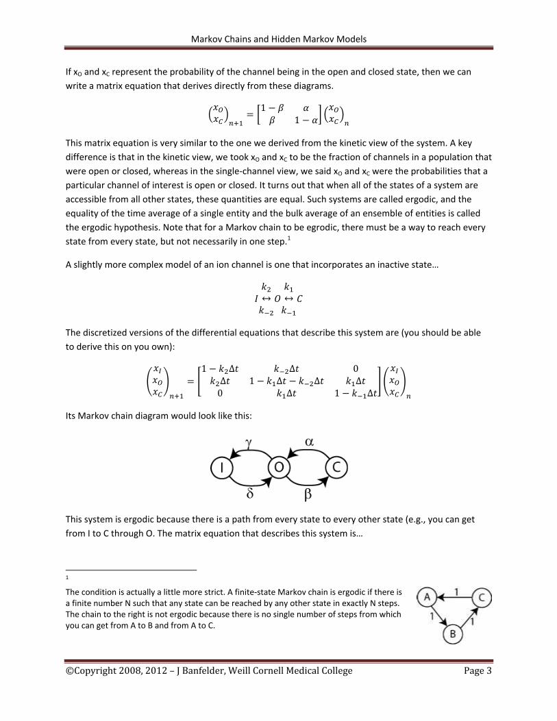
If xO and xC represent the probability of the channel being in the open and closed state, then we can

write a matrix equation that derives directly from these diagrams.

( )

[

] ( )

This matrix equation is very similar to the one we derived from the kinetic view of the system. A key

difference is that in the kinetic view, we took xO and xC to be the fraction of channels in a population that

were open or closed, whereas in the single-channel view, we said xO and xC were the probabilities that a

particular channel of interest is open or closed. It turns out that when all of the states of a system are

accessible from all other states, these quantities are equal. Such systems are called ergodic, and the

equality of the time average of a single entity and the bulk average of an ensemble of entities is called

the ergodic hypothesis. Note that for a Markov chain to be egrodic, there must be a way to reach every

state from every state, but not necessarily in one step.1

A slightly more complex model of an ion channel is one that incorporates an inactive state…

The discretized versions of the differential equations that describe this system are (you should be able

to derive this on you own):

(

)

[

] (

)

Its Markov chain diagram would look like this:

This system is ergodic because there is a path from every state to every other state (e.g., you can get

from I to C through O. The matrix equation that describes this system is…

1 The condition is actually a little more strict. A finite-state Markov chain is ergodic if there is a finite number N such that any state can be reached by any other state in exactly N steps. The chain to the right is not ergodic because there is no single number of steps from which you can get from A to B and from A to C.



(

)

[

](

)

For both the two and three state systems, you can see there is a direct correspondence between the

kinetic rate constants and the transition probabilities. If you know the transition probabilities for a

specific Δt, then you know the rate constants, and vice-versa.

A significant motivation for using Markov chains is that it gives us tools for systematically determining

the transition probabilities for complex systems. For the two canonical ion channel systems above, it is

pretty easy to design voltage clamp experiments that allow for the determination of the rates. However,

for more realistic and complex models, this becomes increasingly difficult. For example, Clancy and Rudy

(1999) proposed a model that included three closed states and both a fast and a slow inactive state:

The key characteristic of Markov processes is that the probability of transiting to the next state is

dependent ONLY on the current state. In other words, the system has no memory. This is known as the

Markov property.

We should also point out that for many ion channels of physiological importance, the transition

probabilities are voltage dependent. In the other words, α, β, γ, and δ are all functions of voltage. We

will only consider process were the elements of the transition matrix are constant over time (as in an

experiment with the voltage clamped).

Absorbing Markov chains Not all Markov processes are ergodic. An important class of non-ergodic Markov chains is the absorbing

Markov chains. These are processes where there is at least one state that can’t be transitioned out of;

you can think if this state as a trap. Some processes have more than one such absorbing state.

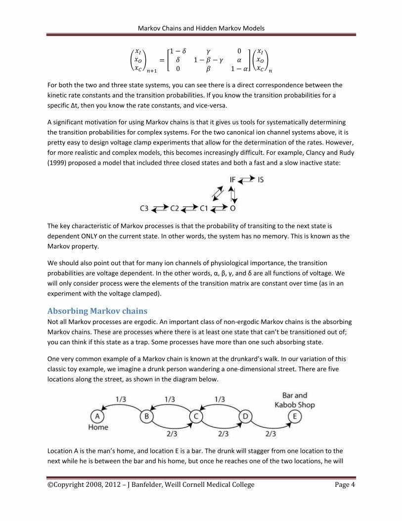
One very common example of a Markov chain is known at the drunkard’s walk. In our variation of this

classic toy example, we imagine a drunk person wandering a one-dimensional street. There are five

locations along the street, as shown in the diagram below.

Location A is the man’s home, and location E is a bar. The drunk will stagger from one location to the

next while he is between the bar and his home, but once he reaches one of the two locations, he will



stay there permanently (or at least for the night). The drunkard’s walk is usually presented where the

probability of moving to the left of right is equal, but in our scenario, we’ll say that the probability of

moving to the right is 2/3 because the pleasant odors emanating from the kabob shop next to the bar

serve as an attractant.

We can write a matrix equation to model our drunkard’s wanderings:

[ ] [ ]

[

]

Note that in this case we’ve written the state variables of our system (the probabilities that our

drunkard is at any of the five positions along the street) as a row vector. This follows the convention

used in most of the literature on Markov models, so we’ve adopted it here, and we’ll use it for the rest

of this lecture. As a consequence, our equations to describe the time evolution multiply the transition

matrix on the left. Also, the matrix in this representation is the transpose of the matrix we’d have

written if we were using column vectors. When written like this, all of the rows of the transition matrix

must sum to one.

We can use results from the theory of Markov chains to quickly answer some interesting questions

about a particular absorbing chain. We’ll look at three such questions: how to compute the number of

times each particular state is likely to be visited, how long a system is likely to last before being

absorbed, and what the probability of being absorbed into each of the absorbing states is. In general,

the answer to each of these questions is dependent on where you start on the chain.

Before we answer any of these questions, we’ll need to re-arrange our transition matrix into a canonical

form. All we need to do is reorder the states so that the transient ones are first, and the absorbing ones

come last. For our example problem, we have…

[ ] [ ]

[

]



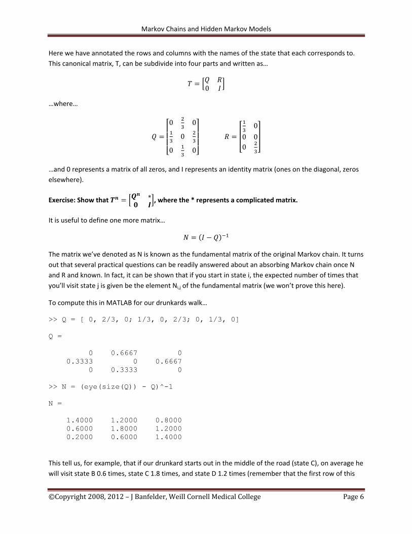
Here we have annotated the rows and columns with the names of the state that each corresponds to.

This canonical matrix, T, can be subdivide into four parts and written as…

[

]

…where…

[

]

[

]

…and 0 represents a matrix of all zeros, and I represents an identity matrix (ones on the diagonal, zeros

elsewhere).

Exercise: Show that [

], where the * represents a complicated matrix.

It is useful to define one more matrix…

( )

The matrix we’ve denoted as N is known as the fundamental matrix of the original Markov chain. It turns

out that several practical questions can be readily answered about an absorbing Markov chain once N

and R and known. In fact, it can be shown that if you start in state i, the expected number of times that

you’ll visit state j is given be the element Ni,j of the fundamental matrix (we won’t prove this here).

To compute this in MATLAB for our drunkards walk…

>> Q = [ 0, 2/3, 0; 1/3, 0, 2/3; 0, 1/3, 0]

Q =

0 0.6667 0

0.3333 0 0.6667

0 0.3333 0

>> N = (eye(size(Q)) - Q)^-1

N =

1.4000 1.2000 0.8000

0.6000 1.8000 1.2000

0.2000 0.6000 1.4000

This tell us, for example, that if our drunkard starts out in the middle of the road (state C), on average he

will visit state B 0.6 times, state C 1.8 times, and state D 1.2 times (remember that the first row of this



matrix corresponds to state B, the second to state C, and the last to state D). Note that the quantity for

C includes the starting visit.

We can also compute the average absorption time for each starting state. This is trivial if we know N. For

example, consider starting in state C. We just saw that the quantities in the second row of N give the

average number of times each transient state will be visited, so the sum of all of these entries must be

the average number of visits to all transient states. But the number of transient states one visits before

being absorbed is the absorption time.

A column vector, t, that represents the sum of row entries in the fundamental matrix can be written as..

…where c is a column vector of ones. Continuing the example above in MATLAB…

>> t = N * ones(size(N,1),1) t = 3.4000 3.6000 2.2000

This shows that if our drunkard starts at state B, on average the drunkard will stagger around for 3.4

steps before finishing up the evening at home or at the bar.

We can also compute the absorption probability matrix, B, simply by multiplying N on the right by R. The

elements of B give the probability of ultimately being absorbed into each of the absorbing states for

each starting state. In our example…

[

]

[

]

[

]

These results tell us that if we start at state B, for example, there is a 46.7% chance that we’ll eventually

absorb into state A, and a 53.3% change that we’ll absorb into state E.

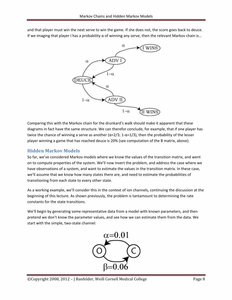
The drunkard’s walk is clearly a hypothetical problem, but examples just like it appear in many other

contexts. For example, consider a tennis game at deuce (e.g., tied at 40-40). The rules of tennis require

that a game be won by two serves. If player I wins the next serve, the score is said to be “Advantage I”,



and that player must win the next serve to win the game. If she does not, the score goes back to deuce.

If we imaging that player I has a probability α of winning any serve, then the relevant Markov chain is…

Comparing this with the Markov chain for the drunkard’s walk should make it apparent that these

diagrams in fact have the same structure. We can therefor conclude, for example, that if one player has

twice the chance of winning a serve as another (α=2/3; 1-α=1/3), then the probability of the lesser

player winning a game that has reached deuce is 20% (see computation of the B matrix, above).

Hidden Markov Models So far, we’ve considered Markov models where we know the values of the transition matrix, and went

on to compute properties of the system. We’ll now invert the problem, and address the case where we

have observations of a system, and want to estimate the values in the transition matrix. In these case,

we’ll assume that we know how many states there are, and need to estimate the probabilities of

transitioning from each state to every other state.

As a working example, we’ll consider this in the context of ion channels, continuing the discussion at the

beginning of this lecture. As shown previously, the problem is tantamount to determining the rate

constants for the state transitions.

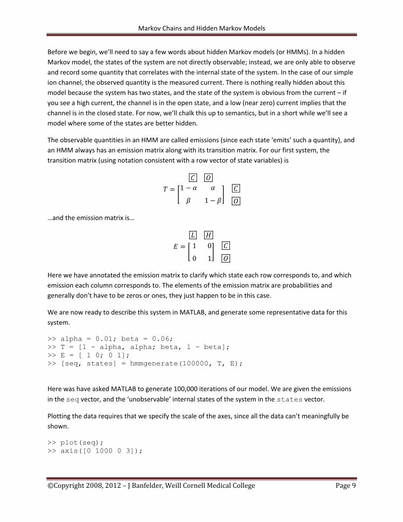
We’ll begin by generating some representative data from a model with known parameters, and then

pretend we don’t know the parameter values, and see how we can estimate them from the data. We

start with the simple, two-state channel:



Before we begin, we’ll need to say a few words about hidden Markov models (or HMMs). In a hidden

Markov model, the states of the system are not directly observable; instead, we are only able to observe

and record some quantity that correlates with the internal state of the system. In the case of our simple

ion channel, the observed quantity is the measured current. There is nothing really hidden about this

model because the system has two states, and the state of the system is obvious from the current – if

you see a high current, the channel is in the open state, and a low (near zero) current implies that the

channel is in the closed state. For now, we’ll chalk this up to semantics, but in a short while we’ll see a

model where some of the states are better hidden.

The observable quantities in an HMM are called emissions (since each state ‘emits’ such a quantity), and

an HMM always has an emission matrix along with its transition matrix. For our first system, the

transition matrix (using notation consistent with a row vector of state variables) is

[

]

…and the emission matrix is…

[

]

Here we have annotated the emission matrix to clarify which state each row corresponds to, and which

emission each column corresponds to. The elements of the emission matrix are probabilities and

generally don’t have to be zeros or ones, they just happen to be in this case.

We are now ready to describe this system in MATLAB, and generate some representative data for this

system.

>> alpha = 0.01; beta = 0.06;

>> T = [1 - alpha, alpha; beta, 1 - beta];

>> E = [ 1 0; 0 1];

>> [seq, states] = hmmgenerate(100000, T, E);

Here was have asked MATLAB to generate 100,000 iterations of our model. We are given the emissions

in the seq vector, and the ‘unobservable’ internal states of the system in the states vector.

Plotting the data requires that we specify the scale of the axes, since all the data can’t meaningfully be

shown.

>> plot(seq);

>> axis([0 1000 0 3]);



You can pan to the right to see more of the trace. As a side note here, you should be aware that when

make a plot that has more datapoints than your screen has pixels, your plotting program may entirely

miss artifacts in your data (this depends on how your software samples the data for plotting).

Note that in the plot produced, there are some long periods of low current and some short periods of

low current, and similarly for the periods of high current. We says that the dwell times for each state

follow some distribution. It should be clear from the plot that the closed states tend to last longer than

the open states. This implies that β > α, which is in fact the case.

Note that MATLAB numbers the states and emissions from 1, so an emission value of 1 corresponds to

the low current emission, and an emission value of 2 represents a high current emission.

Formally, an HMM consists of a transition matrix, an emissions matrix, and a starting state. When using

MATLAB’s HMM functions, it is assumed that the system always starts in state 1. You can always

rearrange the states to accommodate (or see the MATLAB help for other tricks).

Now that we have generated a good amount of trace data (representative of a single channel

recording), out goal is to recover the α and β parameters from the trace data alone. For this simple

model, there are several approaches. One way to go about this is to analyze the distributions of the

dwell times in the open and closed states. To this end, we can write a function which reports the dwell

times for a particular emission. The source code is kept in a file named dwell_times.m:

function [ times ] = dwell_times(seq,s) %DWELL_TIMES Given a sequence of states (seq), % compute the dwell times state s in the sequence.

imax = length(seq); times = [];

previous_state = seq(1); counter = 0;

for idx = 2:imax if(previous_state == seq(idx)) counter = counter + 1; else if (previous_state == s) times = [times ; counter]; end counter = 1; previous_state = seq(idx); end end

end

We can now compute the dwell times for the low current state.



>> dt_closed = dwell_times(seq, 1);

>> mean(dt_closed)

ans =

96.6472

This is telling us that the average dwell time in the low current state is 96.6. The reciprocal of this is our

estimate of the time constant, or transition probability, to leave the closed to the open state. We

therefore estimate that α = 1/96.6472 = 0.0103. Similarly, in this example, we estimate the β = 0.0642

from the distribution of dwell times in the open state.

In this example, we were able to make these estimates because we can trivially infer the state of the

channel from its emission measurement. We’ll now consider a slightly more complicated channel model

where (some of) the states are hidden.

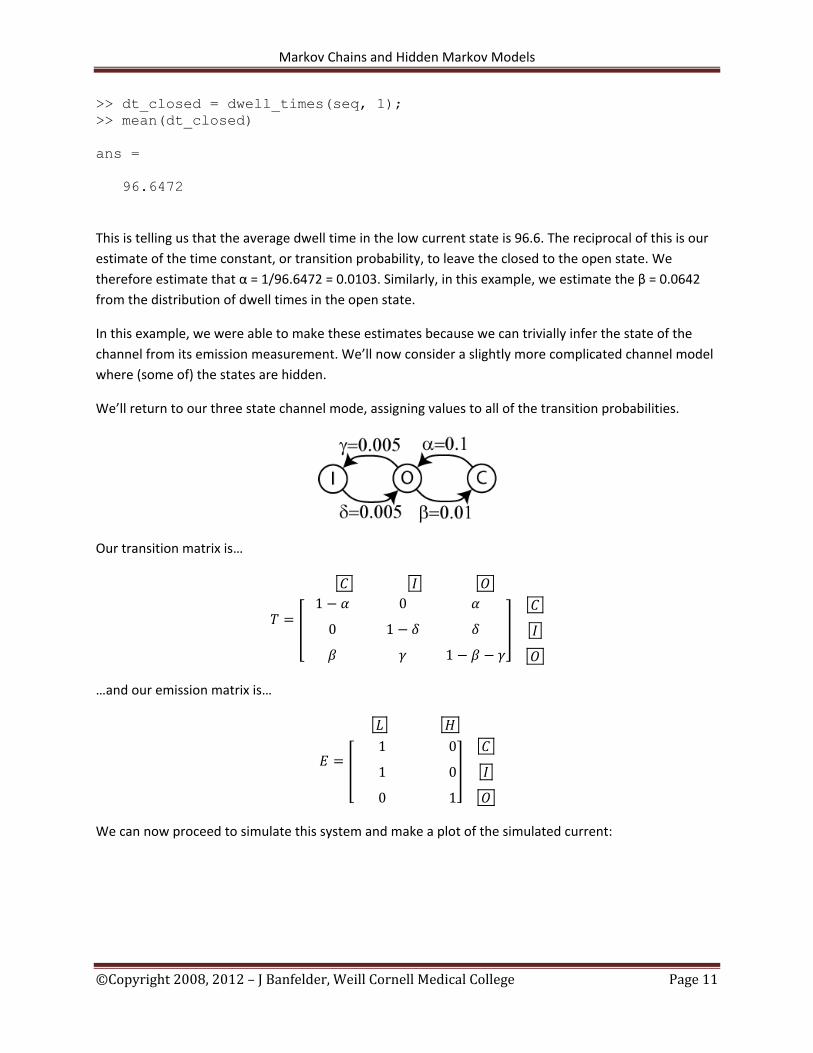
We’ll return to our three state channel mode, assigning values to all of the transition probabilities.

Our transition matrix is…

[

]

…and our emission matrix is…

[

]

We can now proceed to simulate this system and make a plot of the simulated current:



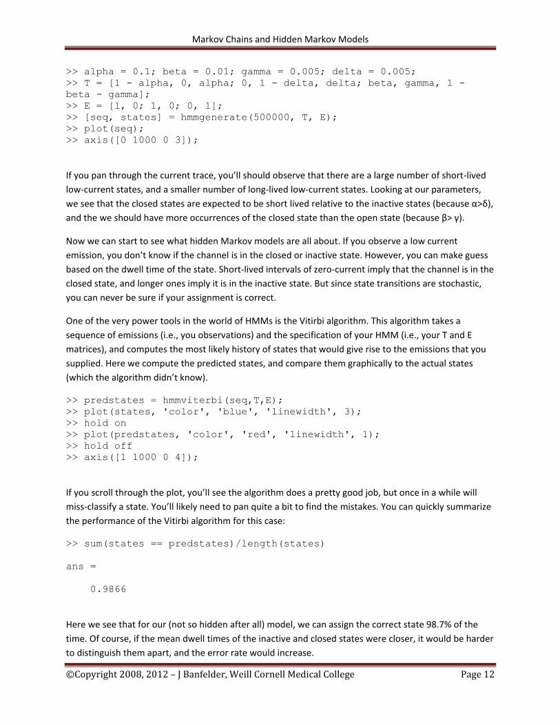
>> alpha = 0.1; beta = 0.01; gamma = 0.005; delta = 0.005;

>> T = [1 - alpha, 0, alpha; 0, 1 - delta, delta; beta, gamma, 1 -

beta - gamma];

>> E = [1, 0; 1, 0; 0, 1];

>> [seq, states] = hmmgenerate(500000, T, E);

>> plot(seq);

>> axis([0 1000 0 3]);

If you pan through the current trace, you’ll should observe that there are a large number of short-lived

low-current states, and a smaller number of long-lived low-current states. Looking at our parameters,

we see that the closed states are expected to be short lived relative to the inactive states (because α>δ),

and the we should have more occurrences of the closed state than the open state (because β> γ).

Now we can start to see what hidden Markov models are all about. If you observe a low current

emission, you don’t know if the channel is in the closed or inactive state. However, you can make guess

based on the dwell time of the state. Short-lived intervals of zero-current imply that the channel is in the

closed state, and longer ones imply it is in the inactive state. But since state transitions are stochastic,

you can never be sure if your assignment is correct.

One of the very power tools in the world of HMMs is the Vitirbi algorithm. This algorithm takes a

sequence of emissions (i.e., you observations) and the specification of your HMM (i.e., your T and E

matrices), and computes the most likely history of states that would give rise to the emissions that you

supplied. Here we compute the predicted states, and compare them graphically to the actual states

(which the algorithm didn’t know).

>> predstates = hmmviterbi(seq,T,E);

>> plot(states, 'color', 'blue', 'linewidth', 3);

>> hold on

>> plot(predstates, 'color', 'red', 'linewidth', 1);

>> hold off

>> axis([1 1000 0 4]);

If you scroll through the plot, you’ll see the algorithm does a pretty good job, but once in a while will

miss-classify a state. You’ll likely need to pan quite a bit to find the mistakes. You can quickly summarize

the performance of the Vitirbi algorithm for this case:

>> sum(states == predstates)/length(states)

ans =

0.9866

Here we see that for our (not so hidden after all) model, we can assign the correct state 98.7% of the

time. Of course, if the mean dwell times of the inactive and closed states were closer, it would be harder

to distinguish them apart, and the error rate would increase.



Our last application of HMMs will be to demonstrate a training algorithm. The job of the training

algorithm is to determine the values in the state transition matrix and the emission matrix given a trace

of sequences. This is an iterative procedure, so it will require an initial guess for these two matrices. In

our example, the emission matrix is simple and the guess is obvious. However, guessing the transition

probabilities from only the simulated data is a bit trickier.

We’ll begin by computing the dwell-times as before.

>> dt_low = dwell_times(seq, 1);

>> dt_high = dwell_times(seq,2);

Now the structure of our model tells us that we should expect two classes of non-conducting states with

different dwell-time distributions. We might suspect that a histogram of the dwell times would have two

peaks, but trying out a few plots doesn’t yield anything obvious. However, a histogram of the logarithm

of the dwell time is informative.

>> hist(log(dt_low), 0:0.1:10)

You should see a peak very roughly around 2.5 and a peak around 5. This implies that there are two

(somewhat hidden) peaks at e2.5 = 12.2 and e5 = 148. So our very rough guesses of the transition

probabilities are α= 1/12.2 = 0.08 and δ = 1/148 = 0.007. We also need to guess β and γ; since the

training algorithm will do the heavy lifting, we’ll assume that β = γ. Now the average dwell time for the

conducting state is…

>> mean(dt_high)

ans =

67.3133

…so we have that β + γ (the two ways we can leave the open state) = 1/67.3 = 0.0149 so we guess β = γ

= 0.0149 / 2 = 0.0074. We are now ready to run the training algorithm:

>> alphag = 0.08; betag = 0.0074; gammag = 0.0074; deltag = 0.007;

>> Tg = [ 1 - alphag, 0, alphag; 0, 1 - deltag, deltag; betag, gammag,

1 - betag - gammag];

>> Eg = E;

>> [T_estimate, E_estimate] = hmmtrain(seq, Tg, Eg);

The training algorithm may take a little while to finish, but when it does, we can compare the estimated

transition matrix with the one from which the sample data was derived:



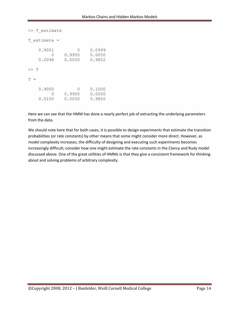
>> T_estimate

T_estimate =

0.9001 0 0.0999

0 0.9950 0.0050

0.0098 0.0050 0.9852

>> T

T =

0.9000 0 0.1000

0 0.9950 0.0050

0.0100 0.0050 0.9850

Here we can see that the HMM has done a nearly perfect job of extracting the underlying parameters

from the data.

We should note here that for both cases, it is possible to design experiments that estimate the transition

probabilities (or rate constants) by other means that some might consider more direct. However, as

model complexity increases, the difficulty of designing and executing such experiments becomes

increasingly difficult; consider how one might estimate the rate constants in the Clancy and Rudy model

discussed above. One of the great utilities of HMMs is that they give a consistent framework for thinking

about and solving problems of arbitrary complexity.

markov chains and hidden markov models - cornell...

Documents