markov chains, markov processes, queuing theory and ...anthonybusson.fr/fileteaching/markov.pdf ·...
TRANSCRIPT
Markov chains, Markov Processes, Queuing Theory
and Application to Communication Networks
Anthony Busson,University Lyon 1 - Lyon - [email protected]
November 17, 2016
Contents
1 Markov Chains 21.1 Definitions and properties . . . . . . . . . . . . . . . . . . . . 21.2 Distribution of a Markov chain. . . . . . . . . . . . . . . . . . 41.3 A first queue . . . . . . . . . . . . . . . . . . . . . . . . . . . 11
2 Markov Processes 132.1 Properties of the exponential distribution. . . . . . . . . . . . 132.2 Distribution of a Markov process. . . . . . . . . . . . . . . . . 152.3 Equilibrium distribution of a Markov process. . . . . . . . . . 20
3 Jump chain 233.1 A natural jump chain . . . . . . . . . . . . . . . . . . . . . . 233.2 Other jump chains . . . . . . . . . . . . . . . . . . . . . . . . 25
4 Queuing Theory 264.1 Kendall Notation . . . . . . . . . . . . . . . . . . . . . . . . . 264.2 M/M/1 . . . . . . . . . . . . . . . . . . . . . . . . . . . . . . 274.3 M/M/K . . . . . . . . . . . . . . . . . . . . . . . . . . . . . . 294.4 M/M/+∞ . . . . . . . . . . . . . . . . . . . . . . . . . . . . . 304.5 M/M/K/K+C . . . . . . . . . . . . . . . . . . . . . . . . . . 304.6 Some interesting results . . . . . . . . . . . . . . . . . . . . . 314.7 M/GI/1 and GI/M/1 . . . . . . . . . . . . . . . . . . . . . . . 34
5 Miscellaneous 35
1

1 Markov Chains
1.1 Definitions and properties
Exercise 1. We consider a flea moving along the points of an axis. Theposition of the flea on the axis is represented by a positive integer. The fleais initially at the origin 0. If the flea is at position i (with i 6= 0) at somestage, it moves with probability p (0 < p < 1) on its right (from i to i+ 1),and with probability 1 − p on its left. The flea necessarily moves at eachstage (it cannot stay at the same location).
1. What is the probability that the flea moves to position 1 if it is currentlyat 0?
2. If after n steps, the flea is at position k, what is the probability of itbeing at position i at the n+ 1th step?
3. What is the probability that the flea is at position i at the n+ 1th stepwithout having knowledge of the past?
Answers
1. The flea has only one possibility. It can only move to position 1.Therefore, the probability to move to 1 is 1 and hence the probabilityto move to any other position is 0.
2. The probability to move from position k to k+1 is p and the probabilityto move from k to k − 1 is 1 − p (that’s given by the subject of theexercise). For any other positions, the probability is nill.
3. If we know only the initial location of the flea (it is 0 for this exercise),we have to look at all the possible trajectories from 0 to i in n+1 steps.The Markov chain offers a Mathematical (and practical) framework todo that.
Definition 1. Markov Chain. Let (Xn)n∈IN be a sequence of randomvariables taking values in a countable space E (in our case we will take INor a subset of IN). (Xn)n∈IN is a Markov chain if and only if
P(Xn = in|Xn−1 = in−1, Xn−2 = in−2, .., X0 = i0) = P(Xn = in|Xn−1 = in−1)
Thus for a Markov chain, the state of the chain at a given time containsall the information about the past evolution which is of use in predicting itsfuture behavior. We can also say that given the present state, the past andthe future are independent.
Definition 2. Homogeneity. A Markov chain is homogeneous if andonly if P(Xn = j|Xn−1 = i) does not depend on n.
2

Definition 3. Irreducibility. A Markov chain is irreducible if and onlyif every state can be reached from every other state.
Definition 4. Transition probabilities. For a homogeneous Markov chain,
pj,i = P(Xn = i|Xn−1 = j)
is called the transition probability from state j to state i.
Definition 5. Period. A state i is periodic if there exists an integer δ > 1such that P(Xn+k = i|Xn = i) = 0 unless k is divisible by δ ; otherwisethe state is aperiodic. If all the states of a Markov chain are periodic(respectively aperiodic), then the chain is said to be periodic (respectevilyaperiodic).
Exercise 2. We consider a player playing ”roulette” in a casino. Initiallythe player has N dollars. For each spin, he bets 1 dollar on red. Let Xn bethe process describing the amount of money that the player has after n bets.
1. Is Xn a Markov chain?
2. In case of a Markov chain, what are the transition probabilities? Arethe states periodic or aperiodic? Is it irreducible?
3. What is the distribution of Xn with regard to Xn−1, and Xn with regardto Xn−2 ?
Answers
1. Xn is a Markov chain. Given the value of Xn−1, we can express thedistribution of Xn whatever the value of Xk for k < n− 1.
2. The transition probabilities are
pi,i+1 =Number of red compartments
Total number of compartments
pi,i−1 =Number of black and green compartments
Total number of compartments
The number of compartments is 37 in France and 38 in USA. Bothhave 18 red and black compartments but in USA there are two zeros(0 and 00). So, in France, we get pi,i+1 = 18
37 and pi,i−1 = 1937 . For the
USA, we get pi,i+1 = 1838 and pi,i−1 = 20
38 .The period can be seen as the minimum number of steps required toreturn to the same state. For the above case, we can come back atstate j only after an even number of steps (except for the state 0).The period is then 2 for all the states (except state 0). The chain isnot irreducible (irreducible means that for all (i, j), there is at least
3
one trajectory from i to j with positive probability). Indeed, once Xn
has reached 0, the player hasn’t got anymore money. The state 0 istherefore an absorbant state since the chain stays in this state for therest of the time.
3. The distribution of Xn with regard to Xn−1 is given by the transitionprobabilities. The distribution of Xn w.r.t. Xn−2 is obtained by condi-tionning the possible values of Xn−1 (if we look at the probability thatXn = i, the only possible values of Xn−1 for which the probability isnot 0 is Xn−1 = i− 1 and Xn−1 = i+ 1):
P (Xn = i|Xn−2 = j)
= P (Xn = i,Xn−1 = i− 1|Xn−2 = j) + P (Xn = i,Xn−1 = i+ 1|Xn−2 = j)
= P (Xn = i|Xn−1 = i− 1, Xn−2 = j)P (Xn−1 = i− 1|Xn−2 = j)
+P (Xn = i|Xn−1 = i+ 1, Xn−2 = j)P (Xn−1 = i+ 1|Xn−2 = j) using Baye’s formula
= P (Xn = i|Xn−1 = i− 1)P (Xn−1 = i− 1|Xn−2 = j)
+P (Xn = i|Xn−1 = i+ 1)P (Xn−1 = i+ 1|Xn−2 = j) using Markov property
= pi−1,ipj,i−1 + pi+1,ipj,i+1
The only values of j for which the equality above will not be nill arej = i − 2, i, i + 2. Let note pi,i−1 = p and pi,i+1 = 1 − p (it does notdepend on i), we get
P (Xn = i|Xn−2 = i− 2) = p2
P (Xn = i|Xn−2 = i) = 2p(1− p)P (Xn = i|Xn−2 = i+ 2) = (1− p)2
Exercise 3. Give an example of a periodic Markov chain.Answer We have seen that the Markov chain of exercise 2 has all its
states periodic with period 2 except 0. To have all the states of the sameperiod, we just have to change the transition probability of state 0 in such away that its period is 2. Let p0,1 = 1 (rather than p0,0 = 1) and we obtaina Markov chain with period 2. Note that if the chain is irreducible, all thestates have the same period. When we changed the transition probability ofstate 0, the chain became irreducible.
1.2 Distribution of a Markov chain.
Definition 6. We define the distribution vector Vn of Xn as
Vn = (P(Xn = 0),P(Xn = 1),P(Xn = 2), ..)
Exercise 4. Let Vn be the distribution vector of a Markov chain Xn.
1. Express vector Vn as function of Vn−1 and the transition matrix P.
4
2. Express Vn as function of V0 and P .
Answers
1. We consider a Markov chain Xn which takes its values from {0, 1, 2, .., N}(the method would be the same for any countable space) with transitionmatrix P . We are going to express Vn(i) with regard to Vn−1 and P .Conditionning by the values of Xn−1, we obtain:
Vn(i) = P (Xn = i)
=N∑j=0
P (Xn = i,Xn−1 = j)
=
N∑j=0
P (Xn = i|Xn−1 = j)P (Xn−1 = j) Baye’s formulae
=N∑j=0
pj,iVn−1(j)
The above equation can be easily express in matrix form:
Vn = Vn−1P
2. A simple recursive process gives the result:
Vn = Vn−1P
= Vn−2P2
= V0Pn
So a simple way to compute the probability that {Xn = i} is to compute∑j∈E V0(j)p
(n)j,i . More generally, we get (if we stop the recurrence after
k steps):
Vn(i) =∑j∈E
Vn−k(j)p(n−k)j,i (The Chapman-Kolmogorov equation)
It is important to note that p(k)j,i is the element (i, j) of the matrix P k
and not the element pj,i to the power k of the matrix P .
Exercise 5. We consider a Markov chain that take its value from the set{0, 1}. The transition matrix is(
p 1− p1− q q
)
5
What is the limit of Vn when n tends to infinity? Compute Vn with p = q =12 .
Answers From exercise 4, we know that Vn = V0Pn. One way to compute
Vn is to ”diagonalize” the matrix P . In other words, we break up P asP = QDQ−1 where D is a diagonal matrix and Q is invertible. Hence, wecan write
Vn = V0QDnQ−1
The eigenvalues of P are the roots of the equation det(P−λI) = 0, wheredet() is the determinant, I is the identity matrix with same dimensions asthat of P and λ is a scalar. We obtain for our example:
det(P − λI) = λ2 − λ(p+ q)− (1− p− q)
The two roots of this equation are λ1 = 1 and λ2 = −(1−q−p). The matrixD is therefore
D =
(1 00 −(1− q − p)
)The eigenvectors can be found by solving the equation (P − λ1I)X = 0
(resp. λ2) with x = (x1, x2). For λ1, we get
(p− 1)x1 + (1− p)x2 = 0
(1− q)x1 + (q − 1)x2 = 0
The two equations are redundant, it suffices to find a vector (x1, x2)which verifies one of the two equations. We choose x1 = 1 and x2 = 1.The first eigenvector is therefore E1 = (1, 1)T . Similar computations lead toE2 = (1,− 1−q
1−p)T . The matrix Q and Q−1 are then
Q =
(1 1
1 − 1−q1−p
)and
Q−1 =
(1−q
1−p+1−q1−p
1−p+1−q1−p
1−p+1−q − 1−p1−p+1−q
)From these expressions, it is very easy to compute Vn for all n. If p =
q = 12 , we get
D =
(1 00 0
)
Q−1 =
(12
12
12 −1
2
)
6
and
Q =
(1 11 −1
)Since for this particular case, Dn = D, we obtain
Vn = V0
(12
12
12
12
)and Vn = (12 ,
12) whatever the values of V0. We have seen through this
simple example, that the diagonalization of transition matrix is not an easytask. When the space E has a much greater number of elements (note thatit can also be infinite), the diagonalization is even impossible. Moreover, inpractical cases, we are not interested in the distribution of Vn for small nbut rather for large n or for the asymptotic behavior of the Markov chain.We will see that under certain assumptions, the distribution of Vn reachesan equilibrium state which is clearly easier to compute.
Definition 7. If Xn has the same distribution vector as Xk for all (k, n) ∈IN2, then the Markov chain is stationary.
Exercise 6. Let (Xn)n∈IN be a stationary Markov chain. Find an equationthat the distribution vector should verify.
Theorem 1. Let (Xn)n∈IN be a Markov chain. We assume that Xn isirreducible, aperiodic and homogeneous. The Markov chain may possess anequilibrium distribution also called stationary distribution , that is,a distribution vector π (with π = (π0, π1, ...)) that satisfies
πP = π (1)
and ∑k∈E
πk = 1 (2)
If we can find a vector π satisfying equations (1) and (2), then thisdistribution is unique and
limn→+∞
P (Xn = i|X0 = j) = πi
so that π is the limiting distribution of the Markov chain.
Theorem 2. Ergodicity. Let (Xn)n∈IN be a Markov chain. We assume thatXn is irreducible, aperiodic and homogeneous. If a Markov chain possesses
7

an equilibrium distribution, then the proportion of time the Markov chainspends in state i during the period [0, n] converges to πi as n→ +∞:
limn→+∞
1
n
n∑k=0
1lXk=i = πi
In this case, we say that the Markov chain is ergodic.
Exercise 7. In this exercise, we give two examples of computation andinterpretation of the distribution obtained with equations 1 and 2 when theassumptions of theorem 1 does not hold.
1. Resume exercise 2 on roulette. Does the Markov chain possess anequilibrium distribution? Compute it.
2. Resume exercise 1 on the flea. Does the Markov chain possess anequilibrium distribution? Compute it.
Remark 1. Equilibrium distribution and periodicity. If the Markovchain is periodic, then there is no limit to the distribution vector. The solu-tion of equations (1) and (2) when it exists, is interpreted as the proportionof time that the chain spends in the different states.
Remark 2. Transient chain. If there is no solution to equations (1)and (2) for an aperiodic, homogeneous, irreducible Markov chain (Xn)n∈INthen there is no equilibrium distribution and
limn→+∞
P (Xn = i) = 0
Remark 3. The state of a Markov chain may be classified as transient orrecurrent.
1. A state i is said to be transient if, given that we start in state i,there is a non-zero probability that we will never return back to i.Formally, let the random variable Ti be the next return time to state i(Ti = min{n : Xn = i|X0 = i}), then state i is transient if and only ifthere exists a finite Ti such that
P (Ti < +∞) < 1
2. A state i will be recurrent if it is not transient (P (Ti < +∞) = 1).
In case of an irreducible Markov chain, all the states are either transientor recurrent. If the Markov chain possesses an equilibrium distribution, thenthe Markov chain is recurrent (all the states are recurrent) and πi = 1
E[Ti] .
8

Exercise 8. Resume exercise 1 on the flea. We assume now, that there isa probability p that the flea goes to the left, and a probability q that the fleastays at the current state (with p+ q < 1).
1. Express the transition matrix.
2. Is the Markov chain still periodic?
3. What is the condition of existence of a solution to equations (1) and (2)?Compute it.
AnswersThe transition matrix is:
P =
0 1 0 0 0 ...
1− q − p q p 0 0 ...0 1− q − p q p 0 ...0 0 1− q − p q p ...... ... ... ... ... ...
Equation πP = π leads to the following set of equations:
π1(1− q − p) = π0 (3)
π0 + qπ1 + (1− q − p)π2 = π1 (4)
pπ1 + qπ2 + (1− q − p)π3 = π2
...
pπk−1 + qπk + (1− q − p)πk+1 = πk (5)
From equations 3 and 4, we obtain
π1 =π0
1− q − pand π2 =
p
(1− q − p)2π0
We assume that πk can be written in the form πk = pk−1
(1−q−p)kπ0. To prove
this, we just have to verify that this form is a solution of equation 5 (it is ofcourse true). Now, the distribution has to verify equation 2:
+∞∑i=0
πi =
[1 +
+∞∑i=1
pi−1
(1− q − p)i
]π0
=
[1 +
1
(1− q − p)
+∞∑i=0
(p
(1− q − p)
)i]π0
The sum in the above equation is finite if and only if p < 1− q − p. In thiscase, we get (from
∑π1 = 1):
π0 =
[1 +
1
1− q − 2p
]−19

and
πk = π0pk−1
(1− q − p)k
If p > 1−q−p, the sum is infinite and π0 = 0, thus πi = 0 for all i. Theprocess is then transient. The flea tends to move away indefinitely from 0.
Exercise 9. Let (Xn)n∈IN be a Markov chain with E = 0, 1, 2, 3, 4 and withthe following transition matrix:
0 12
12 0 0
13 0 1
313 0
13
13 0 1
3 00 0 0 1
212
0 0 0 12
12
1. Solve equations (1) and (2) for this Markov chain.
2. What is the condition for the existence of a solution? Why?
Answers The equation πP = π leads to the following set of equations:
1
3π1 +
1
3π2 = π0
1
2π0 +
1
3π2 = π1
1
2π0 +
1
3π1 = π2 (6)
1
3π1 +
1
3π2 +
1
2π3 +
1
2π4 = π3 (7)
1
2π3 +
1
2π4 = π4 (8)
Equation 8 leads to π3 = π4. Substituting π3 = π4 in equation 7 leadsto π1 = π2 = 0 (since π1 and π2 cannot be negative). Putting π1 = π2 = 0in equation 6 leads to π0 = 0. Finally, we get π0 = π1 = π2 = 0 andπ3 = π4 = 1
2 . This is easily interpretable. If the chain goes in the state 3 or4, it stays indefinitly among these two states. Indeed, the probability to goto other states is nill. So, if the chain starts from a state among {0, 1, 2},it will stay in it for a finite number of steps, then (with probability 1) it willmove to the set {3, 4} and stay there for the rest of the time. The states{0, 1, 2} are transient and the other two states are recurrent. It is due to thefact that the chain is not irreducible. When we deal with a reducible chain,we generally consider only a subset of states (which are irreducible) and wecompute the stationnary distribution for this subset. In this exercise, theirreducible subset of states is {3, 4}.
10
1.3 A first queue
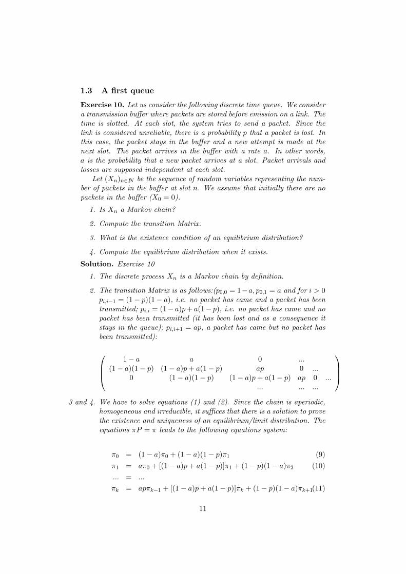
Exercise 10. Let us consider the following discrete time queue. We considera transmission buffer where packets are stored before emission on a link. Thetime is slotted. At each slot, the system tries to send a packet. Since thelink is considered unreliable, there is a probability p that a packet is lost. Inthis case, the packet stays in the buffer and a new attempt is made at thenext slot. The packet arrives in the buffer with a rate a. In other words,a is the probability that a new packet arrives at a slot. Packet arrivals andlosses are supposed independent at each slot.
Let (Xn)n∈IN be the sequence of random variables representing the num-ber of packets in the buffer at slot n. We assume that initially there are nopackets in the buffer (X0 = 0).
1. Is Xn a Markov chain?
2. Compute the transition Matrix.
3. What is the existence condition of an equilibrium distribution?
4. Compute the equilibrium distribution when it exists.
Solution. Exercise 10
1. The discrete process Xn is a Markov chain by definition.
2. The transition Matrix is as follows:(p0,0 = 1−a, p0,1 = a and for i > 0pi,i−1 = (1− p)(1− a), i.e. no packet has came and a packet has beentransmitted; pi,i = (1− a)p+ a(1− p), i.e. no packet has came and nopacket has been transmitted (it has been lost and as a consequence itstays in the queue); pi,i+1 = ap, a packet has came but no packet hasbeen transmitted):
1− a a 0 ...
(1− a)(1− p) (1− a)p+ a(1− p) ap 0 ...0 (1− a)(1− p) (1− a)p+ a(1− p) ap 0 ...
... ... ...
3 and 4. We have to solve equations (1) and (2). Since the chain is aperiodic,
homogeneous and irreducible, it suffices that there is a solution to provethe existence and uniqueness of an equilibrium/limit distribution. Theequations πP = π leads to the following equations system:
π0 = (1− a)π0 + (1− a)(1− p)π1 (9)
π1 = aπ0 + [(1− a)p+ a(1− p)]π1 + (1− p)(1− a)π2 (10)
... = ...
πk = apπk−1 + [(1− a)p+ a(1− p)]πk + (1− p)(1− a)πk+1(11)
11

Equation 9 (resp. 10) leads to the expression of π1 (resp. π2) as afunction of π0:
π1 =a
(1− a)(1− p)π0
π2 =a2p
(1− a)2(1− p)2π0
So, we assume that πk has the following form:
πk =akpk−1
(1− a)k(1− p)kπ0
We prove that by substituting this expression in the left-hand side ofequation (11):
(11) = apak−1pk−2
(1− p)k−1(1− a)k−1π0 + [(1− a)p+ a(1− p)] akpk−1
(1− p)k(1− a)kπ0
+(1− p)(1− a)ak+1pk
(1− p)k+1(1− a)k+1π0
= π0akpk−1
(1− p)k(1− a)k[(1− a)(1− p) + (1− a)p+ a(1− p) + ap]
= π0akpk−1
(1− p)k(1− a)k[(1− a)− (1− a)p+ (1− a)p+ a(1− p) + ap]
= π0akpk−1
(1− p)k(1− a)k[1]
The sum must be one.
+∞∑k=0
πk = π0
[1 +
+∞∑k=1
1
p
(ap
(1− a)(1− p)
)k]
= π0
[1 +
1
p
(ap
(1− a)(1− p)
) +∞∑k=0
(ap
(1− a)(1− p)
)k]
= π0
[1 +
1
p
(ap
(1− a)(1− p)
)1
1− ap(1−a)(1−p)
]The last equality is true only if the term to the power k is strictly lessthan 1. Otherwise the sum does not converge. The condition for theexistence of an equilibrium distribution is then ap < (1 − a)(1 − p)leading to 1−p > a. So, the probability of arrival MUST BE less thanthe probability of transmission success. It is obvious that otherwise,the buffer will fill infinitely. The last equation gives the expression forπ0 and the final expression of πk depends only on p and a.
12
2 Markov Processes
In this Section, we introduce the definition and main results for Markovprocesses. A Markov process is a random process (Xt)t∈φ indexed by acontinuous space (it is indexed by a discrete space for the Markov chains)and taking values in a countable space E. In our case, it will be indexedby IR+ (φ = IR+). In this course, we are only interested in non explosiveMarkov processes (also called regular processes), i.e. processes which arecapable of passing through an infinite number of states in a finite time. Inthe definition below, we give the property that a random process must verifyto be a Markov process.
Definition 8. The random process or stochastic process (Xt)t∈IR+ is aMarkov process if and only if, for all (t1, t2, ...tn) ∈ (IR+)n such thatt1 < t2 < t3 < ... < tn−1 < tn and for (i1, ..., in) ∈ En,
P(Xtn = in|Xtn−1 = in−1, Xtn−2 = in−2, ..., Xt1 = i1) =
P(Xtn = in|Xtn−1 = in−1
)A Markov process is time homogeneous if P (Xt+h = j|Xt = i) does
not depend on t. In the following, we will consider only homogeneous Markovprocess.
The interpretation of the definition is the same as in the discrete case(Markov chain) ; Conditionally to the present the past and the future areindependent. From the Definition 8 of a Markov process, we obtain inSections 2.2 and 2.3 the main results on the Markov processes. But, webegin by giving some properties of the exponential distribution which playan important part in Markov process.
2.1 Properties of the exponential distribution.
Definition 9. The probability density function (pdf) of an exponentialdistribution with parameter µ (µ ∈ IR+) is
f(x) = µe−µx1lx≥0
The cumulative distribution function ( denoted cdf, defined as F (u) =P(T ≤ u)) of an exponential distribution with parameter µ is
F (u) =(1− e−µu
)1lu≥0
Proposition 1. Memorylessness. An important property of the expo-nential distribution is that it is memoryless. This means that if a randomvariable T is exponentially distributed, its conditional probability obeys
13
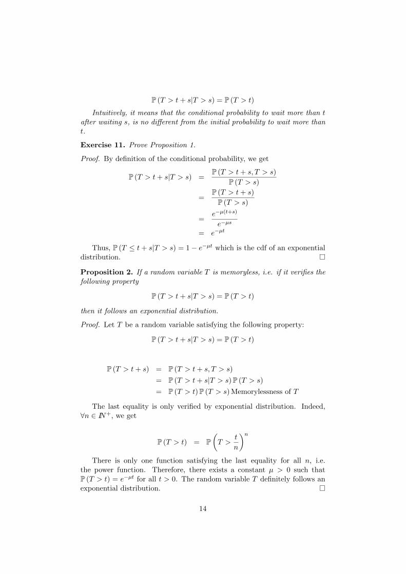
P (T > t+ s|T > s) = P (T > t)
Intuitively, it means that the conditional probability to wait more than tafter waiting s, is no different from the initial probability to wait more thant.
Exercise 11. Prove Proposition 1.
Proof. By definition of the conditional probability, we get
P (T > t+ s|T > s) =P (T > t+ s, T > s)
P (T > s)
=P (T > t+ s)
P (T > s)
=e−µ(t+s)
e−µs
= e−µt
Thus, P (T ≤ t+ s|T > s) = 1− e−µt which is the cdf of an exponentialdistribution.
Proposition 2. If a random variable T is memoryless, i.e. if it verifies thefollowing property
P (T > t+ s|T > s) = P (T > t)
then it follows an exponential distribution.
Proof. Let T be a random variable satisfying the following property:
P (T > t+ s|T > s) = P (T > t)
P (T > t+ s) = P (T > t+ s, T > s)
= P (T > t+ s|T > s)P (T > s)
= P (T > t)P (T > s) Memorylessness of T
The last equality is only verified by exponential distribution. Indeed,∀n ∈ IN+, we get
P (T > t) = P(T >
t
n
)nThere is only one function satisfying the last equality for all n, i.e.
the power function. Therefore, there exists a constant µ > 0 such thatP (T > t) = e−µt for all t > 0. The random variable T definitely follows anexponential distribution.
14

Proposition 3. Minimum of exponential r.v. Let X1, ..., Xn be inde-pendent exponentially distributed random variables with parameters µ1, ..., µn.Then min(X1, ..., Xn) is also exponentially distributed with parameter µ1 +µ2 + ...+ µn.
The probability that Xi is the minimum is µiµ1+µ2+...+µn
.
Exercise 12. Prove Proposition 3.
Proof. The proof is obtained by recurrence. Let X1 and X2 be independentexponentially distributed random variables with parameters µ1, µ2.
P (min(X1, X2) > u) = P (X1 > u,X2 > u)
= P (X1 > u)P (X2 > u)
= e−µ1ue−µ2u
= e−(µ1+µ2)u
P (argmin(X1, X2) = X1) = P (X2 > X1)
=
∫ +∞
0P (X2 > u) fX1(u)du
=
∫ +∞
0e−µ2uµ1e
−µ1udu
=µ1
µ1 + µ2
min(X1, X2, X3) = min(min(X1, X2), X3) is the min of two independentexponential distribution with parameters µ1 + µ2 and µ3. Thus it is anexponential distribution with parameter µ1 + µ2 + µ3, and so on.
2.2 Distribution of a Markov process.
From the definition of a homogeneous Markov process we can deduce thatthe time that the Markov process spent in a given state is exponentiallydistributed. Indeed, by definition of a Markov process the process is memoryless (the proof is quite similar to the proof of Proposition 2).
Proof. Let Yi be the time spent in state i. We show that Yi is memorylessand thus exponentially distributed according to Proposition 2.
15
P (Yi > u+ v|Yi > v) = P (Xt = i,∀t ∈ [0, u+ v]|Xt = i,∀t ∈ [0, v])
= P (Xt = i,∀t ∈ [v, u+ v]|Xt = i,∀t ∈ [0, v])
= P (Xt = i,∀t ∈ [v, u+ v]|Xv = i) (Markov property)
= P (Xt = i,∀t ∈ [0, u]|X0 = i) (Homogeneity)
= P (Yi > u)
Given the current state of the Markov process, the future and past areindependent, the choice of the next state is thus probabilistic. The probabil-ities of change of states can thus be characterized by transition probabilities(a transition matrix). Since the Markov process is supposed homogeneous,these transition probabilities do not depend on time but only on the states.So, we give a new definition of a Markov process which is of course equivalentto the previous one.
Definition 10. A homogeneous Markov process is a random process indexedby IR+ taking values in a countable space E such that:
• the time spent in state i is exponentially distributed with parameter µi,
• transition from a state i to another state is probabilistic (and indepen-dent of the previous steps/hops). The transition probability from statei to state j is pi,j.
Exercise 13. Let us consider the following system. It is a queue with oneserver. The service duration of a customer is exponentially distributed withparameter µ and independent between customers. The interarrival timesbetween customers are exponentially distributed with parameters λ. An in-terarrival is supposed independent of the others interarrivals and servicedurations.
1. Prove that the time spent in a given state is exponentially distributed.Compute the parameter of this distribution.
2. Compute the transition probability.
Answers
1. Suppose that at time T the Markov process has changed its state andis now equal to i (i > 0), so we get XT = i. Since two customerscannot leave or arrive at the same time, there is almost surely onecustomer who has left (or who has arrived) at T . Suppose that acustomer has arrived at T , then the time till the next arrival followsan exponential distribution with parameter λ. Let U denote the random
16

variable associated with this distribution. Due to the memorylessnessof the exponential distribution, the next departure is still an exponentialdistribution with parameter µ. Let V be this random variable. Thenext event will arrive at min(U, V ). Since U and V are independent,min(U, V ) is also an exponential random variable with parameter µ+λ.The same result holds if a customer leaves the system at T .
2. Suppose that there are i customers in the system. The next eventwill correspond to a departure or an arrival. It will be an arrival ifmin(U, V ) = U and it will be a departure if min(U, V ) = V . FromProposition 3, we deduce that the probability to move from i to i + 1(i > 0) is then P (min(U, V ) = U) = λ
λ+µ and the probability to move
from i to i−1 is P (min(U, V ) = V ) = µλ+µ . The probability to go from
0 to 1 is 1.
Let Vt be the distribution vector of the Markov process. Vt is defined as
Vt = (P (Xt = 0) ,P (Xt = 1) ,P (Xt = 2) , ...)
In order to find an expression for V (t), we try to compute its derivative.Let h be a small value. The probability to have more than one changebetween t and t + h belongs to o(h) (set of functions f such that f(h)
h → 0when h→ 0). For instance, the probability that there are two hops betweent and t + h from state i to j and from j to k is (where Yi is time spent instate i)
P (Yi + Yj ≤ h) =
∫ h
0P (Yi ≤ u)µje
−µjudu
=
∫ h
0
(1− e−µi(h−u)
)µje−µjudu
= 1 +µi
µj − µie−µjh − µj
µj − µie−µih
= 1 +µi
µj − µi
(1− µjh+
(µjh)2
2+ o(h)
)− µjµj − µi
(1− µih+
(µih)2
2+ o(h)
)=
µiµj2
h2 + o(h)
= o(h)
The probability that the process jumps from state i to state j betweent and t + h can be written as the sum of two quantities. The first one isthe probability that the process jumps from i to j in one hop; the second
17

quantity is the probability that the process jumps form i to j between t andt + h with more than one hops. For this last quantity we have seen that itbelongs to o(h). From Definition 10, the first quantity can be written as theproduct that there is one hop betweeen t and t + h (that’s the probabilitythat the exponential variable describing the time spent in state i is less thanh) multiplied by its transition probability (probability to go from i to j).
P (Xt+h = j|Xt = i) = pi,jP (Yi < h) + o(h)
= pi,j(1− e−µih) + o(h)
= pi,j (1− (1− µih+ o (h))) + o(h)
= pi,jµih+ o(h)
In the same way, the probability that the process is in the same state iat time t and t+ h is
P (Xt+h = i|Xt = i) = P (Yi > h) + o(h)
= e−µih + o(h)
= 1− µih+ o(h)
Now, we compute the derivative of a term of the distribution vector, bydefinition of a derivative, we get
dVt(j)
dt= lim
h→0
Vt+h(j)− Vt(j)h
= limh→0
P (Xt+h = j)− P (Xt = j)
h
Therefore,
Vt+h(j) = P (Xt+h = j)
=∑i∈E
P (Xt+h = j|Xt = i)P (Xt = i)
=∑i∈E
P (Xt+h = j|Xt = i)Vt(i)
= P (Xt+h = j|Xt = j)Vt(j) +∑
i∈E,i 6=jP (Xt+h = j|Xt = i)Vt(i)
= (1− µjh+ o(h))Vt(j) +∑
i∈E,i 6=j(pi,jµih+ o(h))Vt(i)
Vt+h(j)− Vt(j) = (−µih+ o(h))Vt(j) +∑
i∈E,i 6=j(pi,jµih+ o(h))Vt(i)
= −µjhVt(j) +∑
i∈E,i 6=jpi,jµihVt(i) + o(h)
18

and
limh→0
Vt+h(j)− Vt(j)h
= −µjVt(j) +∑
i∈E,i 6=jpi,jµiVt(i)
Let µi,j be defined as µi,j = pi,jµi, the derivative of the element j of thedistribution vector is
dVt(j)
dt= −µjVt(j) +
∑i∈E,i 6=j
µi,jVt(i)
The derivative of the distribution can be written as a matrix:
dVtdt
= VtA (12)
where A is defined as (ai,j = µi,j if i 6= j and aj,j = −µj):
A =
−µ0 µ0,1 µ0,2 ... ... ...µ1,0 −µ1 µ1,2 µ1,3 ... ...... ... ... ... ... ...... ... µn,n−1 −µn µn,n+1 ...
The matrix A is called the infinitesimal generator matrix of the Markov
process (Xt)t∈IR+ .The solution of the differential equation dVt
dt = VtA is
Vt = CeAt
where C is a constant (C = V0) and
eAt = I +At+(At)2
2!+
(At)3
3!+ ...
Remark 4. We have seen that the time spent in a state is exponentiallydistributed. It corresponds to the minimum of several exponential randomvariables, each one leading to another state. The parameter µj is then thesum of the parameters of these exponential random variables, and µi,j is theparameter of the exponential r.v. leading from state i to state j. So, we get
µi =∑j∈E
µi,j
19

2.3 Equilibrium distribution of a Markov process.
We have seen in the Section on Markov chains that there may exist anequilibrium distribution of Vn. We call this equilibrium distribution π. Itcorresponds to the asymptotic distribution of Vt when t tends to infinity.This equilibrium distribution does not depend on t. So, if such a distributionπ exists for the Markov process, it should verify πA = 0. Indeed, if t tendsto infinity on both sides of equation 12 we get dπ
dt = πA and since π does
not depend on t, dπdt = 0.
Theorem 3. Existence of an equilibrium distribution. Let (Xt)t∈IR+
be a homogeneous, irreducible Markov process. If there exists a solution toequations
πA = 0 and∑i∈E
πi = 1 (13)
then this solution is unique and
limt→+∞
Vt = π
Theorem 4. Ergodicity. If there exists a solution to equations (13) thenthe Markov process is ergodic, for all j ∈ E
limT→+∞
1
T
∫ T
01lX−t =jdt = πj
Exercise 14. We consider the system described in Exercise 13.
1. Express the infinitesimal generator.
2. What is the existence condition of an equilibrium distribution? Expressit when it exists.
Answers
1. From remark 4, we know that we can see ai,j (i 6= j) as the parame-ter of the exponential distribution leading from state i to state j. Forinstance, if the system is in state j, the exponential random variableleading from i to i + 1 has parameter λ. So, ai,i+1 = λ. In the sameway, the exponential random variable leading from i to i−1 has param-eter µ. For the other states j with |i−j| > 1, the transition probabilityare nill. We have,
A =
−λ λ 0 0 0 ...µ −(λ+ µ) λ 0 0 ...0 µ −(λ+ µ) λ 0 ...0 0 µ −(λ+ µ) λ ...... ... ... ... ... ...
20

2. We try to find a solution to equations 13. If such a solution exists, theequilibrium distribution exists and is given by π. πA = 0 leads to thefollowing set of equations:
−λπ0 + µπ1 = 0 (14)
λπ0 − (λ+ µ)π1 + µπ2 = 0 (15)
...
λπk−1 − (λ+ µ)πk + µπk+1 = 0 (16)
We express all the πk with regard to π0. Equations 14 and 15 lead toπ1 = λ
µπ0 and π2 = λ2
µ2π0. We assume that πk has the following form
πk =(λµ
)kπ0. We prove that this expression of π is a solution of the
system by subsituting πk−1, πk and πk+1 in 16. We get,
λπk−1 − (λ+ µ)πk + µπk+1 =
(λ
(λ
µ
)k−1− (λ+ µ)
(λ
µ
)k+ µ
(λ
µ
)k+1)π0
=
(λk
µk−1− λk+1
µk− λk
µk−1+λk+1
µk
)π0
= 0
πk =(λµ
)kπ0 is thus a solution of πA = 0. We have now to find the
value of π0 such that∑+∞
i=0 πk = 1.
+∞∑i=0
πk = π0 +
+∞∑i=1
π0
(λ
µ
)k= π0
[1 +
λ
µ
+∞∑i=0
(λ
µ
)k]
If λµ ≥ 1, the sum diverges and there is no solution. If λ
µ < 1, the sumconverges and we get
+∞∑i=0
πk = π0
[1 +
λ
µ
1
1− λµ
]
= π01
1− λµ
21
thus, in order to ensure that∑+∞
i=0 πk = 1 we take π0 = 1− λµ , and we
finally obtain the following equilibrium distribution (for λµ < 1:
πk =
(λ
µ
)k (1− λ
µ
)
22

3 Jump chain
3.1 A natural jump chain
There is a natural way to associate a Markov chain with a Markov process.Let (Yi)i∈IN , defined as Y0 = X0, Y1 = XT1 , ..., Yn = XTn where Tn are thetimes Xt changes of states. This Markov chain is called the jump chain ofthe Markov process Xt. Its transition probabilities are pi,j . The probabilityfor the jump chain to stay in the same state twice is nil. The equilibriumdistribution of a jump chain will in general be different from the distributionof the Markov process generating it. This is because the jump chain ignoresthe length of time the process remains in each state.
Exercise 15. We consider a system with one server. When the server isidle, an incoming customer is served with an exponential r.v. with parameterµ. If the server is busy (there is a customer being served), an incomingcustomer is dropped and never comes back. The interarrival times of thecustomers are a sequence of independent exponential r.v. with parameter λ.
1. Compute the equilibrium distribution of the Markov process describingthe number of customers in the system.
2. Compute the equilibrium distribution of the jump chain.
Solution. The infinitesimal generator is
A =
(−λ λµ −µ
)From equation πA = 0, we get π1 = λ
µπ0. π0 + π1 = 1 leads to π1 = λλ+µ
and π0 = µλ+µ .
For the jump chain, the transition matrix is
P =
(0 11 0
)Equation πP = π and π0 + π1 = 1 leads to π1 = 1
2 and π0 = 12 . So, the
stationary distribution of the Markov chain and Markov process are different.The jump chain considers only the fact that when we are in state 0 we haveno choice but to go to state 1 and inversely. It does not capture the timespent in each state.
Exercise 16. The equilibrium distribution of a jump chain may be directlydeduced from the distribution of the Markov process. First, we remark that
πP = π ⇔ ∀j ∈ E,∑i∈E
πipi,j = πj (17)
23
and,
πA = 0⇔ ∀j ∈ E,∑i∈E
πiµi,j = πjµj (18)
Let (Xt)t∈IR+ be a Markov process possessing an equilibrium distributionπ.
1. Show that π′j = πjµj is a solution of equation πP = π.
2. Show that π′j = Cπjµj is the equilibrium distribution of the jump chain
if and only if C−1 =∑
i∈E µiπi is finite.
Solution. The substitution of π′
in equation (17) leads to
∑i∈E
π′ipi,j =
∑i∈E
πiµipi,j
=∑i∈E
πiµiµi,jµi
see remark 4
=∑i∈E
πiµi,j
= πjµj from equation 18
= π′j
π′
verifies πP = π. It must be normalized to be an equilibrium distribu-tion. It can be normalized if and only if C−1 =
∑i∈E π
′i is finite. In this
case, there exists a unique equilibrium distribution π′′
= Cπ′.
Remark 5. A closed formula, solutions to equations πA (or πP = π),can only be found in special cases. For most of the Markov processes (orMarkov chains) numerical computations are necessary. A simple way tofind a solution when E has N elements (N is supposed finite) is to applythe following algorithm.
For the Markov chain, it is easy. A vector π(0) is initialized with π(0)i =
1N . Then πn is computed as π(n) = π(n−1)P . We iterate π(n) until the
difference maxi∈E(π(n) − π(n−1)
)is less than a given threshold ε.
For the Markov process, we use a similar algorithm. πA = 0 can bewritten as π = cπA+ π where c is a constant. If we define the matrix P ascA+ I, equation πA = 0 becomes πP = π and the algorithm of the Markovchain above can be applied. Note that the constant c may be chosen suchthat c < 1
maxi∈E µi.
24
3.2 Other jump chains
In this Section, we consider Birth and Death processes. With such processes,a process Xt increases or decreases by 1 at each jump. This process is notnecessarily Markovian. We associate to these processes two jump chains.Let Ti be the ith instant the Markov process is incremented and Si theith instant the process is decremented. The first chain is a sequence ofrandom variables (not necessary Markovian) corresponding to the differentstates of the process at time T−i . The second chain is a sequence of randomvariables (not necessary Markovian) corresponding to the different states ofthe process at time S+
i .
Proposition 4. The equilibrium distribution (when it exists) of the twochains are equals.
Proposition 5. If the random variables Ti+1−Ti of the process are indepen-dently, identically and exponentially distributed (it is a Poisson point processin this case), the equilibrium distribution (when it exists) of the chain at thearrival time is the same as the equilibrium distribution of the process.
Proof. Let pa(n, t) be the stationary probability at an arrival time (P(XT−j=
n)), and Nt the number of arrivals in [0, t),
pa(n, t) = limdt→0
P (Xt = n|Nt+dt −Nt = 1)
= limdt→0
P (Xt = n,Nt+dt −Nt = 1)
P (Nt+dt −Nt = 1)
= limdt→0
P (Nt+dt −Nt = 1|Xt = n)P (Xt = n)
P (Nt+dt −Nt = 1)
Since arrivals are modeled by a Poisson point process, the probabilitythat there is an arrival between t and t + dt is independent of the value ofXt. So, we get
pa(n, t) = limdt→0
P (Nt+dt −Nt = 1)P (Xt = n)
P (Nt+dt −Nt = 1)
pa(n, t) = limdt→0
P (Xt = n)
pa(n, t) = P (Xt = n)
25
4 Queuing Theory
Queueing theory is the mathematical study of waiting lines (or queues). Thetheory enables mathematical analysis of several related processes, includingarriving at the queue, waiting in the queue , and being served by the server(s)at the front of the queue. The theory permits the derivation and calculationof several performance measures including the average waiting time in thequeue or the system, the expected number of customers waiting or receivingservice and the probability of encountering the system in certain states, suchas empty, full, having an available server or having to wait a certain time tobe served.
4.1 Kendall Notation
A queue is described in shorthand notation by A/B/C/D/E or the moreconcise A/B/C. In this concise version, it is assumed that D = +∞ andE = FIFO.
1. A describes the arrival process of the customers. The codes used are:
(a) M (Markovian): interarrival of customers are independently, iden-tically and exponentially distributed. It corresponds to a Poissonpoint process.
(b) D (Degenerate): interarrival of customers are constant and alwaysthe same.
(c) GI (General Independent): interarrival of customers have a gen-eral distribution (there is no assumption on the distribution butthey are independently and identically distributed).
(d) G (General): interarrival of customers have a general distributionand can be dependent on each other.
2. B describes the distribution of service time of a customer. The codesare the same as A.
3. C is the number of servers.
4. D is the number of places in the system (in the queue). It is themaximum number of customers allowed in the system including thosein service. When the number is at its maximum, further arrivals areturned away (dropped). If this number is omitted, the capacity isassumed to be unlimited, or infinite.
5. E is the service discipline. It is the way the customers are ordered tobe served. The codes used are:
26
(a) FIFO (First In/First out), the customers are served in the orderthey arrived in.
(b) LIFO (Last In/First out), the customers are served in the reverseorder to the order they arrived in.
(c) SIRO (Served In Random Order), the customers are served ran-domly.
(d) PNPN (Priority service), the customers are served with regardto their priority. All the customers of the highest priority areserved first, then the customers of lower priority are served, andso on. The service may be preemptive or not.
(e) PS (Processor Sharing), the customers are served equally. Sys-tem capacity is shared between customers and they all effectivelyexperience the same delay.
Exercise 17. What is the Kendall notation for the queue of exercise 13.
4.2 M/M/1
Exercise 18. M/M/1 Let there be a M/M/1 queue.
1. What is the average time between two successive arrivals?
2. What is the average number of customers coming per second ?
3. What is the average service time of a customer ?
4. What is the average number of customers that the server can serve persecond ?
5. Compute the equilibrium distribution and give the existence conditionof this distribution.
6. Compute the mean number of customers in the queue under the equi-librium distribution.
7. Compute the average response time (time between the arrival and thedeparture of a customer).
8. Compute the average waiting time (time between the arrival and thebeginning of the service).
9. Compare the obtained results with results of a D/D/1 queue with thesame arrival and service rates.
10. Plot the mean number of customers and the mean response times forthe two queue (M/M/1 and D/D/1) for λ
µ varying from 0 to 1.
27
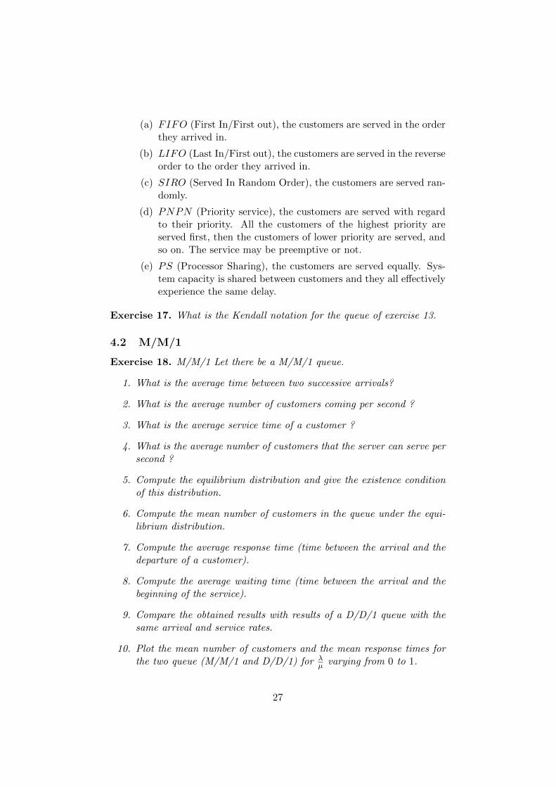
Number of customers Xt for a D/D/1 queueNumber of customers Xt for a D/D/1 queue
1/µ 1/µ 1/µ
0
1
The customers arrive at regular intervals.
1/λ 1/λ 1/λ
(a) The number of customers in the D/D/1queue
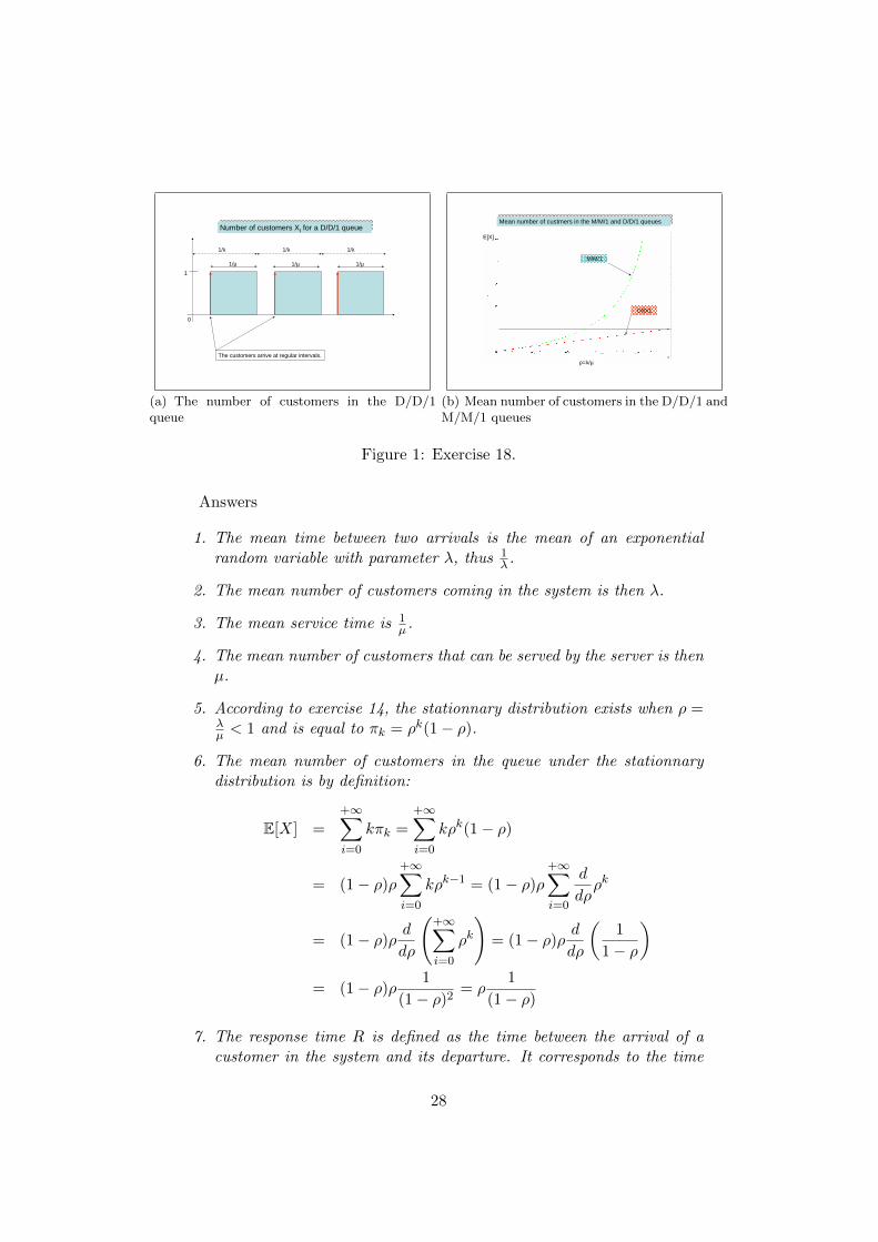
ρ=λ/µ1
Mean number of custmers in the M/M/1 and D/D/1 queuesMean number of custmers in the M/M/1 and D/D/1 queues
E[X]
M/M/1
D/D/1
(b) Mean number of customers in the D/D/1 andM/M/1 queues
Figure 1: Exercise 18.
Answers
1. The mean time between two arrivals is the mean of an exponentialrandom variable with parameter λ, thus 1
λ .
2. The mean number of customers coming in the system is then λ.
3. The mean service time is 1µ .
4. The mean number of customers that can be served by the server is thenµ.
5. According to exercise 14, the stationnary distribution exists when ρ =λµ < 1 and is equal to πk = ρk(1− ρ).
6. The mean number of customers in the queue under the stationnarydistribution is by definition:
E[X] =+∞∑i=0
kπk =+∞∑i=0
kρk(1− ρ)
= (1− ρ)ρ
+∞∑i=0
kρk−1 = (1− ρ)ρ
+∞∑i=0
d
dρρk
= (1− ρ)ρd
dρ
(+∞∑i=0
ρk
)= (1− ρ)ρ
d
dρ
(1
1− ρ
)= (1− ρ)ρ
1
(1− ρ)2= ρ
1
(1− ρ)
7. The response time R is defined as the time between the arrival of acustomer in the system and its departure. It corresponds to the time
28
spent in the system (time to queue and time in the server). To computethe mean response time, we use the result of exercise 26: E[X] =λE[R]. For the M/M/1 queue, the result is thus
E[R] =E[X]
λ=
ρ
λ(1− ρ)
8. The waiting time W is defined as the time that the customer spentin the system before being served. The mean waiting time is thus thedifference between the mean response time and the mean service time:
E[W ] = E[R]− 1
µ
9. The D/D/1 queue is a queue where both interarrivals and service timeare constant. Since, the arrival rate and service time are the same inaverage, we suppose that a server will serve a customer in a time equalto 1
µ and that the customers arrive at regular interval equal to 1λ . If we
suppose that λ < µ, the service time is less than the interarrival. Thenumber of customers varies from 0 to 1 as shown in Figure 1(a). Theprobability π1 that there is one customer in the system is then the ratio1µ1λ
= ρ (with ρ = λµ) and the probability π0 that there is no customer is
1 − ρ. The mean number of customers is then E[X] = 0π0 + 1π1 = ρand E[R] = 1
µ .
10. In Figure 1(b), we plot the mean number of customers E[X] for thetwo queues when ρ varies from 0 to 1. For the D/D/1 queue, E[X]tend to 1. For the M/M/1 queue, E[X] tends to infinity as ρ→ 1. So,for the second case, even if the arrival rate is less than service rate, therandomness of the interarrivals and service times leads to an explosionof the number of customers when the system is close to saturation.
4.3 M/M/K
Exercise 19. M/M/K Let there be a M/M/K queue.
1. Compute the equilibrium distribution and give the existence conditionof this distribution.
2. Compute the mean number of customers in the queue under the equi-librium distribution.
3. Compute the average response time.
4. Compute the average waiting time.
29
4.4 M/M/+∞
Exercise 20. M/M/+∞ Let there be a M/M/+∞ queue.
1. Compute the equilibrium distribution and give the existence conditionof this distribution.
2. Compute the mean number of customers in the queue under the equi-librium distribution.
3. Compute the average response time.
4. Compute the average waiting time.
4.5 M/M/K/K+C
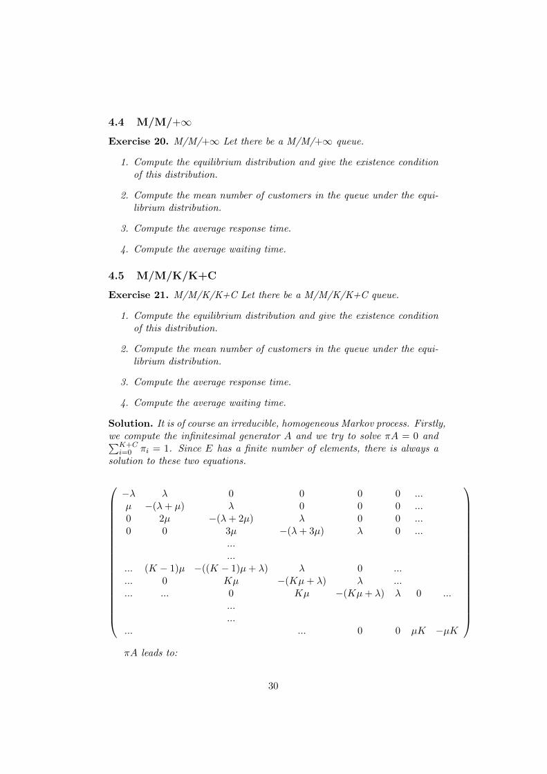
Exercise 21. M/M/K/K+C Let there be a M/M/K/K+C queue.
1. Compute the equilibrium distribution and give the existence conditionof this distribution.
2. Compute the mean number of customers in the queue under the equi-librium distribution.
3. Compute the average response time.
4. Compute the average waiting time.
Solution. It is of course an irreducible, homogeneous Markov process. Firstly,we compute the infinitesimal generator A and we try to solve πA = 0 and∑K+C
i=0 πi = 1. Since E has a finite number of elements, there is always asolution to these two equations.
−λ λ 0 0 0 0 ...µ −(λ+ µ) λ 0 0 0 ...0 2µ −(λ+ 2µ) λ 0 0 ...0 0 3µ −(λ+ 3µ) λ 0 ...
...
...... (K − 1)µ −((K − 1)µ+ λ) λ 0 ...... 0 Kµ −(Kµ+ λ) λ ...... ... 0 Kµ −(Kµ+ λ) λ 0 ...
...
...... ... 0 0 µK −µK
πA leads to:
30
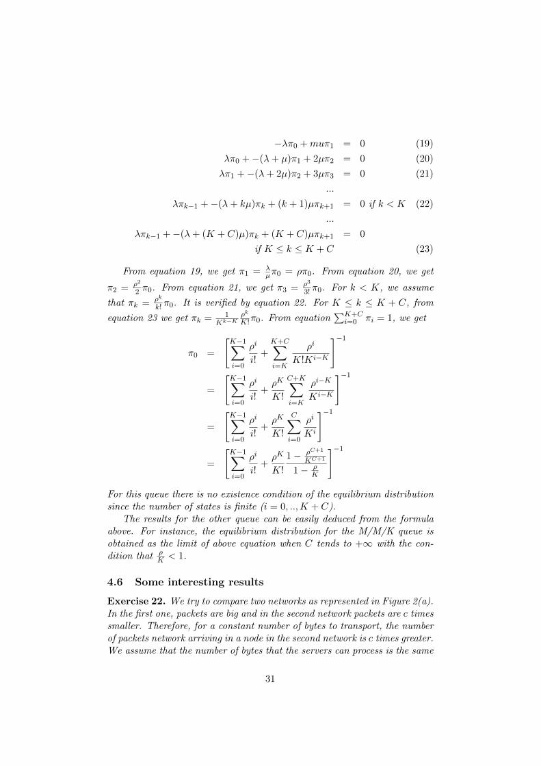
−λπ0 +muπ1 = 0 (19)
λπ0 +−(λ+ µ)π1 + 2µπ2 = 0 (20)
λπ1 +−(λ+ 2µ)π2 + 3µπ3 = 0 (21)
...
λπk−1 +−(λ+ kµ)πk + (k + 1)µπk+1 = 0 if k < K (22)
...
λπk−1 +−(λ+ (K + C)µ)πk + (K + C)µπk+1 = 0
if K ≤ k ≤ K + C (23)
From equation 19, we get π1 = λµπ0 = ρπ0. From equation 20, we get
π2 = ρ2
2 π0. From equation 21, we get π3 = ρ3
3! π0. For k < K, we assume
that πk = ρk
k! π0. It is verified by equation 22. For K ≤ k ≤ K + C, from
equation 23 we get πk = 1Kk−K
ρk
K!π0. From equation∑K+C
i=0 πi = 1, we get
π0 =
[K−1∑i=0
ρi
i!+K+C∑i=K
ρi
K!Ki−K
]−1
=
[K−1∑i=0
ρi
i!+ρK
K!
C+K∑i=K
ρi−K
Ki−K
]−1
=
[K−1∑i=0
ρi
i!+ρK
K!
C∑i=0
ρi
Ki
]−1
=
[K−1∑i=0
ρi
i!+ρK
K!
1− ρC+1
KC+1
1− ρK
]−1
For this queue there is no existence condition of the equilibrium distributionsince the number of states is finite (i = 0, ..,K + C).
The results for the other queue can be easily deduced from the formulaabove. For instance, the equilibrium distribution for the M/M/K queue isobtained as the limit of above equation when C tends to +∞ with the con-dition that ρ
K < 1.
4.6 Some interesting results
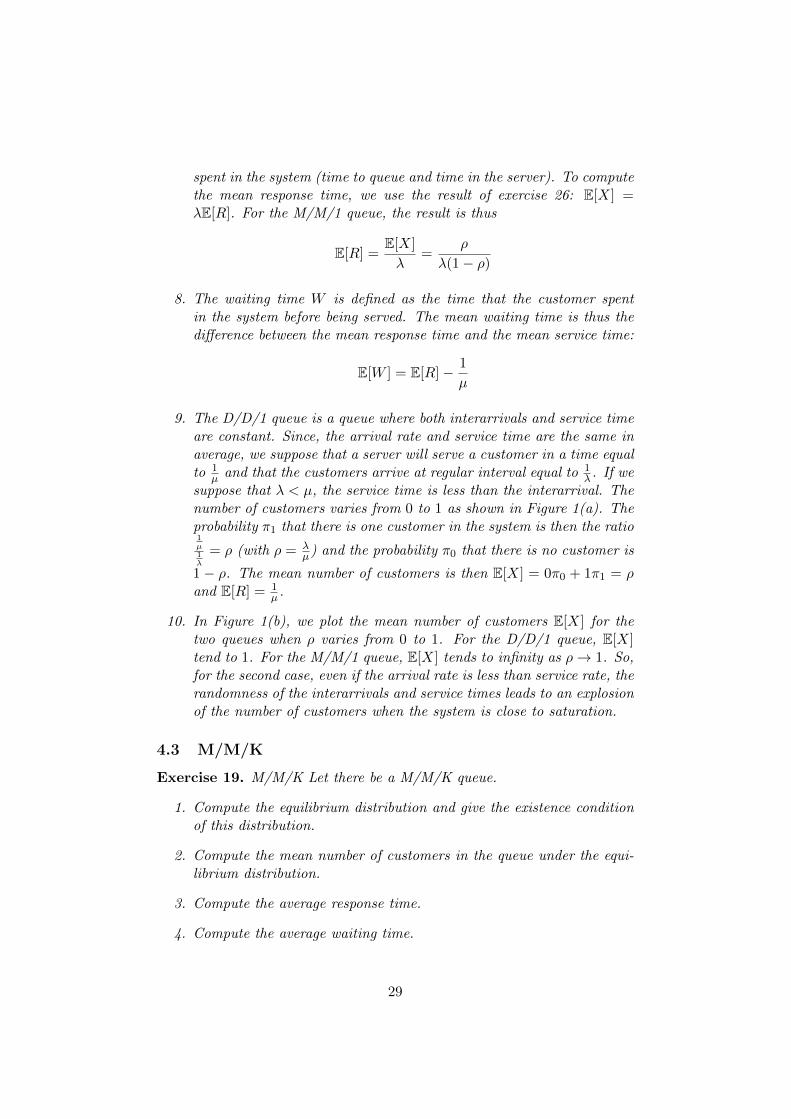
Exercise 22. We try to compare two networks as represented in Figure 2(a).In the first one, packets are big and in the second network packets are c timessmaller. Therefore, for a constant number of bytes to transport, the numberof packets network arriving in a node in the second network is c times greater.We assume that the number of bytes that the servers can process is the same
31

λ
μ
cλ
cμ
M/M/1
M/M/1
System 1System 1
System 3System 3System 2System 2
(a) Exercise 22
2 M/M/1
λ/2
λ/2
λ μ
μ
λ μ
μ
λ
2 μ
M/M/2
M/M/1
System 1
System 2System 2
System 3System 3
System 1System 1
System 3System 3
(b) Exercise 23
Figure 2: Comparison of different queues
for the two networks. So, servers in network B can process c times as manypackets.
The mathematical model is as follows We consider two M/M/1 queuescalled A and B corresponding to each network. The arrival rate of A is λ,and it is λc (with c > 1) for B. The service rate is µ for queue A, and µcfor queue B.
1. Compare the mean number of customers in the two queues.
2. Compare the average response time in the two queues.
3. If the average packet size in network A is L bytes, and Lc bytes in
network B, compute the mean number of bytes that the packets occupyin the node.
4. Conclude.
Solution. For queue A (ρ = λµ):
E[X] =ρ
1− ρand E[R] =
1
µ
ρ
1− ρ
For queue B:
E[X] =ρ
1− ρand E[R] =
1
cµ
ρ
1− ρ
So, in the second case (B) where packets are c times smaller, the meannumber of packets in the queue are the same. It is however more efficientbecause these packets are c times smaller and thus will take c times lessmemory in the node. The response time is then also shorter (since the
32
server capacity is constant), and is c times smaller than in queue A. Thereason for this difference, is variance. The variance increases with packetsize (for exponential law).
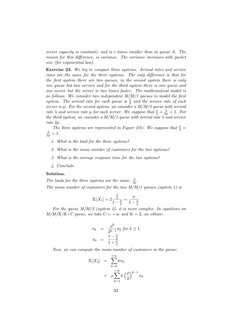
Exercise 23. We try to compare three systems. Arrival rates and servicerates are the same for the three systems. The only difference is that forthe first system there are two queues, in the second system there is onlyone queue but two servers and for the third system there is one queue andone server but the server is two times faster. The mathematical model isas follows. We consider two independent M/M/1 queues to model the firstsystem. The arrival rate for each queue is λ
2 and the service rate of eachserver is µ. For the second system, we consider a M/M/2 queue with arrivalrate λ and service rate µ for each server. We suppose that ρ
2 = λ2µ < 1. For
the third system, we consider a M/M/1 queue with arrival rate λ and servicerate 2µ.
The three systems are represented in Figure 2(b). We suppose that ρ2 =
λ2µ < 1.
1. What is the load for the three systems?
2. What is the mean number of customers for the two systems?
3. What is the average response time for the two systems?
4. Conclude.
Solution.
The loads for the three systems are the same: λ2µ .
The mean number of customers for the two M/M/1 queues (system 1) is
E [X1] = 2ρ2
1− ρ2
=ρ
1− ρ2
For the queue M/M/2 (system 2), it is more complex. In equations onM/M/K/K+C queue, we take C = +∞ and K = 2, we obtain:
πk =ρk
2k−1π0 for k ≥ 1
π0 =1− ρ
2
1 + ρ2
Now, we can compute the mean number of customers in the queue:
E [X2] =+∞∑k=0
kπk
= ρ
+∞∑k=1
k(ρ
2
)k−1π0
33

If x is real ∈]0, 1[, we get (to prove that, we have to consider that kxk−1
is the derivative of xk):
+∞∑k=1
kxk−1 =1
(1− x)2
With x = ρ2 , we get:
E [X2] = ρ+∞∑k=1
k(ρ
2
)k−1π0
=ρ
(1− ρ2)2
π0
=ρ
(1− ρ2)2
1− ρ2
1 + ρ2
=ρ
(1− ρ2)(1 + ρ
2)
For the third system (M/M/1), we obtain:
E [X3] =ρ2
1− ρ2
It appears that the mean number of customers is greater in system 1 and2: E[X1] > E[X2] > E[X3]. It is due to the fact that in system 1, withthe two M/M/1 queues, when one server is empty and the other queue hassome customers, the first one is not use leading to the waste of a part ofthe capacity. Moreover, the variance of the interarrival and service time isreally smaller for system 3 leading to better performances.
4.7 M/GI/1 and GI/M/1
When interarrival or service time is not exponential, the process describingthe number of customers is no more Markovian. The jump chain taken ateach jump of the process is not a Markov chain. However, for M/GI/1 andGI/M/1 we can build a Markov chain from the Markov process. These jumpchains are those defined in Section 3.2.
Exercise 24. 1. Prove that the jump chain taken at the arrival time ofa GI/M/1 is a Markov chain.
2. Prove that the jump chain taken at the departure time of a M/GI/1 isa Markov chain.
Solution. For the M/GI/1, we have to prove that
P (Xn = j|Xn−1 = in−1, ..., X0 = i0) = P(XS−n
= j|XS−n−1= in−1, ..., XS−0
= i0
)34

Since the interarrival process is a sequence of i.i.d. exponential r.v., it ismemory less. Thus the number of customers coming between S−n−1 and S−nis independent of the past. Moreover, there is only one service between S−n−1and S−n (it is not cut), its duration is independent of the past since servicetimes are independently distributed. Therefore, the probability that the chainchanges from state i to state j depends only on i and j. Therefore, it is aMarkov chain.
For the M/GI/1 and GI/M/1 queues, the transition probabilities dependon the considered ”GI” distribution. For instance, for M/GI/1 queue, fromstate j there is a positive probability to go to state j − 1 if no customerarrives between the two departures (between Xn−1 and Xn) and positiveprobabilities to go to state j + k if k customers arrive during the service ofthe customer currently in the server (between Xn−1 and Xn).
Exercise 25. We consider the M/D/1 and D/M/1 queues.
1. Compute the transition matrix of the jump chains for these two queues.
2. Compute the equilibrium distribution for the two queues. What are theexistence conditions?
3. Compute the mean number of customers and the mean response time.
Proposition 6. Khintchin-Pollazcek formula. The mean number of cus-tomers X in a M/GI/1 queue is
E[X] = ρ+ρ2(
1 + var(Y )E[Y ]2
)2(1− ρ)
where Y is a random variable with the same distribution as the service timeof a customer and ρ = λ
µ .
5 Miscellaneous
Exercise 26. We consider two moving walkways. The first one has a con-stant speed equal to 11km/h and the second 3km/h. Both moving walkwayshave a length of 500 meters. We also assume that there is a person arrivingon each moving walkway each second.
• Give the number of persons on each walkway.
• Deduce a formula which links the number of customers in a system,the mean arrival rate and the response time.
35