9 markov chains and hidden markov models - freie … · 9 markov chains and hidden markov models we...

9 Markov chains and Hidden Markov Models

We will discuss:

• Markov chains

• Hidden Markov Models (HMMs)

• Algorithms: Viterbi, forward, backward, posterior decoding

• Profile HMMs

• Baum-Welch algorithm

This chapter is based on:

• R. Durbin, S. Eddy, A. Krogh, G. Mitchison: Biological sequence analysis. Cambridge University Press,1998. ISBN 0-521-62971-3 (Chapter 3)

• An earlier version of this lecture by Daniel Huson.

• Lecture notes by Mario Stanke, 2006.

9.1 CpG-islands

As an introduction to Markov chains, we consider the problem of finding CpG-islands in the human genome.

A piece of double stranded DNA:...ApCpCpApTpGpApTpGpCpApGpGpApCpTpTpCpCpApTpCpGpTpTpCpGpCpGp...

...| | | | | | | | | | | | | | | | | | | | | | | | | | | | | ...

...TpGpGpTpApCpTpApCpGpTpCpCpTpGpApApGpGpTpApGpCpApApGpCpGpCp...

The C in a CpG pair is often modified by methylation (that is, an H-atom is replaced by a CH3-group). Thereis a relatively high chance that the methyl-C will mutate to a T. Hence, CpG-pairs are underrepresented in thehuman genome.

Methylation plays an important role in transscription regulation. Upstream of a gene, the methylationprocess is suppressed in a short region of length 100-5000. These areas are called CpG-islands. They arecharacterized by the fact that we see more CpG-pairs in them than elsewhere.

ThereforeCpG-islands are useful markers for genes in organisms whose genomes contain 5-methyl-cytosine.

CpG-islands in the promoter-regions of genes play an important role in the deactivation of one copy of theX-chromosome in females, in genetic imprinting and in the deactivation of intra-genomic parasites.

Classical definition: DNA sequence of length 200 with a C + G content of 50% and a ratio of observed-to-expected number of CpG’s that is above 0.6. (Gardiner-Garden & Frommer, 1987)

According to a recent study, human chromosomes 21 and 22 contain about 1100 CpG-islands and about 750genes. (Comprehensive analysis of CpG islands in human chromosomes 21 and 22, D. Takai & P. A. Jones, PNAS, March19, 2002)

Hidden Markov Models, by Clemens GrAPpl, January 23, 2014, 15:40 9001

More specifically, we can ask the following

Questions.

1. Given a (short) segment of genomic sequence.How to decide whether this segment is from a CpG-island or not?

2. Given a (long) segment of genomic sequence.How to find all CpG-islands contained in it?

9.2 Markov chains

Our goal is to come up with a probabilistic model for CpG-islands. Because pairs of consecutive nucleotides areimportant in this context, we need a model in which the probability of one symbol depends on the probabilityof its predecessor. This dependency is captured by the concept of a Markov chain.

Example.

A C

G T

• Circles = states, e.g. with names A, C, G and T.

• Arrows = possible transitions , each labeled with a transition probability ast. Let xi denote the state at timei. Then ast := P(xi+1 = t | xi = s) is the conditional probability to go to state t in the next step, given thatthe current state is s.

Definition.A (time-homogeneous) Markov chain (of order 1) is a system (Q,A) consisting of a finite set of states Q ={s1, s2, . . . , sn} and a transition matrix A = {ast} with

∑t∈Q ast = 1 for all s ∈ Q that determines the probability of

the transition s→ t byP(xi+1 = t | xi = s) = ast.

At any time i the Markov chain is in a specific state xi, and at the tick of a clock the chain changes to statexi+1 according to the given transition probabilities.

Remarks on terminology.

9002 Hidden Markov Models, by Clemens GrAPpl, January 23, 2014, 15:40

• Order 1 means that the transition probabilities of the Markov chain can only “remember” 1 state of itshistory. Beyond this, it is memoryless. The “memorylessness” condition is a very important. It is calledthe Markov property.

• The Markov chain is time-homogenous because the transition probability

P(xi+1 = t | xi = s) = ast.

does not depend on the time parameter i.

Example.Weather in Tubingen, daily at midday: Possible states are “rain”, “sun”, or “clouds”.

Transition probabilities:R S C

R .5 .1 .4S .2 .5 .3C .3 .3 .4

Note that all rows add up to 1.

Weather: ...rrrrrrccsssssscscscccrrcrcssss...

Given a sequence of states s1, s2, s3, . . . , sL. What is the probability that a Markov chain x = x1, x2, x3, . . . , xLwill step through precisely this sequence of states? We have

P(xL = sL, xL−1 = sL−1, . . . , x1 = s1)= P(xL = sL | xL−1 = sL−1, . . . , x1 = s1)· P(xL−1 = sL−1 | xL−2 = sL−2, . . . , x1 = s1)...

· P(x2 = s2 | x1 = s1)· P(x1 = s1)

using the “expansion”

P(A | B) =P(A ∩ B)

P(B)⇐⇒ P(A ∩ B) = P(A | B) · P(B) .

Now, we make use of the fact that

P(xi = si | xi−1 = si−1, . . . , x1 = s1) = P(xi = si | xi−1 = si−1)

by the Markov property. Thus

P(xL = sL, xL−1 = sL−1, . . . , x1 = s1)= P(xL = sL | xL−1 = sL − 1)· P(xL−1 = sL−1 | xL−2 = sL−2)· . . . · P(x2 = s2 | x1 = s1) · P(x1 = s1)

= P(x1 = s1)L∏

i=2

asi−1si .

Hence:

The probability of a path is the product of the probability of the initial state and the transitionprobabilities of its edges.


9.3 Modeling the begin and end states

A Markov chain starts in state x1 with an initial probability of P(x1 = s). For simplicity (i.e., uniformity of themodel) we would like to model this probability as a transition, too.

Therefore we add a begin state to the model that is labeled ’b’. We also impose the constraint that x0 = bholds. Then:

P(x1 = s) = abs .

This way, we can store all probabilities in one matrix and the “first” state x1 is no longer special:

P(xL = sL, xL−1 = sL−1, . . . , x1 = s1) =

L∏i=1

asi−1si .

Similarly, we explicitly model the end of the sequence of states using an end state ’e’. Thus, the probabilitythat the Markov chain stops is

P(xL = t) = axLe.

if the current state is t.

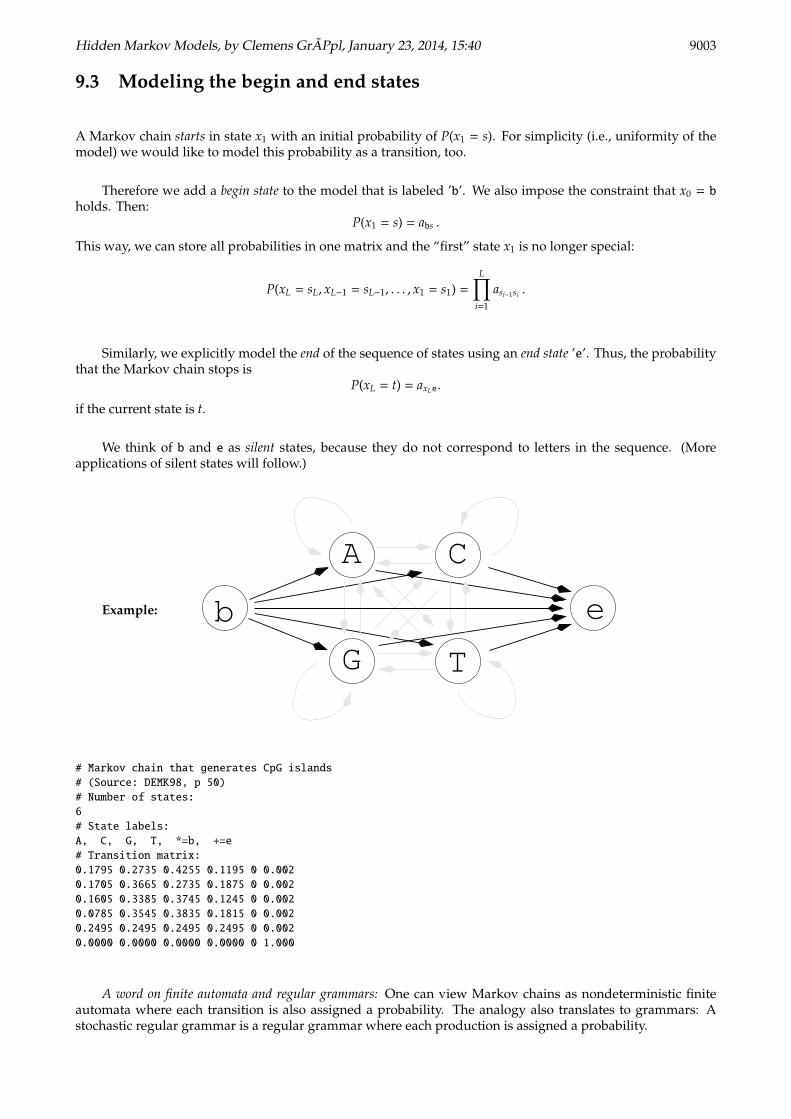
We think of b and e as silent states, because they do not correspond to letters in the sequence. (Moreapplications of silent states will follow.)

Example:

A C

G T

eb

# Markov chain that generates CpG islands

# (Source: DEMK98, p 50)

# Number of states:

6

# State labels:

A, C, G, T, *=b, +=e

# Transition matrix:

0.1795 0.2735 0.4255 0.1195 0 0.002

0.1705 0.3665 0.2735 0.1875 0 0.002

0.1605 0.3385 0.3745 0.1245 0 0.002

0.0785 0.3545 0.3835 0.1815 0 0.002

0.2495 0.2495 0.2495 0.2495 0 0.002

0.0000 0.0000 0.0000 0.0000 0 1.000

A word on finite automata and regular grammars: One can view Markov chains as nondeterministic finiteautomata where each transition is also assigned a probability. The analogy also translates to grammars: Astochastic regular grammar is a regular grammar where each production is assigned a probability.


9.4 Determining the transition matrix

How do we find transition probabilities that explain a given set of sequences best?

The transition matrix A+ for DNA that comes from a CpG-island, is determined as follows:

a+st =

c+st∑

t′ c+st′,

where cst is the number of positions in a training set of CpG-islands at which state s is followed by state t. Wecan calculate these counts in a single pass over the sequences and store them in a Σ × Σ matrix.

We obtain the matrix A− for non-CpG-islands from empirical data in a similar way.

In general, the matrix of transition probabilities is not symmetric.

Two examples of Markov chains.

# Markov chain for CpG islands # Markov chain for non-CpG islands

# (Source: DEMK98, p 50) # (Source: DEMK98, p 50)

# Number of states: # Number of states:

6 6

# State labels: # State labels:

A C G T * + A C G T * +

# Transition matrix: # Transition matrix:

.1795 .2735 .4255 .1195 0 0.002 .2995 .2045 .2845 .2095 0 .002

.1705 .3665 .2735 .1875 0 0.002 .3215 .2975 .0775 .3015 0 .002

.1605 .3385 .3745 .1245 0 0.002 .2475 .2455 .2975 .2075 0 .002

.0785 .3545 .3835 .1815 0 0.002 .1765 .2385 .2915 .2915 0 .002

.2495 .2495 .2495 .2495 0 0.002 .2495 .2495 .2495 .2495 0 .002

.0000 .0000 .0000 .0000 0 1.000 .0000 .0000 .0000 .0000 0 1.00

Note the different values for CpG: a+CG = 0.2735 versus a−CG = 0.0775.

9.5 Testing hypotheses

When we have two models, we can ask which one explains the observation better.

Given a (short) sequence x = (x1, x2, . . . , xL). Does it come from a CpG-island (model+)?

We have

P(x | model+) =

L∏i=0

a+xixi+1

,

with x0 = b and xL+1 = e. Similar for (model−).

To compare the models, we calculate the log-odds ratio:

S(x) = logP(x | model+)P(x | model−)

=

L∑i=0

loga+

xi−1xi

a−xi−1xi

.

Then this ratio is normalized by the length of x. This resulting length-normalized log-odds score S(x)/|x| canbe used to classify x. The higher this score is, the higher the probability is that x comes from a CpG-island.


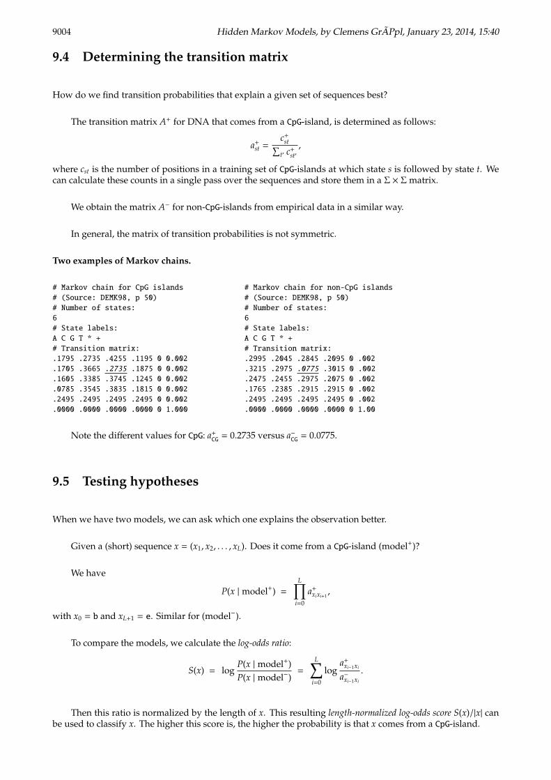
The histogram of the length-normalized scores for the sequences from the training sets for A+ and A−

shows that S(x)/|x| is indeed a good classifier for this data set. (Since the base two logarithm was used, the unitof measurement is called “bits”.)

Example.Weather in Tubingen, daily at midday: Possible states are rain, sun or clouds.

Types of questions that the Markov chain model can answer:

If it is sunny today, what is the probability that the sun will shine for the next seven days?

And what is more unlikely: 7 days sun or 8 days rain?

9.6 Hidden Markov Models (HMMs)

Motivation: Question 2, how to find CpG-islands in a long sequence?

We could approach this using Markov Chains and a “window technique”: a window of width w is movedalong the sequence and the score (as defined above) is plotted. However the results are somewhat unsatifactory:It is hard to determine the boundaries of CpG-islands, and which window size w should one choose? . . .

The basic idea is to relax the tight connection between “states” and “symbols”. Instead, every state can“emit” every symbol. There is an emission probability ek(b) for each state k and symbol b.

However, when we do so, we no longer know for sure the state from which an observed symbol wasemitted. In this sense, the Markov model is hidden; hence the name.

Definition.Am HMM is a system M = (Σ,Q,A, e) consisting of

• an alphabet Σ,

• a set of states Q,


• a matrix A = {akl} of transition probabilities akl for k, l ∈ Q, and

• an emission probability ek(b) for every k ∈ Q and b ∈ Σ.

9.7 HMM for CpG-islands

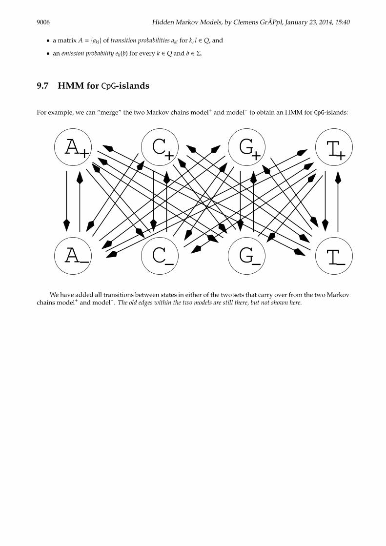
For example, we can “merge” the two Markov chains model+ and model− to obtain an HMM for CpG-islands:

A C TG

A C TG+ + + +

− − − −

We have added all transitions between states in either of the two sets that carry over from the two Markovchains model+ and model−. The old edges within the two models are still there, but not shown here.


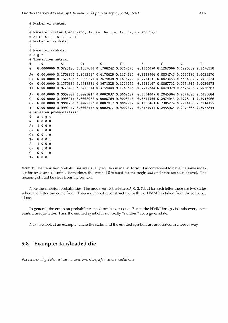
# Number of states:

9

# Names of states (begin/end, A+, C+, G+, T+, A-, C-, G- and T-):

0 A+ C+ G+ T+ A- C- G- T-

# Number of symbols:

4

# Names of symbols:

a c g t

# Transition matrix:

# 0 A+ C+ G+ T+ A- C- G- T-

0 0.0000000 0.0725193 0.1637630 0.1788242 0.0754545 0.1322050 0.1267006 0.1226380 0.1278950

A+ 0.0010000 0.1762237 0.2682517 0.4170629 0.1174825 0.0035964 0.0054745 0.0085104 0.0023976

C+ 0.0010000 0.1672435 0.3599201 0.2679840 0.1838722 0.0034131 0.0073453 0.0054690 0.0037524

G+ 0.0010000 0.1576223 0.3318881 0.3671328 0.1223776 0.0032167 0.0067732 0.0074915 0.0024975

T+ 0.0010000 0.0773426 0.3475514 0.3759440 0.1781818 0.0015784 0.0070929 0.0076723 0.0036363

A- 0.0010000 0.0002997 0.0002047 0.0002837 0.0002097 0.2994005 0.2045904 0.2844305 0.2095804

C- 0.0010000 0.0003216 0.0002977 0.0000769 0.0003016 0.3213566 0.2974045 0.0778441 0.3013966

G- 0.0010000 0.0001768 0.0002387 0.0002917 0.0002917 0.1766463 0.2385224 0.2914165 0.2914155

T- 0.0010000 0.0002477 0.0002457 0.0002977 0.0002077 0.2475044 0.2455084 0.2974035 0.2075844

# Emission probabilities:

# a c g t

0 0 0 0 0

A+ 1 0 0 0

C+ 0 1 0 0

G+ 0 0 1 0

T+ 0 0 0 1

A- 1 0 0 0

C- 0 1 0 0

G- 0 0 1 0

T- 0 0 0 1

Remark: The transition probabilities are usually written in matrix form. It is convenient to have the same indexset for rows and columns. Sometimes the symbol 0 is used for the begin and end state (as seen above). Themeaning should be clear from the context.

Note the emission probabilities: The model emits the letters A, C, G, T, but for each letter there are two stateswhere the letter can come from. Thus we cannot reconstruct the path the HMM has taken from the sequencealone.

In general, the emission probabilities need not be zero-one. But in the HMM for CpG-islands every stateemits a unique letter. Thus the emitted symbol is not really “random” for a given state.

Next we look at an example where the states and the emitted symbols are associated in a looser way.

9.8 Example: fair/loaded die

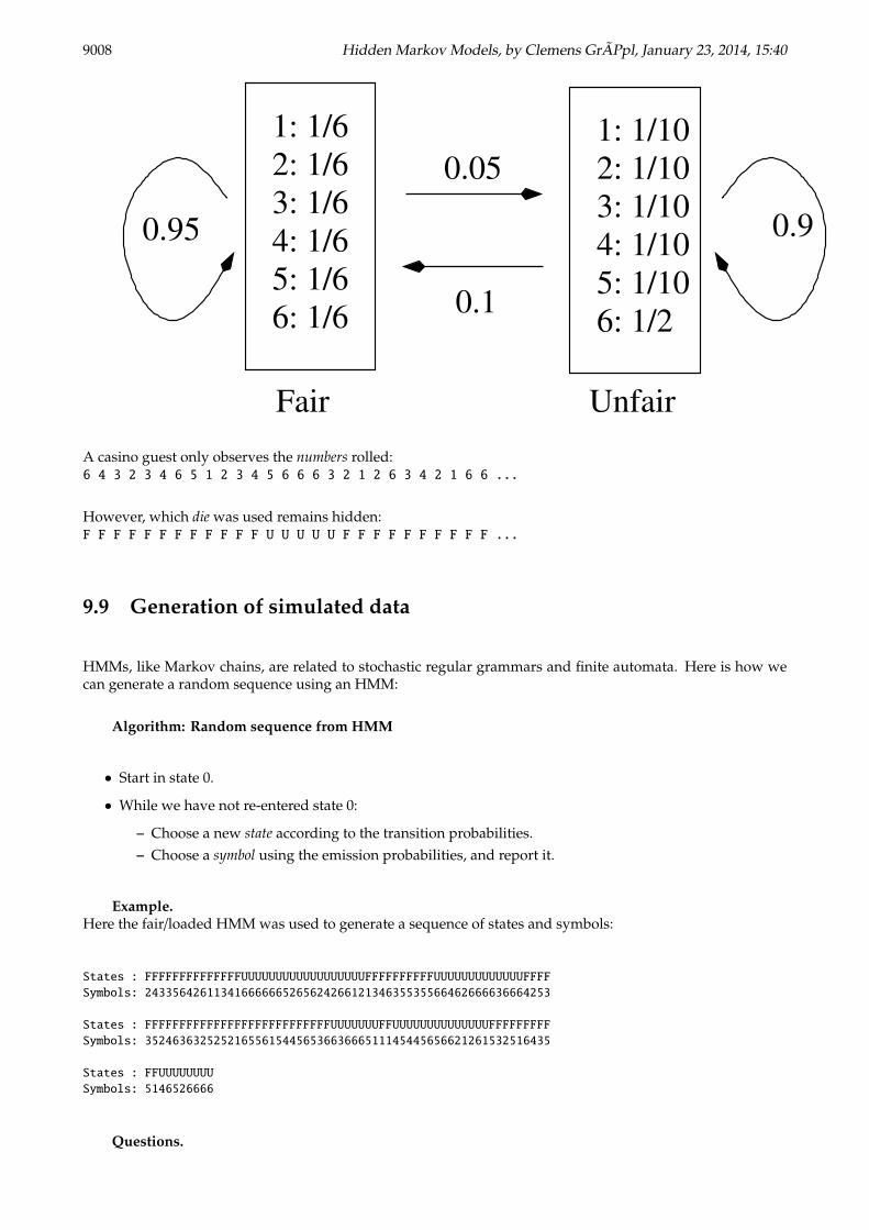
An occasionally dishonest casino uses two dice, a fair and a loaded one:


1: 1/62: 1/63: 1/64: 1/65: 1/66: 1/6

1: 1/102: 1/103: 1/104: 1/105: 1/106: 1/2

0.05

0.1

0.95 0.9

UnfairFairA casino guest only observes the numbers rolled:6 4 3 2 3 4 6 5 1 2 3 4 5 6 6 6 3 2 1 2 6 3 4 2 1 6 6 ...

However, which die was used remains hidden:F F F F F F F F F F F F U U U U U F F F F F F F F F F ...

9.9 Generation of simulated data

HMMs, like Markov chains, are related to stochastic regular grammars and finite automata. Here is how wecan generate a random sequence using an HMM:

Algorithm: Random sequence from HMM

• Start in state 0.

• While we have not re-entered state 0:

– Choose a new state according to the transition probabilities.– Choose a symbol using the emission probabilities, and report it.

Example.Here the fair/loaded HMM was used to generate a sequence of states and symbols:

States : FFFFFFFFFFFFFFUUUUUUUUUUUUUUUUUUFFFFFFFFFFUUUUUUUUUUUUUFFFF

Symbols: 24335642611341666666526562426612134635535566462666636664253

States : FFFFFFFFFFFFFFFFFFFFFFFFFFFUUUUUUUFFUUUUUUUUUUUUUUFFFFFFFFF

Symbols: 35246363252521655615445653663666511145445656621261532516435

States : FFUUUUUUUU

Symbols: 5146526666

Questions.


• Given an HMM and a sequence of states and symbols. What is the probability to get this sequence?

• Given an HMM and a sequence of symbols. Can we reconstruct the corresponding sequence of states,assuming that the sequence was generated using the HMM?

9.10 Probability for given states and symbols

Definitions.

• A path π = (π1, π2, . . . , πL) in an HMM M = (Σ,Q,A, e) is a sequence of states πi ∈ Q.

• Given a sequence of symbols x = (x1, . . . , xL) and a pathπ = (π1, . . . , πL) through M. Then the joint probabilityis:

P(x, π) = a0π1

L∏i=1

eπi (xi)aπiπi+1 ,

with πL+1 = 0.

Schematically,begin→

transitiona0,π1

→emissioneπ1 (x1)

→transition

aπ1 ,π2→

emissioneπ2 (x2)

→ · · · →transition

aπL ,0→ end

All we need to do is multiply these probabilities .

This answers the first question. However, usually we do not know the path π through the model! Thatinformation is hidden.

9.11 The decoding problem

The decoding problem is the following: We have observed a sequence x of symbols that was generated by anHMM and we would like to “decode” the sequence of states from it.

Example: The sequence of symbols CGCG has a large number of possible “explanations” within the CpG-model, including e.g.:

(C+,G+,C+,G+), (C−,G−,C−,G−) and (C−,G+,C−,G+).

Among these, the first one is more likely than the second. The third one is very unlikely because the“signs” alternate, and those transitions have small probabilities.

A path through the HMM determines which parts of the sequence x are classified as CpG-islands (+/−).Such a classification of the observed symbols is also called a decoding. But here we will only consider the casewhere we want to reconstruct the passed states themselves, and not a “projection” of them.

Another example.In speech recognition, HMMs have been applied since the 1970s. One application is the following. A speechsignal is sliced into pieces of 10-20 milliseconds, each of which is assigned to one of e.g. 256 categories. Wewant to find out what sequence of phonemes was spoken. Since the pronounciation of phonemes in naturallanguage varies a lot, we are faced with a decoding problem.


The most probable path. To solve the decoding problem, we want to determine the pathπ∗ that maximizesthe probability of having generated the sequence x of symbols, that is:

π∗ = arg maxπ

Pr(π | x) = arg maxπ

Pr(π, x).

For a sequence of n symbols there are |Q|n possible paths, therefore we cannot solve the problem by fullenumeration.

Luckily, the “most probable path” π∗ can be computed by dynamic programming. The recursion involvesthe following entities:

Definition. Given a prefix (x1, x2, . . . , xi) of the sequence x which is to be decoded. Then let (π∗1, π∗

2, . . . , π∗

i )be a path of states with π∗i = s which maximizes the probability that the HMM followed theses states and emittedthe symbols (x1, x2, . . . , xi) along its way. That is,

(π∗1, . . . , π∗

i ) = arg max{ i∏

k=1

aπi−1,πi eπi (xi)∣∣∣∣ (π1, . . . , πi) ∈ Qi, πi = s, π0 = 0

}.

Also, let V(s, i) denote the value of this maximal probability. These are sometimes called Viterbi variables.

Clearly we can store the values V(s, i) in a Q × [1 .. L] dynamic programming matrix.

Initialization.Every path starts at state 0 with probability 1. Hence, the initialization for i = 0 is V(0, 0) = 1, and V(s, 0) = 0 fors ∈ Q \ {0}.

Recursion.Now for the recurrence formula, which applies for i = 1, . . . ,L. Assume that we know the most likely path forx1, . . . , xi−1 under the additional constraint that the last state is s, for all s ∈ Q. Then we obtain the most likelypath to the i-th state t by maximizing the probability V(s, i − 1)ast over all predecessors s ∈ Q of t. To obtainV(t, i) we also have to multiply by et(xi) since we have to emit the given symbol xi.

That is, we haveV(t, i) = max{ V(s, i − 1)ast | s ∈ Q } · et(xi)

for all t ∈ Q. (Again, note the use of the Markov property!)

Termination.In the last step, we enter state 0 but do not emit a symbol. Hence P(x, π∗) = max{ V(s,L)as,0 | s ∈ Q }.


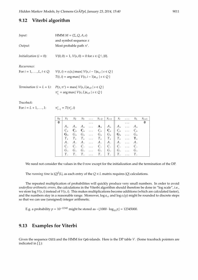
9.12 Viterbi algorithm

Input: HMM M = (Σ,Q,A, e)

and symbol sequence x

Output: Most probable path π∗.

Initialization (i = 0): V(0, 0) = 1, V(s, 0) = 0 for s ∈ Q \ {0}.

Recurrence:

For i = 1, . . . ,L, t ∈ Q: V(t, i) = et(xi) max{ V(s, i − 1)as,t | s ∈ Q }

T(t, i) = arg max{ V(s, i − 1)as,t | s ∈ Q }

Termination (i = L + 1): P(x, π∗) = max{ V(s,L)as,0 | s ∈ Q }

π∗L = arg max{ V(s,L)as,0 | s ∈ Q }

Traceback:

For i = L + 1, . . . , 1: π∗i−1 = T(π∗i , i)

x0 x1 x2 x3 . . . xi−2 xi−1 xi . . . xL xL+1

0 . . . . . . 0A+ A+ A+ . . . A+ A+ A+ . . . A+

C+ C+ C+ . . . C+ C+ C+ . . . C+

G+ G+ G+ . . . G+ G+ G+ . . . G+

T+ T+ T+ . . . T+ T+ T+ . . . T+

A− A− A− . . . A− A− A− . . . A−C− C− C− . . . C− C− C− . . . C−G− G− G− . . . G− G− G− . . . G−T− T− T− . . . T− T− T− . . . T−

We need not consider the values in the 0 row except for the initialization and the termination of the DP.

The running time is |Q|2|L|, as each entry of the Q × L matrix requires |Q| calculations.

The repeated multiplication of probabilities will quickly produce very small numbers. In order to avoidunderflow arithmetic errors, the calculations in the Viterbi algorithm should therefore be done in “log scale”, i.e.,we store log V(s, i) instead of V(s, i). This makes multiplications become additions (which are calculated faster),and the numbers stay in a reasonable range. Moreover, log as,t and log et(y) might be rounded to discrete stepsso that we can use (unsigned) integer arithmetic.

E.g. a probability p = 10−12345 might be stored as −b1000 · log10 pc = 12345000.

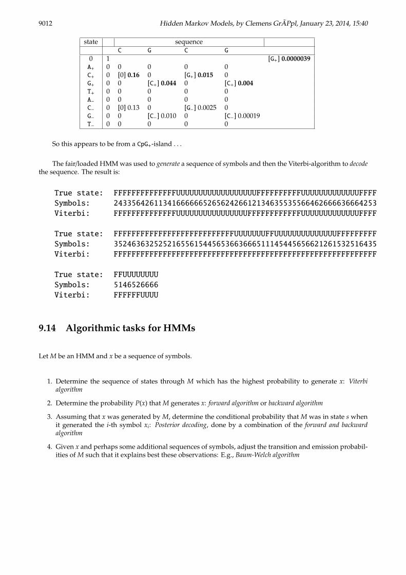
9.13 Examples for Viterbi

Given the sequence CGCG and the HMM for CpG-islands. Here is the DP table V. (Some traceback pointers areindicated in [ ].):


state sequenceC G C G

0 1 [G+] 0.0000039A+ 0 0 0 0 0C+ 0 [0] 0.16 0 [G+] 0.015 0G+ 0 0 [C+] 0.044 0 [C+] 0.004T+ 0 0 0 0 0A− 0 0 0 0 0C− 0 [0] 0.13 0 [G−] 0.0025 0G− 0 0 [C−] 0.010 0 [C−] 0.00019T− 0 0 0 0 0

So this appears to be from a CpG+-island . . .

The fair/loaded HMM was used to generate a sequence of symbols and then the Viterbi-algorithm to decodethe sequence. The result is:

True state: FFFFFFFFFFFFFFUUUUUUUUUUUUUUUUUUFFFFFFFFFFUUUUUUUUUUUUUFFFF

Symbols: 24335642611341666666526562426612134635535566462666636664253

Viterbi: FFFFFFFFFFFFFFUUUUUUUUUUUUUUUUFFFFFFFFFFFFUUUUUUUUUUUUUFFFF

True state: FFFFFFFFFFFFFFFFFFFFFFFFFFFUUUUUUUFFUUUUUUUUUUUUUUFFFFFFFFF

Symbols: 35246363252521655615445653663666511145445656621261532516435

Viterbi: FFFFFFFFFFFFFFFFFFFFFFFFFFFFFFFFFFFFFFFFFFFFFFFFFFFFFFFFFFF

True state: FFUUUUUUUU

Symbols: 5146526666

Viterbi: FFFFFFUUUU

9.14 Algorithmic tasks for HMMs

Let M be an HMM and x be a sequence of symbols.

1. Determine the sequence of states through M which has the highest probability to generate x: Viterbialgorithm

2. Determine the probability P(x) that M generates x: forward algorithm or backward algorithm

3. Assuming that x was generated by M, determine the conditional probability that M was in state s whenit generated the i-th symbol xi: Posterior decoding, done by a combination of the forward and backwardalgorithm

4. Given x and perhaps some additional sequences of symbols, adjust the transition and emission probabil-ities of M such that it explains best these observations: E.g., Baum-Welch algorithm


9.15 Forward algorithm

We have already seen a closed formula for the probability P(x, π) that M generated x using the pathπ. Summingover all possible paths, we obtain the probability that M generated x:

P(x) =∑π

P(x, π) .

Calculating this sum is done by “replacing the max with a sum” in the Viterbi algorithm.

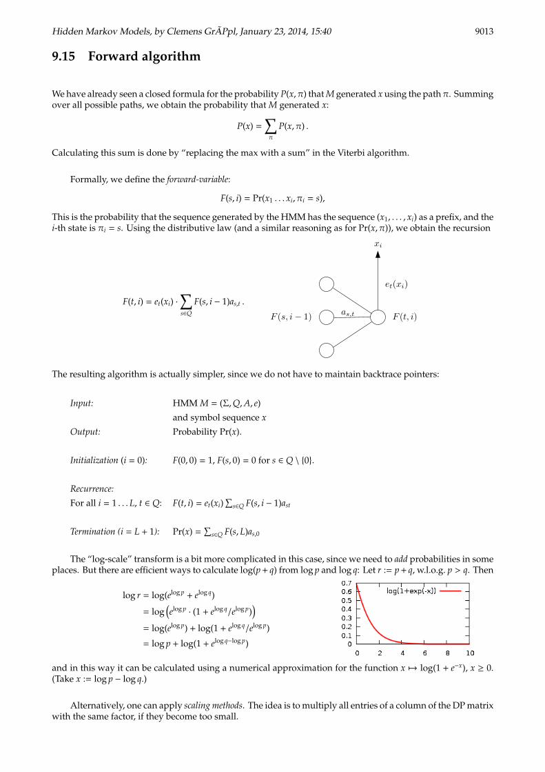
Formally, we define the forward-variable:

F(s, i) = Pr(x1 . . . xi, πi = s),

This is the probability that the sequence generated by the HMM has the sequence (x1, . . . , xi) as a prefix, and thei-th state is πi = s. Using the distributive law (and a similar reasoning as for Pr(x, π)), we obtain the recursion

F(t, i) = et(xi) ·∑s∈Q

F(s, i − 1)as,t .

F (t, i)F (s, i− 1)as,t

xi

et(xi)

The resulting algorithm is actually simpler, since we do not have to maintain backtrace pointers:



Output: Probability Pr(x).

Initialization (i = 0): F(0, 0) = 1, F(s, 0) = 0 for s ∈ Q \ {0}.

Recurrence:

For all i = 1 . . . L, t ∈ Q: F(t, i) = et(xi)∑

s∈Q F(s, i − 1)ast

Termination (i = L + 1): Pr(x) =∑

s∈Q F(s,L)as,0

The “log-scale” transform is a bit more complicated in this case, since we need to add probabilities in someplaces. But there are efficient ways to calculate log(p + q) from log p and log q: Let r := p + q, w.l.o.g. p > q. Then

log r = log(elog p + elog q)

= log(elog p

· (1 + elog q/elog p))

= log(elog p) + log(1 + elog q/elog p)

= log p + log(1 + elog q−log p)

and in this way it can be calculated using a numerical approximation for the function x 7→ log(1 + e−x), x ≥ 0.(Take x := log p − log q.)

Alternatively, one can apply scaling methods. The idea is to multiply all entries of a column of the DP matrixwith the same factor, if they become too small.


9.16 Backward algorithm

Recall the definition of the forward-variables:

F(s, i) = Pr(x1 . . . xi, πi = s) .

This is the probability that the sequence generated by the HMM has the sequence (x1, . . . , xi) as a prefix, and thei-th state is πi = s.

For the posterior decoding (described later) we need to compute the conditional probability that M emittedxi from state πi, when it happened to generate x:

Pr(πi = s | x) =Pr(πi = s, x)

Pr(x).

Since Pr(x) is known by the forward algorithm, it suffices to calculate Pr(πi = s, x). We have

Pr(x, πi = s) = Pr(x1, . . . , xi, πi = s) Pr(xi+1, . . . , xL | x1, . . . , xi, πi = s)= Pr(x1, . . . , xi, πi = s) Pr(xi+1, . . . , xL | πi = s) ,

using the Markov property in the second equation.

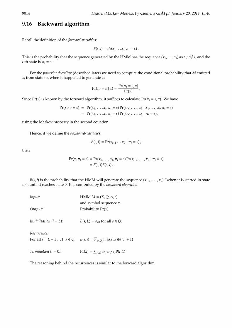
Hence, if we define the backward-variables:

B(s, i) = Pr(xi+1 . . . xL | πi = s) ,

then

Pr(x, πi = s) = Pr(x1, . . . , xi, πi = s) Pr(xi+1, . . . , xL | πi = s)= F(s, i)B(s, i) .

B(s, i) is the probability that the HMM will generate the sequence (xi+1, . . . , xL) “when it is started in stateπi”, until it reaches state 0. It is computed by the backward algorithm.



Output: Probability Pr(x).

Initialization (i = L): B(s,L) = as,0 for all s ∈ Q.

Recurrence:

For all i = L − 1 . . . 1, s ∈ Q: B(s, i) =∑

t∈Q astet(xi+1)B(t, i + 1)

Termination (i = 0): Pr(x) =∑

t∈Q a0,tet(x1)B(t, 1)

The reasoning behind the recurrences is similar to the forward algorithm.


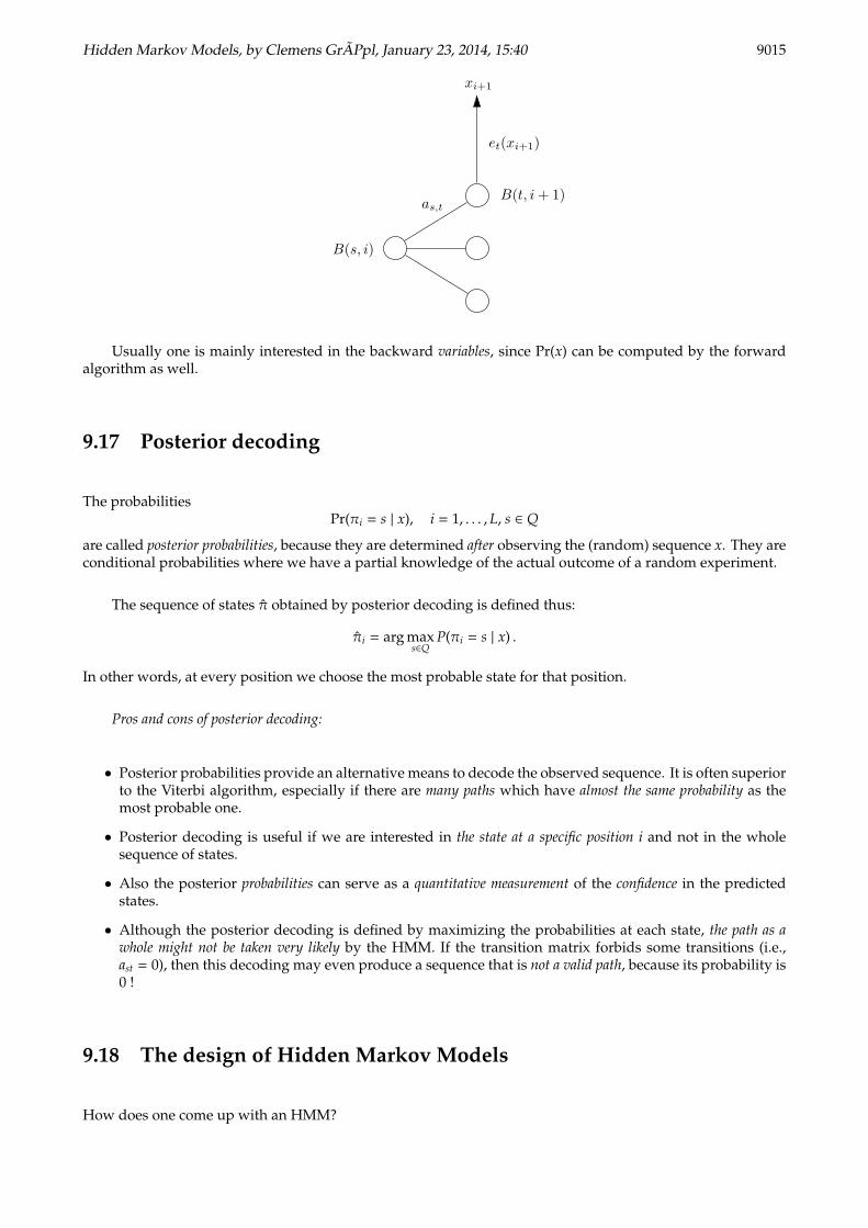
B(t, i+ 1)

B(s, i)

as,t

xi+1

et(xi+1)

Usually one is mainly interested in the backward variables, since Pr(x) can be computed by the forwardalgorithm as well.

9.17 Posterior decoding

The probabilitiesPr(πi = s | x), i = 1, . . . ,L, s ∈ Q

are called posterior probabilities, because they are determined after observing the (random) sequence x. They areconditional probabilities where we have a partial knowledge of the actual outcome of a random experiment.

The sequence of states π obtained by posterior decoding is defined thus:

πi = arg maxs∈Q

P(πi = s | x) .

In other words, at every position we choose the most probable state for that position.

Pros and cons of posterior decoding:

• Posterior probabilities provide an alternative means to decode the observed sequence. It is often superiorto the Viterbi algorithm, especially if there are many paths which have almost the same probability as themost probable one.

• Posterior decoding is useful if we are interested in the state at a specific position i and not in the wholesequence of states.

• Also the posterior probabilities can serve as a quantitative measurement of the confidence in the predictedstates.

• Although the posterior decoding is defined by maximizing the probabilities at each state, the path as awhole might not be taken very likely by the HMM. If the transition matrix forbids some transitions (i.e.,ast = 0), then this decoding may even produce a sequence that is not a valid path, because its probability is0 !

9.18 The design of Hidden Markov Models

How does one come up with an HMM?


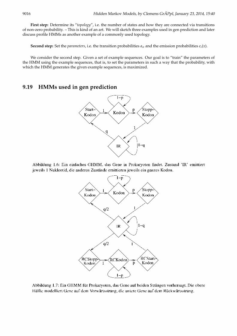
First step: Determine its “topology”, i.e. the number of states and how they are connected via transitionsof non-zero probability. – This is kind of an art. We will sketch three examples used in gen prediction and laterdiscuss profile HMMs as another example of a commonly used topology.

Second step: Set the parameters, i.e. the transition probabilities ast and the emission probabilities es(x).

We consider the second step. Given a set of example sequences. Our goal is to “train” the parameters ofthe HMM using the example sequences, that is, to set the parameters in such a way that the probability, withwhich the HMM generates the given example sequences, is maximized.

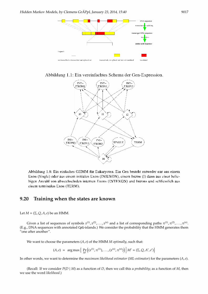
9.19 HMMs used in gen prediction


9.20 Training when the states are known

Let M = (Σ,Q,A, e) be an HMM.

Given a list of sequences of symbols x(1), x(2), . . . , x(n) and a list of corresponding paths π(1), π(2), . . . , π(n).(E.g., DNA sequences with annotated CpG-islands.) We consider the probability that the HMM generates them“one after another”.

We want to choose the parameters (A, e) of the HMM M optimally, such that:

(A, e) = arg max{

PrM′

((x(1), π(1)), . . . , (x(n), π(n))

) ∣∣∣∣ M′ = (Σ,Q,A′, e′)}

In other words, we want to determine the maximum likelihood estimator (ML-estimator) for the parameters (A, e).

(Recall: If we consider P(D | M) as a function of D, then we call this a probability; as a function of M, thenwe use the word likelihood.)


Not surprisingly, it turns out (analytically) that the likelihood is maximized by the estimators

Ast :=Ast∑t′ As,t′

and est :=est∑t′ es,t′

,

where

Ast := Observed number of transitions from state s to state t,esb := Observed number of emissions of symbol b in state s.

(However this presumes that we have sufficient training data.)

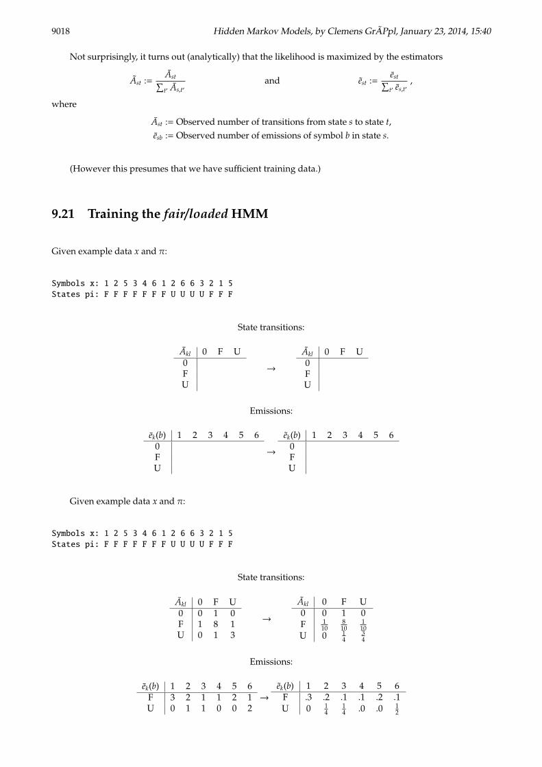
9.21 Training the fair/loaded HMM

Given example data x and π:

Symbols x: 1 2 5 3 4 6 1 2 6 6 3 2 1 5

States pi: F F F F F F F U U U U F F F

State transitions:

Akl 0 F U0FU

→

Akl 0 F U0FU

Emissions:

ek(b) 1 2 3 4 5 60FU

→

ek(b) 1 2 3 4 5 60FU

Given example data x and π:

Symbols x: 1 2 5 3 4 6 1 2 6 6 3 2 1 5

States pi: F F F F F F F U U U U F F F

State transitions:

Akl 0 F U0 0 1 0F 1 8 1U 0 1 3

→

Akl 0 F U0 0 1 0F 1

10810

110

U 0 14

34

Emissions:

ek(b) 1 2 3 4 5 6F 3 2 1 1 2 1U 0 1 1 0 0 2

→

ek(b) 1 2 3 4 5 6F .3 .2 .1 .1 .2 .1U 0 1

414 .0 .0 1

2


9.22 Pseudocounts

One common problem in training is overfitting. For example, if some possible transition (s, t) is never seen inthe example data, then we will set ast = 0 and the transition is then forbidden in the resulting HMM. Moreover,if a given state s is never seen in the example data, then ast resp. es(b) is undefined for all t, b.

To solve this problem, we introduce pseudocounts rst and rs(b) and add them to the observed transition resp.emission frequencies.

Small pseudocounts reflect “little pre-knowledge”, large ones reflect “more pre-knowledge”. The effect ofpseudocounts can also be thought of as “smoothing” the model parameters using a background model (i. e., aprior distribution).

9.23 Training when the states are unknown

Now we assume we are given a list of sequences of symbols x(1), x(2), . . . , x(n) and we do not know the list ofcorresponding paths π(1), π(2), . . . , π(n), as is usually the case in practice.

Then the problem to choose the parameters (A, e) of the HMM M optimally, such that:

(A, e) = arg max{

PrM′

(x(1), . . . , x(n)

) ∣∣∣∣ M′ = (Σ,Q,A′, e′)}

is NP-hard and hence we cannot be solve it exactly in polynomial time.

The quantity

log PrM′

(x(1), . . . , x(n)

)=

n∑j=1

log PrM′

(x( j)

)is called the log-likelihood of the model M.

It serves as a measure of the quality of the model parameters.

The Baum-Welch algorithm finds a locally optimal solution to the HMM training problem. It starts froman arbitrary initial estimate for (A, e) and the observed frequencies A, e. Then it applies a reestimation stepuntil convergence or timeout.

• In each reestimation step, the forward and backward algorithm is applied (with the current modelparameters) to each example sequence.

• Using the posterior state probabilities, one can calculate the expected emission frequencies. (In a loop weadd for each training sequence a term to the current e).

• Using the forward and backward variables, one can also calculate the expected transition frequencies.(In a loop we add for each training sequence a term to A).

• The new model parameters are calculated as maximum likelihood estimates based on A, e.


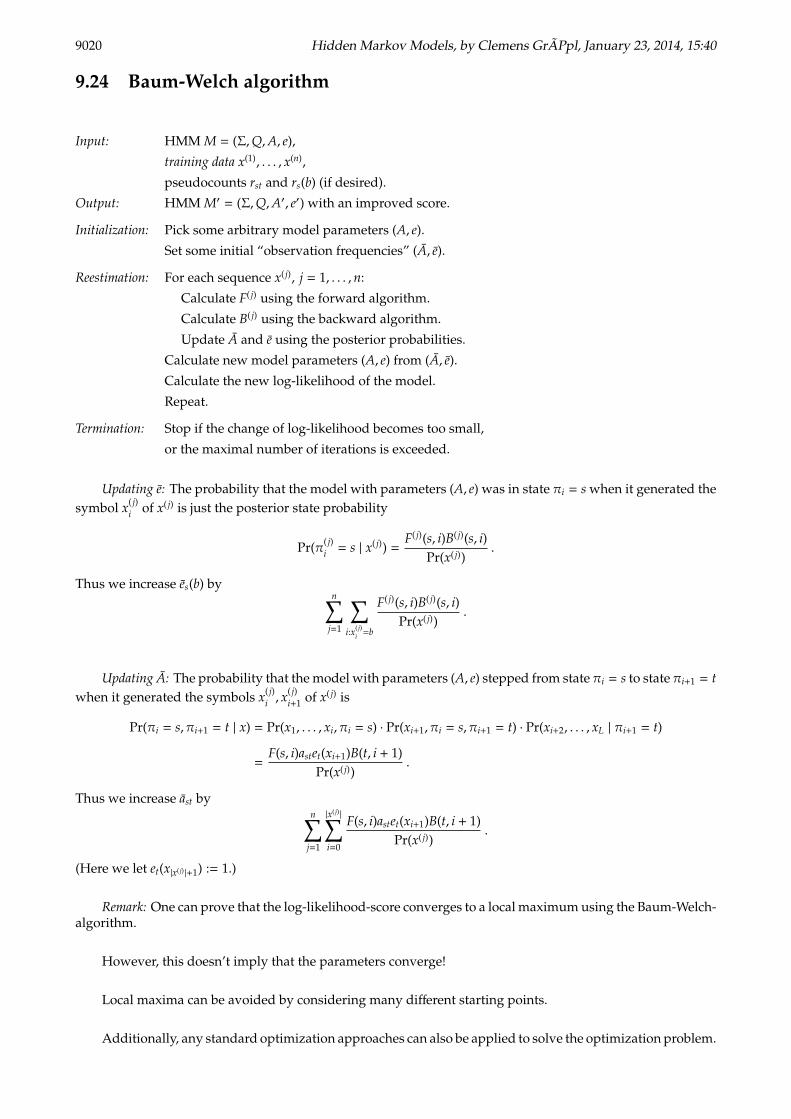
9.24 Baum-Welch algorithm

Input: HMM M = (Σ,Q,A, e),

training data x(1), . . . , x(n),

pseudocounts rst and rs(b) (if desired).

Output: HMM M′ = (Σ,Q,A′, e′) with an improved score.

Initialization: Pick some arbitrary model parameters (A, e).

Set some initial “observation frequencies” (A, e).

Reestimation: For each sequence x( j), j = 1, . . . ,n:

Calculate F( j) using the forward algorithm.

Calculate B( j) using the backward algorithm.

Update A and e using the posterior probabilities.

Calculate new model parameters (A, e) from (A, e).

Calculate the new log-likelihood of the model.

Repeat.

Termination: Stop if the change of log-likelihood becomes too small,

or the maximal number of iterations is exceeded.

Updating e: The probability that the model with parameters (A, e) was in state πi = s when it generated thesymbol x( j)

i of x( j) is just the posterior state probability

Pr(π( j)i = s | x( j)) =

F( j)(s, i)B( j)(s, i)Pr(x( j))

.

Thus we increase es(b) byn∑

j=1

∑i:x( j)

i =b

F( j)(s, i)B( j)(s, i)Pr(x( j))

.

Updating A: The probability that the model with parameters (A, e) stepped from state πi = s to state πi+1 = twhen it generated the symbols x( j)

i , x( j)i+1 of x( j) is

Pr(πi = s, πi+1 = t | x) = Pr(x1, . . . , xi, πi = s) · Pr(xi+1, πi = s, πi+1 = t) · Pr(xi+2, . . . , xL | πi+1 = t)

=F(s, i)astet(xi+1)B(t, i + 1)

Pr(x( j)).

Thus we increase ast byn∑

j=1

|x( j)|∑

i=0

F(s, i)astet(xi+1)B(t, i + 1)Pr(x( j))

.

(Here we let et(x|x( j) |+1) := 1.)

Remark: One can prove that the log-likelihood-score converges to a local maximum using the Baum-Welch-algorithm.

However, this doesn’t imply that the parameters converge!

Local maxima can be avoided by considering many different starting points.

Additionally, any standard optimization approaches can also be applied to solve the optimization problem.


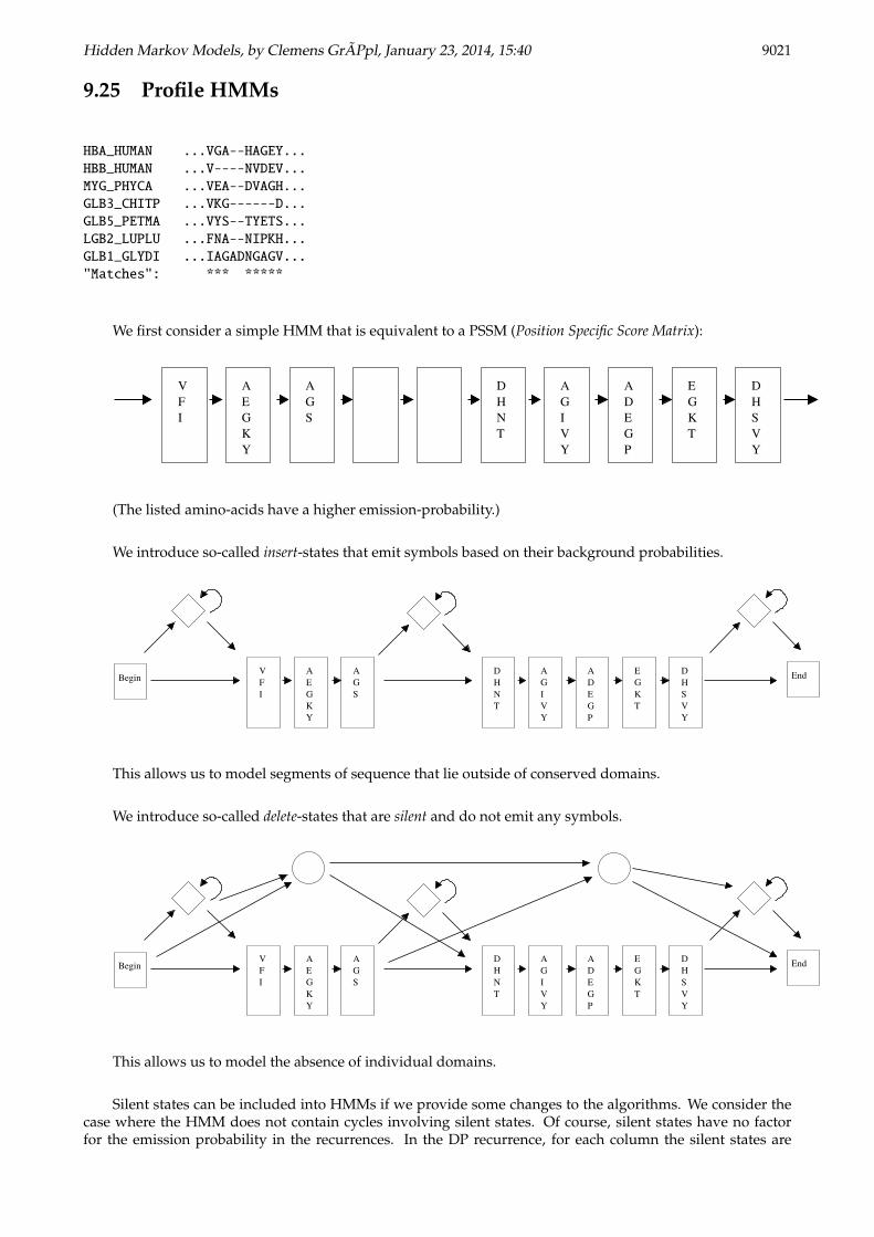
9.25 Profile HMMs

HBA_HUMAN ...VGA--HAGEY...

HBB_HUMAN ...V----NVDEV...

MYG_PHYCA ...VEA--DVAGH...

GLB3_CHITP ...VKG------D...

GLB5_PETMA ...VYS--TYETS...

LGB2_LUPLU ...FNA--NIPKH...

GLB1_GLYDI ...IAGADNGAGV...

"Matches": *** *****

We first consider a simple HMM that is equivalent to a PSSM (Position Specific Score Matrix):

ADEGP

AEGKY

VFI

AGS

DHNT

AGIVY

EGKT

HSVY

D

(The listed amino-acids have a higher emission-probability.)

We introduce so-called insert-states that emit symbols based on their background probabilities.

ADEGP

AEGKY

VFI

AGS

DHNT

AGIVY

EGKT

HSVY

DBegin End

This allows us to model segments of sequence that lie outside of conserved domains.

We introduce so-called delete-states that are silent and do not emit any symbols.

ADEGP

AEGKY

VFI

AGS

DHNT

AGIVY

EGKT

HSVY

DBegin End

This allows us to model the absence of individual domains.

Silent states can be included into HMMs if we provide some changes to the algorithms. We consider thecase where the HMM does not contain cycles involving silent states. Of course, silent states have no factorfor the emission probability in the recurrences. In the DP recurrence, for each column the silent states are


processed after the emitting states. They receive incoming paths from the same column. We do not describethe details here.

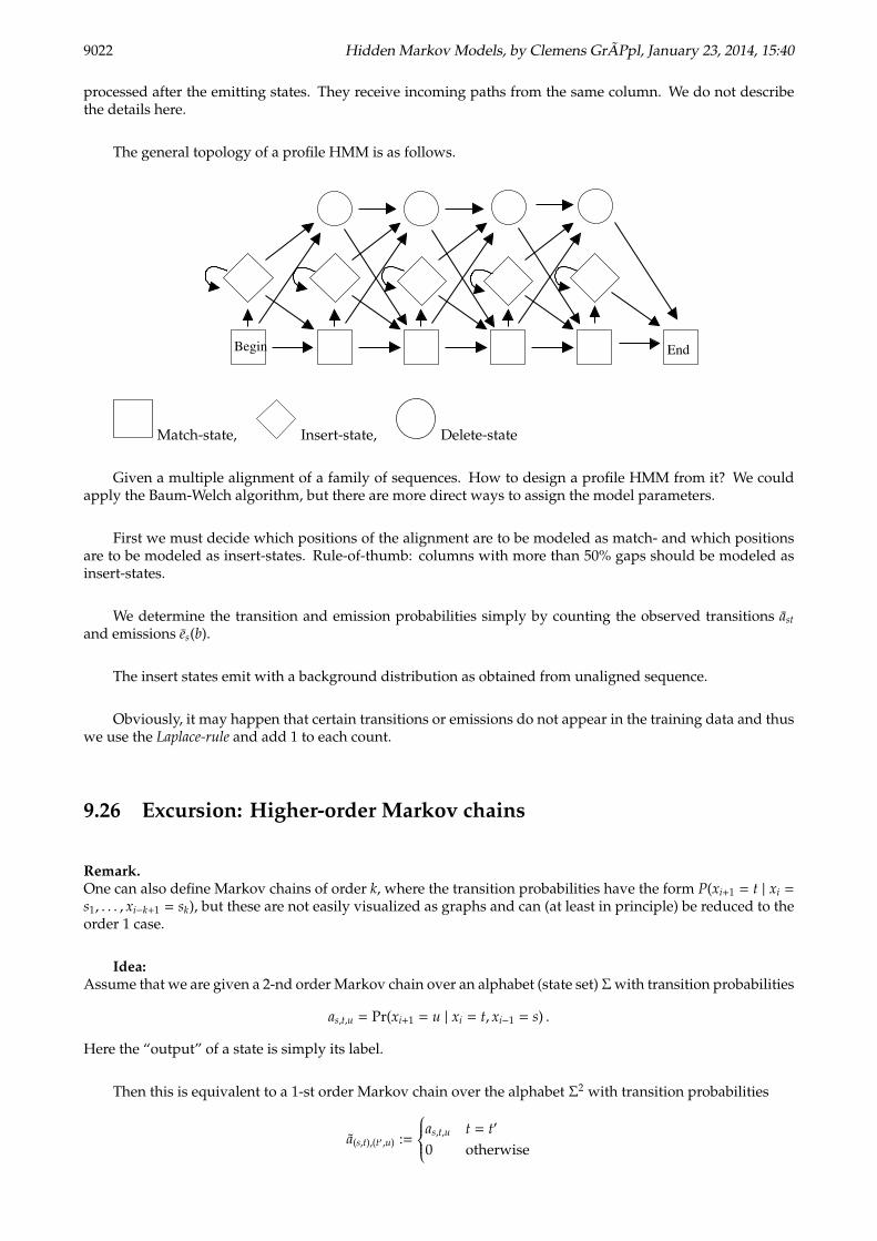
The general topology of a profile HMM is as follows.

Begin End

Match-state, Insert-state, Delete-state

Given a multiple alignment of a family of sequences. How to design a profile HMM from it? We couldapply the Baum-Welch algorithm, but there are more direct ways to assign the model parameters.

First we must decide which positions of the alignment are to be modeled as match- and which positionsare to be modeled as insert-states. Rule-of-thumb: columns with more than 50% gaps should be modeled asinsert-states.

We determine the transition and emission probabilities simply by counting the observed transitions astand emissions es(b).

The insert states emit with a background distribution as obtained from unaligned sequence.

Obviously, it may happen that certain transitions or emissions do not appear in the training data and thuswe use the Laplace-rule and add 1 to each count.

9.26 Excursion: Higher-order Markov chains

Remark.One can also define Markov chains of order k, where the transition probabilities have the form P(xi+1 = t | xi =s1, . . . , xi−k+1 = sk), but these are not easily visualized as graphs and can (at least in principle) be reduced to theorder 1 case.

Idea:Assume that we are given a 2-nd order Markov chain over an alphabet (state set) Σ with transition probabilities

as,t,u = Pr(xi+1 = u | xi = t, xi−1 = s) .

Here the “output” of a state is simply its label.

Then this is equivalent to a 1-st order Markov chain over the alphabet Σ2 with transition probabilities

a(s,t),(t′,u) :=

as,t,u t = t′

0 otherwise


The “output” of a state (t,u) is its last entry, u.

Begin and end of a sequence can be modeled using a special state 0, as before. The reduction of k-thorder Markov chains uses Σk in a similar way. (Proof: exercise.) – However, usually it is better to modify thealgorithms rather than blow up the state space.

9 markov chains and hidden markov models - freie … · 9 markov chains and hidden markov models we...

Documents