1(18) ITS 2004, Berlin, Sep 4-7, 2004

Market Analysis of Mobile Handsets Subsidies

Fawzi Daoud, Heikki Hämmäinen Networking Laboratory

Helsinki University of Technology P.O. Box 3000, FIN-02015 HUT, Finland

{daoud@netlab.hut.fi, heikki.hammainen@hut.fi) Abstract

Subsidies are a widespread practice to allow consumers to get their mobile handsets at deep discount, or even for free. Recently, with 3G and subsequent requirements on sophisticated and costly handsets, subsidies are being reconsidered both in subsidized and non-subsidized markets. In this paper, we analyse the requirements for subsidies with respect to economic efficiency. Using a simplified analytical model with linear demand and supply we illustrate the relationship of subsidies with market factors such as penetration rate, churn rate, country type (developed/developing), and charging type (prepaid/postpaid). Korea, Japan, Finland, and the UK are chosen as case markets since they represent different strategies for handsets subsidies. Our main conclusion is that consumer subsidies, either government- or operator-funded, can be economically efficient from the national viewpoint when applied for faster adoption of a specific technology at the right time window in a temporary manner. Keywords Mobile handsets, mobile markets, elasticity, penetration

1 Definition of subsidies

There is no widely accepted definition of what constitutes a subsidy. However, according to the World Trade Organisation (WTO), a subsidy contains three elements: (i) a financial contribution (ii) by a government or any public body within the territory of a member (iii) which confers a benefit. Generally on the international level subsidies are thought of as cash payments from a government to a producer or consumer, but subsidies may appear in many formats (see Table 1). Some have a direct effect on price, like grants and tax exemptions, while others act indirectly, for example, through regulations that bias the market in favor of a government-sponsored technology.

Form of Intervention Example

1. Direct Financial Transfer Grants to producer or consumers, low interest loans 2. Regulation of a sector Demand guarantees, price controls, market access

restrictions 3. Trade restrictions Quotas, trade embargoes, technical restrictions 4. Preferential tax treatment Rebates, exemptions on royalties, tax credit,

accelerated depreciation

Table 1. Types of Subsidies

2(18) ITS 2004, Berlin, Sep 4-7, 2004

The exact consequence of any government subsidy is dependent on the specific national circumstances to which it is applied. As the context and characteristics of the market system vary, so do the barriers and potential ways of overcoming these. Forms of possible market distortions include: • Subsidies reducing consumer prices may cut incentives to use products more efficiently; • Subsidies reducing producer costs may cut incentives to minimize costs, resulting in less efficient operation and investments; • By reducing the revenue received by producers, subsidies can undermine their ability and incentive to invest in new infrastructure; • Direct subsidies in the form of grants or tax exemptions act as a drain on government finances; • Price caps or ceilings below market-clearing levels may lead to physical shortages and a need for administratively costly rationing arrangements; • By increasing sales, consumption subsidies may increase import or decrease the amount available for export; and • Subsidies to a specific technology can undermine the development and commercialisation of other promising technologies. We are interested in handset subsidies granted by a government or operator and appearing to consumers as lower handset prices.

2 Case Markets

The market phase and government policy of our case markets are briefly summarized as follows. In Japan, cellular phone service was first introduced in 1979. In 1994, customer ownership of handsets was introduced, and subsidies for handsets have been general practice. In 1999, successful iMode service was launched. The number of subscribers of 2nd generation PDC mobile phones exceeded that of fixed phones late 2000. 3G licenses have been granted in 2000 to three carrier groups based on beauty contest. 3G services were introduced in 2001. Deregulation accelerated the growth of mobile services in the 1990s. In Korea, cellular phone service was first introduced in 1984. In 2000, the number of CDMA subscribers exceeded that of fixed telephony. 3G licenses were granted in 2001 to three carrier groups based on auction, totaling in the amount of 2.9 billion $. Korea was the first country to introduce CDMA2000-1X in 2000. The fast growth of penetration was partially due to the introduction of competition in the market in 1996, and due to handset subsidies coordinated by the regulator. Finland was the first country to introduce the digital GSM standard in 1992. The country has long been the leader in mobile penetration, although itit was essentially a duopoly until 1998. Mobile revenue surpassed fixed line revenue in 1997. Finland has been the first country to grant 3G licenses in 1999 to four carrier groups based on beauty contest. Regulator has not allowed direct handset subsidies in Finland. In the UK, cellular service was started in 1984 with two operators. GSM was introduced in 1993. The UK has been a very competitive market, with more operators than other European countries. 3G licenses were granted in 2000 to five carrier groups based on auction, totaling the amount of 35 Billion $. Handset subsidies exist in the UK.

3(18) ITS 2004, Berlin, Sep 4-7, 2004

3 Rationale for handset subsidies

Handset subsidies may emerge for various reasons, but we focus on drivers having potential strategic relevance to governments and regulators.

3.1 Critical Mass for a New Technology

Handset subsidy could help getting a critical mass for a new technology. In Japan subsidies are a common practice and the market has been able to adopt new technologies rapidly: 70 million subscribers for i-mode and 14 million for CDMA2000 in a relatively short time. In Korea, the deployment of CDMA was slow until 1996 when handset subsidies were introduced. In year 2000 handset subsidies were banned in Korea when the growth rate of penetration slowed down. In April 2004, Korea again allowed subsidies for WCDMA to achieve the critical mass. In comparison, European countries have been slow in deploying WCDMA. While market data about WCDMA deployment is still immature, cases of Korea and Japan show that handset subsidies could be a strategic tool for speeding up the market.

3.2 New Business Model for New Services

Most European markets are handset-centric in a sense that the handset and the mobile service are only loosely bundled. Japan and Korea are more service-centric as consumers buy the service and handset together, and the operator has a stronger role as a handset channel. So far at least in Japan the service-centric model has been successful in introducing new data services. It has enabled the operator-driven end-to-end orchestration of new services and business models. Large mobile operators like NTT DoCoMo are closely cooperating with handset vendors to deploy new services based on specific handset capabilities. In addition, Vodafone is gaining experience from the Japanese market and aims to implement similar models for instance in the UK. Handset subsidies move control and responsibilities from handset vendors to operators can thus be considered as a key part of the service-centric orchestration strategy.

Figure 1. Economic analysis of the subsidy

P*

P**

Q Q*

P**-S

Subsidy

1.1.1

Quantity Subscriptions

DD

S

A B

C F

E

4(18) ITS 2004, Berlin, Sep 4-7, 2004

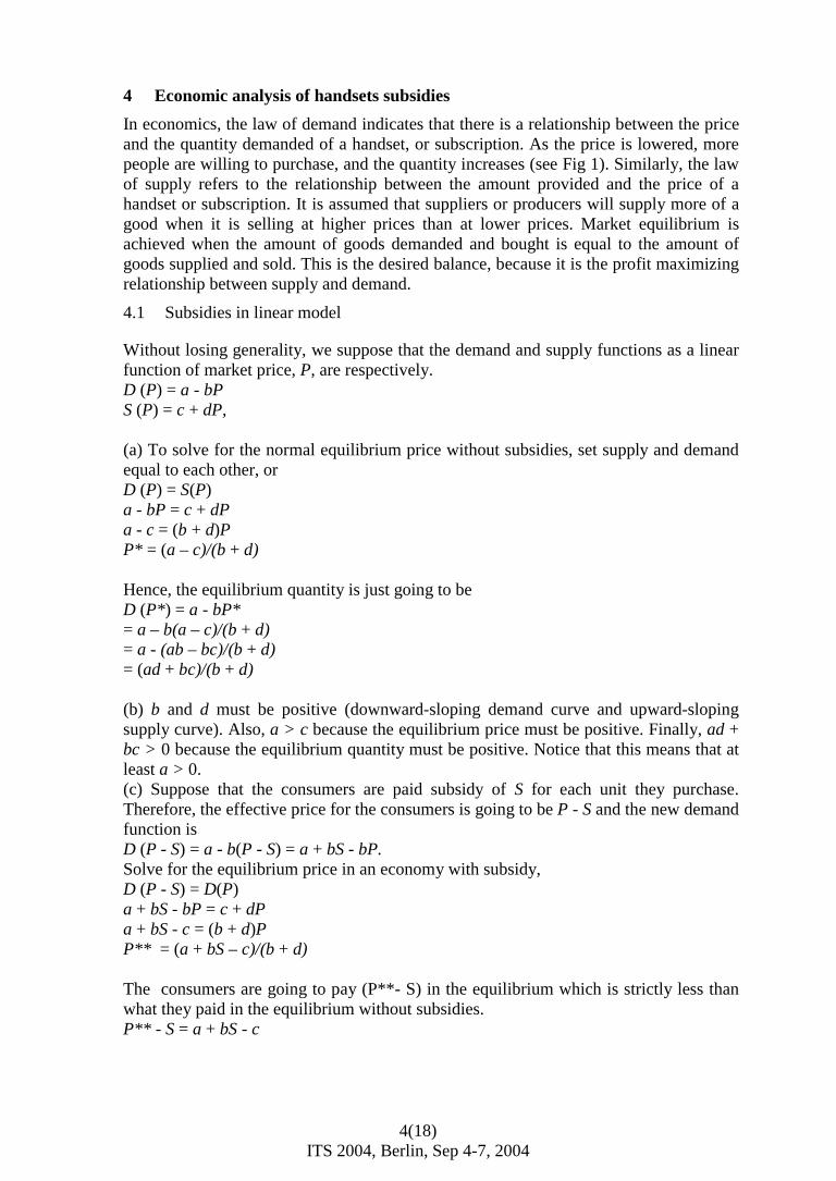
4 Economic analysis of handsets subsidies

In economics, the law of demand indicates that there is a relationship between the price and the quantity demanded of a handset, or subscription. As the price is lowered, more people are willing to purchase, and the quantity increases (see Fig 1). Similarly, the law of supply refers to the relationship between the amount provided and the price of a handset or subscription. It is assumed that suppliers or producers will supply more of a good when it is selling at higher prices than at lower prices. Market equilibrium is achieved when the amount of goods demanded and bought is equal to the amount of goods supplied and sold. This is the desired balance, because it is the profit maximizing relationship between supply and demand.

4.1 Subsidies in linear model

Without losing generality, we suppose that the demand and supply functions as a linear function of market price, P, are respectively. D (P) = a - bP S (P) = c + dP, (a) To solve for the normal equilibrium price without subsidies, set supply and demand equal to each other, or D (P) = S(P) a - bP = c + dP a - c = (b + d)P P* = (a – c)/(b + d) Hence, the equilibrium quantity is just going to be D (P*) = a - bP* = a – b(a – c)/(b + d) = a - (ab – bc)/(b + d) = (ad + bc)/(b + d) (b) b and d must be positive (downward-sloping demand curve and upward-sloping supply curve). Also, a > c because the equilibrium price must be positive. Finally, ad + bc > 0 because the equilibrium quantity must be positive. Notice that this means that at least a > 0. (c) Suppose that the consumers are paid subsidy of S for each unit they purchase. Therefore, the effective price for the consumers is going to be P - S and the new demand function is D (P - S) = a - b(P - S) = a + bS - bP. Solve for the equilibrium price in an economy with subsidy, D (P - S) = D(P) a + bS - bP = c + dP a + bS - c = (b + d)P P** = (a + bS – c)/(b + d) The consumers are going to pay (P**- S) in the equilibrium which is strictly less than what they paid in the equilibrium without subsidies. P** - S = a + bS - c

5(18) ITS 2004, Berlin, Sep 4-7, 2004

= (a + bS - c - bS – dS)/(b + d) = (a - c – dS)/(b + d) = P* -dS/(b + d) < P* Finally, the equilibrium quantity with subsidies is going to be D (P** - S) = a - b(P** - S) = a - b(a - c – dS)/(b + d) = a –(ab - bc – bdS)/(b + d) = (ab + ad - ab + bc + bdS)/(b + d) = ad + bc + bdS/(b + d) Q** = ad + bc + bdS/(b + d) = Q* + bdS/(b + d) > Q*, Q** is strictly more than in the equilibrium without subsidies Q*. (d) To summarize, with subsidies the consumers are paying P** - S = (a - c – dS)/(b + d), the quantity traded is going to be Q** = (ad + bc + bdS)/(b + d) The net increase in consumer surplus is ∆CS= C+F in the figure ∆CS = 0.5 * (P* - P**) * [D(P*) + D(P**)] = 0.5 * [(dS)/(b + d)]*[(2ad+2bc+bdS)/(b + d)] = [0.5*dS* (2bc + 2ad + bdS)]/(b + d)2 Depending on who is funding the subsidy, the surplus and loss may be distributed differently. We consider mainly two different cases.

4.2 State subsidy

The state can fully pay the subsidy, or one part of it. In this case the total cost of the state subsidy is TC = S * (Q**) = adS + bcS + bdS2/(b + d). One part of it goes to the consumer with the same amount computer above. The other part goes to the supplier that would receive a price P** = (a + bS – c)/(b + d) = P* + bS/(b + d) > P* in the equilibrium which is strictly more than what they obtained in the equilibrium without subsidies.

4.3 Mobile operator subsidy

The operator can pay the subsidy either from independent sources or from the revenues generated by other profitable services. The cost of the subsidy that the operator should fund is TC = [(P* - P** + S) * Q**] + [ (P**- P*) * (Q**- Q*)/2] = [dS/(b + d) * (ad + bc + bdS)/(b + d)] + [bS/ 2(b+d) * bdS/(b + d) ] = [dS/ (b+d)2 ] * [ad+bc+bdS +b2S/2] We notice here that we added the part [ (P**- P*) * (Q**- Q*)/2], because normally this would be part of the deadweight loss that the operator should also fund as it is taking all the risks. If the operator is cross-subsidizing handsets using other sources of revenues, a condition for not having a loss is that marginal revenues of these others services are higher than the costs for the handset subsidies. Generally, mobile operators use other revenue sources from roaming services and call termination services, added to the subscriptions. Then we may have MR(roaming) + MR (call termination) + MR (subscriptions+usage) >= TC

6(18) ITS 2004, Berlin, Sep 4-7, 2004

The marginal revenues from subscriptions may be low at the beginning. Take the case of a network with about 1 million customers.Let’s assume their operating cost is 200 million euros a year. If their ARPU is 30 euros per month, the operating cost relating to subsidies would have already consumed nearly 7 months worth of revenue. If operators assume that only at the end of 2-years contract, they would refund the subsidy investment, this involves much high risks. On the other hand, the gain generated by the increase of demand on the supplier side is ∆G = A+B in the figure ∆G = 0.5 * (P** - P*) * [S(P**) + S(P*)] = 0.5 *[(bS)*(2ad + 2bc + bdS)]/(b + d)2 The total cost of the subsidy is ∆C = S * (Q** - Q*) = S*(ad+bc+dbS)/b+d) = A+B+C+E+F in the figure So the real surplus/loss of the supplier (network operator) is ∆SS= -C-E-F in the figure ∆SS= ∆G - ∆C = [0.5 *[(bS)*(2ad + 2bc + bdS)]/(b + d)2 ] - [S*(b+d)*(ad+bc+dbS)/(b+d)2] We could calculate the deadweight loss, ∆W = E in the figure ∆W = ∆CS + ∆SS = - 0.5* dbS2/(d+b) As we see here, giving a fixed subsidy amount per product/handset generates a deadweight loss. The mobile operator, in case of cross-subsidizing, should also cover the amount of the deadweight loss. To reduce the amount of deadweight loss, we could think of substituting fixed subsidy by a subsidy with a changing amount. We would consider this case later in this paper when addressing removal of subsidies.

5 Elasticity effects of subsidies

Conceptually, elasticity is a measure of responsiveness. The effects of the subsidy on the equilibrium quantity and price depend on the elasticity of supply and demand. Algebraically, it is the ratio of two percentage changes. We distinguish elasticity of demand εd and elasticity of supply εs. There’s an important relationship between subsidies and elasticity. Buyer benefits of subsidy if εd/εs is small. Sellers benefits of subsidy if εd/εs is big. The more inelastic the demand is, the lower percentage of these subsidies the consumers receive, given the supply elasticity. The more inelastic the supply is, the lower percentage sellers benefit, given the demand elasticity. As elasticity changes with demand increase, subsidies are more efficient during the time window where elasticity is positive.

Figure 2. Generic Product Life Cycle

7(18) ITS 2004, Berlin, Sep 4-7, 2004

There is numerous empirical evidence that shows that demand for some products grows over time until the market reaches its maturity, and gradually decays thereafter. The so-called theory of the product life cycle (PLC) provides a foundation to this pattern of consumer behavior based on diffusion models. This pattern of inter-temporal changes in demand has certainly become a stylized fact for certain products such as durable goods. The standard product life cycle tends to have five or six phases: development, introduction, growth, maturity, and decline. It can be shown graphically with two lines - one to show the level of profit, and one to show the level of sales. Firms will often try to use extension strategies. These are techniques to try to delay the decline stage of the product life cycle. The maturity stage is a good stage for the company in terms of generating cash. The costs of developing the product and establishing it in the market are paid and it tends to then be at a profitable stage. The longer the company can extend this stage the better it will be for them.

Figure 3. Penetration and penetration growth in the 4 countries (Korea is a specific case)

Current graphs for wireless 2G penetration in most developed countries have reached points where the percentage of penetration increase is becoming lower over time. In our

8(18) ITS 2004, Berlin, Sep 4-7, 2004

case, Japan and Finland have reached this point at an early stage, even that it relates to different penetration rates. Generally, these points took place within 1998-2000. This shows that the market has reached the maturity phase. Elasticity has been then decreasing gradually. When approaching the saturation point, incentives based on price subsidies may become non-effective, because the number of subscribers could not be increased much more. The analysis of the % penetration increase in different continents, as indicated in the figure, shows that there’s generally some slow down. In Western Europe, the growth has reached its maximum during 1999. For North America, this increase has been low but more stable. In South America, the increase has slowed down in 1998, and then increased shortly within 1999, before decreasing again. Some parts of the world, that are not represented in the figure may still have some increase at a low rate.The markets of the developing world, for instance, are unlikely to support the high levels of subscriber penetration seen in Europe. So there should be a level of ultimate penetration a region can support, and the time frame on which we get there. We could assume that when penetration reaches ‘growth saturation’ depending on countries (about 63% within Europe), the rate of proportional growth begins to decline from the consistent historical level of about 1.6x. When the ‘overall saturation’ level is reached, penetration comes close to zero growth (a proportional growth of 1.0 times or just over).

Figure 4. Global penetration growth From the figure on Korean 2G wireless penetration, it is noticeable that before 1997, penetration was low for 2G. The regulator allowed subsidies until 2000. That had a tremendous effect on penetration growth. For WCDMA, the Korean regulator seems to act similarly, by giving subsidies, to increase penetration of this technology.

6 Elasticity of Demand

ELASTICITY DEMAND = (∆% Q)/(∆%P)= dQ/dP.(P/Q) Percentage change in quantity demanded due to an increase in price divided by percentage change in price. εd = -b*P/Q =-P/(a/b-P).

9(18) ITS 2004, Berlin, Sep 4-7, 2004

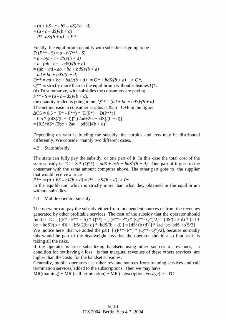
It is always negative due to the Law of Demand. At points with a high price and low quantity, demand is elastic. At points with a low price and high quantity, demand is inelastic. It depends on several factors: availability of close substitutes proportion of the consumer’s budget spent on that good time horizon

Figure 5. Kinds of demand elasticity

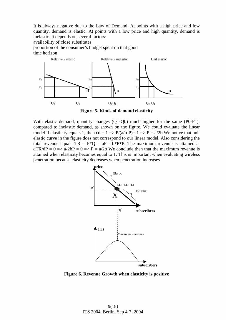
With elastic demand, quantity changes (Q1-Q0) much higher for the same (P0-P1), compared to inelastic demand, as shown on the figure. We could evaluate the linear model if elasticity equals 1, then εd = 1 => P/(a/b-P)= 1 => P = a/2b.We notice that unit elastic curve in the figure does not correspond to our linear model. Also considering the total revenue equals TR = P*Q = aP - b*P*P. The maximum revenue is attained at dTR/dP = 0 => a-2bP = 0 => P = a/2b We conclude then that the maximum revenue is attained when elasticity becomes equal to 1. This is important when evaluating wireless penetration because elasticity decreases when penetration increases

Figure 6. Revenue Growth when elasticity is positive

price

1.1.1.1.1.1.1.1

Elastic

q’

p’

subscribers

Inelastic

X

1.1.1

Maximum Revenues

subscribers

10(18) ITS 2004, Berlin, Sep 4-7, 2004

As the marginal revenue MR equals dTR/dP = a – 2 bP. In the elastic region of the demand, marginal revenue is positive. In the inelastic region of the demand, marginal revenue is negative. Also, we interpret this as we need to reduce the part where marginal revenue is negative. So the cost of the subsidy should be reduced as much as demand becomes inelastic.

7 Elasticity of Supply

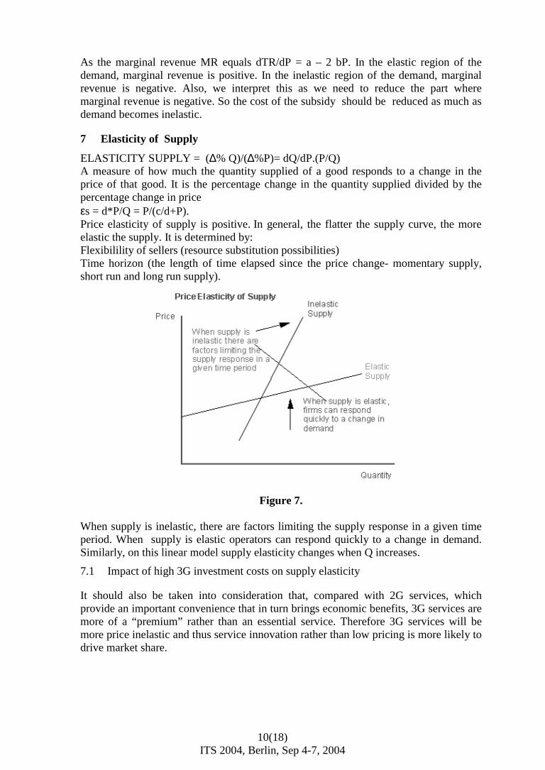
ELASTICITY SUPPLY = (∆% Q)/(∆%P)= dQ/dP.(P/Q) A measure of how much the quantity supplied of a good responds to a change in the price of that good. It is the percentage change in the quantity supplied divided by the percentage change in price εs = d*P/Q = P/(c/d+P). Price elasticity of supply is positive. In general, the flatter the supply curve, the more elastic the supply. It is determined by: Flexibilility of sellers (resource substitution possibilities) Time horizon (the length of time elapsed since the price change- momentary supply, short run and long run supply).

Figure 7.

When supply is inelastic, there are factors limiting the supply response in a given time period. When supply is elastic operators can respond quickly to a change in demand. Similarly, on this linear model supply elasticity changes when Q increases.

7.1 Impact of high 3G investment costs on supply elasticity

It should also be taken into consideration that, compared with 2G services, which provide an important convenience that in turn brings economic benefits, 3G services are more of a “premium” rather than an essential service. Therefore 3G services will be more price inelastic and thus service innovation rather than low pricing is more likely to drive market share.

11(18) ITS 2004, Berlin, Sep 4-7, 2004

Japan and Korea have been leaders in supplying 3G networks. While CDMA2000-1X networks that are intermediate 3G have been successful in attracting subscribers, WCDMA 3G technology has been facing problems for rollout due to high costs etc. The numerous 3G licenses and coverage requirements translate into significant investments in 3G networks. At the same time, because of the downturn in the telecom sector, the severe CAPEX reduction programs that operators are confronted with nowadays lowered their level of equipment purchases in wireless networks. The expectation in their future performance as reflected in their stock prices have decreased, and the debt position of mobile operators has increased, which has weakened their negotiation power with financial markets to raise funding. These cost reductions, which have been worsened by the outcome of 3G licensing (e.g., high license fees), can already be felt for the 3G market, as operators are delaying the rollout of 3G networks, sharing part of the rollout costs with other players or even pulling out from markets less attractive to them. As a consequence, many equipment vendors are finding themselves in a difficult financial situation. The mobile telecom industry has increasingly put pressure on national regulators to relax certain specific 3G license conditions, in particular those that have an explicit impact on the short-term funding problems of a number of mobile operators, both 2G and 3G. These regulatory revisions currently focus on delays of coverage obligations, reduction of and/ or delays in license fee payments, extension of license durations and infrastructure sharing considerations. All these measures result in a relaxation of the pressure on the debt of the operators and a decrease of short- term financing requirements. The extension of the license duration allows for a longer payback period and years of profitability.

Figure 8.

8 Service Bundling improves elasticity

The strategies of market segmentation by Japanese and Korean telecom operators have been very different from those of Europe. In Europe, operators focus on branding their company name in general like Vodafone etc, but they have been criticized for poor understanding of what the users really want. The services that have been launched have not been well received in the market. The regulators at national and regional level may have an important role to play at this level. In Korea and Japan, regulators have been active to allow development of mass markets of mobile internet and they let the large mobile operators (e.g NTT) control the business model. In Europe in general, regulators have been more passive in this sense,

12(18) ITS 2004, Berlin, Sep 4-7, 2004

probably because the markets were developing well for 2G. For 3G, the situation is different, as for example Finland and UK are delaying the mass market deployment, because of financial risks etc. The European regulators may have a new role to play to fix this. Integrating and bundling services improves the responsiveness of mobile operators to new markets. This improves the supply elasticity for new technologies. Docomo in Japan has been leader in this area with i-mode services, as it acts as a service integrator. While in Japan all four handset manufacturers are given handset specifications by DoCoMo, the European manufacturers specify the phone attributes (for example, user interface, internal storage size) themselves. Specifications are therefore in the hands of the numerous implementers, making it much harder for content to be compatible on all handsets. One key observation is that i-mode was, from the start, a complete and fully functioning service/product concept. The i-mode service is still growing, and now it is focusing on how to connect with real-world needs. “Put everything you carry around into your mobile”. Docomo acts as mobile portal where different services are integrated with i-mode. It has the full responsibility about adding new value added services to the core i-mode. Docomo receives the revenues, and then distributes a percentage to the service providers This full control of the value chain ensures a high quality of service, and helps discovery and elimination of Spam. I-mode is practically based on location-based service (i-area), where different other services are integrated to service specific segments. Depending on the location of the user, different information is provided about hotels, restaurants, events, entertainment etc. Then associated services could be launched dynamically. For example, Cmode™ service allows subscribers to buy beverages or information content by communicating with vending machines using their mobile phones. By charging prepaid money onto their phones, subscribers no longer need to search for small change when buying soft drinks from vending machines. They can make a purchase just by holding up their phones and pressing a button. Similarly in Korea, location information service and mobile banking have attained high level of usage for different segments. Creating customer databases based on this information helps the Korean operators identify exactly what kind of services their customers are looking for, and enables them to offer these at premium prices. Teenagers are clearly the group that is driving the market, spending around three times more per user on mobile data services. Korean operators effectively use completely different brand names for different market segments. They have managed to segment the market efficiently and emphasized the importance of customer relationship management. Creating customer databases based on this information helps the Korean operators identify exactly what kind of services their customers are looking for, and enables them to offer these at premium prices. The segmentation is based on age groups, and content provided to each group differs a lot. Services beyond only wireless are provided: Internet Portals, dedicated Internet cafes for customers, and a number of discounts on restaurants, cinemas etc. Direct marketing and advertising is used to target these groups. Examples include discount coupons for department stores and prescreening of movies. Examples some of SKTelecom’s products are June, TTL ting and UTO. TTL Ting targets a teenage group from 13 to 18 whereas UTO is aimed at adults, aged from 25-35 with a high disposable income. These products are designed to provide customized services to match the life-style of individual customers. By focusing on narrow segments based on membership, Korean

13(18) ITS 2004, Berlin, Sep 4-7, 2004

operators can gather detailed customer information that can be very valuable to the operators. Gaming is vastly popular in Japan (40 millions) and Korea (10 millions). In contrast to many European and Asia-Pacific counterparts, Japanese and Korean operators adopted a mass-market strategy to promote mobile gaming at early stages of market development. Operators focused on selected content including gaming, entertainment and ring tones and made it widely available. Mobile gaming was not singled out as a premium service. The spin-off of this strategy was that operators could also understand the demand for mobile services better and segment their customer bases more effectively.

Figure 9. Similarly in large markets emphasis placed on bundled services by carriers is beginning to pay off, with a growing number of consumers purchasing fixed, Internet access, cable and satellite TV, and wireless as part of a multi-service bundle. Bundles offer numerous benefits to the consumer, including discounted pricing, the convenience of a single bill, and a single point of contact for customer service. They also yield significant dividends for carriers in the form of reduced subscriber churn, increased average revenue per user (ARPU), and lower operational support costs. Profiling and analysis of wireless subscribers currently purchasing a telecom bundle found that they are most likely to be members of demographic segments that are highly attractive to carriers: ages 30-49, residents of suburban areas, and well-educated, with high household income. Another subscription model, the prepaid services, may also allow mobile operators to penetrate new segments of their market (teenagers, occasional users, transient travelers,..) and to differentiate their tariffs and product portfolios. In essence, the barrier to mass-market adoption of the mobile phone was the high start up cost of a fixed-term contract account. Since this hurdle to adoption was removed with the advent of prepaid phones, market saturation has effectively taken place in some countries with higher than 80-90% and will likely follow in many others. It has also allowed virtual mobile operators to launch products easily and to provide low-cost options for the broadest (and quickest) market penetration.

14(18) ITS 2004, Berlin, Sep 4-7, 2004

9 Cross elasticity of demand

Cross-elasticity: ε XY = (∆%Q X)/( ∆%P Y) It is a measure of how much the quantity demanded of one good responds to a change in the price of another good. It is computed as the percentage change in the quantity demanded of the first good divided by the percentage change in the price of the second good. This is related to churn rates between products. Substitutes have positive cross price elasticities. Complements have negative cross price elasticities ε XY > 1 = The products are closely related. A change in Y will greatly change X. ε XY < 1 = The products are loosely related. A change in Y will loosely change X. ε XY = 0 = The products have no relationship. In a perfectly homogenous goods industry without switching costs, consumers are indifferent between the goods offered by competing firms. Consequently, a slight increase in the price of one of the firms would lead to a large decrease in the volume of its sales – that is, the cross-elasticity of demand would be high. However, in an industry with switching costs, a firm with a large base of locked-in consumers can raise its price without losing significant business to competitors and so the expected cross-elasticity would be low. A low firm level cross-elasticity can consequently indicate the presence of switching costs.

10 Churn elasticity

The churn phenomenon appears when customers switch from one operator to another or who abandon cellular services entirely. With more competitors and new service offerings, elasticity increases and carriers have to work harder to win the loyalty of profitable customers. Wireless Internet connectivity is introducing a whole new range of choices and level of complexity for mobile phone users who already find it hard to discern the benefits of new technology and advantages of different service plans. Also, as mobile service becomes commoditized, customers are finding the barriers to switching low and are easily enticed away, even for the smallest of reasons.

Figure 10. Churn Reasons Recent analysis of data clients suggests price-related factors are major causes of voluntary churn. New customers may churn because they were sold a plan that didn’t match their calling needs, but they couldn’t find an appropriate plan, or they tried and

15(18) ITS 2004, Berlin, Sep 4-7, 2004

couldn’t switch. Many customers also voluntarily leave their carrier because they don’t fully understand its rate plans, which include various mixes of call charges, free minutes, service features, handset offers, etc. It’s easy to see why customers are confused, and why they’re inclined to switch to a competitor offering a lower rate because they believe the other plan is “cheaper.”. Customers consider important factors such as coverage, transmission quality, after-sales service, product features, or the total cost of factoring in “free minutes” and other benefits. Customers who are unaware or uncertain about new products and service offerings frequently choose to abandon a carrier that has not been proactive in educating them. When evaluating churn rates in the different countries, we could say generally that more regulated countries have less churn rates than others. Churn generally varies from 1% to 40%. It depends also how we compute it (if we separate different market segments, or if we consider annual average changes, of monthly changes) . Japan has the lowest churn rate, with also Korea at low level, then we find Finland and finally UK. Also, we notice that mobile operators having higher market share have lower churn than other operators. Generally subsidies may be an incentive to keep churn rate low, assuming that there are important switching costs. We could explain that Japan and Korea have higher switching costs.

11 Subsidies Removal

Subsidies have a cost that has to be paid by the state or the mobile operator. Experience from Korea shows that allowing handset subsidies for a limited time window (e.g. 1997-2000 for 2G) seems to be effective as penetration rate grows toward saturation level. The question is then how to remove the subsidy: either removing the fixed amount of the subsidy completely at the end of the time window, or gradually removing it with a certain rate as penetration rate augments. Here we try to address these solutions and compare them.

11.1 Fixed amount subsidies removal

Suppose that after subsidies have been in the market for some time, the regulator or the operator decides to remove the fixed amount subsidy. In this case, buyers have to pay fixed amount T = S more for each subscription they purchase, compared to the equilibrium with subsidies Therefore the effective price for the buyers is going to be P+T and the new demand function is D (P+T) = a-b(P+T) The equilibrium price is going to be

Figure 11: fixed and rate based subsidy removal

Quantity Subscriptions

P*

Q*

subsidy

1.1.2

D1

S

F

D2

Rate based removal

Fixed removal

16(18) ITS 2004, Berlin, Sep 4-7, 2004

D (P+T) = S (P) a-bT –bP= c+dP P** = (a-bT-c)/ b+d The buyers are going to pay P** + T in the equilibrium that is strictly more than in the equilibrium with subsidy. P** + T = [(a-bT-c)/b+d] + T = P* + dT/b+d > P* The equilibrium quantity is going to be Q** that is strictly less than in the equilibrium with subsidy. D (P** + T) = a- b(P** + T) = (ad+bc – bdT) /b+d Q** = (ad+bc – bdT)/b+d = Q* - bdT/b+d < Q*

11.2 Rate based removal of subsidy depending on penetration

Consider now that we’d like to remove subsidy not as a fixed amount, but gradually. The consumers are going to pay proportional higher price on each product depending on usage/quantity or the penetration. This is based on a certain rate of the amount of Q. When penetration (or Q) is still low the amount to be paid is low. When Q increases, the amount to be paid is higher until all the subsidy amount is paid back. Practically, this requires that Q is known each time to compute the amount to be paid back from the subsidy. Computing exactly Q is difficult. This problem could be resolved practically by considering caps of quantity/penetration. For example when penetration changes from x% to (x+5)%, the amount to be paid back increases, say by 5%. This process could continue until all subsidy is removed. This has a positive effect on the market by reducing the deadweight loss. In this case the new demand function is Dr (P) = D(P)/1+R = a – bP / (1 + R) The equilibrium price in an economy with tax rate is going to be Dr (P) = S (P) a – bP/ 1+R = c + dP P** = (a-c-cR)/ [b + d + cR] The price P** is strictly less than what they obtained with equilibrium with subsidy as b, d, c and R are positive. The buyers are going to pay P** / (1+R) in the equilibrium P**/(1+ R) = (a-c-cR) (1+R) /(b+d + cR) The equilibrium quantity is going to be Q** that conditionally may be less than in the equilibrium with subsidy Q**= Dr (P* * ) = (a- bP**) /(1+ R)) Instead of thinking about removing an existing subsidy that is already widespread used in the market, using that rate based model. We could consider new technologies where the market is not existent yet. In this case, instead of adopting a normal fixed subsidy and then try to remove it by rate based model, we could consider more specific pricing model that considers rate based price increments as the quantity sold (or the penetration increases). In this case the new demand function is

17(18) ITS 2004, Berlin, Sep 4-7, 2004

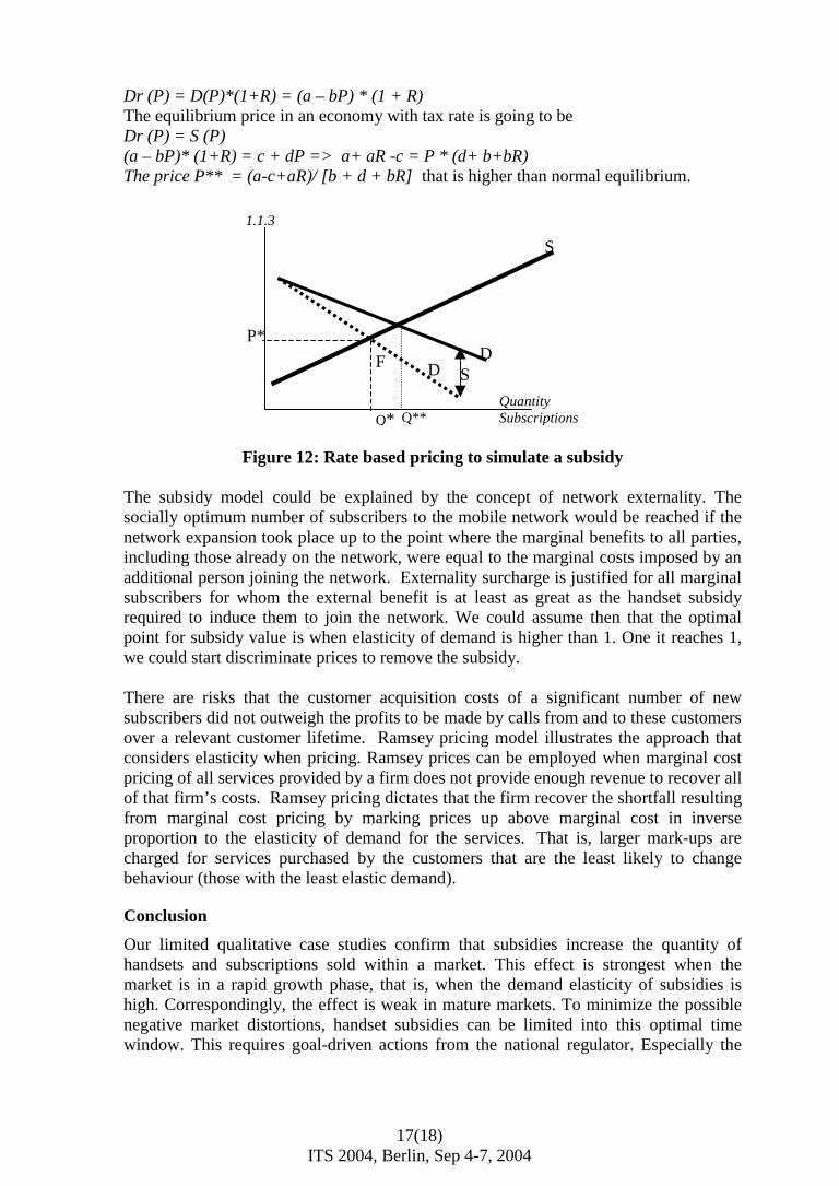
Dr (P) = D(P)*(1+R) = (a – bP) * (1 + R) The equilibrium price in an economy with tax rate is going to be Dr (P) = S (P) (a – bP)* (1+R) = c + dP => a+ aR -c = P * (d+ b+bR) The price P** = (a-c+aR)/ [b + d + bR] that is higher than normal equilibrium.

Figure 12: Rate based pricing to simulate a subsidy The subsidy model could be explained by the concept of network externality. The socially optimum number of subscribers to the mobile network would be reached if the network expansion took place up to the point where the marginal benefits to all parties, including those already on the network, were equal to the marginal costs imposed by an additional person joining the network. Externality surcharge is justified for all marginal subscribers for whom the external benefit is at least as great as the handset subsidy required to induce them to join the network. We could assume then that the optimal point for subsidy value is when elasticity of demand is higher than 1. One it reaches 1, we could start discriminate prices to remove the subsidy. There are risks that the customer acquisition costs of a significant number of new subscribers did not outweigh the profits to be made by calls from and to these customers over a relevant customer lifetime. Ramsey pricing model illustrates the approach that considers elasticity when pricing. Ramsey prices can be employed when marginal cost pricing of all services provided by a firm does not provide enough revenue to recover all of that firm’s costs. Ramsey pricing dictates that the firm recover the shortfall resulting from marginal cost pricing by marking prices up above marginal cost in inverse proportion to the elasticity of demand for the services. That is, larger mark-ups are charged for services purchased by the customers that are the least likely to change behaviour (those with the least elastic demand).

Conclusion

Our limited qualitative case studies confirm that subsidies increase the quantity of handsets and subscriptions sold within a market. This effect is strongest when the market is in a rapid growth phase, that is, when the demand elasticity of subsidies is high. Correspondingly, the effect is weak in mature markets. To minimize the possible negative market distortions, handset subsidies can be limited into this optimal time window. This requires goal-driven actions from the national regulator. Especially the

Quantity Subscriptions

P*

Q* Q**

S

1.1.3

DD

S

F

18(18) ITS 2004, Berlin, Sep 4-7, 2004

smooth termination of subsidies is a challenge because the consumer’s loss of benefits may cause unnecessary market distortions. The Korean case is an example of successful strategic application of handset subsidies to speed up the adoption of a government-favored radio technology, CDMA, driven by the voice service. This suggests that similar strategic actions would be applicable to new radio technologies such as WCDMA and WLAN. The situation, however, is different because there are now several partly competing new radio technologies and a complex space of new services and business models. It has become riskier and more difficult for a regulator to decide on preference of any particular technology or business model.

References

[1] Korea Case Study, report 2004, http://www.itu.int/osg/spu/ni/futuremobile/general/casestudies/koreacase-rv4.pdf [2] Japan case study, Report 2004, http://www.itu.int/osg/spu/ni/futuremobile/general/casestudies/JapancaseLS1.pdf [3] ITU Workshop on Shaping the Future Mobile Information Society, http://www.itu.int/osg/spu/ni/futuremobile/index.html [4] Finland case study, http://www.itu.int/osg/spu/ni/fmi/casestudies/finlandFMI_final.pdf [5] Mobile issues, Oftel, UK, http://www.ofcom.org.uk/static/archive/oftel/ind_info/network_inter/mobile.htm