management implications of climate change effect on ... · management implications of climate...
TRANSCRIPT
Management implications of climate change effect on
fisheries in Western Australia Part 1: Environmental change
and risk assessment
FRDC Project No. 2010/535N. Caputi, M. Feng, A. Pearce, J. Benthuysen, A. Denham, Y. Hetzel, R. Matear, G. Jackson,
B. Molony, L. Joll, A. Chandrapavan
Fisheries Research Report No. 260, 2015
Fisheries Research Division Western Australian Fisheries and Marine Research Laboratories PO Box 20 NORTH BEACH, Western Australia 6920
3115/14

ii Fisheries Research Report [Western Australia] No. 260, 2015
Correct citation:
Caputi, N.1, Feng, M.2, Pearce, A.1, Benthuysen, J.5, Denham, A.1, Hetzel, Y.1, Matear, R.3, Jackson, G.1, Molony, B.1, Joll, L.4 and Chandrapavan A.1 (2015). Management implications of climate change effect on fisheries in Western Australia, Part 1: Environmental change and risk assessment. FRDC Project No. 2010/535. Fisheries Research Report No. 260. Department of Fisheries, Western Australia. 180pp.
1 Western Australian Fisheries & Marine Research Laboratories, PO Box 20, North Beach, WA 6920, Australia 2 CSIRO Marine and Atmospheric Research, Private Bag No. 5, Wembley, WA 6913, Australia3 CSIRO Marine and Atmospheric Research, Private Bag 129, Hobart, Tasmania 7001, Australia4 Department of Fisheries Western Australia, Locked Bag 39, Cloisters Square Post Office, Perth, WA 6850, Australia5 Institute for Marine and Antarctic Studies, University of Tasmania, Hobart, Tasmania, Australia
Researcher Contact DetailsName: Dr Nick CaputiAddress: WA Fisheries & Marine Research Laboratories, PO Box 20, North Beach, WA 6920Phone: 08 9203 0165Fax: 08 9203 0199Email: [email protected]
FRDC Contact DetailsAddress: 25 Geils Court, Deakin ACT 2600Phone: 02 6285 0400Fax: 02 6285 0499Email: [email protected]: www.frdc.com.au
In submitting this report, the researcher has agreed to FRDC publishing this material in its edited form.
Ownership of Intellectual property rights
Unless otherwise noted, copyright (and any other intellectual property rights, if any) in this publication is owned by the Fisheries Research and Development Corporation, Department of Fisheries Western Australia, and CSIRO Marine and Atmospheric Research.
This publication (and any information sourced from it) should be attributed to Caputi, N., Feng, M., Pearce, A., Benthuysen, J., Denham, A., Hetzel, Y., Matear, R., Jackson, G., Molony, B., Joll, L., and Chandrapavan, A. (2015). Management implications of climate change effect on fisheries in Western Australia. Part 1. Environmental change and risk assessment. Department of Fisheries Western Australia, September. CC BY 3.0
Part 2 of report: Caputi, N., Feng, M., Pearce, A., Benthuysen, J., Denham, A., Hetzel, Y., Matear, R., Jackson, G., Molony, B., Joll, L., and Chandrapavan, A. (2015). Management implications of climate change effect on fisheries in Western Australia: Part 2. Case studies. Fisheries and Research Development Corporation, Project 2010/535. Fisheries Research Report 261. Department of Fisheries Western Australia, September.
Individual species assessment (example):De Lestang, S., Caputi, N., and Chandrapavan, A. (2015). Western rock lobster, individual species assessment, In: Caputi, N., Feng, M., Pearce, A., Benthuysen, J., Denham, A., Hetzel, Y., Matear, R., Jackson, G., Molony, B., Joll, L., and Chandrapavan, A. (2015). Management implications of climate change effect on fisheries in Western Australia: Part 2. Case studies. Fisheries and Research Development Corporation, Project 2010/535. Fisheries Research Report 261. Department of Fisheries Western Australia, September.
Creative Commons licence
All material in this publication is licensed under a Creative Commons Attribution 3.0 Australia Licence, save for content supplied by third parties, logos and the Commonwealth Coat of Arms.
Creative Commons Attribution 3.0 Australia Licence is a standard form licence agreement that allows you to copy, distribute, transmit and adapt this publication provided you attribute the work. A summary of the licence terms is available from creativecommons.org/licenses/by/3.0/au/deed.en. The full licence terms are available from creativecommons.org/licenses/by/3.0/au/legalcode.
Inquiries regarding the licence and any use of this document should be sent to: [email protected]
© Fisheries Research and Development Corporation and Department of Fisheries Western Australia. January 2015. All rights reserved. ISSN: 1035 - 4549 ISBN: 978-1-921845-82-6
Disclaimer
The authors do not warrant that the information in this document is free from errors or omissions. The authors do not accept any form of liability, be it contractual, tortious, or otherwise, for the contents of this document or for any consequences arising from its use or any reliance placed upon it. The information, opinions and advice contained in this document may not relate, or be relevant, to a readers particular circumstances. Opinions expressed by the authors are the individual opinions expressed by those persons and are not necessarily those of the publisher, research provider or the FRDC.
The Fisheries Research and Development Corporation plans, invests in and manages fisheries research and development throughout Australia. It is a statutory authority within the portfolio of the federal Minister for Agriculture, Fisheries and Forestry, jointly funded by the Australian Government and the fishing industry.
Fisheries Research Report [Western Australia] No. 260, 2015 iii
Contents
1.0 Non-technical summary .............................................................................................. 1Outcomes achieved to date ........................................................................................... 1
2.0 Acknowledgements ....................................................................................................... 5
3.0 Background ................................................................................................................... 6
4.0 Need ............................................................................................................................... 8
5.0 Objectives ...................................................................................................................... 9
6.0 Methods ........................................................................................................................ 106.1 Climate change effects on marine environment ..................................................... 10
6.1.1 Historic climate change trends ..................................................................... 106.1.2 Marine heatwave .......................................................................................... 106.1.3 Projected climate change trends ................................................................... 11
6.2 Effect of climate change on fish stocks .................................................................. 176.2.1 Case Studies ................................................................................................. 176.2.2 Risk assessment ............................................................................................ 196.2.3 Marine heat wave ......................................................................................... 22
6.3 Development of management policies ................................................................... 23
7.0 Results/Discussion ........................................................................................................ 257.1 Climate change effects on marine environment ..................................................... 25
7.1.1 Historic climate change trends .................................................................... 257.1.2 Marine heat wave – Ningaloo Niño ............................................................. 327.1.3 Projected climate change trends .................................................................. 43
7.2 Effect of climate change on fish stocks ................................................................. 677.2.1 Case Studies ................................................................................................. 677.2.2 Risk assessments .......................................................................................... 747.2.3 Western Rock Lobster major case study ...................................................... 807.2.4 Marine heat wave major case study: invertebrate fisheries ......................... 857.2.5 Marine heat wave case study: finfish stocks ................................................ 112
7.3 Development of management policies ................................................................... 113
8.0 Benefits and adoption .................................................................................................. 121
9.0 Further Development ................................................................................................... 122
10.0 Planned outcomes ......................................................................................................... 125
11.0 Discussion and Conclusions ......................................................................................... 126
References ............................................................................................................................. 132
APPENDIX 1. Intellectual Property .................................................................................. 139
APPENDIX 2. Staff List ...................................................................................................... 140

iv Fisheries Research Report [Western Australia] No. 260, 2015
APPENDIX 3. Raw data/ other relevant material ........................................................... 141
APPENDIX 4. Sensitivity scores for species ..................................................................... 142
Fisheries Research Report [Western Australia] No. 260, 2015 1
1.0 Non-technical summary
2010/535 Management implications of climate change effect on fisheries in Western Australia
Principal investigator: Dr Nick Caputi
Address: Western Australian Fisheries and Marine Research Laboratories
Western Australian Department of Fisheries PO Box 20, North Beach, WA 6920 Telephone: 08 92030165 Fax: 08 92030199
Objectives:
1. Assess future climate change effects on Western Australia’s marine environment using a suite of IPCC model projections, downscaled to the key shelf regions and the spatial and temporal scales relevant for key fisheries
2. Examine the modeled shelf climate change scenarios on fisheries and implications of historic and future climate change effects
3. Review management arrangements to examine their robustness to possible effects of climate change
Outcomes achieved to date The key outcomes of this project include:• identification of historical trends in environmental variables and their effects on
fisheries;• downscaling of projected climate change trends of environmental variables and an
assessment of the risk to fisheries;• a risk ranking of key fish and invertebrate species so that research, management and
industry can take them into account in forward planning;• an evaluation of the effect of an extreme event (marine heat wave) on fisheries;• an evaluation of research, management and industry response to climate change
effects on the Western Rock Lobster fishery
The key environmental trends affecting the marine environment in Western Australia (WA) include: (i) changing frequency and intensity of ENSO events; (ii) decadal variability of Leeuwin Current; (iii) increase in water temperature and salinity; (iv) change in frequency of storms affecting the lower west coast; and (v) change in frequency and intensity of cyclones affecting the north-west. A reduction of the Leeuwin Current transport (strength) by 15-20% from 1990s to 2060s is projected under the IPCC A1B scenario. However the Leeuwin Current has experienced a strengthening trend during the past two decades, which has almost reversed the weakening trend during 1960s to early 1990s. The climate models tend to underestimate the natural climate variability on decadal and multi-decadal time scales so that while the greenhouse gas forcing induced changes may be obvious in the long-time climate projection, e.g. 2100, for an assessment of short-term climate projection, e.g. 2030s, natural decadal climate variations still need to be taken into account.

2 Fisheries Research Report [Western Australia] No. 260, 2015
The Ocean Forecasting Australia Model (OFAM) that captures the dynamics of the Leeuwin Current (LC) and its eddies has been used to show the response of the WA marine environment in greater details compared with what is projected with a coarse resolution Global Climate Model (GCM). The climate change projection with the OFAM produced a decrease in the LC with reduced eddy activity. Both reduced LC and reduced eddy activity are associated with reduced nutrient supply to the upper ocean and a reduction in phytoplankton concentration and primary productivity in the oligotrophic WA water off the west coast.
The downscaling simulations indicate sea surface temperature (SST) warming from the 1990s to the 2060s that is consistent with current warming trends. Downscaling to 2-3.5 km resolution has been undertaken with the Regional Ocean Modelling System (ROMS) for the lower west coast of WA. The ROMS downscaling model shows that the higher resolution better resolves ocean circulation in coastal regions. Changes in along shelf wind stress may be compensated by changes in along shelf sea surface height, reducing changes in Capes Current transport with increasing equatorward wind stress in the future climate. At two selected latitudes, OFAM and ROMS models show similar upwelling and downwelling patterns; and there is no clear change in coastal upwelling from the 1990s to the 2060s. The annual mean SST over the shelf of the lower west coast of WA shows greater warming than the Northwest Shelf or the south coast of WA. Seasonally, the greatest increase in SST is in spring off the Northwest Shelf and winter off the west coast. On the south coast, the seasonally averaged fields show warming and a weakening in the zonal jet speed due to a weaker LC.
A risk assessment of 35 of WA’s key commercial and recreational finfish and invertebrate species, was undertaken based on the sensitivity assessment method developed by the South-east Australian Climate Change group and the likely exposure to climate change. The assessment identified Perth Herring, Roe’s Abalone, Black Bream, Western Rock Lobster, Snapper, Whiskery Shark, Tiger Prawns, Scallops, Blue Swimmer Crabs and Australian Herring, as having the highest sensitivity to climate change. After taking into account the exposure to climate change, the species with the highest risk included Western Rock Lobster, Roe’s Abalone, Snapper, Perth Herring, Black Bream and Whiskery Shark. Priorities for research and management for climate change issues were then assessed by taking into account the species’ socio-economic importance. Case studies were undertaken for 17 species for climate change effects. The species include commercial invertebrate species such as Western Rock Lobster, Saucer Scallop, Blue Swimmer Crab, Abalone, Octopus, Pearl Oyster, Prawns and key finfish species including Snapper, Australian Herring, Tailor, Australian Sardine, Narrow-Barred Spanish Mackerel, Bight Redfish and various Groper spp. Environmental effects on some of the biological characteristics (particularly recruitment) of the species were assessed. The historic long-term trends of environmental variables as well as available projected trends were examined.
The marine heat wave event in the Gascoyne and mid-west region of WA during the summer of 2010/11 and the long-term decline in the rock lobster puerulus settlement are used as major case studies to examine how researchers, managers and industry have adapted to the results of an extreme environmental event and a long-term environmental effect. The heat wave had a short-term effect of fish kills and temporary range extension of some tropical species moving south as well as a long-term effect on spawning and larval phase of some species. A major immediate effect was the 99% mortality of Roe’s Abalone in the Kalbarri region. The abalone fishery in this region has been shut and research trials on the translocation of abalone from nearby unaffected areas into the depleted areas and the release of hatchery-reared abalone are being assessed. A longer-term effect has been the lack of recruitment of scallops in Shark Bay and Abrolhos Is and Blue Swimmer Crabs in Shark Bay. The adult populations of these stocks, particularly the

Fisheries Research Report [Western Australia] No. 260, 2015 3
scallops, have also been severely affected. The fisheries for scallops and crabs in this area did not fully operate during 2012 and 2013. The annual pre-recruitment survey of scallops that has been undertaken in Shark Bay since 1982 has proved valuable for managers and the fishing industry in the early detection of this poor scallop recruitment year class and adult abundance so that management and industry decisions were made to not fish in 2012. The abundance of Shark Bay crabs in the deep-water region has also been monitored since 2000 and has been valuable in the detection of the downturn of this fishery and fishing ceased from April 2012.
An important outcome since the marine heat wave has been the range extension of several nearshore finfish species, whose resident breeding populations were previously found only as far south as the Gascoyne region. While individuals of each species have persisted in nearshore waters off the lower west coast over this period, range extension may well be permanent for at least one species. A viable breeding population of Rabbitfish, Siganus sp., has been established in Cockburn Sound near Perth where the species now regularly contributes to commercial and recreational catches. The earlier (January) onset of the strong Leeuwin Current during 2011 created the opportunity for larvae of this summer-breeding species from the Gascoyne to be transported south, and settle in nearshore habitats off the lower west coast. The elevated SST experienced during the two years since the marine heat wave may have contributed to the survival of the newly settled juveniles.
Two marine heat wave workshops were held to examine the effect of the heat wave on the marine environment. The first workshop focused on the short-term (1-2 mo.) effects such as fish kills and range extension of some tropical fish species. The second focused on the longer-term (6-24 mo.) effect on fisheries and the marine environment such as seagrass/algae habitat, coral communities.
The Western Rock Lobster fishery is one of the best fisheries in Australia to examine effects of climate changes because of the availability of long time series of data to assess trends in the fishery and its location in one of the hotspots of long-term increases in SST in the Indian Ocean. The decline in puerulus settlement in the last seven years appears to be due to long-term environmental trends which makes the fishery a good candidate to study climate change responses. There has been a pro-active management response before these low puerulus year-classes entered the fishery (there is 3-4 year lag between settlement and recruitment to fishery) with a significant reduction in fishing effort (ca. 40-70%) since 2008/09. This management adaptation response to the long-term decline in puerulus settlement was undertaken to ensure that there was a carryover of stock into the years when the poor year-classes entered the fishery and that the spawning stock remained at sustainable levels. There have also been other climate change effects such as changes in size of migrating and mature lobsters due to water temperature increases that have been taken into account in the stock assessment model.
These case studies have highlighted the value of having a reliable pre-recruit abundance for an appropriate early management adaptation response and long-term environmental data on a range of spatial and temporal scales for an early detection of environmental trends and extreme events. The pre-recruit information enables early detection of changes in abundance that allow for proper assessment and management recommendations before fishing takes place on the poor year classes. The Rock Lobster and marine heat wave case studies have demonstrated the ability of research, management and industry to react quickly to changing abundance of fish stocks. In addition, the marine heat wave-nearshore finfish case study highlighted the value of web-based community databases (such as Redmap) and well established nearshore finfish recruitment surveys in terms of tracking changes to coastal fish faunas in the future.

4 Fisheries Research Report [Western Australia] No. 260, 2015
This study has identified that climate variability, such as long-term trends, decadal shifts and extreme events, is having a major impact on fish stocks and therefore requiring a strategic management response. Therefore meeting the challenge of climate change will require fisheries management arrangements to be flexible enough to rapidly respond to climate variability and will be dependent on: (a) early detection of environmental trends and their effect on stocks, particularly pre-recruit abundances; and (b) having the governance and harvest strategy and control rules (HSCR) in place to enable appropriate and timely responses to changes in stock abundance. Therefore the key research and management recommendations include: (a) monitoring of key environmental variables and habitat so that changes are identified early; (b) fishery-independent surveys, particularly on pre-recruits, to provide reliable stock abundance trends; (c) implement HSCR for key fisheries and ensure that they are sensitive to abundance changes; (d) review the fixed zones of fisheries and the implications of any long-term changes in distribution of stock abundance; (e) consider management implications of range extension of tropical species and who may be entitled to fish the stocks or whether these are regarded as new developing fisheries; (f) adjust stock assessment models and/or management settings to take into account long-term changes in biological characteristics; and (g) consider using maximum economic yield as a target reference point in the HSCR for fisheries, if appropriate, as it gives greater protection to egg production than fishing at maximum sustainable yield and provides increased resilience in stocks under climate change.
KEYWORDS: Western Rock Lobster, puerulus, water temperature, rainfall, environmental effects, marine heat wave, pre-recruit, climate change
Fisheries Research Report [Western Australia] No. 260, 2015 5
2.0 Acknowledgements
The authors would like to thank the FRDC and the Department of Climate Change and Energy Efficiency for their financial support of this project as well as:
• CSIRO and Bureau of Meteorology Bluelink modelling program;
• CSIRO Wealth from Oceans Flagship for their support;
• European Centre for Medium-Range Weather Forecast (ECMWF) interim products;
• One kilometre G1SST data were produced by the NASA JPL ROMS (Regional Ocean Modeling System) group (http://ourocean.jpl.nasa.gov/SST/). OIv2 data were obtained from the NOAA/OAR/ESRL PSD, Boulder, Colorado, USA, from their Web site at http://www.esrl.noaa.gov/psd/;
• Reynolds SSTs were extracted by Ken Suber (CSIRO).
• Temperature logger data were kindly provided by Mark Rossbach (Department of Fisheries: Rat Island, Dongara and Warnbro Sound), Alex Hoschke and Glen Whisson (Curtin University: Rottnest Island) and Sophie Teede (Busselton Jetty Environment and Conservation Association).
• Marine heat wave workshop participants;
• Internal reviewers at CSIRO and Department of Fisheries (WA);
• Jenny Moore for assistance with editing of the report.

6 Fisheries Research Report [Western Australia] No. 260, 2015
3.0 Background
This project was undertaken to understand the research and management implications that climate change may be having on fish stocks in Western Australia (WA). The project addresses the important FRDC strategic challenge of improving the management of aquatic natural resources to ensure their sustainability by research and management taking into account the effect that climate change may be having on the resources.
This project builds on the existing collaboration between CSIRO Marine and Atmospheric Research and Department of Fisheries which has successfully completed an assessment of climate change effects on the Western Rock Lobster fishery (Caputi et al. 2010b) and an understanding of the factors affecting the low puerulus settlement of Western Rock Lobster stocks (FRDC projects 2008/087 and 2009/018: Caputi et al. 2014c ). There has also been some collaboration occurring with projects undertaken as part of the WA Marine Science Institution (WAMSI) on oceanographic climate change effects and fisheries-dependent indicators of climate change effects (Caputi et al. 2010c).
There has been collaboration with similar climate change projects in South-eastern Australia (Pecl et al. 2011) and tropical Australia. The results from this project will also be a valuable input into the FRDC project on ‘climate adaptation blueprint for coastal regional communities’.
There are three components to this study that are associated with the three objectives:
• Effect of climate change on the historic and future trends in the marine environment;
• Effect of climate change on fisheries; and
• Robustness of stock assessment and management arrangements in the face of climate change.
The climate change effects on the marine environment are separated into the trends that have been observed in recent years such as the increasing trend in water temperature (Pearce and Feng 2007; Caputi et al. 2009) and the occurrence of the marine heat wave (Pearce and Feng 2013) and an assessment of the projected trends.
The effect of climate change on fisheries is examined using a risk assessment approach applied to a number of fisheries case studies and priority setting for climate change research and management takes into account socio-economic value of fisheries. The Western Rock Lobster fishery is one of the best fisheries in Australia to examine effects of climate changes because of the availability of long time series of data to assess trends in the fishery and its location in one of the hotspots of long-term increases in water temperature in the Indian Ocean (Pearce and Feng 2007). The decline in puerulus settlement in the recent seven years appears to be due to long-term environmental factors and is used as a major case study of how the research, management and industry have responded to this possible climate change scenario.
The marine heat wave event in the Gascoyne and mid-west region of WA during the summer of 2010/11 (Pearce and Feng 2013) provides another major case study of an extreme event that has had significant implications in the management of a number of fisheries. The event affected the marine environment and marine community (e.g. seagrass, algae, coral, fish assemblages) with a number of fisheries requiring a re-assessment of the stocks and significant fisheries management interventions, including closures (Caputi et al. 2014d). From an oceanographic perspective the key question was whether the marine heat wave could be viewed as a rare event that was unlikely to reoccur in the near future or whether it is likely to become more common as the climate changes. From a fisheries perspective there were short-term (1-2 mo.)
Fisheries Research Report [Western Australia] No. 260, 2015 7
and longer-term (6-24 mo.) effects that have been identified in the two years since the heat wave. The short-term effects were fish kills in the mid-west and Abrolhos regions with the 99% mortality of Roe’s Abalone in the Kalbarri region being most significant. There were also short-term (and some longer-term) range extensions of a number of tropical species. However the longer-term effects have been very significant on the recruitment and adult survival of a number of important fisheries for short-lived species such as crabs and scallops in Shark Bay and scallops at the Abrolhos Is. These fisheries were shut during 2012 due to low abundance. The effect on long-lived species may not be observed for a number of years due to the delay between spawning and recruitment into fisheries. An important aspect of this biological effect on fisheries was whether there has been a direct water temperature effect on the spawning and/or larval phase or an impact on the habitat such as seagrass that may take time to recover. The key management focus is the protection and recovery of the spawning stock as fisheries can collapse when there is heavy fishing pressure on stocks that are affected by poor recruitment as a result of environmental conditions.
8 Fisheries Research Report [Western Australia] No. 260, 2015
4.0 Need
This project addresses priority questions in the Adaptation Research Plan on commercial and recreational fishing and key components of the WA Program of the Action Plan. Some key environmental trends affecting WA include:
• changing frequency of ENSO events;
• strengthening of decadal variability of the Leeuwin Current superimposed on its slowly weakening trend;
• increase in water temperature and salinity;
• change in frequency of storms affecting the lower west coast; and
• change in frequency and intensity of cyclones affecting the north-west.
The WA coast includes tropical and temperate regions and under the global change induced temperature warming, there is a tendency for the southward expansion of tropical waters. In the past, some WAMSI climate change projects focused on the Indian Ocean, the Leeuwin Current and their local impacts on a coastal location at Ningaloo, however, there is a need to examine other coastal locations as these will have an effect on most WA fisheries. Climate change affects life cycle of fish stocks by altering seasonal cycles and long-term trends of the physical environment which can have a significant effect on biological parameters that are used in population dynamic models. Long-term changes in the abundance of fish stocks require an adjustment of effort or catch quota, for the stocks to be managed sustainably. Stocks are vulnerable to collapsing if there is a series of low recruitment (due to environment conditions) and heavy fishing is allowed to continue. Changes in the spatial distribution of stocks also require management consideration of any boundaries that occur in the fishery. There is an important need to identify the key fish stocks that may be sensitive to climate change and develop management policies in consultation with commercial and recreational groups to deal with expected changes.

Fisheries Research Report [Western Australia] No. 260, 2015 9
5.0 Objectives1. Assess future climate change effects on Western Australia’s marine environment using a
suite of IPCC model projections, downscaled to the key shelf regions and the spatial and temporal scales relevant for key fisheries;
2. Examine the modeled shelf climate change scenarios on fisheries and implications of historic and future climate change effects;
3. Review management arrangements to examine their robustness to possible effects of climate change.

10 Fisheries Research Report [Western Australia] No. 260, 2015
6.0 Methods
6.1 Climate change effects on marine environment
6.1.1 Historic climate change trends
Environmental databases are updated and extended as new data becomes available from collections by Department of Fisheries (DoF) staff, internet sources and from other agencies (Table 6.1.1). The environmental variables from these databases were used in analyses of correlations with biological parameters in the fisheries case studies. This enabled an examination of long-term trends as well as the effect of the marine heat wave that occurred in the summer of 2010/11 and continued to a lesser extent in the following two summers.
Traditional indices of environmental conditions off the west coast are the Southern Oscillation Index (SOI -- a measure of the atmospheric pressure gradient anomalies across the Pacific basin, between Tahiti and Darwin and used as an index of El Niño/Southern Oscillation (ENSO) events), Fremantle sea level (FSL, a proxy for the strength of the south-flowing Leeuwin Current) and sea-surface temperatures (SSTs) in the south-eastern Indian Ocean. Monthly anomalies of FSL have been derived by linear detrending of the gradual sea level rise over the past century and subtraction of the long-term mean annual cycle, and SST anomalies off the Abrolhos Islands were calculated by subtracting the mean annual cycle from the Reynolds SST dataset. The monthly SOI, FSL anomaly and SST anomaly were all smoothed by a 3-point moving average to reduce small-scale variability and clarify the major features. Monthly Pacific decadal oscillation index was downloaded from the Internet and displayed after temporal smoothing.
6.1.2 Marine heatwave
The marine heat wave of summer 2010/11 (which had a dramatic effect on the ecology and fisheries along the Western Australian coast) was associated with an extremely strong La Niña event and an accompanying strong Leeuwin Current. In combination with an anomalously high heat flux from the atmosphere into the ocean (Pearce and Feng 2013; Feng et al. 2013), these resulted in coastal water temperatures exceeding 5°C above the long-term average in some areas. Hourly nearshore temperatures were obtained from self-recording temperature loggers installed along the coast between Exmouth and Cape Leeuwin; some of these records extend back to 2001 (with data gaps).

Fisheries Research Report [Western Australia] No. 260, 2015 11
Table 6.1.1. Environmental data from internet sources and measurements by Department of Fisheries (DoF) staff and other agencies.
Variable Data Source Sampling Interval Period of data
Southern Oscillation Indexinternethttp://www.bom.gov.au/climate/current/soihtm1.shtml
monthly 1876 ongoing
PDO index http://www.nwfsc.noaa.gov/research/divisions/fe/estuarine/oeip/ca-pdo.cfm Monthly 1900 ongoing
Fremantle sea level internethttp://uhslc.soest.hawaii.edu monthly 1897 ongoing
Reynolds SE Indian Ocean sea surface temperature
internetftp.emc.ncep.noaa.gov monthly 1982 ongoing
Nearshore temperatures Department of Fisheries hourly 1990-1994; 2002 ongoing
Seaframe coastal stationsBureau of Meteorologyhttp://www.bom.gov.au/oceanography/projects/abslmp/data/index.shtml
hourly 1992 ongoing
Wind data Bureau of Meteorology hourly 1993 ongoingNOAA Optimum Interpolation Sea Surface Temperature V2 (OIv2)
Internet http://www.ncdc.noaa.gov
Daily; ~30 km
resolution1982 ongoing
Global 1 km Sea Surface Temperature (G1sst)
Internet http://ourocean.jpl.nasa.gov/SST/
Daily; 1 km resolution
2010/07 ongoing
Ocean-atmosphere flux (ERA Interim)(European Centre for Medium-Range Weather Forecasts)
Internethttp://data-portal.ecmwf.int
3-hourly; 0.75 degree resolution
1979 ongoing
In regions where in situ measurements were not available, satellite-derived SSTs were obtained to assess the conditions pertaining to particular fisheries in Exmouth Gulf, Shark Bay and the Abrolhos Islands over the past 3 years. The NOAA OIv2 dataset provided continuous daily SST data from 1982 - June 2013 at ¼ degree (~28 km) resolution (Reynolds et al. 2007). The anomalies were calculated as the monthly mean temperature for each grid point minus the climatological monthly mean calculated for the period 1982-2012. The NASA JPL blended G1SST dataset consisted of 1 km grid spacing but was limited to July 2010 to present (Chao et al. 2009). Data are either daily values or monthly means. The monthly mean values for the entire region are given for February and June to represent summer and winter conditions for the mid-west region of WA. Time series were extracted for a selection of grid cells within each of the main fisheries areas of Exmouth Gulf, Shark Bay, and the Abrolhos Is. Comparisons between available temperature logger data from Shark Bay and Rat Island in the Abrolhos indicated that the satellite SST data captured the major trends with agreement within 1-2°C, thus verifying that the satellite-derived products provide an invaluable tool to monitor temperatures along the WA coast where in situ measurements are sparse.
6.1.3 Projected climate change trends
Global Climate Models (GCMs) are used extensively to project the response of the earth system to rising greenhouse gases in the atmosphere. However, due to the complexity of these models,

12 Fisheries Research Report [Western Australia] No. 260, 2015
at present they are formulated at relatively low spatial resolution (typically between 1 and 2 degrees of latitude/longitude, or 100 to 200 km). This enables GCMs to project the climate evolution over time scales of centuries and longer for various future scenarios of greenhouse gas concentrations in the atmosphere. While global GCMs are valuable for providing global and basin-scale trends in our future climate, they are not designed to resolve many of the important regional ocean features that will control the response of the marine system to future climate change. In particular, features like mesoscale eddies and boundary currents are poorly resolved in the present suite of GCMs. These unresolved features will be important to the local impact of climate change on marine ecosystems (Poloczanska et al. 2007; Hartog et al. 2010). With limited computing resources, various downscaling techniques have been developed to provide climate change projections that resolve the important ocean boundary current and eddy features and to improve the regional climate change projections for marine impact studies (Katzfey et al. 2009).
Bluelink model regional downscaling
In the Western Australian Marine Science Institution (WAMSI) Node 2.2 project, a climate downscale product (10-km resolution) was developed utilising the Ocean Forecasting Australia Model (OFAM, Oke et al. 2008), a global ocean model (70°S to 70°N) that is eddy resolving in the Australian region (Schiller et al. 2008). The OFAM has 47 vertical levels with 10 m resolution in the upper 200 m, while the horizontal grid is variable, eddy-resolving around Australia (0.1 degree resolution between 90°E and 180°E and 20°N and 70°S) and increasing to a maximum of 2 degrees in the North Atlantic. To OFAM we have added a simple ocean biogeochemical formulation (Whole Ocean Model with Biogeochemistry and Trophic-dynamics, WOMBAT) (Dietze et al. 2009) which is based on Kidston et al. (2011) but implemented in the 3D ocean model (OFAM) (Dietze et al. 2009). Henceforth, we refer to our Ocean Eddy-resolving Model with WOMBAT as the OFAM. The OFAM model simulations are downscaled from the global climate model (GCM) for the current (1990s) and future climate (2060s).
The CSIRO Mk3.5 GCM projection (Gordon et al. 2002), which was submitted to the Intergovernmental Panel on Climate Change (IPCC) Fourth Assessment Report (Solomon et al. 2007), was used to define anomalies in surface fluxes, initial conditions and target fields for the ocean in the projected climate. These climate anomalies were added to the fields from the present climate to derive the forcing for the downscaled projection of the Bluelink model (Chamberlain et al. 2008; 2012). This approach has reduced known biases in the GCM.
The climate downscaling was carried out for the decade of 2060s, based on the “A1B” scenario of the Special Report of Emission Scenarios. (The A1 family of scenarios is characterized by: rapid economic growth; a global population that reaches 9 billion in 2050 and then gradually declines; the quick spread of new and efficient technologies; a convergent world - income and way of life converge between regions and extensive social and cultural interactions worldwide. The A1B scenario refers to a balanced emphasis on all energy sources.) The A1B scenario is consistent with the present social and economic development in the world. Daily and monthly-averaged climate downscaling products at 10-km spatial resolution for the future climate projection of an average climatological condition during the decade of 2060s are now available from WAMSI.
High-resolution shelf downscaling
In WAMSI Node 1.1, the Regional Ocean Modelling System (ROMS, Haidvogel et al. 2000) was configured for the lower west coast of Western Australia (Zhong 2010). The model domain
Fisheries Research Report [Western Australia] No. 260, 2015 13
covers the western coast of Australia from 21°S (North West Cape, origin of the Leeuwin Current) to 35°S (Cape Leeuwin, where the Leeuwin Current starts to turn eastward into the Great Australian Bight) and 108°E to 116°E. The model has 194 by 354 cells with horizontal resolution varying from 2 to 3.5 km between the coast and 112°E and increasing to 8 km at the oceanic open boundary. There are 30 sigma levels and the vertical resolution is refined in the top 100 m. The ROMS model has been used to downscale the Bluelink model outputs under the current climate, e.g. we have used the Bluelink model outputs to provide initial field and open boundary data for the ROMS simulation, and the model output has been used to study the impacts of the Leeuwin Current and the Capes Current on shelf ecosystems (Zhong 2010). Daily-averaged model outputs are available from the ROMS simulation.
We have used the difference between the Bluelink downscaling product at 10-km resolution during the 2060s based on the A1B scenario and the Bluelink simulation during the 1990s to derive the climate change anomalies of surface temperature and salinity, mixed layer depths and the strength of the Leeuwin Current off Western Australia. In particular, the monthly/seasonal variation in the trends of these variables will be derived from the model due to their importance for the seasonal life cycle of marine species (Pearce and Feng 2007; Caputi et al. 2009; 2010c; Lenanton et al. 2009b).
The ROMS model was nested within the Bluelink downscaled simulation to provide further downscaling of the marine environment changes at 2-3 km resolution. This enabled us to expand on the WAMSI study to include more coastal sites (e.g. Capes, Fremantle, Jurien, Kalbarri, and Shark Bay). The aim of the downscaling is to understand the regional and seasonal patterns of the climate change influences on the WA coast, such as the wind-driven Capes and Ningaloo Currents and the interaction between the Leeuwin Current and the continental shelf.
To determine how the coastal waters off Western Australia will respond to climate change, a high-resolution model, ROMS, is used to downscale a future climate change scenario. From the 1990s to the 2060s, model analyses of an eddy-resolving model, OFAM, indicate a 15% reduction in the Leeuwin Current transport off Western Australia in an early study (Sun et al. 2012). The Leeuwin Current is weaker in summer than in winter (compare Figure 1 with Figure 7 of Sun et al. 2012). From the 1990s to the 2060s, the Leeuwin Current tends to weaken most significantly in winter (Figure 1, Figure 8b of Sun et al. 2012).
We use model output from the OFAM 1990s and 2060s runs to perform a more in-depth analysis of changes in the circulation and temperature field over the shelf. The high-resolution ROMS model provides a complementary analysis of the 2060s mean state and is used for comparison with the lower resolution OFAM 2060s fields. The ROMS model captures the mean Leeuwin Current weakening (Figure 6.1.1, right panels), although differences emerge in the near-shore currents, for example, with the presence of islands (~29°S). The ROMS model has enhanced spatial resolution within Exmouth Gulf and Shark Bay. With both higher horizontal and vertical resolution, the ROMS model is able to capture changes in the flow and temperature fields on finer spatial scales. The models are used to:
a. assess the shelf-scale warming compared with the offshore warming, identifying “hot spots” of increasing coastal sea surface temperature; and
b. determine changes in the Capes Current strength in terms of alongshore winds and the alongshore pressure gradient.

14 Fisheries Research Report [Western Australia] No. 260, 2015
Summary model descriptions OFAM and ROMS
The eddy-resolving OFAM model is based on MOM4 and forced with repeat-year surface forcing for the 1990s or 2060s. This repeat-year forcing removes interannual variability. The surface forcings are described in Chamberlain et al. (2012) and Sun et al. (2012). The 1990s forcings are derived from the 40-year European Centre for Medium-Range Weather Forecasts Re-Analysis (ERA-40) based on the period 1993-2001. The 2060s forcings are the 1990s forcing plus an anomaly which is determined from the CSIRO Mk3.5 change in surface fluxes from the Special Report on Emissions Scenarios A1B simulation in the 2060s and the 20th-Century Climate in Coupled Model (20C3M) scenario in the 1990s. The alongshore wind stress off Western Australia and its change from the 1990s to the 2060s is shown in Figure 6.1.3. The model output is analysed from a region corresponding to the ROMS domain off Western Australia. Results are analysed for a three-year period from each model run corresponding to the ROMS simulation period (that is, years 13-15 from the 1990s model run and years 15-17 from the 2060s model run).
The ROMS model uses a terrain-following coordinate system that offers higher resolution than the OFAM model in the coastal regions (Table 6.1.2). Figure 6.1.2 shows the full model domain and highlights the high horizontal resolution in Exmouth Gulf, Shark Bay, and Abrolhos Islands, which are poorly resolved in OFAM. The ROMS model surface fields are forced by the same 2060s forcing as in OFAM, and a sea surface temperature (SST) flux correction is applied to nudge the SST to the OFAM SST in order to remove model temperature bias. The model is nudged at the boundaries to the OFAM fields. The model is initialized with the 2060s OFAM fields at year 15 and run for a three year-period.
Table 6.1.2. Configuration and parameters for the OFAM and ROMS models.
Model set-up and parameters OFAM ROMS
Zonal grid resolution,Number of grid points (108.1°E-115.8°E)
0.10°,78 points
0.03° to 0.08°,194 points
Meridional grid resolution,Number of grid points (34.8°S-21°S)
0.10°,139 points
0.03° to 0.07°,354 points
Vertical grid resolution,Number of grid points
10 m in upper 200 m,20 points in upper 200 m
Sigma coordinate,30 points
Maximum depth 5000 m 2000 m
Minimum depth at the coast 20 m 30 m
Horizontal viscosity Smagorinsky, resolution- and state-dependent
Laplacian, 10 m2/s
Quadratic bottom drag coefficient 1.5 x 10⁻³ 2.5 x 10⁻³
Side-wall condition at land No-slip No-slip

Fisheries Research Report [Western Australia] No. 260, 2015 15
Figure 6.1.1. The upper 200 m depth-averaged velocity field, where the current speed (m/s) is represented by the colour scale on the right and the arrows indicate direction. The model coastline (black line) and 100 m isobath (pink line) are included from each model. The top panels show the seasonally-averaged velocity in summer (December, January, February) and the bottom panels show velocity in winter (June, July, August).

16 Fisheries Research Report [Western Australia] No. 260, 2015
Figure 6.1.2. (a) Full ROMS model domain. The 100 m isobath is indicated by the pink line and the coastline by the black line, water depths less than 30 m being masked as land. For (b,c) the light blue dots indicate the ocean velocity grid-points within (b) Exmouth Gulf (80 points) and (c) Shark Bay (687 points). These points are bounded by the 40 m isobath (red line). For (d), the light blue dots are the ocean grid-points surrounding the Abrolhos Islands represented in the model (53 points).
Figure 6.1.3. The left panel shows the seasonally-averaged alongshelf wind stress (positive values are equatorward) for the 1990s (dashed line) and 2060s (solid line). The seasons are summer (December, January, February; red), autumn (March, April, May; black), winter (June, July, August; blue), and spring (September, October, November; green). The right panel shows the change in the alongshelf wind stress from the 1990s to the 2060s.

Fisheries Research Report [Western Australia] No. 260, 2015 17
Assess uncertainties of climate downscaling
Various skill metrics have been developed to assess the performance of the IPCC global coupled climate model projections. The importance of having ensembles of runs with enough realizations to reduce the effects of natural internal climate variability and the superiority of the multi-model ensemble average to any one individual model have been appreciated (Pierce et al. 2009). Our climate downscaling is based on one single IPCC model (CSIRO Mk3.5) and one downscaling run of the A1B scenario. The CSIRO Mk3.5 model is among the IPCC models that have well captured the Pacific-to-Indian Ocean wave transmission according to Cai et al. (2008), and the strength of the Leeuwin Current transport (at 32°S from 110°E to the coast for the top 250 m) is reasonably simulated (Table 6.1.3). The Mk3.5 simulates a slightly weakening trend of the Leeuwin Current. Thus, we may use the downscaling products based on Mk3.5 for the future climate projection and then use the range of variability among the five models that have captured the Pacific-to-Indian Ocean wave transmission to assess the uncertainties of the downscaling projection. This will provide higher confidence in the regional model projections and improve the identification of key locations most susceptible to climate change, what environmental changes are likely to occur, and also the timeframe in which they are likely to appear. In addition, when specific future time periods (i.e. 2030s, 2070s) can be compared to present conditions, identification of decadal variability within models is also necessary, which is another aspect of the uncertainties (confidence) in our downscaling models.
Table 6.1.3. Average annual-mean Leeuwin Current transport (Sv) and trend (Sv per decade) in the five IPCC models during 1950-1999. Also given are individual absolute and percentage decreases over the period. Positive trends denote a reduction of the transport (from Feng and Meyers 2011). 1 Sv = 106 m3s-1
IPCC Model Mean transport (Sv)
Transport reduction (Sv)
Trend (Sv/decade)
Percentage of reduction
CSIRO-MK3.5 1.86 0.07 0.01 4IPSL-CM4 2.10 0.95 0.19 44MIROC3.2-ME 2.11 0.15 0.03 7MPI-ECHAM5 1.87 -0.30 -0.06 -16UKMO-HADCM3 1.71 0.50 0.10 30Average 1.93 0.27 0.05 14
6.2 Effect of climate change on fish stocks
6.2.1 Case Studies
Understanding the effect of climate change on fish stocks was examined by:
a. Understanding of the key environmental trends occurring in the marine environment in WA including: (i) changing frequency of ENSO events; (ii) decadal variability of Leeuwin Current; (iii) increase in water temperature and salinity; (iv) change in frequency of storms affecting the lower west coast; and (v) change in frequency of cyclones affecting the north-west.
b. Determining the effect environmental variability is having on fish stocks at the appropriate spatial and temporal scale using some case studies such as Western Rock Lobsters, prawns, scallops, Blue Swimmer Crabs, Pearl Oysters, Australian Herring, Tailor, Spanish Mackerel and Gropers. The case studies will be representative of key invertebrate and finfish fisheries

18 Fisheries Research Report [Western Australia] No. 260, 2015
across the main bioregional areas covering WA. The main focus of this assessment will be to examine the effect of environmental variables on the recruitment of fish stocks, although factors affecting other biological parameters such as size at maturity and growth will also be considered. Fisheries data collected from a number of sources are used to assess the effect of environmental conditions on fisheries which then may be useful in assessing effects of climate change on fisheries. The sources of data include: (a) catch and catch rate data from monthly returns or daily logbooks; (b) research staff going on board commercial vessels to monitor the catch retained and that returned to sea; (c) standardized research survey of stocks onboard commercial or research vessels; and (d) research survey of stocks independent of commercial vessels.
c. Examining the historical variability of these environmental variables. Once environment variables at appropriate spatial and temporal scale have been identified as affecting fish stocks then the historic trend of that variable can be examined for evidence of climate change. Frequently the information from fish stocks may only be available for relatively short periods of 10-20 years, which may not be suitable for assessing long-term trends. However the environmental time series may be available for longer periods e.g. 30-40 years which can be used to assess climate change trends.
d. Assessing the likely future trends of these environmental variables from methods under Objective 1 (Section 6.1.3).
e. Hypotheses on the effect of these trends on the fisheries can then be developed and examined using stock assessment models.
Seventeen case study species were examined for climate change effects on key fisheries. The species include commercial invertebrate species such as Western Rock Lobster, Saucer Scallop, Blue Swimmer Crab, abalone (2 species), Octopus, Pearl Oyster, prawns (2 species), and key finfish species including Snapper, Australian Herring, Tailor, Australian Sardine (Pilchard), Narrow-Barred Spanish Mackerel, Bight Redfish and various Groper spp. Environmental effects on some of the biological characteristics (particularly recruitment) of the species were assessed. The historic long-term trends of the environmental variables as well as available projected trends were examined.
The Western Rock Lobster fishery is probably one of best candidates to study climate change effects on a fishery in Australia as it has long-term time series (about 40 years) in a number of biological variables as well as juvenile (puerulus) abundance and the stock is spread over 10 degrees of latitude. Climate change effects such as increasing water temperatures over the last 30-35 years may have resulted in a decrease in size at maturity, decrease in the size of migrating lobsters from shallow to deep water, and hence an increase in abundance deep water relative to shallow water (Caputi et al. 2010b). The decline in puerulus settlement in the last seven years appears to be due to long-term environmental factors. Therefore this fishery is used as a major case study of how the research, management and industry have responded to the climate change effects.
The WA Marine Science Institution project on fisheries-dependent data and climate change identified some environmental factors that were affecting a number of fish stocks and examined whether there were any historic long-term trends apparent in the environmental factors as an indication of a possible climate change trends that are occurring now (Caputi et al. 2010c). This study will examine whether these historic trends are proposed to continue into the future based on modeling from Objective 1.

Fisheries Research Report [Western Australia] No. 260, 2015 19
An important aspect of examining environmental factors affecting the life cycle of fish stocks is taking into account the seasonal nature of the life cycle as particular aspects such as spawning, larval stage, growth may be occurring at particular times of the year. Therefore it is important to ascertain the environmental trends at particular times of the year and not just the annual trends in the environmental variables as these can be different. For example, water temperature increases in the last 30-40 years off the lower west coast of WA have been identified as occurring in autumn-winter with little apparent trend in the spring-summer period (Caputi et al. 2009).
6.2.2 Risk assessment
A risk screening of WA’s commercial finfish and invertebrate species is based on methods developed by the South-east Australian Climate Change group (Pecl et al. 2011) so that a common ranking across species in Australia can be developed. The risk assessment can be expressed as a combination ‘consequences’ and ‘likelihood’ or for risk assessment evaluating climate change effects as ‘sensitivity’ and ‘exposure’ (Pecl et al. 2011) and can be expressed as:
Sensitivity x Exposure = Relative risk
The assessment was undertaken for the 20 case studies (Section 6.2.1) as well as 15 additional species that had available information for the risk assessment. This resulted in 12 invertebrate species and 23 finfish species being evaluated throughout Western Australia from the tropical north-west of the state to the temperate south-west region. The risk assessments were undertaken at a species level.
This risk assessment approach examined the ‘sensitivity’ of the fish species to climate change in terms of their productivity and distribution. Pecl et al. (2011) identified that climate change impacts can be expressed by a change in a species’ abundance, distribution and phenology. They considered that higher productivity species and those whose life stages occur over a large spatial distribution would be less sensitive (i.e. more resilient) to climate change stressors. Similarly species that were sensitive to changes in the timing of their life cycle events (phenological changes such as spawning, moulting and migration) may be less resilient.
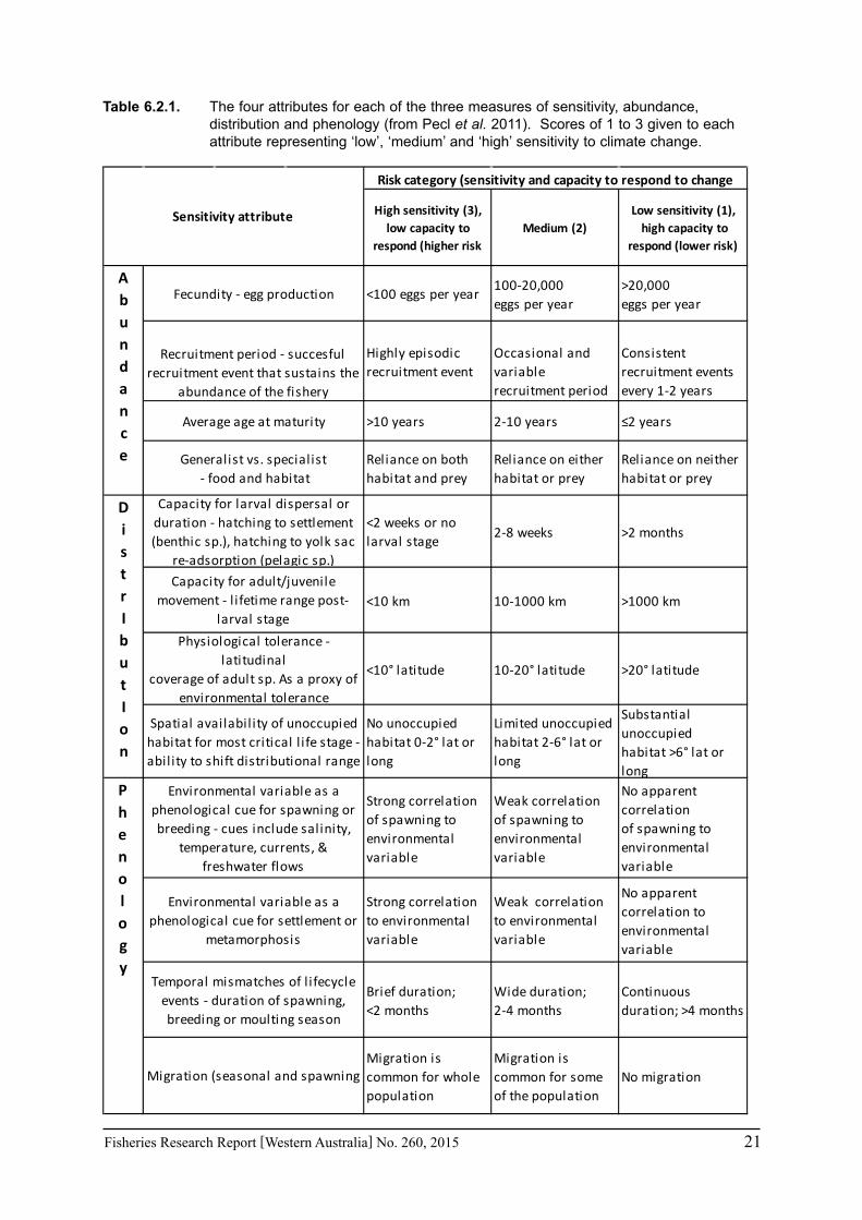
Pecl et al. (2011) determined four attributes for each of the three measures of sensitivity, abundance, distribution and phenology, giving a total for 12 attributes (Table 6.2.1). Scores of 1 to 3 were given to each attribute representing ‘low’, ‘medium’ and ‘high’ sensitivity to climate change. The scores for each group of four attributes were averaged to obtain scores for abundance, distribution and phenology. These three scores were then added to get an assessment of the relative sensitivity of species to climate change across all the measures. The uncertainty associated with any of the assessments such as lack of scientific evidence or data was acknowledged and a pre-cautionary approach was adopted by selecting a ranking on the higher side of the range (i.e. more sensitive to climate change). These scores were based on the available literature information for the species and the expertise of the fisheries scientists and reviewed by other scientists to ensure that the interpretation of the criteria was consistently applied.
The species were then ranked based on their sensitivity to climate change and classified into 5 sensitivity classes: high, medium-high, medium, medium-low and low as undertaken by Pecl et al. (2011). These classes were given a ranking of 5 to 1, respectively, to be used in the estimate of the risk assessment of species to climate change.
The ‘exposure’ (or likelihood component) of the risk assessment was not undertaken by Pecl et al. (2011) as it was not within the scope of their project. This exposure estimate for each
20 Fisheries Research Report [Western Australia] No. 260, 2015
species was based on information on the (a) likely environmental variables that that may affect a species; and (b) historic and projected trends in those environmental variables based on climate change scenarios (Section 7.1). The expected effects of climate changes for key environmental indicators predicted for 2060 for scenario A1B were estimated for the four bioregions of Western Australia as environmental trends can vary greatly between the large latitudinal variations that cover WA. These trends were based on modelling undertaken as part of objective 1 on this study (Section 6.1) or data available in the literature. The four bioregional areas in WA were those used in the ecosystem-based fisheries management approach (Fletcher et al. 2010) representing the north coast, Gascoyne coast, west coast and south coast. A ranking of the exposure (or likelihood) from 1 to 5 is used to represent the classifications from ‘remote’ to ‘certain’ (Table 6.2.2). The ‘sensitivity’ and exposure components can be multiplied to obtain a relative risk ranking for species that may be affected by climate change (Table 6.2.3).
This risk assessment approach provides a comparative basis for identifying species that may have the highest risk of being affected by climate change and a priority for monitoring and further investigation for climate change adaptation which is the third objective of this study. However other socio-economic factors are also relevant to the priority setting process for assessing climate change effects. Therefore it is important to see how the risk assessment for climate change fits in with the risk assessment for the ecosystem-based fisheries management (EBFM) that is conducted at the regional level (Fletcher et al. 2010; 2012) and provides a basis for priority setting for research and management by the Department of Fisheries (DoF) in WA. There are three components of the risk assessment approach which evaluates the ecological risk of species but also takes into account the economic value of the species as well the social amenity (i.e. no-economic benefits) derived by the community (Fletcher et al. 2010; 2012).
The approach adopted for determining priorities for climate change research on species used the following approach as per Fletcher et al. (2010; 2012):
• Classify species into bioregion and asset classification (e.g. finfish broken down by estuarine, inshore demersal, nearshore, offshore demersal and pelagic) (Fletcher et al. 2010); and
• Apply economic and social assessment evaluations (from the DoF risk assessment approach) to the climate change risk of species to identify agency priorities for research/management under climate change.
The climate change risk would therefore be one aspect of the overall priority setting for research and management for the Department of Fisheries in WA.
Fisheries Research Report [Western Australia] No. 260, 2015 21
Table 6.2.1. The four attributes for each of the three measures of sensitivity, abundance, distribution and phenology (from Pecl et al. 2011). Scores of 1 to 3 given to each attribute representing ‘low’, ‘medium’ and ‘high’ sensitivity to climate change.
<100 eggs per year100-20,000eggs per year
>20,000eggs per year
Highly episodicrecruitment event
Occasional and variable recruitment period
Consistentrecruitment events every 1-2 years
>10 years 2-10 years ≤2 years
Reliance on bothhabitat and prey
Reliance on eitherhabitat or prey
Reliance on neitherhabitat or prey
<2 weeks or nolarval stage
2-8 weeks >2 months
<10 km 10-1000 km >1000 km
<10° latitude 10-20° latitude >20° latitude
No unoccupiedhabitat 0-2° lat or long
Limited unoccupiedhabitat 2-6° lat or long
Substantial unoccupiedhabitat >6° lat or long
Strong correlationof spawning to environmental variable
Weak correlationof spawning to environmental variable
No apparent correlationof spawning to environmental variable
Strong correlation to environmental variable
Weak correlation to environmental variable
No apparent correlation to environmental variable
Brief duration;<2 months
Wide duration;2-4 months
Continuousduration; >4 months
Migration is common for whole population
Migration is common for some of the population
No migration
Risk category (sensitivity and capacity to respond to change
Abundance
DistrIbutIon
Sensitivity attribute High sensitivity (3),low capacity to
respond (higher riskMedium (2)
Low sensitivity (1), high capacity to
respond (lower risk)
Fecundity - egg production
Recruitment period - succesfulrecruitment event that sustains the
abundance of the fishery
Average age at maturity
Generalist vs. specialist - food and habitat
Capacity for larval dispersal orduration - hatching to settlement (benthic sp.), hatching to yolk sac
re-adsorption (pelagic sp.)
Capacity for adult/juvenilemovement - l ifetime range post-
larval stage
Physiological tolerance - latitudinal
coverage of adult sp. As a proxy of environmental tolerance
Spatial availabil ity of unoccupiedhabitat for most critical l ife stage - abil ity to shift distributional range
Migration (seasonal and spawning
Phenology
Environmental variable as aphenological cue for spawning or breeding - cues include salinity,
temperature, currents, & freshwater flows
Environmental variable as a phenological cue for settlement or
metamorphosis
Temporal mismatches of l ifecycleevents - duration of spawning, breeding or moulting season
22 Fisheries Research Report [Western Australia] No. 260, 2015
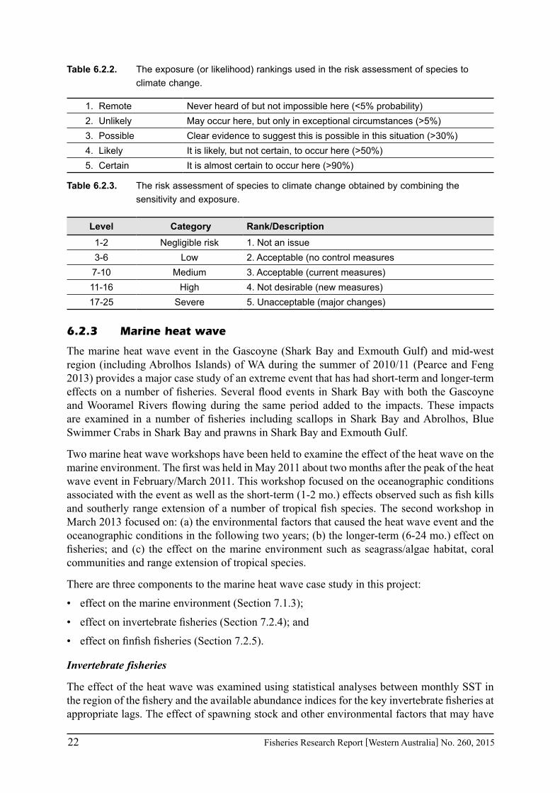
Table 6.2.2. The exposure (or likelihood) rankings used in the risk assessment of species to climate change.
1. Remote Never heard of but not impossible here (<5% probability)2. Unlikely May occur here, but only in exceptional circumstances (>5%)3. Possible Clear evidence to suggest this is possible in this situation (>30%)4. Likely It is likely, but not certain, to occur here (>50%)5. Certain It is almost certain to occur here (>90%)
Table 6.2.3. The risk assessment of species to climate change obtained by combining the sensitivity and exposure.
Level Category Rank/Description1-2 Negligible risk 1. Not an issue3-6 Low 2. Acceptable (no control measures7-10 Medium 3. Acceptable (current measures)11-16 High 4. Not desirable (new measures)17-25 Severe 5. Unacceptable (major changes)
6.2.3 Marine heat wave
The marine heat wave event in the Gascoyne (Shark Bay and Exmouth Gulf) and mid-west region (including Abrolhos Islands) of WA during the summer of 2010/11 (Pearce and Feng 2013) provides a major case study of an extreme event that has had short-term and longer-term effects on a number of fisheries. Several flood events in Shark Bay with both the Gascoyne and Wooramel Rivers flowing during the same period added to the impacts. These impacts are examined in a number of fisheries including scallops in Shark Bay and Abrolhos, Blue Swimmer Crabs in Shark Bay and prawns in Shark Bay and Exmouth Gulf.
Two marine heat wave workshops have been held to examine the effect of the heat wave on the marine environment. The first was held in May 2011 about two months after the peak of the heat wave event in February/March 2011. This workshop focused on the oceanographic conditions associated with the event as well as the short-term (1-2 mo.) effects observed such as fish kills and southerly range extension of a number of tropical fish species. The second workshop in March 2013 focused on: (a) the environmental factors that caused the heat wave event and the oceanographic conditions in the following two years; (b) the longer-term (6-24 mo.) effect on fisheries; and (c) the effect on the marine environment such as seagrass/algae habitat, coral communities and range extension of tropical species.
There are three components to the marine heat wave case study in this project:
• effect on the marine environment (Section 7.1.3);
• effect on invertebrate fisheries (Section 7.2.4); and
• effect on finfish fisheries (Section 7.2.5).
Invertebrate fisheries
The effect of the heat wave was examined using statistical analyses between monthly SST in the region of the fishery and the available abundance indices for the key invertebrate fisheries at appropriate lags. The effect of spawning stock and other environmental factors that may have
Fisheries Research Report [Western Australia] No. 260, 2015 23
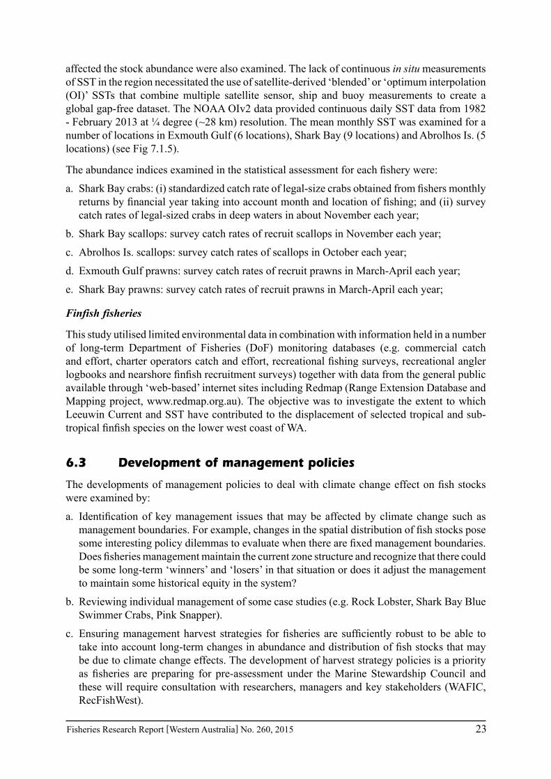
affected the stock abundance were also examined. The lack of continuous in situ measurements of SST in the region necessitated the use of satellite-derived ‘blended’ or ‘optimum interpolation (OI)’ SSTs that combine multiple satellite sensor, ship and buoy measurements to create a global gap-free dataset. The NOAA OIv2 data provided continuous daily SST data from 1982 - February 2013 at ¼ degree (~28 km) resolution. The mean monthly SST was examined for a number of locations in Exmouth Gulf (6 locations), Shark Bay (9 locations) and Abrolhos Is. (5 locations) (see Fig 7.1.5).
The abundance indices examined in the statistical assessment for each fishery were:
a. Shark Bay crabs: (i) standardized catch rate of legal-size crabs obtained from fishers monthly returns by financial year taking into account month and location of fishing; and (ii) survey catch rates of legal-sized crabs in deep waters in about November each year;
b. Shark Bay scallops: survey catch rates of recruit scallops in November each year;
c. Abrolhos Is. scallops: survey catch rates of scallops in October each year;
d. Exmouth Gulf prawns: survey catch rates of recruit prawns in March-April each year;
e. Shark Bay prawns: survey catch rates of recruit prawns in March-April each year;
Finfish fisheries
This study utilised limited environmental data in combination with information held in a number of long-term Department of Fisheries (DoF) monitoring databases (e.g. commercial catch and effort, charter operators catch and effort, recreational fishing surveys, recreational angler logbooks and nearshore finfish recruitment surveys) together with data from the general public available through ‘web-based’ internet sites including Redmap (Range Extension Database and Mapping project, www.redmap.org.au). The objective was to investigate the extent to which Leeuwin Current and SST have contributed to the displacement of selected tropical and sub-tropical finfish species on the lower west coast of WA.
6.3 Development of management policies
The developments of management policies to deal with climate change effect on fish stocks were examined by:
a. Identification of key management issues that may be affected by climate change such as management boundaries. For example, changes in the spatial distribution of fish stocks pose some interesting policy dilemmas to evaluate when there are fixed management boundaries. Does fisheries management maintain the current zone structure and recognize that there could be some long-term ‘winners’ and ‘losers’ in that situation or does it adjust the management to maintain some historical equity in the system?
b. Reviewing individual management of some case studies (e.g. Rock Lobster, Shark Bay Blue Swimmer Crabs, Pink Snapper).
c. Ensuring management harvest strategies for fisheries are sufficiently robust to be able to take into account long-term changes in abundance and distribution of fish stocks that may be due to climate change effects. The development of harvest strategy policies is a priority as fisheries are preparing for pre-assessment under the Marine Stewardship Council and these will require consultation with researchers, managers and key stakeholders (WAFIC, RecFishWest).

24 Fisheries Research Report [Western Australia] No. 260, 2015
The reduced recruitment to the Western Rock Lobster fishery over seven years and the effect of the 2010/11 marine heat wave on the abalone, scallop, crabs, prawn and finfish stocks in the Gascoyne and mid-west have provided real examples of a long-term change in a fishery and an extreme event. The Western Rock Lobster and the effect of the heat wave on invertebrate and finfish fisheries are treated as major case studies that have required research, management and industry to adapt to major changes that are occurring in these fisheries.
The risk assessment of species and the priority-setting process that identifies the fisheries that have the highest priority with respect to climate change issues will also inform the management priorities.
Fisheries Research Report [Western Australia] No. 260, 2015 25
7.0 Results/Discussion
7.1 Climate change effects on marine environment
7.1.1 Historic climate change trends
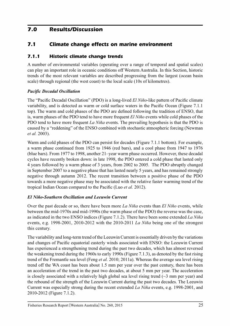
A number of environmental variables (operating over a range of temporal and spatial scales) can play an important role in oceanic conditions off Western Australia. In this Section, historic trends of the most relevant variables are described progressing from the largest (ocean basin scale) through regional (the west coast) to the local scale (10s of kilometres).
Pacific Decadal Oscillation
The “Pacific Decadal Oscillation” (PDO) is a long-lived El Niño-like pattern of Pacific climate variability, and is detected as warm or cold surface waters in the Pacific Ocean (Figure 7.1.1 top). The warm and cold phases of the PDO are defined following the tradition of ENSO, that is, warm phases of the PDO tend to have more frequent El Niño events while cold phases of the PDO tend to have more frequent La Niña events. The prevailing hypothesis is that the PDO is caused by a “reddening” of the ENSO combined with stochastic atmospheric forcing (Newman et al. 2003).
Warm and cold phases of the PDO can persist for decades (Figure 7.1.1 bottom). For example, a warm phase continued from 1925 to 1946 (red bars), and a cool phase from 1947 to 1976 (blue bars). From 1977 to 1998, another 21–year warm phase occurred. However, these decadal cycles have recently broken down: in late 1998, the PDO entered a cold phase that lasted only 4 years followed by a warm phase of 3 years, from 2002 to 2005. The PDO abruptly changed in September 2007 to a negative phase that has lasted nearly 5 years, and has remained strongly negative through autumn 2012. The recent transition between a positive phase of the PDO towards a more negative phase may be associated with the relative faster warming trend of the tropical Indian Ocean compared to the Pacific (Luo et al. 2012).
El Niño-Southern Oscillation and Leeuwin Current
Over the past decade or so, there have been more La Niña events than El Niño events, while between the mid-1970s and mid-1990s (the warm phase of the PDO) the reverse was the case, as indicated in the two ENSO indices (Figure 7.1.2). There have been some extended La Niña events, e.g. 1998-2001, 2010-2012 with the 2010-2011 La Niña being one of the strongest this century.
The variability and long-term trend of the Leeuwin Current is essentially driven by the variations and changes of Pacific equatorial easterly winds associated with ENSO: the Leeuwin Current has experienced a strengthening trend during the past two decades, which has almost reversed the weakening trend during the 1960s to early 1990s (Figure 7.1.3), as denoted by the fast rising trend of the Fremantle sea level (Feng et al. 2010; 2011a). Whereas the average sea level rising trend off the WA coast has been about 1.5 mm per year over the past century, there has been an acceleration of the trend in the past two decades, at about 5 mm per year. The acceleration is closely associated with a relatively high global sea level rising trend (~3 mm per year) and the rebound of the strength of the Leeuwin Current during the past two decades. The Leeuwin Current was especially strong during the recent extended La Niña events, e.g. 1998-2001, and 2010-2012 (Figure 7.1.2).

26 Fisheries Research Report [Western Australia] No. 260, 2015
Figure 7.1.1. (Top) Sea surface temperature anomaly pattern during a positive (warm) phase of the PDO. (Bottom) Average Pacific Decadal Oscillation (PDO) index during the northern hemisphere summer. (http://www.nwfsc.noaa.gov/research/divisions/fe/estuarine/oeip/ca-pdo.cfm, accessed on 2 May 2013).

Fisheries Research Report [Western Australia] No. 260, 2015 27
Figure 7.1.2. (a) Niño 3.4 area sea surface temperature (SST) and Southern Oscillation Index (scaled down by factor of 10). (b) zonal wind stress anomalies averaged over 3°S – 3°N, 130 – 160°E in the equatorial Pacific, where the zonal wind anomalies lead the Fremantle sea level (FSL) on interannual time scales, and meridional wind stress anomalies off the west coast of Australia averaged over 30–22°S, 110–116°E, as derived from the Tropflux product. (c) FSL anomalies, as an index of the strength of the Leeuwin Current. (d) SST anomalies averaged over 32–26°S, 112–115°E off the west coast of Australia (where the interannual temperature variation is largely responding to the Leeuwin Current heat transport), derived from the OISST. (e) Upper ocean (0–150 m) heat content anomalies off northwest Australia (22–15°S, 108–114°E), the key forcing region of the Leeuwin Current, derived from GODAS reanalysis. The heavy contours denote the 20°C and 25°C isothermal depths. The red curve in d is derived from TMI SST product. Anomalies in b, c, d and e are smoothed with a 5-point Hanning filter. A linear trend of 1.6 mm per year has been removed from the FSL to account for the global sea level rising trend during the past century (from Feng et al. 2013).

28 Fisheries Research Report [Western Australia] No. 260, 2015
Figure 7.1.3. Low-passed filtered sea levels in the eastern (region A) and western Pacific (region B) and their relations with the Fremantle sea level (adapted from Feng et al. 2010). Fremantle sea level has been used as an index of the strength of the Leeuwin Current.
Decadal-scale changes in the SOI and Fremantle sea level can be traced back over a century, largely reflecting the occurrence, persistence and intensity of El Niño and La Niña events during each decade. While for much of the past century the decadal SOI was small, indicative of decade-neutral conditions (Figure 7.1.4c), the 1920s and 1970s were both periods with elevated values of the SOI whereas the 2-decadal period 1981 to 2000 experienced stronger El Niño-like conditions (lower SOIs). The relative frequencies of El Niño and La Niña conditions during each decade depend on the SOI thresholds used to define such events. For example, using moderate SOI levels <-10 or >+10 (Figure 7.1.5a) indicates that the decades 1911 and 1981 to 2001 all experienced more moderate El Niño events compared with La Niña events while the reverse was the case in the 1970s. For the extreme events with SOI<-20 and >+20 (Figure 7.1.5b), the 1980s and 1990s stand out as being dominated by very strong El Niño conditions whereas the 2001 decade saw more La Niña events.
Sea level off the west coast has shown a generally steady rise of about 16 cm over the past century, although the rate of rise has not been constant (Figure 7.1.4a). In particular, there was a small fall in sea level in the 2 decades 1911–1920 (-1.05 cm) and 1981–1990 (-0.79 cm). Each of these was followed by a decade of accelerated sea level rise. The decadal standard deviations (Figure 7.1.4b) indicate that sea level variability was also high during the 1911–1920 period and relatively low between 1981 and 1990, but was otherwise fairly uniform.

Fisheries Research Report [Western Australia] No. 260, 2015 29
50
60
70
80
1901 1911 1921 1931 1941 1951 1961 1971 1981 1991 2001
a) Decadal FMSL (cm)
0
5
10
15
20
1901 1911 1921 1931 1941 1951 1961 1971 1981 1991 2001
b) Decadal FMSL Stdev (cm)
-5
0
5
1901 1911 1921 1931 1941 1951 1961 1971 1981 1991 2001
c) Decadal SOI
0
5
10
15
20
1901 1911 1921 1931 1941 1951 1961 1971 1981 1991 2001
d) Decadal SOI StDev SOI
Figure 7.1.4. Decadal averages in (a) Fremantle sea level over the past century and (b) variability (represented by the decadal standard deviations), and the corresponding plots for the Southern Oscillation Index (SOI, c and d). In each case, the decade runs from e.g. 1901 to 1910. The values have been derived from the monthly mean sea levels and SOIs.

30 Fisheries Research Report [Western Australia] No. 260, 2015
a)
0
10
20
30
40
1901 1911 1921 1931 1941 1951 1961 1971 1981 1991 2001
El Nino La Nina
b)
0
10
1901 1911 1921 1931 1941 1951 1961 1971 1981 1991 2001
El Nino La Nina
Figure 7.1.5. Relative decadal frequencies (measured by number of months) of El Niño (blue) and La Niña (red) events as defined by (a) SOIs with a threshold of 10 and (b) more extreme events with SOIs threshold of 20.
SST and sea surface salinity
The ocean off the southwest of Western Australia is observed to be one of three “hot spots” in the Indian Ocean where the rising trends of sea surface temperature since the 1950s are higher than the Indian Ocean basin average (Figure 7.1.6; Pearce and Feng 2007). Depth-averaged temperature records at the CSIRO Rottnest 50m station have revealed an increase of ~0.6°C since the 1950s. There are lower rising trends in surface temperatures off the northwest (e.g. Lough 2008) and south coasts of Australia. Over the past 30 years, surface temperature increases have mostly occurred in autumn-winter off the west coast, at about 0.02–0.035°C per year, compared to little or no increase (<0.01°C per year) in the spring-summer period (Caputi et al. 2009). This has caused a delay in seasonal cycles of surface temperatures off the west coast by 10–20 days. Despite the stronger autumn-winter trend of ocean surface temperatures off the west coast, most of the surface temperature variability occurs in summer during seasonally phase-locked warming and cooling events off the coast (Kataoka et al. 2013). It is not clear yet if the recent consecutive marine heat waves in summer represent a long-term trend or are simply due to the phase transition of the PDO.
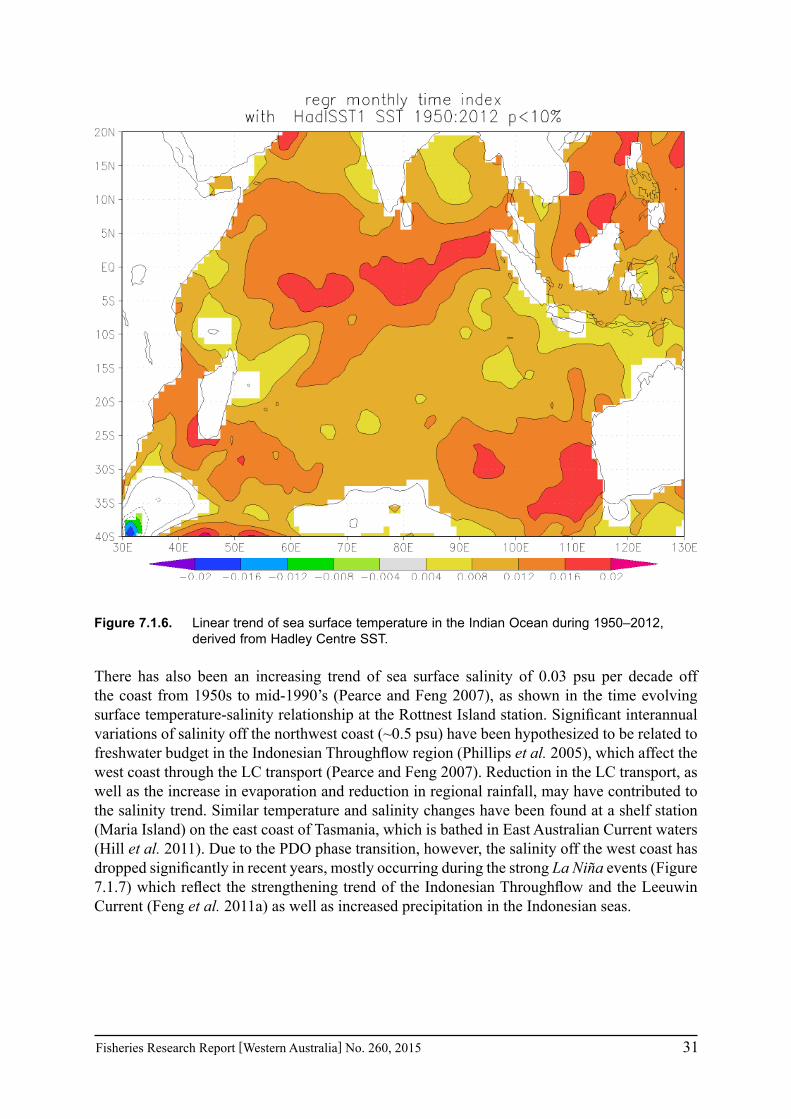
Fisheries Research Report [Western Australia] No. 260, 2015 31
Figure 7.1.6. Linear trend of sea surface temperature in the Indian Ocean during 1950–2012, derived from Hadley Centre SST.
There has also been an increasing trend of sea surface salinity of 0.03 psu per decade off the coast from 1950s to mid-1990’s (Pearce and Feng 2007), as shown in the time evolving surface temperature-salinity relationship at the Rottnest Island station. Significant interannual variations of salinity off the northwest coast (~0.5 psu) have been hypothesized to be related to freshwater budget in the Indonesian Throughflow region (Phillips et al. 2005), which affect the west coast through the LC transport (Pearce and Feng 2007). Reduction in the LC transport, as well as the increase in evaporation and reduction in regional rainfall, may have contributed to the salinity trend. Similar temperature and salinity changes have been found at a shelf station (Maria Island) on the east coast of Tasmania, which is bathed in East Australian Current waters (Hill et al. 2011). Due to the PDO phase transition, however, the salinity off the west coast has dropped significantly in recent years, mostly occurring during the strong La Niña events (Figure 7.1.7) which reflect the strengthening trend of the Indonesian Throughflow and the Leeuwin Current (Feng et al. 2011a) as well as increased precipitation in the Indonesian seas.

32 Fisheries Research Report [Western Australia] No. 260, 2015
Figure 7.1.7. Sea surface salinity averaged over 33-31ºS, 114-116ºE from EN3 objective analysis data developed by Ingleby et al. (2007)
Rainfall
While the Indian Ocean Climate Initiative (IOCI) research suggested that the late 1960s rainfall decline for southwest WA occurred in early winter, primarily on the west coast; rainfall declines are now evident across all of the southwest (IOCI 2012). A further rainfall downturn appeared to take place in the late 1990s. The large-scale circulation and local weather patterns match this rainfall decline – July storms are less common due to fewer low-pressure systems and more high-pressure systems and these observed circulation changes are also reflected in climate model projects – increasing levels of greenhouse gases in the atmosphere are likely to have contributed to the rainfall decline, and land clearing may also have played a role.
IOCI research also suggests that the number of tropical cyclones will be 50% fewer in future and so a decrease in rainfall is expected, however, the cyclones are likely to be more intense. There is an increasing trend in rainfall currently occurring which may be due to an increase in aerosols, and the predicted decrease assumes future reductions in aerosols (IOCI 2012).
7.1.2 Marine heat wave – Ningaloo Niño
During the February/March 2011 marine heat wave, nearshore water temperatures along the Gascoyne and mid-west coast exceeded 5°C above the long-term average for brief periods. This has been attributed to both the very strong Leeuwin Current (anomalously high coastal sea levels) during the intense La Niña period described above and anomalously high air-sea heat flux entering the ocean (Pearce and Feng 2013). Effects on the marine biota were devastating, with massive mortality in some areas, while there were also sightings of tropical species (including some iconic megafauna) well south of their normal ranges (Pearce et al. 2011 – also Sections 7.2.4 and 7.2.5).

Fisheries Research Report [Western Australia] No. 260, 2015 33
Unusually warm water was also encountered during the summers of 2011/12 and 2012/13, and the biological consequences of this are presently being analysed (Caputi et al. 2014d).
The close relationships between the monthly SOI, Fremantle sea level and SST that have been discussed in the previous section, are clearly evident over the past 3 decades (Figure 7.1.8a). The major El Niño events (1982/83, 1987, early 1992 and 1997/98) were all associated with lower sea levels (weaker Leeuwin Current) and cooler water, while during the strong La Niña periods (1988/89, 1998–2000, 2008/09 and 2010–12) higher sea levels indicated that the Leeuwin Current was flowing strongly and water temperatures were relatively high. There were occasions (such as 1994/95 and 1997) when the water was warmer despite lower sea levels and El Niño-like conditions, suggesting that other drivers such as air-sea heat flux (acting independently of the Leeuwin Current) also play an important role in influencing local ocean temperatures.
a)
-30
-20
-10
0
10
20
30
1980 1985 1990 1995 2000 2005 2010Year
SOI;
FM
SL (c
m)
-3
-2
-1
0
1
2
3
Rey
nSST
Ano
m (°
C)
FMSL anomalySOIReynoldsSST anomaly °C
b)
-30
-20
-10
0
10
20
30
2004 2005 2006 2007 2008 2009 2010 2011 2012 2013Year
SOI;
FM
SL (c
m)
-3
-2
-1
0
1
2
3R
eynS
STA
nom
(°C
)FMSL anomalySOIReynoldsSST anomaly °C
Figure 7.1.8. Monthly values of the Southern Oscillation Index (black), the anomaly of Fremantle sea level (blue) and the anomaly of sea-surface temperature at the Abrolhos Islands (SST, red) between (a) 1980 and early 2013, and (b) over the last decade. The anomalies have been derived by subtracting the long-term mean annual cycle from the individual monthly values, and have been smoothed by a 3-month moving average to reduce small-scale variability and highlight the dominant relationships (Pearce et al. in prep.).

34 Fisheries Research Report [Western Australia] No. 260, 2015
The monthly Reynolds SSTs for the summer months over the past 3 decades showed both the intensity and the regional (alongshore) variability of the heat wave (Figure 7.1.9a). The water was warmest at 2-3°C above the long-term monthly average for all the west coast locations in early 2011 while the south coast was about 1°C above average (Figure 7.1.9b). The elevated temperatures persisted into the summer 2012/13 with Ningaloo, Albany and Esperance recording their highest summer temperatures.
a) Summer Temperatures
18
20
22
24
26
28
30
1982 1987 1992 1997 2002 2007 2012
Year
Tem
pera
ture
°C
Ning ShBay Abr RotCapes Alb Esp
b) Summer Temperature Anomalies
-2
-1
0
1
2
3
1982 1987 1992 1997 2002 2007 2012
Year
Tem
pera
ture
Ano
mal
y °C
Ning ShBay Abr RotCapes Alb Esp
Figure 7.1.9. (a) Summer water temperatures from the Reynolds SST dataset for the 1-degree blocks off Ningaloo, Shark Bay, the Abrolhos Islands, Rottnest Island, the Capes region, Albany and Esperance. (b) Summer temperature anomalies from the long-term annual cycle. Summer is defined as December-January-February.
These larger-scale (monthly, 100-km block averages) SSTs in early 2011 were at record levels. On a more local scale, the hourly temperature logger measurements from the nearshore and island locations over the past decade revealed the even more extreme conditions near the coast. The peak daily temperature anomalies at Rat Island, Dongara, Rottnest Island, Warnbro Sound and Busselton Jetty (representing both coastal and outer shelf conditions) showed that local water temperatures during summer 2010/11 peaked at ~5°C above the long-term average between the Abrolhos Islands and Jurien (Table 7.1.1).
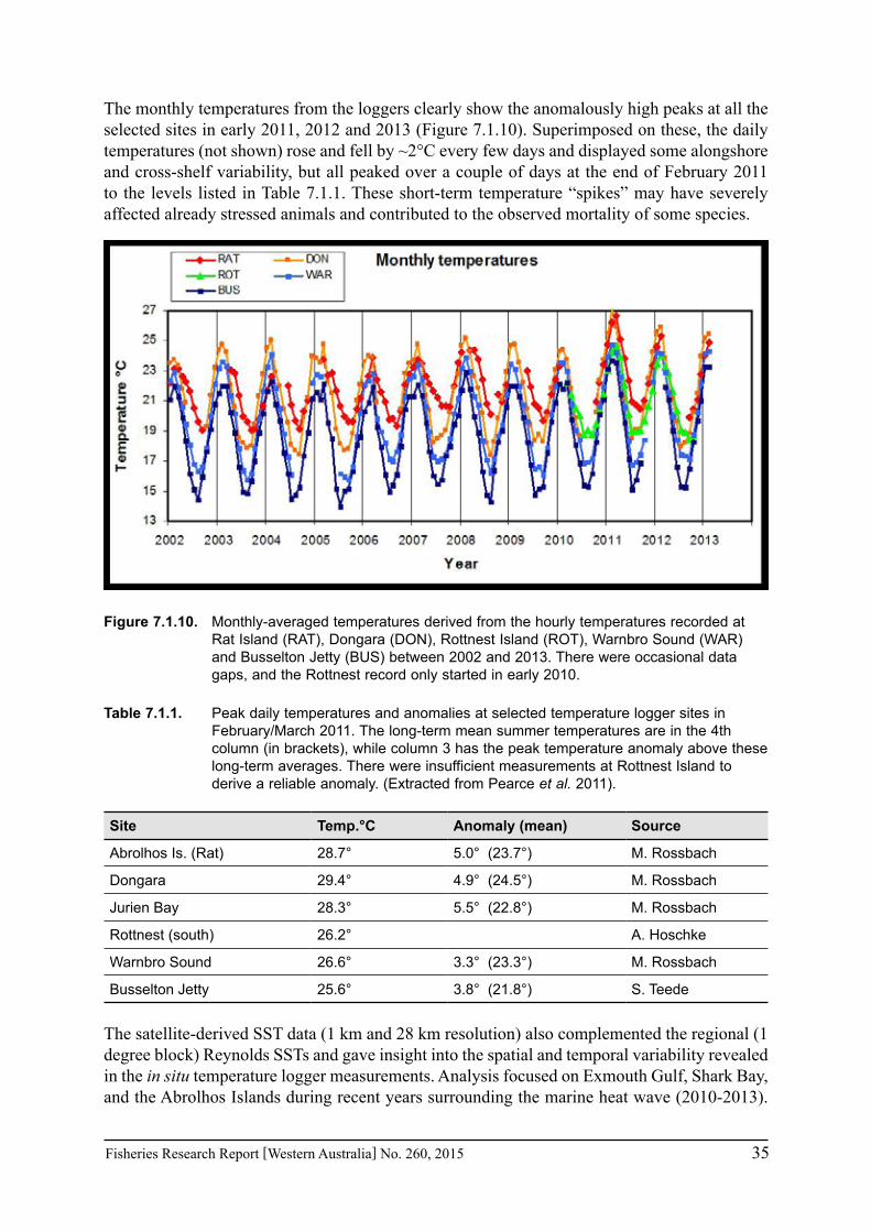
Fisheries Research Report [Western Australia] No. 260, 2015 35
The monthly temperatures from the loggers clearly show the anomalously high peaks at all the selected sites in early 2011, 2012 and 2013 (Figure 7.1.10). Superimposed on these, the daily temperatures (not shown) rose and fell by ~2°C every few days and displayed some alongshore and cross-shelf variability, but all peaked over a couple of days at the end of February 2011 to the levels listed in Table 7.1.1. These short-term temperature “spikes” may have severely affected already stressed animals and contributed to the observed mortality of some species.
Figure 7.1.10. Monthly-averaged temperatures derived from the hourly temperatures recorded at Rat Island (RAT), Dongara (DON), Rottnest Island (ROT), Warnbro Sound (WAR) and Busselton Jetty (BUS) between 2002 and 2013. There were occasional data gaps, and the Rottnest record only started in early 2010.
Table 7.1.1. Peak daily temperatures and anomalies at selected temperature logger sites in February/March 2011. The long-term mean summer temperatures are in the 4th column (in brackets), while column 3 has the peak temperature anomaly above these long-term averages. There were insufficient measurements at Rottnest Island to derive a reliable anomaly. (Extracted from Pearce et al. 2011).
Site Temp.°C Anomaly (mean) Source
Abrolhos Is. (Rat) 28.7° 5.0° (23.7°) M. Rossbach
Dongara 29.4° 4.9° (24.5°) M. Rossbach
Jurien Bay 28.3° 5.5° (22.8°) M. Rossbach
Rottnest (south) 26.2° A. Hoschke
Warnbro Sound 26.6° 3.3° (23.3°) M. Rossbach
Busselton Jetty 25.6° 3.8° (21.8°) S. Teede
The satellite-derived SST data (1 km and 28 km resolution) also complemented the regional (1 degree block) Reynolds SSTs and gave insight into the spatial and temporal variability revealed in the in situ temperature logger measurements. Analysis focused on Exmouth Gulf, Shark Bay, and the Abrolhos Islands during recent years surrounding the marine heat wave (2010-2013).
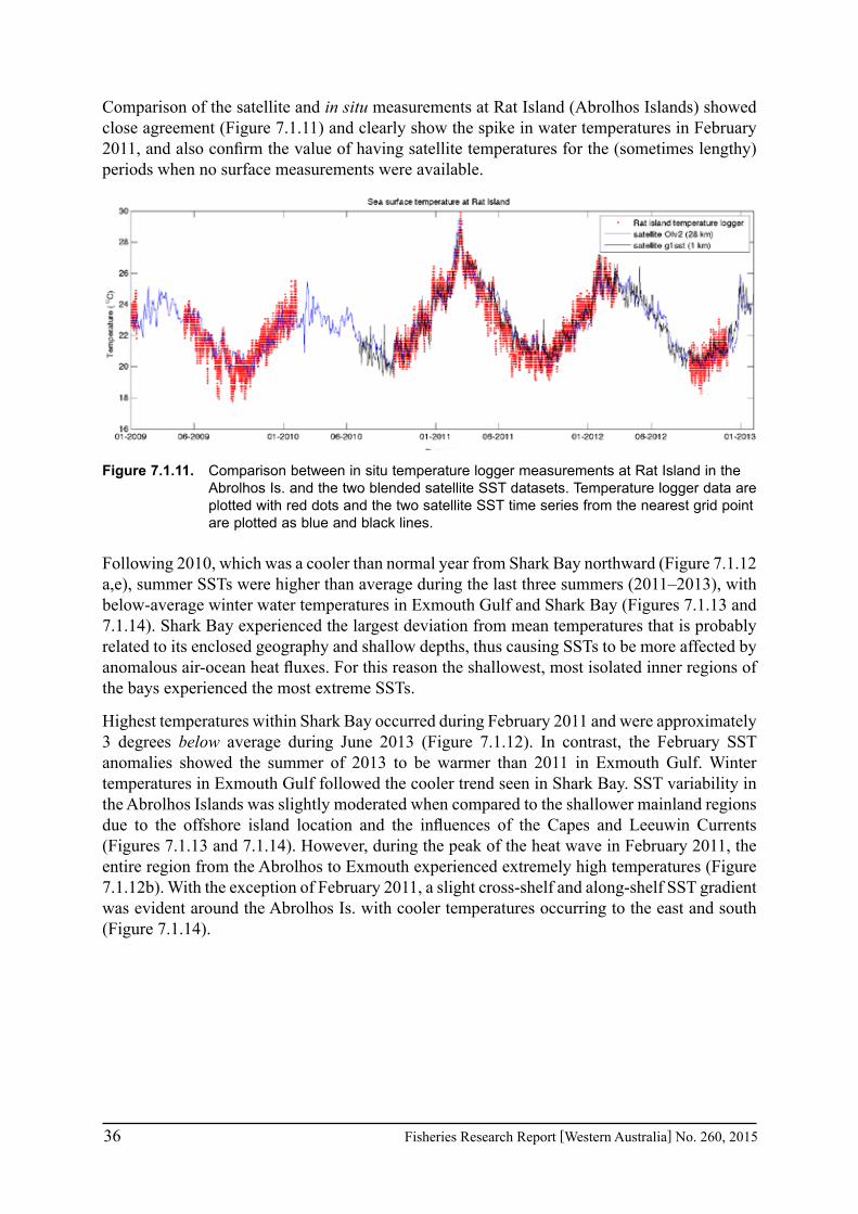
36 Fisheries Research Report [Western Australia] No. 260, 2015
Comparison of the satellite and in situ measurements at Rat Island (Abrolhos Islands) showed close agreement (Figure 7.1.11) and clearly show the spike in water temperatures in February 2011, and also confirm the value of having satellite temperatures for the (sometimes lengthy) periods when no surface measurements were available.
Figure 7.1.11. Comparison between in situ temperature logger measurements at Rat Island in the Abrolhos Is. and the two blended satellite SST datasets. Temperature logger data are plotted with red dots and the two satellite SST time series from the nearest grid point are plotted as blue and black lines.
Following 2010, which was a cooler than normal year from Shark Bay northward (Figure 7.1.12 a,e), summer SSTs were higher than average during the last three summers (2011–2013), with below-average winter water temperatures in Exmouth Gulf and Shark Bay (Figures 7.1.13 and 7.1.14). Shark Bay experienced the largest deviation from mean temperatures that is probably related to its enclosed geography and shallow depths, thus causing SSTs to be more affected by anomalous air-ocean heat fluxes. For this reason the shallowest, most isolated inner regions of the bays experienced the most extreme SSTs.
Highest temperatures within Shark Bay occurred during February 2011 and were approximately 3 degrees below average during June 2013 (Figure 7.1.12). In contrast, the February SST anomalies showed the summer of 2013 to be warmer than 2011 in Exmouth Gulf. Winter temperatures in Exmouth Gulf followed the cooler trend seen in Shark Bay. SST variability in the Abrolhos Islands was slightly moderated when compared to the shallower mainland regions due to the offshore island location and the influences of the Capes and Leeuwin Currents (Figures 7.1.13 and 7.1.14). However, during the peak of the heat wave in February 2011, the entire region from the Abrolhos to Exmouth experienced extremely high temperatures (Figure 7.1.12b). With the exception of February 2011, a slight cross-shelf and along-shelf SST gradient was evident around the Abrolhos Is. with cooler temperatures occurring to the east and south (Figure 7.1.14).

Fisheries Research Report [Western Australia] No. 260, 2015 37
Figure 7.1.12. Monthly mean SST anomalies calculated from the ¼ degree (28 km) resolution OIv2 dataset. Colours represent degrees above/below the 1982-2012 mean temperatures for February (a-d) and June (e-h) and temperature contours are shown at 0.5 degree intervals. The locations of time-series extracted for Figure 7.1.13 are shown in (a).
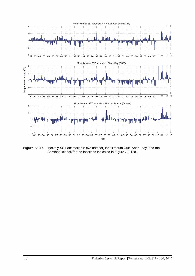
38 Fisheries Research Report [Western Australia] No. 260, 2015
Figure 7.1.13. Monthly SST anomalies (OIv2 dataset) for Exmouth Gulf, Shark Bay, and the Abrolhos Islands for the locations indicated in Figure 7.1.12a.
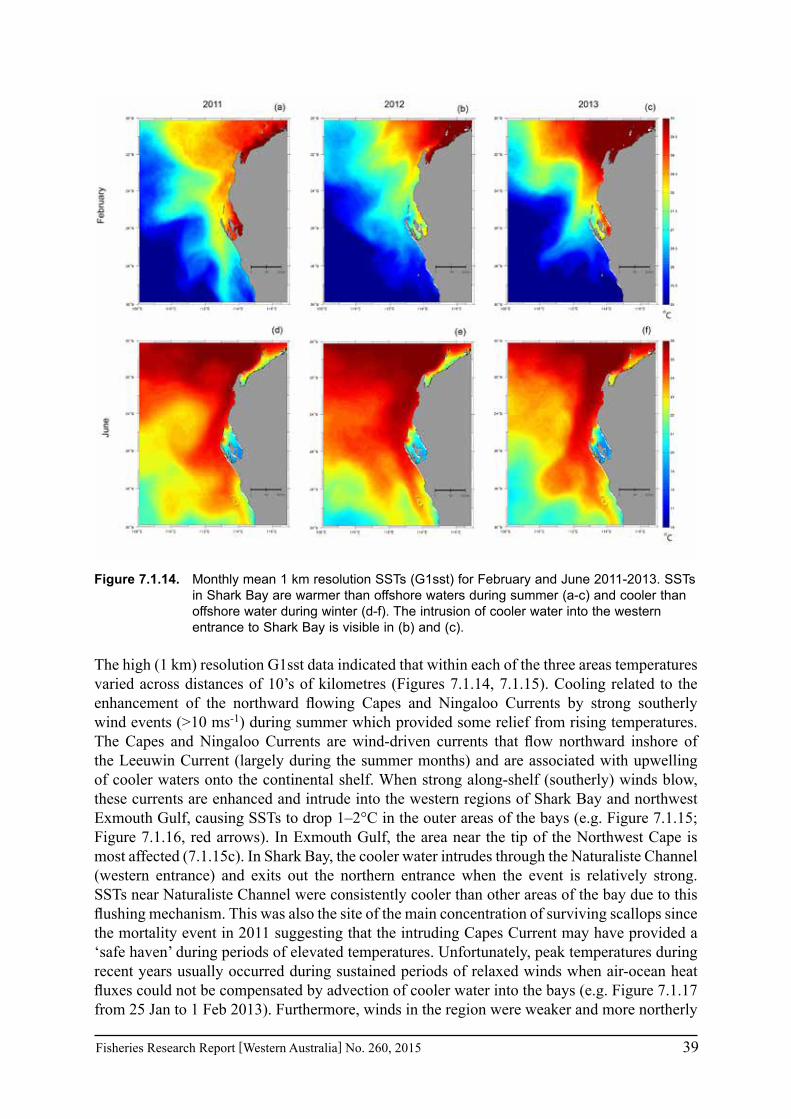
Fisheries Research Report [Western Australia] No. 260, 2015 39
Figure 7.1.14. Monthly mean 1 km resolution SSTs (G1sst) for February and June 2011-2013. SSTs in Shark Bay are warmer than offshore waters during summer (a-c) and cooler than offshore water during winter (d-f). The intrusion of cooler water into the western entrance to Shark Bay is visible in (b) and (c).
The high (1 km) resolution G1sst data indicated that within each of the three areas temperatures varied across distances of 10’s of kilometres (Figures 7.1.14, 7.1.15). Cooling related to the enhancement of the northward flowing Capes and Ningaloo Currents by strong southerly wind events (>10 ms-1) during summer which provided some relief from rising temperatures. The Capes and Ningaloo Currents are wind-driven currents that flow northward inshore of the Leeuwin Current (largely during the summer months) and are associated with upwelling of cooler waters onto the continental shelf. When strong along-shelf (southerly) winds blow, these currents are enhanced and intrude into the western regions of Shark Bay and northwest Exmouth Gulf, causing SSTs to drop 1–2°C in the outer areas of the bays (e.g. Figure 7.1.15; Figure 7.1.16, red arrows). In Exmouth Gulf, the area near the tip of the Northwest Cape is most affected (7.1.15c). In Shark Bay, the cooler water intrudes through the Naturaliste Channel (western entrance) and exits out the northern entrance when the event is relatively strong. SSTs near Naturaliste Channel were consistently cooler than other areas of the bay due to this flushing mechanism. This was also the site of the main concentration of surviving scallops since the mortality event in 2011 suggesting that the intruding Capes Current may have provided a ‘safe haven’ during periods of elevated temperatures. Unfortunately, peak temperatures during recent years usually occurred during sustained periods of relaxed winds when air-ocean heat fluxes could not be compensated by advection of cooler water into the bays (e.g. Figure 7.1.17 from 25 Jan to 1 Feb 2013). Furthermore, winds in the region were weaker and more northerly

40 Fisheries Research Report [Western Australia] No. 260, 2015
during strong La Niña conditions. Wind records from Carnarvon indicated that during the summer of 2010/11 the mean November-March southerly wind component was ~2 ms-1 lower than the long-term mean. Although this was just one of the factors contributing to the high SSTs experienced during the ‘marine heat wave’ it highlights the importance of the wind in controlling water temperatures in these shallow regions.
Figure 7.1.15. Daily SSTs (1 km G1sst) at (a) the Abrolhos Is. (b) Shark Bay and (c) Exmouth Gulf during periods of enhanced Capes (a,b) and Ningaloo Currents (c) during January 2013. The intrusion of cooler water into Shark Bay and northwest Exmouth Gulf is shown with curved black arrows in (b) and (c). White areas are masked either due to cloud cover or proximity to land.
Figure 7.1.16. Smoothed (6 day) sea surface temperature time series extracted from the 1 km G1SST dataset for fisheries survey sites (indicated in Figure 7.1.15) in Exmouth Gulf (blues), Shark Bay (yellows), and the Abrolhos Islands (reds). Red arrows indicate cooling events due to strong southerly winds and enhancement of the Capes and Ningaloo Currents. Summer temperatures within Shark Bay vary by approximately 2°C (a) depending on location and > 4 °C in winter (b). The cooling event during January 2013 corresponds with the intrusion of water into Shark Bay indicated in Figure 7.1.15b.
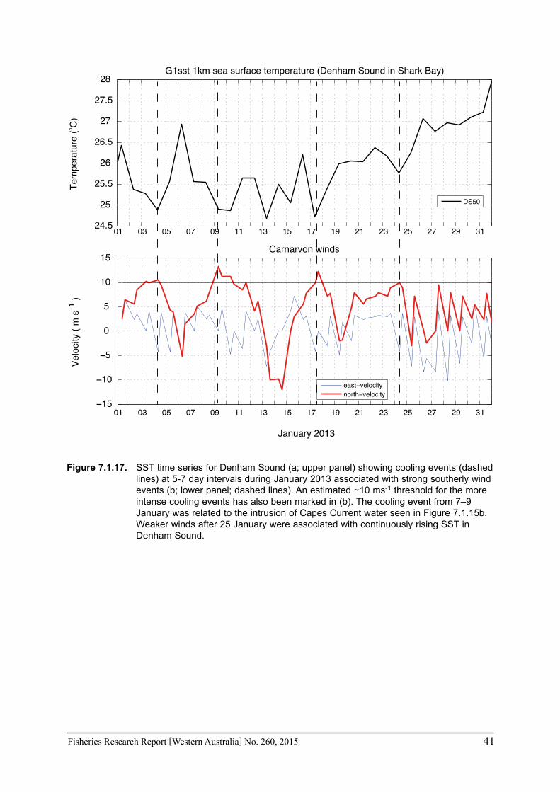
Fisheries Research Report [Western Australia] No. 260, 2015 41
Figure 7.1.17. SST time series for Denham Sound (a; upper panel) showing cooling events (dashed lines) at 5-7 day intervals during January 2013 associated with strong southerly wind events (b; lower panel; dashed lines). An estimated ~10 ms-1 threshold for the more intense cooling events has also been marked in (b). The cooling event from 7–9 January was related to the intrusion of Capes Current water seen in Figure 7.1.15b. Weaker winds after 25 January were associated with continuously rising SST in Denham Sound.

42 Fisheries Research Report [Western Australia] No. 260, 2015
Table 7.1.2. Summary of historic trends in oceanographic variables over the period specified.
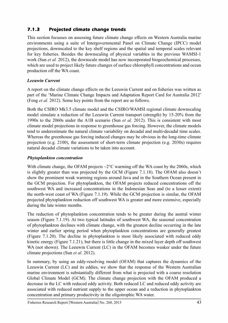
Fisheries Research Report [Western Australia] No. 260, 2015 43
7.1.3 Projected climate change trends
This section focusses on assessing future climate change effects on Western Australia marine environments using a suite of Intergovernmental Panel on Climate Change (IPCC) model projections, downscaled to the key shelf regions and the spatial and temporal scales relevant for key fisheries. Besides the downscaling of physical variables in the previous WAMSI-1 work (Sun et al. 2012), the downscale model has now incorporated biogeochemical processes, which are used to project likely future changes of surface chlorophyll concentrations and ocean production off the WA coast.
Leeuwin Current
A report on the climate change effects on the Leeuwin Current and on fisheries was written as part of the ‘Marine Climate Change Impacts and Adaptation Report Card for Australia 2012’ (Feng et al. 2012). Some key points from the report are as follows.
Both the CSIRO Mk3.5 climate model and the CSIRO/WAMSI regional climate downscaling model simulate a reduction of the Leeuwin Current transport (strength) by 15-20% from the 1990s to the 2060s under the A1B scenario (Sun et al. 2012). This is consistent with most climate model projections in response to greenhouse gas forcing. However, the climate models tend to underestimate the natural climate variability on decadal and multi-decadal time scales. Whereas the greenhouse gas forcing induced changes may be obvious in the long-time climate projection (e.g. 2100), the assessment of short-term climate projection (e.g. 2030s) requires natural decadal climate variations to be taken into account.
Phytoplankton concentration
With climate change, the OFAM projects ~2°C warming off the WA coast by the 2060s, which is slightly greater than was projected by the GCM (Figure 7.1.18). The OFAM also doesn’t show the prominent weak warming regions around Java and in the Southern Ocean present in the GCM projection. For phytoplankton, the OFAM projects reduced concentrations off the southwest WA and increased concentrations in the Indonesian Seas and (to a lesser extent) the north-west coast of WA (Figure 7.1.19). While the GCM projection is similar, the OFAM projected phytoplankton reduction off southwest WA is greater and more extensive, especially during the late winter months.
The reduction of phytoplankton concentration tends to be greater during the austral winter season (Figure 7.1.19). At two typical latitudes of southwest WA, the seasonal concentration of phytoplankton declines with climate change, with the greatest decline occurring in the late winter and earlier spring period when phytoplankton concentrations are generally greatest (Figure 7.1.20). The decline in phytoplankton is most likely associated with reduced eddy kinetic energy (Figure 7.1.21), but there is little change in the mixed layer depth off southwest WA (not shown). The Leeuwin Current (LC) in the OFAM becomes weaker under the future climate projections (Sun et al. 2012).
In summary, by using an eddy-resolving model (OFAM) that captures the dynamics of the Leeuwin Current (LC) and its eddies, we show that the response of the Western Australian marine environment is substantially different from what is projected with a coarse resolution Global Climate Model (GCM). The climate change projection with the OFAM produced a decrease in the LC with reduced eddy activity. Both reduced LC and reduced eddy activity are associated with reduced nutrient supply to the upper ocean and a reduction in phytoplankton concentration and primary productivity in the oligotrophic WA water.
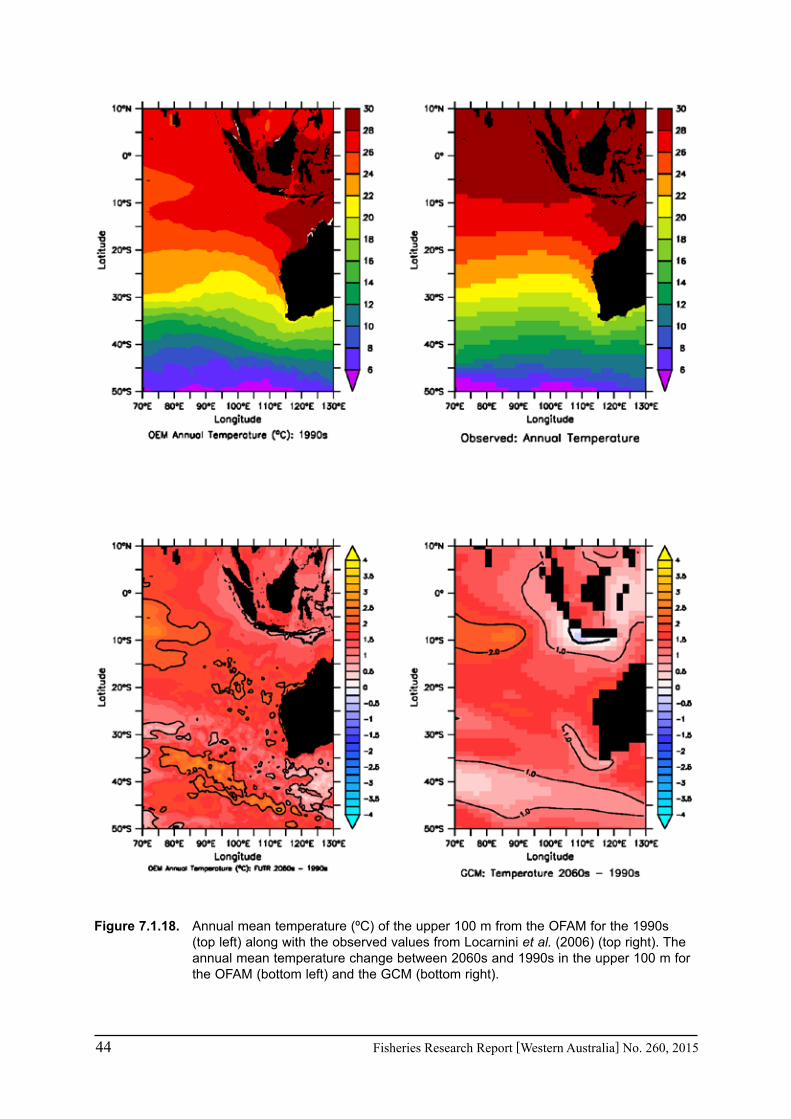
44 Fisheries Research Report [Western Australia] No. 260, 2015
Figure 7.1.18. Annual mean temperature (ºC) of the upper 100 m from the OFAM for the 1990s (top left) along with the observed values from Locarnini et al. (2006) (top right). The annual mean temperature change between 2060s and 1990s in the upper 100 m for the OFAM (bottom left) and the GCM (bottom right).
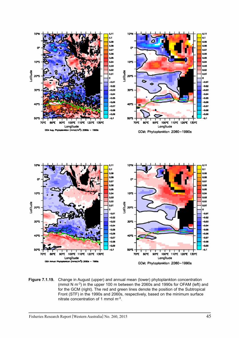
Fisheries Research Report [Western Australia] No. 260, 2015 45
Figure 7.1.19. Change in August (upper) and annual mean (lower) phytoplankton concentration (mmol N m-3) in the upper 100 m between the 2060s and 1990s for OFAM (left) and for the GCM (right). The red and green lines denote the position of the Subtropical Front (STF) in the 1990s and 2060s, respectively, based on the minimum surface nitrate concentration of 1 mmol m-3.

46 Fisheries Research Report [Western Australia] No. 260, 2015
Figure 7.1.20. Seasonal evolution of phytoplankton and zooplankton concentrations in the subtropics averaged over 0–100m at 32–33°S, 120–100°E (left) and 28–29°S, 10–100°E (right).

Fisheries Research Report [Western Australia] No. 260, 2015 47
Figure 7.1.21. Eddy kinetic energy (m2s-2) derived from the sea-surface height anomaly for the OFAM in 1990s (top left); for the observations (top right); for the change in the OFAM eddy kinetic energy between the 2060s – 1990s (bottom left).
Sea surface temperature
From the 1990s to the 2060s, the seasonally-averaged sea surface temperature (SST) increases for all seasons (Figure 7.1.22). The OFAM and ROMS 2060s solutions show a similar SST pattern, although the SST in ROMS 2060s tends to be cooler near the coast. From Figure 7.1.23 and Table 7.1.2, the mean SST over the entire shelf (from the coast (30 m) to 100 m isobath)

48 Fisheries Research Report [Western Australia] No. 260, 2015
increases by at least 1.8°C (in autumn) to 2.2°C (in winter). The warming over the shelf is similar to warming offshore for all seasons. Both the shelf and offshore regions tend to warm fastest in winter in the southern part of the domain (28.0°S to 34.6°S). The range of increased SST over the 70-year period yields warming rates ranging from 0.026°C/year to 0.033°C/year, which are consistent with observed warming rates over a 1985-2004 time period near 32°S but are greater than the observed warming rate of ~0.02°C/year over 50-years from global temperature datasets (Pearce and Feng 2007).
Coastal meridional transport
To assess changes in the coastal alongshore transport, the meridional flow is depth-integrated and integrated from the coast to the offshore limit of the current (Figure 7.1.24). The offshore limit is dynamically determined from the model result: In order to compare changes in the alongshore transport over the shelf, the coastal meridional transport is calculated as the maximum northward transport shorewards of h = 100 m depth at each latitude. If only southward transport is present, the coastal meridional transport is the accumulated transport at the first grid point offshore of h = 100 m.
The accumulated meridional transport is maximum northwards in summer when there are the strongest equatorward winds, and the Leeuwin Current then being weakest and the Capes Current strongest (Figure 6.1.3). The meridional transport shows regions of northward transport in spring but is predominantly southward in autumn and winter, when the equatorward winds are weakest or change direction. The ROMS solutions tend to be negatively biased from the OFAM solutions, with weaker northward transport in summer.
The OFAM solutions show that the mean meridional transport tends to decrease in all seasons despite local regions of increase (Figure 7.1.25). More southward meridional coastal transport is found in the southern part of the domain, possibly due to the onshore invasion of the Leeuwin Current (Table 7.1.3). From OFAM, the northward transport decreases in summer despite an increase in equatorward winds (Figure 6.1.3). The coastal meridional transport from ROMS is weaker than from OFAM although the transport from ROMS shows a similar peak in northward transport at 29.5°S in summer. The Hovmöller diagram of coastal meridional transport (Figure 7.1.26) reveals that the northward Capes Current (>0.05 Sv) occurs between November and March in OFAM 1990s and OFAM 2060s and between mid-November and mid-February in ROMS 2060s. All model solutions show that the strongest northward flow (>0.1 Sv) tends to occur south of 28°S.
Several key areas are examined in more detail, including Exmouth Gulf, Shark Bay, and the Capes Current. The temperature and velocity fields are examined in summer and time-averaged from December through February.
Exmouth Gulf and Shark Bay: temperature and circulation
The near-surface velocity field (Figure 7.1.27) and SST (Figure 7.1.28) show notable differences between the OFAM and ROMS projections. OFAM poorly resolves Exmouth Gulf and the velocity fields indicate offshore flow rather than an equatorward Ningaloo Current. ROMS also does not capture an equatorward Ningaloo Current and the circulation within Exmouth Gulf shows an inflow in the upper 10 m. From the 1990s to 2060s, the SST within Exmouth Gulf in OFAM locally increases but ROMS, with higher resolution, does not show as significant an increase. In the 2060s, ROMS tends to show cooler water adjacent to the offshore side of the coast and its difference with OFAM may reflect locally enhanced upwelling given higher resolution.
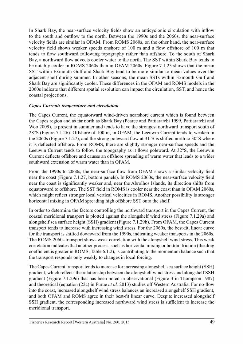
Fisheries Research Report [Western Australia] No. 260, 2015 49
In Shark Bay, the near-surface velocity fields show an anticyclonic circulation with inflow to the south and outflow to the north. Between the 1990s and the 2060s, the near-surface velocity fields are similar in OFAM. From ROMS 2060s, on the other hand, the near-surface velocity field shows weaker speeds onshore of 100 m and a flow offshore of 100 m that tends to flow southward following topography rather than offshore. To the south of Shark Bay, a northward flow advects cooler water to the north. The SST within Shark Bay tends to be notably cooler in ROMS 2060s than in OFAM 2060s. Figure 7.1.23 shows that the mean SST within Exmouth Gulf and Shark Bay tend to be more similar to mean values over the adjacent shelf during summer. In other seasons, the mean SSTs within Exmouth Gulf and Shark Bay are significantly cooler. These differences in the OFAM and ROMS models in the 2060s indicate that different spatial resolution can impact the circulation, SST, and hence the coastal projections.
Capes Current: temperature and circulation
The Capes Current, the equatorward wind-driven nearshore current which is found between the Capes region and as far north as Shark Bay (Pearce and Pattiaratchi 1999, Pattiaratchi and Woo 2009), is present in summer and tends to have the strongest northward transport south of 28°S (Figure 7.1.26). Offshore of 100 m, in OFAM, the Leeuwin Current tends to weaken in the 2060s (Figure 7.1.27), and the strong poleward flow at 31°S is shifted north to 30°S where it is deflected offshore. From ROMS, there are slightly stronger near-surface speeds and the Leeuwin Current tends to follow the topography as it flows poleward. At 32°S, the Leeuwin Current deflects offshore and causes an offshore spreading of warm water that leads to a wider southward extension of warm water than in OFAM.
From the 1990s to 2060s, the near-surface flow from OFAM shows a similar velocity field near the coast (Figure 7.1.27, bottom panels). In ROMS 2060s, the near-surface velocity field near the coast is significantly weaker and, near the Abrolhos Islands, its direction shifts from equatorward to offshore. The SST field in ROMS is cooler near the coast than in OFAM 2060s, which might reflect stronger local vertical velocities in ROMS. Another possibility is stronger horizontal mixing in OFAM spreading high offshore SST onto the shelf.
In order to determine the factors controlling the northward transport in the Capes Current, the coastal meridional transport is plotted against the alongshelf wind stress (Figure 7.1.29a) and alongshelf sea surface height (SSH) gradient (Figure 7.1.29b). From OFAM, the Capes Current transport tends to increase with increasing wind stress. For the 2060s, the best-fit, linear curve for the transport is shifted downward from the 1990s, indicating weaker transports in the 2060s. The ROMS 2060s transport shows weak correlation with the alongshelf wind stress. This weak correlation indicates that another process, such as horizontal mixing or bottom friction (the drag coefficient is greater in ROMS; Table 6.1.2), is contributing to the momentum balance such that the transport responds only weakly to changes in local forcing.
The Capes Current transport tends to increase for increasing alongshelf sea surface height (SSH) gradient, which reflects the relationship between the alongshelf wind stress and alongshelf SSH gradient (Figure 7.1.29c) that has been noted in observational (Figure 3 in Thompson 1987) and theoretical (equation (22c) in Furue et al. 2013) studies off Western Australia. For no-flow into the coast, increased alongshelf wind stress balances an increased alongshelf SSH gradient, and both OFAM and ROMS agree in their best-fit linear curve. Despite increased alongshelf SSH gradient, the corresponding increased northward wind stress is sufficient to increase the meridional transport.

50 Fisheries Research Report [Western Australia] No. 260, 2015
The depth-integrated y-momentum equation shows the competing local forcing terms:
∂V/∂t + f U = - g h ∂(SSH)/∂y + ( τy/ρo ) - cD |v (z = -h) | v (z = -h), (1)
where U and V are depth-integrated velocity components in the zonal and meridional direction, respectively, g is gravitational acceleration, h is the depth of the water column, τy is the meridional wind stress, ρo is the mean density, and cD is the quadratic bottom drag coefficient. With increasing water depth h, the alongshelf pressure gradient term (first term on the right side of (1)) dominates over the northward wind stress term (second term on the right side of (1)) and drives a poleward flow. Near the coast, the water depth is shallower and the northward wind stress dominates. Following Thompson (1987), the depth where the two forces are of equal and opposite contributions predicts where the meridional flow reverses sign, i.e. at
hCapes Current = ( τy/ρo ) / (g ∂(SSH)∂y). (2)
This represents the offshore limiting depth of the Capes Current, with poleward flow offshore of hCapes Current and equatorward flow inshore of this depth. From the models, this depth is estimated from the depth, hmax, where a maximum northward transport occurs over the shelf. Offshore of hmax, southward flow reduces the accumulated northward transport. Figure 7.1.29d shows the correlation between hmax and the predicted hCapes Current. In OFAM, hmax tends to be deeper, ~40 - 100 m, than in ROMS, ~30 - 60 m. The slopes of the best-fit linear curves indicate that the offshore limiting depth of the Capes Current increases for increasing wind stress and decreasing alongshelf SSH gradient (Table 7.1.4). However, this depth’s scaling with the forcing terms has a weaker dependence than predicted. This force balance has consequences for the cross-shelf circulation, including upwelling patterns.
Two cross-sections are presented for the mean summer fields. One section is at 29.5°S, where both OFAM and ROMS models have a maximum northward transport in summer, and another section is at 34.0°S, which has been a focus of past Capes Current studies (e.g. Pearce and Pattiaratchi 1999; Gersbach et al. 1999).
At 29.5°S (Figure 7.1.30), the shelf warms significantly from the 1990s to 2060s, with warming occurring at depths below 200 m and the 20.0°C isotherm shifting down 50 m. In ROMS 2060s, there is cooler water over the shelf, and offshore the warming is more surface-trapped. At this latitude, the poleward flow is not significantly weaker in the 2060s than in the 1990s. The Leeuwin Current has an eastward component as it flows poleward along the continental slope. The northward wind stress leads to an offshore surface Ekman flow that is over a thinner depth in ROMS, ~10 m, than OFAM, ~20 m, and may be due to the stronger stratification near the surface in ROMS. Near the coast the northward flow is ~ 0.2 m/s, and is over a deeper depth in OFAM, ~70 m, than ROMS, ~50 m. Both models show two upwelling cells, with wind-driven upwelling right at the coast and upwelling at the shelf break which may be due to a convergence in the bottom Ekman flow (e.g. Thompson 1987). On the shelf, these upwelling cells are closed, with downwelling near where the meridional flow reverses direction.
At 34.0°S, the mean summer velocity and temperature fields show similar features although the shelf is narrower (Figure 7.1.31). The Leeuwin Current tends to weaken from the 1990s to the 2060s and the temperature increases with the 20.0°C isotherm shifting downward by 30 to 50 m. There is offshore, eastward flow that partly converges and downwells within the Leeuwin Current, and a westward, surface Ekman flow that is over a thinner depth in ROMS due to greater stratification. The two-upwelling cells are also present at this section. The offshore upwelling may be greater at this latitude due to stronger Leeuwin Current speeds near the bottom inducing stronger offshore bottom Ekman flows. Furthermore, the greater drag coefficient in ROMS

Fisheries Research Report [Western Australia] No. 260, 2015 51
than OFAM (Table 6.1.2) may contribute to stronger bottom Ekman transports. Hence this may contribute to the stronger upwelling offshore of the shelf break in ROMS than OFAM.
In order to link upwelling with the alongshelf wind stress and flow field, the daily-mean vertical velocity in ROMS 2060 is calculated during the summer months. The cross-shelf sections at 29.5°S and 34.0°S indicate that there are two maxima in the vertical velocity, one near the coast and another near the shelf break. From each section, the maximum vertical velocities were determined within an offshore range from 200 m < h < 50 m or near the coast from 50 m < h < 30 m (at the coast). The vertical velocity is compared with the alongshelf wind stress (Figure 7.1.32a,b) and the local near-bottom meridional velocity (Figure 7.1.32c,d). The near-bottom meridional velocity is used for comparison since the bottom Ekman transport is proportional to the near-bottom flow speed. Offshore, the maximum vertical velocity does not show a clear dependence on the alongshelf wind stress or near-bottom meridional flow (Table 7.1.5). The maximum vertical velocity is present for either northward or southward flow and tends to have greater values than near the coast. Near the coast, the vertical velocity tends to increase for increasing wind stress at both sections. The vertical velocity shows a stronger dependence on the alongshelf wind stress and near-bottom velocity at 34.0°S than at 29.5°S.
Table 7.1.2. Mean change in SST (°C) from OFAM over the shelf and offshore region for 1990s to 2060s.
Season Entire domain (21.0°S to 35.0°S)shelf, offshore SST (°C)
Southern part of domain (28.0°S to 34.6°S)shelf, offshore SST (°C)
Summer 1.9, 1.8 1.8, 1.8
Autumn 1.8, 1.8 1.9, 1.9
Winter 2.2, 2.1 2.2, 2.3
Spring 2.0, 1.9 1.8, 1.8
Table 7.1.3. Mean coastal meridional transport (Sv) from 28.0°S to 34.0°S. 1 Sv = 106 m3s-1
Season OFAM 1990s Transport (Sv)
OFAM 2060s Transport (Sv)
ROMS 2060s Transport (Sv)
Summer 0.13 0.12 0.07
Autumn -0.10 -0.12 -0.20
Winter -0.38 -0.40 -0.34
Spring 0.02 -0.004 -0.11
Table 7.1.4. Best-fit, linear curves, where τa is the alongshelf wind stress, and dSSH/dya is the alongshelf sea surface height (SSH) gradient.
OFAM 1990s OFAM 2060s ROMS 2060s
(a) Transport (Sv) 1.0 x τa/(N m-2) 1.2 x τa/(N m-2) 0.1 x τa/(N m-2) + 0.1
(b) Transport (Sv) 2.4 x 10⁵ x (dSSH/dya) + 0.1 4.2 x 10⁵ x (dSSH/dya) 0.5 x 10⁵ x (dSSH/dya)
+ 0.1
(c) Alongshelf SSH gradient x 10-7 14.8 x τa/(N m-2) + 0.4 17.3 x τa/(N m-2) + 0.2 17.6 x τa/(N m-2) + 0.1
(d) hmax (m) 0.3 x ((τa/ρo)/(g x dSSH/dya)) + 44.4
0.1 x ((τa/ρo)/(g x dSSH/dya)) + 56.7
0.4 x ((τa/ρo)/(g x dSSH/dya)) + 30.4

52 Fisheries Research Report [Western Australia] No. 260, 2015
Table 7.1.5. Best-fit, linear curves, where τa is the alongshelf wind stress, and vbottom is the near bottom meridional velocity.
29.5oS 34.0oS
(c) Coastal maximum vertical velocity (m/day) 15.4 x τa/(N m-2) + 9.9 61.9 x τa/(N m-2) + 7.0
(b) Coastal maximum vertical velocity (m/day) 0.1 x vbottom/(m s-1) + 11.2 46.1 x vbottom/(m s-1) + 12.7
Figure 7.1.22. The seasonally-averaged sea surface temperature (°C) in summer (months DJF), autumn (MAM), winter (JJA), and spring (SON) from OFAM and ROMS for 1990s and 2060s. The thick black lines are the 20°C, 25°C, and 30°C isotherms. The 100 m isobath (pink line) is also shown.

Fisheries Research Report [Western Australia] No. 260, 2015 53
Figure 7.1.23. Top panels. The seasonally-averaged sea surface temperature (SST, °C) with latitude. The mean shelf SST is calculated from h = 100 m to the coast, where ROMS excludes the Exmouth Gulf and Shark Bay regions enclosed by the 40 m isobath (see Figure 6.1.2). The mean offshore SST is calculated from 1° longitude offshore of 100 m isobath. The mean SST is calculated from OFAM 1990s (shelf: black line; offshore: grey line), OFAM 2060s (shelf: blue line; offshore: light blue), and ROMS 2060s (shelf: red line). From ROMS 2060s, the mean SST is calculated for values within Exmouth Gulf (Δ) and Shark Bay (*) and for values surrounding the Abrolhos Islands (o). Bottom panels. The change in the SST (2060s – 1990s) from OFAM over the shelf (blue line) and offshore region (black line).

54 Fisheries Research Report [Western Australia] No. 260, 2015
Figure 7.1.24. The seasonally-averaged, accumulated meridional transport (Sv) integrated offshore from the coast. The thick black line indicates the coastal position used in calculating the transport, which excludes Exmouth Gulf and Shark Bay in both models.

Fisheries Research Report [Western Australia] No. 260, 2015 55
Figure 7.1.25. Top panels. The coastal meridional transport (Sv) for each season. The coastal meridional transport is the maximum equatorward transport from the coast out to the first point offshore of h = 100 m. If no equatorward flow is present, then the coastal transport is the value immediately offshore of h = 100 m. The coastal transport is calculated from OFAM 1990s (black line), OFAM 2060s (blue line), and ROMS 2060 (red line). The mean coastal meridional transport for each season is given by the values in Table 7.1.3. Bottom panels. The change in the coastal meridional transport (2060s – 1990s) from OFAM.
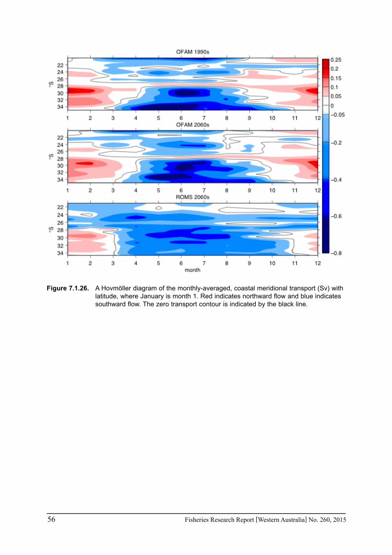
56 Fisheries Research Report [Western Australia] No. 260, 2015
Figure 7.1.26. A Hovmöller diagram of the monthly-averaged, coastal meridional transport (Sv) with latitude, where January is month 1. Red indicates northward flow and blue indicates southward flow. The zero transport contour is indicated by the black line.

Fisheries Research Report [Western Australia] No. 260, 2015 57
Figure 7.1.27. The summer velocity field, averaged over the top 10 m, where speed is colour-coded (m/s) according to the scale on the right and the arrows indicate the velocity direction. The top panels show Exmouth Gulf, the middle panels show Shark Bay, and the bottom panels show the southern part of the shelf, including the Capes Current. The 100 m isobath is indicated by the pink line and the coastline by the thick black line.
Figure 7.1.28. The summer sea surface temperature (°C), where the arrows indicate the near-surface velocity direction, and the panels correspond to the regions in Figure 7.1.27.
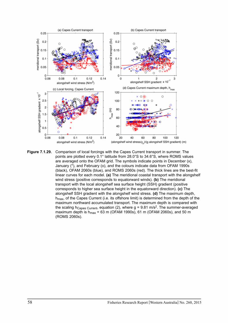
58 Fisheries Research Report [Western Australia] No. 260, 2015
Figure 7.1.29. Comparison of local forcings with the Capes Current transport in summer. The points are plotted every 0.1° latitude from 28.0°S to 34.6°S, where ROMS values are averaged onto the OFAM grid. The symbols indicate points in December (x), January (*), and February (o), and the colours indicate data from OFAM 1990s (black), OFAM 2060s (blue), and ROMS 2060s (red). The thick lines are the best-fit linear curves for each model. (a) The meridional coastal transport with the alongshelf wind stress (positive corresponds to equatorward winds). (b) The meridional transport with the local alongshelf sea surface height (SSH) gradient (positive corresponds to higher sea surface height in the equatorward direction). (c) The alongshelf SSH gradient with the alongshelf wind stress. (d) The maximum depth, hmax, of the Capes Current (i.e. its offshore limit) is determined from the depth of the maximum northward accumulated transport. The maximum depth is compared with the scaling hCapes Current, equation (2), where g = 9.81 m/s2. The summer-averaged maximum depth is hmax = 63 m (OFAM 1990s), 61 m (OFAM 2060s), and 50 m (ROMS 2060s).

Fisheries Research Report [Western Australia] No. 260, 2015 59
Figure 7.1.30. Summer (DJF) average of the u (eastward, m/s), v (northward, m/s), and w (vertical, m/day) current velocity components coded by the colour bars on the right, and the temperature field (black contours) at 29.5°S. The temperature is plotted every 1.0°C, the thick contours showing the 20.0°C and 25.0°C isotherms. The velocity field’s zero speed is given by the white line.
Figure 7.1.31. Same as Figure 7.1.30 for 34.0°S.

60 Fisheries Research Report [Western Australia] No. 260, 2015
Figure 7.1.32. Upwelling in summer from ROMS 2060s. The daily-mean, maximum vertical velocity is compared with the daily-mean alongshelf wind stress (top panels) and the local near-bottom meridional velocity (bottom panels). The maximum vertical velocity is calculated between 200 m < h < 50 m (offshore; left panels) and 50 m < h < coast (coastal; right panels). The vertical velocities are plotted at 29.5°S (blue points) and 34.0°S (red points) for December (x), January (*), and February (o). The summer-averaged maximum vertical velocities are 18 m/day offshore and 11 m/day near the coast at 29.5°S and 20 m/day offshore and 14 m/day near the coast at 34.0°S. The lines in (b,d) are the linear best-fit curves.
Shelf-scale changes from the Northwest shelf to the south coast
From the 1990s to the 2060s, OFAM shows warming sea surface temperatures in all seasons from the Northwest shelf to the south coast of Western Australia (Figure 7.1.33). The warming “hot spots”, where temperature rises over that interval exceed 2.5°C, tend to occur off the west coast (22.5°S to 34.35°S) rather than the Northwest shelf (north of 22.5°S) or the south coast (east of 115.15°E). The greatest regional increase in SST occurs offshore from the coast in winter, while the mean coastal SST rise inshore of the 200 m isobath is greatest in winter and spring on the Northwest shelf and off the west coast in winter (Figure 7.1.34, Figure 7.1.35, Table 7.1.6). The change in coastal SST off the south coast does not show as significant warming as the other regions.
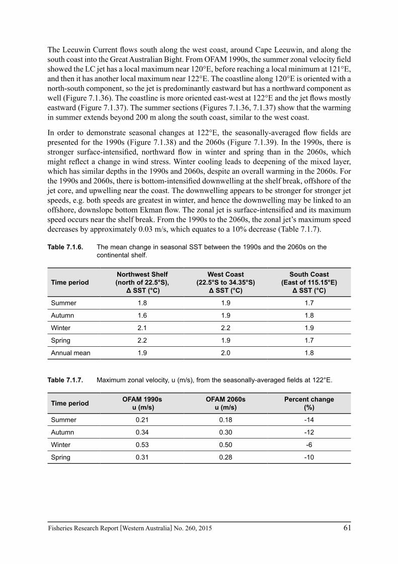
Fisheries Research Report [Western Australia] No. 260, 2015 61
The Leeuwin Current flows south along the west coast, around Cape Leeuwin, and along the south coast into the Great Australian Bight. From OFAM 1990s, the summer zonal velocity field showed the LC jet has a local maximum near 120°E, before reaching a local minimum at 121°E, and then it has another local maximum near 122°E. The coastline along 120°E is oriented with a north-south component, so the jet is predominantly eastward but has a northward component as well (Figure 7.1.36). The coastline is more oriented east-west at 122°E and the jet flows mostly eastward (Figure 7.1.37). The summer sections (Figures 7.1.36, 7.1.37) show that the warming in summer extends beyond 200 m along the south coast, similar to the west coast.
In order to demonstrate seasonal changes at 122°E, the seasonally-averaged flow fields are presented for the 1990s (Figure 7.1.38) and the 2060s (Figure 7.1.39). In the 1990s, there is stronger surface-intensified, northward flow in winter and spring than in the 2060s, which might reflect a change in wind stress. Winter cooling leads to deepening of the mixed layer, which has similar depths in the 1990s and 2060s, despite an overall warming in the 2060s. For the 1990s and 2060s, there is bottom-intensified downwelling at the shelf break, offshore of the jet core, and upwelling near the coast. The downwelling appears to be stronger for stronger jet speeds, e.g. both speeds are greatest in winter, and hence the downwelling may be linked to an offshore, downslope bottom Ekman flow. The zonal jet is surface-intensified and its maximum speed occurs near the shelf break. From the 1990s to the 2060s, the zonal jet’s maximum speed decreases by approximately 0.03 m/s, which equates to a 10% decrease (Table 7.1.7).
Table 7.1.6. The mean change in seasonal SST between the 1990s and the 2060s on the continental shelf.
Time periodNorthwest Shelf(north of 22.5°S),
Δ SST (°C)
West Coast(22.5°S to 34.35°S)
Δ SST (°C)
South Coast(East of 115.15°E)
Δ SST (°C)
Summer 1.8 1.9 1.7
Autumn 1.6 1.9 1.8
Winter 2.1 2.2 1.9
Spring 2.2 1.9 1.7
Annual mean 1.9 2.0 1.8
Table 7.1.7. Maximum zonal velocity, u (m/s), from the seasonally-averaged fields at 122°E.
Time period OFAM 1990s u (m/s)
OFAM 2060su (m/s)
Percent change(%)
Summer 0.21 0.18 -14
Autumn 0.34 0.30 -12
Winter 0.53 0.50 -6
Spring 0.31 0.28 -10
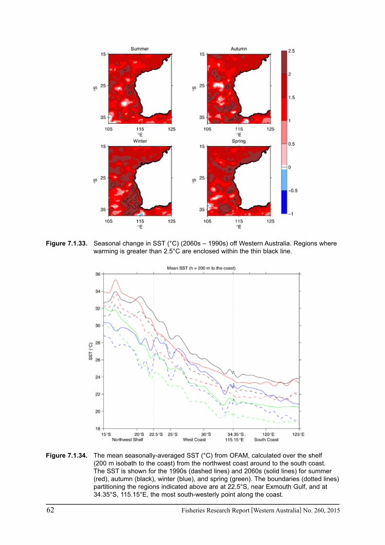
62 Fisheries Research Report [Western Australia] No. 260, 2015
Figure 7.1.33. Seasonal change in SST (°C) (2060s – 1990s) off Western Australia. Regions where warming is greater than 2.5°C are enclosed within the thin black line.
Figure 7.1.34. The mean seasonally-averaged SST (°C) from OFAM, calculated over the shelf (200 m isobath to the coast) from the northwest coast around to the south coast. The SST is shown for the 1990s (dashed lines) and 2060s (solid lines) for summer (red), autumn (black), winter (blue), and spring (green). The boundaries (dotted lines) partitioning the regions indicated above are at 22.5°S, near Exmouth Gulf, and at 34.35°S, 115.15°E, the most south-westerly point along the coast.

Fisheries Research Report [Western Australia] No. 260, 2015 63
Figure 7.1.35. The change in SST (°C) (2060s – 1990s) from OFAM, calculated over the shelf (200 m isobath to the coast). The change in SST is shown for summer (red), autumn (black), winter (blue), and spring (green).
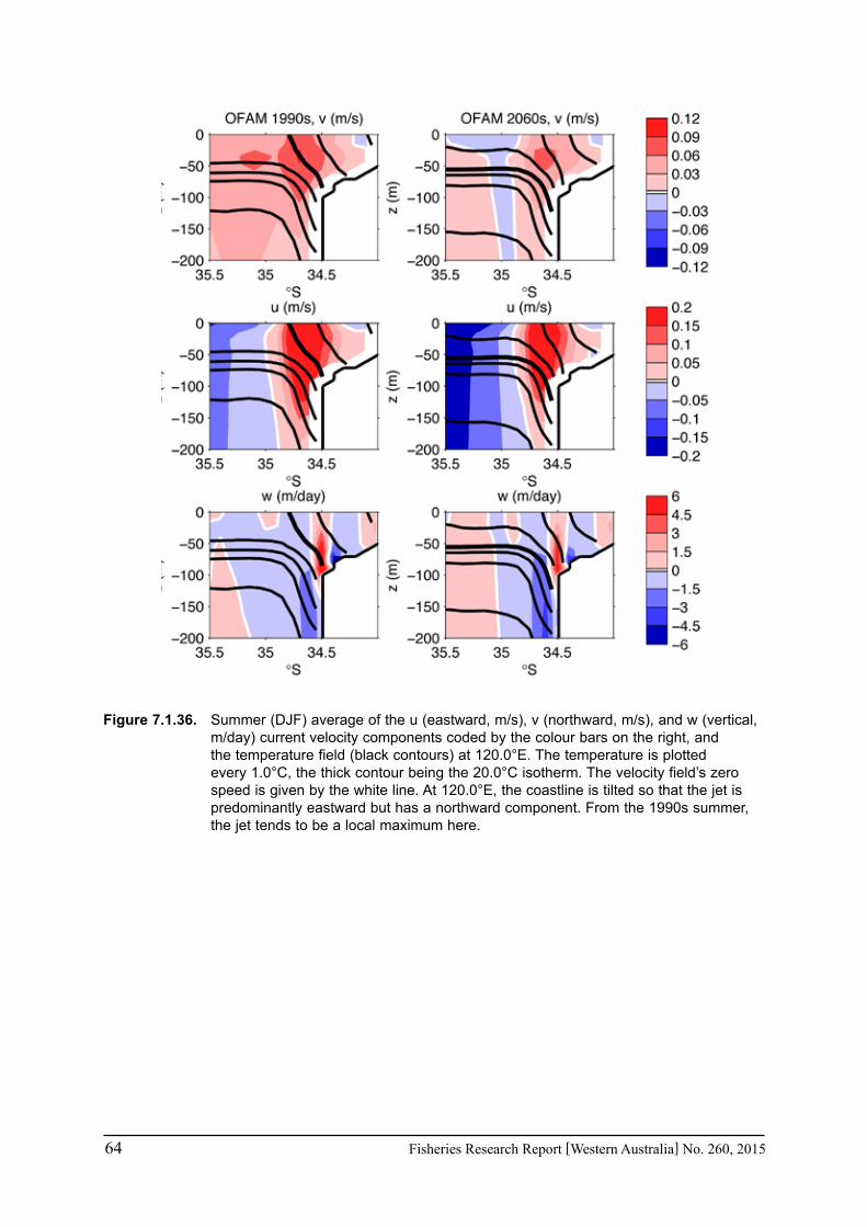
64 Fisheries Research Report [Western Australia] No. 260, 2015
Figure 7.1.36. Summer (DJF) average of the u (eastward, m/s), v (northward, m/s), and w (vertical,
m/day) current velocity components coded by the colour bars on the right, and the temperature field (black contours) at 120.0°E. The temperature is plotted every 1.0°C, the thick contour being the 20.0°C isotherm. The velocity field’s zero speed is given by the white line. At 120.0°E, the coastline is tilted so that the jet is predominantly eastward but has a northward component. From the 1990s summer, the jet tends to be a local maximum here.

Fisheries Research Report [Western Australia] No. 260, 2015 65
Figure 7.1.37. As for Figure 7.1.36 for 122.0°E.

66 Fisheries Research Report [Western Australia] No. 260, 2015
Figure 7.1.38. Seasonally-averaged fields at 122°E from 1990s OFAM. The seasons are shown from left to right panels: Summer (DJF months), Autumn (MAM), Winter (JJA), and Spring (SON). The flow field is shaded and shown for the meridional velocity (top panels), zonal velocity (middle panels), and vertical velocity (bottom panels). Temperature is contoured every 1.0°C, where the thick black line is 20°C and the thin grey line is 17°C for reference.
Figure 7.1.39. Seasonally-averaged fields at 122°E from 2060s OFAM.

Fisheries Research Report [Western Australia] No. 260, 2015 67
7.2 Effect of climate change on fish stocks
7.2.1 Case Studies
Seventeen case study species covering invertebrates and finfish from across key bioregional parts of the state and comprising a wide array of habitats were examined for climate change effects on key fisheries. The species include commercial invertebrate species such as Western Rock Lobster, Saucer Scallop, Blue Swimmer Crab, abalone (2 species), Octopus, Pearl Oyster, prawns (2 species), and key finfish species including Snapper, Australian Herring, Tailor, Australian Sardine (Pilchard), Narrow-Barred Spanish Mackerel, Bight Redfish and various Groper spp. (see Part 2)
Table 7.2.1.1 provides a summary of environmental effects on some of the biological characteristics of species and the long-term trend of the environmental variables. Water temperature was identified as the key environmental factor affecting many invertebrate species such as Western Rock Lobster, Pearl Oysters, scallops, Blue Swimmer Crabs and Western King Prawn. Water temperature has been shown to affect many aspects of the biology of these species such as spawning, larval phase, recruitment, growth, migration, and size at maturity (Table 7.2.1.1). The recruitment of some species was positively related to water temperature such as Western King Prawns in Shark Bay, Blue Swimmer Crabs in Cockburn Sound and Pearl Oysters near Broome. However others were negatively related to water temperature such as scallops in Shark Bay and the Abrolhos Is.
Water temperature was also shown to have a positive and negative effect at different stages of the life history for Western Rock Lobster and Blue Swimmer Crabs in Shark Bay (Table 7.2.1.1). Higher water temperature near February (influenced by the Leeuwin Current) during the early larval stages of the Western Rock Lobster has historically been identified as being positively related to the puerulus settlement in many studies (Pearce and Phillips 1988; Caputi et al. 2001). However water temperature increases in winter/spring at the onset of spawning has resulted in an earlier spawning time which appears to have had a negative effect on puerulus settlement (Section 7.2.4, Caputi et al. 2014c). The water temperature at the time of peak spawning of the crab stocks in Shark Bay during the winter has a positive relationship with recruitment. However the water temperature during the early juvenile phase in summer has a negative impact (Section 7.2.4).
These water temperature relationships for invertebrate stocks were generally based on reliable assessments with long-term data sets that have been peer-reviewed and therefore have a relatively high level of confidence (Table 7.2.1.2). These temperature effects are particularly important as the lower west coast of WA has been identified as one of the hotspots of water temperature increases in the Indian Ocean (Pearce and Feng 2007). While there are increases in water temperature over the last 50 years in the north-west and south coast of WA, they were not as large as in the lower west coast.
Water temperature variations off Western Australia are influenced by a long-term increasing trend (Pearce and Feng 2007), particularly in the autumn-winter period (Caputi et al. 2009), as well as an annual variation that is influenced by the strength of the Leeuwin Current. The Leeuwin Current has been shown to influence a number of fish stocks off the WA coast such as Western Rock Lobster, scallops, Western King Prawns as well as fish stocks such as Australian Herring and West Australian Salmon, Pilchards and Whitebait (Caputi et al. 1996; Lenanton et al. 2009b). The effect of the current on fish stocks may be due to a number of reasons e.g. its effect on water temperature, water movements affecting larval and juvenile distribution, and productivity associated with eddy structures.
68 Fisheries Research Report [Western Australia] No. 260, 2015
A reduction of the Leeuwin Current transport (strength) by 15–20% from the 1990s to 2060s is projected under the IPCC A1B scenario (Section 7.1.3). However the Leeuwin Current has experienced a strengthening trend during the past two decades, which has almost reversed the weakening trend experienced during the 1960s to early 1990s (Feng et al. 2011a). The climate models tend to underestimate the natural climate variability on decadal and multi-decadal time scales so that while the greenhouse gas forcing induced changes may be obvious in the long-time climate projection, e.g. 2100, for an assessment of short-term climate projection, e.g. 2030s, natural decadal climate variations still need to be taken into account. Hence there is uncertainty in the trend of the Leeuwin Current in the short-term and its potential effect on fisheries.
Cyclones off the north-west coast can have a significant effect on Banana and Tiger Prawns, and Pearl Oyster stocks as well as significantly affecting seagrass habitat. High summer rainfall that is associated with cyclonic activity has a positive effect on Banana Prawn recruitment in Nickol Bay, Onslow and the Kimberley in a similar fashion to its effect in the Northern Prawn Fishery (Vance et al. 1985; Staples et al. 1995). Cyclones have a negative effect on Pearl Oyster stocks during their larval phase which affects the abundance of 0+ recruitment which is measured as piggyback spat on culture-size oysters. Cyclones have had both a strongly positive and strongly negative effect on Tiger Prawn recruitment in Exmouth Gulf depending on the timing of the cyclone and its intensity (Penn and Caputi 1986). Cyclone Vance which traversed Exmouth Gulf in April 1999 had a positive effect on the recruitment that year but also significantly destroyed the seagrass nursery habitat which negatively affected recruitment in the following two years (Loneragan et al. 2013).
Winter storms that are generally associated with rainfall along the south-west coast were identified as positively affecting puerulus settlement in the early 1990s (Caputi and Brown 1993). The recent assessment of the cause of the low puerulus settlement has confirmed that winter storms continue to influence the level of settlement (Section 7.2.3, Caputi et al. 2014c). The rainfall associated with these storms also has an effect on stocks in the estuaries such as Blue Swimmer Crabs in Peel-Harvey by flushing the crabs to the marine environment where spawning takes place in the summer period. The long-term decline in winter storms and rainfall in this region could affect these fisheries (IOCI 2012).
Tailor and West Australian Dhufish recruitment is positively related to salinity levels, which is associated with strong northerly winds along the lower west coast during summer (Lenanton et al. 2009a). These environmental conditions probably reflect when the Capes Current is flowing strongly in a northward direction along the coast. The Capes Current generally flows inshore of the Leeuwin Current, particularly during the summer months.
The marine heat wave in the Gascoyne and mid-west region of WA during the summer of 2010/11 is an example of an extreme climate event that has had short-term and longer-term effects on fisheries. These effects on invertebrate and finfish stocks are examined in detail in Sections 7.2.4 and 7.2.5, respectively. A major immediate effect was the 99% mortality of Roei Abalone in the Kalbarri region. The abalone fishery in this region has been shut and research trials on the translocation of abalone from nearby unaffected areas into the depleted areas and the release of hatchery-reared abalone are being assessed. A longer-term effect has been the lack of recruitment of scallops in Shark Bay and the Abrolhos Is. and Blue Swimmer Crabs in Shark Bay. The adult populations of these stocks have also been severely affected. The fisheries for scallops and crabs in this area did not fully operate during 2012 and 2013. The annual pre-recruitment survey of scallops that has been undertaken in Shark Bay since 1982 has proved valuable for managers and the fishing industry in the early detection of this

Fisheries Research Report [Western Australia] No. 260, 2015 69
poor scallop recruitment year class and adult abundance so that management and commercial industry decisions were made to not fish in 2012. The abundance of Shark Bay crabs in the deep water region has also been monitored since 2000 and has been valuable in the detection of the downturn of this fishery and fishing ceased from April 2012.
An important outcome 24 months on from the 2010/11 marine heatwave has been the range extension of several prominent nearshore finfish species, whose resident breeding populations were previously found only as far south as the Gascoyne region. While individuals of each species have persisted in nearshore waters off the lower west coast over this period, range extensions may well be permanent for at least one of these species. Available evidence suggests that a viable breeding population of Rabbitfish, Siganus sp., has been established in the Cockburn Sound region near Perth where individuals of the species now regularly contribute to commercial and recreational catches. Monthly records of Fremantle Sea Level suggests the significantly earlier (January) onset of the strong Leeuwin Current during 2011 created the opportunity for larvae of this summer-breeding species from the Gascoyne to be transported south, and to settle in nearshore habitats off the lower west coast. It is postulated that elevated SST experienced during the two years since the marine heatwave have contributed to the survival of the newly settled juveniles.
These case studies have highlighted the value of measuring pre-recruit abundance of the key invertebrate fisheries in WA to monitor the year class recruitment strength (Caputi et al. 2014a). The pre-recruit year-class strength of some finfish stocks such as Tailor are also measured, however, for many key finfish stocks the year-class strength is obtained indirectly by ageing methods. Understanding year-class strength is not only valuable for stock assessment for these fisheries but is particularly valuable in detecting annual variation and long-term trends in recruitment and the environmental factors that are contributing to these trends. This becomes particularly important when assessing the long-term climate change effects of the environment on the recruitment of the key fisheries stocks.
Recommendations
The case studies highlighted a number of key gaps and recommendations for future research in the identification of climate change effects on fisheries (Table 7.2.1.3) which are discussed further in Section 9 (Further Developments). These can be classified into:
a. monitoring key environmental trends;
b. monitoring trends in key marine habitats such as seagrass, algae and the environmental factors affecting them;
c. downscaling of oceanographic modelling to coastal areas to assess climate change effects, particularly in the north-west and south coast of WA;
d. oceanographic research on the cause of the extreme heat wave event of summer of 2010/11 which continued into the following two summers and whether this is part of a long-term trend;
e. monitoring of fish stock recruitment and distribution (and other key biological parameters such as reproductive status) for the early detection of climate change effects; and
f. understanding effects of environmental variations on recruitment, distribution and other biological parameters of fish stocks.

70 Fisheries Research Report [Western Australia] No. 260, 2015
Table 7.2.1.1: Summary of environmental effects (positive or negative) on some of the biological characteristics of species and the long-term trend of the environmental variables (LC=Leeuwin Current)
Species Biological parameter
Environmental effect (time) on biological parameter
Historic trend environmental variable
Reference & comments
Western Rock Lobster
Puerulus
+ LC strength & SST (Feb - Mar)+ storms (rainfall Jul - Nov)
SST increasingRainfall decreasing
Pearce & Phillips 1988 Caputi & Brown 1993
Puerulus - Breeding time+ storms (rainfall May - Oct)
Rainfall decreasing FRDC 2009/018
Breeding time
+ bottom water temperature
Water temperature increasing FRDC 2009/018
Size at migration - SST (4 yr lag) SST increasing Caputi et al. 2010b
Size at maturity - SST (5 yr lag) SST increasing Melville-Smith &
de Lestang 2006
Pearl Oyster
0+ settlement
+ SST (summer)- rain (summer)
SST increasingRain increasing Hart et al. 2011
CPUE - wind northward (summer) (4 - 5 yr lag)
Wind northward decreasing Hart et al. 2011
Scallop Recruitment - LC Strength - SST
Variable LC SST increasing
Lenanton et al. 2009bCaputi et al. 1996
Banana Prawns Recruitment + Rainfall (Dec - Mar) Rainfall & cyclone
activity increasing Sporer et al. 2013
Tiger Prawns Recruitment +/- rainfall Increased cyclone
activityPenn and Caputi 1986Loneragan et al. 2013
King Prawns Recruitment + SST SST increasing Lenanton et al. 2009b
Blue Swimmer Crabs
Growth and reproduction + SST SST increasing de Lestang et al. 2003
RecruitmentShark Bay: + SST winter- SST summer
SST increasing Section 7.2.4
Recruitment Cockburn Sound:+ SST winter/spring SST increasing de Lestang et al. 2010
Spawning Peel-Harvey: rainfall affects flushing of crabs Rainfall decreasing Johnston et al. 2014
Tailor Recruitment + salinity Salinity increasing Lenanton et al. 2009aPearce and Feng 2007
West Australian Dhufish
Recruitment+ salinity+ wind northward (summer)
Wind northward increasing
Lenanton et al. 2009aPearce & Feng 2007
Whitebait + LC Variable LC Caputi et al. 1996Lenanton et al. 2009b
Snapper Spawning, growth SST increasing Jackson et al. 2010

Fisheries Research Report [Western Australia] No. 260, 2015 71
Table 7.2.1.2. Summary of key climate change effects of species that are currently occurring and predicted effects. The potential for range shift is indicated. The level of confidence on the statements (H=high, M=moderate, L=low).
Species Current climate change impacts Predicted climate change impacts
Western Rock Lobster
• Decline in puerulus settlement due to earlier breeding time and reduced winter storms (M).
• Earlier breeding time due to increasing winter temperature (H).
• Reduced size of migration and maturity due to increasing SST (H).
• Change in growth due to increase in SST and change in size of maturity (M)
• Changes in spatial distribution of abundance due to migration (M)
• Increase in catchability due to increase in SST (M)
• Weaker Leeuwin Current may affect abundance and distribution of puerulus (M)
Tiger Prawns
• Heat wave effect on seagrass habitat may have affected recruitment (L)
• Increased cyclone activity has positive and negative effect on recruitment depending on timing and intensity (H)
• Increased SST effect on recruitment (L)
King Prawns • Increased SST positive effect on recruitment
Banana Prawns
• Increased rainfall from cyclones has positive effect (M)
Scallops
• SST increase affects recruitment (M)• Marine heat wave effect on
recruitment (M)
• Increased SST has negative effect on recruitment (L-M)
• Weaker Leeuwin Current positive effect on abundance (L-M)
Blue Swimmer Crab
• Shark Bay: effect of heat wave (M)• Peel-Harvey: effect of decreased
rainfall on flushing of crabs (L)
• Shark Bay: Increased SST in winter has positive effect but increased SST in summer has negative effect (M)
• Cockburn Sound: increased SST winter has positive effect (H)
Pearl Oysters• Environmental changes in SST,
rainfall & northerly wind have positive & negative effects on recruitment
Octopus• Increased SST may result in fast
growth, earlier onset of maturity and reduced fecundity
Abalone Roei • SST increase affecting northern stocks • Continued decline in northern areas and increases south
Abalone Greenlip
• Reduced productivity west coast • Increased productivity south coast
Baldchin Groper
• Shift south in distribution from mid-west to metro area due to SST increase
Western Blue Groper
• Possible reduced abundance in south and west coast
• Change in distribution

72 Fisheries Research Report [Western Australia] No. 260, 2015
Snapper
• Shark Bay: Heat wave mortalities (H)• Oceanic stock: shift in centre of
distribution (M), change in timing of spawning, increased growth & stock productivity, LC effect on larval dispersal to south (L)
• South Coast: Increased spawning (M)
• Shift south in distribution (LM)• reduced spawning off Shark Bay• increased individual growth
Tailor • Increased abundance on south coast (M)
• Reduced spawning in north affecting recruitment south (M)
Australian Herring
• Increased SST, heat wave and stronger Leeuwin Current effect on shift south in distribution (M)
• Shift south in distribution (LM)• Reduced recruitment eastward if
Leeuwin Current weaker
Australian Sardine
• Reduced abundance on west coast (L) with niche taken by Scaly Mackerel (H)
• Change in distribution if Leeuwin Current weaker
Eightbar Grouper
• Range extension south-east but not reproductively active
• Shift south in spawning location• Shift eastward along south coast
Blue Spotted Emperor
• Range extension south • Change in abundance & distribution
Spanish Mackerel
• Range extension south• Reproductive period extended• Geographic range of spawning
extended
• Range extension south • Increased biomass
Red Emperor • May be resilient to changes
Bight Redfish • Dispersal influenced if Leeuwin Current weaker
Table 7.2.1.3. Summary of the key gaps in the knowledge of climate change effects on fish stocks and areas of future research required to address the gaps.
Species Key gaps Future research
General
• Long-term monitoring of key environmental variables
• Long-term monitoring of key habitat areas
• Oceanographic modeling downscaling in north-west and south coast of WA
• Cause and long-term trend of marine heat wave
Western Rock Lobster
• Effect of increasing SST on catchability.
• Effect of increasing SST on lobster habitat.
• Effect of changes in Leeuwin Current on puerulus settlement.
• Modeling growth changes
• Laboratory and field experiments•• Monitoring lobster habitat at key locations.•• Oceanographic larval model runs under
different Leeuwin Current scenarios.• Lobster tagging and ageing studies.
Tiger Prawns • Nursery habitat trends • Monitoring of seagrass habitat and effect of cyclones and SST
King Prawns • Effect of continued SST increases on recruitment
• Monitoring environmental and recruitment trends

Fisheries Research Report [Western Australia] No. 260, 2015 73
Banana Prawns
• Monitoring environmental and recruitment trends
Scallops • Cause of recruitment variation • Assess potential for restocking • Ageing of scallop and timing of recruitment
Blue Swimmer Crabs
• Cause of recruitment variation including recent heat wave
• Monitoring environmental and recruitment trends
Pearl Oysters• Environmental trends in SST,
rainfall & northerly wind and overall effect on recruitment
• Monitoring environmental and recruitment trends
Abalone• Effect of environment changes
e.g. SST increases on recruitment
• Monitoring environmental and recruitment trends
• Assess potential for restocking
Octopus • Environmental effects on recruitment
Baldchin & Western Blue Groper
• Effect of changes in SST and Leeuwin and Capes Current on distribution
• Monitoring environmental and recruitment trends
Pink Snapper
• Factors affecting recruitment variation
• inter-annual variation in spawning
• changes in growth/stock productivity
• increased predation (sharks)
• Monitoring environmental and recruitment trends
• Monitoring reproductive activity• Monitoring growth
Tailor• Tolerance of eggs/larvae
to changing environmental conditions
Australian Herring
• Factors affecting recruitment variation
• Spawning and recruitment dynamics
Bight Redfish
• Biology and stock structure• Effect of high SST in south coast
in 2013 • Effect of Leeuwin Current on
dispersal
• Research project underway
Pilchard• Tolerance of eggs/larvae
to changing environmental conditions
Eightbar Grouper
• Stock distribution changes • Determination of any reproductive range extension southward
Blue Spotted Emperor
• Biology and stock structure • Biological research project underway
Spanish Mackerel
• Confirmation of reproductive range extension southward
• Estimates of (spawning) biomass in all management zones
Red Emperor• Tolerance of eggs/larvae
to changing environmental conditions
• Assessing tolerance levels of eggs/larvae to changing environmental conditions

74 Fisheries Research Report [Western Australia] No. 260, 2015
7.2.2 Risk assessments
A risk screening of 35 of WA’s key commercial and recreational finfish (23) and invertebrate (12) species was undertaken, based on methods developed by the South-east Australian Climate Change group to assess the relative sensitivity of species to climate change (Pecl et al. 2011). This assessment identified Perth Herring, abalone species, Black Bream, Western Rock Lobster, Pink Snapper, Whiskery Shark, Tiger Prawn, Pearl Oyster, Bight Redfish, and Australian Herring, as the most sensitive to climate change (Table 7.2.2.1). These 10 species with the highest sensitivity covered the four marine bioregions of Western Australia (North Coast, Gascoyne, West and South Coast) as well as having crustacean, molluscs and finfish representation. The species identified as having the lowest sensitivity were Octopus, Eightbar Grouper, Spanish Mackerel and Red Emperor.
The sensitivity assessment of the four criteria of the abundance attribute showed that Whiskery Shark and abalone species were ranked the highest (Table 7.2.2.1). The sensitivity assessment for the distribution attribute resulted in abalone species, Black Bream and Perth Herring ranked the highest. The sensitivity assessment for phenology had Perth Herring, Tiger Prawns and Western Rock Lobster ranked the highest.
The environmental factors that contribute to the sensitivity of species to climate change can then be examined for any trends that may indicate the influence of climate change and hence provide an indication of the exposure (likelihood) of species to climate change. The historic environmental trends and expected effects of climate change for key environmental indicators predicted for 2060 for scenario A1B in the four bioregions of Western Australia highlight some important trends occurring that may affect fisheries (Table 7.2.2.2). Some key results from the assessment are:
• Water SST has increased over the last 40 years over all of WA, particularly in the Western Bioregion, and to a greater extent in the winter than the summer;
• SST are predicted to continue to increase at a higher rate (0.28-0.37oC per decade) with a slightly higher rate in winter;
• Salinity has shown some increase since the 1950s and these may also continue in the Western Bioregion to 2060 but it may decline in the other bioregions;
• The pH is estimated to have undergone a small decline in the last 100 years and may be expected to show some decline over the next 100 years (IPCC 2013);
• The northward wind stress in the Western Bioregion has strengthened in last 30 years and this trend is expected to continue;
• The eastward wind stress in the Southern Bioregion has weakened in last 30 years and this trend is expected to continue;
• The Leeuwin Current weakened from the 1950s to the early 1990s but has strengthened during the last two decades with the long-term projection indicating a weakening trend;
• The winter storms (measured by rainfall) affecting the Western and Southern Bioregions have generally weakened in the last 40 years and this is projected to continue;
• The summer rainfall that primarily affected the Northern and Gascoyne Bioregions and is influenced by tropical cyclones and the north-west cloud bands, has increased in last 40 years but this may be due to aerosol increase and predicted decrease assumes future reductions in aerosols (IOCI 2012);

Fisheries Research Report [Western Australia] No. 260, 2015 75
• The number and intensity of cyclones have remained steady historically, however they are projected to decrease in number but increase in intensity with a shift further south that is associated with increasing water temperatures (IOCI 2012).
These trends were then used in the assessment of exposure (likelihood) of species to climate change occurring based on historical and projected trends and the assessment of overall risk to climate change = sensitivity x exposure (Table 7.2.2.3). After taking into account the exposure, the assessment identified Perth Herring, Roe’s Abalone, Black Bream, Western Rock Lobster, Pink Snapper, Whiskery Shark, Tiger Prawns, scallops, Blue Swimmer Crabs and Australian Herring, as having the highest risk to climate change (Table 7.2.2.3).
The species with risk assessments were classified into their bioregion and asset classification (e.g. finfish broken down by estuarine, inshore demersal, nearshore, offshore demersal and pelagic) as undertaken in the DoF risk assessment approach (Table 7.2.2.4, Fletcher et al. 2010). This helped determine the climate change priorities for research/management by taking into account risk associated with climate change as well as the socio-economic importance of the fisheries in the bioregions.
After taking the socio-economic importance into the account the fisheries with the highest priorities were the inshore demersal finfish stocks on the west coast bioregion (Pink Snapper and Whiskery Sharks) followed by the Western Rock Lobster fishery. Other inshore demersal stocks (including Baldchin Groper, West Australian Dhufish, Thickskin Shark, Spangled Emperor) and nearshore finfish stocks in the west coast (including Australian Herring and Tailor) were also identified has having high priority. Invertebrate species (prawns, scallops and Blue Swimmer Crabs) in the Gascoyne region recorded the next highest priority.

76 Fisheries Research Report [Western Australia] No. 260, 2015
Table 7.2.2.1: Risk screening of WA’s commercial and recreational finfish and invertebrate species, based on criteria developed by the South-East Australian Climate Change group (Pecl et al. 2011), to determine species that were most sensitive to climate change.
Common Name SpeciesMean risk score
Abundance Distribution Phenology Total
Hig
h se
nsiti
vity
Perth Herring Nematalosa vlaminghi 1.75 2.75 2.75 7.25
Brownlip Abalone Haliotis conicopora 2 3 1.75 6.75
Black Bream Acanthopagrus butcherii 1.75 3 2 6.75
Greenlip Abalone Haliotis laevigata 1.75 3 1.75 6.5
Roe’s Abalone Haliotis roei 2 2.75 1.75 6.5
Tiger Prawn Penaeus esculentus 1.5 2.25 2.75 6.5
Western Rock Lobster Panulirus cygnus 1.75 1.75 2.75 6.25
Silver Lipped Pearl Oyster Pinctada maxima 1.75 2.25 2.25 6.25
Whiskery Shark Furgaleus macki 2.25 2.5 1.5 6.25
Pink Snapper Pagrus auratus 1.5 2 2.5 6.25
Med
ium
-hig
h se
nsiti
vity
Bight Redfish Centroberyx gerrardi 1.5 2.25 2.25 6
Australian Herring Arripis georgianus 1.75 1.75 2.5 6
Western Blue Groper Achoerodus gouldii 1.75 2.25 1.75 5.75
Southern Saucer Scallop Amusium balloti 1.5 2.25 2 5.75
King Prawn Penaeus latisulcatus 1.5 2 2.25 5.75
Blue Swimmer Crab Portunus armatus (pelagicus) 1.25 2 2.5 5.75
Mud Crab Scylla serrata & Scylla olivacea 1.25 2.25 2.25 5.75
Blue Threadfin Eleutheronema tetradactylum 1.5 2.5 1.75 5.75
Baldchin Groper Choerodon rubescens 1.75 2.25 1.75 5.75
Thickskin Carcharhinus plumbeus 2 1.5 2.25 5.75
WA Dhufish Glaucosoma hebraicum 1.75 2.25 1.75 5.75
Spangled Emperor Lethrinus nebulosus 1.75 2 2 5.75
King Threadfin Polydactylus macrochir 1.75 2.25 1.75 5.75
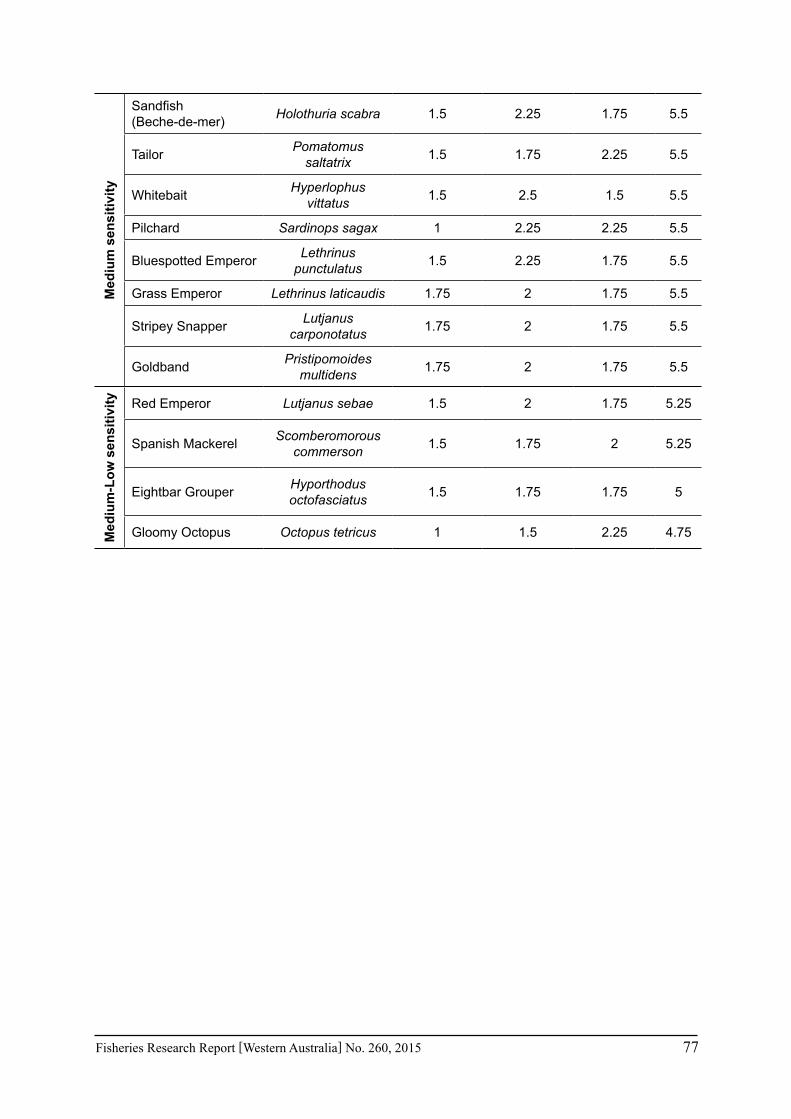
Fisheries Research Report [Western Australia] No. 260, 2015 77
Med
ium
sen
sitiv
itySandfish (Beche-de-mer) Holothuria scabra 1.5 2.25 1.75 5.5
Tailor Pomatomus saltatrix 1.5 1.75 2.25 5.5
Whitebait Hyperlophus vittatus 1.5 2.5 1.5 5.5
Pilchard Sardinops sagax 1 2.25 2.25 5.5
Bluespotted Emperor Lethrinus punctulatus 1.5 2.25 1.75 5.5
Grass Emperor Lethrinus laticaudis 1.75 2 1.75 5.5
Stripey Snapper Lutjanus carponotatus 1.75 2 1.75 5.5
Goldband Pristipomoides multidens 1.75 2 1.75 5.5
Med
ium
-Low
sen
sitiv
ity Red Emperor Lutjanus sebae 1.5 2 1.75 5.25
Spanish Mackerel Scomberomorous commerson 1.5 1.75 2 5.25
Eightbar Grouper Hyporthodus octofasciatus 1.5 1.75 1.75 5
Gloomy Octopus Octopus tetricus 1 1.5 2.25 4.75

78 Fisheries Research Report [Western Australia] No. 260, 2015
Table 7.2.2.2. (a) Historic climate changes for key environmental indicators in the four bioregions of Western Australia and (b) expected effects predicted for 2060 for the A1B scenario . Summarised from Section 7.1 and references indicated.
(a) Historic environmental changes
ENVIRONMENTALPARAMETER
MARINE BIOREGION YearReferenceNorth Gascoyne West South
SST winter oC per decadesummer oC per decade
<0.1 0.1
0.2 0.1
0.3 0.2
0.15<0.1
Caputi et al. 20091970-20121970-2012
Salinity psu0.0 0.1 0.1
0.00.1
Pearce & Feng 20071950-20001950-2012
pH -0.1 -0.1 -0.1 -0.1 1875-1995Northward wind stress Increase 1979-2012Eastward wind stress Decrease 1979-2012Leeuwin Current Weaker
No Change1950-19901950-2010
Tropical cyclones No trend numbers/ intensity
No trend numbers/ intensity
na naIOCI 201230 years
Rainfall winter na na Decrease Decrease IOCI 2012Rainfall summer Increase* Increase* na na IOCI 2012Primary productivity (ChlA)
No significant
change
Satellite remote sensing data since 1997
(b) Expected environmental changes (1990 to 2060)
ENVIRONMENTALPARAMETER
MARINE BIOREGION Reference
North Gascoyne West SouthSST winter oC per decadesummer oC per decade
0.35 0.3
0.35 0.3
0.37 0.32
0.320.28
Salinity psu Decrease Decrease Increase DecreasepH Decrease Decrease Decrease DecreaseNorthward wind stress IncreaseEastward wind stress DecreaseLeeuwin Current WeakerEastward jet WeakerTropical cyclones 50% less
but more intense
50% less but more intense.
100 km shift south
100 km shift southward
na IOCI 2012
Rainfall winter na na Decrease Decrease IOCI 2012Rainfall summer Decrease* Decrease* na na IOCI 2012Primary productivity (ChlA)
Increase No trend Decrease Decrease
*Current increase may be due to aerosol increase and predicted decrease assumes future reductions in aerosols (IOCI 2012).
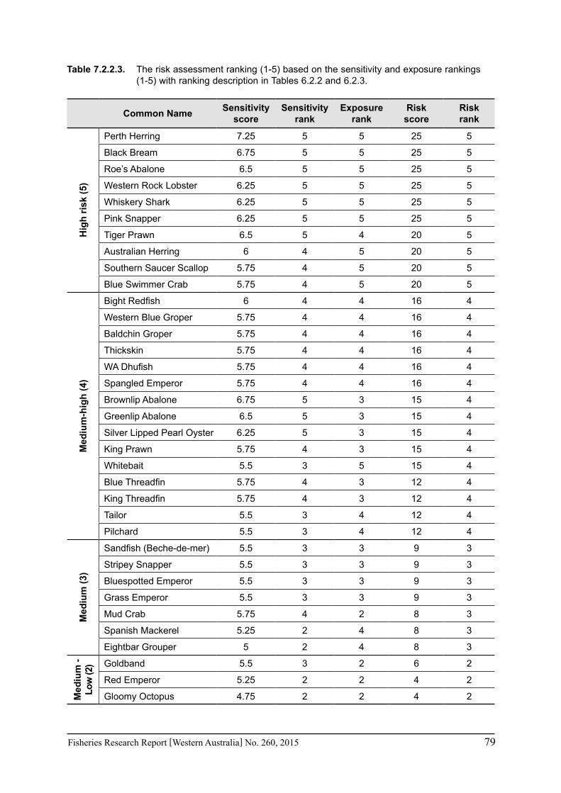
Fisheries Research Report [Western Australia] No. 260, 2015 79
Table 7.2.2.3. The risk assessment ranking (1-5) based on the sensitivity and exposure rankings (1-5) with ranking description in Tables 6.2.2 and 6.2.3.
Common Name Sensitivityscore
Sensitivityrank
Exposure rank
Risk score
Risk rank
Hig
h ris
k (5
)
Perth Herring 7.25 5 5 25 5
Black Bream 6.75 5 5 25 5
Roe’s Abalone 6.5 5 5 25 5
Western Rock Lobster 6.25 5 5 25 5
Whiskery Shark 6.25 5 5 25 5
Pink Snapper 6.25 5 5 25 5
Tiger Prawn 6.5 5 4 20 5
Australian Herring 6 4 5 20 5
Southern Saucer Scallop 5.75 4 5 20 5
Blue Swimmer Crab 5.75 4 5 20 5
Med
ium
-hig
h (4
)
Bight Redfish 6 4 4 16 4
Western Blue Groper 5.75 4 4 16 4
Baldchin Groper 5.75 4 4 16 4
Thickskin 5.75 4 4 16 4
WA Dhufish 5.75 4 4 16 4
Spangled Emperor 5.75 4 4 16 4
Brownlip Abalone 6.75 5 3 15 4
Greenlip Abalone 6.5 5 3 15 4
Silver Lipped Pearl Oyster 6.25 5 3 15 4
King Prawn 5.75 4 3 15 4
Whitebait 5.5 3 5 15 4
Blue Threadfin 5.75 4 3 12 4
King Threadfin 5.75 4 3 12 4
Tailor 5.5 3 4 12 4
Pilchard 5.5 3 4 12 4
Med
ium
(3)
Sandfish (Beche-de-mer) 5.5 3 3 9 3
Stripey Snapper 5.5 3 3 9 3
Bluespotted Emperor 5.5 3 3 9 3
Grass Emperor 5.5 3 3 9 3
Mud Crab 5.75 4 2 8 3
Spanish Mackerel 5.25 2 4 8 3
Eightbar Grouper 5 2 4 8 3
Med
ium
- Lo
w (2
) Goldband 5.5 3 2 6 2
Red Emperor 5.25 2 2 4 2
Gloomy Octopus 4.75 2 2 4 2

80 Fisheries Research Report [Western Australia] No. 260, 2015
Table 7.2.2.4. Combining species into bioregion and ecological assets using DoF risk assessment approach (Fletcher et al. 2010). Priority for research and management for climate change issues takes into account the socio-economic importance.
Bio-region Branch Ecological
suitesRisk assessment species
Risk level GVP Econ
riskSocial
amenitySocial
risk Priority
WC FF Inshore demersal
Whiskery Shark Pink Snapper 5 3 3 5 4 145
WC C Inshore Rock Lobster 5 5 3 4 3 135
WC FF Inshore demersal
Baldchin GroperThickskin Dhufish Spangled Emperor
4 3 3 5 4 116
WC FF NearshoreAust. HerringTailorWhitebait
5 1 3 5 4 115
G C Embayment Prawn sp.Scallop 5 5 4 1 1 105
G C Embayment Blue Swimmer Crab 5 5 5 2 3 105
NC FF Nearshore King ThreadfinBlue Threadfin 4 2 2 5 4 96
WC FF Estuarine Perth Herring Black Bream 5 1 3 4 4 95
WC M Nearshore Roe’s Abalone 5 3 3 4 2 85
SC M Nearshore Greenlip Abalone 4 4 3 2 1 56
NC M Inshore Pearl Oyster 4 5 2 3 1 52
SC FF Nearshore
Aust. HerringW. Blue GroperTailor Whitebait
5 2 2 3 2 50
NC FFOffshore demersal
GoldbandEmperors (4 sp)Eightbar Grouper
3 4 3 2 1 42
SC/WC FF Offshore
demersal Bight Redfish 4 2 2 2 1 28
SC FF Pelagic Pilchard 4 3 2 1 1 28
NC/GC/WC
FF Pelagic Spanish Mackerel 3 2 2 2 1 18
NC M Nearshore Sandfish 3 1 4 2 1 18
NC C Nearshore Mud Crab 3 1 1 1 1 6
WC M Inshore Gloomy Octopus 2 2 1 1 1 6
7.2.3 Western Rock Lobster major case study
The Western Rock Lobster fishery is one of the best fisheries in Australia to examine effects of climate change because of the availability of long time series of data to assess trends in the fishery (de Lestang et al. 2012) and its location in one of the hotspots of long-term increases in water temperature in the Indian Ocean (Pearce and Feng 2007). The fishery is influenced by a number of environmental factors such as water temperature, the strength of the Leeuwin Current, and the winter storms (Caputi et al. 2001). These key environmental factors can affect
Fisheries Research Report [Western Australia] No. 260, 2015 81
the Western Rock Lobster throughout its complex life cycle from spawning; the larval stages over the 9–11 months they spend offshore of the continental shelf (Pearce and Phillips 1988; Caputi and Brown 1993; Caputi et al. 2001); the level and spatial distribution of the puerulus settlement along the coast; the growth rates of the juveniles (Johnston et al. 2008); the size of the juveniles migrating from shallow (<40 m) to deeper water (40–100 m) and the subsequent catch distribution; the strength of their pre-adult northerly migration (de Lestang et al. 2011); their size at maturity (Melville-Smith and de Lestang 2006); the moulting of mature females from setose to non-setose condition (de Lestang and Melville-Smith 2006); and the catchability of lobsters in the pots (Morgan 1974). Caputi et al. (2010b) examined some climate change effects on biological parameters such as size at maturity and the size of migrating lobsters that were occurring as a result of increasing water temperatures. As there are many aspects of the life history of the Western Rock Lobster that are influenced by environmental effects, the sensitivity assessment of the stock resulted in the species being ranked as a high risk and therefore sensitive to climate change effects (Appendix 4 Western Rock Lobster).
More recently the decline in puerulus settlement in the last seven years has not been explained by factors such as the Leeuwin Current that were previously identified as affecting settlement variation (Pearce and Phillips 1986) and it appears that this decline may be due to long-term environmental factors. This long-term decline in lobster abundance has required researchers to assess the stock implications of these changes and the managers and industry to consider the management options for dealing with the decline. Therefore the fishery has been used as a major case study in this project of how the research, management and industry have responded to this possible climate change scenario.
Pearce and Phillips (1988) showed that puerulus settlement is much higher in La Niña years when the Leeuwin Current is flowing strongly and water temperatures are warmer during February-April than during El Niño events. Therefore changes in water temperature during February have historically been identified as having a significant effect on puerulus settlement (Caputi et al. 2001). However the settlements between 2007/08 and 2012/13 have been anomalously low suggesting that other factors dominated in these years. For example, a record-low settlement occurred in 2008/08 despite a strong Leeuwin Current that year. The breeding stock was generally within historic levels during this with very high breeding stock levels in most areas of the fishery since 2010/11.
An oceanographic larval model identified the timing of spawning as an important factor explaining some of the variation in puerulus settlement (Feng et al. 2011b, Caputi et al. 2014c). An examination of the timing for the start of spawning based on data from the fishery-independent breeding stock survey conducted since the early 1990s has indicated that in recent years there has been an earlier start to the spawning season. This earlier start appears to be due to higher water temperatures near the onset of spawning (October) since the mid-2000s. This may be a key factor why recent years have had consistently below-average settlement. It is possible that the earlier spawning causes a mismatch with other environmental factors affecting other life history stages such as peaks in ocean productivity, water currents that move the early stage larvae offshore, and/or storms that may assist the late stage larvae and puerulus return to the coast.
Rainfall during July to November was identified in the early 1990s as being a significant factor related to puerulus settlement (Caputi and Brown 1993; Caputi et al. 1995). In an update to this assessment, rainfall during May-October when combined with the breeding time index provided a good fit (R2=0.72) to the variation in puerulus settlement since the early 1990s (Caputi et al. 2014c). The rainfall represents an index of storm activity affecting water conditions in the

82 Fisheries Research Report [Western Australia] No. 260, 2015
lower west coast of Western Australia (WA) and is generally associated with westerly winds that may help bring larvae back to the coast. These two variables (breeding time and storms) provide a plausible hypothesis to explain the decline in puerulus settlement in recent years. This relationship also predicted a marked improvement in settlement for 2013/14 based on a later start to spawning in 2012 and above average rainfall in 2013. Preliminary indications are that the 2013/14 puerulus settlement will be well above average and the largest since 2000/01. Further verification with additional years is required to see whether this relationship is maintained.
There may be climate change implications associated with the environmental factors (water temperature and storm activity) affecting the spawning and larval period, respectively, as both these environmental variables are showing long-term trends. A strong increase in water temperature has been identified in the low west coast of WA (Pearce and Feng 2007), particularly in the autumn-winter (Caputi et al. 2009). This increase is projected to continue (Feng et al. 2012). The rainfall during May-October shows a declining trend since the early 1990s with four of the lowest values occurring in last seven years. This decline is part of a long-term trend of declining storm activity and rainfall in the south-west of WA that has intensified in the last 10 years (Indian Ocean Climate Initiative 2012). This decline has also been projected to continue.
The implications of the extended period of low settlement on the stock status and management of the fishery were examined using a spatial stock assessment model (de Lestang et al. 2012). An important component of the model and management of the fishery has been the use of the puerulus settlement to predict the recruitment to the fishery 3-4 years ahead (de Lestang et al. 2009). The potential effects on catch and egg production of continued fishing at the existing effort levels of 2007/08 and at significantly reduced levels (ca. 40-70%) were examined. The stock assessment modelling showed that continued fishing at 2007/08 levels would have resulted in the fishery achieving very low catch rates in 2011/12 and 2012/13 and the breeding stock falling below threshold biological reference levels by about 2012/13 (Caputi et al. 2014b). Hence proactive management measures were introduced in 2008/09 and 2009/10, resulting in nominal fishing effort reductions of 44 and 72%, respectively. These effort reductions were introduced in years when recruitment to the fishery was still good. They resulted in a significant increase in fishable biomass and very high catch rates during these two years as well as supporting the fishery during the following years with predicted low recruitment (to the fishery), which commenced in 2010/11 (Figure. 7.2.3.2, Reid et al. 2013). The fishery management was also changed from an input control to an output-control fishery using individual transferable quotas (ITQs) in 2010/11 with a conservative quota of 5500 t. which is well below the long-term average catch of 11,000 t.
As a result of these management measures, the spawning stock reached record levels in the 2011 and 2012 fishery-independent surveys. These reductions in catch and effort were associated with a significant reduction in the vessel numbers by 36% in 2009/10 compared to 2007/08 which has had socio-economic implications. The level of effort reductions implemented were also commensurate with the level of effort reductions estimated at about 50–70% of 2007/08 effort to produce maximum economic yield (MEY) to the fishery (Reid et al. 2013). The fishery profit was estimated to have increased by about $50 million per year since 2009/10 compared to that estimated if the 2007/08 high level of effort had continued.
This proactive management approach taking into account the predicted recruitment to the fishery can be contrasted with the more typical reactive management approach that occurs in response to declining catches in most fisheries. Without the puerulus-based catch and recruitment forecasts, the first sign of the recruitment failure would have been very low catches from “normal” fishing effort being applied to the poor year-classes. By then the stock abundance and commercial

Fisheries Research Report [Western Australia] No. 260, 2015 83
catch rates may have fallen to low, possibly uneconomic, levels and a significant reduction to the breeding stock would have resulted. The fishery provides an example of an appropriate adaptation management response to a long-term change in the abundance of the recruitment which has resulted in a reduction in catch and fishing effort which protects the spawning stock and ensures the long-term sustainability of the fishery. The MEY assessment under catch quota controls showed that an annual harvest rate of about 40% of legal biomass provides a socio-economic target reference level based on MEY (Caputi et al. 2014b). This target complements the existing threshold and limit reference points based on egg production that are associated with sustainability (Department of Fisheries 2013). The target harvest level based on the more-conservative MEY assessment was formally adopted by management and industry as part of the formal harvest strategy for the management of the fishery. Fishing at the target MEY level maintains the egg production well above the biological reference levels and therefore provides greater resilience to the stock under any adverse environmental perturbation such as that experienced with the 7 consecutive years of low settlement.
Caputi et al. (2010b) has previously identified that increasing water temperatures over 35 years may have resulted in a decrease in size at maturity and the size of migrating lobsters from shallow to deep water; an increase in abundance of undersize and legal-size lobsters in deep water relative to shallow water; and a shift in catch to deep water. The size of the migrating lobsters is related to the water temperature about the time of puerulus settlement (about 4 years previously). The water temperature increases also affect catchability, females moulting from setose to non-setose, timing of moults and timing of peak catch rates. These climate change effects have also been taken into account in the stock assessment model. Most fishery models generally assume that biological parameters do not change over the years (stationarity assumption) and they generally assume an average level of recruitment when making projections. These stationarity assumptions may become less robust under climate change scenarios. Long-term changes in the abundance of fish stocks, particularly declines, require an appropriate adjustment of fishing effort or catch quota, for the stocks to be managed sustainably.
Recommendations
The key recommendations for future research for this fishery include:
a. Monitoring of key environmental factors such as Leeuwin Current, SST and storms that have been identified as affecting biological parameters such as size at maturity, size at migration and puerulus settlement;
b. Assess the effect of environmental variability on onset of spawning and puerulus settlement to determine whether the recent seven years of below-average settlement is part of a long-term trend or whether the settlement will return to historic average levels;
c. Examine the oceanographic larval model to understand why the early spawning may be causing a mismatch with other environmental factors affecting other life history stages
d. Adjust stock assessment model and/or management settings to take into account the current and projected changes in biological characteristics that are affected by long-term environmental trends; and
e. Monitor the effects of fishing at the MEY level on the egg production and assess the importance of having increased resilience in stocks under climate change.

84 Fisheries Research Report [Western Australia] No. 260, 2015
Figure 7.2.3.1. Annual puerulus settlement of the Western Rock Lobster fishery at various locations throughout the fishery.
Figure 7.2.3.2. Catch, effort and catch rates in the Western Rock Lobster fishery highlighting the effect of catch and effort reductions in the last 4 years.

Fisheries Research Report [Western Australia] No. 260, 2015 85
7.2.4 Marine heat wave major case study: invertebrate fisheries
The marine heat wave of the summer of 2010/11 affected the marine communities over a large area of Western Australia, particularly the Gascoyne and mid-west region. The heat wave has been described as a unique Ningaloo Niño event due to the unusual alignment of intra-seasonal to inter-decadal processes, resulting in an unseasonable surge of the Leeuwin Current and the extreme warm condition in the austral summer of 2010/11 (Feng et al. 2013). The above-average summer temperatures continued in the following two summers, 2011/12 and 2012/13 with the latter summer resulting in record-high SST in Albany and Esperance on the South Coast and Ningaloo (see Section 7.1.2).
A workshop reviewing communities affected (Caputi et al. 2014d) highlighted fish kills at the time of the heat wave, range extension of many tropical fish species and a negative effect on recruitment of Australian Herring and Yellow-Eye Mullet (see Section 7.2.5), reduction in some temperate seaweed species (Wernberg et al. 2013), and coral bleaching (Depczynski et al. 2012). In particular it had a significant impact on a number of invertebrate fisheries in the Gascoyne (Shark Bay and Exmouth Gulf) and mid-west region including the Abrolhos Islands (Figure. 7.1.5). Several flood events in Shark Bay with both the Gascoyne and Wooramel Rivers flowing during the same period may have also added to the impacts.
The invertebrate fisheries affected included abalone in Kalbarri, scallops in Shark Bay and Abrolhos, Blue Swimmer Crabs in Shark Bay and Tiger and King Prawns in Shark Bay and Exmouth Gulf. This section examines the effect of water temperature, including the heat wave period, on key invertebrate fisheries. The heat wave represents an example of the effect of an extreme environmental event on fisheries and an opportunity to assess how this has affected the research and management of these fisheries.
Shark Bay Blue Swimmer Crab fishery
The crab trap fishery has expanded rapidly in Shark Bay over the past 10 years to become Australia’s highest producing Blue Swimmer Crab fishery, with total landings of 828 t in 2010, representing approximately 80% of the WA commercial Blue Swimmer Crab catch (see Blue Swimmer Crab case study in Appendix 4). Crabs are taken by dedicated trap fishers and retained by prawn trawlers with the majority (70%) of the catch taken by the trap sector between 2000 and 2010. However recent catch trends have shown the catch share by trawlers is increasing, with the trap sector taking approximately 60% of total landings in 2010. A formal catch sharing arrangements has been finalised with 66% allocated to the trap sector and 34% allocated to the trawl sector.
P. armatus is a tropical species that occurs in nearshore, marine embayments and estuarine systems throughout the Indo-West Pacific region (Stephenson 1962). They live in a wide range of inshore and continental shelf habitats, including sandy, muddy or algal and seagrass habitats, from the intertidal zone to at least 50 m depth. The reproductive cycle of Blue Swimmer Crab populations in the warm, tropical waters of Shark Bay results in spawning all year round (de Lestang et al. 2003; Harris et al. 2012) with a peak in spawning between July and September. Incubation of released eggs takes 10 to 18 days, and the larval phase extends up to six weeks (Kangas 2000). Blue Swimmer Crabs moult frequently during the juvenile phase, and growth is rapid.
In late 2011, Blue Swimmer Crab (Portunus armatus) stocks in Shark Bay were found to be at historically low levels due to an apparent recruitment failure and mortality of adult stock.

86 Fisheries Research Report [Western Australia] No. 260, 2015
This resulted in an assessment of the unprecedented set of environmental conditions that were experienced in Shark Bay during late 2010-early 2011 (the marine heat wave in early 2011 as well as two flooding events with associated raised turbidity in December 2010 and February 2011) which affected a number of fish stocks in the Gascoyne region. The low stock abundance was confirmed by a fishery-independent trawl survey conducted in November 2011 and by the very low commercial crab trap catch rates experienced at that time of less than 1.0 kg/traplift (Figure 7.2.4.1). High catch rates reported by trawlers early in the 2011 season were attributed to the flushing of crabs onto trawl grounds during the flood events, with catch rates declining significantly by August 2011. Very limited crab fishing/retention took place between December 2011 and April 2012 and since May 2012 both the trap and trawl industry sectors have imposed voluntary non-retention of crabs in Shark Bay. Fishery-independent trawl surveys as well as trap surveys aboard a leased commercial vessel were undertaken throughout 2012 and 2013 to monitor the recovery, with stock levels remaining low. The fishery showed some signs of recovery during 2013 and a partial opening was implemented with a nominal catch quota of 400 t and a review of the fishery in April 2014.
The age of Blue Swimmer Crabs when they recruit to the fishery is about 1-2 years old. Therefore the relationship between the log-transformed commercial trap catch rates in year t/ t+1 (viz. July t to June t+1) and monthly SST in the previous two years (January t to December t+1) was examined. The SST relationships were undertaken for each of the 9 locations where SST data was available for Shark Bay and they showed similar results. Therefore the results from the average of three locations in the east part of Shark Bay were selected as these represent the main area where the crabs generally occur. This assessment identified two key periods where SST was correlated with the commercial catch rate (Figure 7.2.4.2). The first was related with the heat wave period and showed a negative relationship between SST in January–March (t) with the commercial catch rates (r=-0.76, p<0.01). The second key period was near the time when peak spawning is expected to occur in late autumn/winter (Harris et al. 2012) and a significant positive correlation (r=0.70, p=0.01) with SST during April–August (t-1) was estimated. The multiple regression relationship based on the SST during these two periods, January–March (SST13) and April–August (SST48) the previous year resulted in a multiple correlation of 0.92 (p<0.001) with the SST in each of the periods significant (p<0.01) (Figure 7.2.4.3):
Log (CPUE t/t+1) = -0.099 – 0.15 SST13t + 0.19 SST48t-1
This analysis highlights that warm temperatures during the autumn/winter spawning appears to be beneficial to recruitment, however warm temperatures during the juvenile phase in the summer when the crabs are mainly in the shallow water areas appears to have a negative effect. This suggests that the cause of the low recruitment to the fishery in 2011/12 was a combination of a very cool winter in 2010 followed by the heat wave in the summer of 2010/11. The winter SST in 2011 and 2012 have returned to within historic levels but the summer SST in 2011/12 and 2012/13 have remained above average but lower than the record high level of 2010/11. Therefore an improvement in commercial catch rates would be expected in 2012/13 and 2013/14. While there was no commercial fishing in 2012/13, fishery-independent surveys have demonstrated an improvement in abundance but not a full recovery to historic levels. Therefore a partial opening was implemented for 2013/14 with a nominal catch quota of 400 t.
The effect of the heat wave on the crab stock was also examined using a fishery-independent trawl survey of legal-size crab catch rates that is conducted in deep waters of Shark Bay in

Fisheries Research Report [Western Australia] No. 260, 2015 87
about November each year as part of scallop survey. The statistical analysis between legal trawl catch rates in year t and monthly SST in the previous two years (viz. January t-1 to December t) was undertaken. This showed that the SST in the previous summer, November to February, showed the highest correlation (r=-0.89, p<0.01) indicating a negative effect of warm temperature during this period (Figure 7.2.4.4). While the winter period, May-July, 18 months previously, showed a positive correlation with the November catch rate (r=0.57, p=0.10), this was not significant after taking the summer SST into account.
Figure 7.2.4.1. Commercial standardised trap crab catch rate (top) and November trawl survey legal catch rate (bottom). The 2007 crab survey was not undertaken.
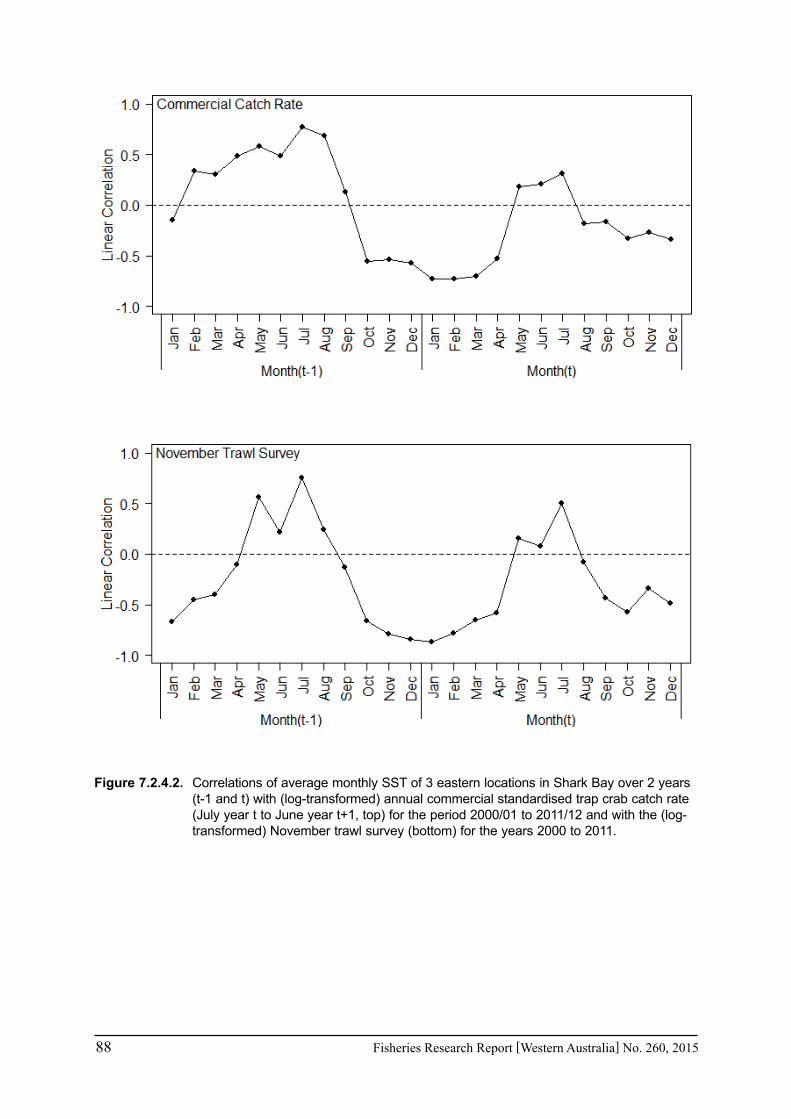
88 Fisheries Research Report [Western Australia] No. 260, 2015
Figure 7.2.4.2. Correlations of average monthly SST of 3 eastern locations in Shark Bay over 2 years (t-1 and t) with (log-transformed) annual commercial standardised trap crab catch rate (July year t to June year t+1, top) for the period 2000/01 to 2011/12 and with the (log-transformed) November trawl survey (bottom) for the years 2000 to 2011.
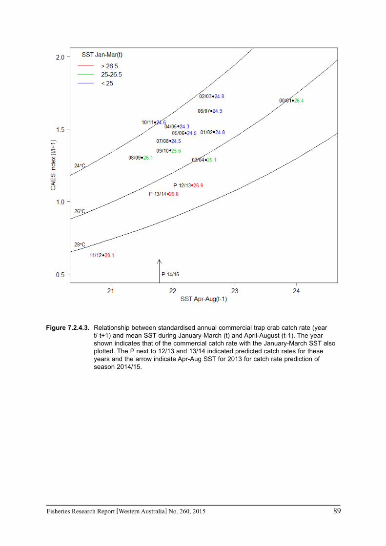
Fisheries Research Report [Western Australia] No. 260, 2015 89
Figure 7.2.4.3. Relationship between standardised annual commercial trap crab catch rate (year t/ t+1) and mean SST during January-March (t) and April-August (t-1). The year shown indicates that of the commercial catch rate with the January-March SST also plotted. The P next to 12/13 and 13/14 indicated predicted catch rates for these years and the arrow indicate Apr-Aug SST for 2013 for catch rate prediction of season 2014/15.

90 Fisheries Research Report [Western Australia] No. 260, 2015
Figure 7.2.4.4. Relationship between November trawl survey legal crab catch rate (year t) and mean SST during November (t-1) - February (t). The 2013 catch rate point is also shown but has not been used in the regression analysis.
Shark Bay scallop fishery
The Shark Bay scallop fishery has been the largest scallop fishery in WA. The scallops are retained by a dedicated scallop fleet as well as prawn trawlers and both fleets use low-opening otter trawls. A catch arrangement between the two fleets has been determined with the scallop fleet allocated 70% of catch. The principal management tools to protect breeding stock involve controlling fishing effort and ceasing fishing to a target catch rate as well as seasonal and spatial closures. A fishery-independent trawl survey measuring the abundance of 0+ pre-recruits and 1+ residual stock has been conducted about November each year since the early 1980s and is used for catch prediction and the setting of management arrangements in the following fishing season (Joll and Caputi 1995a; Lenanton et al. 2009).
The reproductive cycle in Shark Bay scallop stocks is generally between April/May through to December (Joll and Caputi 1995b). Given the energetic demands of reproduction, food availability for adults as well as larvae may be an important factor in determining the timing

Fisheries Research Report [Western Australia] No. 260, 2015 91
of the reproductive cycle (Joll and Caputi 1995b). The timing of spawning is crucial to ensure temperatures and concentrations of phytoplankton are adequate for larval development (Cragg 2006). Changes in environmental patterns may however, lead to different periods of the spawning cycle having a greater importance as contributors to overall recruitment (Joll and Caputi 1995a).
Saucer Scallops are broadcast spawners, releasing their eggs and sperm into the surrounding waters for fertilisation to occur in the water column (Kailola et al. 1993). During this period larvae are susceptible to being passively transported by tides and currents whilst in the water column. Larval survival is affected by food availability and predator abundance, and the length of the larval period (assuming survival is enhanced by reducing time in the plankton community) can also be influenced by water temperature.
Scallop catches in Shark Bay show the typical large variation associated with scallop fisheries with years of good catches generally occurring the year after El Niño years (Figure 7.2.4.5). The El Niño years usually have a weaker Leeuwin Current and cooler water temperatures that can result in good scallop recruitment (Joll and Caputi 1995a). The stock levels since 2011 appear to have been significantly impacted by the heat wave in the summer of 2010/11 that was influenced by strong La Niña conditions. There are two separate scallop stocks in Shark Bay, one in northern Shark Bay and the other in Denham Sound (Kangas et al. 2012) and the factors affecting the recruitment in these stocks are examined separately.
The first indication of the effect of the heat wave was that the commercial catch in 2011 that started just after the heat wave event was well below the prediction based on the scallop abundance in the fishery-independent survey in November 2010 (Figure 7.2.4.6). This may have been attributed to poor growth and mortality of scallops during marine heat wave in late 2010 and 2011. Fishers also noted that the meat quality was not good in 2011. Scallop fishing was fairly limited in 2011 and stopped in May at a catch rate level that should have ensured an adequate spawning stock in the winter of 2011 and some carryover of stock for the following season. However by August, anecdotal comments from prawn fishers were that there appeared to be very few scallops on the trawl grounds. The annual pre-season survey in November 2011 confirmed the observations with very low recruit abundance and extremely low residual abundance throughout the bay (Figure 7.2.4.6). Due to the very low abundance the scallop fishery was closed for the 2012 season.
Strong La Niña conditions as in 2011 (with strong Leeuwin Current flow and high SST) are always associated with poor scallop larval settlement so the poor recruitment during the November 2011 survey was expected, however the poor survival of residual stock was not. We suspect high mortality of adults from thermal stress, reduced growth from the stress and possibly some change in food availability. The November 2012 pre-season survey again indicated very low recruitment and almost no residual scallops in Shark Bay which means an extremely low spawning stock (Figure 7.2.4.6). The Shark Bay scallop fishery remained closed for the 2013 season.
Spawning mainly occurs in the winter period and the November trawl survey provides an indication of the recruitment. Therefore the relationship between the log-transformed recruitment catch rate in November (year t) and the monthly SST in the previous 18 months (June t-1 to November t) was examined as this covers the period prior to and during the spawning and larval period. The SST relationships were examined for 5 locations where SST data was available for Shark Bay to represent the Northern Shark Bay stock and 2 SST locations near the Denham Sound stock. As the multiple SST locations showed similar results, the average of SST locations for each of the two scallop stocks was used in the assessment.
92 Fisheries Research Report [Western Australia] No. 260, 2015
Examination of the correlations between the annual northern Shark Bay November recruitment index (log transformed) and the monthly SST in the previous two years identified two periods when the negative correlation was highest. The first was in the previous summer period (December-January) which was prior to winter spawning and the second was during the spawning period (April to June) (Figure 7.2.4.7 top). The correlation between the recruitment index and the SST in these two periods was -0.46 (p<0.01) and -0.36 (p<0.05), respectively. The multiple correlation with both periods was 0.52 (p=0.01) with the December-January period being significant (p=0.03) but not the April-June period (Figure 7.2.4.8 top).
The major concern resulting from consecutive years of low recruitment and low residual abundance due to environmental conditions is that the spawning stock has become very low. This may have occurred despite there being no retention of scallops since 2012. A preliminary indication of the level of spawning stock is the combined 0+ and 1+ abundance from the previous November survey as the 0+ are generally mature by the following winter. The stock-recruitment-environment relationship using recruitment data up to 2012 shows that the spawning stock index is not significant in this relationship. However it does show that the spawning stock in 2012 (based on the November 2011 survey) is likely to have been well below historic levels (Figure 7.2.4.9 top). The scallop abundance in the November surveys of 2012 and 2013 show a declining trend that will contribute to the spawning stock and subsequent recruitment in 2013 and 2014, respectively. The 2013 record-low recruitment would have been affected by the low spawning stock as well as the above-average SST in the previous summer of 2012/13. This low abundance will result in a very low spawning stock in the 2014 winter and it is possible that the spawning stock may be so low that a good recruitment in 2014 may not occur irrespective of the environmental conditions.
Assessment of the Denham Sound scallop November recruitment index (log transformed) with the monthly SST in the previous two years also identified similar periods with the highest negative correlations. The first was in the previous spring/summer period (October-December) which was prior to spawning and the second was during the spawning period (June) (Figure 7.2.4.7 bottom). The correlation between the recruitment index and the SST in these two periods was -0.39 (p=0.03) and -0.57 (p=0.001), respectively. The multiple correlation with both periods was 0.67 (p<0.001) with the October-December and June periods being significant (p=0.02 and p<0.001, respectively) (Figure 7.2.4.8).
The stock-recruitment-environment relationship using recruitment data up to 2012 was also examined for Denham Sound using a spawning stock index based on total abundance in Denham Sound November survey of the previous year. The combination of spawning stock index (log transformed) and June SST resulted in a multiple correlation of 0.68 (p<0.001) with the spawning stock index and June SST significant (p=0.01 and p=0.007, respectively) in this relationship. This indicates the spawning stock in 2012 (based on the November 2011 survey) is likely to have been well below historic levels (Figure7.2.4.9) and may have contributed to the low recruitment in 2012. The scallop abundance in the November surveys of 2012 and 2013 show a declining trend that will contribute to the spawning stock and subsequent recruitment in 2013 and 2014, respectively. The 2013 very low recruitment would have been affected by the low spawning stock. This low abundance will result in a very low spawning stock in the 2014 winter and it is possible that the spawning stock may be so low that a good recruitment in 2014 may not occur irrespective of the environmental conditions.
The log index of spawning stock below 4 appears to be the stock abundance that affects recruitment in both the northern Shark Bay and Denham Sound stock (Figure 7.2.4.9). There are two periods
Fisheries Research Report [Western Australia] No. 260, 2015 93
in Denham Sound where the spawning stock was below the log index of 4 for an extended period. The first commenced as a result of a low recruitment in 1984 which resulted in 5 years of low spawning stock and low recruitment until there was a spike in recruitment in 1990. The second period commenced due to low recruitment in 1994 followed by 8 years of low spawning stock and low recruitment until there was a gradual improvement in spawning stock and recruitment during 2000–2003. The recovery of the scallop stocks in Denham Sound in 1990 and during 2000–2003 when the scallop abundance was at a similar level to 2013 provides an indication of how the stocks may recover if there are suitable environmental conditions (Figure 7.2.4.9).
Historically the main focus of the examination of environmental factors affecting the Shark Bay scallop recruitment has been the negative effect of the strong La Niña conditions (which are associated with strong Leeuwin Current flow and high SST) during the winter spawning period (Joll and Caputi 1995a; Lenanton et al. 2009b). However this study has identified the importance of SST during the summer period, prior to spawning, as also being a key period that may be affecting the subsequent spawning and hence recruitment. This summer period has probably become more important as a result of the extreme SST experienced in the last three summers since 2010/11. This result supports the anecdotal reports obtained after the 2010/11 summer marine heat wave on the lack of growth and poor quality meat during this period. This analysis highlights that the highest recruitment in northern Shark Bay has occurred in 1987, 2006 and 2007 when the summer SST was relatively low (<23°C) with poor recruitment occurring in the two recent years, 2011 and 2012), when the SST was above 25°C for the first time (Figure 7.2.4.8).
The summer SST for the summer of 2013/14 of 24.4°C in northern Shark Bay is lower than the previous three years but still above average. However the effect of the consecutive years of low recruitment and apparent reduced survival of residual 1+ stock in recent years will have drastically reduced the spawning stock in both northern Shark Bay and Denham Sound (Figure 7.2.4.9). It may take a number of years of good environmental conditions for the spawning stock to rebuild before a major improvement in recruitment is seen.

94 Fisheries Research Report [Western Australia] No. 260, 2015
Figure 7.2.4.5. Time series of (a) Shark Bay (including Denham Sound) and (b) Abrolhos scallop catches (with ENSO events in the previous year indicated).

Fisheries Research Report [Western Australia] No. 260, 2015 95
Figure 7.2.4.6. Time series of Shark Bay scallop November survey recruitment and residual index by northern Shark Bay grounds and Denham Sound.

96 Fisheries Research Report [Western Australia] No. 260, 2015
Figure 7.2.4.7. Correlations between the annual scallop recruitment index (log transformed) in northern Shark Bay (top) and Denham Sound (bottom) (November year t) and the monthly SST in the previous 2 years.
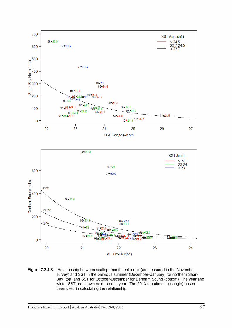
Fisheries Research Report [Western Australia] No. 260, 2015 97
Figure 7.2.4.8. Relationship between scallop recruitment index (as measured in the November survey) and SST in the previous summer (December–January) for northern Shark Bay (top) and SST for October-December for Denham Sound (bottom). The year and winter SST are shown next to each year. The 2013 recruitment (triangle) has not been used in calculating the relationship.
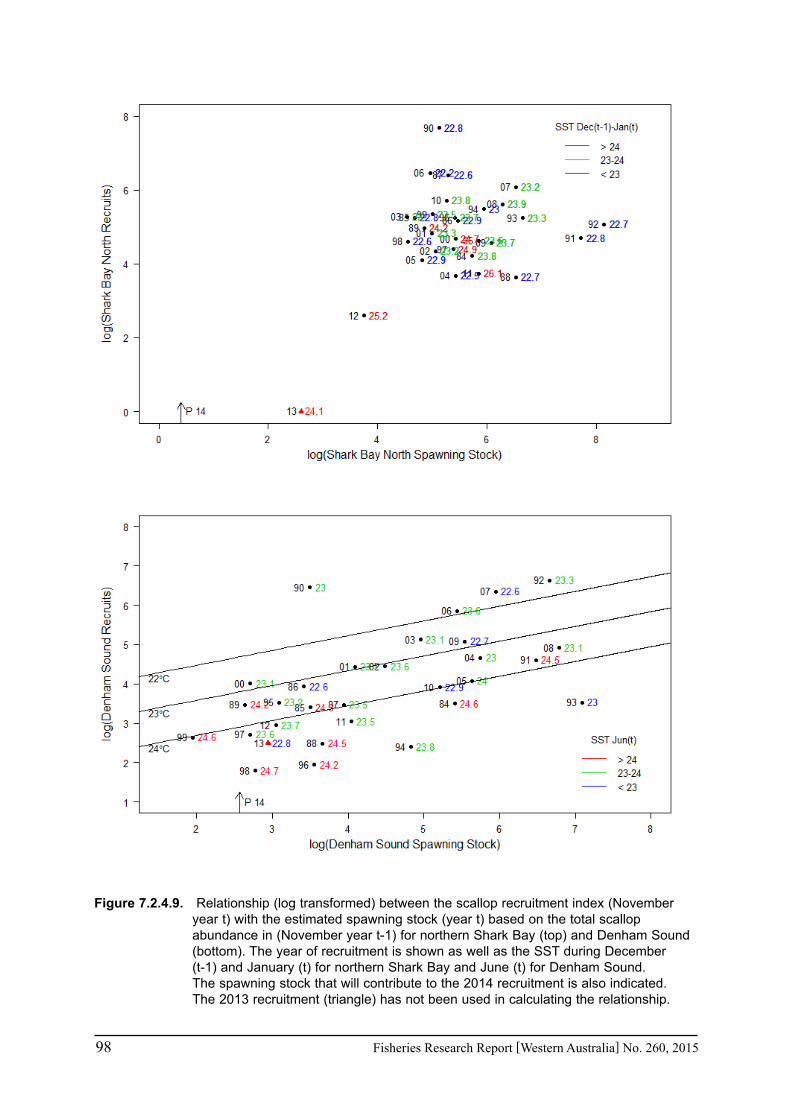
98 Fisheries Research Report [Western Australia] No. 260, 2015
Figure 7.2.4.9. Relationship (log transformed) between the scallop recruitment index (November year t) with the estimated spawning stock (year t) based on the total scallop abundance in (November year t-1) for northern Shark Bay (top) and Denham Sound (bottom). The year of recruitment is shown as well as the SST during December (t-1) and January (t) for northern Shark Bay and June (t) for Denham Sound. The spawning stock that will contribute to the 2014 recruitment is also indicated. The 2013 recruitment (triangle) has not been used in calculating the relationship.

Fisheries Research Report [Western Australia] No. 260, 2015 99
Abrolhos Islands scallop fishery
The Abrolhos Islands and mid-west trawl fishery is fished by dedicated scallop trawlers and is managed similarly to the Shark Bay scallop fishery. It has experienced high variability in annual recruitment and resultant scallop catches as with the Shark Bay scallop fishery that have also been generally associated with ENSO conditions (Figure 7.2.4.5).
The spawning cycle is different in the Abrolhos scallop population compared with Shark Bay in that the spawning period occurs in about September–December at the Abrolhos compared to Apr/May–August in Shark Bay. Therefore the fishery-independent trawl survey that has been conducted about October each year shows only one length frequency cohort that is dominated by scallops that are about 1 year old with some that are 2 years old. This abundance index is used for catch prediction and the setting of management arrangements in the following fishing season (Figure 7.2.4.10).
Similar to Shark Bay, the scallop meat quality in 2011 fishing season was not good and this appears to be the first sign of the effect of the heat wave in the summer of 2010/11. In 2011, 2012 and 2013 the pre-season scallop survey indicated record-low abundances with almost no scallops found in 2012 and 2013 (Figure 7.2.4.10), which has resulted in the fishery being closed since 2012 and will not be opened for the 2014 season.
The correlations between the annual recruitment index (log transformed) in Abrolhos Is. (October each year) and the monthly SST in the previous two years indicated that the highest negative correlation (r=-0.84, (p<0.001) occurred about March in the same year as the survey (Figures 7.2.4.11 and 7.2.4.12). The recruitment indices for 2012 and 2013 were not used in this assessment as they have been affected by very low spawning stock in 2011 and 2012. The correlation assessment was undertaken with and without 2011 and indicates that the correlation with SST over March-June is consistent with and without 2011. However the correlation during November-February was only negative when 2011 was included. March represents the period that the Leeuwin Current strengthens on the lower west coast of Western Australia and passes near the Abrolhos with the scallops being in the early juvenile phase at this time. Water SST above 24°C always results in a relatively low recruitment index of less than 2000, whereas years with the SST less than 24°C have 4 years with good recruitment and 4 years with the lower recruitment (Figure 7.2.4.12). This indicates that cooler SST associated with a weak Leeuwin Current are necessary for good recruitment but that there are other environmental condition(s) that are also required to achieve good recruitment. For example, these additional environmental conditions could be water current movements at the time of spawning which could be on a lunar phase.
As a result of the consecutive years of very low recruitment since 2011, the spawning stock is likely to have been affected so a stock-recruitment-environment relationship was examined. The scallop abundance during the survey in October of the previous year represents a good index of spawning stock as it occurs during the spawning period. The stock-recruitment relationship with March SST as the environmental variable has a multiple correlation of 0.87 (Figure 7.2.4.13) with the spawning stock (p<0.05) and March SST (p<0.001) both significant. It shows that the recruitment in 2012 and 2013 would have been affected by the low spawning stock in the previous year as well as the warm SST in March 2012 and 2013.
The SST for January–February 2014 has returned to average levels so that the March SST is expected to be below 24°C. However the record-low 2013 spawning stock may result in the 2014 recruitment also remaining below average. The key factor determining if and when this fishery recovers is whether there is sufficient spawning stock remaining to enable an improved

100 Fisheries Research Report [Western Australia] No. 260, 2015
recruitment if the appropriate environmental conditions occur. It may require a couple of consecutive years of good environmental conditions to result in an improved spawning stock before the recruitment recovers.
Figure 7.2.4.10. Time series of Abrolhos scallop abundance index in the annual October survey (year Y) and catch in following year (Y+1).
Figure 7.2.4.11. Correlations between the annual scallop recruitment index (log transformed) in Abrolhos Is. (October/November year t) and the monthly SST in the previous 2 years. The recruitment indices for 2012 and 2013 were not used in the assessment as they may have been affected by low spawning stock the previous year. The correlations are undertaken with and without including the 2011 recruitment survey.

Fisheries Research Report [Western Australia] No. 260, 2015 101
Figure 7.2.4.12. Relationship between Abrolhos scallop recruitment index (year t) and SST in March (year t). The recruitment indices for 2012 and 2013 were not used in the assessment as they may have been affected by low spawning stock the previous year.
Figure 7.2.4.13. Relationship between the scallop recruitment index (October year t) with the estimated spawning stock based on the scallop abundance in October year (t-1) for Abrolhos Is. The year of recruitment is shown as well as the SST during March (t). The spawning stock that will contribute to the 2014 recruitment is similar to that shown for 2012 and 2013.

102 Fisheries Research Report [Western Australia] No. 260, 2015
Shark Bay prawn fishery
The Shark Bay prawn fishery is the largest prawn fishery in WA focused on the Western King Prawn (Penaeus latisulcatus) and the Brown Tiger Prawn (Penaeus esculentus). It has a similar management approach to the Exmouth Gulf fishery. Both prawn species exhibit annual variability in landings but in the early 1980s this fishery also experienced recruitment overfishing of Brown Tiger Prawns. In recent years (since 2000), higher recruitment of both species has occurred during strong La Niña/Leeuwin Current years and strong recruitment strength was observed in 2011. This led to good catches and this may have been due to improved catchability, growth and survival of prawns due to the warmer water temperatures associated with the marine heat wave and the turbidity effects of the flooding events.
There were no obvious negative effects of the 2010/11 heat wave on the recruitment of key prawn species in 2011 or 2012. However there was an apparent shift in the distribution of the Brown Tiger Prawns in the eastern part of the bay which is regarded as the key Tiger Prawn spawning area and a very low spawning stock abundance was recorded for 2012 in this area. However commercial catch rates of Brown Tiger Prawn were quite high just south of the Tiger Prawn spawning area indicating that prawns may not have migrated into the historically known spawning area in 2012. This may be a result of the direct effects of the heat wave and/or flooding events or the effects of these environmental conditions on the seagrass habitat.
The life cycle of King and Tiger Prawn occurs over a year with spawning occurring between autumn and spring (King Prawns) and mainly spring (Tiger Prawns) with recruitment to the fishery occurring the following autumn. Therefore fishery-independent recruitment surveys have been undertaken in March and April since 2000 (Figure 7.2.4.14) which enable catch prediction and the management approach (e.g. area openings based on abundance and size of prawns) to be determined. Therefore statistical analyses of Tiger and King Prawn recruitment index during March and April with average monthly SST from three locations in the recruitment area over the previous 24 months were examined to assess the effect of the SST during the heat wave and other time periods.
The recruitment index for King and Tiger Prawns was positively correlated with SST from about October the previous year until the time of the survey in April (Figure 7.2.4.15) with the record-high SST during the 2010/11 period resulting in the highest recruitment index in 2011 (Figure 7.2.4.14). The Tiger Prawn recruitment also recorded negative correlations with SST during the period (May-July) prior to spawning. The relationship between the log-transformed King and Tiger Prawn recruitment index (March-April year t) with the SST during November (year t-1) to April (t) resulted in a positive correlation of 0.628 (p=0.016) and 0.826 (p<0.001) respectively (Figure 7.2.4.16).
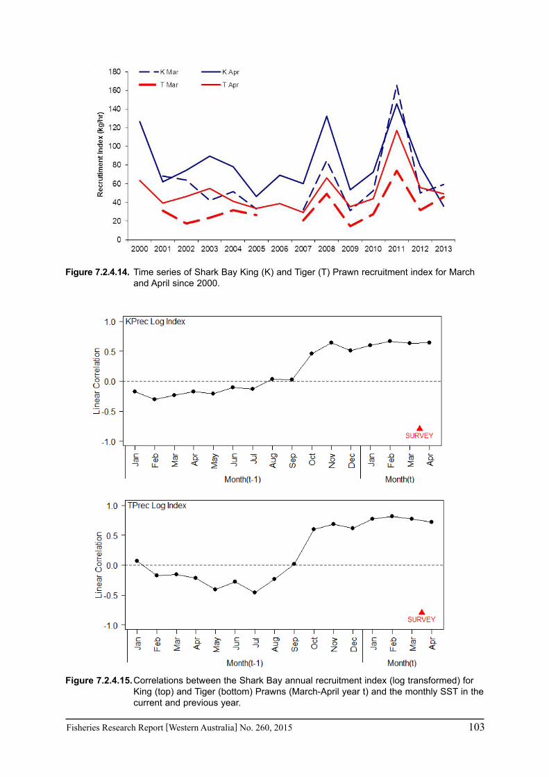
Fisheries Research Report [Western Australia] No. 260, 2015 103
Figure 7.2.4.14. Time series of Shark Bay King (K) and Tiger (T) Prawn recruitment index for March and April since 2000.
Figure 7.2.4.15. Correlations between the Shark Bay annual recruitment index (log transformed) for King (top) and Tiger (bottom) Prawns (March-April year t) and the monthly SST in the current and previous year.

104 Fisheries Research Report [Western Australia] No. 260, 2015
Figure 7.2.4.16. Relationship between Shark Bay King (top) and Tiger (bottom) Prawn recruitment index (March-April year t) and SST (November year t-1 to April year t). The recruitment year is indicated.
Fisheries Research Report [Western Australia] No. 260, 2015 105
Exmouth Gulf prawn fishery
The Brown Tiger Prawn (P. esculentus) can live for over two years although animals greater than two years are rarely caught under current harvesting practices. The prawns become mature at six to seven months of age at a size around 25–28 mm carapace length (Penn and Stalker 1979). Brown Tiger Prawns spawn in the deeper waters and more offshore waters of Exmouth Gulf (Penn and Caputi 1986) and Shark Bay. The planktonic larvae are transported into structured habitats in shallow coastal areas, as postlarvae they settle on beds of seagrass and algae two to four weeks after the eggs are released from the females (Dall et al. 1990; Haywood et al. 1995; Liu and Loneragan 1997). The key spawning period in Exmouth Gulf is between August and October (White 1975; Penn 1980; Penn and Caputi 1986). At spawning the females swim near the bottom releasing the eggs, which float and usually hatch within 24 hours. After hatching from the egg the larvae swim freely in the water column but do not feed. During this stage the larvae utilise stored food from the egg, completing a series of six moults before developing to the next larval stage (Penn and Stalker 1979). Predators are responsible for high mortality rates of the larvae.
The Exmouth Gulf prawn fishery is the second largest prawn fishery in Western Australia (WA). It is based primarily on the Brown Tiger Prawn P. esculentus and the Western King Prawn P. latisulcatus. Management is based on input controls, including limited entry, seasonal and area openings and closures, moon closures and gear controls. Management arrangements are designed to keep fishing effort at levels that will maintain a sufficient spawning biomass of prawns. It incorporates a flexible fishing regime to optimise size and value of prawns. In the early 1980s very low landings were attributed to recruitment overfishing and management strategies were put in place to protect the spawning stock and the landings improved over 3–4 years. Cyclones have also had a major impact, particularly on Brown Tiger Prawns over the history of the fishery. In 1975 very high landings were recorded, attributed to positive cyclone effects whilst in 2000 very low landings were recorded and a recruitment failure was detected – attributed to a severe cyclone that went through the middle of Exmouth Gulf in 1999 and caused significant physical damage to inshore nursery habitats (Loneragan et al. 2013). A fairly strong correlation has been observed with percentage of seagrass/algal cover and Brown Tiger Prawn landings during the recovery of the structured habitats in the inshore areas between 2000 and 2004 (post cyclone).
The heat wave event in 2010/11 may have contributed to the recent extremes in abundance of brown tiger prawns in Exmouth Gulf. In 2011, the Brown Tiger Prawn recruitment and landings were one of the highest recorded which led to a very high spawning stock abundance. However in 2012, the lowest recruitment was observed resulting in the lowest catch. This is turn has resulted in low spawning stock in 2012 although it is at levels that have historically resulted in moderate recruitment.
The hypotheses under investigation are that:
• The 2010/11 warmer summer temperatures may have been beneficial for recruitment in 2011.
• The warmer summer temperatures (which also occurred in the summer of 2012/13) may have had a direct negative effect on the spawning (timing/success) or transport/survival of larvae in the spring of 2011 leading to poor recruitment in 2012. This may be a short-term (1 year) effect as the spawning stock is not significantly affected.
• The warmer temperatures may have led to the loss of structured habitat (seagrass and/or algae) in the nursery areas that may have contributed to the poor recruitment. This may be a long-term (3–4 year) effect based on previous experience in 2000 with loss of structured habitat (Loneragan et al. 2013).

106 Fisheries Research Report [Western Australia] No. 260, 2015
Three fishery-independent recruitment trawl surveys have been undertaken for Tiger Prawns in March and April since the early 1980s (Figure 7.2.4.17) which enable catch prediction and the management approach (e.g. area openings based on abundance and size of prawns) to be determined. Therefore statistical analyses of Tiger Prawn recruitment index during March and April with average monthly SST from two locations over the previous 24 months were examined to assess the effect of the SST during the heat wave and other time periods. As a result of the effect of cyclone Vance on the seagrass in 2000 and 2001 and the suspected effect of the heat wave on the seagrass in 2012 and 2013 then the SST correlation assessment was also undertaken with these years removed.
The recruitment index for Tiger Prawns did not show any significant correlation with SST during the six months prior to the recruitment survey in April (Figure 7.2.4.18). However there was a negative correlation with SST during the months (May–July) prior to spawning. The relationship between Tiger Prawn recruitment index (March–April year t) with the average SST during May–July the previous year resulted in a correlation of -0.588 (p=0.002) (Figure 7.2.4.19).
An assessment of the water temperature effect on the King Prawn was undertaken using April recruitment survey abundance undertaken since 2005 and the SST at two locations within Exmouth Gulf. This showed a negative correlation between the recruitment index and the monthly SST during the spring spawning period, September-December the previous year (Figure 7.2.4.20). The relationship between the April recruitment index and the combined November-December SST resulted in a correlation of -0.62 (p=0.05) (Figure 7.2.4.21). The November-December SST in 2010 and 2013 that influence the 2011 and 2014 recruitment index are two of the three highest SST in over 30 years. The negative relationship with SST is in contrast with the positive relationship between King Prawn recruitment in Shark Bay and SST during October to April. This may reflect the cooler SST experienced in Shark Bay compared to Exmouth. For example, the SST range during March near the time of recruitment survey in Shark Bay was 24–28°C with temperature above 27°C only being recorded since 2011. This SST range resulted in a positive correlation with Tiger Prawn recruitment. However the SST range at the same time in Exmouth was 26–30°C and recruitment-SST correlation was not significant.
0102030405060708090
100
Mea
n ca
tch
rate
(kg/
hr)
Tiger
King
Figure 7.2.4.17. Time series of Exmouth Gulf Tiger and King Prawn recruitment index undertaken during March–April.
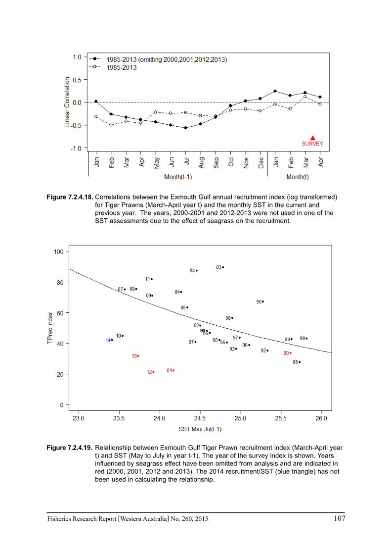
Fisheries Research Report [Western Australia] No. 260, 2015 107
Figure 7.2.4.18. Correlations between the Exmouth Gulf annual recruitment index (log transformed) for Tiger Prawns (March-April year t) and the monthly SST in the current and previous year. The years, 2000-2001 and 2012-2013 were not used in one of the SST assessments due to the effect of seagrass on the recruitment.
Figure 7.2.4.19. Relationship between Exmouth Gulf Tiger Prawn recruitment index (March-April year t) and SST (May to July in year t-1). The year of the survey index is shown. Years influenced by seagrass effect have been omitted from analysis and are indicated in red (2000, 2001, 2012 and 2013). The 2014 recruitment/SST (blue triangle) has not been used in calculating the relationship.
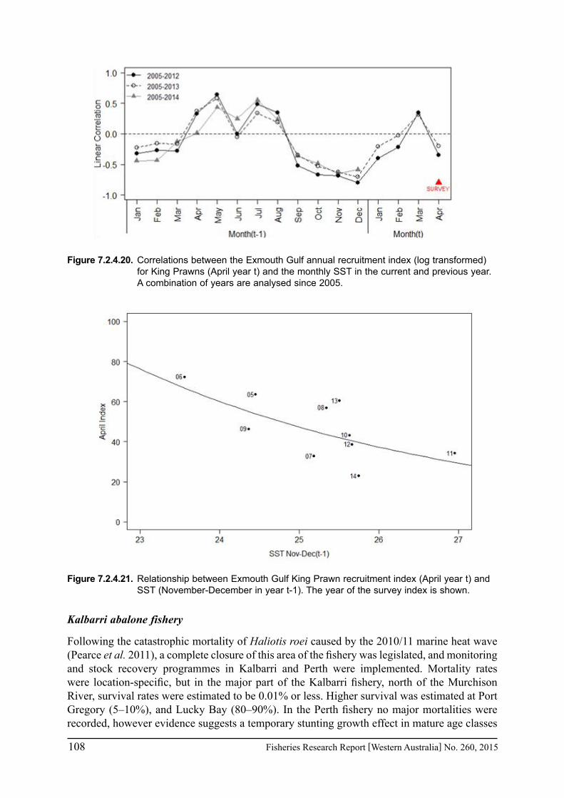
108 Fisheries Research Report [Western Australia] No. 260, 2015
Figure 7.2.4.20. Correlations between the Exmouth Gulf annual recruitment index (log transformed) for King Prawns (April year t) and the monthly SST in the current and previous year. A combination of years are analysed since 2005.
Figure 7.2.4.21. Relationship between Exmouth Gulf King Prawn recruitment index (April year t) and SST (November-December in year t-1). The year of the survey index is shown.
Kalbarri abalone fishery
Following the catastrophic mortality of Haliotis roei caused by the 2010/11 marine heat wave (Pearce et al. 2011), a complete closure of this area of the fishery was legislated, and monitoring and stock recovery programmes in Kalbarri and Perth were implemented. Mortality rates were location-specific, but in the major part of the Kalbarri fishery, north of the Murchison River, survival rates were estimated to be 0.01% or less. Higher survival was estimated at Port Gregory (5–10%), and Lucky Bay (80–90%). In the Perth fishery no major mortalities were recorded, however evidence suggests a temporary stunting growth effect in mature age classes

Fisheries Research Report [Western Australia] No. 260, 2015 109
that has now ceased, but resulted in a 30% drop in numbers of the legal size-class (61-70 mm) transitioning from the sub-legal cohort (51–60 mm).
The very low numbers of abalone remaining in the Kalbarri region has made the natural recovery of this stock uncertain. Therefore different research approaches to help rebuild the stocks are being assessed. The translocation from populations in the region and release of hatchery-grown populations are being evaluated.
An Australian Seafood CRC project (2011/762) has commenced on researching the viability of recovering the collapsed abalone stock through translocation and hatchery-reared releases. Five founder populations sourced from the nearest surviving population at Lucky Bay have been set-up in the Kalbarri region. This was followed up by further translocations from the Perth region to assess the effects on the recovery of the stocks. Hatchery-reared releases are planned for the end of 2014. Future monitoring will determine whether this has been successful in initiating recruitment. The hatchery releases of Roei to aid the recovery of the stock follows the success of the release, survival and growth of hatchery-grown Greenlip Abalone in the south-west of WA (CRC project 2009/710).
Discussion and conclusion
The marine heat wave event in the summer of 2010/11 and the above-average summer temperatures in the following two summers, has been shown to have a significant impact on the invertebrate fisheries in the Shark Bay, Exmouth Gulf and the Abrolhos Islands. The heat wave has been described as a unique Ningaloo Niño event due to the unusual alignment of intraseasonal to interdecadal processes, resulting in an unseasonable surge of the Leeuwin Current and the extreme warm condition in the austral summer of 2010/11 (Feng et al. 2013). A key question is whether the above average temperature over the three years is part of a long-term trend. Doi et al. (2013) has indicated the ability to predict Ningaloo Niño events 9 months in advance, although it underestimated its peak amplitude.
The heat wave event has affected the abalone stock in Kalbarri, scallops in Shark Bay and Abrolhos, Blue Swimmer Crabs in Shark Bay, and prawns in Shark Bay and Exmouth Gulf. The heat wave event represents an example of the effect of an extreme environmental event, irrespective of whether it is related to climate change, that has had a major effect on fisheries. Given that extreme events are likely to be more common with climate change, the heat wave provides an opportunity to assess how this has affected the research and management of the fisheries.
The heat wave had an immediate effect of fish kills of a number of species including rock lobster, fish and most notably the nearly 100% mortality of abalone near Kalbarri (Pearce et al. 2011). These fish kills occurred over a two-week period in late February and early March 2011 when the record-high water temperatures at the time were combined with very calm conditions that probably resulted in deoxygenation of the water in a number of areas. The heat wave also had a significant effect on a number of aspects of the marine community over a large area that was affected by the higher SST (Pearce et al. 2011) including the range extension of a number of tropical fish species (see Section 7.2.5).
The next indication of the effect of the heat wave was that the commercial scallop catch in 2011 in Shark Bay (and Abrolhos) that started just after the heat wave event was well below the prediction based on the scallop abundance in the fishery-independent survey in November 2010 (Figure 7.2.4.5). This was attributed to poor growth and mortality of scallops with fishers also reporting poor meat quality. However the major impact on scallop fishery was observed when

110 Fisheries Research Report [Western Australia] No. 260, 2015
the October and November 2011 scallop survey in the Abrolhos and Shark Bay, respectively, showed very low recruitment and poor survival of 0+ scallops that had been left behind after fishing ceased in the middle of the year. This low abundance has resulted in the closure of both fisheries since 2012 with the scallop abundance declining further in surveys in 2012 and 2013. This study has highlighted the negative effect of high SST on recruitment during the 9 months before and during the spawning period. There is also a strong indication that the recruitment is also being affected by the declining spawning stock as a result of the consecutive years of poor recruitment. If this is the case then it may take a number of years of good environmental conditions for the spawning stock to rebuild before a major improvement in recruitment is seen.
The lack of growth and poor meat quality that was observed in both the Abrolhos and Shark Bay scallop fishery may provide the first indication that the subsequent recruitment associated with this year-class may be unsuccessful as a result of the poor quality of the spawning stock. Anecdotal evidence in the Cockburn Sound crab fishery (Danielle Johnston pers. comm.) and the Roei Abalone Perth metropolitan fishery (Anthony Hart pers. comm.) also noted reduced growth followed by poor recruitment the following year.
The Shark Bay crab fishery produced reasonable catches immediately after the summer heat wave in 2010/11 but the abundance dropped rapidly by the middle of the year with a very low recruitment to the fishery in 2011/12. While the warm temperatures during the juvenile phase in the summer showed a negative effect on recruitment, the warm temperatures during the autumn/winter spawning appears to be beneficial to recruitment. Therefore the cause of the low recruitment to the fishery in 2011/12 was a combination of a very cool winter in 2010 followed by the heat wave in the summer of 2010/11. An improvement in survey catch rates occurred in 2012/13 and 2013/14 as winter SST in 2011 and 2012 returned to historic level but the summer SST in 2011/12 and 2012/13 have remained above average but lower than the record high level of 2010/11. This has resulted in a partial opening of the fishery for 2013/14.
The effect of SST and the heat wave, in particular, had some positive and negative effects on the King and Tiger Prawn stocks in Shark Bay and Exmouth Gulf. With the SST in Shark Bay being generally about 2°C cooler than Exmouth and Tiger Prawns being at the southern end of the their range in Shark Bay, a positive relationship between the recruitment of King and Tiger Prawns with SST during October-April was evident in Shark Bay. This resulted in the highest recruitment index in 2011 as a result of the heat wave (Figure 7.2.4.16). A positive relationship between King Prawn catches and the Leeuwin Current (associated with warm SST) has previously been identified (Caputi et al. 1996; Lenanton et al. 2009b).
While the Tiger Prawn recruitment during 2011 in Exmouth Gulf was also very high, there was no evidence of the positive correlation of SST with Tiger Prawn recruitment over the range of higher SST than that observed in Shark Bay. However there is anecdotal evidence that the higher summer SST in 2010/11 may have affected the seagrass and caused a low recruitment in the 2012 and 2013. This would reflect an indirect effect of water temperature change on the Tiger Prawn fishery. Pratchett et al. (2011) suggested that the most immediate effect of climate change on fishes are likely to be indirect, caused by changes in availability of critical habitats. This highlights the importance of monitoring changes in habitat structure for key species that are reliant on key habitats.
The Tiger Prawn recruitment in both Shark Bay and Exmouth in March-April also recorded negative correlations with SST during the previous winter period (May-July) prior to the main spawning peak during late winter/spring. This correlation has not been recorded previously and needs to be monitored further for verification.

Fisheries Research Report [Western Australia] No. 260, 2015 111
The experience in dealing with the heat wave event on the invertebrate fisheries has highlighted the need for early detection of any decline in abundance to enable management and industry to adjust to the lower abundance by reducing catch and effort or even the closure of the fishery. This emphasises the importance of the fishery-independent surveys that were being conducted for the prawn, scallop and crab fisheries, particularly those that provide a pre-recruit measure of abundance. Many fisheries are generally reliant on commercial catch rates to manage the stock so that there in an inherent delay between any decline in abundance and the ability of researchers, managers and industry to react to the change in abundance. This often results in the stocks being overfished and a delay in the recovery of the stocks. With an increased likelihood of changes in the trends of abundance occurring as a result of climate change then there in an increased likelihood of the need for management intervention as a result of these consecutive years of low or high abundance.
Pankhurst and Munday (2011) emphasised the sensitivity of the reproduction and early life history stages of marine fish to water temperature changes. The puerulus settlement in the Western Rock Lobster and heat wave effect on invertebrate fisheries in our study have demonstrated the sensitivity of the reproduction and early life history stages to the recruitment to the fishery.
Two marine heat wave workshops have been held to examine the effect of the heat wave on the marine environment. The first was held in May 2011 about two months after the peak of the heat wave event in February/March 2011 (Pearce et al. 2011). This workshop focused on the oceanographic conditions associated with the event as well as the short-term (1-2 mo.) effects observed such as fish kills and southerly range extension of a number of tropical fish species. The second workshop in March 2013 focused on: (a) the environmental factors that caused the heat wave event and the oceanographic conditions in the following two years; (b) the longer-term (6-24 mo.) effect on fisheries; and (c) the effect on the marine environment such as seagrass/algae habitat, coral communities and range extension of tropical species (Caputi et al. 2014d). Besides the effect on fisheries outlined in this Section and 7.2.5 the heat wave had a considerable effect on other aspects of the marine environment:
• In Jurien Bay, community structure of temperate seaweeds, sessile invertebrates and reef fishes was significantly affected by the warming event with a substantial reduction in the cover of canopy-forming seaweeds (e.g. Kelp Ecklonia radiata), including the 100 km range contraction of Scytothalia dorycarpa. An increase in abundance of reef fishes with a warm-affinity (Chaetodon assarius, Labracinus lineatus and Parma occidentalis) was observed. Preliminary data from 2012 suggest that these reef fish communities are returning towards the pre-perturbed state, but there is little sign of recovery of canopy seaweeds and biogenic habitat structure.
• Surveys of Damselfishes Abudefduf sexfasciatus and A. vaigiensis at Rottnest Is. have shown record recruitment in early 2011 and a large settlement in 2012. There were also first sightings of seven tropical fish species, well south of their normal ranges.
• Preliminary analyses suggest a trend of increasing SSTs in the summer and early autumn in Cockburn Sound over the last 10 years and decreasing seagrass shoot densities.
• Acropora spp. bleached with high subsequent mortality within areas of Ningaloo Reef and Abrolhos Is. in 2011.The coral cover in some areas within Ningaloo (Bundegi and southern areas of Ningaloo) has continued to decrease.
• Breeding participation and success of Little Penguins on Penguin Is. in 2011 was the lowest observed in 20 years. High SSTs in April and May were correlated with poorer breeding.
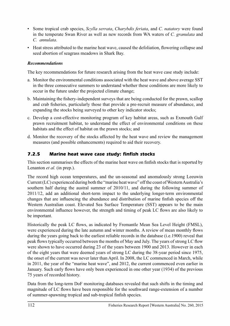
112 Fisheries Research Report [Western Australia] No. 260, 2015
• Some tropical crab species, Scylla serrata, Charybdis feriata, and C. natatory were found in the temperate Swan River as well as new records from WA waters of C. granulata and C. annulata.
• Heat stress attributed to the marine heat wave, caused the defoliation, flowering collapse and seed abortion of seagrass meadows in Shark Bay.
Recommendations
The key recommendations for future research arising from the heat wave case study include:
a. Monitor the environmental conditions associated with the heat wave and above average SST in the three consecutive summers to understand whether these conditions are more likely to occur in the future under the projected climate change;
b. Maintaining the fishery-independent surveys that are being conducted for the prawn, scallop and crab fisheries, particularly those that provide a pre-recruit measure of abundance, and expanding the stocks being surveyed to other key indicator stocks;
c. Develop a cost-effective monitoring program of key habitat areas, such as Exmouth Gulf prawn recruitment habitat, to understand the effect of environmental conditions on these habitats and the effect of habitat on the prawn stocks; and
d. Monitor the recovery of the stocks affected by the heat wave and review the management measures (and possible enhancements) required to aid their recovery.
7.2.5 Marine heat wave case study: finfish stocks
This section summarises the effects of the marine heat wave on finfish stocks that is reported by Lenanton et al. (in prep.).
The record high ocean temperatures, and the un-seasonal and anomalously strong Leeuwin Current (LC) experienced during both the “marine heat wave” off the coast of Western Australia’s southern half during the austral summer of 2010/11, and during the following summer of 2011/12, add an additional short-term impact to the underlying longer-term environmental changes that are influencing the abundance and distribution of marine finfish species off the Western Australian coast. Elevated Sea Surface Temperature (SST) appears to be the main environmental influence however, the strength and timing of peak LC flows are also likely to be important.
Historically the peak LC flows, as indicated by Fremantle Mean Sea Level Height (FMSL), were experienced during the late autumn and winter months. A review of mean monthly flows during the years going back to the earliest reliable records in the database (i.e.1900) reveal that peak flows typically occurred between the months of May and July. The years of strong LC flow were shown to have occurred during 23 of the years between 1900 and 2013. However in each of the eight years that were deemed years of strong LC during the 38-year period since 1975, the onset of the current was never later than April. In 2008, the LC commenced in March, while in 2011, the year of the “marine heat wave”, and 2012, the current commenced even earlier in January. Such early flows have only been experienced in one other year (1934) of the previous 75 years of recorded history.
Data from the long-term DoF monitoring databases revealed that such shifts in the timing and magnitude of LC flows have been responsible for the southward range-extension of a number of summer-spawning tropical and sub-tropical finfish species.

Fisheries Research Report [Western Australia] No. 260, 2015 113
The movements of legal-sized adults and large juveniles of economically important species are immediately reflected in the catch records of commercial and recreational fishers. Spanish Mackerel (Scomberomorus commerson) has historically been an irregular visitor to waters off the Perth Metropolitan area during the warmer months (late summer/autumn). Records available since the “marine heat wave” have revealed a wider distribution in Metropolitan waters, with the first records of this species from protected embayment waters of Cockburn Sound, and a presence in the Metropolitan waters beyond the warmer months of the year. This species was also transported well south of Perth with confirmed reports of capture as far south as Margaret River and Albany on the south coast in the autumn of 2011.
While new recruits of more sedentary demersal tropical and sub-tropical species displaced south of their normal range typically do not survive the cooler inshore winter water temperatures, the marked increase in abundance of species such as the subtropical Western Butterflyfish (Chaetodon assarius) is indicative of a strong response to the changing environmental conditions that delivered additional individuals to more southerly locations.
It is postulated that conditions such as persistent warmer SST have enabled individuals of some other tropical species such as Sand Bass (Psammoperca waigiensis) to over-winter successfully in the inshore habitat (waters > 20 m depth). While the Common Dart (Trachinotus botla), the Smallspotted Dart (T. baillonii), and the Striped Threadfin (Polydactylus plebeius) have over-wintered within the nearshore habitat (waters of 0-20 m depth). However although evidence is available to show that individuals of T. botla have grown to exceed the length at maturity, their gonads remained undeveloped. This is in contrast to another nearshore species, the tropical Rabbitfish (Siganus sp., NB. Black Rabbitfish Siganus fuscescens and Whitespotted Rabbitfish S. canaliculatus are now viewed as synonyms) which has been shown to survive consecutive winters of warmer nearshore SST to mature and establish new viable breeding populations well south of the historical southern limits of the species distribution. This species now contributes to both commercial and recreational catches taken from the marine waters off metropolitan Perth, over 600 km to the south of the former southern limits of the breeding population of this species.
It is important to recognise that it was only possible to use the examples cited above because of the availability of records of the capture of individuals of these species obtained from community ‘web-based’ internet sites. In contrast, existing ‘traditional’ DoF databases such as those relating to commercial catch and effort and recreational fishing surveys were not as useful as other ‘research’ sources such as the nearshore finfish recruitment surveys because they were not designed to record small catches of unusual species. The recently launched Redmap Australia website that allows the public to submit observational data (including photographs) of marine species occurring outside their known distribution proved to be very useful. However, currently it is difficult to determine how representative such web-based community databases are of the real relative abundance of the species they record. It thus is very important that DoF continues to provide on-going support for Redmap Australia, maintains existing research surveys (e.g. nearshore finfish recruitment surveys) and works to develop additional surveys that are able to gather data, to continue to track changes to the distribution and abundance of marine taxa (including marine ‘pest’ species) into the future.
7.3 Development of management policies
Western Australia (WA) is an ideal location to examine biological and socio-economic implications of climate change as it has a coast line extending from 14 to 35ºS which encompasses

114 Fisheries Research Report [Western Australia] No. 260, 2015
tropical to temperate ecosystems within a single state. The coastal fisheries are managed by one organisation, Department of Fisheries, so there is one governance structure. This section examines climate change implications to the management of fisheries in WA. Madin et al. (2012) has suggested that examining the management implications of these changes before they occur may help to mitigate their negative effects and develop effective adaptive management response strategies.
The marine heatwave event in 2010/11 and the recent long-term decline in the rock lobster puerulus settlement has resulted in researchers, managers and industry having to adapt to the effects of an extreme environmental event and a long-term environmental effect. The different effects on the various fisheries have resulted in a number of different research and management approaches being adopted. These case studies have provided a practical example of management and industry having to deal with major changes to these fisheries that are climate-induced. An assessment of these major case studies as well as the other case studies (Part 2 of this report) have identified some key management issues that need to be considered in adapting to climate change effects on fisheries (Table 7.3.1).
Western Rock Lobster fishery
The Western Rock Lobster puerulus settlement has been below average in the seven years, 2006/07 to 2012/13, including the two lowest settlements in the 40-year time series. A number of these low settlements occurred during years of strong Leeuwin Current in 2008 and 2011 which have typically provided conditions for good settlement. Therefore the low settlement in 2008/09 presented an important challenge to the management of the fishery as it was the lowest settlement in the 40-year time series under what had been historically ‘favourable’ environmental conditions of a strong Leeuwin Current. Settlement stayed below average in 2011/12 and 2012/13 despite egg production being very high, suggesting that other long-term environmental factor(s) dominated in these years. The current assessment indicates that an earlier time of breeding (due to warmer water temperatures) and decline in winter storms are the major contributing factors (Caputi et al. 2014c). These trends in water temperatures and winter storms have been occurring for at least 35-40 years (Pearce and Feng 2007; IOCI 2012) and are likely to continue (Section 7.1.3).
The initial focus of management was to adjust management settings to ensure that the downturn in puerulus settlement in combination with heavy fishing pressure did not result in the egg production being driven to unsustainable levels. Stock assessment modelling indicated that continued heavy fishing would result in the egg production reference level of the harvest strategy being breached within a few years. The early warning of the downturn in recruitment to the fishery provided the opportunity for a pro-active management response before these year-classes entered the fishery (there is a 3-4 year lag between settlement and recruitment to the fishery). The management changes resulted in a significant reduction in fishing effort (ca. 40-70%) which commenced in 2008/09. These effort reductions were introduced in years when recruitment to the fishery was still good. They resulted in a significant increase in fishable biomass and very high catch rates during these two years as well as supporting the fishery during the following years with predicted low recruitment (to the fishery), which commenced in 2010/11 (Reid et al. 2013). The fishery management was also changed from input control to an output-control fishery using individual transferable quotas (ITQs) in 2010/11.
The level of effort reductions implemented from 2008/09 were also commensurate with the level of effort reductions estimated at about 50-70% of 2007/08 effort to produce maximum economic yield (MEY) in the fishery (Reid et al. 2013). These changes have also resulted in management and industry discussing the possibility of setting a target harvest rate for the

Fisheries Research Report [Western Australia] No. 260, 2015 115
fishery taking into account the more-conservative MEY assessment (Department of Fisheries 2013). The fishery has had a biological reference point based on egg production since the mid-1990s which has been valuable in the management settings under the low puerulus settlement.
While a change in the recruitment abundance is the key factor in the stock assessment, changes in other biological parameters can also affect the assessment of fisheries. Increasing water temperatures have resulted in a decrease in size at maturity and the size of migrating lobsters from shallow to deep water (Caputi et al. 2010b). These climate change effects have been taken into account in the stock assessment model (de Lestang et al. 2012). Most fishery models generally assume that biological parameters do not change over the years (stationarity assumption) and they generally assume an average level of recruitment when making projections. These stationarity assumptions may become less robust under climate change scenarios. Long-term changes in the abundance of fish stocks, particularly declines, require an appropriate adjustment of fishing effort or catch quota, for the stocks to be managed sustainably. Norman-López et al. (2013) also assessed the potential effects of high risk effects of climate change on the catch of the Torres Strait tropical lobster through modifications of the stock assessment model.
The change in the size of migration due to environmental factors (Caputi et al. 2010b) and reduced level of fishing in recent years may have altered the distribution of lobsters between management zones, Abrolhos (Zone A) and North Coastal Zone (B). The approach applied in recent years to deal with this issue has been to fix the share of the quota between the two zones based on their historic share. The formalization of this approach is being undertaken as part of the harvest strategy proposal for discussion with industry (Department of Fisheries 2013).
The Western Rock Lobster fishery provides an example of a management adaptation response to the long-term decline in puerulus settlement. Catch and fishing effort were reduced to ensure that there was a carryover of stock into the years when the poor year-classes entered the fishery and that the spawning stock remained at sustainable levels.
Marine heat wave effect on fisheries
The heat wave event caused massive fish and invertebrate kills (particularly Roei Abalone in the Kalbarri region) at the time of the event. The abalone fishery in this region has been shut and the very low numbers of abalone remaining has made the natural recovery of this stock uncertain. Therefore different approaches to help rebuild the stocks such as translocation from surviving populations in the region and the release of hatchery-grown populations are being evaluated. One aspect that needs to be evaluated as part of this restocking research is the likelihood of the reoccurrence of the marine heat wave and what is the long-term viability of the stock in this region under climate change.
The heat wave did not appear to have an immediate effect on the mortality of crabs and scallops in Shark Bay as the effects were not observed until about 6 month later. The annual pre-recruitment survey of scallops that has been undertaken since 1982 proved valuable for managers and the fishing industry in the early detection of this poor scallop recruitment year class and adult abundance, so that management and commercial industry decisions were made about the 2012 fishing season before fishing was started. The abundance of Shark Bay crabs in the deep water region of Shark Bay has also been monitored since 2000 which was also valuable in confirming the downturn of this fishery.
The effect of the heat wave on the abalone, scallop and crab populations has not only affected the catches in these fisheries but has also affected the spawning stock. This is particularly evident in for the abalone stocks in Kalbarri and the scallop populations in the Abrolhos and Shark Bay (Section 7.2.4). The low spawning stock may affect the future recruitment in these

116 Fisheries Research Report [Western Australia] No. 260, 2015
fisheries until favourable environmental conditions occur possibly for a number of years and the spawning stock improves. When the spawning stock is below biological reference levels the fishery is typically classified as ‘overfished’. This classification gives the impression to the community that fishing has caused the decline in spawning. Therefore it is important to understand the primary cause of the low spawning stock and identify situations when heavy fishing pressure has resulted in a decline in spawning stock compared to situations when environmental conditions were the main cause of the low spawning stock. That is, even if fishing was significantly reduced (or the fishery closed) the spawning stock would still fall below target reference levels. In both cases the spawning stock would be classed as ‘unacceptable’ and requiring management but it is not appropriate to refer to spawning stock in both situations as ‘overfished’. When spawning stock has been strongly affected by environmental factors such as the heat wave then they are being classified as ‘environmentally limited’ rather than overfished.
The heat wave also resulted in far-reaching range extensions of many tropical finfish species down the west coast and eastwards towards the Great Australian Bight. The recreational fishery adapts quickly to these range extensions but they have not required any management intervention at this stage. The movements of adults and large juveniles of species such as Spanish Mackerel (Scomberomorus commerson) and the subtropical Western Butterflyfish (Chaetodon assarius) is indicative of a strong response to the changing environmental conditions that delivered additional individuals to more southerly locations. The new recruits of more sedentary demersal tropical and sub-tropical species displaced south of their normal range typically do not survive the cooler inshore winter water temperatures. However conditions such as persistent warmer SST may have enabled individuals of some other tropical species such as Sand Bass (Psammoperca waigiensis) to over-winter successfully in the inshore habitat (waters > 20 m depth). Another nearshore species, the tropical Rabbitfish has been shown to survive consecutive winters of warmer nearshore SST to mature and establish new viable breeding populations well south of the historical southern limits of the species distribution. This species now contributes to both commercial and recreational catches taken from the marine waters off metropolitan Perth, over 600 km to the south of the former southern limits of the breeding population of this species.
Risk assessment
This risk assessment approach examined the sensitivity and the likely exposure of stocks to climate change and helps to identify species that have the highest risk of being affected by climate change. The risk assessment was then combined with socio-economic effects of the fisheries to determine species with the highest priority for close monitoring and further investigation for climate change adaptation by management and industry.
The sensitivity assessment (Pecl et al. 2011) of 35 of WA’s key commercial and recreational finfish (23) and invertebrate (12) species identified Perth Herring, abalone species, Black Bream, Western Rock Lobster, Pink Snapper, Whiskery Shark, Tiger Prawn, Pearl Oyster, Bight Redfish, and Australian Herring, as the most sensitive to climate change (Table 7.2.2.1). These 10 species with the highest sensitivity covered the four marine bioregions of WA (North Coast, Gascoyne, West and South Coast) as well as having crustacean, molluscs and finfish representation. The species identified as having the lowest sensitivity were Octopus, Eightbar Grouper, Spanish Mackerel and Red Emperor.
The risk assessment that also takes into account the exposure of the species to climate change identified that species with the highest risks were Perth Herring, Roei Abalone, Black Bream, Western Rock Lobster, Pink Snapper, Whiskery Shark, Tiger Prawns, scallops, Blue Swimmer Crabs and Australian Herring, as having the highest risk to climate change (Table 7.2.2.3).

Fisheries Research Report [Western Australia] No. 260, 2015 117
After taking into account the socio-economic importance of the stocks, the fisheries with highest priority for monitoring and assessment for climate change adaptation were the inshore demersal finfish stocks on the west coast bioregion (Snapper and Whiskery Sharks) followed by the Western Rock Lobster fishery. Other inshore demersal stocks (including Baldchin Groper, Dhufish, Thickskin Shark, Spangled Emperor) and nearshore finfish stocks in the west coast (including Australian Herring and Tailor) were also identified has having high priority. Invertebrate species (prawns, scallops and crabs) in the Gascoyne region recorded the next highest priority.
The risk assessment for climate change fits in with the risk assessment for the ecosystem-based fisheries management (EBFM) that is conducted by the Department of Fisheries at the regional level (Fletcher et al. 2010; 2012) and provides a basis for priority setting for research and management by the Department in WA. Grafton (2010) emphasizes that as a result of greater variability in stocks and the increased uncertainty associated with climate change effects, the risk assessment associated with sustainability may be increased due to increased likelihood of changing environmental conditions.
Case studies
Many of the key management issues highlighted in the case studies focus on the changes in abundance and distribution of species, particularly in cases where there are fixed management zones (Table 7.3.1). The potential range extension or shift south of tropical species such as Spanish Mackerel and Eightbar Grouper, or range contraction for more temperate species such as Pink Snapper will require management assessment of the zones and changes in catch and/or effort allocation between zones. The range extension may also result in species abundance increasing in areas where the species has not been fished previously and may require new allocation of rights.
Potential changes in spatial and temporal distribution of spawning such as that projected for Tailor, Eightbar Grouper and Spanish Mackerel, may require particular attention from researchers and managers to ensure long-term sustainability of the stock is maintained.
Climate change effect on abundance and distribution of stocks are generally the main focus of research, management and industry as they are readily observed by catch and catch rate changes between the different areas. However changes in biological parameters such as growth and size at maturity are also likely to occur with increasing water temperatures and these are not typically monitored on a regular basis. The Western Rock Lobster provides an example of these biological changes occurring as measured by the commercial monitoring program and annual fishery-independent surveys. These biological changes may require changes in the stock assessment modelling and changes in management such as minimum size regulations.
Pre-recruit abundance
The major case studies have highlighted the value of having a reliable pre-recruit abundance for an appropriate early management adaptation response. The pre-recruit information in the rock lobster and scallop fisheries were invaluable for the early detection of changes in abundance that allow for proper stock assessment and management recommendations before fishing takes place on the poor year classes. In the case of the Western Rock Lobster the lag between the timing of the pre-recruit estimate and the fishery is 3-4 years whereas for scallops and crabs the lag is only 3-6 months but nonetheless proved invaluable for early management intervention. These pre-recruit measures also enable early planning of the fishing industry on the level of fishing (and catch) that is likely to occur in the coming season.

118 Fisheries Research Report [Western Australia] No. 260, 2015
Pre-recruit abundance is monitored for most of the key invertebrate fisheries in WA and factored into the management process of the fisheries (Caputi et al. 2014a). These are valuable for the annual stock assessment and management settings for these fisheries but are particularly valuable in detecting long-term trends in recruitment that are more likely to occur as a result of long-term climate change effects on the environment. They provide a basis for early management intervention which can be critical in avoiding the spawning stock from reducing to critical levels.
If direct pre-recruitment monitoring is not possible or cost-effective for some finfish stocks then monitoring of year-class strength via age structure monitoring should be considered. This provides valuable information to assess climate change effects on recruitment strength and enables an assessment of spawning biomass trend.
Harvest strategies
The development of robust harvest strategies and control rules (HSCR) are valuable in ensuring that annual management settings are appropriate based on the information from the key indicators such as egg production and harvest rate. They provide a basis for an agreed method of adjusting catch quotas and/or effort to a level that is commensurate with the stock abundance indicators. The Department of Fisheries (WA) has prepared a draft harvest strategy policy for aquatic resources of WA for industry consultation. Harvest strategies are particularly valuable if the fishery is rated as highly sensitive to climate change as there may be an increased likelihood of long-term trends in the abundance indicators that may require adjustment in catch quota or effort levels. As fisheries in WA are being subjected to a pre-assessment under the Marine Stewardship Council (MSC), the formalisation of the harvest strategies has been a key component of that process. Sumaila et al. (2011) emphasize that fisheries that have been successfully managed to achieve resource sustainability will be better positioned to respond to climate change.
While harvest strategies based on reference points are currently considered best practice management methods, this approach will have to be updated to take into account changing productivity, stock potential and ecosystem changes (Fulton 2011). King and McFarlane (2006) suggest using regime-specific harvest rates that reflect the relative levels of productivity associated with any climate change regime shift. This approach produced the best balance between benefits such as high yields and trade-offs such as minimising fishery-closures and allowed for stock rebuilding when productivity improved. However Walters and Parma (1996) demonstrated that constant fraction harvest policies performed well under strongly autocorrelated annual recruitment which is more likely to occur under climate change. The harvest strategies are even more valuable if they are based on projected trends in recruitment using pre-recruit abundances (Caputi et al. 2014a) as the management settings are then based on the expected level of recruitment rather than the historic level of recruitment.
McIlgorm et al. (2010) highlight that the governance process in dealing with climate change issues is generally slow moving as it has been built on the foundations of a stable decision environment and consistent expectations. They suggest that governance will need to acknowledge the uncertainty that may be associated with climate change effects and be able to adjust to episodic changes. Rigid and complex management controls may restrict the ability of management authorities to adapt to change (McIlgorm et al. 2010). The effect of environmental conditions on the Western Rock Lobster fishery and heat wave effect on a number of fisheries in the mid-west region in WA illustrated the ability of research, management and industry in Western Australia to deal with significant changes in the fisheries as discussed in the case studies above. The fact that research and management are in one agency, Department of Fisheries
Fisheries Research Report [Western Australia] No. 260, 2015 119
(WA), enabled better communication and coordination of research and management activities to deal with the urgent stock assessment and management issues associated with changes. A FAO workshop on climate change and fisheries recognized the importance of learning the lessons of past management practices in response to climate variability and extreme events in designing robust and responsive management system (FAO 2008).
Grafton (2010) suggests that the actual impact of climate change can be reduced by promoting resilience so as to reduce system sensitivities. Reducing levels of fishing such that there is a wider distribution of aged cohorts and a larger exploitable biomass may provide a buffer in the face of unexpected shocks. The adoption of the maximum economic yield as the target for the Western Rock Lobster fishery has resulted in a greater carryover of legal lobsters and hence a wider distribution of ages as a buffer for the years of low puerulus settlement and has also resulted in a very high spawning stock compared to historical levels (Caputi et al. 2014b). This provides an example of increased resilience of the biological as well as the socio-economic system to climate change for this fishery.
While Marine Parks with sanctuary zones are often suggested as an important strategy to improve resilience to climate change (Grafton 2010; Cheung et al. 2012), Department of Fisheries (WA) has promoted development of proper harvest strategies that have sufficient flexibility to be able to respond to changes in abundance as may occur with climate change (Penn and Fletcher 2010). These harvest strategies can sometimes include permanent and/or temporary closed area as part of the harvest strategy if it is deemed appropriate to protect recruitment and/or spawning stock grounds.
Recommendations
This study has identified that climate variability such as long-term trends, decadal shifts and extreme events is having the most impact on fishery stocks and therefore requiring a strategic management response. Therefore meeting the challenge of climate change will require fisheries management arrangements to be flexible enough to rapidly respond to climate variability and will be dependent on early detection of environmental changes and the effects of these changes on stocks, particularly pre-recruit abundances; and (c) having the governance and harvest strategy and control rules (HSCR) in place to enable appropriate and timely responses to changes in stock abundance. Therefore the key management recommendations arising from the climate change study include:
a. Monitoring of key environmental variables and habitat be continued or established so that changes in environmental conditions that may affect fish stocks are identified as soon as possible;
b. Expand the fishery-independent surveys that are being conducted for many fisheries in WA, particularly those providing a pre-recruit measure of abundance, to other key indicator stocks, to provide reliable indicators of stock abundance trends;
c. Implement HSCR for all key fisheries and ensure that they are sensitive to abundance changes that may occur under climate change and their governance allows for management to respond in a timely fashion;
d. Include pre-recruit measures of abundance, if available, in the HSCR to ensure pro-active management of any changes in abundance;
e. Review the fixed zones of fisheries and the implications of any long-term changes in distribution of stock abundance;
f. Consider management implications of range extension of tropical species and who may be entitled to fish the stocks or whether these are regarded as new developing fisheries;
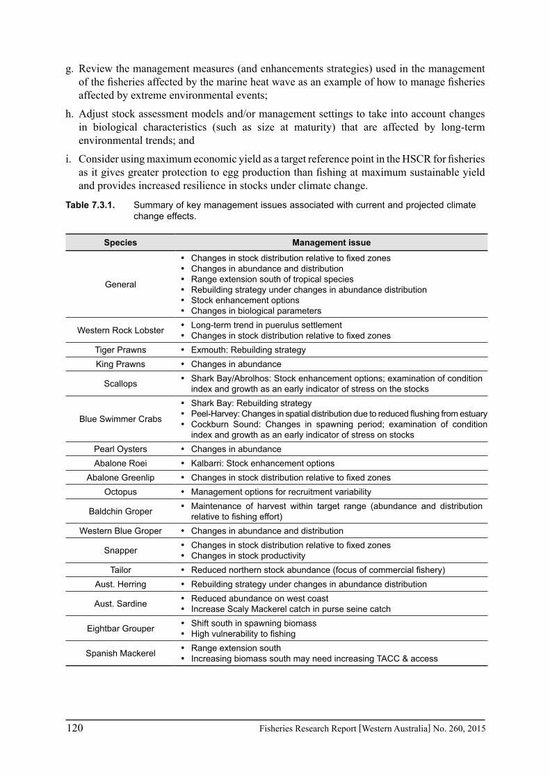
120 Fisheries Research Report [Western Australia] No. 260, 2015
g. Review the management measures (and enhancements strategies) used in the management of the fisheries affected by the marine heat wave as an example of how to manage fisheries affected by extreme environmental events;
h. Adjust stock assessment models and/or management settings to take into account changes in biological characteristics (such as size at maturity) that are affected by long-term environmental trends; and
i. Consider using maximum economic yield as a target reference point in the HSCR for fisheries as it gives greater protection to egg production than fishing at maximum sustainable yield and provides increased resilience in stocks under climate change.
Table 7.3.1. Summary of key management issues associated with current and projected climate change effects.
Species Management issue
General
• Changes in stock distribution relative to fixed zones• Changes in abundance and distribution • Range extension south of tropical species• Rebuilding strategy under changes in abundance distribution• Stock enhancement options• Changes in biological parameters
Western Rock Lobster • Long-term trend in puerulus settlement• Changes in stock distribution relative to fixed zones
Tiger Prawns • Exmouth: Rebuilding strategyKing Prawns • Changes in abundance
Scallops • Shark Bay/Abrolhos: Stock enhancement options; examination of condition index and growth as an early indicator of stress on the stocks
Blue Swimmer Crabs
• Shark Bay: Rebuilding strategy• Peel-Harvey: Changes in spatial distribution due to reduced flushing from estuary• Cockburn Sound: Changes in spawning period; examination of condition
index and growth as an early indicator of stress on stocksPearl Oysters • Changes in abundanceAbalone Roei • Kalbarri: Stock enhancement options
Abalone Greenlip • Changes in stock distribution relative to fixed zonesOctopus • Management options for recruitment variability
Baldchin Groper • Maintenance of harvest within target range (abundance and distribution relative to fishing effort)
Western Blue Groper • Changes in abundance and distribution
Snapper • Changes in stock distribution relative to fixed zones• Changes in stock productivity
Tailor • Reduced northern stock abundance (focus of commercial fishery)Aust. Herring • Rebuilding strategy under changes in abundance distribution
Aust. Sardine • Reduced abundance on west coast• Increase Scaly Mackerel catch in purse seine catch
Eightbar Grouper • Shift south in spawning biomass• High vulnerability to fishing
Spanish Mackerel • Range extension south• Increasing biomass south may need increasing TACC & access

Fisheries Research Report [Western Australia] No. 260, 2015 121
8.0 Benefits and adoption
The main beneficiaries of the study are the commercial and recreational fishers, industry, managers and scientists with some results of the project being presented to all these groups (see details below). The assessment of the relative sensitivity and risk of climate change effects on finfish and invertebrate stocks, combined with the socio-economic importance of the fishery, has helped to prioritize the key stocks that need to be monitored carefully to see if there are any significant trends occurring to their recruitment, spatial distribution and other biological parameters. The case studies have identified some current and potential management issues may affect fisheries.
The assessment of the possible contribution of long-term environmental factors to the recent seven years of low puerulus settlement enables researchers to factor the low settlement into their stock assessment modeling so that management and industry can take this into account in future planning. The stock assessment model has also adopted changes to size of maturity and size of migrating lobsters into the assessment. The management of the fishery has been pro-active in its adaptation to the low puerulus settlement by implementing early management actions to reduce fishing effort and catch before the low puerulus year classes recruited to the fishery. This has resulted in spawning stock being protected from the effects of fishing on the low recruitment as well as achieving a carry-over of legal lobsters into the poor year-class years. The management changes have also resulted in the fishery moving to an individual transferable quota management system and fishing at a level that is achieving maximum economic yield.
The marine heat wave has provided an example of an extreme event that may or may not be related to climate change. In any case it has provided a case study to see how research, management and industry can deal with this type of event.

122 Fisheries Research Report [Western Australia] No. 260, 2015
9.0 Further Development
The case studies highlighted a number of key gaps in the identification of climate change effects on fisheries (Table 7.2.1.3). These can be summarised as follows and are discussed in more detail below:
a. monitoring key environmental trends such as current strength and directions, temperature, salinity, ocean productivity, dissolved oxygen, pH e.g. supporting the research undertaken by IMOS;
b. monitoring trends in key marine habitats such as seagrass, algae and the environmental effect of cyclones and water temperature on these habitats;
c. downscaling of oceanographic modelling to coastal areas along WA’s coast to assess local coastal climate change effects, particularly in the north-west and south coast of WA;
d. oceanographic research on the cause of the extreme heat wave event of summer of 2010/11 which continued into the following two summers and whether this is part of a long-term trend;
e. monitoring of fish stock recruitment and distribution (and other key biological parameters) for the early detection of climate change effects; and
f. understanding effects of environmental variations on recruitment, distribution and other biological parameters of fish stocks e.g. effects of ocean acidification.
Long-term monitoring of key environmental variables at key locations across WA will provide the first warning signal of environmental changes that may be affecting fisheries. This alerts fisheries scientists, managers and industry about possible changes that may occur in their fisheries. Environmental monitoring was the first warning signal in the case studies involving the long-term trends in SST effects of the puerulus settlement of the Western Rock Lobster fishery and marine heat wave event. While satellite data since the early 1980s provides an indication of SST trends, there is a need to monitor other key environmental variables such as bottom water temperatures, salinity, dissolved oxygen and pH that may affect fisheries. IMOS has set up a number of monitoring stations across Australia that will contribute to this long-term monitoring if it has ongoing support. Department of Fisheries (WA), CSIRO and other research organisations have ongoing environmental monitoring at different locations in WA which are generally focused on SST and salinity. However time series of data are only available for some important variables such as productivity, dissolved oxygen and pH at some discrete national reference stations of IMOS.
The changes in environmental conditions can have a direct effect on the species and/or an indirect effect such as affecting a critical seagrass nursery ground. Understanding the cause of a change in stock abundance in fisheries e.g. SST or habitat, provides greater certainty in developing management approaches to deal with the situation. For example, the decline in recruitment in the Exmouth Gulf Tiger Prawns may be due to changes in habitat structure due to the heat wave. Therefore monitoring the habitat change would provide a validation of the cause and possible recovery time for the recruitment. In some cases annual monitoring of the habitat may be required while for some habitats longer-term monitoring (every 3-5 years) is required to detect trends. Habitat monitoring has been identified as a priority for the Department and this requires cost-effective methods for monitoring habitats.
Oceanographic modelling can also generally provide time series of water current strength and direction at any location and depth since the early 1990s, however, these also need ground truthing with actual observations and calibration between models if the model configurations
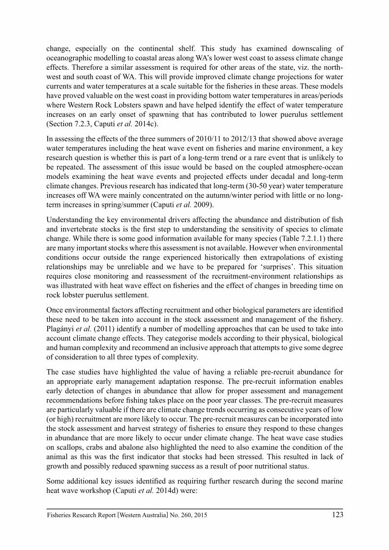
Fisheries Research Report [Western Australia] No. 260, 2015 123
change, especially on the continental shelf. This study has examined downscaling of oceanographic modelling to coastal areas along WA’s lower west coast to assess climate change effects. Therefore a similar assessment is required for other areas of the state, viz. the north-west and south coast of WA. This will provide improved climate change projections for water currents and water temperatures at a scale suitable for the fisheries in these areas. These models have proved valuable on the west coast in providing bottom water temperatures in areas/periods where Western Rock Lobsters spawn and have helped identify the effect of water temperature increases on an early onset of spawning that has contributed to lower puerulus settlement (Section 7.2.3, Caputi et al. 2014c).
In assessing the effects of the three summers of 2010/11 to 2012/13 that showed above average water temperatures including the heat wave event on fisheries and marine environment, a key research question is whether this is part of a long-term trend or a rare event that is unlikely to be repeated. The assessment of this issue would be based on the coupled atmosphere-ocean models examining the heat wave events and projected effects under decadal and long-term climate changes. Previous research has indicated that long-term (30-50 year) water temperature increases off WA were mainly concentrated on the autumn/winter period with little or no long-term increases in spring/summer (Caputi et al. 2009).
Understanding the key environmental drivers affecting the abundance and distribution of fish and invertebrate stocks is the first step to understanding the sensitivity of species to climate change. While there is some good information available for many species (Table 7.2.1.1) there are many important stocks where this assessment is not available. However when environmental conditions occur outside the range experienced historically then extrapolations of existing relationships may be unreliable and we have to be prepared for ‘surprises’. This situation requires close monitoring and reassessment of the recruitment-environment relationships as was illustrated with heat wave effect on fisheries and the effect of changes in breeding time on rock lobster puerulus settlement.
Once environmental factors affecting recruitment and other biological parameters are identified these need to be taken into account in the stock assessment and management of the fishery. Plagányi et al. (2011) identify a number of modelling approaches that can be used to take into account climate change effects. They categorise models according to their physical, biological and human complexity and recommend an inclusive approach that attempts to give some degree of consideration to all three types of complexity.
The case studies have highlighted the value of having a reliable pre-recruit abundance for an appropriate early management adaptation response. The pre-recruit information enables early detection of changes in abundance that allow for proper assessment and management recommendations before fishing takes place on the poor year classes. The pre-recruit measures are particularly valuable if there are climate change trends occurring as consecutive years of low (or high) recruitment are more likely to occur. The pre-recruit measures can be incorporated into the stock assessment and harvest strategy of fisheries to ensure they respond to these changes in abundance that are more likely to occur under climate change. The heat wave case studies on scallops, crabs and abalone also highlighted the need to also examine the condition of the animal as this was the first indicator that stocks had been stressed. This resulted in lack of growth and possibly reduced spawning success as a result of poor nutritional status.
Some additional key issues identified as requiring further research during the second marine heat wave workshop (Caputi et al. 2014d) were:

124 Fisheries Research Report [Western Australia] No. 260, 2015
• The possible effect on the recruitment and adult populations of finfish fisheries needs to be assessed as data becomes available on the age structure of key indicator species such as Snapper.
• The effect of the heat wave and subsequent environmental conditions on the seagrass/algal habitats, coral and the fish community will require ongoing monitoring to assess their recovery.
• Continuing support for Redmap which provides a mechanism for long-term monitoring of the range extension of tropical species such as those observed since the heat wave in 2010/11.

Fisheries Research Report [Western Australia] No. 260, 2015 125
10.0 Planned outcomes
The project outputs have contributed directly to planned outcomes. The progressive and final results of this project have been presented to industry, managers, scientists and community groups as follows:
• Presentations to industry and managers during the annual rock lobster tour meetings with the meetings in 2013 being held at six locations throughout the fishery, from Kalbarri to Fremantle.
• Presentations to industry and managers at a number of Annual Management Meetings conducted for fisheries in Western Australia.
• Presentations to scientists at the International Lobster Conference in Norway, University of WA, Curtin University, Notre Dame University, Murdoch University, Queensland Department of Primary Industry, Climate change conference in Melbourne, Marine Stewardship Council annual audit, ecological risk assessment workshop and Department of Fisheries (WA);
• Presentations to community groups in Busselton and Dunsborough;
• ABC Landline program, ABC 7:30 report, and radio interviews;
• Publication in Nature’s Scientific Reports and related media releases
The key outcomes arising of this project include:
• identification of historical trends in environmental variables and their effects on fisheries;
• downscaling of projected climate change trends of environmental variables in the lower west coast of WA and an assessment of the risk to fisheries;
• an assessment of the sensitivity, exposure and risk ranking of 35 key commercial and recreational fish and invertebrate species so that research, management and industry can take them into account in forward planning;
• taking into account the risk assessment and socio-economic importance of fisheries in the identification of priority fisheries for climate change research and management;
• an evaluation of the effect of an extreme event (marine heat wave) on fisheries and implications for research, management and industry; and
• an evaluation of research, management and industry response to climate change effects on the Western Rock Lobster fishery

126 Fisheries Research Report [Western Australia] No. 260, 2015
11.0 Discussion and Conclusions
This project achieved all three project objectives with some key points arising out of this study discussed under their relevant project objectives.
Objective 1: Assess future climate change effects on Western Australia’s marine environment using a suite of IPCC model projections, downscaled to the key shelf regions and the spatial and temporal scales relevant for key fisheries
Consistent long-term, high-quality monitoring observation in assessing and understanding long term trends in the changing environment is a key component in assessing climate change effects. Many of the longer-term studies to date have been larger-scale observations in open ocean waters beyond the continental shelf, whereas the shallower waters of the continental shelves will perhaps respond more quickly to climate change conditions, and indeed the nearshore environment is of greatest importance to the local community. Such measurements are rare around Australia, including the lengthy and sparsely populated coastline of Western Australia. Apart from the pioneering set of coastal monitoring stations established around Australia by CSIRO in the 1950s which includes the Rottnest Island station, coastal water temperature measurements have tended to be short-term and industry-oriented. The Integrated Marine Observing System (IMOS) aims to meet the need for long-term observations to address research questions, one of which concerns boundary currents and inter-basin flows. There is also a need for some further effort to derive climate trends from proxy data such as coral cores (e.g. Zinke et al. 2014).
The key environmental trends affecting the marine environment in Western Australia (WA) include: (i) changing frequency and intensity of ENSO events; (ii) decadal variability of Leeuwin Current (iii) increase in water temperature and salinity; (iv) change in frequency of storms affecting the lower west coast; and (v) change in frequency and intensity of cyclones affecting the north-west.
Over the past decade or so, there have been more La Niña events than El Niño events, while between the mid-1970s and mid-1990s the reverse was the case. There have been some extended La Niña events, e.g. 1998-2001, 2010-2012 with the 2010-2011 La Niña being one of the strongest this century. These decadal shifts affect the variability and long-term trend of the Leeuwin Current which is essentially driven by the variations and changes of Pacific equatorial easterly winds associated with ENSO and Pacific Decadal Oscillation: the Leeuwin Current has experienced a strengthening trend during the past two decades, which has almost reversed the weakening trend during the 1960s to early 1990s. The Leeuwin Current was especially strong during the recent extended La Niña events, e.g. 1998-2001, and 2010-2012.
A reduction of the Leeuwin Current transport (strength) by 15-20% from 1990s to 2060s is projected under the IPCC A1B scenario. However the climate models tend to underestimate the natural climate variability on decadal and multi-decadal time scales so that while the greenhouse gas forcing induced changes may be obvious in the long-time climate projection, e.g. 2100, for an assessment of short-term climate projection, e.g. 2030s, natural decadal climate variations still need to be taken into account. Decadal climate prediction is still a new front in climate research, and the current climate models only have limited skills in decadal prediction.
The ocean off the lower west coast of WA is one of “hot spots” of SST increases in the Indian Ocean since the 1950s. There are lower rising trends in SST off the northwest and south coasts of Australia. The SST increases to the late 2000s have mostly occurred in autumn-winter off the west coast, at about 0.02-0.035°C per year, compared to little or no increase (<0.01°C per year) in the spring-summer period which has caused a delay in seasonal cycles of SST off the west coast by
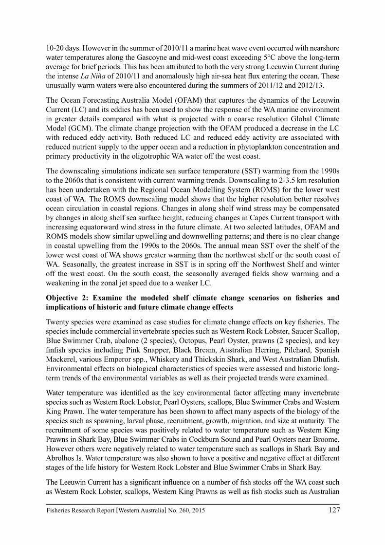
Fisheries Research Report [Western Australia] No. 260, 2015 127
10-20 days. However in the summer of 2010/11 a marine heat wave event occurred with nearshore water temperatures along the Gascoyne and mid-west coast exceeding 5°C above the long-term average for brief periods. This has been attributed to both the very strong Leeuwin Current during the intense La Niña of 2010/11 and anomalously high air-sea heat flux entering the ocean. These unusually warm waters were also encountered during the summers of 2011/12 and 2012/13.
The Ocean Forecasting Australia Model (OFAM) that captures the dynamics of the Leeuwin Current (LC) and its eddies has been used to show the response of the WA marine environment in greater details compared with what is projected with a coarse resolution Global Climate Model (GCM). The climate change projection with the OFAM produced a decrease in the LC with reduced eddy activity. Both reduced LC and reduced eddy activity are associated with reduced nutrient supply to the upper ocean and a reduction in phytoplankton concentration and primary productivity in the oligotrophic WA water off the west coast.
The downscaling simulations indicate sea surface temperature (SST) warming from the 1990s to the 2060s that is consistent with current warming trends. Downscaling to 2-3.5 km resolution has been undertaken with the Regional Ocean Modelling System (ROMS) for the lower west coast of WA. The ROMS downscaling model shows that the higher resolution better resolves ocean circulation in coastal regions. Changes in along shelf wind stress may be compensated by changes in along shelf sea surface height, reducing changes in Capes Current transport with increasing equatorward wind stress in the future climate. At two selected latitudes, OFAM and ROMS models show similar upwelling and downwelling patterns; and there is no clear change in coastal upwelling from the 1990s to the 2060s. The annual mean SST over the shelf of the lower west coast of WA shows greater warming than the northwest shelf or the south coast of WA. Seasonally, the greatest increase in SST is in spring off the Northwest Shelf and winter off the west coast. On the south coast, the seasonally averaged fields show warming and a weakening in the zonal jet speed due to a weaker LC.
Objective 2: Examine the modeled shelf climate change scenarios on fisheries and implications of historic and future climate change effects
Twenty species were examined as case studies for climate change effects on key fisheries. The species include commercial invertebrate species such as Western Rock Lobster, Saucer Scallop, Blue Swimmer Crab, abalone (2 species), Octopus, Pearl Oyster, prawns (2 species), and key finfish species including Pink Snapper, Black Bream, Australian Herring, Pilchard, Spanish Mackerel, various Emperor spp., Whiskery and Thickskin Shark, and West Australian Dhufish. Environmental effects on biological characteristics of species were assessed and historic long-term trends of the environmental variables as well as their projected trends were examined.
Water temperature was identified as the key environmental factor affecting many invertebrate species such as Western Rock Lobster, Pearl Oysters, scallops, Blue Swimmer Crabs and Western King Prawn. The water temperature has been shown to affect many aspects of the biology of the species such as spawning, larval phase, recruitment, growth, migration, and size at maturity. The recruitment of some species was positively related to water temperature such as Western King Prawns in Shark Bay, Blue Swimmer Crabs in Cockburn Sound and Pearl Oysters near Broome. However others were negatively related to water temperature such as scallops in Shark Bay and Abrolhos Is. Water temperature was also shown to have a positive and negative effect at different stages of the life history for Western Rock Lobster and Blue Swimmer Crabs in Shark Bay.
The Leeuwin Current has a significant influence on a number of fish stocks off the WA coast such as Western Rock Lobster, scallops, Western King Prawns as well as fish stocks such as Australian

128 Fisheries Research Report [Western Australia] No. 260, 2015
Herring and Australian Salmon, Pilchards and Whitebait. The effect of the current on fish stocks may be due to its influence on water temperature (i.e. higher water temperatures associated with strong Leeuwin Currents), larval advection and productivity associated with eddy structures. Therefore trends in the Leeuwin Current such as the recent decadal strengthening of the current and projected reduction of strength to 2060s are important in understanding the climate change effect on fisheries.
A risk assessment of 35 key commercial and recreational finfish and invertebrate species, was undertaken based on the sensitivity assessment method developed by the South-east Australian Climate Change group and the likely exposure to climate change. The assessment identified Perth Herring, Roei Abalone, Black Bream, Western Rock Lobster, Pink Snapper, Whiskery Shark, Tiger Prawns, scallops, Blue Swimmer Crabs and Australian Herring, as having the highest risk to climate change.
After taking the socio-economic importance into the account the fisheries with the highest priorities were the inshore demersal finfish stocks on the west coast bioregion (Snapper and Whiskery Sharks) followed by the Western Rock Lobster fishery. Other inshore demersal stocks (including Baldchin Groper, Dhufish, Thickskin Shark, Spangled Emperor) and nearshore finfish stocks in the west coast (including Australian Herring and Tailor) were also identified as having high priority. Invertebrate species (prawns, scallops and Blue Swimmer Crabs) in the Gascoyne region recorded the next highest priority.
The marine heat wave event in the Gascoyne and mid-west region of WA during the summer of 2010/11 and the recent seven years of below-average rock lobster puerulus settlement are used as major case studies to examine how researchers, managers and industry have adapted to the results of an extreme environmental event and a long-term environmental effect. The heat wave had a short-term effect of fish kills and temporary range extension of some tropical species moving south as well as a long-term effect on spawning and larval phase of some species. A major immediate effect was the 99% mortality of Roei Abalone in the Kalbarri region. The abalone fishery in this region has been shut and research trials on the translocation of abalone from nearby unaffected areas into the depleted areas and the release of hatchery-reared abalone are being assessed. A longer-term effect has been the reduced recruitment of scallops in Shark Bay and Abrolhos Is. and Blue Swimmer Crabs in Shark Bay. The adult populations of these stocks have also been severely affected. The fisheries for scallops and crabs in this area did not fully operate during 2012 and 2013. The annual pre-recruitment survey of scallops that has been undertaken in Shark Bay since 1982 has proved valuable for managers and the fishing industry in the early detection of this poor scallop recruitment year class and adult abundance so that management and commercial industry decisions were made to not fish in 2012. The abundance of Shark Bay crabs in the deep water region has also been monitored since 2000 and has been valuable in the detection of the downturn of this fishery and fishing ceased from April 2012. While there has been a resumption of limited fishing on Blue Swimmer Crabs in Shark Bay in late 2013, there is no indication of a recovery of the scallop stocks and hence no fishing will be occurring in 2014. There is a strong indication that the scallop recruitment is also being affected by the declining spawning stock as a result of the consecutive years of poor recruitment. If this is the case then it may take a number of years of good environmental conditions for the spawning stock to rebuild before a major improvement in recruitment is seen.
One of the first indicators that the scallop stocks may be under stress was a lack of growth and poor meat quality that was observed in both the Abrolhos and Shark Bay scallop fishery. The subsequent recruitment associated with the spawning of this ‘stressed’ year-class was probably then unsuccessful as a result of the poor quality of the spawning stock. Anecdotal evidence in the Cockburn Sound crab fishery and the Roei Abalone Perth metropolitan fishery

Fisheries Research Report [Western Australia] No. 260, 2015 129
also noted reduced growth followed by poor recruitment the following year. This highlights the importance of monitoring the growth of species as an early indicator of stress that may affect the subsequent spawning and recruitment. A preliminary assessment of condition indicators should be considered when there is evidence of reduced growth.
An important outcome 24 months on from the 2010/11 marine heatwave has been the range extension of several nearshore finfish species, whose resident breeding populations were previously found only as far south as the Gascoyne region. While individuals of each species have persisted in nearshore waters off the lower west coast over this period, range extension may well be permanent for at least one of these species. Available evidence suggests that a viable breeding population of Rabbitfish, Siganus sp., has been established in the Cockburn Sound region near Perth where individuals of the species now regularly contribute to commercial and recreational catches. Monthly records of Fremantle Sea Level suggests the significantly earlier (January) onset of the strong Leeuwin Current during 2011 created the opportunity for larvae of this summer-breeding species from the Gascoyne to be transported south, and to settle in nearshore habitats off the lower west coast. It is postulated that elevated SST experienced during the two years since the marine heatwave have contributed to the survival of the newly settled juveniles.
Two marine heat wave workshops have been held to examine the effect of the heat wave on the marine environment. The first was held in May 2011 about two months after the peak of the heat wave event in February/March 2011. This workshop focused on the oceanographic conditions associated with the event as well as the short-term (1-2 mo.) effects observed such as fish kills and southerly range extension of a number of tropical fish species. The second workshop in March 2013 focused on: (a) the environmental factors that caused the heat wave event and the oceanographic conditions in the following two years; (b) the longer-term (6-24 mo.) effect on fisheries; and (c) the effect on the marine environment such as seagrass/algae habitat, coral communities and range extension of tropical species.
The Western Rock Lobster fishery is one of the best fisheries in Australia to examine effects of climate changes because of the availability of long time series of data to assess trends in the fishery and its location in one of the hotspots of long-term increases in water temperature in the Indian Ocean. The decline in puerulus settlement in the recent seven years appears to be due to long-term environmental factors, which makes it a good candidate to study climate change responses. There has been a pro-active management response before these puerulus year-classes entered the fishery (there is 3-4 year lag between settlement and recruitment to fishery) with a significant reduction in fishing effort (ca. 40-70%) since 2008/09. The fishery provides an example of the change in pre-recruitment abundance being taken into account in the stock assessment with an appropriate management adaptation response to the long-term decline in puerulus settlement. Catch and fishing effort were reduced to ensure that there was a carryover of stock into the years when the poor year-classes entered the fishery and that the spawning stock remained at sustainable levels. There have also been other climate change effects such as changes in size of migrating and mature lobsters due to water temperature increases that have been taken into account in the stock assessment model.
The southward shift of some tropical species recorded in this study was also identified by Cheung et al. (2012) who used a dynamic bioclimate envelope mode to predict the major impact of climate change on 30 marine species in WA. They found that 80% of the species showed a poleward shift in their distribution which was estimated to be 19 km per decade. A shift eastward was identified mainly along the south coast. They also found that the 24 demersal stocks would shift towards deep waters at a rate of 9 m per decade.

130 Fisheries Research Report [Western Australia] No. 260, 2015
The climate change effects on marine species in this study and that of Cheung et al. (2012) do not take into account any trophic interactions which may result in significant effects on the species distribution. When water temperatures and other environmental parameters fall well outside the historical range, as occurred in the heat wave event and the water temperature effect on the onset of spawning of Western Rock Lobsters, then the net effect on abundance and distribution can be very difficult to predict. Fulton (2011) discusses some new class of models that examine the effect of climate change on marine ecosystem that covers microbes to top predators and the human sectors that exploit the system.
Objective 3: Review management arrangements to examine their robustness to possible effects of climate change
The development of robust harvest strategies are not only valuable in achieving resource sustainability but should also enable the management of fisheries to be better positioned to respond to climate change (Sumaila et al. 2011). The harvest strategies are particularly valuable if they are linked to research that provides an early indication of changes in abundance and distribution so that management settings are commensurate with the stock abundance indicators. The development of an overall harvest strategy policy for aquatic resources of WA and harvest strategy for individual fisheries has been a key focus for researchers, managers and industry in recent years and is a key component of the Marine Stewardship Council assessment.
The marine heatwave event in 2010/11 and the recent series of below-average rock lobster puerulus settlement has resulted in researchers, managers and industry having to adapt to the effects of an extreme environmental event and a long-term environmental effect. The different effects on the various fisheries have resulted in a number of different research and management approaches being adopted. These case studies have provided a practical example of management and industry having to deal with major changes to these fisheries that are climate-induced. An assessment of these major case studies as well as the other case studies have identified some key management issues that need to be considered in adapting to climate change effects on fisheries.
The recent series of poor rock lobster settlement including the lowest settlement in the 40 year time series occurring in 2008/09 presented a significant management problem to the fishery. The initial focus of management was to adjust management settings to ensure that the downturn in puerulus settlement in combination with heavy fishing pressure did not result in the egg production being driven to unsustainable levels. The early warning of the downturn in recruitment to the fishery provided the opportunity for a pro-active management response before these year-classes entered the fishery. This highlighted the value of having a harvest strategy with a reference level based on egg production as modelling indicated that continued heavy fishing would result in the reference levels being breached within a few years. The significant management changes were introduced in years when recruitment to the fishery was still good. They resulted in a significant increase in fishable biomass and very high catch rates as well as supporting the fishery during the years with predicted low recruitment (to the fishery), which commenced in 2010/11. The fishery management was also changed from an input control to an output-control fishery using individual transferable quotas (ITQs) in 2010/11. The reduction of fishing effort which has effectively moved the fishery to operating at the maximum economic yield (MEY) combined with the move to ITQ management and operating for 12 months have had significant economic benefits. These changes have resulted in management and industry discussing the setting a target harvest rate based more-conservative MEY assessment.
This proactive management approach taking into account the predicted recruitment to the rock lobster fishery can be contrasted with the more typical reactive management approach that

Fisheries Research Report [Western Australia] No. 260, 2015 131
occurs in response to declining catches in most fisheries. Without the puerulus-based catch and recruitment forecasts, the first sign of the recruitment failure would have been very low catches from “normal” fishing effort being applied to the poor year-classes. By then the stock abundance and commercial catch rates may have fallen to low, possibly uneconomic, levels and a significant reduction to the breeding stock would have resulted. The fishery provides an example of an appropriate adaptation management response to a long-term change in the abundance of the recruitment which has resulted in a reduction in catch and fishing effort which protects the spawning stock and ensures the long-term sustainability of the fishery.
The experience in dealing with the heat wave event on the invertebrate fisheries has highlighted the need for early detection of any decline in abundance to enable management and industry to adjust to the lower abundance by reducing catch and effort or even the closure of the fishery. This emphasises the importance of the fishery-independent surveys that were being conducted for the prawn, scallop and crab fisheries, particularly those that provide a pre-recruit measure of abundance. Many fisheries are generally reliant on commercial catch rates to manage the stock so that there is an inherent delay between any decline in abundance and the ability of researchers, managers and industry to react to the change in abundance. This can result in the stocks being overfished and a delay in the recovery of the stocks. With an increased likelihood of changes in the trends of abundance occurring as a result of climate change then there is an increased likelihood of the need for management intervention as a result of these consecutive years of low or high abundance.
The heat wave effect on tropical finfish species has resulted in some short-term and possibly long-term range extensions down the west coast of WA. One of the earliest indicators of a short-term change was the presence of Spanish Mackerel (Scomberomorus commerson) which became very popular with recreational fishers in the south-west of WA, while the tropical Rabbitfish appears to have established a new viable breeding population well south of the historical southern limits of the species distribution and now contributes to both commercial and recreational catches.
The fisheries with the highest priority for research and management under climate change were the inshore demersal finfish stocks on the west coast bioregion (e.g. Pink Snapper), Western Rock Lobster fishery, nearshore finfish stocks in the west coast (e.g. Australian Herring) and invertebrate species (prawns, scallops and Blue Swimmer Crabs) in the Gascoyne region. This priority-setting which takes into account the risk of the species to climate change and the socio-economic importance of the stocks has identified the key species that are currently demanding management attention because of changes in abundance and distribution. The species case studies outline the particular issues that are occurring with changes in abundance and/or spatial distribution when they are associated with fixed management zones. For example, the potential range extension or shift south of tropical species such as Pink Snapper, Spanish Mackerel and Eightbar Grouper, will require management assessment of the zones and changes in catch and/or effort allocation between zones.
These case studies have highlighted the value of having a reliable pre-recruit abundance for an appropriate early management adaptation response. The pre-recruit information enables early detection of changes in abundance that allow for proper assessment and management recommendations before fishing takes place on the poor year classes. The rock lobster fishery and the effect of the marine heatwave have demonstrated the ability of research, management and industry to react quickly to changing abundance of fish stocks. In addition, the marine heatwave-nearshore finfish case study highlighted the value of web-based community databases (such as Redmap) and well established nearshore finfish recruitment surveys in terms of tracking changes to coastal fish faunas in the future. These approaches that provide an indication of change are important as researchers, managers and industry need to be prepared to expect the unexpected as a result of environmental conditions that move outside the ‘normal’ historical range as ecological interactions are not easy to predict.

132 Fisheries Research Report [Western Australia] No. 260, 2015
ReferencesBureau of Meteorology (2012). Record-breaking La Niña events: An analysis of the La Niña life cycle
and the impacts and significance of the 2010–11 and 2011–12 La Niña events in Australia. http://www.bom.gov.au/climate/enso/history/ln-2010-12/?ref=ad.
Cai, W., A. Sullivan, and T. Cowan (2008). Shoaling of the equatorial south Indian Ocean thermocline – Is it driven by anthropogenic forcing? Geophys. Res. Lett. 35: L12711, doi:10.1029/2008GL034174.
Caputi, N. and R. S. Brown (1993). The effect of environment on puerulus settlement of the Western Rock Lobster (Panulirus cygnus) in Western Australia. Fish. Oceanogr. 2(1): 1-10.
Caputi, N., W. J. Fletcher, A. Pearce, and C. F. Chubb (1996). Effect of the Leeuwin Current on the recruitment of fish and invertebrates along the Western Australian coast. Mar. Freshwater Res. 47: 147-155.
Caputi, N., C. Chubb, and A. Pearce (2001). Environmental effects on the recruitment of the Western Rock Lobster, Panulirus cygnus. Mar. Freshwater Res. 52: 1167–1174.
Caputi, N., S. de Lestang, M. Feng, and A. Pearce (2009). Seasonal variation in the long-term warming trend in water temperature off the Western Australian coast. Mar. Freshwater Res. 60: 129-139.
Caputi, N., M. Feng, J. W. Penn, D. Slawinski, S. de Lestang, E. Weller, and A. Pearce (2010a). Evaluating source-sink relationships of the Western Rock Lobster fishery using oceanographic modelling (FRDC Project 2008/087). Fisheries Research Report No. 209, Department of Fisheries, Western Australia. 82pp.
Caputi, N., R. Melville-Smith, S. de Lestang, M. Feng, and A. Pearce (2010b). The effect of climate change on the Western Rock Lobster fishery. Can. J. Fish. Aquat. Sci. 67: 85-96
Caputi, N., A. Pearce, and R. Lenanton (2010c). Fisheries-dependent indicators of climate change in Western Australia WAMSI sub-project 4.2.3. Fisheries Research Report No. 213, Department of Fisheries, Western Australia. 36pp
Caputi, N., S. de Lestang, S. D. Frusher, and R. A. Wahle (2013). The impact of climate change on exploited lobster stocks. In: Lobsters, Biology, Management, Aquaculture and Fisheries. Bruce F. Phillips (ed), Wiley-Blackwell, Chichester, West Sussex, pp. 84-112. ISBN 978-0-470-67113-9.
Caputi, N., S. de Lestang, A. Hart, M. Kangas, D. Johnston, J. Penn (2014a). Catch predictions in stock assessment and management of invertebrate fisheries using pre-recruit abundance; case studies from Western Australia. Rev. Fish. Sci. 22(1). doi:10.1080/10641262.2013.832144
Caputi, N., S. de Lestang, C. Reid, A. Hesp, J. How, and P. Stephenson (2014b). Decision-support tools for economic optimization of Western Rock Lobster. Final Australian Seafood CRC Report - Project No. 2009/714.10.
Caputi, N., M. Feng, S. de Lestang, A. Denham, J. Penn, et al. (2014c). Identifying factors affecting the low Western Rock Lobster puerulus settlement in recent years. Final FRDC Report - Project 2009/18. Fisheries Research Report No. 255, Department of Fisheries, Western Australia. 144p.
Caputi, N., G. Jackson, and A. Pearce (2014d). The marine heat wave off Western Australia during the summer of 2010/11 - 2 years on. Fisheries Research Report No. 250, Department of Fisheries, Western Australia. 36pp.
Chamberlain, M., R. Matear, M. Feng, and C. Sun (2008). Dynamic downscaling of a climate change projection of ocean dynamics and biogeochemistry for the Australian region. Technical Report II, WAMSI Node 2 Project 2, November 2008. 24pp.
Chamberlain, M., C. Sun, R. J. Matear, M. Feng, and S. J. Phipps (2012). Downscaling the climate change for oceans around Australia. Geosci. Model Dev. 5: 1177-1194, doi:10.5194/gmd-5-1177-2012, 2012.
Chao, Y., Z. J. Li, J. D. Farrara, and P. Hung (2009). Blending Sea Surface Temperatures from Multiple Satellites and In situ Observations for Coastal Oceans. J. Atmos. Ocean. Technol. 26: 1415-1426.

Fisheries Research Report [Western Australia] No. 260, 2015 133
Cheung,W. L., J. J. Meeuwig, M. Feng, E. Harvey, V. W. Lam, et al. (2012). Climate-change induced tropicalisation of marine communities in Western Australia. Marine and Freshwater Research 63: 415-427.
Cragg, S. (2006). Development, physiology, behaviour and ecology of scallop larvae. In: Scallops: biology, ecology and aquaculture. Shumway, S. and Parsons, G. (eds). Dev. Aquacult. Fish. Sci. 35: 45-122. ISBN 9780444504821.
Dall, W., B. J. Hill, P. C. Rothlisberg, and D. J. Staples (1990). The biology of the Penaeidae. Adv. Mar. Biol. 27: 1–489.
de Lestang, S., N. Hall, and I. C. Potter (2003). Reproductive biology of the Blue Swimmer Crab (Portunus pelagicus, Decapoda: Portunidae) in five bodies of water on the west coast of Australia. Fish. Bull. 101(4): 745-757.
de Lestang, S., N. Caputi, and R. Melville-Smith (2009). Using fine-scale catch predictions to examine spatial variation in growth and catchability of Panulirus cygnus along the west coast of Australia. N. Z. J. Mar. Freshwater Res. 43: 443–455.
de Lestang, S. (2010). Higher water temperature leads to precocious maturation of Western Rock Lobsters (Panulirus cygnus), but are things that simple? J. Mar. Biol. Assoc. India 09/2010; 52(2):257-263.
de Lestang, S., L. M. Bellchambers, N. Caputi, A. W. Thomson, M. B. Pember, et al. (2010). Stock-Recruitment-Environment Relationship in a Portunus pelagicus Fishery in Western Australia. In: Biology and Management of Exploited Crab Populations under Climate Change. G.H. Kruse, G.L. Eckert, R.J. Foy, R.N. Lipcius, B. Sainte-Marie, D.L. Stram, and D. Woodby (eds.), Alaska Sea Grant, University of Alaska Fairbanks. doi:10.4027/bmecpcc.2010.06
de Lestang, S., J. How, and S. Foster (2011). Assessing possible environmental causes behind the reduced colonisation of Western Rock Lobster puerulus collectors by a wide suite of species. FRDC project 2008/085. Fisheries Research Report No. 218. Department of Fisheries, Western Australia. 60pp.
de Lestang, S., N. Caputi, J. How, R. Melville-Smith, A. Thomson, and P. Stephenson, (2012). Stock assessment for the west coast rock lobster fishery. Fisheries Research Report No. 217. Department of Fisheries, Western Australia. 200pp.
Department of Fisheries (2013). West coast rock lobster - Harvest strategy and control rules 2015-2019 – a discussion paper. Western Australian Department of Fisheries, 3rd floor, The Atrium, 168 St Georges Terrace, Perth, Western Australia.
Depczynski M., J. P. Gilmour, T. Ridgway, H. Barnes, A. J. Heyward, et al. (2012). Bleaching, coral mortality and subsequent survivorship on a West Australian fringing reef. Coral Reefs 32, 233-238.
Dietze, H., R. Matear, and T. Moore (2009). Nutrient supply to anticyclonic meso-scale eddies of western Australia estimated with artificial tracers released in a circulation model. Deep-Sea Res. Pt I - Oceanographic Research Papers, 56: 1440-1448.
Doi, T., S. K. Behera, and T. Yamagata (2013). Predictability of the Ningaloo Niño/Niña. Sci. Rep. 3: 2892. doi:10.1038/srep02892.
Feng, M., M. J. McPhaden, and T. Lee (2010). Decadal variability of the Pacific subtropical cells and their influence on the southeast Indian Ocean. Geophys. Res. Lett., 37, L09606, doi:10.1029/2010GL042796.
Feng, M. and G. Meyers (Eds.) (2011). Dynamics and impact of the Leeuwin Current on the marine environment off Western Australia, Perth, Western Australia. Western Australian Marine Science Institution Project 2.2 Final Report. 80pp.
Feng, M., C. Boning, A. Biastoch, E. Behrens, E. Weller, and Y. Masumoto (2011a). The reversal of the multi-decadal trends of the equatorial Pacific easterly winds, and the Indonesian Throughflow and Leeuwin Current transports. Geophys. Res. Lett., 38, L11604, doi:10.1029/2011GL047291.

134 Fisheries Research Report [Western Australia] No. 260, 2015
Feng, M., N. Caputi, J. Penn, D. Slawinski, S. de Lestang, E. Weller, and A. Pearce (2011b). Ocean circulation, Stokes drift and connectivity of Western Rock Lobster population. Can. J. Fish. Aquat. Sci. 68: 1182-1196.
Feng, M., N. Caputi, and A. Pearce (2012). Leeuwin Current. In: A Marine Climate Change Impacts and Adaptation Report Card for Australia 2012. E.S. Poloczanska, A.J. Hobday and A.J. Richardson (eds).
Feng, M., M. J. McPhaden, S. Xie, and J. Hafner (2013). La Niña forces unprecedented Leeuwin Current warming in 2011. Sci. Rep. 3: 1277; doi:10.1038/srep01277.
Fletcher, W. J., J. Shaw, S. J. Metcalf, and D. J. Gaughan (2010). An Ecosystem Based Fisheries Management framework: the efficient, regional-level planning tool for management agencies. Mar. Policy 34:1226-1238.
Fletcher, W. J., D. J. Gaughan, S. J. Metcalf, and J. Shaw (2012). Using a regional level, risk-based framework to cost effectively implement ecosystem-based fisheries management. In: Global Progress in Ecosystem-Based Fisheries Management. G. H. Kruse, H. I. Bowman, K. L. Cochrane, D. Evans, G. S. Jamieson, P. A. Livingston, D. Woodby, and C. I. Zhang (eds). Alaska Sea Grant, University of Alaska Fairbanks. Doi:10.4027/gpebm.2012.07.
Fulton, E. A. (2011). Interesting times: winners, losers, and system shifts under climate change around Australia. ICES J. Mar. Sci. doi:10.1093/icesjms/fsr032
Furue, R., J. P. McCreary, J. Benthuysen, H. E. Phillips, and N. L. Bindoff (2013). Dynamics of the Leeuwin Current: Part 1. Coastal flows in an inviscid, variable-density, layer model. Dynam. Atmos. Oceans 63: 24-59.
Gersbach, G. H., C. B. Pattiaratchi, G. N. Ivey, and G. R. Cresswell (1999). Upwelling on the southwest coast of Australia - source of the Capes Current? Cont. Shelf Res. 19: 363-400.
Gordon, H. B., L. D. Rotstayn, J. L. McGregor, M. R. Dix, E. A. Kowalczyk, et al. (2002). The CSIRO Mk3 Climate System Model. CMAR Technical Report, 130.
Grafton, R. Q. (2010). Adaptation to climate change in marine capture fisheries. Mar. Policy 34: 606-615.
Haidvogel, D. B., H. Arango, K. Hedstrom, A. Beckmann, P. Malanotte-Rizzoli, and A. F. Shchepetkin (2000). Model evaluation experiments in the North Atlantic Basin: simulations in non-linear terrain following coordinates. Dynam. Atmos. Oceans 32: 239-281.
Harris, D., D. Johnston, E. Sporer, M. Kangas, N. Felipe, and N. Caputi (2012). Biology and management of a multi-sector Blue Swimmer Crab fishery in a subtropical embayment – Shark Bay, Western Australia. Mar. Freshwater Res. 63(11): 1165-1179.
Hart, A.M., A. Thomson, D. Murphy (2011). Environmental influences on stock abundance and fishing power in the Silver-Lipped Pearl Oyster fishery. ICES J. Mar. Sci. 68(3): 444-453.
Hartog, J. R., A. J. Hobday, R. Matear, and M. Feng (2010). Habitat overlap between Southern Bluefin Tuna and Yellowfin Tuna in the east coast longline fishery – implications for present and future spatial management. Deep-Sea Res. Pt II, in press.
Haywood, M. D. E., D. J. Vance, and N. R. Loneragan (1995). Seagrass and algal beds as nursery habitats for Tiger Prawns (Penaeus semisulcatus and P. esculentus) in a tropical Australian estuary. Mar. Biol. 122: 213–223.
Hill, K. L., S. R. Rintoul, K. Ridgway, and P. R. Oke (2011). Decadal changes in the South Pacific western boundary current system revealed in observations and reanalysis state estimates. Geophys.Res. Lett. 116, doi:10.1029/2009JC005926
Indian Ocean Climate Initiative (IOCI) (2012). Western Australia’s Weather and Climate: A Synthesis of Indian Ocean Climate Initiative Stage 3 Research. CSIRO and BoM, Australia. B. Bates, C. Frederiksen and J. Wormworth (eds).

Fisheries Research Report [Western Australia] No. 260, 2015 135
Ingleby, B. and M. Huddleston (2007). Quality control of ocean temperature and salinity profiles - historical and real-time data. J. Mar. Syst. 65: 158-175 10.1016/j.jmarsys.2005.11.019.
IPCC (2013). Climate Change 2013: The Physical Science Basis. Contribution of Working Group I to the Fifth Assessment Report of the Intergovern mental Panel on Climate Change. Stocker, T.F., D. Qin, G.-K. Plattner, M. Tignor, S.K. Allen, J. Boschung, A. Nauels, Y. Xia, V. Bex and P.M. Midgley (eds). Cambridge University Press, Cambridge, United Kingdom and New York, NY, USA, 1535 pp.
Johnston, D., R. Melville-Smith, B. Hendriks, and B. Phillips (2008). Growth rates and survival of Western Rock Lobster (Panulirus cygnus) at two temperatures (ambient and 23ºC) and two feeding frequencies. Aquaculture 279: 77-84.
Johnston, D., A. Chandrapavan, B. Wise, and N. Caputi (2014). Assessment of Blue Swimmer Crab recruitment and breeding stock levels in the Peel-Harvey Estuary and status of the Mandurah to Bunbury developing crab fishery. Department of Fisheries, Western Australia. 121 pp. In press
Joll, L. M. and N. Caputi (1995a). Environmental influences on recruitment in the Saucer Scallop (Amusium balloti) fishery of Shark Bay, Western Australia. ICES Marine Science Symposia (Actes du symposium) 199: 47-53.
Joll, L. and N. Caputi (1995b). Geographic variation in the reproductive cycle of the Saucer Scallop, Amusium balloti (Bernardi, 1861) (Mollusca : Pectinidae), along the Western Australian coast. Mar. Freshwater Res. 46: 779-792.
Kailola, P. J., M. J. Williams, P. C. Stewart, R. E. Reichelt, A. McNee, and C. Grieve (1993). Australian Fisheries Resources. Bureau of Resource Sciences and the Fisheries Research and Development Corporation, Canberra, 422 pp.
Kangas, M. I. (2000). Synopsis of the biology and exploitation of the Blue Swimmer Crab, Portunus pelagicus Linnaeus, in Western Australia. Fisheries Research Report No. 121, Department of Fisheries, Western Australia, 22 pp.
Kangas, M., E. Sporer, S. O’Donoghue, and S. Hood (2008). Co-management in the Exmouth Gulf prawn fishery with comparison to the Shark Bay prawn fishery. In: Case Studies in Fisheries Self-governance, R. Townsend, R. Shotton, and H. Uchida (eds.), FAO Fisheries Technical Paper 504: 231–244.
Kangas, M. I., A. Chandrapavan, Y. L. Hetzel, and E. C. Sporer (2012). Minimising gear conflict and resource sharing issues in the Shark Bay trawl fisheries and promotion of scallop recruitment. Fisheries Research Report No 229. Department of Fisheries Western Australia. 136p.
Kataoka, T., T. Tozuka, S. Behera, and T. Yamagata (2013). On the Ningaloo Niño/Niña. Clim. Dynam. doi:10.007/s00382-013-1961-z.
Katzfey, J. J., J. McGregor, K. Nguyen, and M. Thatcher (2009). Dynamical downscaling techniques: Impacts on regional climate change signals. In: 18th World IMACS Congress and MODSIM09 International Congress on Modelling and Simulation. Modelling and Simulation Society of Australia and New Zealand and International Association for Mathematics and Computers in Simulation, July 2009. Anderssen, R. S., R. D. Braddock and L. T. H. Newham (eds). pp. 2377-2383. ISBN: 978-0-9758400-7-8. http://www.mssanz.org.au/modsim09/I13/katzfey_I13.pdf.
Kidston, M., R. Matear, and M. E. Baird (2011). Parameter optimisation of a marine ecosystem model at two contrasting stations in the Sub-Antarctic Zone. Deep Sea Res. Pt II: Topical Studies in Oceanography 58 (21-22): 2301-2315.
King, J. R. and G. A. McFarlane (2006). A framework for incorporating climate regime shifts into the management of marine resources. Fish. Manage. Ecol. 13: 93-102.
Lenanton, R., J. St John, I. Keay, C. Wakefield, G. Jackson, B. Wise, and D. Gaughan (2009a). Spatial scales of exploitation among populations of demersal scalefish: implications for management. Part 2: Stock structure and biology of two indicator species, West Australian Dhufish (Glaucosoma

136 Fisheries Research Report [Western Australia] No. 260, 2015
hebraicum) and Pink Snapper (Pagrus auratus), in the West Coast Bioregion. Fisheries Research Report No. 174. Department of Fisheries, Western Australia. 187p.
Lenanton, R. C., N. Caputi, M. Kangas, and M. Craine (2009b). The ongoing influence of the Leeuwin Current on economically important fish and invertebrates off temperate Western Australia – has it changed? J. Royal Soc. Western Australia 92(2): 111-127.
Lenanaton, R. C., Dowling, C. and Jackson G. (in prep.) Marine Heatwave induced changes with coastal fish fauna on the lower west coast of Australia.
Liu, H. and N. R. Loneragan (1997). Size and time of day affect the response of postlarvae and early juvenile Grooved Tiger Prawns Penaeus semisulcatus (Decapoda: Penaeidae) to natural and artificial seagrass in the laboratory. J. Exp. Mar. Biol. Ecol. 211: 263–277.
Locarnini, R., A. Mishonov, J. Antonov, and T. Boyer (2006). World Ocean Atlas 2005, Volume 1: Temperature. S. Levitus, Ed. NOAA Atlas NESDIS 61, U.S. Government Printing Office, Washington, D.C., 182 pp, CD-ROM.
Loneragan, N. R., M. Kangas, M. D. E. Haywood, R. A. Kenyon, N. Caputi, and E. Sporer (2013). Impact of cyclones and aquatic macrophytes on recruitment and landings of Tiger Prawns Penaeus esculentus in Exmouth Gulf, Western Australia. Estuarine Coastal Shelf Sci. 127: 46-58.
Luo, J. J., W. Sasaki, and Y. Masumoto (2012). Indian Ocean warming modulates Pacific climate change. Proc. Nat. Acad. Sci. 109: 18701-18706.
Madin, J. S., T. P. Hughes, and S. R. Connolly (2012). Calcification, storm damage and population resilience of tabular corals under climate change. PloS one 7: e46637.
McIlgorm, A., S. Hanna, G. Knapp, P. Le Floc’H, F. Millerd, and M. Pan (2010). How will climate change alter fishery governance? Insights from seven international case studies. Mar. Policy. 34: 170-177.
Melville-Smith, R. and S. de Lestang (2006). Spatial and temporal variation in the size at maturity of the Western Rock Lobster Panulirus cygnus George. Mar. Biol. 150: 183-195.
Morgan, G. R. (1974). Aspects of the population dynamics of the Western Rock Lobster, Panulirus cygnus George. II. Seasonal changes in the catchability coefficient. Aust. J. Mar. Freshwater Res. 25: 249-259.
Newman, M., G. P. Compo, and M. A. Alexander (2003). ENSO-Forced Variability of the Pacific Decadal Oscillation. J. Climate 16 (23): 3853–3857
Norman-López, A., E. Plagányi, T. Skewes, E. Poloczanska, D. Dennis, et al. (2013). Linking physiological, population and socio-economic assessments of climate-change impacts on fisheries. Fish. Res. 148: 18-26.
Oke, P. R., G. B. Brassington, D. A. Griffin, and A. Schiller (2008). The Bluelink ocean data assimilation system (BODAS). Ocean Mod. 21(1-2): 46-70.
Pankhurst, N. W. and P. L. Munday (2011). Effects of climate change on fish reproduction and early life history stages. Mar. Freshwater Res. 62: 1015-1026.
Pattiaratchi, C. and M. Woo (2009). The mean state of the Leeuwin Current system between North West Cape and Cape Leeuwin. J. Royal Soc. Western Australia 92: 221-241.
Pearce, A. F. and C. B. Pattiaratchi (1999). The Capes Current: a summer counter-current flowing past Cape Leeuwin and Cape Naturaliste, Western Australia. Cont. Shelf Res. 19: 401-420.
Pearce, A. and M. Feng (2007). Observations of warming on the Western Australian continental shelf. Mar. Freshwater Res. 58: 914-920.
Pearce, A. F. and B. F. Phillips (1988). ENSO events, the Leeuwin Current, and larval recruitment of the Western Rock Lobster. J. Conseil 45: 13–21.
Pearce, A., R. Lenanton, G. Jackson, J. Moore, M. Feng, and D. Gaughan (2011). The “marine heat

Fisheries Research Report [Western Australia] No. 260, 2015 137
wave” off Western Australia during the summer of 2010/2011. Department of Fisheries Research Report 222, 36pp.
Pearce, A. F. and M. Feng (2013). The rise and fall of the “marine heat wave” off Western Australia during the summer of 2010/2011. J. Mar. Syst. 111-112: 139-156. http://dx.doi.org/10.1016/j.jmarsys.2012.10.009
Pecl, G. T., T. Ward, Z. Doubleday, S. Clarke, J. Day, et al. (2011). Risk assessment of impacts of climate change for key marine species in south eastern Australia. Part 1: Fisheries and Aquaculture Risk Assessment. Fisheries Research and Development Corporation, Project 2009/070.
Penn, J. W. (1980). Spawning and fecundity of the Western King Prawn, Penaeus latisulcatus Kishinouye in Western Australian waters. Aust. J. Mar. Freshwater Res. 31: 21-35.
Penn, J. W. and N. Caputi (1986). Spawning stock-recruitment relationships and environmental influences on the Tiger Prawn (Penaeus esculentus) fishery in Exmouth Gulf, Western Australia. Aust. J. Mar. Freshwater Res. 37: 491–505.
Penn, J. W. and W. J. Fletcher (2010). The efficacy of sanctuary areas for the management of fish stocks and biodiversity in WA waters. Fisheries Research Report No. 169. Department of Fisheries, Western Australia. 48 pp.
Penn, J. W. and R. W. Stalker (1975). A daylight sampling net for juvenile penaeid prawns. Aust. J. Mar. Freshwater Res. 26: 287-291.
Phillips, B. F. (1983). Migrations of pre-adult Western Rock Lobsters, Panulirus cygnus, in Western Australia. Mar. Biol. 26: 311-318.
Phillips, H. E., S. E. Wijffels, and M. Feng (2005). Interannual variability in the freshwater content of the Indonesian-Australian Basin. Geophys. Res. Lett. 32(3): L03603, doi:10.1029/2004GL021755
Pierce, D. W., T. P. Barnett, B. D. Santer, and P. J. Gleckler (2009). Selecting global climate models for regional climate change studies. Proc. Nat. Acad. Sci. 106: 8441-8446. www.pnas.org/cgi/doi/10.1073/pnas.0900094106.
Plagányi, E. E., J. D. Bell, R. H. Bustamante, J. M. Dambacher, D. M. Dennis, et al. (2011). Modelling climate-change effects on Australian and Pacific aquatic ecosystems: a review of analytical tools and management implications. Mar. Freshwater Res. 62: 1132-1147.
Poloczanska, E. S., R. C. Babcock, A. Butler, A. Hobday, O. Hoegh-Guldberg, et al. (2007). Climate change and Australian marine life. Oceanogr. Mar. Biol. 45: 407–478.
Pratchett, M. S., L. K. Bay, P. C. Gehrke, J. D. Koehn, K. Osborne, et al. (2011). Contribution of climate change to degradation and loss of critical fish habitats in Australian marine and freshwater environments. Mar. Freshwater Res. 62: 1062-1081.
Reid, C., N. Caputi, S. de Lestang, and P. Stephenson (2013). Assessing the effects of moving to maximum economic yield effort level in the Western Rock Lobster fishery of Western Australia. Mar. Policy 39: 303-313.
Reynolds, R. W., T. M. Smith, C. Liu, D. B. Chelton, K. S. Casey, and M. G. Schlax (2007). Daily high-resolution-blended analyses for sea surface temperature. J. Climate 20: 5473-5496.
Schiller, A., P. R. Oke, G. Brassington, M. Entel, R. Fiedler, et al. (2008). Eddy-resolving ocean circulation in the Asian-Australian region inferred from an ocean reanalysis effort. Prog. Oceanogr. 76(3): 334-365.
Solomon, S., D. Qin, M. Manning, R. B. Alley, T. Berntsen, et al. (2007). Technical Summary. In: Climate Change 2007: The Physical Science Basis. Contribution of Working Group I to the Fourth Assessment Report of the Intergovernmental Panel on Climate Change. Solomon, S., D. Qin, M. Manning, Z. Chen, M. Marquis, K.B. Averyt, M. Tignor and H.L. Miller (eds.). Cambridge University Press, Cambridge, United Kingdom and New York, NY, USA.

138 Fisheries Research Report [Western Australia] No. 260, 2015
Sporer E., M. Kangas, M. Shanks, and N. Blay (2013). North coast prawn managed fisheries status report. In: Status Reports of the fisheries and Aquatic Resources of Western Australia 2012/13: The state of Fisheries. W. J. Fletcher and K. Santoro (eds). Department of Fisheries, Western Australia. pp. 176-185.
Staples D. J., D. J. Vance, and N. R. Loneragan (1995). Penaeid prawn recruitment variability: effect of the environment. In: Courtney A. J. and Cosgrove M. G. (eds) Proceedings of the Workshop on Spawning Stock-Recruitment Relationships (SRRs) in Australian Crustacean Fisheries, Department of Primary Industries, Brisbane, Queensland, pp 41-50.
Sumaila, U. R., W. W. L. Cheung, V. W. Y. Lam, D. Pauly, and S. Herrick (2011). Climate change impacts on the biophysics and economics of world fisheries. Nature Climate Change 1: 449-456.
Sun, C., M. Feng, R. J. Matear, M. A. Chamberlain, P. Craig, et al. (2012). Marine downscaling of a future climate scenario for Australian boundary currents. J. Climate 25: 2947–2962.
Thompson, R. O. R. Y. (1987). Continental-shelf-scale model of the Leeuwin Current. J. Mar. Res. 45: 813-827.
Vance, D. J., D. J. Staples, and J. D. Kerr (1985). Factors affecting year-to-year variation in the catch of Banana Prawns (Penaeus merguiensis) in the Gulf of Carpentaria, Australia. J. Cons. Int. Explor. Mer 42: 83-97.
Walters, C. J. and A. M. Parma. (1996). Fixed exploitation rate strategies for coping with effects of climate changes. Can. J. Fish. Aquat. Sci. 53: 148-158.
Wernberg, T., D. A. Smale, F. Tuya, M. S. Thomsen, T. J. Langlois, et al. (2013). An extreme climatic event alters marine ecosystem structure in a global biodiversity hotspot. Nature Clim. Change 3: 78-82, doi:10.1038/nclimate1627.
White, T. (1975). Factors affecting the catchability of a penaeid shrimp, Penaeus esculentus. In: First Aust. Nat. Prawn Sem. Young, P. C (ed.). AGPS. Canberra, p. 115-137.
Zhong, L. (2010). Simulations of the Leeuwin Current System and wave-driven flows in the Marmion lagoon, WAMSI Node 1 Symposium, Floreat, Western Australia, 29 July 2010.
Zinke, J., A. Rountrey, M. Feng, S. P. Xie, D. Dissard, K. Rankenburg, J. Lough, and M. T. McCulloch (2014). Corals record long-term Leeuwin Current variability including Ningaloo Niño/Niña since 1795. Nature Communications 5:3607 doi: 10.1038/ncomms4607.

Fisheries Research Report [Western Australia] No. 260, 2015 139
APPENDIX 1. Intellectual Property
Background IP: CSIRO include BLULink model output

140 Fisheries Research Report [Western Australia] No. 260, 2015
APPENDIX 2. Staff List
Nick Caputi Department of Fisheries, WAMing Feng CSIRO Marine and Atmospheric Research, Perth Alan Pearce Department of Fisheries, WAArani Chandrapavan Department of Fisheries, WA Yasha Hetzel Department of Fisheries, WA Gary Jackson Department of Fisheries, WAAinslie Denham Department of Fisheries, WABrett Molony Department of Fisheries, WALindsay Joll Department of Fisheries, WASteven Leporati Department of Fisheries, WARichard Matear CSIRO Marine and Atmospheric Research, HobartMatt Chamberlain CSIRO Marine and Atmospheric Research, HobartDirk Slawinski CSIRO Marine and Atmospheric Research, PerthEvan Weller CSIRO Marine and Atmospheric Research, MelbourneJessica Benthuysen Institute for Marine and Antarctic Studies, University of Tasmania
Other Department of Fisheries scientists also contributed to the species risk assessment and case studies (Appendix 4 and Part 2 of this report)

Fisheries Research Report [Western Australia] No. 260, 2015 141
APPENDIX 3. Raw data/ other relevant material
The data custodian of the outputs is the CSIRO Marine and Atmospheric Research, Perth, Western Australia. The data custodian of the fisheries data is the Department of Fisheries, Western Australia.
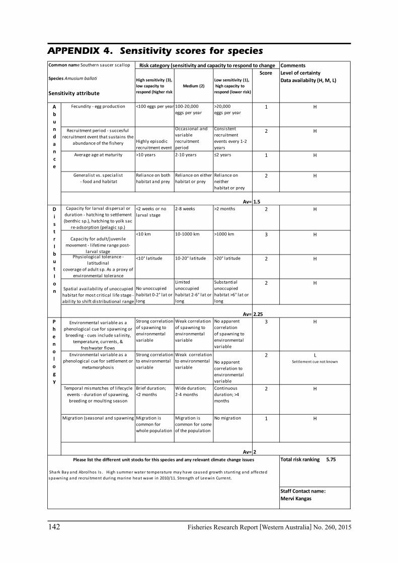
142 Fisheries Research Report [Western Australia] No. 260, 2015
APPENDIX 4. Sensitivity scores for species
<100 eggs per year 100-20,000eggs per year
>20,000eggs per year
1 H
Highly episodicrecruitment event
Occasional and variable recruitment period
Consistentrecruitment events every 1-2 years
2 H
>10 years 2-10 years ≤2 years 1 H
Reliance on bothhabitat and prey
Reliance on eitherhabitat or prey
Reliance on neitherhabitat or prey
2 H
<2 weeks or nolarval stage
2-8 weeks >2 months 2 H
<10 km 10-1000 km >1000 km 3 H
<10° latitude 10-20° latitude >20° latitude 2 H
No unoccupiedhabitat 0-2° lat or long
Limited unoccupiedhabitat 2-6° lat or long
Substantial unoccupiedhabitat >6° lat or long
2 H
Strong correlationof spawning to environmental variable
Weak correlationof spawning to environmental variable
No apparent correlationof spawning to environmental variable
3 H
Strong correlation to environmental variable
Weak correlation to environmental variable
No apparent correlation to environmental variable
2 LSettlement cue not known
Brief duration;<2 months
Wide duration;2-4 months
Continuousduration; >4 months
2 H
Migration is common for whole population
Migration is common for some of the population
No migration 1 H
2.25
1.5
Total risk ranking 5.75
Staff Contact name:Mervi Kangas
Capacity for adult/juvenilemovement - l ifetime range post-
larval stagePhysiological tolerance -
latitudinalcoverage of adult sp. As a proxy of
environmental tolerance
Spatial availabil ity of unoccupiedhabitat for most critical l ife stage - abil ity to shift distributional range
Migration (seasonal and spawning
Please list the different unit stocks for this species and any relevant climate change issues
CommentsLevel of certaintyData availabilty (H, M, L)
Abundance
Av=DistrIbutIon
Av=
Common name Southern saucer scallop
Species Amusium balloti
Sensitivity attribute
Risk category (sensitivity and capacity to respond to change
High sensitivity (3),low capacity to respond (higher risk
Medium (2)Low sensitivity (1), high capacity to respond (lower risk)
Score
Fecundity - egg production
Recruitment period - succesfulrecruitment event that sustains the
abundance of the fishery
Average age at maturity
Generalist vs. specialist - food and habitat
Capacity for larval dispersal orduration - hatching to settlement (benthic sp.), hatching to yolk sac
re-adsorption (pelagic sp.)
Shark Bay and Abrolhos Is . High summer water temperature may have caused growth s tunting and affected spawning and recrui tment during marine heat wave in 2010/11. Strength of Leewin Current.
2
Phenology
Av=
Environmental variable as aphenological cue for spawning or breeding - cues include salinity,
temperature, currents, & freshwater flows
Environmental variable as a phenological cue for settlement or
metamorphosis
Temporal mismatches of l ifecycleevents - duration of spawning, breeding or moulting season
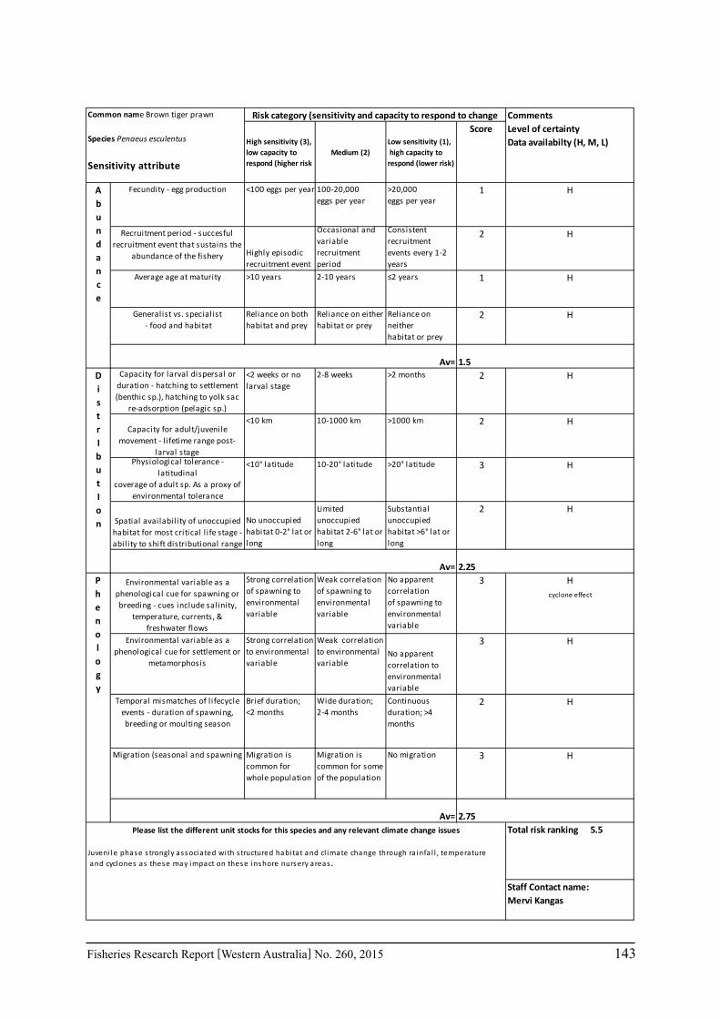
Fisheries Research Report [Western Australia] No. 260, 2015 143
<100 eggs per year 100-20,000eggs per year
>20,000eggs per year
1 H
Highly episodicrecruitment event
Occasional and variable recruitment period
Consistentrecruitment events every 1-2 years
2 H
>10 years 2-10 years ≤2 years 1 H
Reliance on bothhabitat and prey
Reliance on eitherhabitat or prey
Reliance on neitherhabitat or prey
2 H
<2 weeks or nolarval stage
2-8 weeks >2 months 2 H
<10 km 10-1000 km >1000 km 2 H
<10° latitude 10-20° latitude >20° latitude 3 H
No unoccupiedhabitat 0-2° lat or long
Limited unoccupiedhabitat 2-6° lat or long
Substantial unoccupiedhabitat >6° lat or long
2 H
Strong correlationof spawning to environmental variable
Weak correlationof spawning to environmental variable
No apparent correlationof spawning to environmental variable
3 H cyclone effect
Strong correlation to environmental variable
Weak correlation to environmental variable
No apparent correlation to environmental variable
3 H
Brief duration;<2 months
Wide duration;2-4 months
Continuousduration; >4 months
2 H
Migration is common for whole population
Migration is common for some of the population
No migration 3 H
Average age at maturity
Generalist vs. specialist - food and habitat
Av=
Total risk ranking 5.5
Juveni le phase s trongly associated with s tructured habitat and cl imate change through ra infa l l , temperature and cyclones as these may impact on these inshore nursery areas .
Staff Contact name:Mervi Kangas
Phenology
Environmental variable as aphenological cue for spawning or breeding - cues include salinity,
temperature, currents, & freshwater flows
Environmental variable as a phenological cue for settlement or
metamorphosis
Temporal mismatches of l ifecycleevents - duration of spawning, breeding or moulting season
Migration (seasonal and spawning
Av=Please list the different unit stocks for this species and any relevant climate change issues
CommentsLevel of certaintyData availabilty (H, M, L)High sensitivity (3),
low capacity to respond (higher risk
Medium (2)Low sensitivity (1), high capacity to respond (lower risk)
Score
1.5
Abundance
Fecundity - egg production
Recruitment period - succesfulrecruitment event that sustains the
abundance of the fishery
DistrIbutIon
Capacity for larval dispersal orduration - hatching to settlement (benthic sp.), hatching to yolk sac
re-adsorption (pelagic sp.)
Capacity for adult/juvenilemovement - l ifetime range post-
larval stagePhysiological tolerance -
latitudinalcoverage of adult sp. As a proxy of
environmental tolerance
Spatial availabil ity of unoccupiedhabitat for most critical l ife stage - abil ity to shift distributional range
Av= 2.25
2.75
Common name Brown tiger prawn
Species Penaeus esculentus
Sensitivity attribute
Risk category (sensitivity and capacity to respond to change
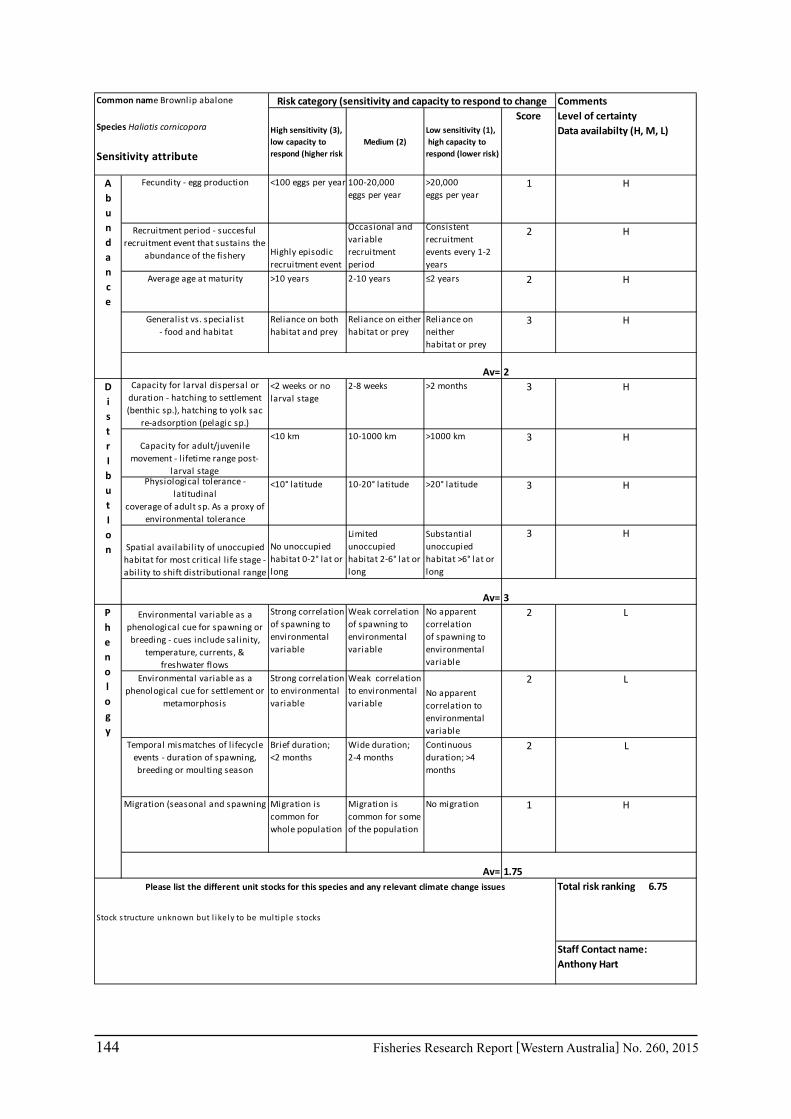
144 Fisheries Research Report [Western Australia] No. 260, 2015
<100 eggs per year 100-20,000eggs per year
>20,000eggs per year
1 H
Highly episodicrecruitment event
Occasional and variable recruitment period
Consistentrecruitment events every 1-2 years
2 H
>10 years 2-10 years ≤2 years 2 H
Reliance on bothhabitat and prey
Reliance on eitherhabitat or prey
Reliance on neitherhabitat or prey
3 H
<2 weeks or nolarval stage
2-8 weeks >2 months 3 H
<10 km 10-1000 km >1000 km 3 H
<10° latitude 10-20° latitude >20° latitude 3 H
No unoccupiedhabitat 0-2° lat or long
Limited unoccupiedhabitat 2-6° lat or long
Substantial unoccupiedhabitat >6° lat or long
3 H
Strong correlationof spawning to environmental variable
Weak correlationof spawning to environmental variable
No apparent correlationof spawning to environmental variable
2 L
Strong correlation to environmental variable
Weak correlation to environmental variable
No apparent correlation to environmental variable
2 L
Brief duration;<2 months
Wide duration;2-4 months
Continuousduration; >4 months
2 L
Migration is common for whole population
Migration is common for some of the population
No migration 1 H
Please list the different unit stocks for this species and any relevant climate change issues
Av=
2DistrIbutIon
Capacity for larval dispersal orduration - hatching to settlement (benthic sp.), hatching to yolk sac
re-adsorption (pelagic sp.)
Capacity for adult/juvenilemovement - l ifetime range post-
larval stagePhysiological tolerance -
latitudinalcoverage of adult sp. As a proxy of
environmental tolerance
Spatial availabil ity of unoccupiedhabitat for most critical l ife stage - abil ity to shift distributional range
Av= 3
Abundance
Fecundity - egg production
Recruitment period - succesfulrecruitment event that sustains the
abundance of the fishery
Average age at maturity
Generalist vs. specialist - food and habitat
Av=
1.75Total risk ranking 6.75
Staff Contact name:Anthony Hart
Stock s tructure unknown but l ikely to be multiple s tocks
Phenology
Environmental variable as aphenological cue for spawning or breeding - cues include salinity,
temperature, currents, & freshwater flows
Environmental variable as a phenological cue for settlement or
metamorphosis
Temporal mismatches of l ifecycleevents - duration of spawning, breeding or moulting season
Migration (seasonal and spawning
Common name Brownlip abalone
Species Haliotis cornicopora
Sensitivity attribute
Risk category (sensitivity and capacity to respond to change CommentsLevel of certaintyData availabilty (H, M, L)High sensitivity (3),
low capacity to respond (higher risk
Medium (2)Low sensitivity (1), high capacity to respond (lower risk)
Score
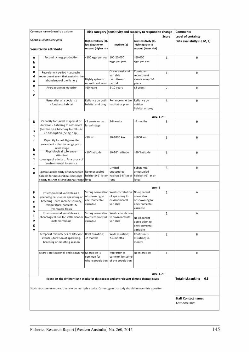
Fisheries Research Report [Western Australia] No. 260, 2015 145
<100 eggs per year 100-20,000eggs per year
>20,000eggs per year
1 H
Highly episodicrecruitment event
Occasional and variable recruitment period
Consistentrecruitment events every 1-2 years
1 H
>10 years 2-10 years ≤2 years 2 H
Reliance on bothhabitat and prey
Reliance on eitherhabitat or prey
Reliance on neitherhabitat or prey
3 H
<2 weeks or nolarval stage
2-8 weeks >2 months 3 H
<10 km 10-1000 km >1000 km 3 H
<10° latitude 10-20° latitude >20° latitude 3 H
No unoccupiedhabitat 0-2° lat or long
Limited unoccupiedhabitat 2-6° lat or long
Substantial unoccupiedhabitat >6° lat or long
3 H
Strong correlationof spawning to environmental variable
Weak correlationof spawning to environmental variable
No apparent correlationof spawning to environmental variable
2 M
Strong correlation to environmental variable
Weak correlation to environmental variable
No apparent correlation to environmental variable
2 M
Brief duration;<2 months
Wide duration;2-4 months
Continuousduration; >4 months
2 H
Migration is common for whole population
Migration is common for some of the population
No migration 1 H
Please list the different unit stocks for this species and any relevant climate change issues
Migration (seasonal and spawning
Av=
1.75DistrIbutIon
Capacity for larval dispersal orduration - hatching to settlement (benthic sp.), hatching to yolk sac
re-adsorption (pelagic sp.)
Capacity for adult/juvenilemovement - l ifetime range post-
larval stagePhysiological tolerance -
latitudinalcoverage of adult sp. As a proxy of
environmental tolerance
Spatial availabil ity of unoccupiedhabitat for most critical l ife stage - abil ity to shift distributional range
Av= 3
Abundance
Fecundity - egg production
Recruitment period - succesfulrecruitment event that sustains the
abundance of the fishery
Average age at maturity
Generalist vs. specialist - food and habitat
Av=
1.75Total risk ranking 6.5
Stock s tructure unknown. Likely to be multiple s tocks . Current genetic s tudy should answer this question
Staff Contact name:Anthony Hart
Phenology
Environmental variable as aphenological cue for spawning or breeding - cues include salinity,
temperature, currents, & freshwater flows
Environmental variable as a phenological cue for settlement or
metamorphosis
Temporal mismatches of l ifecycleevents - duration of spawning, breeding or moulting season
Common name Greenlip abalone
Species Haliotis laevigata
Sensitivity attribute
Risk category (sensitivity and capacity to respond to change CommentsLevel of certaintyData availabilty (H, M, L)High sensitivity (3),
low capacity to respond (higher risk
Medium (2)Low sensitivity (1), high capacity to respond (lower risk)
Score
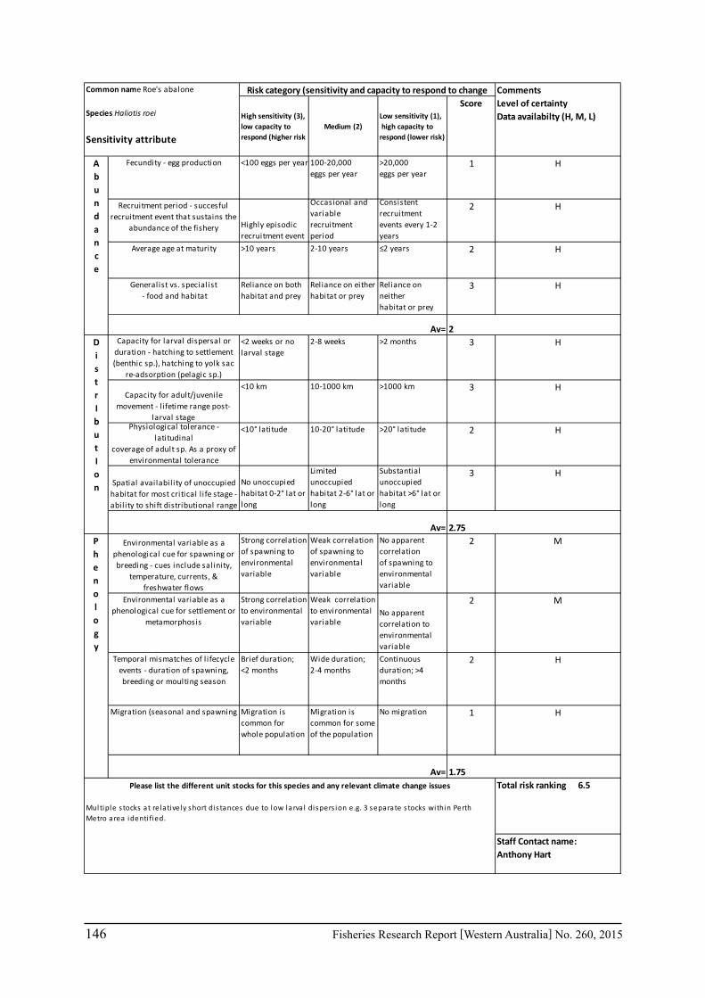
146 Fisheries Research Report [Western Australia] No. 260, 2015
<100 eggs per year 100-20,000eggs per year
>20,000eggs per year
1 H
Highly episodicrecruitment event
Occasional and variable recruitment period
Consistentrecruitment events every 1-2 years
2 H
>10 years 2-10 years ≤2 years 2 H
Reliance on bothhabitat and prey
Reliance on eitherhabitat or prey
Reliance on neitherhabitat or prey
3 H
<2 weeks or nolarval stage
2-8 weeks >2 months 3 H
<10 km 10-1000 km >1000 km 3 H
<10° latitude 10-20° latitude >20° latitude 2 H
No unoccupiedhabitat 0-2° lat or long
Limited unoccupiedhabitat 2-6° lat or long
Substantial unoccupiedhabitat >6° lat or long
3 H
Strong correlationof spawning to environmental variable
Weak correlationof spawning to environmental variable
No apparent correlationof spawning to environmental variable
2 M
Strong correlation to environmental variable
Weak correlation to environmental variable
No apparent correlation to environmental variable
2 M
Brief duration;<2 months
Wide duration;2-4 months
Continuousduration; >4 months
2 H
Migration is common for whole population
Migration is common for some of the population
No migration 1 H
Please list the different unit stocks for this species and any relevant climate change issues
Temporal mismatches of l ifecycleevents - duration of spawning, breeding or moulting season
Migration (seasonal and spawning
Av=
2DistrIbutIon
Capacity for larval dispersal orduration - hatching to settlement (benthic sp.), hatching to yolk sac
re-adsorption (pelagic sp.)
Capacity for adult/juvenilemovement - l ifetime range post-
larval stagePhysiological tolerance -
latitudinalcoverage of adult sp. As a proxy of
environmental tolerance
Spatial availabil ity of unoccupiedhabitat for most critical l ife stage - abil ity to shift distributional range
Av= 2.75
Abundance
Fecundity - egg production
Recruitment period - succesfulrecruitment event that sustains the
abundance of the fishery
Average age at maturity
Generalist vs. specialist - food and habitat
Av=
1.75Total risk ranking 6.5
Multiple s tocks at relatively short dis tances due to low larva l dispers ion e.g. 3 separate s tocks within Perth Metro area identi fied.
Staff Contact name:Anthony Hart
Phenology
Environmental variable as aphenological cue for spawning or breeding - cues include salinity,
temperature, currents, & freshwater flows
Environmental variable as a phenological cue for settlement or
metamorphosis
Common name Roe's abalone
Species Haliotis roei
Sensitivity attribute
Risk category (sensitivity and capacity to respond to change CommentsLevel of certaintyData availabilty (H, M, L)High sensitivity (3),
low capacity to respond (higher risk
Medium (2)Low sensitivity (1), high capacity to respond (lower risk)
Score

Fisheries Research Report [Western Australia] No. 260, 2015 147
<100 eggs per year 100-20,000eggs per year
>20,000eggs per year
1 H
Highly episodicrecruitment event
Occasional and variable recruitment period
Consistentrecruitment events every 1-2 years
2 ?
>10 years 2-10 years ≤2 years 1 H
Reliance on bothhabitat and prey
Reliance on eitherhabitat or prey
Reliance on neitherhabitat or prey
2 H
<2 weeks or nolarval stage
2-8 weeks >2 months 2 H
<10 km 10-1000 km >1000 km 3 H
<10° latitude 10-20° latitude >20° latitude 2 H
No unoccupiedhabitat 0-2° lat or long
Limited unoccupiedhabitat 2-6° lat or long
Substantial unoccupiedhabitat >6° lat or long
2 H
Strong correlationof spawning to environmental variable
Weak correlationof spawning to environmental variable
No apparent correlationof spawning to environmental variable
2 L
Strong correlation to environmental variable
Weak correlation to environmental variable
No apparent correlation to environmental variable
2 L
Brief duration;<2 months
Wide duration;2-4 months
Continuousduration; >4 months
2 L
Migration is common for whole population
Migration is common for some of the population
No migration 1 H
Please list the different unit stocks for this species and any relevant climate change issues
1.75Total risk ranking 5.5
Staff Contact name:Anthony Hart
Phenology
Environmental variable as aphenological cue for spawning or breeding - cues include salinity,
temperature, currents, & freshwater flows
Environmental variable as a phenological cue for settlement or
metamorphosis
Temporal mismatches of l ifecycleevents - duration of spawning, breeding or moulting season
Migration (seasonal and spawning
Av=
1.5DistrIbutIon
Capacity for larval dispersal orduration - hatching to settlement (benthic sp.), hatching to yolk sac
re-adsorption (pelagic sp.)
Capacity for adult/juvenilemovement - l ifetime range post-
larval stagePhysiological tolerance -
latitudinalcoverage of adult sp. As a proxy of
environmental toleranceSpatial availabil ity of unoccupied
habitat for most critical l ife stage - abil ity to shift distributional range
Av= 2.25
Abundance
Fecundity - egg production
Recruitment period - succesfulrecruitment event that sustains the
abundance of the fishery
Average age at maturity
Generalist vs. specialist - food and habitat
Av=
Common name Sandfish (Beche-de-mer)
Species Holothuria scabra
Sensitivity attribute
Risk category (sensitivity and capacity to respond to change CommentsLevel of certaintyData availabilty (H, M, L)High sensitivity (3),
low capacity to respond (higher risk
Medium (2)Low sensitivity (1), high capacity to respond (lower risk)
Score

148 Fisheries Research Report [Western Australia] No. 260, 2015
<100 eggs per year 100-20,000eggs per year
>20,000eggs per year
1 HHighly fecund species - large numbers
of eggs per spawn
Highly episodicrecruitment event
Occasional and variable recruitment period
Consistentrecruitment events every 1-2 years
1 H
>10 years 2-10 years ≤2 years 1 MBased on NT - no research on WA stocks
Reliance on bothhabitat and prey
Reliance on eitherhabitat or prey
Reliance on neitherhabitat or prey
2 HInhabit estuaries and mangroves in
tropical areas
<2 weeks or nolarval stage
2-8 weeks >2 months 2 LNo data specific to WA mud crabs but
assume 2-8 weeks
<10 km 10-1000 km >1000 km 3 H
<10° latitude 10-20° latitude >20° latitude 2 MRestricted to tropical environments of Australia & SE Asia. S. olivacea may be more specific to certain areas as only in large numbers in WA and not Qld &
NT.
No unoccupiedhabitat 0-2° lat or long
Limited unoccupiedhabitat 2-6° lat or long
Substantial unoccupiedhabitat >6° lat or long
2 Not entirely sure but assume all suitable habitat has mud crab
Strong correlationof spawning to environmental variable
Weak correlationof spawning to environmental variable
No apparent correlationof spawning to environmental variable
3 LTemperature (potentially salinity?)
Strong correlation to environmental variable
Weak correlation to environmental variable
No apparent correlation to environmental variable
3 LTemperature (& salinity?)
Brief duration;<2 months
Wide duration;2-4 months
Continuousduration; >4 months
1 LUnsure but assume can spawn over a
number of months as tropical species. May have peak period but no data.
Migration is common for whole population
Migration is common for some of the population
No migration 2 HJuvenile and adults migrate in and out
of estuaries
Av=
1.25DistrIbutIon
Capacity for larval dispersal orduration - hatching to settlement (benthic sp.), hatching to yolk sac
re-adsorption (pelagic sp.)
Capacity for adult/juvenilemovement - l ifetime range post-
larval stagePhysiological tolerance -
latitudinalcoverage of adult sp. As a proxy of
environmental tolerance
Spatial availabil ity of unoccupiedhabitat for most critical l ife stage - abil ity to shift distributional range
Av= 2.25
Abundance
Fecundity - egg production
Recruitment period - succesfulrecruitment event that sustains the
abundance of the fishery
Average age at maturity
Generalist vs. specialist - food and habitat
Av=
2.25Please list the different unit stocks for this species and any relevant climate change issues Total risk ranking 5.75
Very l i ttle known about biology of mud crab in WA. Assume increased water temperature/global warming wi l l be detrimenta l to l i fecycle.
Staff Contact name:Danielle Johnston
Phenology
Environmental variable as aphenological cue for spawning or breeding - cues include salinity,
temperature, currents, & freshwater flows
Environmental variable as a phenological cue for settlement or
metamorphosis
Temporal mismatches of l ifecycleevents - duration of spawning, breeding or moulting season
Migration (seasonal and spawning
Common name Mud Crab
Species Scylla serrata & Scylla olivacea
Sensitivity attribute
Risk category (sensitivity and capacity to respond to change CommentsLevel of certaintyData availabilty (H, M, L)High sensitivity (3),
low capacity to respond (higher risk
Medium (2)Low sensitivity (1), high capacity to respond (lower risk)
Score

Fisheries Research Report [Western Australia] No. 260, 2015 149
<100 eggs per year 100-20,000eggs per year
>20,000eggs per year
1 H
Highly episodicrecruitment event Occasional and
variable recruitment period
Consistentrecruitment events every 1-2 years
1 HSemelparous species with minimal generational overlap, therefore a
failure in recruitment can lead to a population crash
>10 years 2-10 years ≤2 years 1 H
Reliance on bothhabitat and prey
Reliance on eitherhabitat or prey
Reliance on neitherhabitat or prey
1 H
<2 weeks or nolarval stage
2-8 weeks >2 months 1 H
<10 km 10-1000 km >1000 km 2 H
<10° latitude 10-20° latitude >20° latitude 2 H
No unoccupiedhabitat 0-2° lat or long
Limited unoccupiedhabitat 2-6° lat or long
Substantial unoccupiedhabitat >6° lat or long
1 H
Strong correlationof spawning to environmental variable
Weak correlationof spawning to environmental variable
No apparent correlationof spawning to environmental variable
3 HTemperature
Strong correlation to environmental variable
Weak correlation to environmental variable
No apparent correlation to environmental variable
3 HTemperature
Brief duration;<2 months
Wide duration;2-4 months
Continuousduration; >4 months
2 H
Migration is common for whole population
Migration is common for some of the population
No migration 1 MMovement patterns not determined.
Potential small scale movements between inshore and offshore.
Temporal mismatches of l ifecycleevents - duration of spawning, breeding or moulting season
Migration (seasonal and spawning
Av=
1DistrIbutIon
Capacity for larval dispersal orduration - hatching to settlement (benthic sp.), hatching to yolk sac
re-adsorption (pelagic sp.)
Capacity for adult/juvenilemovement - l ifetime range post-
larval stagePhysiological tolerance -
latitudinalcoverage of adult sp. As a proxy of
environmental tolerance
Spatial availabil ity of unoccupiedhabitat for most critical l ife stage - abil ity to shift distributional range
Av= 1.5
Abundance
Fecundity - egg production
Recruitment period - succesfulrecruitment event that sustains the
abundance of the fishery
Average age at maturity
Generalist vs. specialist - food and habitat
Av=
2.25Please list the different unit stocks for this species and any relevant climate change issues Total risk ranking 4.75
Two potentia l populations . One on the west coast from Shark Bay to cape Leeuwin, and another on the south coast to the SA border.
Staff Contact name:Stephen Leporati
Erratic envi ronmenta l changes may lead to digni fican short term changes to the dynamics of these fast growing, shortly l ived, highly fecund animals .
As ecologica l opportunis ts cl imate change may prove beneficia l , however ocean acidi fication may prove harmful at the para larva l s tage.
Phenology
Environmental variable as aphenological cue for spawning or breeding - cues include salinity,
temperature, currents, & freshwater flows
Environmental variable as a phenological cue for settlement or
metamorphosis
Common name Gloomy Octopus
Species Octopus tetricus
Sensitivity attribute
Risk category (sensitivity and capacity to respond to change CommentsLevel of certaintyData availabilty (H, M, L)High sensitivity (3),
low capacity to respond (higher risk
Medium (2)Low sensitivity (1), high capacity to respond (lower risk)
Score

150 Fisheries Research Report [Western Australia] No. 260, 2015
<100 eggs per year 100-20,000eggs per year
>20,000eggs per year
1 H
Highly episodicrecruitment event Occasional and
variable recruitment period
Consistentrecruitment events every 1-2 years
2 H
>10 years 2-10 years ≤2 years 2 H
Reliance on bothhabitat and prey
Reliance on eitherhabitat or prey
Reliance on neitherhabitat or prey
2 H
<2 weeks or nolarval stage
2-8 weeks >2 months 1 H
<10 km 10-1000 km >1000 km 2 H
<10° latitude 10-20° latitude >20° latitude 2 H
No unoccupiedhabitat 0-2° lat or long
Limited unoccupiedhabitat 2-6° lat or long
Substantial unoccupiedhabitat >6° lat or long
2 H
Strong correlationof spawning to environmental variable
Weak correlationof spawning to environmental variable
No apparent correlationof spawning to environmental variable
3 H
Strong correlation to environmental variable
Weak correlation to environmental variable
No apparent correlation to environmental variable
3 H
Brief duration;<2 months
Wide duration;2-4 months
Continuousduration; >4 months
2 HMismatch between the spawning
period and the larval phase may be possible cause of last 7 years of low
puerulus settlement.
Migration is common for whole population
Migration is common for some of the population
No migration 3 H
2.75
Please list the different unit stocks for this species and any relevant climate change issues Total risk ranking 6.25Effects of increas ing water temperature has been shown to affect s i ze of migration and s ize at maturi ty (Caputi et a l . 2010). Recent s tudies have identi fied a poss ible mismatch between the spawning period and the larva l phase as the poss ible cause of las t 7 years of low puerulus settlement. The increas ing water temperature at the time of spawning appears to have moved the spawning period forward.
Staff Contact name:Nick Caputi
Phenology
Environmental variable as aphenological cue for spawning or breeding - cues include salinity,
temperature, currents, & freshwater flows
Environmental variable as a phenological cue for settlement or
metamorphosis
Temporal mismatches of l ifecycleevents - duration of spawning, breeding or moulting season
Migration (seasonal and spawning
Av=
1.75DistrIbutIon
Capacity for larval dispersal orduration - hatching to settlement (benthic sp.), hatching to yolk sac
re-adsorption (pelagic sp.)
Capacity for adult/juvenilemovement - l ifetime range post-
larval stagePhysiological tolerance -
latitudinalcoverage of adult sp. As a proxy of
environmental tolerance
Spatial availabil ity of unoccupiedhabitat for most critical l ife stage - abil ity to shift distributional range
Av= 1.5
Abundance
Fecundity - egg production
Recruitment period - succesfulrecruitment event that sustains the
abundance of the fishery
Average age at maturity
Generalist vs. specialist - food and habitat
Av=
Common name Western rock lobster
Species Panulirus cygnus
Sensitivity attribute
Risk category (sensitivity and capacity to respond to change CommentsLevel of certaintyData availabilty (H, M, L)High sensitivity (3),
low capacity to respond (higher risk
Medium (2)Low sensitivity (1), high capacity to respond (lower risk)
Score

Fisheries Research Report [Western Australia] No. 260, 2015 151
<100 eggs per year 100-20,000eggs per year
>20,000eggs per year
1 H
Highly episodicrecruitment event Occasional and
variable recruitment period
Consistentrecruitment events every 1-2 years
2 H
>10 years 2-10 years ≤2 years 2 H
Reliance on bothhabitat and prey
Reliance on eitherhabitat or prey
Reliance on neitherhabitat or prey
2 H
<2 weeks or nolarval stage
2-8 weeks >2 months 2 H
<10 km 10-1000 km >1000 km 3 H
<10° latitude 10-20° latitude >20° latitude 2 H
No unoccupiedhabitat 0-2° lat or long
Limited unoccupiedhabitat 2-6° lat or long
Substantial unoccupiedhabitat >6° lat or long
2 H
Strong correlationof spawning to environmental variable
Weak correlationof spawning to environmental variable
No apparent correlationof spawning to environmental variable
3 H
Strong correlation to environmental variable
Weak correlation to environmental variable
No apparent correlation to environmental variable
3 H
Brief duration;<2 months
Wide duration;2-4 months
Continuousduration; >4 months
2 H
Migration is common for whole population
Migration is common for some of the population
No migration 1 HMigration (seasonal and spawning
Av=
1.75DistrIbutIon
Capacity for larval dispersal orduration - hatching to settlement (benthic sp.), hatching to yolk sac
re-adsorption (pelagic sp.)
Capacity for adult/juvenilemovement - l ifetime range post-
larval stagePhysiological tolerance -
latitudinalcoverage of adult sp. As a proxy of
environmental tolerance
Spatial availabil ity of unoccupiedhabitat for most critical l ife stage - abil ity to shift distributional range
Av= 2.25
Abundance
Fecundity - egg production
Recruitment period - succesfulrecruitment event that sustains the
abundance of the fishery
Average age at maturity
Generalist vs. specialist - food and habitat
Av=
2.25Please list the different unit stocks for this species and any relevant climate change issues Total risk ranking 6.25
Exmouth Gul f, 80 Mi le Beach
Environmenta l factors (water temperature, wind and cyclones) a ffecting recrui tment at 80 Mi le Beach have been identi fied.
Staff Contact name:Anthony Hart
Phenology
Environmental variable as aphenological cue for spawning or breeding - cues include salinity,
temperature, currents, & freshwater flows
Environmental variable as a phenological cue for settlement or
metamorphosis
Temporal mismatches of l ifecycleevents - duration of spawning, breeding or moulting season
Common name Silver l ipped pearl oyster
Species Pinctada maxima
Sensitivity attribute
Risk category (sensitivity and capacity to respond to change CommentsLevel of certaintyData availabilty (H, M, L)High sensitivity (3),
low capacity to respond (higher risk
Medium (2)Low sensitivity (1), high capacity to respond (lower risk)
Score

152 Fisheries Research Report [Western Australia] No. 260, 2015
<100 eggs per year 100-20,000eggs per year
>20,000eggs per year
1 HLarge numbers of eggs per spawning, 0.6-1.2 million eggs per spawning
(Kumar et al, 2000)
Highly episodicrecruitment event Occasional and
variable recruitment period
Consistentrecruitment events every 1-2 years
1 HRecruitment consistent but can be variable between years on account of environmental conditions, e.g. temperature in southwest affects recruitment
>10 years 2-10 years ≤2 years 1 HSize at maturity attained generally within 12 months. Potentially faster in Shark Bay
Reliance on bothhabitat and prey
Reliance on eitherhabitat or prey
Reliance on neitherhabitat or prey
2 HBSC inhabit wide range of habitats inshore. However prefer seagrass/algal habitats particularly during recruitment for nursery grounds
<2 weeks or nolarval stage
2-8 weeks >2 months 2 H
<10 km 10-1000 km >1000 km 3 H
<10° latitude 10-20° latitude >20° latitude 1 HExtends form ~Nickol Bay (Pilbara) to S of Mandurah. Fisheries in SW are more sensitive to environmental conditions of temperature as at extreme of range
for tropical species
No unoccupiedhabitat 0-2° lat or long
Limited unoccupiedhabitat 2-6° lat or long
Substantial unoccupiedhabitat >6° lat or long
2 Inhabit all areas of WA coast that have suitable habitat and environmental
conditions
Strong correlationof spawning to environmental variable
Weak correlationof spawning to environmental variable
No apparent correlationof spawning to environmental variable
3 HTemperature
Strong correlation to environmental variable
Weak correlation to environmental variable
No apparent correlation to environmental variable
3 HTemperature
Brief duration;<2 months
Wide duration;2-4 months
Continuousduration; >4 months
2 HSouthern fisheries Sept-Dec/Jan; Shark
Bay & northern fisheries continuous but potential peak Jul-Sept
Migration is common for whole population
Migration is common for some of the population
No migration 2 Juvenile migrate into PH estuary and also adults/subadults migrate to
deeper waters - females move out of estuary to spawn. May have limited
migration between SW fisheries
Environmental variable as a phenological cue for settlement or
metamorphosis
Temporal mismatches of l ifecycleevents - duration of spawning, breeding or moulting season
Migration (seasonal and spawning
Av=
1.25DistrIbutIon
Capacity for larval dispersal orduration - hatching to settlement (benthic sp.), hatching to yolk sac
re-adsorption (pelagic sp.)Capacity for adult/juvenile
movement - l ifetime range post-larval stage
Physiological tolerance - latitudinal
coverage of adult sp. As a proxy of environmental tolerance
Spatial availabil ity of unoccupiedhabitat for most critical l ife stage - abil ity to shift distributional range
Av= 2
Abundance
Fecundity - egg production
Recruitment period - succesfulrecruitment event that sustains the
abundance of the fishery
Average age at maturity
Generalist vs. specialist - food and habitat
Av=
2.25Please list the different unit stocks for this species and any relevant climate change issues 5.75
Nickol Bay & Shark Bay at ri sk of cl imate change i f temps increase. Shark Bay s tock s igni ficantly affected by marine heat wave of 2010/11.
SW (Cockburn Sound, Swan River, Peel harvey Estuary, Warnbro Sound, Mandurah-Bunbury & Comet Bay, Leschenault) highly sens i tive to environementa l changes particularly temperature at extreme of geographic range for tropica l species . Recrui tment success , spawning success and growth rel iant on temperature. Warming of water temperatures may benefi t recrui tment/spawning/growth in these fi sheries .
Staff Contact name:Danielle Johnston
Phenology
Environmental variable as aphenological cue for spawning or breeding - cues include salinity,
temperature, currents, & freshwater flows
Common name Blue Swimmer Crab
Species Portunus armatus (pelagicus)
Sensitivity attribute
Risk category (sensitivity and capacity to respond to change CommentsLevel of certaintyData availabilty (H, M, L)High sensitivity (3),
low capacity to respond (higher risk
Medium (2)Low sensitivity (1), high capacity to respond (lower risk)
Score

Fisheries Research Report [Western Australia] No. 260, 2015 153
<100 eggs per year 100-20,000eggs per year
>20,000eggs per year
1 H
Highly episodicrecruitment event Occasional and
variable recruitment period
Consistentrecruitment events every 1-2 years
2 H
>10 years 2-10 years ≤2 years 1 H
Reliance on bothhabitat and prey
Reliance on eitherhabitat or prey
Reliance on neitherhabitat or prey
2 H
<2 weeks or nolarval stage
2-8 weeks >2 months 2 H
<10 km 10-1000 km >1000 km 2 M
<10° latitude 10-20° latitude >20° latitude 2 H
No unoccupiedhabitat 0-2° lat or long
Limited unoccupiedhabitat 2-6° lat or long
Substantial unoccupiedhabitat >6° lat or long
2 M
Strong correlationof spawning to environmental variable
Weak correlationof spawning to environmental variable
No apparent correlationof spawning to environmental variable
2 M
Strong correlation to environmental variable
Weak correlation to environmental variable
No apparent correlation to environmental variable
3 H
Brief duration;<2 months
Wide duration;2-4 months
Continuousduration; >4 months
1 H
Migration is common for whole population
Migration is common for some of the population
No migration 3 H
2.25Please list the different unit stocks for this species and any relevant climate change issues Total risk ranking 5.375
Northern extens ion of range may be impacted by warmmer water temperatures with resul ting lower abundance. Higher ra infa l l events and reduced sa l ini ty could impact on dis tribution of juveni le prawns .
Phenology
Environmental variable as aphenological cue for spawning or breeding - cues include salinity,
temperature, currents, & freshwater flows
Environmental variable as a phenological cue for settlement or
metamorphosis
Temporal mismatches of l ifecycleevents - duration of spawning, breeding or moulting season
Migration (seasonal and spawning
Av=
Staff Contact name:Mervi Kangas
1.5DistrIbutIon
Capacity for larval dispersal orduration - hatching to settlement (benthic sp.), hatching to yolk sac
re-adsorption (pelagic sp.)Capacity for adult/juvenile
movement - l ifetime range post-larval stage
Physiological tolerance - latitudinal
coverage of adult sp. As a proxy of environmental tolerance
Spatial availabil ity of unoccupiedhabitat for most critical l ife stage - abil ity to shift distributional range
Av= 2
Abundance
Fecundity - egg production
Recruitment period - succesfulrecruitment event that sustains the
abundance of the fishery
Average age at maturity
Generalist vs. specialist - food and habitat
Av=
Common name Western king prawn
Species Penaeus latisulcatus
Sensitivity attribute
Risk category (sensitivity and capacity to respond to change CommentsLevel of certaintyData availabilty (H, M, L)High sensitivity (3),
low capacity to respond (higher risk
Medium (2)Low sensitivity (1), high capacity to respond (lower risk)
Score

154 Fisheries Research Report [Western Australia] No. 260, 2015
<100 eggs per year 100-20,000eggs per year
>20,000eggs per year
1 H
Highly episodicrecruitment event Occasional and
variable recruitment period
Consistentrecruitment events every 1-2 years
2 H
>10 years 2-10 years ≤2 years 2 H
Reliance on bothhabitat and prey
Reliance on eitherhabitat or prey
Reliance on neitherhabitat or prey
2 M
<2 weeks or nolarval stage
2-8 weeks >2 months 2 H
<10 km 10-1000 km >1000 km 1 H
<10° latitude 10-20° latitude >20° latitude 2 H
No unoccupiedhabitat 0-2° lat or long
Limited unoccupiedhabitat 2-6° lat or long
Substantial unoccupiedhabitat >6° lat or long
2 H
Strong correlationof spawning to environmental variable
Weak correlationof spawning to environmental variable
No apparent correlationof spawning to environmental variable
3 H
Strong correlation to environmental variable
Weak correlation to environmental variable
No apparent correlation to environmental variable
2 H
Brief duration;<2 months
Wide duration;2-4 months
Continuousduration; >4 months
3 H
Migration is common for whole population
Migration is common for some of the population
No migration 3 H(for most of the population)
Dis tribution of larvae/smal l juveni les to south coast nursery areas dependent on s trength of Leeuwin Current.Staff Contact name:Kim SmithJosh Brown
Recrui tment from south coast population to west coast fi shable s tock dependent on Leeuwin Current s trength and SST.
Phenology
Environmental variable as aphenological cue for spawning or breeding - cues include salinity,
temperature, currents, & freshwater flows
Environmental variable as a phenological cue for settlement or
metamorphosis
Temporal mismatches of l ifecycleevents - duration of spawning, breeding or moulting season
Migration (seasonal and spawning
Av=
1.75DistrIbutIon
Capacity for larval dispersal orduration - hatching to settlement (benthic sp.), hatching to yolk sac
re-adsorption (pelagic sp.)Capacity for adult/juvenile
movement - l ifetime range post-larval stage
Physiological tolerance - latitudinal
coverage of adult sp. As a proxy of environmental tolerance
Spatial availabil ity of unoccupiedhabitat for most critical l ife stage - abil ity to shift distributional range
Av= 1.75
Abundance
Fecundity - egg production
Recruitment period - succesfulrecruitment event that sustains the
abundance of the fishery
Average age at maturity
Generalist vs. specialist - food and habitat
Av=
2.5Please list the different unit stocks for this species and any relevant climate change issues Total risk ranking 6.0
West and south coast 'management uni ts ' recognized.
Common name Australian Herring
Species Arripis georgianus
Sensitivity attribute
Risk category (sensitivity and capacity to respond to change CommentsLevel of certaintyData availabilty (H, M, L)High sensitivity (3),
low capacity to respond (higher risk
Medium (2)Low sensitivity (1), high capacity to respond (lower risk)
Score

Fisheries Research Report [Western Australia] No. 260, 2015 155
<100 eggs per year 100-20,000eggs per year
>20,000eggs per year
1 H
Highly episodicrecruitment event Occasional and
variable recruitment period
Consistentrecruitment events every 1-2 years
3 H
>10 years 2-10 years ≤2 years 2 H
Reliance on bothhabitat and prey
Reliance on eitherhabitat or prey
Reliance on neitherhabitat or prey
1 H
<2 weeks or nolarval stage
2-8 weeks >2 months 3 H
<10 km 10-1000 km >1000 km 3 H(don't genearlly move between
estuaries, hence '3')
<10° latitude 10-20° latitude >20° latitude 3 H
No unoccupiedhabitat 0-2° lat or long
Limited unoccupiedhabitat 2-6° lat or long
Substantial unoccupiedhabitat >6° lat or long
3 H
Strong correlationof spawning to environmental variable
Weak correlationof spawning to environmental variable
No apparent correlationof spawning to environmental variable
3 H
Strong correlation to environmental variable
Weak correlation to environmental variable
No apparent correlation to environmental variable
2 L
Brief duration;<2 months
Wide duration;2-4 months
Continuousduration; >4 months
2 H
Migration is common for whole population
Migration is common for some of the population
No migration 1 H
Common name Black Bream
Species Acanthopagrus butcherii
Sensitivity attribute
Risk category (sensitivity and capacity to respond to change CommentsLevel of certaintyData availabilty (H, M, L)High sensitivity (3),
low capacity to respond (higher risk
Medium (2)Low sensitivity (1), high capacity to respond (lower risk)
Score
Abundance
Fecundity - egg production
Recruitment period - succesfulrecruitment event that sustains the
abundance of the fishery
Average age at maturity
Generalist vs. specialist - food and habitat
Av= 1.75
Please list the different unit stocks for this species and any relevant climate change issues Total risk ranking 6.75
Discrete, breeding s tock in each estuary. Found in most estuaries across range.
Widespread dis tribution = temperate zones of WA, SA, Vic & southern NSW. Warmer temperatures and reduced ra infa l l wi l l cause a contraction of the range.
Staff Contact name:Kim Smith
DistrIbutIon
Capacity for larval dispersal orduration - hatching to settlement (benthic sp.), hatching to yolk sac
re-adsorption (pelagic sp.)Capacity for adult/juvenile
movement - l ifetime range post-larval stage
Physiological tolerance - latitudinal
coverage of adult sp. As a proxy of environmental tolerance
Spatial availabil ity of unoccupiedhabitat for most critical l ife stage - abil ity to shift distributional range
Av= 3Phenology
Environmental variable as aphenological cue for spawning or breeding - cues include salinity,
temperature, currents, & freshwater flows
Environmental variable as a phenological cue for settlement or
metamorphosis
Temporal mismatches of l ifecycleevents - duration of spawning, breeding or moulting season
Migration (seasonal and spawning
Av= 2

156 Fisheries Research Report [Western Australia] No. 260, 2015
<100 eggs per year 100-20,000eggs per year
>20,000eggs per year
1 M
Highly episodicrecruitment event Occasional and
variable recruitment period
Consistentrecruitment events every 1-2 years
2 M
>10 years 2-10 years ≤2 years 1 Mbased on when female is mature
Reliance on bothhabitat and prey
Reliance on eitherhabitat or prey
Reliance on neitherhabitat or prey
2 L
<2 weeks or nolarval stage
2-8 weeks >2 months 2 L
<10 km 10-1000 km >1000 km 3 L
<10° latitude 10-20° latitude >20° latitude 3 M
No unoccupiedhabitat 0-2° lat or long
Limited unoccupiedhabitat 2-6° lat or long
Substantial unoccupiedhabitat >6° lat or long
2 H
Strong correlationof spawning to environmental variable
Weak correlationof spawning to environmental variable
No apparent correlationof spawning to environmental variable
2 H
Strong correlation to environmental variable
Weak correlation to environmental variable
No apparent correlation to environmental variable
2 L
Brief duration;<2 months
Wide duration;2-4 months
Continuousduration; >4 months
2 H
Migration is common for whole population
Migration is common for some of the population
No migration 1 L
Common name Blue threadfin
Species Eleutheronema tetradactylum
Sensitivity attribute
Risk category (sensitivity and capacity to respond to change CommentsLevel of certaintyData availabilty (H, M, L)High sensitivity (3),
low capacity to respond (higher risk
Medium (2)Low sensitivity (1), high capacity to respond (lower risk)
Score
Phenology
Environmental variable as aphenological cue for spawning or breeding - cues include salinity,
temperature, currents, & freshwater flows
Environmental variable as a phenological cue for settlement or
metamorphosis
Temporal mismatches of l ifecycleevents - duration of spawning, breeding or moulting season
Migration (seasonal and spawning
Av= 1.75Please list the different unit stocks for this species and any relevant climate change issues Total risk ranking 5.75
Evidence of separate genetic s tocks , and multiple separate adult management uni ts l ikely (adults have l imited movements , dispersa l )
Abundance
Fecundity - egg production
Recruitment period - succesfulrecruitment event that sustains the
abundance of the fishery
Average age at maturity
Generalist vs. specialist - food and habitat
Av= 1.5DistrIbutIon
Capacity for larval dispersal orduration - hatching to settlement (benthic sp.), hatching to yolk sac
re-adsorption (pelagic sp.)Capacity for adult/juvenile
movement - l ifetime range post-larval stage
Physiological tolerance - latitudinal
coverage of adult sp. As a proxy of environmental tolerance
Spatial availabil ity of unoccupiedhabitat for most critical l ife stage - abil ity to shift distributional range
Av= 2.5
Staff Contact name:Stephen Newman
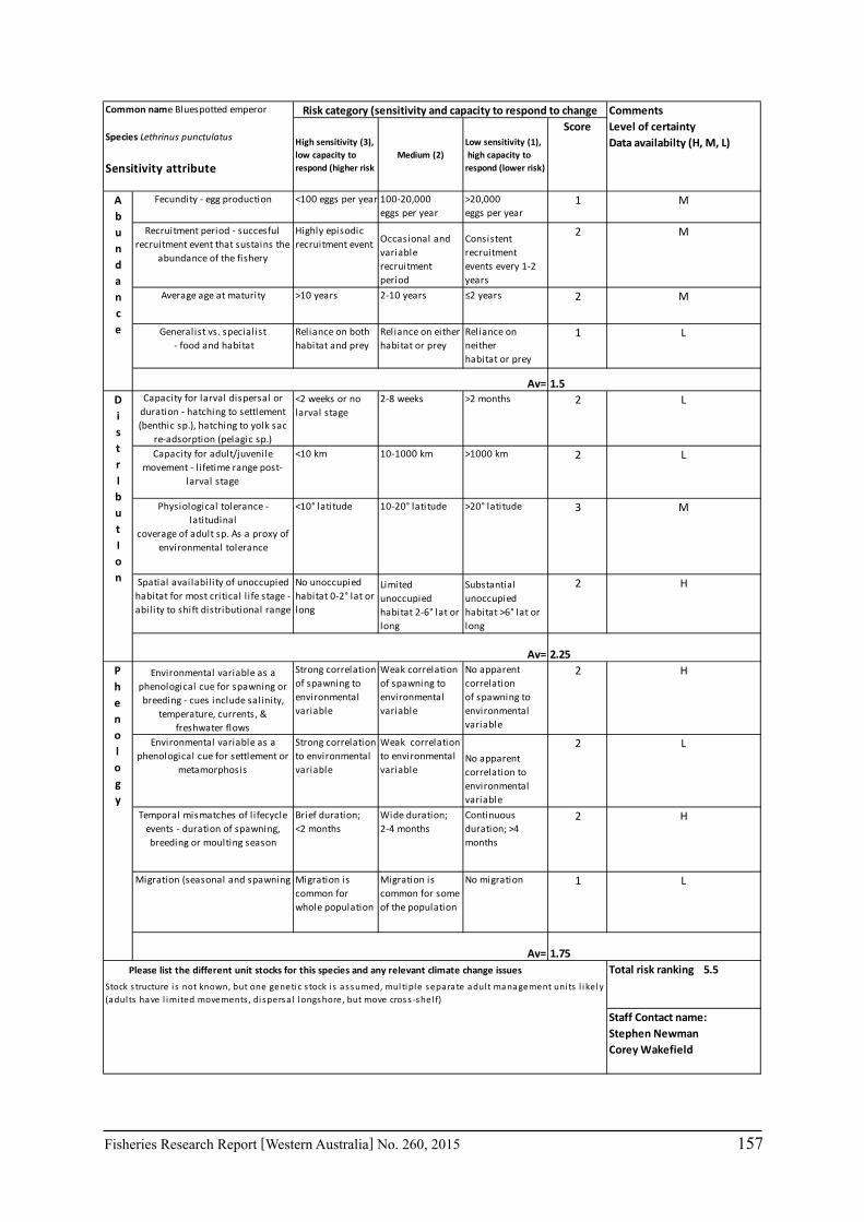
Fisheries Research Report [Western Australia] No. 260, 2015 157
<100 eggs per year 100-20,000eggs per year
>20,000eggs per year
1 M
Highly episodicrecruitment event Occasional and
variable recruitment period
Consistentrecruitment events every 1-2 years
2 M
>10 years 2-10 years ≤2 years 2 M
Reliance on bothhabitat and prey
Reliance on eitherhabitat or prey
Reliance on neitherhabitat or prey
1 L
<2 weeks or nolarval stage
2-8 weeks >2 months 2 L
<10 km 10-1000 km >1000 km 2 L
<10° latitude 10-20° latitude >20° latitude 3 M
No unoccupiedhabitat 0-2° lat or long
Limited unoccupiedhabitat 2-6° lat or long
Substantial unoccupiedhabitat >6° lat or long
2 H
Strong correlationof spawning to environmental variable
Weak correlationof spawning to environmental variable
No apparent correlationof spawning to environmental variable
2 H
Strong correlation to environmental variable
Weak correlation to environmental variable
No apparent correlation to environmental variable
2 L
Brief duration;<2 months
Wide duration;2-4 months
Continuousduration; >4 months
2 H
Migration is common for whole population
Migration is common for some of the population
No migration 1 L
Abundance
Fecundity - egg production
Recruitment period - succesfulrecruitment event that sustains the
abundance of the fishery
Average age at maturity
Generalist vs. specialist - food and habitat
Av= 1.5DistrIbutIon
Capacity for larval dispersal orduration - hatching to settlement (benthic sp.), hatching to yolk sac
re-adsorption (pelagic sp.)Capacity for adult/juvenile
movement - l ifetime range post-larval stage
Physiological tolerance - latitudinal
coverage of adult sp. As a proxy of environmental tolerance
Spatial availabil ity of unoccupiedhabitat for most critical l ife stage - abil ity to shift distributional range
Av= 2.25
Common name Bluespotted emperor
Species Lethrinus punctulatus
Sensitivity attribute
Risk category (sensitivity and capacity to respond to change CommentsLevel of certaintyData availabilty (H, M, L)High sensitivity (3),
low capacity to respond (higher risk
Medium (2)Low sensitivity (1), high capacity to respond (lower risk)
Score
Staff Contact name:Stephen NewmanCorey Wakefield
Phenology
Environmental variable as aphenological cue for spawning or breeding - cues include salinity,
temperature, currents, & freshwater flows
Environmental variable as a phenological cue for settlement or
metamorphosis
Temporal mismatches of l ifecycleevents - duration of spawning, breeding or moulting season
Migration (seasonal and spawning
Av= 1.75Please list the different unit stocks for this species and any relevant climate change issues Total risk ranking 5.5
Stock s tructure i s not known, but one genetic s tock i s assumed, multiple separate adult management uni ts l ikely (adul ts have l imited movements , dispersa l longshore, but move cross -shel f)
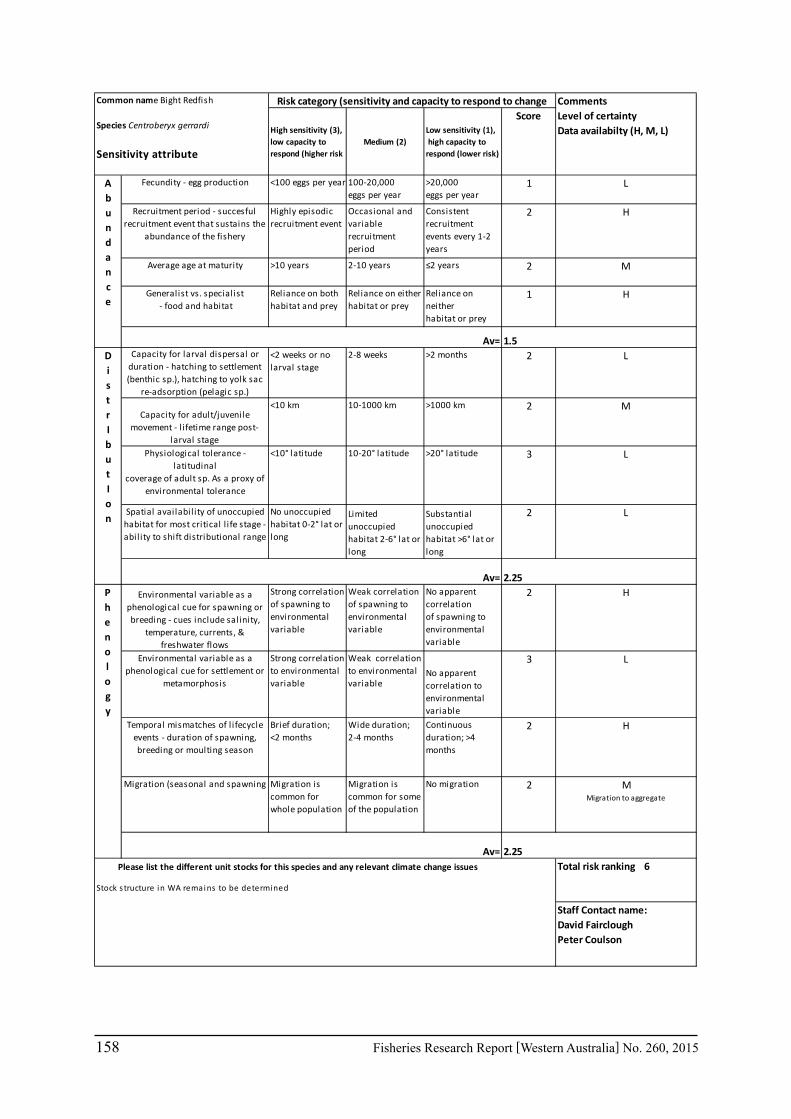
158 Fisheries Research Report [Western Australia] No. 260, 2015
<100 eggs per year 100-20,000eggs per year
>20,000eggs per year
1 L
Highly episodicrecruitment event
Occasional and variable recruitment period
Consistentrecruitment events every 1-2 years
2 H
>10 years 2-10 years ≤2 years 2 M
Reliance on bothhabitat and prey
Reliance on eitherhabitat or prey
Reliance on neitherhabitat or prey
1 H
<2 weeks or nolarval stage
2-8 weeks >2 months 2 L
<10 km 10-1000 km >1000 km 2 M
<10° latitude 10-20° latitude >20° latitude 3 L
No unoccupiedhabitat 0-2° lat or long
Limited unoccupiedhabitat 2-6° lat or long
Substantial unoccupiedhabitat >6° lat or long
2 L
Strong correlationof spawning to environmental variable
Weak correlationof spawning to environmental variable
No apparent correlationof spawning to environmental variable
2 H
Strong correlation to environmental variable
Weak correlation to environmental variable
No apparent correlation to environmental variable
3 L
Brief duration;<2 months
Wide duration;2-4 months
Continuousduration; >4 months
2 H
Migration is common for whole population
Migration is common for some of the population
No migration 2 MMigration to aggregate
Common name Bight Redfish
Species Centroberyx gerrardi
Sensitivity attribute
Risk category (sensitivity and capacity to respond to change CommentsLevel of certaintyData availabilty (H, M, L)High sensitivity (3),
low capacity to respond (higher risk
Medium (2)Low sensitivity (1), high capacity to respond (lower risk)
Score
Phenology
Environmental variable as aphenological cue for spawning or breeding - cues include salinity,
temperature, currents, & freshwater flows
Environmental variable as a phenological cue for settlement or
metamorphosis
Temporal mismatches of l ifecycleevents - duration of spawning, breeding or moulting season
Migration (seasonal and spawning
Av= 2.25Please list the different unit stocks for this species and any relevant climate change issues Total risk ranking 6
Stock s tructure in WA remains to be determined
Abundance
Fecundity - egg production
Recruitment period - succesfulrecruitment event that sustains the
abundance of the fishery
Average age at maturity
Generalist vs. specialist - food and habitat
Av= 1.5DistrIbutIon
Capacity for larval dispersal orduration - hatching to settlement (benthic sp.), hatching to yolk sac
re-adsorption (pelagic sp.)
Capacity for adult/juvenilemovement - l ifetime range post-
larval stagePhysiological tolerance -
latitudinalcoverage of adult sp. As a proxy of
environmental tolerance
Spatial availabil ity of unoccupiedhabitat for most critical l ife stage - abil ity to shift distributional range
Av= 2.25
Staff Contact name:David FaircloughPeter Coulson

Fisheries Research Report [Western Australia] No. 260, 2015 159
<100 eggs per year 100-20,000eggs per year
>20,000eggs per year
1 H
Highly episodicrecruitment event
Occasional and variable recruitment period
Consistentrecruitment events every 1-2 years
2 H
>10 years 2-10 years ≤2 years 2 Hplus protogynous sex change
Reliance on bothhabitat and prey
Reliance on eitherhabitat or prey
Reliance on neitherhabitat or prey
2 H(habitat reliance)
<2 weeks or nolarval stage
2-8 weeks >2 months 2 M
<10 km 10-1000 km >1000 km 3 H
<10° latitude 10-20° latitude >20° latitude 2 H
No unoccupiedhabitat 0-2° lat or long
Limited unoccupiedhabitat 2-6° lat or long
Substantial unoccupiedhabitat >6° lat or long
2 H
Strong correlationof spawning to environmental variable
Weak correlationof spawning to environmental variable
No apparent correlationof spawning to environmental variable
3 H
Strong correlation to environmental variable
Weak correlation to environmental variable
No apparent correlation to environmental variable
1 L
Brief duration;<2 months
Wide duration;2-4 months
Continuousduration; >4 months
2 H
Migration is common for whole population
Migration is common for some of the population
No migration 1 H
Abundance
Fecundity - egg production
Recruitment period - succesfulrecruitment event that sustains the
abundance of the fishery
Average age at maturity
Generalist vs. specialist - food and habitat
Av= 1.75DistrIbutIon
Capacity for larval dispersal orduration - hatching to settlement (benthic sp.), hatching to yolk sac
re-adsorption (pelagic sp.)
Capacity for adult/juvenilemovement - l ifetime range post-
larval stagePhysiological tolerance -
latitudinalcoverage of adult sp. As a proxy of
environmental tolerance
Spatial availabil ity of unoccupiedhabitat for most critical l ife stage - abil ity to shift distributional range
Av= 2.25
Common name Baldchin groper
Species Choerodon rubescens
Sensitivity attribute
Risk category (sensitivity and capacity to respond to change CommentsLevel of certaintyData availabilty (H, M, L)High sensitivity (3),
low capacity to respond (higher risk
Medium (2)Low sensitivity (1), high capacity to respond (lower risk)
Score
Staff Contact name:David Fairclough
Phenology
Environmental variable as aphenological cue for spawning or breeding - cues include salinity,
temperature, currents, & freshwater flows
Environmental variable as a phenological cue for settlement or
metamorphosis
Temporal mismatches of l ifecycleevents - duration of spawning, breeding or moulting season
Migration (seasonal and spawning
Av= 1.75Please list the different unit stocks for this species and any relevant climate change issues Total risk ranking 5.75
Currently "fi shable s tocks" are bioregional -based (i .e. South coast, West coast, Gascoyne). However resul ts of ongoing research may change this .
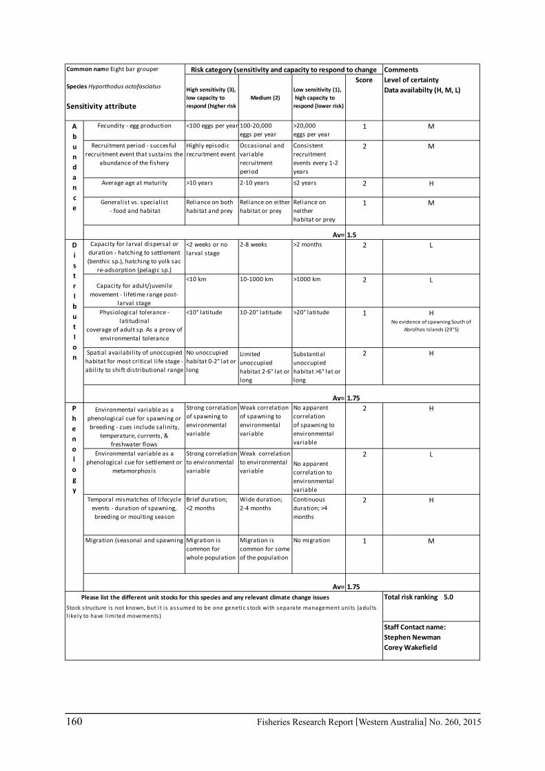
160 Fisheries Research Report [Western Australia] No. 260, 2015
<100 eggs per year 100-20,000eggs per year
>20,000eggs per year
1 M
Highly episodicrecruitment event
Occasional and variable recruitment period
Consistentrecruitment events every 1-2 years
2 M
>10 years 2-10 years ≤2 years 2 H
Reliance on bothhabitat and prey
Reliance on eitherhabitat or prey
Reliance on neitherhabitat or prey
1 M
<2 weeks or nolarval stage
2-8 weeks >2 months 2 L
<10 km 10-1000 km >1000 km 2 L
<10° latitude 10-20° latitude >20° latitude 1 HNo evidence of spawning South of
Abrolhos Islands (29°S)
No unoccupiedhabitat 0-2° lat or long
Limited unoccupiedhabitat 2-6° lat or long
Substantial unoccupiedhabitat >6° lat or long
2 H
Strong correlationof spawning to environmental variable
Weak correlationof spawning to environmental variable
No apparent correlationof spawning to environmental variable
2 H
Strong correlation to environmental variable
Weak correlation to environmental variable
No apparent correlation to environmental variable
2 L
Brief duration;<2 months
Wide duration;2-4 months
Continuousduration; >4 months
2 H
Migration is common for whole population
Migration is common for some of the population
No migration 1 M
Common name Eight bar grouper
Species Hyporthodus octofasciatus
Sensitivity attribute
Risk category (sensitivity and capacity to respond to change CommentsLevel of certaintyData availabilty (H, M, L)High sensitivity (3),
low capacity to respond (higher risk
Medium (2)Low sensitivity (1), high capacity to respond (lower risk)
Score
Phenology
Environmental variable as aphenological cue for spawning or breeding - cues include salinity,
temperature, currents, & freshwater flows
Environmental variable as a phenological cue for settlement or
metamorphosis
Temporal mismatches of l ifecycleevents - duration of spawning, breeding or moulting season
Migration (seasonal and spawning
Av= 1.75Please list the different unit stocks for this species and any relevant climate change issues Total risk ranking 5.0
Stock s tructure i s not known, but i t i s assumed to be one genetic s tock with separate management uni ts (adul ts l ikely to have l imited movements )
Abundance
Fecundity - egg production
Recruitment period - succesfulrecruitment event that sustains the
abundance of the fishery
Average age at maturity
Generalist vs. specialist - food and habitat
Av= 1.5DistrIbutIon
Capacity for larval dispersal orduration - hatching to settlement (benthic sp.), hatching to yolk sac
re-adsorption (pelagic sp.)
Capacity for adult/juvenilemovement - l ifetime range post-
larval stagePhysiological tolerance -
latitudinalcoverage of adult sp. As a proxy of
environmental tolerance
Spatial availabil ity of unoccupiedhabitat for most critical l ife stage - abil ity to shift distributional range
Av= 1.75
Staff Contact name:Stephen NewmanCorey Wakefield

Fisheries Research Report [Western Australia] No. 260, 2015 161
<100 eggs per year 100-20,000eggs per year
>20,000eggs per year
3 H
Highly episodicrecruitment event
Occasional and variable recruitment period
Consistentrecruitment events every 1-2 years
1 L
>10 years 2-10 years ≤2 years 2 H
Reliance on bothhabitat and prey
Reliance on eitherhabitat or prey
Reliance on neitherhabitat or prey
3 H
<2 weeks or nolarval stage
2-8 weeks >2 months 3 H
<10 km 10-1000 km >1000 km 2 H
<10° latitude 10-20° latitude >20° latitude 3 H
No unoccupiedhabitat 0-2° lat or long
Limited unoccupiedhabitat 2-6° lat or long
Substantial unoccupiedhabitat >6° lat or long
2 L
Strong correlationof spawning to environmental variable
Weak correlationof spawning to environmental variable
No apparent correlationof spawning to environmental variable
1 L
Strong correlation to environmental variable
Weak correlation to environmental variable
No apparent correlation to environmental variable
1 H
Brief duration;<2 months
Wide duration;2-4 months
Continuousduration; >4 months
2 H
Migration is common for whole population
Migration is common for some of the population
No migration 2 M
Please list the different unit stocks for this species and any relevant climate change issues
Abundance
Fecundity - egg production
Recruitment period - succesfulrecruitment event that sustains the
abundance of the fishery
Average age at maturity
Generalist vs. specialist - food and habitat
Av= 2.25DistrIbutIon
Capacity for larval dispersal orduration - hatching to settlement (benthic sp.), hatching to yolk sac
re-adsorption (pelagic sp.)
Capacity for adult/juvenilemovement - l ifetime range post-
larval stagePhysiological tolerance -
latitudinalcoverage of adult sp. As a proxy of
environmental tolerance
Spatial availabil ity of unoccupiedhabitat for most critical l ife stage - abil ity to shift distributional range
Av= 2.5
Common name Whiskery Shark
Species Furgaleus macki
Sensitivity attribute
Risk category (sensitivity and capacity to respond to change CommentsLevel of certaintyData availabilty (H, M, L)High sensitivity (3),
low capacity to respond (higher risk
Medium (2)Low sensitivity (1), high capacity to respond (lower risk)
Score
Staff Contact name:Rory McAuleyMatias Braccini
Phenology
Environmental variable as aphenological cue for spawning or breeding - cues include salinity,
temperature, currents, & freshwater flows
Environmental variable as a phenological cue for settlement or
metamorphosis
Temporal mismatches of l ifecycleevents - duration of spawning, breeding or moulting season
Migration (seasonal and spawning
Av= 1.5Total risk ranking 6.25

162 Fisheries Research Report [Western Australia] No. 260, 2015
<100 eggs per year 100-20,000eggs per year
>20,000eggs per year
1 M
Highly episodicrecruitment event
Occasional and variable recruitment period
Consistentrecruitment events every 1-2 years
2 M
>10 years 2-10 years ≤2 years 2 H
Reliance on bothhabitat and prey
Reliance on eitherhabitat or prey
Reliance on neitherhabitat or prey
2 M
<2 weeks or nolarval stage
2-8 weeks >2 months 2 L
<10 km 10-1000 km >1000 km 2 L
<10° latitude 10-20° latitude >20° latitude 2 M
No unoccupiedhabitat 0-2° lat or long
Limited unoccupiedhabitat 2-6° lat or long
Substantial unoccupiedhabitat >6° lat or long
2 H
Strong correlationof spawning to environmental variable
Weak correlationof spawning to environmental variable
No apparent correlationof spawning to environmental variable
2 H
Strong correlation to environmental variable
Weak correlation to environmental variable
No apparent correlation to environmental variable
2 L
Brief duration;<2 months
Wide duration;2-4 months
Continuousduration; >4 months
2 H
Migration is common for whole population
Migration is common for some of the population
No migration 1 M
Common name Goldband snapper
Species Pristipomoides multidens
Sensitivity attribute
Risk category (sensitivity and capacity to respond to change CommentsLevel of certaintyData availabilty (H, M, L)High sensitivity (3),
low capacity to respond (higher risk
Medium (2)Low sensitivity (1), high capacity to respond (lower risk)
Score
Phenology
Environmental variable as aphenological cue for spawning or breeding - cues include salinity,
temperature, currents, & freshwater flows
Environmental variable as a phenological cue for settlement or
metamorphosis
Temporal mismatches of l ifecycleevents - duration of spawning, breeding or moulting season
Migration (seasonal and spawning
Av= 1.75Please list the different unit stocks for this species and any relevant climate change issues Total risk ranking 5.5
One genetic s tock (poss ibly 2) with multiple separate adult management uni ts (adults have l imited movements ).
Abundance
Fecundity - egg production
Recruitment period - succesfulrecruitment event that sustains the
abundance of the fishery
Average age at maturity
Generalist vs. specialist - food and habitat
Av= 1.75DistrIbutIon
Capacity for larval dispersal orduration - hatching to settlement (benthic sp.), hatching to yolk sac
re-adsorption (pelagic sp.)Capacity for adult/juvenile
movement - l ifetime range post-larval stage
Physiological tolerance - latitudinal
coverage of adult sp. As a proxy of environmental tolerance
Spatial availabil ity of unoccupiedhabitat for most critical l ife stage - abil ity to shift distributional range
Av= 2
Staff Contact name:Stephen Newman

Fisheries Research Report [Western Australia] No. 260, 2015 163
<100 eggs per year 100-20,000eggs per year
>20,000eggs per year
1 M
Highly episodicrecruitment event
Occasional and variable recruitment period
Consistentrecruitment events every 1-2 years
2 M
>10 years 2-10 years ≤2 years 2 H
Reliance on bothhabitat and prey
Reliance on eitherhabitat or prey
Reliance on neitherhabitat or prey
2 M
<2 weeks or nolarval stage
2-8 weeks >2 months 2 L
<10 km 10-1000 km >1000 km 2 L
<10° latitude 10-20° latitude >20° latitude 2 M
No unoccupiedhabitat 0-2° lat or long
Limited unoccupiedhabitat 2-6° lat or long
Substantial unoccupiedhabitat >6° lat or long
2 H
Strong correlationof spawning to environmental variable
Weak correlationof spawning to environmental variable
No apparent correlationof spawning to environmental variable
2 H
Strong correlation to environmental variable
Weak correlation to environmental variable
No apparent correlation to environmental variable
2 L
Brief duration;<2 months
Wide duration;2-4 months
Continuousduration; >4 months
2 H
Migration is common for whole population
Migration is common for some of the population
No migration 1 L
Abundance
Fecundity - egg production
Recruitment period - succesfulrecruitment event that sustains the
abundance of the fishery
Average age at maturity
Generalist vs. specialist - food and habitat
Av= 1.75DistrIbutIon
Capacity for larval dispersal orduration - hatching to settlement (benthic sp.), hatching to yolk sac
re-adsorption (pelagic sp.)Capacity for adult/juvenile
movement - l ifetime range post-larval stage
Physiological tolerance - latitudinal
coverage of adult sp. As a proxy of environmental tolerance
Spatial availabil ity of unoccupiedhabitat for most critical l ife stage - abil ity to shift distributional range
Av= 2
Common name Grass emperor
Species Lethrinus laticaudis
Sensitivity attribute
Risk category (sensitivity and capacity to respond to change CommentsLevel of certaintyData availabilty (H, M, L)High sensitivity (3),
low capacity to respond (higher risk
Medium (2)Low sensitivity (1), high capacity to respond (lower risk)
Score
Staff Contact name:Stephen Newman
Phenology
Environmental variable as aphenological cue for spawning or breeding - cues include salinity,
temperature, currents, & freshwater flows
Environmental variable as a phenological cue for settlement or
metamorphosis
Temporal mismatches of l ifecycleevents - duration of spawning, breeding or moulting season
Migration (seasonal and spawning
Av= 1.75Please list the different unit stocks for this species and any relevant climate change issues Total risk ranking 5.5
Stock s tructure i s not known, but one genetic s tock with extens ive gene flow is assumed,multiple separate adult management uni ts l ikely (adults have l imited movements , dispersa l ).
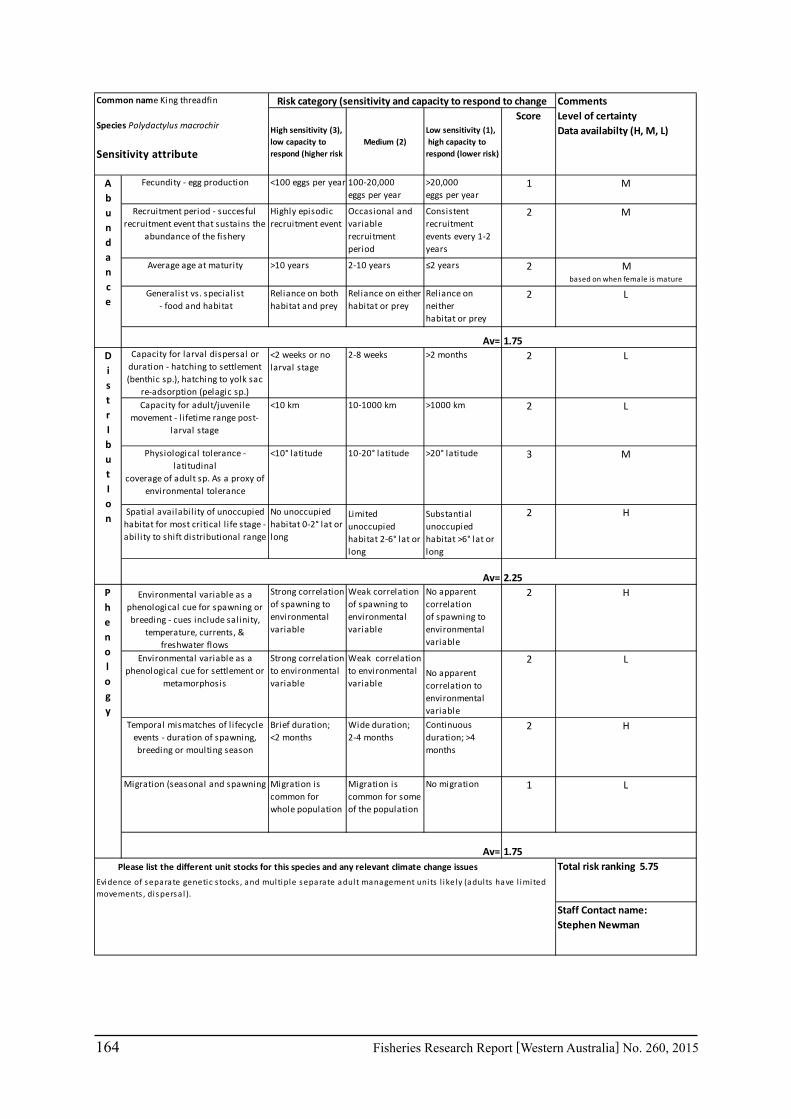
164 Fisheries Research Report [Western Australia] No. 260, 2015
<100 eggs per year 100-20,000eggs per year
>20,000eggs per year
1 M
Highly episodicrecruitment event
Occasional and variable recruitment period
Consistentrecruitment events every 1-2 years
2 M
>10 years 2-10 years ≤2 years 2 Mbased on when female is mature
Reliance on bothhabitat and prey
Reliance on eitherhabitat or prey
Reliance on neitherhabitat or prey
2 L
<2 weeks or nolarval stage
2-8 weeks >2 months 2 L
<10 km 10-1000 km >1000 km 2 L
<10° latitude 10-20° latitude >20° latitude 3 M
No unoccupiedhabitat 0-2° lat or long
Limited unoccupiedhabitat 2-6° lat or long
Substantial unoccupiedhabitat >6° lat or long
2 H
Strong correlationof spawning to environmental variable
Weak correlationof spawning to environmental variable
No apparent correlationof spawning to environmental variable
2 H
Strong correlation to environmental variable
Weak correlation to environmental variable
No apparent correlation to environmental variable
2 L
Brief duration;<2 months
Wide duration;2-4 months
Continuousduration; >4 months
2 H
Migration is common for whole population
Migration is common for some of the population
No migration 1 L
Common name King threadfin
Species Polydactylus macrochir
Sensitivity attribute
Risk category (sensitivity and capacity to respond to change CommentsLevel of certaintyData availabilty (H, M, L)High sensitivity (3),
low capacity to respond (higher risk
Medium (2)Low sensitivity (1), high capacity to respond (lower risk)
Score
Phenology
Environmental variable as aphenological cue for spawning or breeding - cues include salinity,
temperature, currents, & freshwater flows
Environmental variable as a phenological cue for settlement or
metamorphosis
Temporal mismatches of l ifecycleevents - duration of spawning, breeding or moulting season
Migration (seasonal and spawning
Av= 1.75Please list the different unit stocks for this species and any relevant climate change issues Total risk ranking 5.75
Evidence of separate genetic s tocks , and multiple separate adult management uni ts l ikely (adults have l imited movements , dispersa l ).
Abundance
Fecundity - egg production
Recruitment period - succesfulrecruitment event that sustains the
abundance of the fishery
Average age at maturity
Generalist vs. specialist - food and habitat
Av= 1.75DistrIbutIon
Capacity for larval dispersal orduration - hatching to settlement (benthic sp.), hatching to yolk sac
re-adsorption (pelagic sp.)Capacity for adult/juvenile
movement - l ifetime range post-larval stage
Physiological tolerance - latitudinal
coverage of adult sp. As a proxy of environmental tolerance
Spatial availabil ity of unoccupiedhabitat for most critical l ife stage - abil ity to shift distributional range
Av= 2.25
Staff Contact name:Stephen Newman
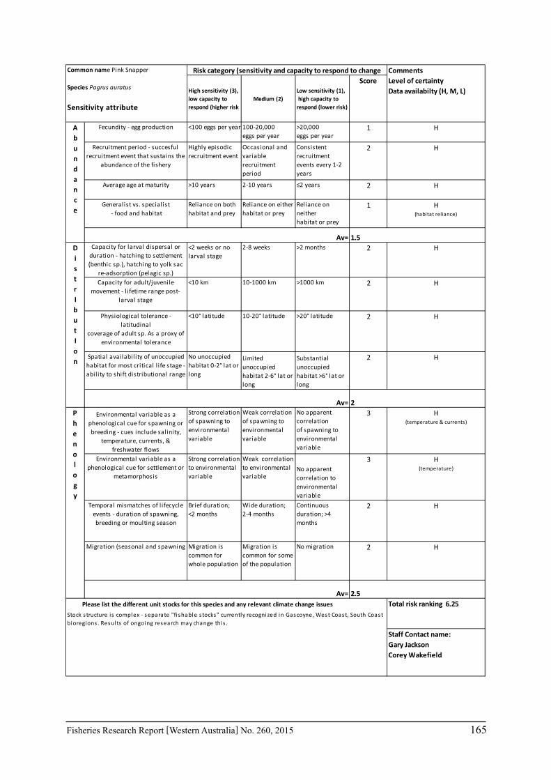
Fisheries Research Report [Western Australia] No. 260, 2015 165
<100 eggs per year 100-20,000eggs per year
>20,000eggs per year
1 H
Highly episodicrecruitment event
Occasional and variable recruitment period
Consistentrecruitment events every 1-2 years
2 H
>10 years 2-10 years ≤2 years 2 H
Reliance on bothhabitat and prey
Reliance on eitherhabitat or prey
Reliance on neitherhabitat or prey
1 H(habitat reliance)
<2 weeks or nolarval stage
2-8 weeks >2 months 2 H
<10 km 10-1000 km >1000 km 2 H
<10° latitude 10-20° latitude >20° latitude 2 H
No unoccupiedhabitat 0-2° lat or long
Limited unoccupiedhabitat 2-6° lat or long
Substantial unoccupiedhabitat >6° lat or long
2 H
Strong correlationof spawning to environmental variable
Weak correlationof spawning to environmental variable
No apparent correlationof spawning to environmental variable
3 H(temperature & currents)
Strong correlation to environmental variable
Weak correlation to environmental variable
No apparent correlation to environmental variable
3 H(temperature)
Brief duration;<2 months
Wide duration;2-4 months
Continuousduration; >4 months
2 H
Migration is common for whole population
Migration is common for some of the population
No migration 2 H
Abundance
Fecundity - egg production
Recruitment period - succesfulrecruitment event that sustains the
abundance of the fishery
Average age at maturity
Generalist vs. specialist - food and habitat
Av= 1.5DistrIbutIon
Capacity for larval dispersal orduration - hatching to settlement (benthic sp.), hatching to yolk sac
re-adsorption (pelagic sp.)Capacity for adult/juvenile
movement - l ifetime range post-larval stage
Physiological tolerance - latitudinal
coverage of adult sp. As a proxy of environmental tolerance
Spatial availabil ity of unoccupiedhabitat for most critical l ife stage - abil ity to shift distributional range
Av= 2
Common name Pink Snapper
Species Pagrus auratus
Sensitivity attribute
Risk category (sensitivity and capacity to respond to change CommentsLevel of certaintyData availabilty (H, M, L)High sensitivity (3),
low capacity to respond (higher risk
Medium (2)Low sensitivity (1), high capacity to respond (lower risk)
Score
Staff Contact name:Gary JacksonCorey Wakefield
Phenology
Environmental variable as aphenological cue for spawning or breeding - cues include salinity,
temperature, currents, & freshwater flows
Environmental variable as a phenological cue for settlement or
metamorphosis
Temporal mismatches of l ifecycleevents - duration of spawning, breeding or moulting season
Migration (seasonal and spawning
Av= 2.5Please list the different unit stocks for this species and any relevant climate change issues Total risk ranking 6.25
Stock s tructure i s complex - separate "fi shable s tocks" currently recognized in Gascoyne, West Coast, South Coast bioregions . Resul ts of ongoing research may change this .
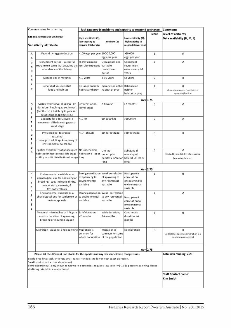
166 Fisheries Research Report [Western Australia] No. 260, 2015
<100 eggs per year 100-20,000eggs per year
>20,000eggs per year
1 M
Highly episodicrecruitment event
Occasional and variable recruitment period
Consistentrecruitment events every 1-2 years
2 M
>10 years 2-10 years ≤2 years 2 H
Reliance on bothhabitat and prey
Reliance on eitherhabitat or prey
Reliance on neitherhabitat or prey
2 Hdependency on very restricted
spawning habitat
<2 weeks or nolarval stage
2-8 weeks >2 months 3 M
<10 km 10-1000 km >1000 km 2 M
<10° latitude 10-20° latitude >20° latitude 3 H
No unoccupiedhabitat 0-2° lat or long
Limited unoccupiedhabitat 2-6° lat or long
Substantial unoccupiedhabitat >6° lat or long
3 Mlimited by availability of estuaries
(spawning habitat)
Strong correlationof spawning to environmental variable
Weak correlationof spawning to environmental variable
No apparent correlationof spawning to environmental variable
3 H
Strong correlation to environmental variable
Weak correlation to environmental variable
No apparent correlation to environmental variable
2 M
Brief duration;<2 months
Wide duration;2-4 months
Continuousduration; >4 months
3 H
Migration is common for whole population
Migration is common for some of the population
No migration 3 HUndertakes spawning migration (an
anadromous species)
Common name Perth herring
Species Nematalosa vlaminghi
Sensitivity attribute
Risk category (sensitivity and capacity to respond to change CommentsLevel of certaintyData availabilty (H, M, L)High sensitivity (3),
low capacity to respond (higher risk
Medium (2)Low sensitivity (1), high capacity to respond (lower risk)
Score
Phenology
Environmental variable as aphenological cue for spawning or breeding - cues include salinity,
temperature, currents, & freshwater flows
Environmental variable as a phenological cue for settlement or
metamorphosis
Temporal mismatches of l ifecycleevents - duration of spawning, breeding or moulting season
Migration (seasonal and spawning
Av= 2.75Please list the different unit stocks for this species and any relevant climate change issues Total risk ranking 7.25
Single breeding s tock, with very smal l range = endemic to lower west coast bioregion.Smal l s tock s i ze (i .e. low abundance).Semi-anadromous; only known to spawn in 3 estuaries , requires low sa l ini ty (~10-15 ppt) for spawning. Hence decl ining ra infa l l i s a major threat.
Abundance
Fecundity - egg production
Recruitment period - succesfulrecruitment event that sustains the
abundance of the fishery
Average age at maturity
Generalist vs. specialist - food and habitat
Av= 1.75DistrIbutIon
Capacity for larval dispersal orduration - hatching to settlement (benthic sp.), hatching to yolk sac
re-adsorption (pelagic sp.)Capacity for adult/juvenile
movement - l ifetime range post-larval stage
Physiological tolerance - latitudinal
coverage of adult sp. As a proxy of environmental tolerance
Spatial availabil ity of unoccupiedhabitat for most critical l ife stage - abil ity to shift distributional range
Av= 2.75
Staff Contact name:Kim Smith

Fisheries Research Report [Western Australia] No. 260, 2015 167
<100 eggs per year 100-20,000eggs per year
>20,000eggs per year
1 H
Highly episodicrecruitment event
Occasional and variable recruitment period
Consistentrecruitment events every 1-2 years
1 H
>10 years 2-10 years ≤2 years 1 H
Reliance on bothhabitat and prey
Reliance on eitherhabitat or prey
Reliance on neitherhabitat or prey
1 M
<2 weeks or nolarval stage
2-8 weeks >2 months 2 H
<10 km 10-1000 km >1000 km 2 M
<10° latitude 10-20° latitude >20° latitude 3 H
No unoccupiedhabitat 0-2° lat or long
Limited unoccupiedhabitat 2-6° lat or long
Substantial unoccupiedhabitat >6° lat or long
2 M
Strong correlationof spawning to environmental variable
Weak correlationof spawning to environmental variable
No apparent correlationof spawning to environmental variable
3 H
Strong correlation to environmental variable
Weak correlation to environmental variable
No apparent correlation to environmental variable
2 H
Brief duration;<2 months
Wide duration;2-4 months
Continuousduration; >4 months
2 H
Migration is common for whole population
Migration is common for some of the population
No migration 2 H
Abundance
Fecundity - egg production
Recruitment period - succesfulrecruitment event that sustains the
abundance of the fishery
Average age at maturity
Generalist vs. specialist - food and habitat
Av= 1DistrIbutIon
Capacity for larval dispersal orduration - hatching to settlement (benthic sp.), hatching to yolk sac
re-adsorption (pelagic sp.)Capacity for adult/juvenile
movement - l ifetime range post-larval stage
Physiological tolerance - latitudinal
coverage of adult sp. As a proxy of environmental tolerance
Spatial availabil ity of unoccupiedhabitat for most critical l ife stage - abil ity to shift distributional range
Av= 2.25
Common name Pilchard
Species Sardinops sagax
Sensitivity attribute
Risk category (sensitivity and capacity to respond to change CommentsLevel of certaintyData availabilty (H, M, L)High sensitivity (3),
low capacity to respond (higher risk
Medium (2)Low sensitivity (1), high capacity to respond (lower risk)
Score
Staff Contact name:Brett MolonyPaul Lewis
Phenology
Environmental variable as aphenological cue for spawning or breeding - cues include salinity,
temperature, currents, & freshwater flows
Environmental variable as a phenological cue for settlement or
metamorphosis
Temporal mismatches of l ifecycleevents - duration of spawning, breeding or moulting season
Migration (seasonal and spawning
Av= 2.25Please list the different unit stocks for this species and any relevant climate change issues Total risk ranking 5.5

168 Fisheries Research Report [Western Australia] No. 260, 2015
<100 eggs per year 100-20,000eggs per year
>20,000eggs per year
1 M
Highly episodicrecruitment event
Occasional and variable recruitment period
Consistentrecruitment events every 1-2 years
2 M
>10 years 2-10 years ≤2 years 2 H
Reliance on bothhabitat and prey
Reliance on eitherhabitat or prey
Reliance on neitherhabitat or prey
1 M
<2 weeks or nolarval stage
2-8 weeks >2 months 2 L
<10 km 10-1000 km >1000 km 2 L
<10° latitude 10-20° latitude >20° latitude 2 M
No unoccupiedhabitat 0-2° lat or long
Limited unoccupiedhabitat 2-6° lat or long
Substantial unoccupiedhabitat >6° lat or long
2 H
Strong correlationof spawning to environmental variable
Weak correlationof spawning to environmental variable
No apparent correlationof spawning to environmental variable
2 H
Strong correlation to environmental variable
Weak correlation to environmental variable
No apparent correlation to environmental variable
2 L
Brief duration;<2 months
Wide duration;2-4 months
Continuousduration; >4 months
2 H
Migration is common for whole population
Migration is common for some of the population
No migration 1 M
Common name Red emperor
Species Lutjanus sebae
Sensitivity attribute
Risk category (sensitivity and capacity to respond to change CommentsLevel of certaintyData availabilty (H, M, L)High sensitivity (3),
low capacity to respond (higher risk
Medium (2)Low sensitivity (1), high capacity to respond (lower risk)
Score
Phenology
Environmental variable as aphenological cue for spawning or breeding - cues include salinity,
temperature, currents, & freshwater flows
Environmental variable as a phenological cue for settlement or
metamorphosis
Temporal mismatches of l ifecycleevents - duration of spawning, breeding or moulting season
Migration (seasonal and spawning
Av= 1.75Please list the different unit stocks for this species and any relevant climate change issues Total risk ranking 5.25
One genetic s tock with multiple separate adult management uni ts (adults have l imited movements ).
Abundance
Fecundity - egg production
Recruitment period - succesfulrecruitment event that sustains the
abundance of the fishery
Average age at maturity
Generalist vs. specialist - food and habitat
Av= 1.5DistrIbutIon
Capacity for larval dispersal orduration - hatching to settlement (benthic sp.), hatching to yolk sac
re-adsorption (pelagic sp.)Capacity for adult/juvenile
movement - l ifetime range post-larval stage
Physiological tolerance - latitudinal
coverage of adult sp. As a proxy of environmental tolerance
Spatial availabil ity of unoccupiedhabitat for most critical l ife stage - abil ity to shift distributional range
Av= 2
Staff Contact name:Stephen Newman

Fisheries Research Report [Western Australia] No. 260, 2015 169
<100 eggs per year 100-20,000eggs per year
>20,000eggs per year
1 H
Highly episodicrecruitment event
Occasional and variable recruitment period
Consistentrecruitment events every 1-2 years
2 M
>10 years 2-10 years ≤2 years 1 H
Reliance on bothhabitat and prey
Reliance on eitherhabitat or prey
Reliance on neitherhabitat or prey
2 M
<2 weeks or nolarval stage
2-8 weeks >2 months 2 H
<10 km 10-1000 km >1000 km 2 H
<10° latitude 10-20° latitude >20° latitude 2 H
No unoccupiedhabitat 0-2° lat or long
Limited unoccupiedhabitat 2-6° lat or long
Substantial unoccupiedhabitat >6° lat or long
1 H(limited juvenile habitats)
Strong correlationof spawning to environmental variable
Weak correlationof spawning to environmental variable
No apparent correlationof spawning to environmental variable
2 L
Strong correlation to environmental variable
Weak correlation to environmental variable
No apparent correlation to environmental variable
2 L
Brief duration;<2 months
Wide duration;2-4 months
Continuousduration; >4 months
2 H
Migration is common for whole population
Migration is common for some of the population
No migration 2 M
Abundance
Fecundity - egg production
Recruitment period - succesfulrecruitment event that sustains the
abundance of the fishery
Average age at maturity
Generalist vs. specialist - food and habitat
Av= 1.5DistrIbutIon
Capacity for larval dispersal orduration - hatching to settlement (benthic sp.), hatching to yolk sac
re-adsorption (pelagic sp.)Capacity for adult/juvenile
movement - l ifetime range post-larval stage
Physiological tolerance - latitudinal
coverage of adult sp. As a proxy of environmental tolerance
Spatial availabil ity of unoccupiedhabitat for most critical l ife stage - abil ity to shift distributional range
Av= 1.75
Common name Spanish Mackerel
Species Scomberomorous commerson
Sensitivity attribute
Risk category (sensitivity and capacity to respond to change CommentsLevel of certaintyData availabilty (H, M, L)High sensitivity (3),
low capacity to respond (higher risk
Medium (2)Low sensitivity (1), high capacity to respond (lower risk)
Score
Staff Contact name:Stephen Newman
Phenology
Environmental variable as aphenological cue for spawning or breeding - cues include salinity,
temperature, currents, & freshwater flows
Environmental variable as a phenological cue for settlement or
metamorphosis
Temporal mismatches of l ifecycleevents - duration of spawning, breeding or moulting season
Migration (seasonal and spawning
Av= 2Please list the different unit stocks for this species and any relevant climate change issues Total risk ranking 5.25
Single breeding population in WA.

170 Fisheries Research Report [Western Australia] No. 260, 2015
<100 eggs per year 100-20,000eggs per year
>20,000eggs per year
1 M
Highly episodicrecruitment event
Occasional and variable recruitment period
Consistentrecruitment events every 1-2 years
2 M
>10 years 2-10 years ≤2 years 2 H
Reliance on bothhabitat and prey
Reliance on eitherhabitat or prey
Reliance on neitherhabitat or prey
2 M
<2 weeks or nolarval stage
2-8 weeks >2 months 2 L
<10 km 10-1000 km >1000 km 2 L
<10° latitude 10-20° latitude >20° latitude 2 M
No unoccupiedhabitat 0-2° lat or long
Limited unoccupiedhabitat 2-6° lat or long
Substantial unoccupiedhabitat >6° lat or long
2 H(limited juvenile habitats)
Strong correlationof spawning to environmental variable
Weak correlationof spawning to environmental variable
No apparent correlationof spawning to environmental variable
2 H
Strong correlation to environmental variable
Weak correlation to environmental variable
No apparent correlation to environmental variable
2 L
Brief duration;<2 months
Wide duration;2-4 months
Continuousduration; >4 months
2 H
Migration is common for whole population
Migration is common for some of the population
No migration 2 M
Common name Spangled emperor
Species Lethrinus nebulosus
Sensitivity attribute
Risk category (sensitivity and capacity to respond to change CommentsLevel of certaintyData availabilty (H, M, L)High sensitivity (3),
low capacity to respond (higher risk
Medium (2)Low sensitivity (1), high capacity to respond (lower risk)
Score
Phenology
Environmental variable as aphenological cue for spawning or breeding - cues include salinity,
temperature, currents, & freshwater flows
Environmental variable as a phenological cue for settlement or
metamorphosis
Temporal mismatches of l ifecycleevents - duration of spawning, breeding or moulting season
Migration (seasonal and spawning
Av= 2Please list the different unit stocks for this species and any relevant climate change issues Total risk ranking 5.75
One genetic s tock with extens ive gene flow, multiple separate adult management uni ts (adults have l imited movements , dispersa l ).
Abundance
Fecundity - egg production
Recruitment period - succesfulrecruitment event that sustains the
abundance of the fishery
Average age at maturity
Generalist vs. specialist - food and habitat
Av= 1.75DistrIbutIon
Capacity for larval dispersal orduration - hatching to settlement (benthic sp.), hatching to yolk sac
re-adsorption (pelagic sp.)Capacity for adult/juvenile
movement - l ifetime range post-larval stage
Physiological tolerance - latitudinal
coverage of adult sp. As a proxy of environmental tolerance
Spatial availabil ity of unoccupiedhabitat for most critical l ife stage - abil ity to shift distributional range
Av= 2
Staff Contact name:Stephen NewmanRoss Marriott
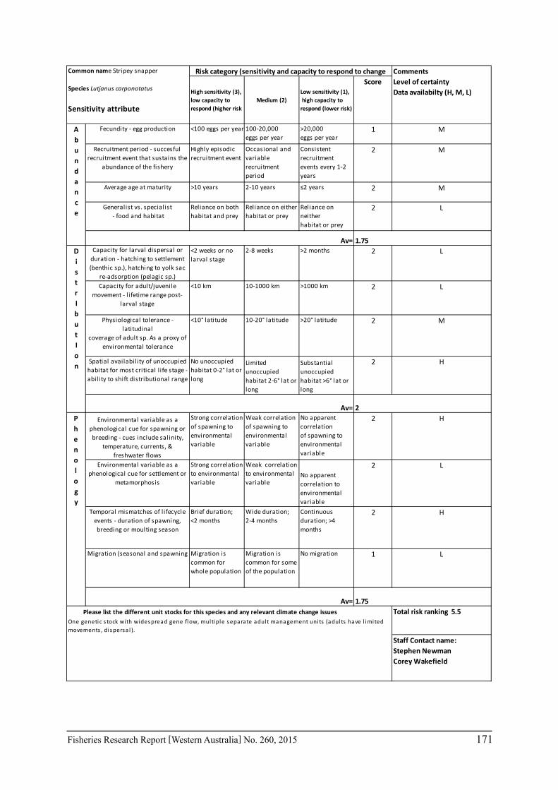
Fisheries Research Report [Western Australia] No. 260, 2015 171
<100 eggs per year 100-20,000eggs per year
>20,000eggs per year
1 M
Highly episodicrecruitment event
Occasional and variable recruitment period
Consistentrecruitment events every 1-2 years
2 M
>10 years 2-10 years ≤2 years 2 M
Reliance on bothhabitat and prey
Reliance on eitherhabitat or prey
Reliance on neitherhabitat or prey
2 L
<2 weeks or nolarval stage
2-8 weeks >2 months 2 L
<10 km 10-1000 km >1000 km 2 L
<10° latitude 10-20° latitude >20° latitude 2 M
No unoccupiedhabitat 0-2° lat or long
Limited unoccupiedhabitat 2-6° lat or long
Substantial unoccupiedhabitat >6° lat or long
2 H
Strong correlationof spawning to environmental variable
Weak correlationof spawning to environmental variable
No apparent correlationof spawning to environmental variable
2 H
Strong correlation to environmental variable
Weak correlation to environmental variable
No apparent correlation to environmental variable
2 L
Brief duration;<2 months
Wide duration;2-4 months
Continuousduration; >4 months
2 H
Migration is common for whole population
Migration is common for some of the population
No migration 1 L
Abundance
Fecundity - egg production
Recruitment period - succesfulrecruitment event that sustains the
abundance of the fishery
Average age at maturity
Generalist vs. specialist - food and habitat
Av= 1.75DistrIbutIon
Capacity for larval dispersal orduration - hatching to settlement (benthic sp.), hatching to yolk sac
re-adsorption (pelagic sp.)Capacity for adult/juvenile
movement - l ifetime range post-larval stage
Physiological tolerance - latitudinal
coverage of adult sp. As a proxy of environmental tolerance
Spatial availabil ity of unoccupiedhabitat for most critical l ife stage - abil ity to shift distributional range
Av= 2
Common name Stripey snapper
Species Lutjanus carponotatus
Sensitivity attribute
Risk category (sensitivity and capacity to respond to change CommentsLevel of certaintyData availabilty (H, M, L)High sensitivity (3),
low capacity to respond (higher risk
Medium (2)Low sensitivity (1), high capacity to respond (lower risk)
Score
Staff Contact name:Stephen NewmanCorey Wakefield
Phenology
Environmental variable as aphenological cue for spawning or breeding - cues include salinity,
temperature, currents, & freshwater flows
Environmental variable as a phenological cue for settlement or
metamorphosis
Temporal mismatches of l ifecycleevents - duration of spawning, breeding or moulting season
Migration (seasonal and spawning
Av= 1.75Please list the different unit stocks for this species and any relevant climate change issues Total risk ranking 5.5
One genetic s tock with widespread gene flow, multiple separate adult management uni ts (adults have l imited movements , dispersa l ).
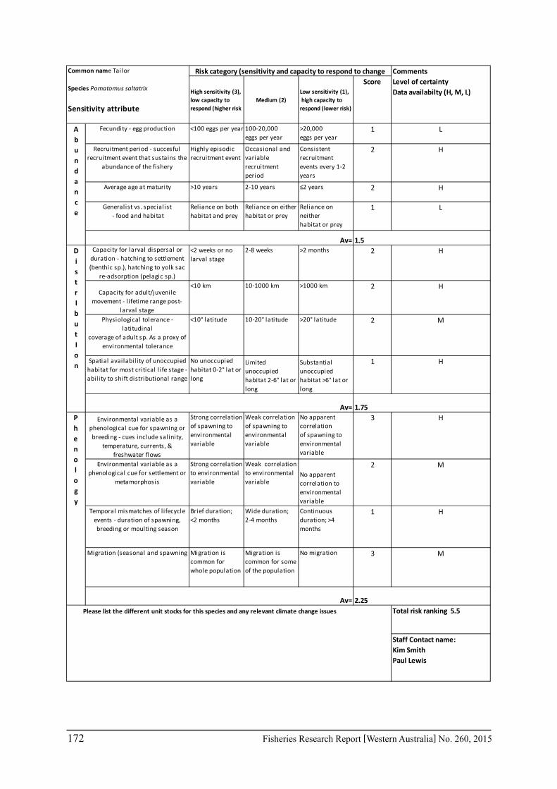
172 Fisheries Research Report [Western Australia] No. 260, 2015
<100 eggs per year 100-20,000eggs per year
>20,000eggs per year
1 L
Highly episodicrecruitment event
Occasional and variable recruitment period
Consistentrecruitment events every 1-2 years
2 H
>10 years 2-10 years ≤2 years 2 H
Reliance on bothhabitat and prey
Reliance on eitherhabitat or prey
Reliance on neitherhabitat or prey
1 L
<2 weeks or nolarval stage
2-8 weeks >2 months 2 H
<10 km 10-1000 km >1000 km 2 H
<10° latitude 10-20° latitude >20° latitude 2 M
No unoccupiedhabitat 0-2° lat or long
Limited unoccupiedhabitat 2-6° lat or long
Substantial unoccupiedhabitat >6° lat or long
1 H
Strong correlationof spawning to environmental variable
Weak correlationof spawning to environmental variable
No apparent correlationof spawning to environmental variable
3 H
Strong correlation to environmental variable
Weak correlation to environmental variable
No apparent correlation to environmental variable
2 M
Brief duration;<2 months
Wide duration;2-4 months
Continuousduration; >4 months
1 H
Migration is common for whole population
Migration is common for some of the population
No migration 3 M
Common name Tailor
Species Pomatomus saltatrix
Sensitivity attribute
Risk category (sensitivity and capacity to respond to change CommentsLevel of certaintyData availabilty (H, M, L)High sensitivity (3),
low capacity to respond (higher risk
Medium (2)Low sensitivity (1), high capacity to respond (lower risk)
Score
Phenology
Environmental variable as aphenological cue for spawning or breeding - cues include salinity,
temperature, currents, & freshwater flows
Environmental variable as a phenological cue for settlement or
metamorphosis
Temporal mismatches of l ifecycleevents - duration of spawning, breeding or moulting season
Migration (seasonal and spawning
Av= 2.25Please list the different unit stocks for this species and any relevant climate change issues Total risk ranking 5.5
Abundance
Fecundity - egg production
Recruitment period - succesfulrecruitment event that sustains the
abundance of the fishery
Average age at maturity
Generalist vs. specialist - food and habitat
Av= 1.5DistrIbutIon
Capacity for larval dispersal orduration - hatching to settlement (benthic sp.), hatching to yolk sac
re-adsorption (pelagic sp.)
Capacity for adult/juvenilemovement - l ifetime range post-
larval stagePhysiological tolerance -
latitudinalcoverage of adult sp. As a proxy of
environmental tolerance
Spatial availabil ity of unoccupiedhabitat for most critical l ife stage - abil ity to shift distributional range
Av= 1.75
Staff Contact name:Kim SmithPaul Lewis

Fisheries Research Report [Western Australia] No. 260, 2015 173
<100 eggs per year 100-20,000eggs per year
>20,000eggs per year
3 H
Highly episodicrecruitment event
Occasional and variable recruitment period
Consistentrecruitment events every 1-2 years
1 L
>10 years 2-10 years ≤2 years 3 H
Reliance on bothhabitat and prey
Reliance on eitherhabitat or prey
Reliance on neitherhabitat or prey
1 H
<2 weeks or nolarval stage
2-8 weeks >2 months 3 H
<10 km 10-1000 km >1000 km 1 M
<10° latitude 10-20° latitude >20° latitude 2 H
No unoccupiedhabitat 0-2° lat or long
Limited unoccupiedhabitat 2-6° lat or long
Substantial unoccupiedhabitat >6° lat or long
1 M
Strong correlationof spawning to environmental variable
Weak correlationof spawning to environmental variable
No apparent correlationof spawning to environmental variable
2 L
Strong correlation to environmental variable
Weak correlation to environmental variable
No apparent correlation to environmental variable
2 L
Brief duration;<2 months
Wide duration;2-4 months
Continuousduration; >4 months
2 H
Migration is common for whole population
Migration is common for some of the population
No migration 3 M
Abundance
Fecundity - egg production
Recruitment period - succesfulrecruitment event that sustains the
abundance of the fishery
Average age at maturity
Generalist vs. specialist - food and habitat
Av= 2DistrIbutIon
Capacity for larval dispersal orduration - hatching to settlement (benthic sp.), hatching to yolk sac
re-adsorption (pelagic sp.)
Capacity for adult/juvenilemovement - l ifetime range post-
larval stagePhysiological tolerance -
latitudinalcoverage of adult sp. As a proxy of
environmental tolerance
Spatial availabil ity of unoccupiedhabitat for most critical l ife stage - abil ity to shift distributional range
Av= 1.5
Common name Thickskin
Species Carcharhinus plumbeus
Sensitivity attribute
Risk category (sensitivity and capacity to respond to change CommentsLevel of certaintyData availabilty (H, M, L)High sensitivity (3),
low capacity to respond (higher risk
Medium (2)Low sensitivity (1), high capacity to respond (lower risk)
Score
Staff Contact name:Rory McAuleyMatias Braccini
Phenology
Environmental variable as aphenological cue for spawning or breeding - cues include salinity,
temperature, currents, & freshwater flows
Environmental variable as a phenological cue for settlement or
metamorphosis
Temporal mismatches of l ifecycleevents - duration of spawning, breeding or moulting season
Migration (seasonal and spawning
Av= 2.25Please list the different unit stocks for this species and any relevant climate change issues Total risk ranking 5.75

174 Fisheries Research Report [Western Australia] No. 260, 2015
<100 eggs per year 100-20,000eggs per year
>20,000eggs per year
1 H
Highly episodicrecruitment event
Occasional and variable recruitment period
Consistentrecruitment events every 1-2 years
2 H
>10 years 2-10 years ≤2 years 2 H
Reliance on bothhabitat and prey
Reliance on eitherhabitat or prey
Reliance on neitherhabitat or prey
2 H
<2 weeks or nolarval stage
2-8 weeks >2 months 2 M
<10 km 10-1000 km >1000 km 2 H
<10° latitude 10-20° latitude >20° latitude 3 H
No unoccupiedhabitat 0-2° lat or long
Limited unoccupiedhabitat 2-6° lat or long
Substantial unoccupiedhabitat >6° lat or long
2 H
Strong correlationof spawning to environmental variable
Weak correlationof spawning to environmental variable
No apparent correlationof spawning to environmental variable
3 H
Strong correlation to environmental variable
Weak correlation to environmental variable
No apparent correlation to environmental variable
3 L
Brief duration;<2 months
Wide duration;2-4 months
Continuousduration; >4 months
2 H
Migration is common for whole population
Migration is common for some of the population
No migration 1 H
Common name WA Dhufish
Species Glaucosoma hebraicum
Sensitivity attribute
Risk category (sensitivity and capacity to respond to change CommentsLevel of certaintyData availabilty (H, M, L)High sensitivity (3),
low capacity to respond (higher risk
Medium (2)Low sensitivity (1), high capacity to respond (lower risk)
Score
Phenology
Environmental variable as aphenological cue for spawning or breeding - cues include salinity,
temperature, currents, & freshwater flows
Environmental variable as a phenological cue for settlement or
metamorphosis
Temporal mismatches of l ifecycleevents - duration of spawning, breeding or moulting season
Migration (seasonal and spawning
Av= 1.75Please list the different unit stocks for this species and any relevant climate change issues Total risk ranking 5.75
Abundance
Fecundity - egg production
Recruitment period - succesfulrecruitment event that sustains the
abundance of the fishery
Average age at maturity
Generalist vs. specialist - food and habitat
Av= 1.75DistrIbutIon
Capacity for larval dispersal orduration - hatching to settlement (benthic sp.), hatching to yolk sac
re-adsorption (pelagic sp.)
Capacity for adult/juvenilemovement - l ifetime range post-
larval stagePhysiological tolerance -
latitudinalcoverage of adult sp. As a proxy of
environmental tolerance
Spatial availabil ity of unoccupiedhabitat for most critical l ife stage - abil ity to shift distributional range
Av= 2.25
Staff Contact name:David Fairclough

Fisheries Research Report [Western Australia] No. 260, 2015 175
<100 eggs per year 100-20,000eggs per year
>20,000eggs per year
1 L
Highly episodicrecruitment event
Occasional and variable recruitment period
Consistentrecruitment events every 1-2 years
2 H
>10 years 2-10 years ≤2 years 3 Hprotogynous hermaphrodite
Reliance on bothhabitat and prey
Reliance on eitherhabitat or prey
Reliance on neitherhabitat or prey
1 HForager with ontogenetic diet change
<2 weeks or nolarval stage
2-8 weeks >2 months 2 L
<10 km 10-1000 km >1000 km 3 HSmall home range with high site fidelity
<10° latitude 10-20° latitude >20° latitude 3 HRestricted to south of Abrolhos Islands
No unoccupiedhabitat 0-2° lat or long
Limited unoccupiedhabitat 2-6° lat or long
Substantial unoccupiedhabitat >6° lat or long
1 L
Strong correlationof spawning to environmental variable
Weak correlationof spawning to environmental variable
No apparent correlationof spawning to environmental variable
3 HStrongest recruitment in years of weak
Leeuwin Current
Strong correlation to environmental variable
Weak correlation to environmental variable
No apparent correlation to environmental variable
1 L
Brief duration;<2 months
Wide duration;2-4 months
Continuousduration; >4 months
1 HSpawning June to October
Migration is common for whole population
Migration is common for some of the population
No migration 1 HOntogentic movement inshore-offshore
Abundance
Fecundity - egg production
Recruitment period - succesfulrecruitment event that sustains the
abundance of the fishery
Average age at maturity
Generalist vs. specialist - food and habitat
Av= 1.75DistrIbutIon
Capacity for larval dispersal orduration - hatching to settlement (benthic sp.), hatching to yolk sac
re-adsorption (pelagic sp.)
Capacity for adult/juvenilemovement - l ifetime range post-
larval stagePhysiological tolerance -
latitudinalcoverage of adult sp. As a proxy of
environmental tolerance
Spatial availabil ity of unoccupiedhabitat for most critical l ife stage - abil ity to shift distributional range
Av= 2.25
Common name Western blue groper
Species Achoerodus gouldii
Sensitivity attribute
Risk category (sensitivity and capacity to respond to change CommentsLevel of certaintyData availabilty (H, M, L)High sensitivity (3),
low capacity to respond (higher risk
Medium (2)Low sensitivity (1), high capacity to respond (lower risk)
Score
Very long l ived (max age 70 years )Staff Contact name:Jeffrey NorrissPeter Coulson
Phenology
Environmental variable as aphenological cue for spawning or breeding - cues include salinity,
temperature, currents, & freshwater flows
Environmental variable as a phenological cue for settlement or
metamorphosis
Temporal mismatches of l ifecycleevents - duration of spawning, breeding or moulting season
Migration (seasonal and spawning
Av= 1.75Please list the different unit stocks for this species and any relevant climate change issues Total risk ranking 5.75
Poor recrui tment in years of s trong Leeuwin Current.
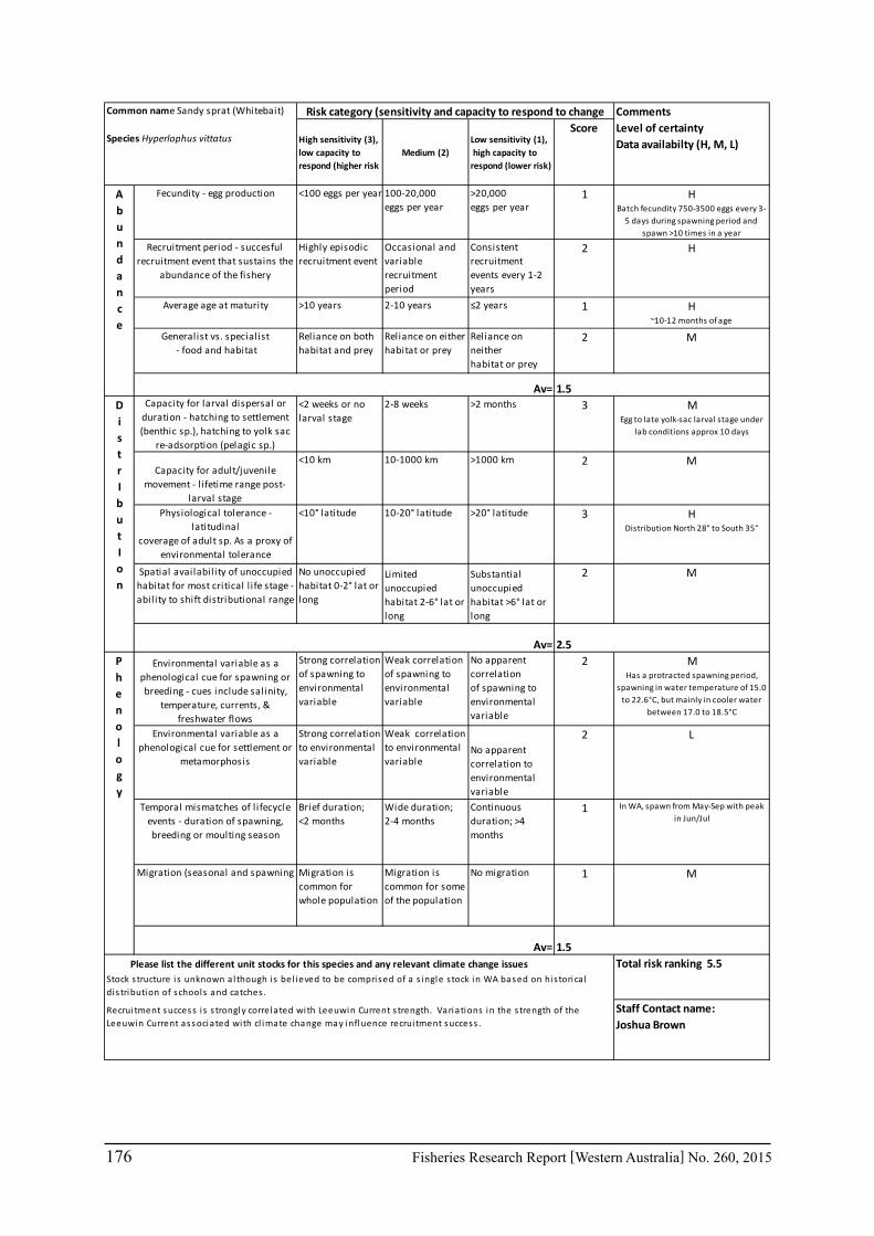
176 Fisheries Research Report [Western Australia] No. 260, 2015
<100 eggs per year 100-20,000eggs per year
>20,000eggs per year
1 HBatch fecundity 750-3500 eggs every 3-
5 days during spawning period and spawn >10 times in a year
Highly episodicrecruitment event
Occasional and variable recruitment period
Consistentrecruitment events every 1-2 years
2 H
>10 years 2-10 years ≤2 years 1 H~10-12 months of age
Reliance on bothhabitat and prey
Reliance on eitherhabitat or prey
Reliance on neitherhabitat or prey
2 M
<2 weeks or nolarval stage
2-8 weeks >2 months 3 MEgg to late yolk-sac larval stage under
lab conditions approx 10 days
<10 km 10-1000 km >1000 km 2 M
<10° latitude 10-20° latitude >20° latitude 3 HDistribution North 28° to South 35°
No unoccupiedhabitat 0-2° lat or long
Limited unoccupiedhabitat 2-6° lat or long
Substantial unoccupiedhabitat >6° lat or long
2 M
Strong correlationof spawning to environmental variable
Weak correlationof spawning to environmental variable
No apparent correlationof spawning to environmental variable
2 MHas a protracted spawning period,
spawning in water temperature of 15.0 to 22.6°C, but mainly in cooler water
between 17.0 to 18.5°C
Strong correlation to environmental variable
Weak correlation to environmental variable
No apparent correlation to environmental variable
2 L
Brief duration;<2 months
Wide duration;2-4 months
Continuousduration; >4 months
1 In WA, spawn from May-Sep with peak in Jun/Jul
Migration is common for whole population
Migration is common for some of the population
No migration 1 M
Common name Sandy sprat (Whitebait)
Species Hyperlophus vittatus
Risk category (sensitivity and capacity to respond to change CommentsLevel of certaintyData availabilty (H, M, L)High sensitivity (3),
low capacity to respond (higher risk
Medium (2)Low sensitivity (1), high capacity to respond (lower risk)
Score
Recrui tment success i s s trongly correlated with Leeuwin Current s trength. Variations in the s trength of the Leeuwin Current associated with cl imate change may influence recrui tment success .
Staff Contact name:Joshua Brown
Phenology
Environmental variable as aphenological cue for spawning or breeding - cues include salinity,
temperature, currents, & freshwater flows
Environmental variable as a phenological cue for settlement or
metamorphosis
Temporal mismatches of l ifecycleevents - duration of spawning, breeding or moulting season
Migration (seasonal and spawning
Av= 1.5Please list the different unit stocks for this species and any relevant climate change issues Total risk ranking 5.5
Stock s tructure i s unknown a l though i s bel ieved to be comprised of a s ingle s tock in WA based on his torica l dis tribution of schools and catches .
Abundance
Fecundity - egg production
Recruitment period - succesfulrecruitment event that sustains the
abundance of the fishery
Average age at maturity
Generalist vs. specialist - food and habitat
Av= 1.5DistrIbutIon
Capacity for larval dispersal orduration - hatching to settlement (benthic sp.), hatching to yolk sac
re-adsorption (pelagic sp.)
Capacity for adult/juvenilemovement - l ifetime range post-
larval stagePhysiological tolerance -
latitudinalcoverage of adult sp. As a proxy of
environmental tolerance
Spatial availabil ity of unoccupiedhabitat for most critical l ife stage - abil ity to shift distributional range
Av= 2.5