Lidar inversion with variable backscatter/extinction ratios

James D. Klett

The conventional approach to solving the single-scattering lidar equation makes use of the assumption ofa power law relation between backscatter and extinction with a fixed exponent and constant of proportional-ity. An alternative formulation is given herein which assumes the proportionality factor in the power lawrelationship is itself a function of range or extinction. The resulting lidar equation is solvable as before, andexamples are given to show how even an approximate description of deviations from the power law form canyield an improved inversion solution for the extinction. A further generalization is given which includes theeffects of a background of Rayleigh scatterers.

1. Introduction

The volume extinction [(k)] and backscatter [(k)]coefficients at wave number k due to particulate scat-tering and absorption are given by integrals over the sizedistribution n(r) of (assumed spherical) particles ofradius r:

v(k) = 7r fr2Q(rh,kr)n(r)dr,

f,(k) = 7r fr2Q,r(ml,kr)n(r)dr,

(1)

(2)

where Q and Q, are, respectively, the extinction andbackscatter efficiencies, as determined by the Mietheory of scattering; both are functions of the complexindex of refraction mh and size parameter kr. (Gaseousabsorption contributions to are not included in thispaper.) It is clear from their definition as weightedintegrals over the size distribution that the ratio ofbackscatter to extinction will be, for a given wavelengthand complex index, only a function of the shape of thedistribution. (Shape here simply refers to the sizedistribution known to within an arbitrary scale factor.)Therefore, if the spectral shape and composition of thescattering aerosol are spatially invariant, so too will bethe proportionality between and . On the otherhand, if the aerosol spectral form or composition doesvary with location, and cr can be regarded as havinga proportionality which is range dependent.

The author is with PAR Associates, 1077 La Quinta, Las Cruces,New Mexico 88005.

Received 10 September 1984.0003-6935/85/111638-06$02.00/0.© 1985 Optical Society of America.

The traditional way to account for any dependencebetween :3 and o- is to assume a power law relationshipof the form

= Boak, (3)

where Bo and k are constants, but k is no longer unity.Then the single-backscattering lidar equation may, withthe use of Eq. (3), be reduced to the form

dS 1 d_ = -- -2cdr dr

k dua= -- - 2a,a dr

(4)

(5)

with S(r) = ln[r2P(r)], and where P(r) is the power re-ceived from range r. The stable solution to Eq. (5) is

v(r) =exp[(S - Sm)/k]

la + eprm [(S -Sm)k]dr'l(6)

where Sm = S(rm), e m =-(rm), and r < rm.1 In addi-tion to requiring the validity of Eq. (3) and the absenceof multiple scattering, Eq. (6) also assumes that gaseousabsorption effects are negligible.

From the discussion preceding Eq. (3) it is clear thatit would be more realistic to regard and ai as linearlyrelated but with a proportionality which is itself afunction of range or extinction. An approximate andsimple way of formulating the inversion problem in thisfashion is given in this paper. Any available informa-tion concerning deviations from a strict linear rela-tionship can be easily incorporated into the solutionimplementation. An example of the backscatter/ex-tinction variation for water clouds is given, and it isshown how even a very approximate description of thisvariation can yield an improved inversion solution forthe extinction. Finally, a further generalization iscarried out which includes the effects of a backgroundof Rayleigh scatterers.

1638 APPLIED OPTICS / Vol. 24, No. 11 / 1 June 1985

II. Modified Inversion Solution for Variable B 10

Suppose now that 3 and a are related according to 9

Bak (7)where B is a function of r, and k is a constant. (Fromthe discussion above one would generally set k = 1, but 6

it is retained here as a fixed parameter primarily tofacilitate direct comparison below between new and old 4

expressions.) Then on substitution of this expression 3

into Eq. (4) one finds 2

dS ldB+kd-2a, (8) ldr B dr a dr

ord(S-lnB) kdr-= --- 2. (9)

dr or dr

But this is the same as Eq. (5) except that S is now re-placed by S - nB. Hence one can write down the so-lution immediately in the form of Eq. (6):

a(r) =exp(S - Sm - nB + lnBm)/k]

I + .fr exp[(S-Sm-lnB + lnBm)Ikldr'1(10)

or

a(r) =(Bm/B)l/k exp[(S - Sm)/k_

I (11)

Ilo-; + 2 S (Bm/B)l/k exp[(S - Sm)Ik]dr'I

where Bm = B (rm).An apparent difficulty with Eq. (11) is that in general

we cannot expect to know B (r) precisely until we alsoknow v(r); i.e., it is really part of the solution. However,an approximate solution to Eq. (11), still more accuratethan the default version with Bm/B = 1 [i.e., Eq. (6)],can be obtained if there is available at least some in-formation on the dependence of B on either r or a-.Suppose, for example, that for the aerosol in questionthere has been established an approximate empiricalcorrelation of the form B = f(a). Then an approximatesolution can be obtained by a two (or more if needed)-stage iteration: First, letBm/B = 1 and solve Eq. (11)or (6) to obtain the first-order solution ul. Second,solve Eq. (11) for the second-order solution U2, wherenow we use

B(r) = f[a, ( r). (12)

We shall now turn to an example of this approach andcompare the outcome with the familiar method basedon Eqs. (3) and (6).

Ill. Inversion Examples for Conditions of Fog andLow Clouds

An example of the variability of B with range forconditions of fog and low clouds is shown in Fig. 1. Thedata displayed (supplied by E. Measures, AtmosphericSciences Laboratory, White Sands Missile Range, N.M.88002, personal communication) derives from in situmeasurements made by balloon-borne particle countersin Meppen, Germany, in the fall of 1980.23 Mie theorywas applied at a wavelength of 1.06 Am to obtain profileswith height of /3 and cr under the assumption that the

MEPPEN I

NORMRLIZED BRCKSCRTTER/EXTINCTION

100 200 300 400HEIGHT (meters)

500

Fig. 1. Dependence on range of backscatter-to-extinction ratio forlow stratus cloud in Meppen, Germany, 1980. Ratio normalized byvalue at near range point Zo. Data based on in situ measurementsof drop size distributions. Light wavelength = 1.06 m (adaptedfrom calculations of E. Measures, ASL/WSMR; personal

communication).

1 00 .

100

10

L

E0

LU

E

MEU

*0

z

.1

. 01

.001

1 10 100RRDIUS (micrometers)

Fig. 2. Drop size distributions from in-cloud measurements inMeppen, Germany, 1980. The eight distributions shown are averagesfor the following labeled ranges of extinction (km): 1, (0.1,0.6); 2,(0.6,1.5); 3, (1.5,3); 4, (3,15); 5, (15,40); 6, (40,65); 7, (65,100); 8,

(100,200) (from Ref. 3).

particles were spherical drops of pure water. A set ofcharacteristic aerosol spectra obtained by these mea-surements for various extinction intervals is shown inFig. 2.3

It is evident in Fig. 2 that the data may be somewhatincomplete, as the distributions are truncated at smallsizes where the particle concentrations are still high.This spectral truncation is due to limited instrumentalresolution. In addition, one should perhaps take intoaccount the variation of mh with size; for example, thepresence of soot particles in the smaller droplets maysignificantly affect their optical properties.4 5 But inspite of these limitations, the data shown serve well toindicate the kind of behavior that is expected to occurtypically. The trends shown in Fig. 2 are, for example,quite consistent with what one expects for water clouds,

1 June 1985 / Vol. 24, No. 11 / APPLIED OPTICS 1639

, . .

, I I I I I

MEPPEN I B vs In SIGMR (Ga

n N - 61 -

I I | In SIGMR

Fig. 3. Log-Gaussian fit [Eq. (13)] of backscatter to extinction ratiovs extinction for Meppen data.

MEPPEN I DRTR

1 .00

0.00

-1.00

-2.00 +

4 -3.00M

-4.00

-5. +

-6.00 v

-7.00 +

X) a) X) X C) X 6) ID 61

C., N - 61 - N In C t)I 7

In SIGMR

Fig. 4. Dependence of backscatter-to-extinction ratio on extinctionfor Meppen data.

16

14

E 1 2

Lf 10 8

4

2

100 200 300 400 500HEIGHT (meters)

Fig. 5. Simulated relative range-corrected logarithmic signal, S -Sm [Eq. (14)], for Meppen data.

ussian it) namely, that the drop spectrum will evolve toward abimodal shape and a larger average drop size with in-creasing liquid water content.6 The continuing flow ofwater mass up the size spectrum to larger drops is alsoexpected to be positively correlated with increasingextinction, especially if condensation continues to re-plenish the spectrum at small drop sizes. Such con-tinued production of small drops by condensation anddiffusional growth is to be expected for actively growingclouds with an evolving bimodal drop distribution aslong as an upward flux of moist air continues.

From the profiles of and a described above one canalso obtain an empirical correlation between B and a.

X9 0 s This is shown in Fig. 3, where a lognormal curve hasNU (T1 t been fitted to a total of nine data pairs; the equation of

the curve is

f(u) = 0.0074 + 0.055 expl-[(lna - 4)/3.1]21. (13)

One may alternatively use linear regression applied toa plot of:3 and al to find values for Bo and k in the powerlaw expression of Eq. (3). The best fit line is shown inFig. 4 and has the parameters Bo = 0.017 and k = 1.34.The basis for the departure from k = 1 can be discernedby comparing Figs. 2 and 4. The plotted data in thelatter figure tend to trace out a slightly undulatingcurve, the ends of which have a smaller slope (k nearunity) than the middle section. This correspondsqualitatively to the similar unimodal shapes of spectra1-3 and the similar bimodal shapes of spectra 6-8 in Fig.2. Such behavior is consistent with the expectation thatk = 1 over any interval where the spectral shape is in-variant, as discussed above. In general, it is thechanging proportionality between /3 and with chang-ing spectral composition or shape that causes anyoverall power law description of /(o-) to produce k #1.

By integration of Eq. (4) the relative signal, S - Sm,appearing in the inversion solution may be obtained asa function of :3 and a:

S-Sm=ln - +2 Jr. cdr',(3m

(14)

where Om = /(rm). Then by substituting the calculatedprofiles of :3(r) and a(r) for the Meppen data, a simu-lation of the relative signal is available (Fig. 5) fromwhich one may in turn use Eq. (6) or (11) to attempt toretrieve v(r) for various choices of k or B. For thepurpose of this paper the correct value for em will beassumed as a given quantity. (The sometimes formi-dable but separate problem of estimating elm lies outsidethe scope ofAhis paper.)

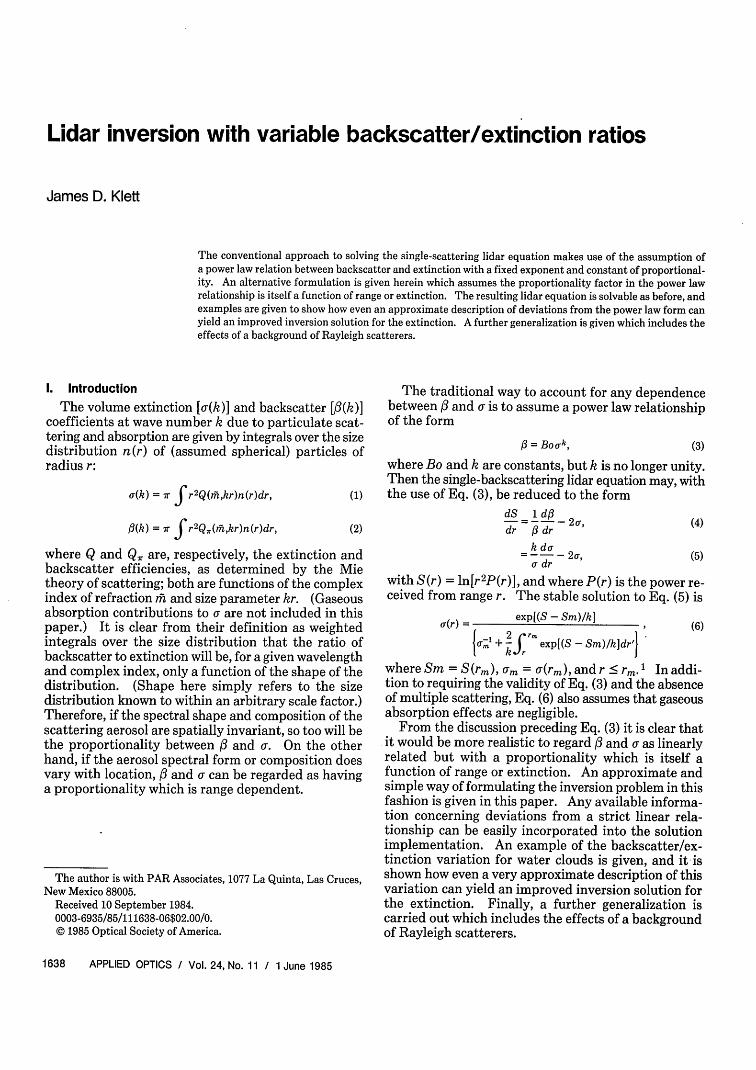
Let us firstconsider use of Eq. (6) with k = 1 or 1.3.The inversion results shown in Figs. 6 and 7 demon-strate that the better choice is k = 1.3, as expected fromthe previous fit of the data to the power law form.(Results like those shown in Figs. 6 and 7 have beenobtained previously and independently from theMeppen data by E. Measures, ASL/WSMR; privatecommunication.) The solution for k = 1 is seen tooverestimate the extinction by nearly an order of mag-nitude in the first 250 m, where the visibility is high.

1640 APPLIED OPTICS / Vol. 24, No. 11 / 1 June 1985

.10

.09

.0B

.07

.06

m .05

.04

.03

.02

.01

0.00

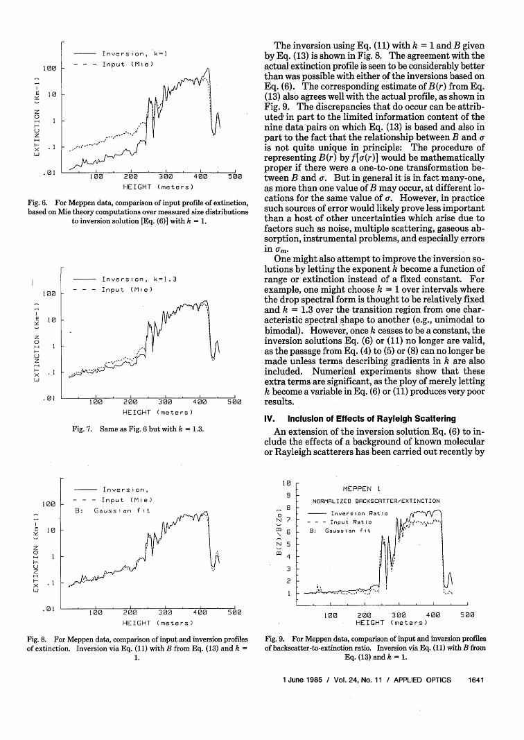
The inversion using Eq. (11) with k = 1 and B givenInversion, k=1 by Eq. (13) is shown in Fig. 8. The agreement with the

100 - - - Input (Mie) actual extinction profile is seen to be considerably betterthan was possible with either of the inversions based on

E n < 1 Eq. (6). The corresponding estimate of B (r) from Eq.x 1 0 _ i, ̂ jU 1 (13) also agrees well with the actual profile, as shown in

Fig. 9. The discrepancies that do occur can be attrib-1 uted in part to the limited information content of the

U ., 1 l U nine data pairs on which Eq. (13) is based and also inZ -- part to the fact that the relationship between B and

.1 is not quite unique in principle: The procedure ofrepresenting B(r) by f [(r)] would be mathematically

.01 0 2 0 0 , proper if there were a one-to-one transformation be-100 200 300 400 500 tween B and a. But in general it is in fact many-one,

HEIGHT (meters) as more than one value of B may occur, at different lo-

Fig. 6. For Meppen data, comparison of input profile of extinction, cations for the same value of a. However, in practicebased on Mie theory computations over measured size distributions such sources of error would likely prove less important

to inversion solution [Eq. (6)] with k = 1. than a host of other uncertainties which arise due tofactors such as noise, multiple scattering, gaseous ab-sorption, instrumental problems, and especially errorsin am.

One might also attempt to improve the inversion so-lutions by letting the exponent k become a function of

Inversion, k=1.3 range or extinction instead of a fixed constant. For

100 - - - Input (Mie) example, one might choose k = 1 over intervals whereg00 \the drop spectral form is thought to be relatively fixed

and k = 1.3 over the transition region from one char-E 10 acteristic spectral shape to another (e.g., unimodal to

1 1719t i bimodal). However, once k ceases to be a constant, the0 l / l q inversion solutions Eq. (6) or (11) no longer are valid,

as the passage from Eq. (4) to (5) or (8) can no longer bez <; HI made unless terms describing gradients in k are alsox * l -included. Numerical experiments show that these

extra terms are significant, as the ploy of merely letting.01 , 0 k become a variable in Eq. (6) or (11) produces very poor

100 200 300 400 500 results.HEIGHT (meters)

IV. Inclusion of Effects of Rayleigh ScatteringFig. 7. Same as Fig. 6 but with k = 1.3. An extension of the inversion solution Eq. (6) to in-

clude the effects of a background of known molecularor Rayleigh scatterers has been carried out recently by

10Inversion, MEPPEN 1

9

100 - - - Input (Mie) I NORMRLIZED BCKSCRTTER/EXTINCTION_.B: Gaussian fit LO 8InesoRail

.0 10 200 Gausia fit0 00 20 30 0 0Fig. 8. or Meppn datacomparisn of inut andInversion Rrfls Fg .Fr e ndtcmaionfiptadivrinpoie

0

.'~~~~~~.1 1q 1 )a dk= 1

Z 3

X

.01 ~100 200 300 400 500 100 200 300 400 500

HEIGHT (meters) HEIGHT (meters)

Fig. 8. For Meppen data, comparison of input and inversion profiles Fig. 9. For Meppen data, comparison of input and inversion profilesof extinction. Inversion via Eq. (11) with Bfrom Eq. (13) and k= of backscatter-to-extinction ratio. nversion via Eq. (11) with Bfromn

1. Eq. (13) and k = 1.

1 June 1985 / Vol. 24, No. 11 / APPLIED OPTICS 1641

Fernald.7 In this section a similar extermodified inversion solution Eq. (11) wiloped.

Let the total backscatter coefficient bas

(r) = Bp(r)ap(r) + BRCR(Z),with

BR 3/(87r),

Bp(r) f[ap(r)].

Subscripts P and R refer to the aerosol Rayleigh contributions, respectively. Thdescribes the fixed backscatter-to-extinctRayleigh scatterers, while Eq. (17) descritfor the particles according to formulation ofthe function f(up) being the empirical cortween Bp and up. Also the Rayleigh extincient uR(Z) is assumed to be a known functiz.

On substituting Eq. (15) into the basicential equation, Eq. (4), and noting also tlUp + UR, we obtain

dS 1 d: - 2(BPlflp + BR1(3R),dr 3#dr

= 1 d3 2B_'( + 2(B- 1- B)flR.

(3dr B R

Therefore, if one defines a new signal vari,

S'-Sm' = S-Sm + 2 fr- (3Rdr' -2 frBR

Eq. (19) can be rearranged to read as follo

dS' 1 d 2(3

dr ( dr Bp

But this has the same form as Eq. (5), expresence of the function Bp(r). The solutiocan, therefore, be constructed in the same fa(6) to obtain

/3(r =exp(S' - Sm')

[-31 + 2 r. exp(S'- Sm')dr'

Eqs. (20) and (22) comprise the solution to stated at the beginning of the section. No- 0, Eq. (11) is recovered (with k = 1). Sinis a constant, Eq. (22) becomes equivalenttion obtained by Fernald.7

Implementation of Eqs. (20) and (22) wethe procedures already described. Exan,application of this model will be presentechere the goal has been merely to present f(particular generalization to show how a kground level of scattering could be includemulation of Sec. II.

V. Discussion

A new theoretical framework has been pdealing with the problem of variations i:scatter-to-extinction ratio that occur becai

ision of the tions in aerosol particle composition or spectral shape.I be devel- It has been shown that if this ratio can be empirically

correlated with extinction magnitude, this informatione expressed can then be incorporated into a modified stable inver-

sion solution to improve the accuracy of retrieved ex-tinction profiles. With this physically direct and simpleapproach the backscatter/extinction ratio becomes amodulating factor in an otherwise linear relationship

(16) between backscatter and extinction.(17) The familiar alternative approach, whereby infor-

mation on backscatter and extinction is cast in the form)article and of an empirical power law relationship, has a less directius Eqti f physical justification but nevertheless also has practicalt ratio r value with respect to the accuracy of retrieved profiless the ratith of extinction so long as the exponent is a constant rep-

Sec. i, wt resentative of all the empirical data. However, at-inection be- tempts to refine the inversion solutions by letting thection coeffi- exponent become a variable parameter are ill-advised,on of height as the available solution forms no longer apply, andlidar differ- serious errors may result.ila nowfe- a An example has been given of an aerosol for which thehat now Uf = backscatter/extinction ratio could be described ap-

proximately as a function of extinction [Eq. (13) andl18) Fig. 3]. This was provided as an illustration of the

(18) technique of incorporating information on departuresfrom a linear relationship between and a to invoke the

(19) new inversion solution. The functional forrp of the,ble S as particular example chosen was, of course, not intended

ible 5' as to be viewed as a universally applicable relationship.(3rdr' (20) Nevertheless, some of its shape characteristics were

BP ' found to be qualitatively as expected, and similar rea-ws: soning based on such factors as meteorological condi-

tions, or the source and age of the aerosol, might simi-(21) larly provide some insight into the approximate devia-

tions from a linear relationship between and incept for the various real applications.n to Eq. (21) It should also be noted that great precision in theshion as Eq. functional description for /l is not required to obtain

useful results. As many numerical simulations haveshown, even if nothing is known about the aerosol, the

(22) standard default assumption that and U are propor-tional may be used to obtain extinction profiles thatoften reflect surprisingly well the qualitative and

the problem quantitative trends of the actual distributions. Thiste that if /3R is fundamentally a consequence of the stability of thelilarly, if Bp solution form given by Eq. (6). (The contrary assertionto the solu- that :/3 must be very accurately known to get any

useful information on el is still made occasionally, butiuld parallel this is an erroneous notion that first came about fromiples of the studies based on the unstable form of the lidar inversion1 elsewhere; solution. The hazards of that approach in general and)rmally this in the context of the relationship between backscatternown back- and extinction have been discussed elsewhere.1 )d in the for- Mathematically speaking, the present formulation

relaxes the previous requirement that any account,theoretical or experimental, of the relationship betweenbackscatter and extinction must be cast into an ap-proximate power law form to make use of the standard

resented for inversion solution. With Eq. (11) any functional form,a the back- / = f'(u) can be used to obtain quickly an approximateise of varia- solution for U by substituting B = f'(l)/l in Eq. (11) and

1642 APPLIED OPTICS / Vol. 24, No. 11 / 1 June 1985

iterating a few times as described in Sec. II. As asimple example, the usual solution based on the powerlaw form of Eq. (3) may be recovered by substituting B= Bok-l into Eq. (11) and iterating.

Finally, the numerical examples given in this papersuggest that for the same amount of aerosol scatteringinformation, the modulated backscatter/extinction ratioapproach gives better results than the power law for-mulation. Further study of the new modified inversionsolution will of course be required to assess more fullyits practical utility.

This work was performed under contract to the U.S.Army Atmospheric Sciences Laboratory, White SandsMissile Range, N.M. 88002.

References1. J. D. Klett, "Stable Analytical Inversion Solution for Processing

Lidar Returns," Appl. Opt. 20, 211 (1981).2. J. D. Lindberg, Ed., "Early Wintertime European Fog and Haze:

Report on Project Meppen 80," ASL-TR-0108, U.S. Army Atmo-spheric Sciences Laboratory, White Sands Missile Range, N.M.88002 (1982).

3. J. D. Lindberg, R. B. Loveland, L. D. Duncan, M. B. Richardson,and J. Esparza, "Vertical Profiles of Extinction and Particle SizeDistribution Measurements Made in European Wintertime Fogand Haze," ASL-TR-0151, U.S. Army Atmospheric SciencesLaboratory, White Sands Missile Range, N.M. 88002 (1984).

4. J. W. Fitzgerald, "Effect of Relative Humidity on the AerosolBackscattering Coefficient at 0.694- and 10.6-m Wavelengths,"Appl. Opt. 23, 411 (1984).

5. C. F. Bohren, and D. R. Huffman, Absorption and Scattering ofLight by Small Particles (Wiley, New York, 1983), 530 pp.

6. H. R. Pruppacher and J. D. Klett, Microphysics of Clouds andPrecipitation (Reidel, Dordrecht, Holland, 1978), 714 pp.

7. F. G. Fernald, "Analysis of Atmospheric Lidar Observations:Some Comments," Appl. Opt. 23, 652 (1984).

Meetings Calendar continued from page 1584

1985June

24-28 Optical Signal Processing course, Troy Off. of Con-tinuing Studies, Rensselaer Polytechnic Inst., Troy,N.Y. 12180

24-29 Fourier & Computerized Infrared Spectroscopy Int.Conf., Ottawa Natl. Res. Council of Canada, L.Baignee, Conf. Services Off., Ottawa, Ontario, CanadaKIA OR6

24-5 July Applied Optics Summer course, London J. Dainty,Optics Sec., Blackett Lab., Imperial Coll., LondonSW7 2BZ, England

24-5 July Applied Materials Technology: Materials Processing forProcess-Sensitive Manufacturing course, EdinburghOff. of Summer Session, Rm. E19-356, MIT, Cam-bridge, Mass. 02139

25-27 11th Int. Symp. on Machine Processing of RemotelySensed Data, West Lafayette D. Morrison, PurdueU./LARS, 1291 Cumberland Ave., West Lafayette,Ind. 47906

26-28 Int. Congr. on Lasers in Medicine & Surgery, BolognaMedicina Viva, Viale dei Mille, 140, 43100 Parma,Italy

26-28 Local Area Networks course, Wash., D.C. Data-TechInst., Lakeview Plaza, P.O. Box 2429, Clifton, N.J.07015

8-10 Flow Visualization Techniques: Principles & Applica-tions course, Ann Arbor Eng. Summer Confs., 200Chrysler Ctr., N. Campus, U. of Mich., Ann Arbor,Mich. 48109

8-11 3rd Conf. on Coherent Laser Radar: Technology & Ap-plications, Malvern J. Vaughan, Royal Signals &Radar Establishment, Ministry of Defense, St. An-drews Rd., PD316, Great Malvern, Worcestershire,WR14 3PS, U.K.

8-12 17th Int. Conf. on Phenomena in Ionized Glasses, Buda-pest I. Abonyi Roland Eotvos Physical Soc., P.O. Box240, 1368 Budapest, Hungary

8-12 Synthetic Aperture Radar Technology & Applicationscourse, Ann Arbor Eng. Summer Confs., 200 ChryslerCtr., N. Campus, U. of Mich., Ann Arbor, Mich.48109

8-12 Laser Fundamentals & Systems course, Wash., D.C.Eng. Tech., Inc., P.O. Box 8859, Waco, Tex. 76714

8-12 Infrared Spectroscopy: Interpretation of Spectra course,Brunswick D. Mayo, Chem. Dept., Bowdoin Coll.,Brunswick, Me. 04011

8-12 Quality Control for Photographic Processing course,Rochester J. Compton, RIT, P.O. Box 9887, Roches-ter,N.Y. 14623

8-12 Laser Fundamentals & Systems course, Dallas Eng.Tech., Inc., P.O. Box 8859, Waco, Tex. 76714

July

1-4 Int. Conf. on Dynamical Processes in Excited States ofSolids, Villeurbanne W. Yen, U. of Wisconsin,Physics Dept., 1150 University Ave., Madison, Wisc.53706

3-4 Introduction to Military Thermal Imaging course, KentSIRA, Ltd. Conf. Unit, South Hill, Chislehurst, KenBR7 5EH, England

8-19 Lasers & Optics for Applications course, CambridgeMIT, Res. Lab. of Electronics, Cambridge, Mass.02139

9 ISDN Markets course, Arlington Communications &Info. Inst., co Info. Gatekeepers, Inc., 214 HarvardAve., Boston, Mass. 02134

continued on page 1656

1 June 1985 / Vol. 24, No. 11 / APPLIED OPTICS 1643