retrieval of aerosol backscatter and extinction from ... · pdf fileretrieval of aerosol...

Atmos. Meas. Tech., 8, 2909–2926, 2015

www.atmos-meas-tech.net/8/2909/2015/

doi:10.5194/amt-8-2909-2015

© Author(s) 2015. CC Attribution 3.0 License.

Retrieval of aerosol backscatter and extinction from airborne

coherent Doppler wind lidar measurements

F. Chouza1, O. Reitebuch1, S. Groß1, S. Rahm1, V. Freudenthaler2, C. Toledano3, and B. Weinzierl1,2

1Deutsches Zentrum für Luft- und Raumfahrt (DLR), Institut für Physik der Atmosphäre, Oberpfaffenhofen, Germany2Ludwig-Maximilians-Universität München (LMU), Meteorologisches Institut, München, Germany3University of Valladolid, Atmospheric Optics Group, Valladolid, Spain

Correspondence to: F. Chouza ([email protected])

Received: 29 January 2015 – Published in Atmos. Meas. Tech. Discuss.: 18 February 2015

Revised: 9 June 2015 – Accepted: 16 June 2015 – Published: 21 July 2015

Abstract. A novel method for calibration and quantitative

aerosol optical property retrieval from Doppler wind lidars

(DWLs) is presented in this work. Due to the strong wave-

length dependence of the atmospheric molecular backscatter

and the low sensitivity of the coherent DWLs to spectrally

broad signals, calibration methods for aerosol lidars cannot

be applied to coherent DWLs usually operating at wave-

lengths between 1.5 and 2 µm. Instead, concurrent measure-

ments of an airborne DWL at 2 µm and the POLIS ground-

based aerosol lidar at 532 nm are used in this work, in com-

bination with sun photometer measurements, for the calibra-

tion and retrieval of aerosol backscatter and extinction pro-

files at 532 nm.

The proposed method was applied to measurements from

the SALTRACE experiment in June–July 2013, which aimed

at quantifying the aerosol transport and change in aerosol

properties from the Sahara desert to the Caribbean. The re-

trieved backscatter and extinction coefficient profiles from

the airborne DWL are within 20 % of POLIS aerosol lidar

and CALIPSO satellite measurements. Thus the proposed

method extends the capabilities of coherent DWLs to mea-

sure profiles of the horizontal and vertical wind towards

aerosol backscatter and extinction profiles, which is of high

benefit for aerosol transport studies.

1 Introduction

Mineral dust plays a key role in the climate system. About

half of the annually emitted aerosol mass is mineral dust

(e.g., Hinds 1999) which disturbs the radiation budget, acts

as cloud and ice nuclei and is observed to modify the cloud

glaciation process (e.g., Seifert et al., 2010).

The Saharan desert has been identified as the world’s

largest source of mineral dust (e.g., Mahowald et al., 2005).

Saharan dust is regularly transported westwards across the

Atlantic Ocean (e.g., Prospero, 1999), covering huge ar-

eas of the Atlantic Ocean with the dust-containing Saharan

Air Layer (SAL). Despite the progress made during the last

years, many key questions about the transport, deposition

mechanisms and transformation of the Saharan dust remain

unanswered (Ansmann et al., 2011).

To study the aging and modification of Saharan min-

eral dust during long-range transport from the Sahara

across the Atlantic Ocean into the Caribbean and inves-

tigate the impact of aged mineral dust on the radiation

budget and cloud evolution processes, the Saharan Aerosol

Long-range Transport and Aerosol-Cloud-Interaction Exper-

iment (SALTRACE: http://www.pa.op.dlr.de/saltrace) was

performed in June/July 2013. SALTRACE was designed as a

closure experiment combining a set of ground-based lidar, in

situ and sun photometer instruments deployed on Barbados

(main SALTRACE supersite), Cape Verde and Puerto Rico

with airborne aerosol and wind measurements of the DLR

(Deutsches Zentrum für Luft- und Raumfahrt) research air-

craft Falcon, satellite observations and model simulations.

Altogether 31 research flights were conducted between 10

June and 15 July 2013. For the first time, an airborne 2 µm

Doppler wind lidar (DWL) was deployed to study the dust

transport across the Atlantic Ocean. While airborne DWLs

were mainly used in the past for atmospheric dynamical stud-

ies providing the horizontal wind vector and turbulence mea-

Published by Copernicus Publications on behalf of the European Geosciences Union.

http://www.pa.op.dlr.de/saltrace

2910 F. Chouza et al.: Backscatter and extinction retrieval from Doppler wind lidar

surements (Reitebuch, 2012; Weissmann et al., 2005; Sma-

likho, 2003; Reitebuch et al., 2001), they were also used

to obtain qualitative aerosol data (Bou Karam et al., 2008;

Schumann et al., 2011; Weinzierl et al., 2012). Quantita-

tive aerosol optical properties derived from airborne coherent

DWLs, like backscatter and extinction coefficient, are rarely

reported (Menzies and Tratt, 1994).

The calibration of aerosol lidars is usually performed us-

ing the Rayleigh molecular backscatter from the stratosphere

or the high troposphere (Fernald et al., 1984; Klett, 1985;

Böckmann et al., 2004). However, this method is not appli-

cable to a coherent DWL operating at a wavelength of 2 µm.

The main reason for that are the low intensity of the molec-

ular backscatter, caused by the strong dependence of the

Rayleigh backscatter intensity on the lidar operation wave-

length (P ∝ λ−4), and the low sensitivity of the coherent

DWLs to spectrally broad signals (Henderson et al., 2005).

The latter is a consequence of the DWL’s design to match the

spectrally narrow aerosol return signal to increase the signal-

to-noise ratio.

Up to now, different approaches were used to retrieve cal-

ibrated atmospheric parameters from coherent lidars which

are not suitable to be calibrated using molecular background

as a reference. Most of these techniques rely on the use of the

return signals from targets with known optical properties, in-

cluding ground-based hard targets (Menzies and Tratt, 1994),

sea surface (Bufton et al., 1983) and ground return (Cutten et

al., 2002).

The main problems associated with the calibration of a co-

herent DWL at ground using calibrated targets (Menzies and

Tratt, 1994) are the variability in the optical transmission of

the boundary layer, the effect of the turbulence in the het-

erodyning efficiency, the limitations of the calibration range

due to target size restrictions and the necessity of a well-

characterized system heterodyne efficiency. This last prob-

lem is related to practical limitations in the distance at which

the target can be placed. For usual distances (< 1 km) the li-

dar is not operating in far field regime and a correction has

to be applied taking into account the heterodyne efficiency

function. However, the use of different hard targets such as

flame-sprayed aluminium or sandpaper allows the character-

ization of the system depolarization effects and, through the

use of moving targets, of the system response to return signal

frequency shifts.

The use of sea and ground returns for the calibration of

airborne lidars (Bufton et al., 1983; Cutten et al., 2002)

avoids some of the previously described problems at the cost

of losing some of the advantages of ground-based targets.

The refractive turbulence effects are lower because the path-

integrated turbulence is smaller and the heterodyne efficiency

function is not essential for the calibration procedure because

the ground or sea surface is normally in the region of far field

regime. The use of ground return allows also us to perform a

continuous calibration, with the instrument operating in nor-

mal measuring conditions. Nevertheless, the optical proper-

ties of the ground and sea returns have a higher uncertainty

and are highly variable between different locations. In the

case of the sea surface, they are affected by the wind and

the consequent generation of waves and whitecaps (Li et al.,

2010), while in the case of the ground return relatively con-

stant optical properties are limited to specific regions.

A third method, developed to calibrate cloud lidars

(O’Connor et al., 2004), consists in scaling the backscatter

signal to match the derived lidar ratio with the theoretical

lidar ratio corresponding to stratocumulus clouds. This re-

quires the presence of homogeneous and well-characterized

stratocumulus clouds.

The aim of this paper is to provide an alternative cali-

bration method for coherent DWLs. As the combination of

ground-based and airborne lidars is a usual approach for large

field campaigns aiming at the characterization of aerosols

and its transport (Heintzenberg, 2009; Ansmann et al., 2011),

the availability of simultaneous airborne and ground-based

measurements opens the possibility to a new DWL calibra-

tion method. The proposed method relies on the measure-

ment of the same atmospheric volume by two different lidars:

a reference aerosol lidar to which the Klett–Fernald method

can be applied and the coherent DWL to be calibrated. Based

on simultaneous measurements, calibration constants corre-

sponding to different aerosol types are calculated. Those con-

stants can be then applied to retrieve calibrated backscatter

and extinction coefficient profiles from the coherent DWL

measurements during other flight periods. With the proposed

method, not only can information on horizontal and vertical

wind vector and transport of the aerosol layers be derived

from the (airborne) DWL but synchronous aerosol backscat-

ter and extinction coefficients can also be retrieved.

The paper is organized as follows. Section 2 provides

a brief description of the coherent DWL mounted on the

Falcon research aircraft of DLR during SALTRACE and

an outline of the acquired signal processing. Section 3 de-

scribes the instrumental corrections, calibration and retrieval

method. Section 4 gives a description of the measurement

sets used for the calibration and validation of the method.

Section 5 shows the results of the method applied to parts

of the SALTRACE measurement set. Finally, a summary and

relevant conclusions are presented in Sect. 6.

2 Coherent DWL instrument

2.1 Instrument description

The airborne coherent DWL used during SALTRACE is

based on an instrument from CLR Photonics (Henderson et

al., 1993), today Lockheed Martin Coherent Technologies

(LMCT), together with a scanning and acquisition system

developed by DLR (Köpp et al., 2004) which provides air-

borne wind measurement capabilities. The lidar operates at

a wavelength of 2.02254 µm, with a pulse full width at half

Atmos. Meas. Tech., 8, 2909–2926, 2015 www.atmos-meas-tech.net/8/2909/2015/

F. Chouza et al.: Backscatter and extinction retrieval from Doppler wind lidar 2911

maximum of 400 ns, a pulse energy of 1–2 mJ and a repeti-

tion frequency of 500 Hz. The key system specifications are

summarized in Table 1.

The system is composed of three units: first, a transceiver

head holding the diode pumped solid-state Tm:LuAG laser,

the 10.8 cm diameter afocal transceiver telescope, the re-

ceiver optics and detectors and a double wedge scanner; sec-

ond, a rack with the laser power supply and the cooling unit;

third, another rack that contains the data acquisition and con-

trol electronics.

The system is deployed in the DLR Falcon 20 research

aircraft in order to provide horizontal and vertical wind pro-

files as well as backscatter measurements. The transceiver

head is mounted above the aircraft optical window point-

ing downwards to allow the measurement of vertical profiles

(Fig. 1). The aircraft window consists of a 400 mm diameter

and 35 mm thick INFRASIL-302 fused silica window with

an antireflection coating which was optimized for an angle

of incidence of 10◦.

While single wedge scanners are only able to perform con-

ical scans with a fixed off-nadir angle, the double wedge

scanner used in this system (Käsler et al., 2010) allows us to

perform arbitrary scanning patterns. Typically, for airborne

measurements the lidar is operated in two modes: step-stare

scanning and nadir pointing. The step-stare scanning mode

consists of 24 lines of sight (LOS) I in a conical distribution

with an off-nadir angle of 20◦and a staring duration of 1 s per

LOS direction. This configuration allows the measurement

of horizontal wind speeds with a horizontal resolution of ap-

proximately 6 km, depending on aircraft ground speed. How-

ever, when the system is operated in nadir pointing mode, the

system LOS is kept fixed downwards pointing, while the ac-

cumulation period of 1 s remains the same as for the scanning

mode. The nadir pointing mode allows the system to retrieve

vertical wind profiles with a horizontal resolution of 200 m.

In order to minimize the horizontal wind projection over I

when the system is operating in nadir pointing mode, the

transceiver head was mounted with a pitch angle θm of −2◦.

Together with a variable deflection provided by the scanner

θs (which can be set by the operator during flight), the system

can compensate the aircraft pitch angle θp and provide nadir

pointing measurements I = n.

2.2 Coherent lidar signal equation

The following subsection discusses the properties and the

analysis steps applied to the signal measured by the DWL in

order to obtain a magnitude proportional to the atmospheric

backscattered power.

The coherent DWL operation relies on the heterodyning

technique. The frequency of the light scattered in the atmo-

sphere, fs = f0+fD, is affected by the Doppler effect, which

introduces a frequency shift fD to the laser pulse frequency

f0 proportional to the projection of the relative speed vLOS

between the laser source and the backscattering aerosols on

Table 1. Key parameters of the DWL.

Laser Laser type Solid-state Tm:LuAG

Operation wavelength 2.02254 µm

Laser energy 1–2 mJ

Repetition rate 500 Hz

Pulse length

(full width at half maximum) 400 ns

Frequency offset (fIF) 102 MHz

Transceiver Telescope type Off-axis

Telescope diameter 10.8 cm

Focal length Afocal

Beam diameter (1/e2) 8 cm

Transmitted polarization Circular

Detected polarization Co-polarized

Scanner Type Double wedge

Material Fused silica

Aircraft window Material INFRASIL-302

Coating Anti-reflection (10◦)

Diameter/thickness 400/35 mm

Data acquisition Sampling rate 500 MHz

Resolution 8 bits

Mode Single shot acquisition

the laser pulse direction, with fD = 2vLOSf0c−1. A positive

frequency shift fD indicates a positive relative speed vLOS,

which, in turn, indicates that the scattering aerosols are mov-

ing towards the lidar. For the case of an airborne downward

pointing lidar, this sign convention leads to positive rela-

tive speeds for upward winds and negative relative speeds

for downward winds. The atmospheric backscattered frac-

tion of the outgoing pulse is mixed with a frequency shifted

fm = f0+ fIF sample of the same local oscillator (LO) used

for seeding the outgoing pulse. As a result, the mixed sig-

nal contains one spectral component with a frequency equal

to the sum of the atmospheric backscatter frequency and

the shifted LO frequency fs+ fm and another component

with a frequency equal to the difference of both frequen-

cies 1f= fs− fm = fD+ fIF. Due to the limited detector

bandwidth, only the component with frequency 1f can be

detected. Knowing the frequency of the LO and the shift ap-

plied to the LO (fIF), it is possible to calculate the shift on

the backscatter due to the Doppler effect.

Several authors (e.g., Sonnenschein and Horrigan, 1971;

Frehlich and Kavaya, 1991) describe the coherent DWL in

different levels of generality. In this work, we will focus

on the received power for the specific case of a monos-

tatic pulsed coherent lidar. For a detector with uniform re-

sponse, the signal photocurrent generated by the atmospheric

backscatter can be written as (Henderson et al., 2005)

ih (t)= 2ηqe

hf0

√ηLOPLOηh (t)Psd,I (t)cos(2π1f t +1θ (t)), (1)

where ih is the output current from the detector, t the elapsed

time since the laser trigger, ηq the quantum efficiency, e the

electron charge, h the Planck constant, f0 the laser frequency,

ηh the heterodyne efficiency, ηLO the local oscillator trunca-

www.atmos-meas-tech.net/8/2909/2015/ Atmos. Meas. Tech., 8, 2909–2926, 2015


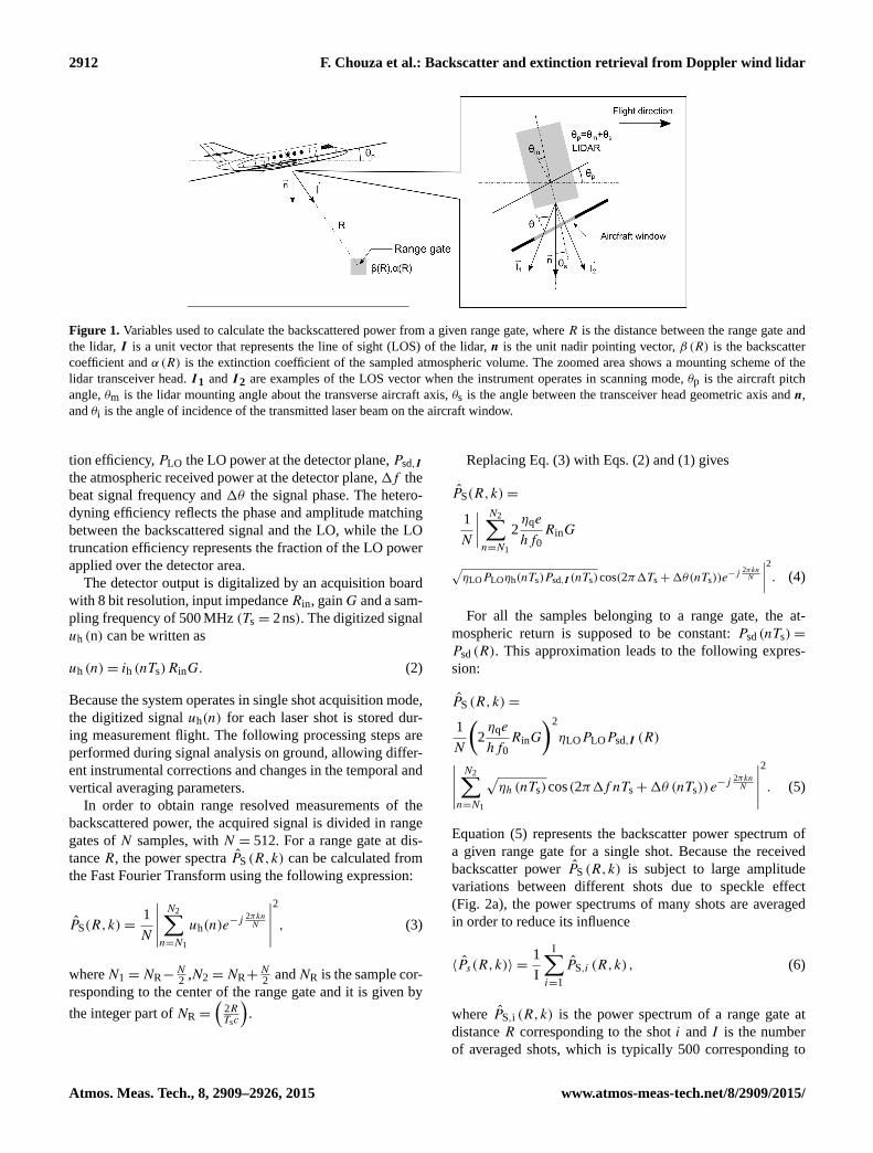
Figure 1. Variables used to calculate the backscattered power from a given range gate, where R is the distance between the range gate and

the lidar, I is a unit vector that represents the line of sight (LOS) of the lidar, n is the unit nadir pointing vector, β (R) is the backscatter

coefficient and α (R) is the extinction coefficient of the sampled atmospheric volume. The zoomed area shows a mounting scheme of the

lidar transceiver head. I1 and I2 are examples of the LOS vector when the instrument operates in scanning mode, θp is the aircraft pitch

angle, θm is the lidar mounting angle about the transverse aircraft axis, θs is the angle between the transceiver head geometric axis and n,

and θi is the angle of incidence of the transmitted laser beam on the aircraft window.

tion efficiency, PLO the LO power at the detector plane, Psd,I

the atmospheric received power at the detector plane,1f the

beat signal frequency and 1θ the signal phase. The hetero-

dyning efficiency reflects the phase and amplitude matching

between the backscattered signal and the LO, while the LO

truncation efficiency represents the fraction of the LO power

applied over the detector area.

The detector output is digitalized by an acquisition board

with 8 bit resolution, input impedanceRin, gainG and a sam-

pling frequency of 500 MHz (Ts = 2ns). The digitized signal

uh (n) can be written as

uh (n)= ih (nTs)RinG. (2)

Because the system operates in single shot acquisition mode,

the digitized signal uh(n) for each laser shot is stored dur-

ing measurement flight. The following processing steps are

performed during signal analysis on ground, allowing differ-

ent instrumental corrections and changes in the temporal and

vertical averaging parameters.

In order to obtain range resolved measurements of the

backscattered power, the acquired signal is divided in range

gates of N samples, with N = 512. For a range gate at dis-

tance R, the power spectra P̂S (R,k) can be calculated from

the Fast Fourier Transform using the following expression:

P̂S(R,k)=1

N

∣∣∣∣∣ N2∑n=N1

uh(n)e−j 2πkn

N

∣∣∣∣∣2

, (3)

whereN1 =NR−N2

,N2 =NR+N2

andNR is the sample cor-

responding to the center of the range gate and it is given by

the integer part of NR =

(2RTsc

).

Replacing Eq. (3) with Eqs. (2) and (1) gives

P̂S(R,k)=

1

N

∣∣∣∣ N2∑n=N1

2ηqe

hf0

RinG

√ηLOPLOηh(nTs)Psd,I (nTs)cos(2π1Ts+1θ(nTs))e

−j 2πknN

∣∣∣∣2. (4)

For all the samples belonging to a range gate, the at-

mospheric return is supposed to be constant: Psd (nTs)=

Psd (R). This approximation leads to the following expres-

sion:

P̂S (R,k)=

1

N

(2ηqe

hf0

RinG

)2

ηLOPLOPsd,I (R)∣∣∣∣∣ N2∑n=N1

√ηh (nTs)cos(2π1fnTs+1θ (nTs))e

−j 2πknN

∣∣∣∣∣2

. (5)

Equation (5) represents the backscatter power spectrum of

a given range gate for a single shot. Because the received

backscatter power P̂S (R,k) is subject to large amplitude

variations between different shots due to speckle effect

(Fig. 2a), the power spectrums of many shots are averaged

in order to reduce its influence

〈P̂s(R,k)〉 =1

I

I∑i=1

P̂S,i (R,k), (6)

where P̂S,i (R,k) is the power spectrum of a range gate at

distance R corresponding to the shot i and I is the number

of averaged shots, which is typically 500 corresponding to



the temporal average over 1 s. Figure 2b illustrates the expo-

nential probability density distribution corresponding to the

received power of a ground return range gate for 500 shots.

Finally, in order to estimate the backscattered power for

the averaged range gates, the summation of the power spec-

tra components around the spectral maximum is performed.

For the sake of simplicity, the noise affecting the system was

omitted from the previous equations. During the processing,

the noise floor is subtracted from the averaged power spectra

before estimating the backscattered power.

The expected value for the backscatter power correspond-

ing to the averaged range gates is calculated through the in-

tegration of the average backscatter power spectrum:

〈P(R)〉 =

K2∑k=K1

〈P̂ (R,k)〉 =

1

N

(2ηqe

hf0

RinG

)2

ηLOPLOηh (R)Psd,I (R), (7)

whereK1 = kmax−K2

,K2 = kmax+K2

, kmax is the index cor-

responding to the maximum of the power spectra and K is

the width of the spectral peak corresponding to the backscat-

tered signal. The optimal value for the integration window

widthK is the one that exactly matches the return pulse spec-

tral width. A shorter integration window will lead to an un-

derestimation of the backscattered power, while a longer in-

tegration window increases the estimation error due to the

integration of measurement noise. Based on these facts, the

integration window width K was set to be 6 (approximately

6 MHz).

Because each power spectra 〈P̂s(R,k)〉 is calculated based

on the average of 500 shots and the received power for a sin-

gle shot follows an exponential probability density function,

the mean received power 〈P(R)〉 can be modeled as a gamma

function. If 500 shots are averaged, the resulting average re-

ceived power relative standard deviation is lower than 5 %.

The received atmospheric power Psd, for a given lidar line

of sight I , can be written as

Psd,I (R)= kin,I (R)ET

AR

R2

c

2β (R)T 2(R), (8)

where kin,I (R) condenses different instrumental constants,

ET is the mean transmitted energy of the averaged laser

pulses, AR is the telescope area, c is the speed of light, β

is the backscatter coefficient and T the atmospheric trans-

mission.

Combining all constants in one constant kd , replacing

Eq. (8) into Eq. (7) and applying a range correction multiply-

ing the backscattered power of each range gate by its squared

distance to the lidar, Eq. (7) can be rewritten as

〈P(R)〉R2= kdETkin,I (R)ηh (R)β (R)T

2(R), (9)

where kd =1N

(2ηqe

hf0RinG

)2

ηLOPLOARc2

.

Figure 2. (a) Power spectra of single shots (dashed) and the aver-

aged spectrum of 500 shots (solid) for the range gate corresponding

to the ground return Rg, an acquisition frequency of 500 MHz and

an Fast Fourier Transform length of 512 samples. (b) Exponential

distribution for the maximum of the power spectra P̂S

(Rg,kmax

)for 500 shots and the range gate Rg.

3 Calibration and retrieval method

3.1 Instrumental corrections

In order to establish the lidar calibration constants (Sect. 3.3),

it is necessary to remove the effect of all the instrumental pa-

rameters that change during the measurement, i.e., the laser

pulse energy ET, the heterodyne efficiency and the instru-

mental constants summarized by kin,I (R).

To remove the dependency of the measured atmospheric

signal power on the fluctuation of the laser energy, the range-

corrected signal is divided by the averaged outgoing laser

pulse energy ET corresponding to all the shots averaged to

calculate the backscattered power. Although the outgoing

pulse energy is not directly measured, a part of each outgo-

ing pulse is mixed with the LO and the resulting beat signal

is stored as frequency reference. The time elapsed between

the laser Q-switch trigger and the amplitude maximum of the

digitized beat signal corresponds to the pulse build-up time.

Based on laboratory measurements (LMCT, personal com-

munication) of the outgoing pulse energy as function of the

Q-Switch build-up time (Fig. 3), it is possible to estimate the

energy ET of the outgoing pulses during the lidar operation.

The laser pulse energy-corrected signal is obtained from

Eq. (9),

〈P(R)〉R2

ET

= kdkin,I (R)ηh (R)β (R)T2(R), (10)

where the instrumental constant kin,I (R) can be expressed as

follows:

kin,I (R)= kGkh (1f )kθ (I )kδ (R), (11)

with kG the acquisition board attenuator, kh (1f ) the system

gain as a function of the backscattered signal frequency 1f ,



Figure 3. Measured and interpolated pulse energy as a function of

the build-up time.

kθ (I ) the change in the received power as a function of the

line of sight angle of incidence on the aircraft window θi

(Fig. 1) and kδ (R) the detector response depending on the

depolarization of the backscattered signal.

The effect of the acquisition board attenuator kG can be

calculated based on the values stored by the acquisition soft-

ware.

To estimate the change in the heterodyne efficiency ηh as a

function of the rangeR, measurements corresponding to a set

of range gates with the same altitude and similar instrumental

constants and atmospheric optical properties were used. The

measurements, performed during flight periods for which the

aircraft was changing its altitude, show the change of the re-

ceived power as a function of the range gate distance R due

to the variation of the heterodyne efficiency in the near field

regime (Fig. 4). Due to sampling of the outgoing laser pulse,

atmospheric range gates at distances lower than 500 m are not

digitized. For this reason, the proposed method is applicable

only if the extinction corresponding to those range gates can

be considered 0 or can be estimated from other sources.

Nonetheless, neglecting the turbulence effects and assum-

ing a monostatic afocal untruncated Gaussian beam lidar, the

heterodyne efficiency change as a function of the rangeR can

be approximated with the following expression (Henderson

et al., 2005):

ηh (R)=

[1+

(πρ2

λR

)2]−1

, (12)

where ρ is the 1/e2 irradiance beam radius and λ the laser

wavelength. Based on the specifications presented in Table 1

and Eq. (12), the expected heterodyne efficiency was calcu-

lated and compared with the measured one (Fig. 4). It can be

seen that the expected heterodyne efficiency is much lower

than the measured one, suggesting that some of the assump-

tions are not applicable for this case. In order to get a practi-

cal correction of the heterodyne efficiency the same function

was fit to the measured backscatter power, leaving πρ2/λ

as optimization parameter. The resulting correction function

Figure 4. Estimated (red, dashed) and derived (red, solid) het-

erodyne efficiency ηh as a function of range R. The normalized

backscatter data points (blue dots) correspond to the averaged

backscatter power corresponding to range gates at altitudes between

4.5 and 5 km for a flight altitude between 5.5 and 8 km during the

flights on 22 June and 11 July.

is (Fig. 4)

ηh (R)=

[1+

(621.5

R

)2]−1

. (13)

The heterodyne efficiency corrected signal can be obtained

from Eqs. (10) and (13):

〈P(R)〉R2

ETηh (R)= kdkin,I (R)β (R)T

2(R). (14)

According to Eq. (13), for range gates corresponding to

ranges R larger than 3500 m, which is the case of the mea-

surements presented in this work (Table 2), the heterodyne

efficiency is almost constant (less than 3 % variation) and the

system can be considered operating in far field regime with a

constant heterodyne efficiency ηh (R)= ηh.

A sample of the received atmospheric backscattered power

after applying the energy and attenuator corrections is shown

in Fig. 5a. There are also abrupt changes and periodic oscilla-

tions present in the atmospheric backscattered power. These

steps and oscillations in the received power are due two rea-

sons: the system gain that changes with the backscattered

signal frequency 1f and the variability of the optical trans-

mission of the transceiver optics (double wedge scanner and

aircraft window) with the angle of incidence θi.

The system gain as a function of the backscattered signal

frequency kh (1f ) was estimated based on the power spectra

of the range gates acquired after ground return. These range

gates contain only instrumental noise and no atmospheric

signal. If the noise that affects the system is constant with

the frequency (white noise), the normalized power spectrum

of the acquired noise is identical to the frequency response

of the system (Fig. 6).



Figure 5. Atmospheric signal (blue) from 26 June averaged be-

tween 3 and 4 km after correcting for acquisition board gain (a),

for system gain as a function of the beat signal frequency (b) and

additionally for the system gain as a function of the angle of inci-

dence of the laser beam (c). Beat signal frequency (a, red). Angle

of incidence of the laser beam (b, green).

Figure 6. Estimated system frequency response kh based on the

digitized noise spectra. The black dot indicates the beat signal fre-

quency (fIF = 102MHz) when the relative speed between the lidar

and the measured range gate is zero. The horizontal line indicates

the range of variation of the beat signal frequency produced by the

projection of the aircraft speed on the lidar LOS, when the system

operates in scanning mode.

This correction is applied to the power spectra of each

range gate given by Eq. (6) before computing the power

of the backscattered signal. An example of the atmospheric

backscattered signal after being corrected by the system gain

kh can be seen in Fig. 5b.

The transmission of the transceiver optics as a function

of the angle of incidence kθ (I ) can be estimated based on

measurements for which all the other atmospheric and in-

strumental parameters can be considered to be constant. For

a range Rk at which the atmosphere can be considered ho-

mogenous, a set of measurements with different angles of

Figure 7. Estimated system response kθ (red line) as a function of

the angle of incidence θi of the laser beam on the aircraft window.

The normalized backscatter data points (blue dots) are the averaged

measured backscatter power at altitudes between 2 and 3 km for

several vertical profiles and different angles of incidence during the

flight on 26 June. The mean values for the normalized backscatter

(red crosses) are derived from measurements with similar angle of

incidence.

incidence (5, 15 and 25◦ off nadir and scanning mode) was

used to estimate kθ (I ) (Fig. 7). The measurements at 5, 15

and 25◦ used for this estimation were pointing perpendicular

to the aircraft flying direction to minimize the effects of the

system gain changes with the backscattered signal frequency

(described above).

〈P(Rk)〉R2k

ETηhkGkh (Rk,I )= kθ (θi (I ))kdkδ (Rk)β (Rk)T

2(Rk) (15)

Several functions were tested to model the relation between

the line of sight angle of incidence θi and the received

backscattered power. The best agreement was achieved us-

ing the following polynomial function (Fig. 7):

kθ (θi (I ))=−12θ5i + 1. (16)

Dividing Eq. (15) by Eq. (16) results in

〈Pc(R)〉 =〈P(R)〉R2

ETηhkGkh (R,I )kθ (I )= kdkδ (R)β (R)T

2(R), (17)

where 〈Pc(R)〉 represents the backscattered power after be-

ing corrected for the previously mentioned instrumental ef-

fects (Fig. 5c). It can be seen that the instrumental influence

on the atmospheric backscatter signal is strongly removed by

comparing Fig. 5a and c.

3.2 Limitations of the instrumental corrections

As specified in Table 1, the system emits circular polariza-

tion and detects the co-polarized component of the backscat-

tered signal, which is attenuated by atmospheric depolariza-

tion. There are other factors that have to be taken into ac-



Table 2. List of flights below CALIPSO (12 June 2013) and over POLIS lidar (other dates). The overflights were defined as the time periods

during which the DLR Falcon was flying in the region defined by a square cantered at the POLIS position with sides of 3 km. Dates and time

are in UTC.

Date DWL time period Altitude [m] DWL mode CALIPSO and POLIS

time period

Start Stop Start Stop

12 Jun 2013 14:52:00–14:56:00 9418 Nadir pointing 14:52:00–14:56:00


27 Jun 2013 00:20:34–00:20:54 7773 5◦ off-nadir 00:20:08–00:22:19

27 Jun 2013 00:46:38–00:46:57 7773 15◦ off-nadir 00:45:17–00:47:22

27 Jun 2013 01:00:07–01:00:26 7776 25◦ off-nadir 00:59:41–01:01:50

27 Jun 2013 01:23:37–01:23:56 7777 Scan 01:22:16–01:24:21


10 Jul 2013 15:27:30–15:27:47 8743 Nadir pointing 15:00:00–15:26:00

11 Jul 2013 13:16:34–13:16:52 8726 Nadir pointing 13:08:00–13:29:00

count in the optical path of the LIDAR that cannot be ne-

glected in the calculation of kδ (R): the lidar optics, the scan-

ning wedges and the aircraft window. These optical elements

can further decrease the signal due to polarization-dependent

attenuation. Due to the difficulty to characterize these atten-

uations, another approximation was used to get a calibrated

backscatter and extinction coefficient (Sect. 3.3).

As stated in the Sect. 3.1, the proposed method supposes

that the atmospheric extinction corresponding to range gates

at distances shorter than 500 m from the DWL is negligi-

ble. Otherwise, the extinction correction will be wrongly es-

timated. At the moment, this condition limits the application

of the presented method to airborne measurements for which

the aerosol load of this range gates can be considered negligi-

ble. The use of this algorithm for ground-based DWLs would

require a previous estimation of the extinction corresponding

to this range gates based on other sources.

3.3 Calibration of the DWL signal

Based on the measurements of a ground-based aerosol lidar,

an atmospheric model with distinct aerosol layers is derived

(Fig. 8). Each layer Ln of the atmospheric model represents

an aerosol type and is defined as a region in which the par-

ticle depolarization ratio, the lidar ratio and the wavelength

dependency of the extinction coefficient are considered to be

constant.

Because the ground-based measurements of the backscat-

ter coefficient βPOLIS532 (R) and extinction coefficient

αPOLIS532 (R) are performed at 532 nm by the aerosol lidar

POLIS (Sect. 4.2), we have to rewrite Eq. (17) in terms

of the atmospheric parameters at this wavelength in order

to use ground-based measurements to calculate the DWL

calibration constant corresponding to each aerosol type. For

a given aerosol type and size distribution, it is possible to

estimate the backscatter and extinction coefficient at 2 µm

Figure 8. Scheme of the atmospheric layers with different aerosol

types (Ln), where S532 (Ln) is the lidar ratio, k532→2022β (Ln) and

k532→2022α (Ln) are the conversion factor of the backscatter and ex-

tinction coefficient, respectively, and kδ (Ln) the system depolariza-

tion response corresponding to the aerosol type. Within each layer,

the aerosol properties are assumed to be constant.

by applying a wavelength conversion factor (k532→2022β and

k532→2022α ).

Rewriting Eq. (17) in terms of βPOLIS532 (R) and αPOLIS

532 (R)

yields

〈Pc,2 µm(R)〉 = kdkδ (Ln)βPOLIS532 (R)k532→2022

β (Ln)

exp

−2

R∫0

αPOLIS532 (r)k532→2022

α (Ln)dr

. (18)

All parameters that remain constant for a given layer can be

grouped in a single constant k(Ln), resulting in the following

equation:

〈Pc,2 µm(R)〉 = k(Ln)βPOLIS532 (R)T 2

2 µm (R), (19)



with T 22 µm (R)= exp

[−2∫ R

0αPOLIS

532 (r)k532→2022α (Ln)dr

]and

k(Ln)= kdkδ (Ln)k532→2022β (Ln) . (20)

In order to get a linear relation between the measured

and corrected backscattered power 〈Pc,2 µm(R)〉 and the

backscatter coefficient βPOLIS532 (R) measured by the ground-

based lidar, it is necessary to remove the effect of the at-

mospheric attenuation T 22 µm. The atmospheric attenuation at

2 µm can be estimated based on the extinction coefficient

measured by the ground-based lidar αPOLIS532 (R) and its cor-

responding conversion factor k532→2022α (Ln).

In general, if the aerosol size distribution follows the Junge

power law or the wavelength difference is small, the conver-

sion factor k532→2022α can be calculated using the Ångström

exponent, which can be obtained from literature references

(e.g., Ansmann and Müller, 2005). However, in our case the

mentioned requirements are not fulfilled. For this reason,

measurements from a collocated sun photometer were used

to estimate this dependency (Sect. 4.3).

Finally, the conversion constant k(Ln) corresponding to

each layer can be estimated applying a LSF (least squares

fit) between the backscatter coefficient βPOLIS532 measured by

the ground-based lidar POLIS and the extinction-corrected

signal measured by the DWL from

〈Pc,2 µm(R)〉

T 22 µm (R)

= k(Ln)βPOLIS532 (R) . (21)

The principle of the calibration is shown in Fig. 9 (blue box).

3.4 Backscatter and extinction coefficient retrieval

Based on the layer distribution and the conversion coeffi-

cients k(Ln) calculated for each layer, it is possible to retrieve

the backscatter coefficient at 532 nm based on the 2 µm mea-

surements βDWL532 through an iterative process (Fig. 9, purple

box).

For the first step it is assumed that αDWL532 (R)= 0. This

leads to T 22 µm (R)= 1. Based on this approximation, it is pos-

sible to calculate a first order approximation of the backscat-

ter βDWL532 (R) for each layer of the model using Eq. (22) and

the corresponding constant k(Ln)

〈Pc,2 µm(R)〉k−1(Ln)= β

DWL532 (R) (22)

Then, using the estimated backscatter coefficient βDWL532 (R)

and the lidar ratio SPOLIS532 (Ln) provided by the ground-based

lidar, a new value for the extinction coefficient αDWL532 (R) can

be estimated:

αDWL532 (R)= βDWL

532 (R)SPOLIS532 (Ln). (23)

Based on the extinction coefficient αDWL532 (R) and its conver-

sion factor k532→2022α (Ln), the new transmission T 2

2 µm(R) is

calculated:

T 22 µm (R)= exp

−2

R∫0

αDWL532 (r)k532→2022

α (Ln)dr

. (24)

Finally, the calculated transmission is used to retrieve a new

approximation for the backscatter coefficient:

〈Pc,2 µm(R)〉

T 22 µm (R)

k−1(Ln)= βDWL532 (R) . (25)

The procedure can be written in form of an iterative equation

(Fig. 9, grey box inside purple box):

βDWL532,i (R)=

〈Pc,2 µm(R)〉

T 22 µm,i−1 (R)

1

k(Ln),(26)

αDWL532,i (R)= β

DWL532,i (R)S

POLIS532 (Ln), (27)

with the iteration number i and T 22 µm,0 (R)= 1 as starting

value.

4 Description of the data sets

4.1 2 µm DWL data set

During SALTRACE, the DLR Falcon research aircraft per-

formed 31 research flights. The 2 µm DWL was operational

during all flights, totalizing 75 h of measurements. For this

work, we will focus on the research flights conducted in

the Barbados region where the Falcon overflew the ground-

based lidar POLIS (see Table 2) and on an overpass of the

CALIPSO lidar satellite in the Dakar region during the flight

on 12 June 2013.

During the flight on 26 June, planned as calibration flight,

eight overflights (Fig. 10) were conducted with the system

operating in different modes and altitudes with relatively

constant atmospheric conditions. It is for this reason that the

correction of the different instrumental effects (Sect. 3.1) and

the calibration constants (Sect. 3.3) where calculated based

on the measurements obtained from this flight.

Because the calibration method proposed in the previous

section supposes that the extinction is 0 for range gates at

distances shorter than 500 m, only the overflights performed

above the aerosol layers were used for the calculation of the

calibration constants. For these cases, the SAL top was at

around 4000 m.

In order to validate the method and verify the stability

of the instrumental corrections and derived calibrations con-

stants, the constants were applied to the measurements of

other three flights and compared, during the overflights, with

the profiles measured by the POLIS ground-based lidar and

CALIPSO satellite. For this propose the flights on 12 June

and 10 and 11 July were used.



Figure 9. Overview of the calibration and retrieval procedure.

Figure 10. Track for the calibration flight on 26 June. The red cross

indicates the position of the ground-based lidar POLIS.

4.2 Ground-based lidar POLIS data set

POLIS is a small portable six-channel lidar system measur-

ing the N2-Raman shifted backscatter at 387 and 607 nm

(nighttime measurements) and the elastic backscatter (cross

and parallel polarized) at 355 and 532 nm (day- and night-

time measurements). The full overlap of POLIS was about

200 to 250 m depending on system settings. The system was

developed by the Meteorological Institute of the Ludwig-

Maximilians-Universität München (Freudenthaler et al.,

2009, 2015) and was extended to the six channels mentioned

above in the meantime. The measurements site was located in

the southwestern part of Barbados at the Caribbean Institute

for Meteorology and Hydrology (CIMH) (13◦08′55′′ N, 59◦

37′30′′W, 110 m a.s.l.). For nighttime the Raman methodol-

ogy (Ansmann et al., 1992) was applied to derive indepen-

dent profiles of the particle extinction coefficient αPOLIS532 (R),

the particle backscatter coefficient βPOLIS532 (R) and thus of

the extinction-to-backscatter ratio SPOLIS532 (R) (lidar ratio). A

possible wavelength dependence between the Raman-shifted

wavelengths and the elastically backscattered wavelengths is

considered in this methodology, but as both the Saharan dust

aerosols as well as marine aerosols are large compared to

the lidar wavelength, the wavelength dependency can be ne-

glected in this study. As the signal-to-noise ratio of the Ra-

man signals is comparably low, temporal averages of 1 to 2

hours were used, taking care of the temporal stability of the

atmospheric layering. The lidar ratio was then used to an-

alyze the elastic backscattered signals (from both day- and

nighttime measurements) with the Klett–Fernald (Fernald,

1984) inversion algorithm to achieve better temporal and ver-

tical resolution.

4.3 AERONET sun photometer data set

A CIMEL sun photometer from the AERONET network

was operating in Barbados during SALTRACE, perform-

ing AOD (aerosol optical depth) measurements at eight dif-

ferent wavelengths. The system was deployed in the facil-

ities of the CIMH collocated with the aerosol lidar PO-

LIS. The site name in the AERONET database is “Barba-

dos_SALTRACE”.

The calibration algorithm presented in the previous sec-

tion requires the extinction coefficient conversion factor

k532→2022α corresponding to each aerosol type as input. In this

particular case, where the POLIS lidar operates at 532 nm

and the DWL operates at 2.022 µm, the relation between the



extinction coefficients at these two wavelengths, for each

aerosol type, has to be determined.

The wavelength dependency of the AOD is characterized

by the Ångström exponent, which is usually defined as the

slope on the logarithm of the AOD vs. the logarithm of the

wavelength. Nevertheless, for this case, the conventional lin-

ear fit performed to estimate the Ångström exponent will not

provide a good approximation (Fig. 11). For this reason, a

second-order fit (King and Byrne, 1976; Eck, et al. 1999) was

used to model the logarithm of the AOD as a function of the

logarithm of the wavelength. Based on the estimated func-

tion, the extinction coefficient conversion factor from 532 nm

to 2 µm k532→2022α was calculated.

The sun-photometer-measured AOD is equal to the

column-integrated atmospheric extinction coefficient. If dif-

ferent aerosol types are present, the AOD wavelength depen-

dency will depend on the wavelength dependency of the ex-

tinction coefficient of each aerosol type and the relative con-

tribution of each one to the total AOD. In order to determine

the wavelength dependency of the extinction coefficient cor-

responding to the different aerosol types identified by the PO-

LIS lidar, a specific set of sun photometer measurements was

used.

The marine aerosol extinction coefficient behavior as a

function of the wavelength can be estimated by analyzing the

AOD as a function of the wavelength for those measurement

periods during which no dust or other aerosol types were

present. An example of this situation occurred on 7 July. As

can be seen in the Fig. 11c, the fitted function has a positive

curvature, which is compatible with an aerosol size distribu-

tion dominated by intermediate-sized coarse mode particles

(O’Neill et al., 2008) as expected for the marine boundary

layer.

For the case of the aerosol mixture layer, a different ap-

proach was applied. Because there is no day during which

only a layer of aerosol mixture was present, only a coarse

estimation of the AOD as a function of the wavelength can

be achieved. During 6 July, only two aerosol layers were

present, the lower one corresponding to marine aerosol and

the upper one corresponding to a mixture of aerosols. The

contribution of the marine aerosol to the measured total AOD

is lower than the contribution of the mixed layer. Based on

this fact, the wavelength dependency of the measured AOD

can be considered, taking into account the limitations, as rep-

resentative of the mixed aerosol type extinction coefficient

wavelength behavior. Due to its mixed nature, the spectral

dependency of this layer is expected to be intermediate with

respect to the marine layer and the Saharan layer. The fit-

ted function (Fig. 11b) shows a positive but lower curvature,

which is coincident with the expected behavior.

For the case of the Saharan dust present on the upper-

most aerosol layer during the flights on 26 June and 10 and

11 July 2013, a similar approach to the one used for the

case of the aerosol mixture was applied. Nevertheless, be-

cause the contribution of the dust layer to the total AOD is

Figure 11. Estimated extinction coefficient conversion factor

k532→2022α based on sun photometer AOD measurements for three

different aerosol types. (a) Dust: the wavelength dependency was

calculated based on 103 AOD measurements (blue dots) on 26

June (between 12:07 and 21:05 UTC), 10 July (between 10:33 and

21:20 UTC) and 11 July (between 13:16 and 20:09 UTC). (b) Mixed

aerosol: for this case, 33 AOD measurements taken on the 6 July, be-

tween 15:48 and 21:26 UTC, were used for the estimation. (c) Ma-

rine aerosol: 31 AOD measurements from 7 July, between 12:30

and 19:58 UTC, were used.

much larger than the contribution of the other two layers, the

approximation is much more accurate than in the previous

case. In this case, the fitted function shows a negative cur-

vature, which is consistent with the results obtained during

SAMUM-2 (Toledano et al., 2011).

The calculated conversion factors for each aerosol type are

presented in Table 3.

5 Results and discussion

5.1 Calibration

As stated in Sect. 3.3, the calculation of the calibration con-

stants k(Ln) starts with the classification of different aerosol

layers based on the POLIS measurements taken for each

DLR Falcon overflight on 26 June 2013 (Fig. 12). This clas-

sification is based on measurements of the lidar intensive

properties, the lidar ratio and the particle linear depolariza-

tion ratio. The classification scheme is described by Groß et

al. (2013). The layer altitudes and properties derived from

the overflights were supposed to remain constant for the rest

of the flight.

Then, using the extinction coefficient measured by PO-

LIS during each overflight and the extinction coefficient con-

version factor calculated from the sun photometer measure-

ments, the backscattered power profiles measured by the

DWL during the overflights were corrected by extinction as

stated in the Eq. (21). The backscattered DWL profiles cor-



Figure 12. Measured particle linear depolarization ratio δ and

the derived lidar ratio SPOLIS532

for the first calibration overflight

(23:56:18–23:56:37 UTC) on 26 June obtained by the ground-based

lidar POLIS and the aerosol layers with boundary layer L1 (red, 0

to 1000 m), mixed layer L2 (yellow, 1000 to 1500 m) and SAL L3

(green, 1500 to 4200 m).

responding to each overflight result from the average of the

vertical profiles acquired during the time periods defined in

Table 2. Each averaged measured profile is filtered using a

fixed manually adjusted threshold (βDWL532 <10Mm−1 sr−1) in

order to remove clouds.

Finally, the calibration constants k(Ln) corresponding to

each layer were estimated using the backscatter coefficient

measured by POLIS for the six overflights by a linear LSF

(Fig. 13). The estimated inverse of the constants k−1(Ln) and

its standard deviation σk−1(Ln)obtained from the LSF are re-

sumed in Table 3.

The data in Fig. 13 show a higher spread in the measure-

ments corresponding to the boundary layer (L1), which is ex-

plained by the higher horizontal inhomogeneity of that layer

and the accumulated error in the retrieval of the upper layers.

In contrast, the measurements corresponding to the mixed

layer (L2) and SAL (L3) show a lower spread compatible

with their higher homogeneity.

Although the calculated calibration constants k for each

aerosol type are very similar, this result seems to be just

casual. Each calibration constant (Eq. 20) includes depo-

larization effects kδ and the wavelength dependency of the

backscatter coefficient k532→2022β which are strongly depen-

dent of the aerosol type. The retrieval of extinction-corrected

backscatter coefficients profiles still requires the definition

of aerosol layers with different lidar ratios to perform the ex-

tinction correction. For these reasons, and even though the

retrieved calibration constants are similar in this case, the use

of different layers is still required.

Figure 13. Correlation between the extinction-corrected backscat-

tered power of the DWL and the POLIS measured backscatter coef-

ficient for the six calibration overflights on the 26 June and the three

different aerosol layers: boundary layer (red dots), mixed layer (yel-

low triangles) and SAL (green squares).

5.2 Backscatter and extinction coefficient retrieval for

the flight on 26 June

Using the constants calculated in the previous step and apply-

ing the iterative Eqs. (26) and (27) for each measured verti-

cal profile, the backscatter and extinction coefficients for the

whole flight were calculated (Fig. 14). The calculation was

conducted using five iterations for each profile. The retrieved

vertical profiles of the backscatter coefficient from the DWL

and POLIS corresponding to the overflights are shown for

comparison in Fig. 15.

As can be seen in Figs. 13 and 14, the SAL upper and

lower boundaries have a constant altitude of 1.5 and 4 km,

respectively, for the whole flight, which corresponds to a

square area with sides of 200 km and centered in Barbados. It

can also be noted that the SAL has an internal two layer struc-

ture with a boundary at around 2.5–3 km. While both sub-

layers are horizontally homogeneous, the lower sub-layer

is characterized by a higher backscatter coefficient βDWL532

(∼ 1.5 Mm−1 sr−1) than the upper one (∼ 0.7 Mm−1 sr−1).

For the measurements corresponding to the time period be-

tween 00:05 and 00:20 UTC, a perturbation of the internal

structure of the SAL can be observed in coincidence with the

presence of clouds on the top of the mixed layer. The vertical

wind speed, also available from the DWL, shows a relatively

constant upward wind flow with a mean speed of 0.3 m s−1

above the cloud layer, which is likely to be associated with

convection processes.

The non-averaged DWL retrievals presented in Fig. 15

(black dots) illustrate the higher variability of the bound-

ary layer observed during the calibration constant retrieval.

Most of the aerosol load is located in the lower 500 m of

the boundary layer, with backscatter coefficients βDWL532 up to

6 Mm−1 sr−1.



Table 3. Extinction coefficient conversion factor k532→2022α , inverse of the calibration constants k−1 and its corresponding standard devi-

ation σk−1 retrieved for each layer. The mean µ[Mm sr−1] and the standard deviation σ [Mm sr−1] of the difference between the retrieved

backscatter coefficient from the DWL and POLIS are also shown together with the relative standard deviation (σ/µPOLIS).

Layer Calibration Error analysis

k532→2022α k−1 σk−1 µ σ RSD

Boundary layer (L1) 0.614 7.75× 10−11 2.26× 10−12−0.185 0.572 0.162

Mixed layer (L2) 0.670 8.20× 10−11 1.80× 10−12 0.126 0.352 0.111

Saharan Air Layer (L3) 0.679 7.80× 10−11 7.85× 10−13−0.068 0.217 0.165

Figure 14. Overview of the retrieved backscatter and extinction coefficient for the flight on 26 June. The label “OF” indicates the time of

the overflight over POLIS lidar. The white color indicates regions where no atmospheric signal is available (e.g., below clouds, low laser

energy).

5.3 Validation of the calculated calibration constants

The calibration constants calculated from the measurements

taken on 26 June 2013 and the layer model derived from the

POLIS measurements on 10 and 11 July 2013 were used

to retrieve the backscatter and extinction coefficient for the

flights on 10 and 11 July. In this case, only the backscatter

coefficient is shown (Fig. 16). The results were compared to

the POLIS lidar measurements during the Falcon overflights

(Fig. 17).

Similar to the previous case, the retrieved backscatter coef-

ficient profiles for 10 and 11 July show a constant SAL upper

boundary at 5 and 4.5 km, respectively. The SAL exhibit for

both days the same two sub-layer structure as found on 26

June, with a higher backscatter coefficient in the lower layer

than in the upper one.

The comparisons with the POLIS ground-based lidar show

good agreement for the retrieved backscatter coefficient cor-

responding to the SAL. The overall shapes of the vertical

profiles as well as the altitudes of the maximums and mini-

mums correspond to each other.

5.4 Uncertainty estimation

For each overflight belonging to the calibration flight and val-

idation flights, the retrieved averaged vertical backscatter co-

efficient profile calculated for each iteration was compared to

the measured POLIS vertical profile (Figs. 14 and 16) in or-

der to analyze the root-mean-square difference as a function

of the iteration number (Fig. 18). It can be seen that the al-

gorithm converges after two or three iterations. For this case,

five iterations were performed for all other retrievals.



Figure 15. Comparison of the non-averaged (grey dots) and averaged (green) backscatter coefficient profiles corresponding to the retrieved

data for the flight on the 26 June and the averaged profiles measured by POLIS (blue) during the Falcon overflights (OF).

Figure 16. Overview of the retrieved backscatter coefficient for the flights on the 10 July (upper panel) and 11 July (lower panel). The label

“OF” indicates the approximated time of the overflight over POLIS lidar. The white color indicates regions were no atmospheric signal is

available (e.g., below clouds, low laser energy).



Table 4. Mean error µ[Mm sr−1] and standard deviation σ [Mm sr−1

] as function of the aerosol layer and extinction coefficient conversion

factor.

Layer k532→2022α k532→2022

α 20% higher k532→2022α 20% lower

µ σ µ σ µ σ

Boundary layer (L1) −0.185 0.572 −0.362 0.577 −0.309 0.538

Mixed layer (L2) 0.126 0.352 0.027 0.348 0.029 0.342

Saharan Air layer (L3) −0.068 0.217 −0.085 0.217 −0.077 0.232

Figure 17. Comparison of the non-averaged (grey dots) and aver-

aged (green) backscatter coefficient profiles corresponding to the

retrieved data for the flights on 10 July (left) and 11 July (right),

and the averaged profiles measured by POLIS (blue) during the Fal-

con overflights (OF).

Figure 18. Root-mean-square difference (RMSD) between the

backscatter coefficients derived from the DWL and POLIS, calcu-

lated for each iteration and overflight. The backscatter coefficients

of the three layers are used for the calculation.

In order to characterize the uncertainties of the DWL

backscatter coefficient retrieval, the difference between the

averaged DWL backscatter profiles and the POLIS measure-

ments is shown as a histogram for each layer (Fig. 19) with

their corresponding mean difference and the standard devia-

tion of the differences.

Figure 19 shows a change in the standard deviation as a

function of the measured layer. The largest standard devia-

tion is found in the boundary layer. This can be explained

Figure 19. Distribution of the difference between the averaged re-

trieved DWL backscatter coefficient profiles and the averaged PO-

LIS profiles for each overflight and layer on 26 June, 10 July and

11 July: the upper dust layer (a), the mixed aerosol layer (b) and

the lower marine aerosol layer (c). Mean difference µ, standard de-

viation of the difference σ , relative standard deviation (RSD) of the

difference with respect to the mean of backscatter coefficient mea-

sured by POLIS and number of data points are given for each layer.

by two reasons: the representativeness error caused by the

higher variability of the boundary layer and a larger extinc-

tion estimation uncertainty caused by the accumulated error

in the previous two layers. As was explained in Sect. 4.3,

the extinction coefficient conversion factor of the mixed layer

was probably overestimated due to the impossibility to sepa-

rate the effect of the marine aerosol layer and the mixed layer.

This can be an explanation for the higher bias observed in the

boundary layer measurements.

In order to investigate the effect of the uncertainty of the

conversion factor on the retrieved values, the backscatter co-

efficients, the extinction coefficients and the error distribu-



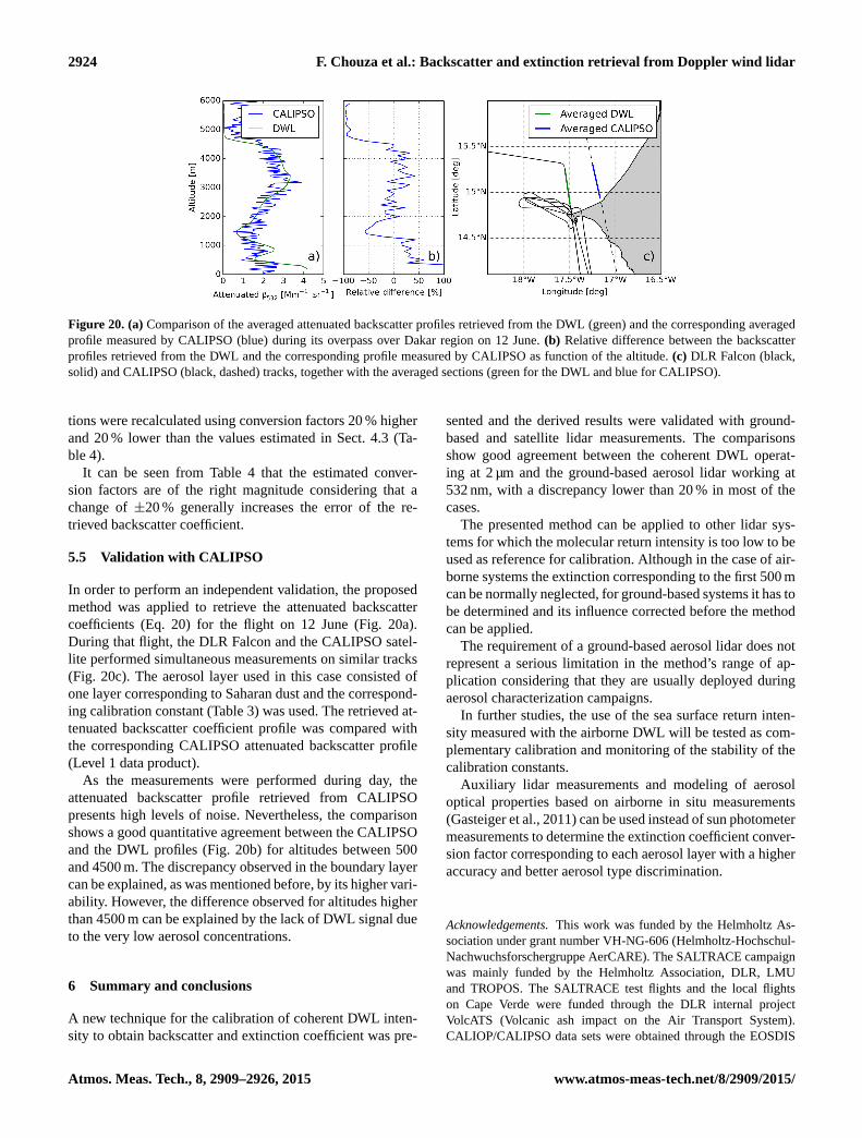
Figure 20. (a) Comparison of the averaged attenuated backscatter profiles retrieved from the DWL (green) and the corresponding averaged

profile measured by CALIPSO (blue) during its overpass over Dakar region on 12 June. (b) Relative difference between the backscatter

profiles retrieved from the DWL and the corresponding profile measured by CALIPSO as function of the altitude. (c) DLR Falcon (black,

solid) and CALIPSO (black, dashed) tracks, together with the averaged sections (green for the DWL and blue for CALIPSO).

tions were recalculated using conversion factors 20 % higher

and 20 % lower than the values estimated in Sect. 4.3 (Ta-

ble 4).

It can be seen from Table 4 that the estimated conver-

sion factors are of the right magnitude considering that a

change of ±20 % generally increases the error of the re-

trieved backscatter coefficient.

5.5 Validation with CALIPSO

In order to perform an independent validation, the proposed

method was applied to retrieve the attenuated backscatter

coefficients (Eq. 20) for the flight on 12 June (Fig. 20a).

During that flight, the DLR Falcon and the CALIPSO satel-

lite performed simultaneous measurements on similar tracks

(Fig. 20c). The aerosol layer used in this case consisted of

one layer corresponding to Saharan dust and the correspond-

ing calibration constant (Table 3) was used. The retrieved at-

tenuated backscatter coefficient profile was compared with

the corresponding CALIPSO attenuated backscatter profile

(Level 1 data product).

As the measurements were performed during day, the

attenuated backscatter profile retrieved from CALIPSO

presents high levels of noise. Nevertheless, the comparison

shows a good quantitative agreement between the CALIPSO

and the DWL profiles (Fig. 20b) for altitudes between 500

and 4500 m. The discrepancy observed in the boundary layer

can be explained, as was mentioned before, by its higher vari-

ability. However, the difference observed for altitudes higher

than 4500 m can be explained by the lack of DWL signal due

to the very low aerosol concentrations.

6 Summary and conclusions

A new technique for the calibration of coherent DWL inten-

sity to obtain backscatter and extinction coefficient was pre-

sented and the derived results were validated with ground-

based and satellite lidar measurements. The comparisons

show good agreement between the coherent DWL operat-

ing at 2 µm and the ground-based aerosol lidar working at

532 nm, with a discrepancy lower than 20 % in most of the

cases.

The presented method can be applied to other lidar sys-

tems for which the molecular return intensity is too low to be

used as reference for calibration. Although in the case of air-

borne systems the extinction corresponding to the first 500 m

can be normally neglected, for ground-based systems it has to

be determined and its influence corrected before the method

can be applied.

The requirement of a ground-based aerosol lidar does not

represent a serious limitation in the method’s range of ap-

plication considering that they are usually deployed during

aerosol characterization campaigns.

In further studies, the use of the sea surface return inten-

sity measured with the airborne DWL will be tested as com-

plementary calibration and monitoring of the stability of the

calibration constants.

Auxiliary lidar measurements and modeling of aerosol

optical properties based on airborne in situ measurements

(Gasteiger et al., 2011) can be used instead of sun photometer

measurements to determine the extinction coefficient conver-

sion factor corresponding to each aerosol layer with a higher

accuracy and better aerosol type discrimination.

Acknowledgements. This work was funded by the Helmholtz As-

sociation under grant number VH-NG-606 (Helmholtz-Hochschul-

Nachwuchsforschergruppe AerCARE). The SALTRACE campaign

was mainly funded by the Helmholtz Association, DLR, LMU

and TROPOS. The SALTRACE test flights and the local flights

on Cape Verde were funded through the DLR internal project

VolcATS (Volcanic ash impact on the Air Transport System).

CALIOP/CALIPSO data sets were obtained through the EOSDIS



website (https://earthdata.nasa.gov/). The sun photometer work

leading to these results has received funding from the European

Union Seventh Framework Programme (FP7/2007-2013) under

grant agreement nr. 262254 [ACTRIS]. We thank the AERONET

teams at GSFC, LOA and UVA for their support.

The article processing charges for this open-access

publication were covered by a Research

Centre of the Helmholtz Association.

Edited by: U. Wandinger

References

Ansmann, A. and Müller, D.: Lidar and Atmospheric Aerosol Par-

ticles, in: Lidar, edited by: Weitkamp, C., Springer, New York,

105–141, 2005.

Ansmann, A., Wandinger, U., Riebesell, M., Weitkamp, C., and

Michaelis, W.: Independent measurement of extinction and

backscatter profiles in cirrus clouds by using a combined Raman

elastic-backscatter lidar, Appl. Optics, 31, 7113–7113, 1992.

Ansmann, A., Petzold, A., Kandler, K., Tegen, I., Wendisch, M.,

Müller, D., Weinzierl, B., Müller, T., and Heintzenberg, J.: Sa-

haran Mineral Dust Experiments SAMUM-1 and SAMUM-2:

What have we learned?, Tellus B, 63, 403–429, 2011.

Böckmann, C., Wandinger, U., Ansmann, A., Bösenberg, J.,

Amiridis, V., Boselli, A., Delaval, A., De Tomasi, F., Frioud,

M., Grigorov, I., Hågård, A., Horvat, M., Iarlori, M., Komguem,

L., Kreipl, S., Larchevêque, G., Matthias, V., Papayannis, A.,

Pappalardo, G., Rocadenbosch, F., Rodrigues, J., Schneider, J.,

Shcherbakov, V., and Wiegner, M.: Aerosol lidar inter- compari-

son in the framework of the EARLINET project: Part II – Aerosol

backscatter algo- rithms, Appl. Optics, 43, 977–989, 2004.

Bou Karam, D., Flamant, C., Knippertz, P., Reitebuch, O., Pelon, J.,

Chong, M., and Dabas, A.: Dust emissions over the Sahel asso-

ciated with the West African monsoon intertropical discontinuity

region: A representative case-study, Q. J. Roy. Meteor. Soc., 134,

621–634, 2008.

Bufton, J. L., Hoge, F. E., and Swift, R. N.: Airborne measurements

of laser backscatter from the ocean surface, Appl. Optics, 22,

2603–2618, 1983.

Cutten, D. R., Rothermel, J., Jarzembski, M. A., Hardesty, R. M.,

Howell, J. N., Tratt, D. M., and Srivastava, V.: Radiometric cal-

ibration of an airborne CO2 pulsed Doppler lidar with a natural

earth surface, Appl. Optics, 41, 3530–3537, 2002.

Eck, T. F., Holben, B. N., Reid, J. S., Dubovik, O., Smirnov,

A., O’Neill, N. T., and Slutsker, I.: Wavelength dependence of

the optical depth of biomass burning, urban, and desert dust

aerosols, J. Geophys. Res., 104, 31333–31349, 1999.

Fernald, F. G.: Analysis of atmospheric lidar observations: some

comments, Appl. Optics, 23, 652–653, 1984.

Frehlich, R. G. and Kavaya, M. J.: Coherent laser radar performance

for general atmospheric refractive turbulence, Appl. Optics, 30,

5325–5352, 1991.

Freudenthaler, V., Esselborn, M., Wiegner, M., Heese, B., Tesche,

M., Ansmann, A., Müller, D., Althause, D., Wirth, M., Fix, A.,

Ehret, G., Knippertz, P., Toledano, C., Gasteiger, J., Garhammer,

M., and Seefeldner, M.: Depolarization ratio profiing at several

wavelengths in pure Saharan dust during SAMUM 2006, Tellus

B, 61, 165–179, 2009.

Freudenthaler, V., Seefeldner, M., Groß, S., and Wandinger, U.: Ac-

curacy of linear depolarisation ratios in clean air ranges measured

with POLIS-6 at 355 and 532 nm, Proceeding of 27. International

Laser Radar Conference, 5–10 July 2015, New York, 2015.

Gasteiger, J., Wiegner, M., Groß, S., Freudenthaler, V., Toledano,

C., Tesche, M., and Kandler, K.: Modelling lidar-relevant optical

properties of complex mineral dust aerosols, Tellus B, 63, 725–

741, 2011.

Groß, S., Esselborn, M., Weinzierl, B., Wirth, M., Fix, A., and Pet-

zold, A.: Aerosol classification by airborne high spectral reso-

lution lidar observations, Atmos. Chem. Phys., 13, 2487–2505,

doi:10.5194/acp-13-2487-2013, 2013.

Heintzenberg, J.: The SAMUM-1 experiment over Southern Mo-

rocco: Overview and introduction, Tellus Series B, 61, 2–11,

2009.

Henderson, S. W., Suni, P. J. M., Hale, C. P., Hannon, S. M., Magee,

J. R., Bruns, D. L., and Yuen, E. H.: Coherent laser radar at 2 µm

using solid-state lasers, IEEE T. Geosci. Remote, 31.1, 4–15,

doi:10.1109/36.210439, 1993.

Henderson, S. W., Gatt, P., Rees, D., and Huffaker, R. M.: Wind

Lidar, in: Laser Remote Sensing, edited by: Fujii, T. and Fukuchi,

T., CRC Press, Boca Raton, 469–722, 2005.

Hinds, W. C.: Aerosol Technology: Properties, Behaviour and Mea-

surement of Airborne Particles, John Wiley & Sons, Inc., New

York, 304–305, 1999.

Käsler, Y., Rahm, S., Simmet, R., and Kühn, M.: Wake measure-

ments of a multi-MW wind turbine with coherent long-range

pulsed doppler wind lidar, J. Atmos. Ocean. Tech., 27, 1529–

1532, 2010.

King, M. D. and Byrne, D. M.: A Method for Inferring Total Ozone

Content from the Spectral Variation of Total Optical Depth Ob-

tained with a Solar Radiometer, J. Atmos. Sci., 33, 2242–2251,

1976.

Klett, J. D.: Lidar inversion with variable backscatter/extinction ra-

tios, Appl. Optics, 24, 1638–1643, 1985.

Köpp, F., Rahm, S., and Smalikho, I.: Characterization of Aircraft

Wake Vortices by 2-µm Pulsed Doppler Lidar, J. Atmos. Ocean.

Tech., 21, 194–206, 2004.

Li, Z., Lemmerz, C., Paffrath, U., Reitebuch, O., and Witschas, B.:

Airborne Doppler Lidar Investigation of Sea Surface Reflectance

at a 355-nm Ultraviolet Wavelength, J. Atmos. Ocean. Tech., 27,

693–704, 2010.

Mahowald, N. M., Baker, A. R., Bergametti, G., Brooks, N., Duce,

R. A., Jickells, T. D., Kubilay, N., Prospero, J. M., and Tegen,

I.: Atmospheric global dust cycle and iron inputs to the ocean,

Global Biogeochem. Cy., 19, 1–15, 2005.

Menzies, R. T. and Tratt, D. M.: Airborne CO2 coherent lidar

for measurements of atmospheric aerosol and cloud backscat-

ter, Appl. Optics, 33, 5698–5711, 1994.

O’Connor, E. J., Illingworth, A. J., and Hogan, R. J.: A technique

for autocalibration of cloud lidar, J. Atmos. Ocean. Tech., 21,

777–786, 2004.

O’Neill, N. T., Eck, T. F., Reid, J. S., Smirnov, A., and Pancrati, O.:

Coarse mode optical information retrievable using ultraviolet to

short-wave infrared Sun photometry: Application to United Arab

Emirates Unified Aerosol Experiment data, J. Geophys. Res.,

113, D05212, doi:10.1029/2007JD009052, 2008.


https://earthdata.nasa.gov/

http://dx.doi.org/10.5194/acp-13-2487-2013

http://dx.doi.org/10.1109/36.210439

http://dx.doi.org/10.1029/2007JD009052


Prospero, J. M.: Long-range transport of mineral dust in the global

atmosphere: Impact of African dust on the environment of the

southeastern United States, P. Natl. Acad. Sci. USA., 96, 3396–

3403, 1999.

Reitebuch, O.: Wind Lidar for Atmospheric Research, in: Atmo-

spheric Physics, edited by: Schumann, U., Springer, Berlin Hei-

delberg, 487–507, 2012.

Reitebuch, O., Werner, C., Leike, I., Delville, P., Flamant, P. H.,

Cress, A., and Engelbart, D.: Experimental validation of wind

profiling performed by the airbone 10- µm heterodyne Doppler

Lidar WIND, J. Atmos. Ocean. Tech., 18, 1331–1344, 2001.

Schumann, U., Weinzierl, B., Reitebuch, O., Schlager, H., Minikin,

A., Forster, C., Baumann, R., Sailer, T., Graf, K., Mannstein, H.,

Voigt, C., Rahm, S., Simmet, R., Scheibe, M., Lichtenstern, M.,

Stock, P., Rüba, H., Schäuble, D., Tafferner, A., Rautenhaus, M.,

Gerz, T., Ziereis, H., Krautstrunk, M., Mallaun, C., Gayet, J.-

F., Lieke, K., Kandler, K., Ebert, M., Weinbruch, S., Stohl, A.,

Gasteiger, J., Groß, S., Freudenthaler, V., Wiegner, M., Ansmann,

A., Tesche, M., Olafsson, H., and Sturm, K.: Airborne observa-

tions of the Eyjafjalla volcano ash cloud over Europe during air

space closure in April and May 2010, Atmos. Chem. Phys., 11,

2245–2279, doi:10.5194/acp-11-2245-2011, 2011.

Seifert, P., Ansmann, A., Mattis, I., Wandinger, U., Tesche, M., En-

gelmann, R., Müller, D., Pérez, C., and Haustein, K.: Saharan

dust and heterogeneous ice formation: Eleven years of cloud ob-

servations at a central European EARLINET site, J. Geophys.

Res., 115, D20201, doi:10.1029/2009JD013222, 2010.

Smalikho, I.: Techniques of wind vector estimation from data mea-

sured with a scanning coherent Doppler Lidar, J. Atmos. Ocean.

Tech., 20, 276–291, 2003.

Sonnenschein, C. M. and Horrigan, F. A.: Signal-to-Noise Relation-

ships for Coaxial Systems that Heterodyne Backscatter from the

Atmosphere, Appl. Optics, 10, 1600–1604, 1971.

Toledano, C., Wiegner, M., Groß, S., Freudenthaler, V., Gasteiger,

J., Müller, D., Müller, T., Schladitz, A., Weinzierl, B., Torres, B.,

and O’Neill, N. T.: Optical properties of aerosol mixtures derived

from sun-sky radiometry during SAMUM-2, Tellus Series B, 63,

635–648, 2011.

Weinzierl, B., Sauer, D., Minikin, A., Reitebuch, O., Dahlkötter, F.,

Mayer, B., Emde, C., Tegen, I., Gasteiger, J., Petzold, A., Veira,

A., Kueppers, U., and Schumann, U.: On the visibility of air-

borne volcanic ash and mineral dust from the pilot’s perspective

in flight, J. Phys. Chem. Earth, 45, 87–102, 2012.

Weissmann, M., Busen, R., Dörnbrack, A., Rahm, S., and Reite-

buch, O.: Targeted observations with an airborne wind lidar, J.

Atmos. Ocean. Tech., 22, 1706–1719, 2005.


http://dx.doi.org/10.5194/acp-11-2245-2011

http://dx.doi.org/10.1029/2009JD013222

retrieval of aerosol backscatter and extinction from ... · pdf fileretrieval of aerosol...

Documents