laser surveying, topographic mapping, and … surveying, topographic mapping, and mapping ... laser...
TRANSCRIPT

TWO THIRDS RANGE (500-700 FT)
Laser Surveying, Topographic Mapping, and Mapping Drainage Systems using
GPS Designing Agricultural Systems to Balance Production and Environmental Objectives
Miscellaneous Bulletin OAWMGWG No. 1-2/2005
2005 Overholt Drainage School
March 7-11
Waterman Agricultural and Natural Resources Laboratory The Ohio State University
Columbus, Ohio
Sponsors and Partnerships
Overholt Drainage Education and Research Program
Department of Food, Agricultural,
and Biological Engineering
Ohio State University Extension
Ohio Agricultural Research and Development Center
College of Food, Agricultural, and
Environmental Sciences
The Ohio State University
USDA-Natural Resources Conservation Service (NRCS)
Ohio Land Improvement Contractors
Association (OLICA)
Ohio Department of Natural Resources
Ohio Agricultural Water Management
Guide Working Group
12/20/02 topocontour.ppt 2
You are Here

2005 OVERHOLT DRAINAGE SCHOOL SESSION I:
Laser Surveying Topographic Mapping
Mapping Drainage Systems using GPS
Monday, March 7
Waterman Agricutural and Natural Resources Laboratory
Columbus, Ohio
Presented by:
OVERHOLT DRAINAGE EDUCATION AND RESEARCH PROGRAM
Department of Food, Agricultural, and Biological Engineering
Ohio State University Extension Ohio Agricultural Research and Development Center
College of Food, Agricultural, and Environmental Sciences The Ohio State University
In Cooperation with:
USDA-Natural Resources Conservation Service
Ohio Land Improvement Contractors Association/Associates Ohio Department of Natural Resources Soil and Water Conservation Districts
USDA-Agricultural Research Service, Soil Drainage Research Unit Others
For information, additional copies of this manual, or suggestions, please contact
Dr. Larry C. Brown at 614.292.3826 or [email protected]
TABLE OF CONTENTS 2005 Overholt Drainage School
Session I Laser Surveying, Topographic Mapping, Mapping Drainage Systems using GPS
INTRODUCTION Page
2005 Session 1 Program Overholt Drainage Education and Research Program, Drainage Hall of Fame
LASER SURVEYING
Laser Surveying - PowerPoint Presentation notes Checking Transmitter for Accuracy -PowerPoint Pres notes Direct Elevation Surveying Work Sheet
LASER MANUAL
TOPOGRAPHIC MAPPING
Topographic Information - PowerPoint Presentation notes USGS Map Information and Symbols
DRAWING CONTOURS
Contour Exercises - PowerPoint Presentation notes Profiles and EARTHWORK INFORMATION
Profiles from a Topographic Map - PowerPoint Presentation notes Units of Measurement for Earthwork Conversion from Inches to Feet Mapping Scale Conversions Factors Affecting Job Cost Estimates
GPS AND MAPPING
GPS Simplified Fact Sheet GPS Guidance Systems: Tips for Purchasing a System Fact Sheet Understanding GPS Accuracy for Agricultural Applications Fact Sheet HANDOUT MATERIAL End

Tab for Introduction

2005 Overholt Drainage School Session 1
Laser Surveying (Leveling), Topographic Mapping and Mapping Drainage Systems using GPS
Monday, March 7 – 8:30 AM to 9:00 PM MORNING Moderator: Larry C. Brown 8:00-8:30 Check-in, Main Meeting Room, Waterman Agricultural and Natural
Resources Laboratory, The Ohio State University, Columbus, Ohio 8:45 School begins, Welcome, Introduction, Instructors, Notebook, etc.
(Brown) Instructors: Ron Cornwell, Rick Galehouse, Fred Galehouse, Paul DeMuth Louis McFarland, Mark Seger, others ♦ Introduction to Lenker Rod ♦ Field Notes with Lenker Rod ♦ Principles of Laser Surveying ♦ Rod Readings and Notes for Leveling with Laser ♦ Completing Turning Points and Field Notes ♦ Assignment of Teams and Instructors (Brown) Break ♦ Field Exercises at Waterman Lab ♦ Application of Laser Leveling to Topographic Mapping ♦ Waterman Lab Field Problem - Laser Surveying for Drainage Design (Brown) LUNCH At Waterman Lab Office Building AFTERNOON Moderator and Field Leaders: McFarland//Larry Brown Team Leaders: Fred Galehouse, Rick Galehouse, Paul Chester, Mark Seger, Louis McFarland, Paul DeMuth, Nathan Davis, Bruce Atherton, Nick Miller, others ♦ Review of Field Problem and Topographic Mapping ♦ Walk to Field Site, Begin Field Survey Problem to completion (15+ ac, 100’ grid) ♦ Return to Waterman Lab ♦ Review of Field Problem (Cornwell/McFarland/Brown) ♦ Features of Topographic Maps (Seger) ♦ Review of Drawing Contours (Seger/Galehouses/others) SUPPER Own Your Own PLEASE BE BACK BY 6:30 PM sharp.

2005 Overholt Drainage School Laser Surveying (Leveling), Topographic Mapping and Mapping Drainage
Systems using GPS Monday, March 7 – Continued
EVENING 6:30–9:00 PM Moderator: Larry Brown Instructors: Mark Seger, Fred Galehouse, Rick Galehouse, Ron Cornwell, Louis
McFarland, Paul DeMuth, and team leaders ♦ Plotting Waterman Field Data (team leaders working with students) ♦ Drawing Contour Map from Plotted Field Data (team leaders working with students) ♦ Completed Topographic Map of Field Problem ♦ Applications - as Time Allows:
• Profile information from topographic map • Slope, grade, earthwork information from topographic map
♦ Wrap-up, evaluation, review of Monday’s and Tuesday’s program (Brown) 9:00 PM Evening Ends – Program Continues Tuesday Morning at 8:00 AM SHARP - sleep well
Tuesday, March 8 – 8:00 AM to 12:00 PM Laser Surveying (Leveling), Topographic Mapping and Mapping Drainage
Systems using GPS MORNING Moderator: Larry C. Brown 8:00-8:30 Review of Monday’s Program and Accomplishments (Brown and
other Instructors) Overview of Tuesday Morning Program (Brown) Instructors: Larry Brown, Nick Miller, William Northcott, Eric Schuler, others ♦ Overview and Demonstration of Computer Applications for Drawing Contours ♦ GPS Introduction ♦ GPS Applications and Drainage System Mapping ♦ GPS Mapping Demonstration ♦ Group Q/A, Discussion Noon End Session 1, Wrap-up, evaluation, review of Tuesday’s program (Brown)
Box LUNCH At Waterman Lab Office Building, and transition to Session 2, Subsurface Drainage Design

VIRGIL OVERHOLT DRAINAGE EDUCATION AND RESEARCH PROGRAM
in the Department of Food, Agricultural, and Biological Engineering
College of Food, Agricultural, and Environmental Sciences THE OHIO STATE UNIVERSITY
Columbus, Ohio March 15, 2005
Dr. Larry C. Brown, Professor and Executive Director
International Program for Water Management in Agriculture
Introduction The program is named in honor of the late Professor Virgil Overholt, who devoted 42 years to education and research on agricultural drainage in Ohio. It also recognizes the outstanding contributions of Ohio industry through the development of drainage materials and equipment. Ohio continues to be a world leader in agricultural drainage and land improvement. Two of the largest corrugated plastic-tubing manufacturers in the nation have their corporate offices and research laboratories in Ohio. The world's largest producer of grade-control equipment for earth-moving machines, two major trencher manufacturers, and several large concrete and clay tile plants are also located in the state. A drainage contractors’ school has been held annually for 40 years and an active drainage research program has been underway for more than 41 years. Ohio leads the nation in the installation of underground agricultural drains. Also, the USDA Agricultural Research Service Soil Drainage Research Unit is housed in the Department of Food, Agricultural, and Biological Engineering, and has been an integral part of the Department's soil and water program for many years. For these and other reasons, the proposed national water management laboratory for humid agricultural lands is planned for Columbus. Such activity indicates that the state has been and should continue to be a leader in agricultural drainage. The Overholt Drainage Education and Research Program, which includes the International Drainage Hall of Fame Award and the Drainage Design School, is now part of the International Program for Water Management in Agriculture. This program, initiated in 1984, is an outgrowth of nearly 60 years of drainage education and research at The Ohio State University by eminent scholars and educators, such as Virgil Overholt, Mel Palmer, Glenn Schwab, and Byron Nolte.
Program Objectives The program has three major objectives:
1. To recognize outstanding educators, researchers, contractors, farmers, and/or industrialists who have made significant contributions to the development and use of drainage in agricultural production.
2. To conduct continuing education and outreach education programs in drainage engineering and technology through annual in-depth schools for teachers, researchers, contractors, technicians, industry personnel, and engineers in private or public practice.

3. To conduct drainage research programs to meet current and future needs including: crop response, timeliness of tillage and harvesting, economics, environmental impacts and remediation, and other management factors influencing the installation and operation of agricultural drainage systems.
International Drainage Hall of Fame
Dedicated to Virgil Overholt (1889-1978) The "Drainage Hall of Fame" was established in the Agricultural Engineering Department at The Ohio State University in 1979. It is dedicated to Virgil Overholt, Professor of Agricultural Engineering (1915-1956) for 42 years of outstanding service in education and research on agricultural drainage. The Drainage Hall of Fame at The Ohio State University was dedicated to the memory of Virgil Overholt on March 9, 1979.
Recognition of Professor Overholt
Superior Service Award, USDA, 1956 John Deere Medal, American Society of Agricultural Engineers, 1961
Ohio Agricultural Hall of Fame, 1969 Distinguished Service Award, OSU, 1971
Honorary Life Member, Ohio Land Improvement Contractor's Association Registered Professional Engineer
American Society of Agricultural Engineers, Chair, Soil & Water Division Soil Conservation Society of America, Member
Ohio State University Council, Member Extension Professors Association, Member
Gamma Sigma Delta, President, Ohio Chapter Evangelical-United Brethren Church, Chair, Board of Trustees
Professor Overholt's outstanding achievement was the 42 years which he spent as a teaching and extension specialist in Agricultural Engineering at The Ohio State University. He was a gentle and sensitive person with high regard for his fellow man. His keen interest in people and helping solve their problems was one of his outstanding abilities. His specialty was agricultural drainage and other related soil and water conservation problems. He developed many charts and mimeographed materials for making sound recommendations prior to development of present standards. He was one of the leaders in this field of work. In Ohio he was commonly referred to as "Mr. Drainage," and was highly regarded by his students, his colleagues, and farmers throughout the state. Throughout his career he developed a keen sense of observation and an outstanding ability to remember names, places, and events. Starting in 1979, an annual Hall of Fame award has been given to an outstanding person who has made significant contributions to the development and use of drainage in agricultural production for an extended period of time. The Drainage Hall of Fame Award, in honor of Virgil Overholt, has international scope. Persons eligible for nomination include those who have provided extensive service to the science, art, engineering, and/or practice of agricultural drainage and water management in any of the following areas: teaching, extension education, research, technology development, consulting, contractor training, implementation and practice, leadership in the agricultural drainage

industry at the state or national level, etc. Nominations are due before October 1 of each year for that year's award. Each nomination is considered for a total period of three years before a new nomination form must be submitted. Forms and instructions are available from the Executive Director of the International Program for Water Management in Agriculture, The Ohio State University.
Previous Honorees
Don Kirkham – 1979 Jan van Schilfgaarde - 1980
James N. Luthin - 1981 Fred H. Galehouse - 1982 Glenn O. Schwab - 1983 R. Wayne Skaggs - 1984 Brian D. Trafford - 1985
Marion M. Weaver - 1986 Jans Wesseling - 1987
Melville L. Palmer - 1988 Ray J. Winger, Jr. - 1989 James L. Fouss - 1990
William W. Donnan - 1991 Ted L. Teach - 1992
Robert S. Broughton - 1993 Wiebe H. van der Molen - 1994
Lyman S. Willardson - 1995 Walter J. Ochs – 1996
Carroll J.W. Drablos – 1997 Gordon Spoor – 1998
1999 - No Award Ronald C. Reeve – 2000
2001 – No Award 2002 – Norman R. Fausey
Note: Nominations must be received by October 1 to be considered for that year. A Jury is selected, and the award announced in January or March, the following year.
Overholt Drainage School A drainage school is held each year, usually in Columbus. Since 1999, the school has been held at different locations around the state. Topics range from drainage and subirrigation design, basic and laser surveying for soil and water conservation, and specialty topics in water management. Highly competent, experienced drainage and water management experts help organize and conduct the school. The drainage school is open to participants from any state and country on a first-come basis. Pre-registration is necessary as enrollment is limited to the number that can be accommodated for a quality educational program. School dates are usually announced in advance, i.e., the 2006 school is tentatively scheduled for the week of March 13 (location yet to be determined). A registration fee is charged for books and supplies, and other school related expenses. Interest from the endowments and contributions to the program defray a portion of the costs.
Drainage Research The program supplements an on-going research effort in cooperation with the U.S. Department of Agriculture and the Ohio Agricultural Research and Development Center. Training of young engineers and scientists, and the support of plot-scale and long-term field research, and computer modeling are emphasized. The collection of reliable data for evaluating the economics and environmental impact of agricultural drainage, water table management with controlled drainage and subirrigation, drainage water management, and performance of drainage installation equipment have major emphasis.

Advisory Group
An advisory committee provides advice and suggestions for program direction, and selects the jury for the Drainage Hall of Fame Award. Committee membership includes: a representative from each Overholt Club contributor; the Ohio Land Improvement Contractors Association; the USDA Soil Conservation Service (Ohio); the Ohio Department of Natural Resources; and the Ohio Section, American Society of Agricultural Engineers, as well as faculty members from the Agricultural Engineering Department at The Ohio State University, and The Land Improvement Contractors of America. Members may be selected from other organizations.
Program Support Contributions to the program should be made payable to The Ohio State University Development Fund and designated to the Overholt Drainage Education and Research Program. Contributions are tax deductible. Recognition of contributors is as follows:
Overholt Club Member - $10,000 or more Gold Sponsor - $5,000 to 9,999; Silver Sponsor - $500 to 4,999; Bronze Sponsor -
$100 to 499
Contributors (Updated listing will be released Fall of 2005)
The Program Proudly Recognizes and Thanks Its Supporters
For more information about the program, email, write or phone:
Dr. Larry C. Brown, Professor and Executive Director Overholt Drainage Education and Research Program
International Program for Water Management in Agriculture Department of Food, Agricultural, and Biological Engineering
The Ohio State University 590 Woody Hayes Drive
Columbus, Ohio 43210-1057 Phone: 614.292.3826 FAX: 614.292.9448 [email protected]

Tab for laser Surveying
Slide 1
01/12/05 LASER SURVEYING V4 1
LASER SURVEYING
Ohio Land Improvement Contractors Association
Ron Cornwell, Paul Demuth, Fred & Rick GalehouseLouis McFarland
________________________________
________________________________
________________________________
Slide 2
01/12/05 LASER SURVEYING V4 2
Objectives
Introduce parts of a Laser Surveying System. Properly set up and use the system to produce
usable information (Elevations).
________________________________
________________________________
________________________________
Slide 3
01/12/05 LASER SURVEYING V4 3
Got Some Questions?
There is a lot of information in this course and we will be proceeding rather quickly.
If you have questions along the way please ask them.
There are no stupid questions.
________________________________
________________________________
________________________________
Slide 4
01/12/05 LASER SURVEYING V4 4
LASER Acronym
L - is for LightA - is for Amplification byS - is for Stimulated E - is for Emission ofR - is for Radiation
_______________________________
_______________________________
_______________________________
Slide 5
01/12/05 LASER SURVEYING V4 5
Parts of a Laser Surveying System
Laser Transmitter with tripod or mounting.
Level Rod (Conventional or Lenker Rod).
Rod Receiver (Laser light receiver on Level Rod).
Field book to record information
________________________________
________________________________
________________________________
Slide 6
01/12/05 LASER SURVEYING V4 6
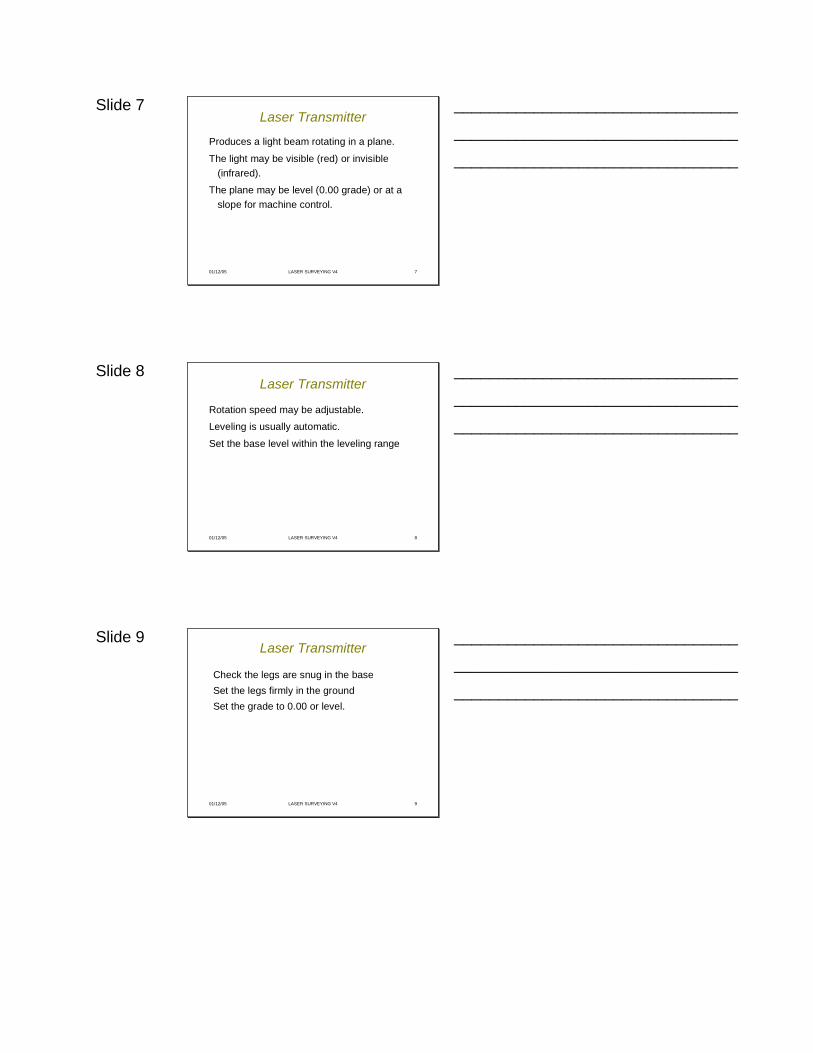
Laser Transmitter
Sometimes called the Command Post with tripod or mounting.May have external battery
________________________________
________________________________
________________________________
Slide 7
01/12/05 LASER SURVEYING V4 7
Laser Transmitter
Produces a light beam rotating in a plane.
The light may be visible (red) or invisible (infrared).
The plane may be level (0.00 grade) or at a slope for machine control.
________________________________
________________________________
________________________________
Slide 8
01/12/05 LASER SURVEYING V4 8
Laser Transmitter
Rotation speed may be adjustable.
Leveling is usually automatic.
Set the base level within the leveling range
________________________________
________________________________
________________________________
Slide 9
01/12/05 LASER SURVEYING V4 9
Laser Transmitter
Check the legs are snug in the baseSet the legs firmly in the ground Set the grade to 0.00 or level.
________________________________
________________________________
________________________________
Slide 10
01/12/05 LASER SURVEYING V4 10
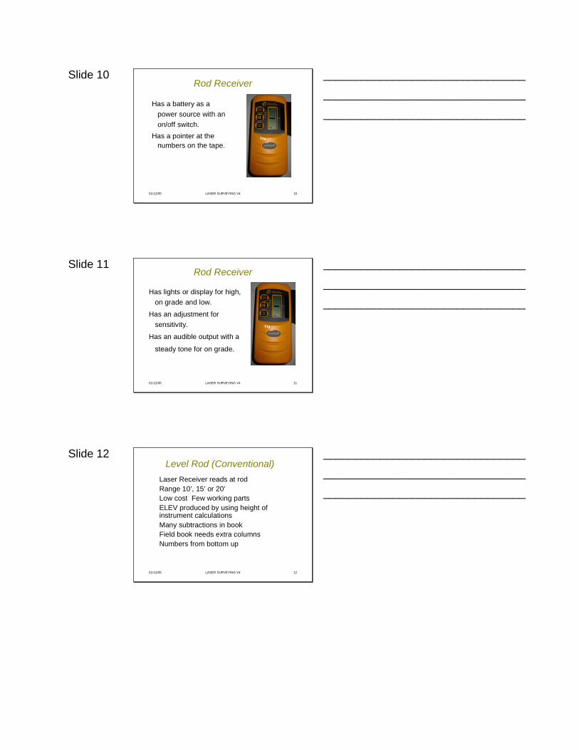
Rod Receiver
Has a battery as a power source with an on/off switch.
Has a pointer at the numbers on the tape.
________________________________
________________________________
________________________________
Slide 11
01/12/05 LASER SURVEYING V4 11
Rod Receiver
Has lights or display for high, on grade and low.
Has an adjustment for sensitivity.
Has an audible output with a
steady tone for on grade.
________________________________
________________________________
________________________________
Slide 12
01/12/05 LASER SURVEYING V4 12
Level Rod (Conventional)Laser Receiver reads at rod Range 10’, 15’ or 20’Low cost Few working partsELEV produced by using height of instrument calculationsMany subtractions in bookField book needs extra columnsNumbers from bottom up
________________________________
________________________________
________________________________
Slide 13
01/12/05 LASER SURVEYING V4 13
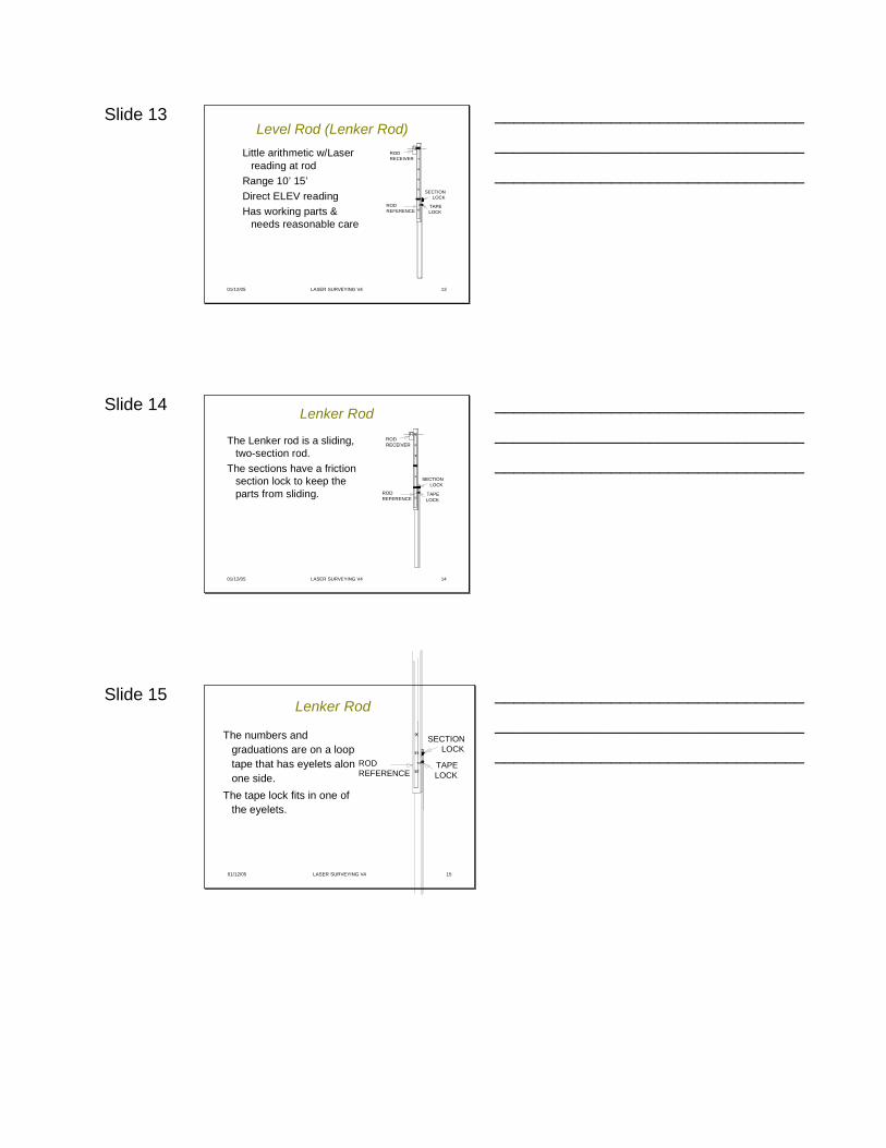
Level Rod (Lenker Rod)Little arithmetic w/Laser
reading at rod Range 10’ 15’Direct ELEV readingHas working parts &
needs reasonable care
RODREFERENCE
TAPELOCK
ROD RECEIVER
9
12
X
11
7
8
6
SECTIONLOCK
________________________________
________________________________
________________________________
Slide 14
01/12/05 LASER SURVEYING V4 14
Lenker Rod
The Lenker rod is a sliding, two-section rod.
The sections have a friction section lock to keep the parts from sliding. ROD
REFERENCETAPELOCK
ROD RECEIVER
9
12
X
11
7
8
6
SECTIONLOCK
________________________________
________________________________
________________________________
Slide 15
01/12/05 LASER SURVEYING V4 15
Lenker Rod
The numbers and graduations are on a loop tape that has eyelets along one side.
The tape lock fits in one of the eyelets.
RODREFERENCE
TAPELOCK12
X
11
SECTIONLOCK
________________________________
________________________________
________________________________
Slide 16
01/12/05 LASER SURVEYING V4 16
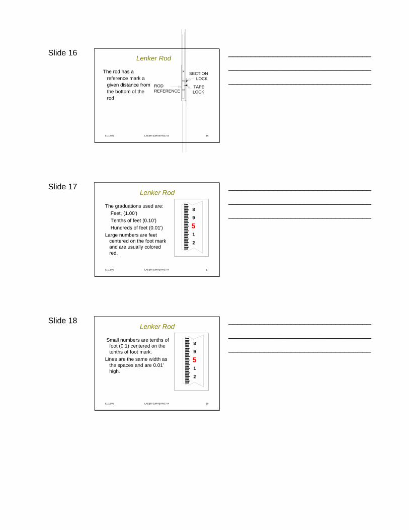
Lenker Rod
The rod has a reference mark a given distance from the bottom of the rod
RODREFERENCE
TAPELOCK12
X
11
SECTIONLOCK
________________________________
________________________________
________________________________
Slide 17
01/12/05 LASER SURVEYING V4 17
Lenker Rod
The graduations used are:Feet, (1.00') Tenths of feet (0.10') Hundreds of feet (0.01')
Large numbers are feet centered on the foot mark and are usually colored red.
8
9
51
2
________________________________
________________________________
________________________________
Slide 18
01/12/05 LASER SURVEYING V4 18
Lenker Rod
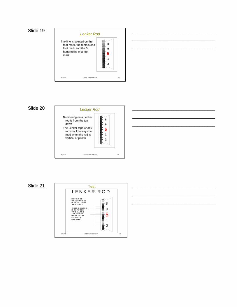
Small numbers are tenths of foot (0.1) centered on the tenths of foot mark.
Lines are the same width as the spaces and are 0.01' high.
8
9
51
2
________________________________
________________________________
________________________________
Slide 19
01/12/05 LASER SURVEYING V4 19
Lenker Rod
The line is pointed on the foot mark, the tenth’s of a foot mark and the 5 hundredths of a foot mark.
8
9
51
2
________________________________
________________________________
________________________________
Slide 20
01/12/05 LASER SURVEYING V4 20
Lenker Rod
Numbering on a Lenker rod is from the top down
The Lenker tape or any rod should always be read when the rod is vertical or plumb
8
9
51
2
________________________________
________________________________
________________________________
Slide 21
01/12/05 LASER SURVEYING V4 21
L E N K E R R O DN O T E : R O D G R A D U A T IO N S IN F E E T , 1 0 th s , A N D 1 0 0 th s
W H E N P O IN T E R IS B E T W E E N T W O M A R K S T H E L O W E R M A R K IS T H E C O R R E C T R E A D IN G
89
12
5
Test
________________________________
________________________________
________________________________
Slide 22
01/12/05 LASER SURVEYING V4 22
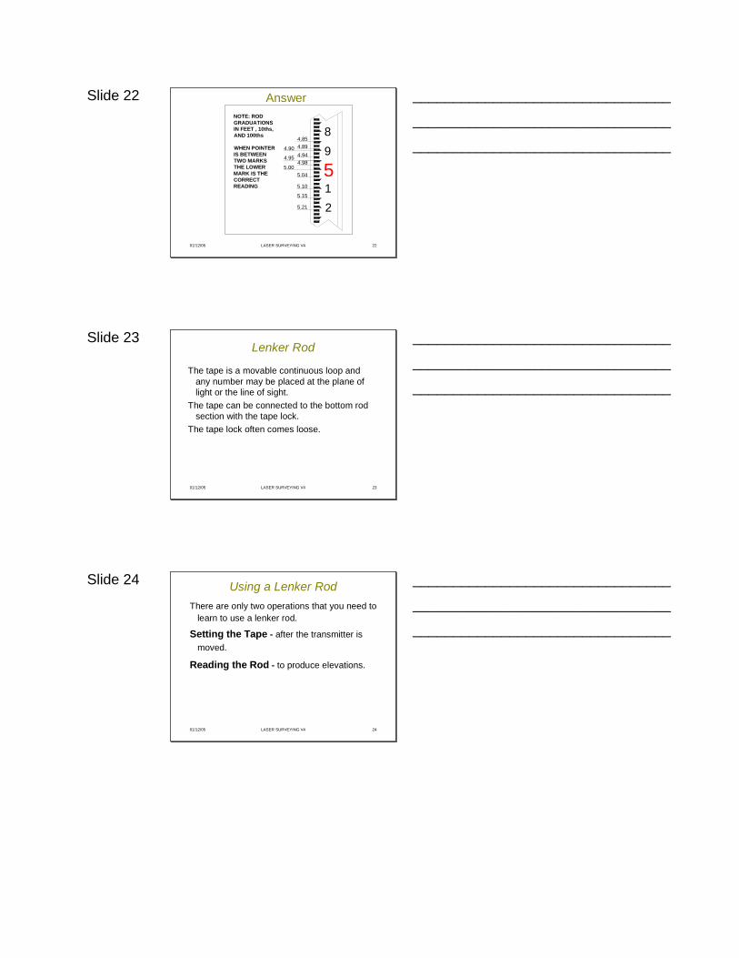
AnswerNOTE: ROD GRADUATIONS IN FEET , 10ths, AND 100ths
WHEN POINTER IS BETWEEN TWO MARKS THE LOWER MARK IS THE CORRECT READING
5.04
5.21
5.15
5.10
4.984.944.894.85
5.00
4.95
4.90
89
12
5
________________________________
________________________________
________________________________
Slide 23
01/12/05 LASER SURVEYING V4 23
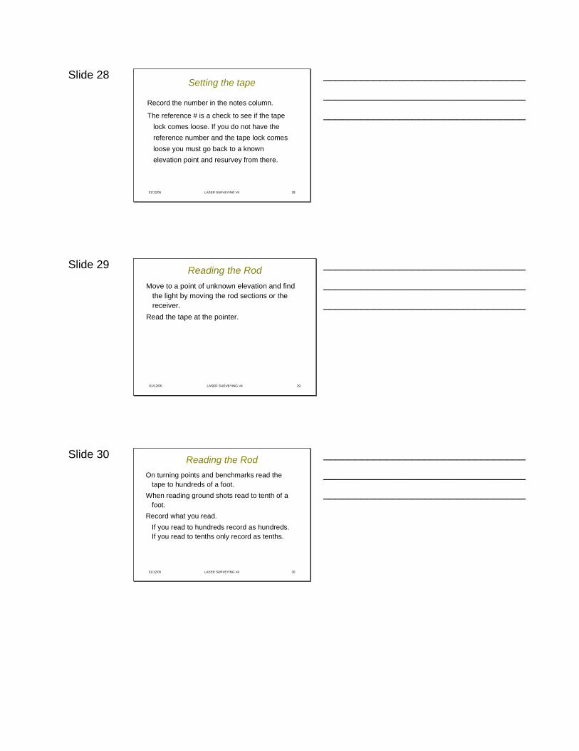
Lenker Rod
The tape is a movable continuous loop and any number may be placed at the plane of light or the line of sight.
The tape can be connected to the bottom rod section with the tape lock.
The tape lock often comes loose.
________________________________
________________________________
________________________________
Slide 24
01/12/05 LASER SURVEYING V4 24
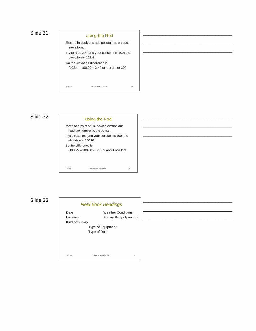
Using a Lenker RodThere are only two operations that you need to
learn to use a lenker rod.
Setting the Tape - after the transmitter is moved.
Reading the Rod - to produce elevations.
________________________________
________________________________
________________________________

Slide 25
01/12/05 LASER SURVEYING V4 25
Setting the Tape
Find the light.
Lock or hold the rod sections together.
Move the tape so the elevation (ft, tenths, hundreds) is at the receiver pointer.
________________________________
________________________________
________________________________
Slide 26
01/12/05 LASER SURVEYING V4 26
Setting the tape
Use a number that represents a known elevation (BM or TP).
If the elevation is 100.00 set the tape at 0
(also reads 10) and (100 becomes your
constant).
________________________________
________________________________
________________________________
Slide 27
01/12/05 LASER SURVEYING V4 27
Setting the tape
Set the tape lock in one of the holes and tighten the lock screw.
Check the setting and adjust if not correct.
Follow the reference point around the rod and read the tape.
________________________________
________________________________
________________________________
Slide 28
01/12/05 LASER SURVEYING V4 28
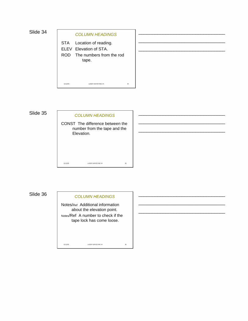
Setting the tape
Record the number in the notes column.
The reference # is a check to see if the tape lock comes loose. If you do not have the reference number and the tape lock comes loose you must go back to a known elevation point and resurvey from there.
________________________________
________________________________
________________________________
Slide 29
01/12/05 LASER SURVEYING V4 29
Reading the RodMove to a point of unknown elevation and find
the light by moving the rod sections or the receiver.
Read the tape at the pointer.
________________________________
________________________________
________________________________
Slide 30
01/12/05 LASER SURVEYING V4 30
Reading the RodOn turning points and benchmarks read the
tape to hundreds of a foot.When reading ground shots read to tenth of a
foot.Record what you read.
If you read to hundreds record as hundreds. If you read to tenths only record as tenths.
________________________________
________________________________
________________________________
Slide 31
01/12/05 LASER SURVEYING V4 31
Using the RodRecord in book and add constant to produce
elevations.
If you read 2.4 (and your constant is 100) the elevation is 102.4
So the elevation difference is (102.4 – 100.00 = 2.4’) or just under 30”
________________________________
________________________________
________________________________
Slide 32
01/12/05 LASER SURVEYING V4 32
Using the RodMove to a point of unknown elevation and
read the number at the pointer.
If you read .95 (and your constant is 100) the elevation is 100.95
So the difference is (100.95 – 100.00 = .95’) or about one foot
________________________________
________________________________
________________________________
Slide 33
01/12/05 LASER SURVEYING V4 33
Field Book Headings
Date Weather ConditionsLocation Survey Party (1person)Kind of Survey
Type of EquipmentType of Rod
________________________________
________________________________
________________________________
Slide 34
01/12/05 LASER SURVEYING V4 34
COLUMN HEADINGS
STA Location of reading.ELEV Elevation of STA.ROD The numbers from the rod
tape.
________________________________
________________________________
________________________________
Slide 35
01/12/05 LASER SURVEYING V4 35
COLUMN HEADINGS
CONST The difference between the number from the tape and the Elevation.
________________________________
________________________________
________________________________
Slide 36
01/12/05 LASER SURVEYING V4 36
COLUMN HEADINGS
Notes/Ref Additional information about the elevation point.
Notes/Ref A number to check if the tape lock has come loose.
________________________________
________________________________
________________________________
Slide 37
01/12/05 LASER SURVEYING V4 37
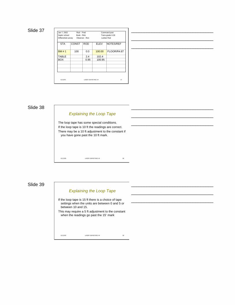
100.950.95BOX102.42.4 TABLE
FLOOR/R4.87100.000.0100 BM # 1
NOTES/REFELEVRODCONSTSTA
Jan 7, 2002 Rod – Fred Command postSeptic school Book - Rick Trans grade 0.00Differential survey Observer - Ron Lenker Rod
________________________________
________________________________
________________________________
Slide 38
01/12/05 LASER SURVEYING V4 38
Explaining the Loop Tape
The loop tape has some special conditions.If the loop tape is 10 ft the readings are correct.There may be a 10 ft adjustment to the constant if
you have gone past the 10 ft mark.
________________________________
________________________________
________________________________
Slide 39
01/12/05 LASER SURVEYING V4 39
Explaining the Loop Tape
If the loop tape is 15 ft there is a choice of tape settings when the units are between 0 and 5 or between 10 and 15.
This may require a 5 ft adjustment to the constant when the readings go past the 15’ mark
________________________________
________________________________
________________________________

Slide 40
01/12/05 LASER SURVEYING V4 40
A Helpful Rule Reducing the Number of Adjustments Needed
When elevations are below the known elevation, select the higher or 10 to 15 range.
________________________________
________________________________
________________________________
Slide 41
01/12/05 LASER SURVEYING V4 41
Are there any questions ?
________________________________
________________________________
________________________________
Slide 1
01/09/04 CHECKING THE TRANSMITTER V1 1
CHECKING THE TRANSMITTER
Ohio Land Improvement Contractors Association
Fred & Rick GalehouseRon CornwellPaul Demuth
________________________________
________________________________
________________________________
Slide 2
01/09/04 CHECKING THE TRANSMITTER V1 2
Checking the Transmitter
________________________________
________________________________
________________________________
Slide 3
01/09/04 CHECKING THE TRANSMITTER V1 3
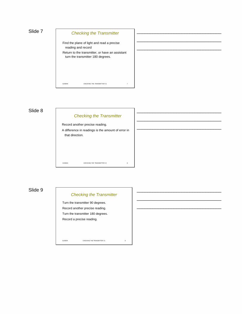
Checking the Transmitter
Check legs are snug in the base Set the base very level.Set the tripod firmly. Set the grade to 0.00 or level.
________________________________
________________________________
________________________________
Slide 4
01/09/04 CHECKING THE TRANSMITTER V1 4
Checking the Transmitter
Go to a solid point about two thirds the range of the transmitter.
Aim one of the grade directions at the point.
________________________________
________________________________
________________________________
Slide 5
01/09/04 CHECKING THE TRANSMITTER V1 5
Checking the Transmitter
T W O T H IR D S R A N G E (50 0-700 FT )
________________________________
________________________________
________________________________
Slide 6
01/09/04 CHECKING THE TRANSMITTER V1 6
Checking the Transmitter
A precise reading is one with the sensitivity at the finest setting and the rod held very vertical.
You may want to average several readings
________________________________
________________________________
________________________________
Slide 7
01/09/04 CHECKING THE TRANSMITTER V1 7
Checking the Transmitter
Find the plane of light and read a precise reading and record
Return to the transmitter, or have an assistant turn the transmitter 180 degrees.
________________________________
________________________________
________________________________
Slide 8
01/09/04 CHECKING THE TRANSMITTER V1 8
Checking the Transmitter
Record another precise reading.
A difference in readings is the amount of error in that direction.
________________________________
________________________________
________________________________
Slide 9
01/09/04 CHECKING THE TRANSMITTER V1 9
Checking the Transmitter
Turn the transmitter 90 degrees.
Record another precise reading.
Turn the transmitter 180 degrees.
Record a precise reading.
________________________________
________________________________
________________________________

Slide 10
01/09/04 CHECKING THE TRANSMITTER V1 10
Checking the Transmitter
A difference in readings is the amount of error in that direction.
If the amount is small or “0” you will have confidence in the accuracy of the transmitter
________________________________
________________________________
________________________________
Slide 11
01/09/04 CHECKING THE TRANSMITTER V1 11
Checking the Transmitter
If the readings recorded are different, this indicates an error in the transmitter and the transmitter should be serviced .
A dual slope transmitter could have an error if both grades are not set level.
________________________________
________________________________
________________________________
Slide 12
01/09/04 CHECKING THE TRANSMITTER V1 12
Are there any questions ?
________________________________
________________________________
________________________________

Station
Constant
Rod Reading
Elevation
Notes

Tab for Laser Manual

Galehouse Laser Surveying Manual
Preface
This manual is a labor of love by Mr. Fred H. Galehouse, Doylestown, Ohio. Fred originally developed this manual for laser surveying educational sessions taught at the Overholt Drainage School, as part of the Virgil Overholt Drainage Education and Research Program at The Ohio State University. The development of this manual was guided by Fred, and since 1989 it has evolved through his continued contributions and dedication, and from suggestions, recommendations, refinements by many people, the least of which is Fred’s son Rick (co-author, illustrator, etc.). The current version is a portion of the original written by Fred in 1989. The following is the verbatim 1989 Preface.
This manual was prepared for the laser surveying school of the Virgil Overholt Drainage Education and Research Program, at The Ohio State University.
Most of the manuals I have seen treat laser surveying as a new method and do not interface with basic surveying procedures. In this manual I have tried to provide this connection and in the process show the advantage of advances in use of the lenker rod, laser surveying and machine control. The rod usage illustrated in this manual is a lenker rod. In the writing of this manual I wish to thank all of the people and companies that have provided information, manuals and ideas. Without their cooperation, this manual would have been impossible. The following provided manuals from which both pictures and text have been copied; Ontario Ministry of Agriculture and Food – Contractors Short Course, Spectra –Physics-Laserplane, Rome - By-Linear Laser Systems, Control Instruments Inc. and Soil Conservation Service. Individuals who have also helped with encouragement and information are Mel Palmer, Glenn Schwab, and Byron Nolte of Ohio State University; John Johnston and Jim Myslik, Ontario Ministry of Agriculture and Food; Joe Harrington and Bob Burris of the U.S. Soil Conservation Service; Ron Cornwell and Tom Dew – Contractors; and my son Rick who is a co-author. There are many others who have provided encouragement and information and to all of which I say “thanks”.
I would be the first one to say that it is not complete and will probably never be completely up to date as there are new advances and changes, constantly. I just recently realized there are no references to lenker rod usage in Soil Conservation Service Field manuals. I would appreciate any comments on omissions and improvements that would enable an update. The manual is written for subsurface drainage only, due to time constraints. Some other manuals are excellent in their coverage of land grading.
Thanks to all of you who have helped. Fred Galehouse, March 1989
Fred has continued to provide this material for the Drainage School since 1989, and each year presents revisions and enhancements, with the help of his son Rick. The Overholt Drainage School instructors, including Fred, have used the various revisions of this manual in 13 Drainage Schools since 1989 (1989-1992; 1994; 1996-1998; 2000-2001; 2003-2005), helping to educate over 550 land improvement contractors, farmers, consultants, and others. Fred, the first and only land improvement contractor voted to the International Drainage Hall of Fame continues to donate the use of his manual to the Overholt Drainage Education and Research Program to help advance the knowledge and skills of land improvement contractors worldwide. We thank Fred Galehouse for his continued contributions to the profession of land improvement. Dr. Larry C. Brown, The Ohio State University; [email protected]
LASER MANUAL
BY FRED GALEHOUSE
1989

PREFACE
This manual was prepared for the laser surveying school of the Virgil Overholt Drainage Education and Research Program, at The Ohio State University. Most of the laser manuals I have seen treat laser surveying as a new method and do not interface with basic surveying procedures. In this manual I have tried to provide this connection and in the process show the advantage of advances in use of a Lenker rod, laser surveying and machine control. The rod usage illustrated in this manual is a Lenker rod. In the writing of this manual I wish to thank all of the people and companies that have provided information, manuals and ideas. Without this cooperation, this manual would have been impossible. The following provided manuals form which both pictures and text have been copied: Ontario Ministry of Agriculture and Food – Contractors Short Course. Spectra – Physics – Laserplane, Rome – By –Linear Laser Systems, Control Instruments Inc. and Soil Conservation Service. Individuals who have also helped with encouragement and information are Mel Palmer, Glenn Schwab, Byron Nolte of Ohio State University; John Johnson and Jim Myslik of Ontario Ministry of Agriculture and Food; Joe Harrington and Bob Burris of the U.S. Soil Conservation Service; Ron Cornwell and Tom Dew – OLICA contractors; and my son Rick who is a co-author. There are many others who have provided encouragement and information and to all of which I say “Thanks”. I would be the first one to say it is not complete and will probably never be completely up to date as there are new advances and changes constantly. I just recently realized there are no references to Lenker rod usage in the Soil Conservation Service Field Manuals. I would appreciate any comments on omissions and improvements that would enable an update. The Manual is written for subsurface drainage only, due to time constraints. Some other manuals are excellent in their coverage of land grading. Again, Thanks to all of you who have helped. Fred Galehouse March 1989
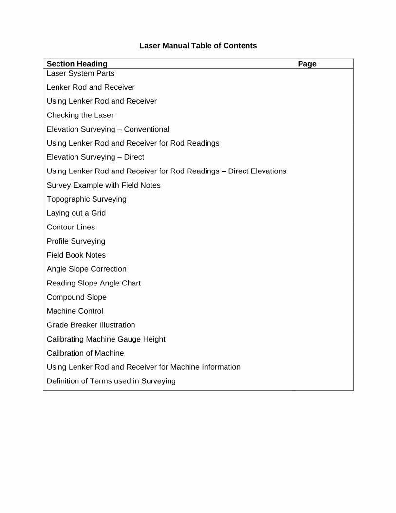
Laser Manual Table of Contents
Section Heading Page Laser System Parts
Lenker Rod and Receiver
Using Lenker Rod and Receiver
Checking the Laser
Elevation Surveying – Conventional
Using Lenker Rod and Receiver for Rod Readings
Elevation Surveying – Direct
Using Lenker Rod and Receiver for Rod Readings – Direct Elevations
Survey Example with Field Notes
Topographic Surveying
Laying out a Grid
Contour Lines
Profile Surveying
Field Book Notes
Angle Slope Correction
Reading Slope Angle Chart
Compound Slope
Machine Control
Grade Breaker Illustration
Calibrating Machine Gauge Height
Calibration of Machine
Using Lenker Rod and Receiver for Machine Information
Definition of Terms used in Surveying
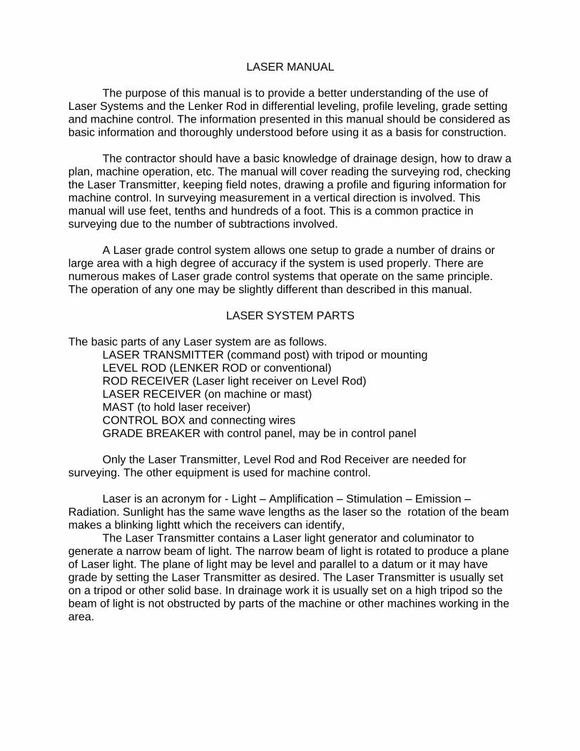
LASER MANUAL
The purpose of this manual is to provide a better understanding of the use of
Laser Systems and the Lenker Rod in differential leveling, profile leveling, grade setting and machine control. The information presented in this manual should be considered as basic information and thoroughly understood before using it as a basis for construction.
The contractor should have a basic knowledge of drainage design, how to draw a plan, machine operation, etc. The manual will cover reading the surveying rod, checking the Laser Transmitter, keeping field notes, drawing a profile and figuring information for machine control. In surveying measurement in a vertical direction is involved. This manual will use feet, tenths and hundreds of a foot. This is a common practice in surveying due to the number of subtractions involved.
A Laser grade control system allows one setup to grade a number of drains or large area with a high degree of accuracy if the system is used properly. There are numerous makes of Laser grade control systems that operate on the same principle. The operation of any one may be slightly different than described in this manual.
LASER SYSTEM PARTS The basic parts of any Laser system are as follows.
LASER TRANSMITTER (command post) with tripod or mounting LEVEL ROD (LENKER ROD or conventional) ROD RECEIVER (Laser light receiver on Level Rod) LASER RECEIVER (on machine or mast) MAST (to hold laser receiver) CONTROL BOX and connecting wires GRADE BREAKER with control panel, may be in control panel
Only the Laser Transmitter, Level Rod and Rod Receiver are needed for
surveying. The other equipment is used for machine control.
Laser is an acronym for - Light – Amplification – Stimulation – Emission – Radiation. Sunlight has the same wave lengths as the laser so the rotation of the beam makes a blinking lightt which the receivers can identify,
The Laser Transmitter contains a Laser light generator and columinator to generate a narrow beam of light. The narrow beam of light is rotated to produce a plane of Laser light. The plane of light may be level and parallel to a datum or it may have grade by setting the Laser Transmitter as desired. The Laser Transmitter is usually set on a tripod or other solid base. In drainage work it is usually set on a high tripod so the beam of light is not obstructed by parts of the machine or other machines working in the area.
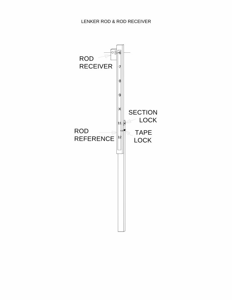
LENKER ROD & ROD RECEIVER
RODREFERENCE
TAPELOCK
ROD RECEIVER
9
12
X
11
7
8
6
SECTIONLOCK
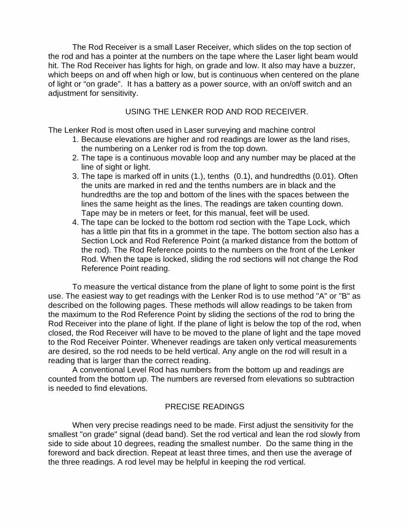
The Rod Receiver is a small Laser Receiver, which slides on the top section of
the rod and has a pointer at the numbers on the tape where the Laser light beam would hit. The Rod Receiver has lights for high, on grade and low. It also may have a buzzer, which beeps on and off when high or low, but is continuous when centered on the plane of light or “on grade”. It has a battery as a power source, with an on/off switch and an adjustment for sensitivity.
USING THE LENKER ROD AND ROD RECEIVER. The Lenker Rod is most often used in Laser surveying and machine control
1. Because elevations are higher and rod readings are lower as the land rises, the numbering on a Lenker rod is from the top down.
2. The tape is a continuous movable loop and any number may be placed at the line of sight or light.
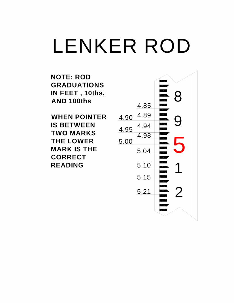
3. The tape is marked off in units (1.), tenths (0.1), and hundredths (0.01). Often the units are marked in red and the tenths numbers are in black and the hundredths are the top and bottom of the lines with the spaces between the lines the same height as the lines. The readings are taken counting down. Tape may be in meters or feet, for this manual, feet will be used.
4. The tape can be locked to the bottom rod section with the Tape Lock, which has a little pin that fits in a grommet in the tape. The bottom section also has a Section Lock and Rod Reference Point (a marked distance from the bottom of the rod). The Rod Reference points to the numbers on the front of the Lenker Rod. When the tape is locked, sliding the rod sections will not change the Rod Reference Point reading.
To measure the vertical distance from the plane of light to some point is the first
use. The easiest way to get readings with the Lenker Rod is to use method "A" or "B" as described on the following pages. These methods will allow readings to be taken from the maximum to the Rod Reference Point by sliding the sections of the rod to bring the Rod Receiver into the plane of light. If the plane of light is below the top of the rod, when closed, the Rod Receiver will have to be moved to the plane of light and the tape moved to the Rod Receiver Pointer. Whenever readings are taken only vertical measurements are desired, so the rod needs to be held vertical. Any angle on the rod will result in a reading that is larger than the correct reading.
A conventional Level Rod has numbers from the bottom up and readings are counted from the bottom up. The numbers are reversed from elevations so subtraction is needed to find elevations.
PRECISE READINGS
When very precise readings need to be made. First adjust the sensitivity for the smallest "on grade" signal (dead band). Set the rod vertical and lean the rod slowly from side to side about 10 degrees, reading the smallest number. Do the same thing in the foreword and back direction. Repeat at least three times, and then use the average of the three readings. A rod level may be helpful in keeping the rod vertical.
4.984.944.894.85
5.00
4.95
4.90
89
12
5
LENKER RODNOTE: ROD GRADUATIONS IN FEET , 10ths, AND 100ths
WHEN POINTER IS BETWEEN TWO MARKS THE LOWER MARK IS THE CORRECT READING
5.04
5.21
5.15
5.10
CHECKING THE LASER
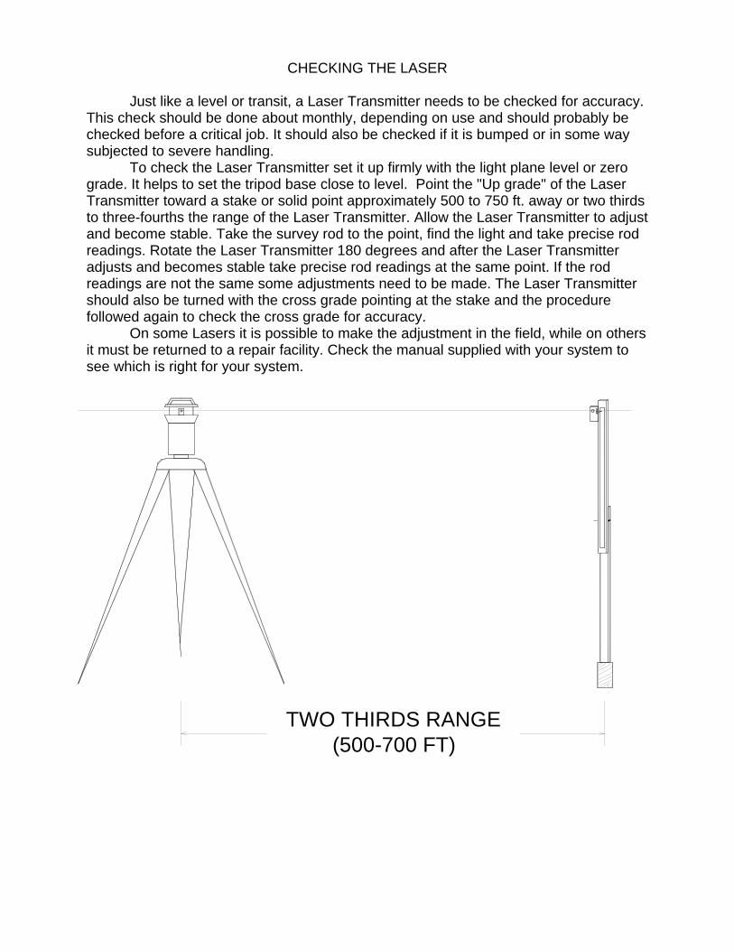
Just like a level or transit, a Laser Transmitter needs to be checked for accuracy. This check should be done about monthly, depending on use and should probably be checked before a critical job. It should also be checked if it is bumped or in some way subjected to severe handling.
To check the Laser Transmitter set it up firmly with the light plane level or zero grade. It helps to set the tripod base close to level. Point the "Up grade" of the Laser Transmitter toward a stake or solid point approximately 500 to 750 ft. away or two thirds to three-fourths the range of the Laser Transmitter. Allow the Laser Transmitter to adjust and become stable. Take the survey rod to the point, find the light and take precise rod readings. Rotate the Laser Transmitter 180 degrees and after the Laser Transmitter adjusts and becomes stable take precise rod readings at the same point. If the rod readings are not the same some adjustments need to be made. The Laser Transmitter should also be turned with the cross grade pointing at the stake and the procedure followed again to check the cross grade for accuracy.
On some Lasers it is possible to make the adjustment in the field, while on others it must be returned to a repair facility. Check the manual supplied with your system to see which is right for your system.
TWO THIRDS RANGE (500-700 FT)
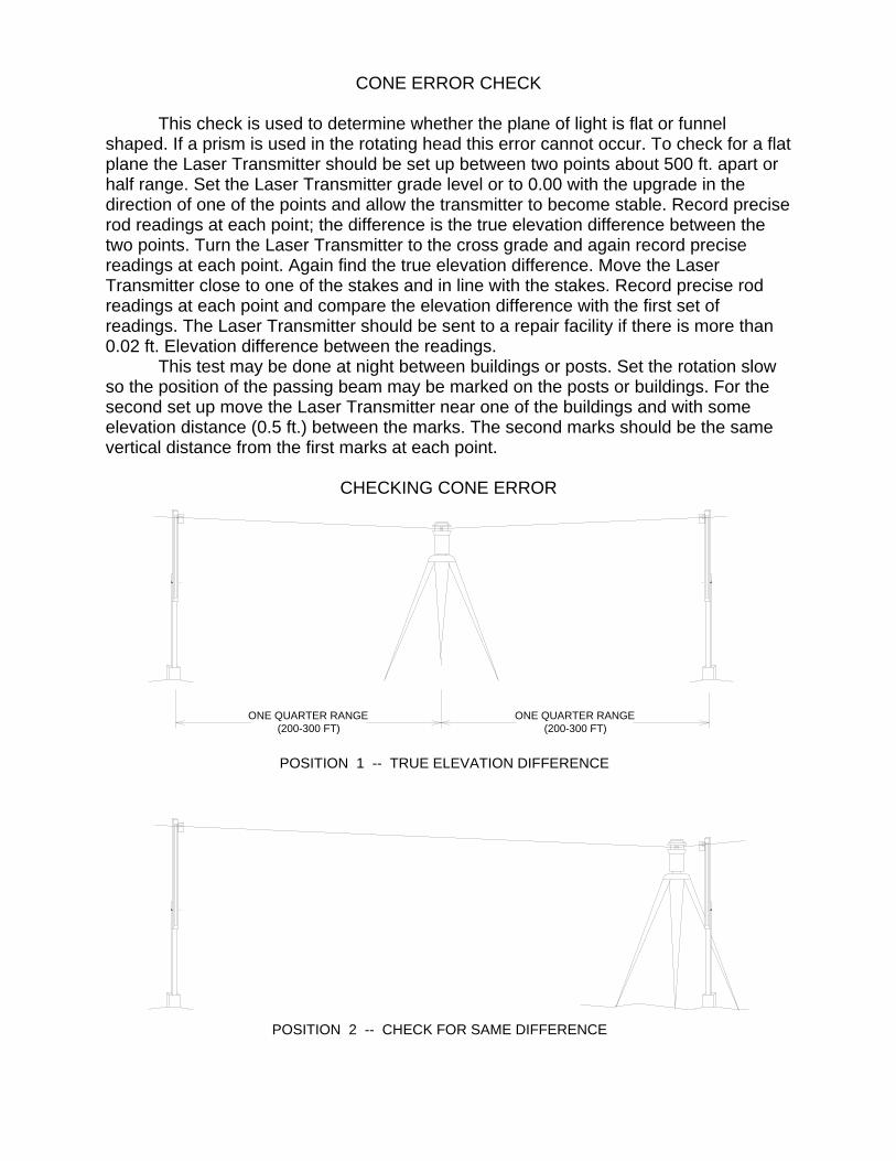
CONE ERROR CHECK
This check is used to determine whether the plane of light is flat or funnel shaped. If a prism is used in the rotating head this error cannot occur. To check for a flat plane the Laser Transmitter should be set up between two points about 500 ft. apart or half range. Set the Laser Transmitter grade level or to 0.00 with the upgrade in the direction of one of the points and allow the transmitter to become stable. Record precise rod readings at each point; the difference is the true elevation difference between the two points. Turn the Laser Transmitter to the cross grade and again record precise readings at each point. Again find the true elevation difference. Move the Laser Transmitter close to one of the stakes and in line with the stakes. Record precise rod readings at each point and compare the elevation difference with the first set of readings. The Laser Transmitter should be sent to a repair facility if there is more than 0.02 ft. Elevation difference between the readings.
This test may be done at night between buildings or posts. Set the rotation slow so the position of the passing beam may be marked on the posts or buildings. For the second set up move the Laser Transmitter near one of the buildings and with some elevation distance (0.5 ft.) between the marks. The second marks should be the same vertical distance from the first marks at each point.
CHECKING CONE ERROR
POSITION 2 -- CHECK FOR SAME DIFFERENCE
POSITION 1 -- TRUE ELEVATION DIFFERENCE
ONE QUARTER RANGE (200-300 FT)
ONE QUARTER RANGE (200-300 FT)
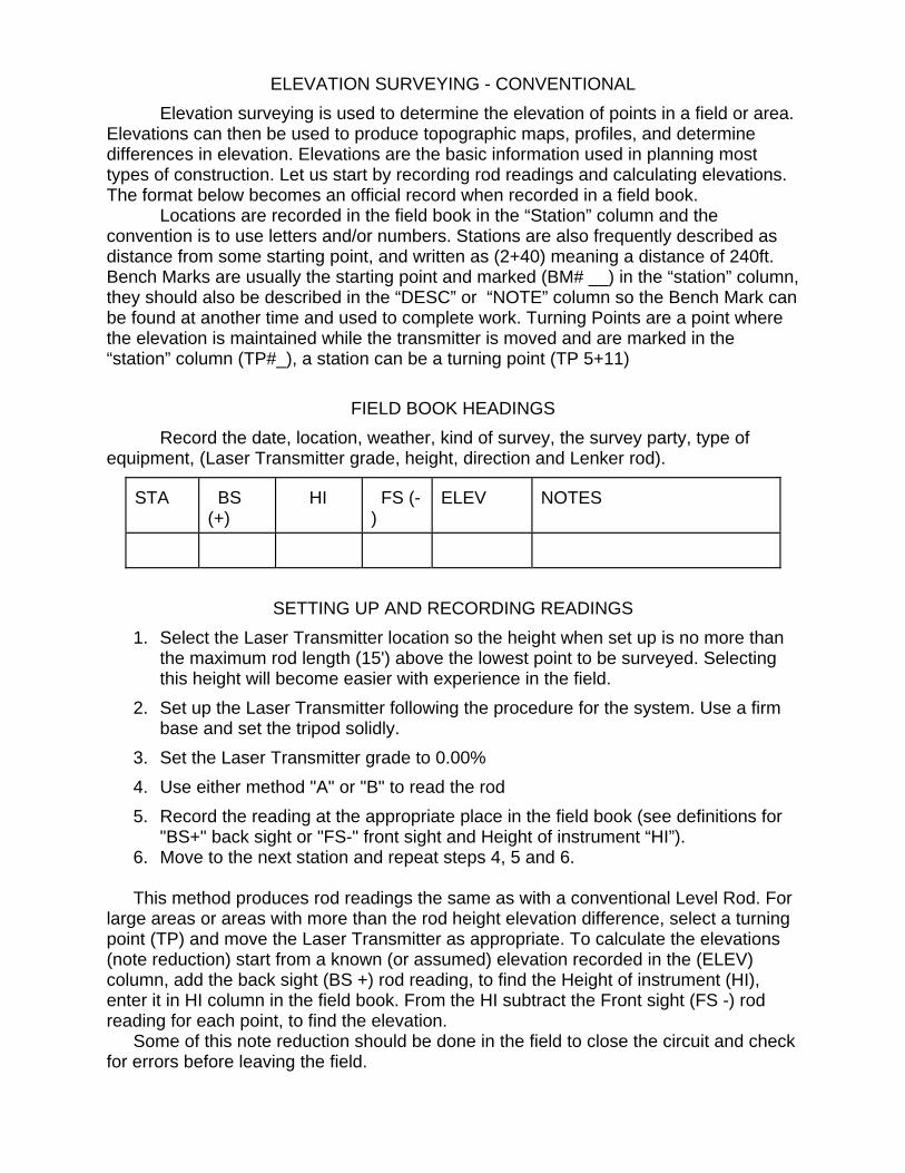
ELEVATION SURVEYING - CONVENTIONAL Elevation surveying is used to determine the elevation of points in a field or area.
Elevations can then be used to produce topographic maps, profiles, and determine differences in elevation. Elevations are the basic information used in planning most types of construction. Let us start by recording rod readings and calculating elevations. The format below becomes an official record when recorded in a field book.
Locations are recorded in the field book in the “Station” column and the convention is to use letters and/or numbers. Stations are also frequently described as distance from some starting point, and written as (2+40) meaning a distance of 240ft. Bench Marks are usually the starting point and marked (BM# __) in the “station” column, they should also be described in the “DESC” or “NOTE” column so the Bench Mark can be found at another time and used to complete work. Turning Points are a point where the elevation is maintained while the transmitter is moved and are marked in the “station” column (TP#_), a station can be a turning point (TP 5+11)
FIELD BOOK HEADINGS Record the date, location, weather, kind of survey, the survey party, type of
equipment, (Laser Transmitter grade, height, direction and Lenker rod). STA
BS (+)
HI
FS (-)
ELEV
NOTES
SETTING UP AND RECORDING READINGS
1. Select the Laser Transmitter location so the height when set up is no more than the maximum rod length (15') above the lowest point to be surveyed. Selecting this height will become easier with experience in the field.
2. Set up the Laser Transmitter following the procedure for the system. Use a firm base and set the tripod solidly.
3. Set the Laser Transmitter grade to 0.00% 4. Use either method "A" or "B" to read the rod 5. Record the reading at the appropriate place in the field book (see definitions for
"BS+" back sight or "FS-" front sight and Height of instrument “HI”). 6. Move to the next station and repeat steps 4, 5 and 6.
This method produces rod readings the same as with a conventional Level Rod. For
large areas or areas with more than the rod height elevation difference, select a turning point (TP) and move the Laser Transmitter as appropriate. To calculate the elevations (note reduction) start from a known (or assumed) elevation recorded in the (ELEV) column, add the back sight (BS +) rod reading, to find the Height of instrument (HI), enter it in HI column in the field book. From the HI subtract the Front sight (FS -) rod reading for each point, to find the elevation. Some of this note reduction should be done in the field to close the circuit and check for errors before leaving the field.
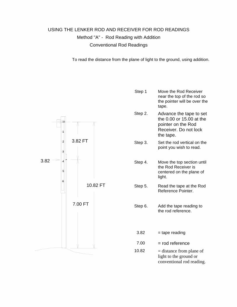
USING THE LENKER ROD AND RECEIVER FOR ROD READINGS
Method "A" - Rod Reading with Addition Conventional Rod Readings
Step 1 Move the Rod Receiver near the top of the rod so the pointer will be over the tape.
Step 2. Advance the tape to set the 0.00 or 15.00 at the pointer on the Rod Receiver. Do not lock the tape.
Step 3. Set the rod vertical on the point you wish to read.
Step 4. Move the top section until the Rod Receiver is centered on the plane of light.
Step 5. Read the tape at the Rod Reference Pointer.
Step 6. Add the tape reading to the rod reference.
3.82 = tape reading
7.00 = rod reference 10.82 = distance from plane of
light to the ground or conventional rod reading.
To read the distance from the plane of light to the ground, using addition.
7.00 FT
3.82 FT
6
3.82
5
4
3
15
2
1
10.82 FT
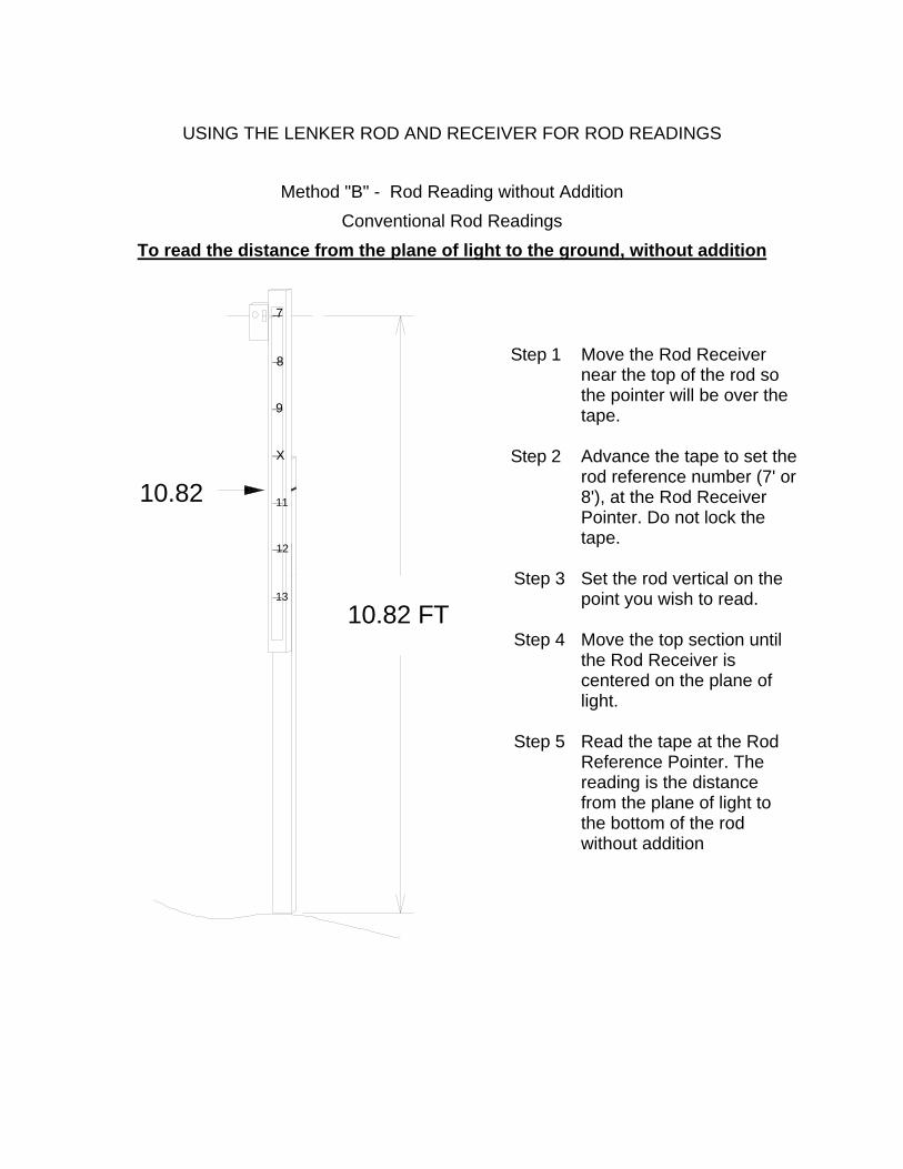
USING THE LENKER ROD AND RECEIVER FOR ROD READINGS
Method "B" - Rod Reading without Addition Conventional Rod Readings
To read the distance from the plane of light to the ground, without addition
10.82 FT
10.82
12
13
11
X
9
8
7
Step 1 Move the Rod Receiver near the top of the rod so the pointer will be over the tape.
Step 2 Advance the tape to set the rod reference number (7' or 8'), at the Rod Receiver Pointer. Do not lock the tape.
Step 3 Set the rod vertical on the point you wish to read.
Step 4 Move the top section until the Rod Receiver is centered on the plane of light.
Step 5 Read the tape at the Rod Reference Pointer. The reading is the distance from the plane of light to the bottom of the rod without addition
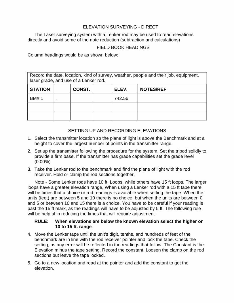
ELEVATION SURVEYING - DIRECT
The Laser surveying system with a Lenker rod may be used to read elevations directly and avoid some of the note reduction (subtraction and calculations)
FIELD BOOK HEADINGS Column headings would be as shown below:
SETTING UP AND RECORDING ELEVATIONS
1. Select the transmitter location so the plane of light is above the Benchmark and at a height to cover the largest number of points in the transmitter range.
2. Set up the transmitter following the procedure for the system. Set the tripod solidly to provide a firm base. If the transmitter has grade capabilities set the grade level (0.00%)
3. Take the Lenker rod to the benchmark and find the plane of light with the rod receiver. Hold or clamp the rod sections together. Note - Some Lenker rods have 10 ft. Loops, while others have 15 ft loops. The larger
loops have a greater elevation range, When using a Lenker rod with a 15 ft tape there will be times that a choice or rod readings is available when setting the tape. When the units (feet) are between 5 and 10 there is no choice, but when the units are between 0 and 5 or between 10 and 15 there is a choice. You have to be careful if your reading is past the 15 ft mark, as the readings will have to be adjusted by 5 ft. The following rule will be helpful in reducing the times that will require adjustment.
RULE: When elevations are below the known elevation select the higher or 10 to 15 ft. range.
4. Move the Lenker tape until the unit’s digit, tenths, and hundreds of feet of the benchmark are in line with the rod receiver pointer and lock the tape. Check the setting, as any error will be reflected in the readings that follow. The Constant is the Elevation minus the tape setting. Record the constant. Loosen the clamp on the rod sections but leave the tape locked.
5. Go to a new location and read at the pointer and add the constant to get the elevation.
Record the date, location, kind of survey, weather, people and their job, equipment, laser grade, and use of a Lenker rod. STATION
CONST.
ELEV.
NOTES/REF
BM# 1
.
742.56
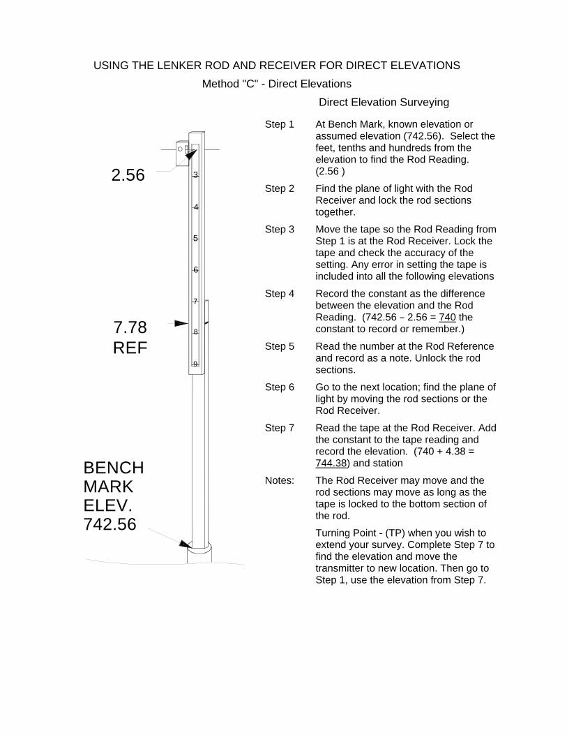
USING THE LENKER ROD AND RECEIVER FOR DIRECT ELEVATIONS
Method "C" - Direct Elevations Direct Elevation Surveying
7.78REF
2.56
BENCHMARKELEV.742.56
8
9
7
6
5
4
3
Step 1 At Bench Mark, known elevation or assumed elevation (742.56). Select the feet, tenths and hundreds from the elevation to find the Rod Reading. (2.56 )
Step 2 Find the plane of light with the Rod Receiver and lock the rod sections together.
Step 3 Move the tape so the Rod Reading from Step 1 is at the Rod Receiver. Lock the tape and check the accuracy of the setting. Any error in setting the tape is included into all the following elevations
Step 4 Record the constant as the difference between the elevation and the Rod Reading. (742.56 B 2.56 = 740 the constant to record or remember.)
Step 5 Read the number at the Rod Reference and record as a note. Unlock the rod sections.
Step 6 Go to the next location; find the plane of light by moving the rod sections or the Rod Receiver.
Step 7 Read the tape at the Rod Receiver. Add the constant to the tape reading and record the elevation. (740 + 4.38 = 744.38) and station
Notes: The Rod Receiver may move and the rod sections may move as long as the tape is locked to the bottom section of the rod.
Turning Point - (TP) when you wish to extend your survey. Complete Step 7 to find the elevation and move the transmitter to new location. Then go to Step 1, use the elevation from Step 7.
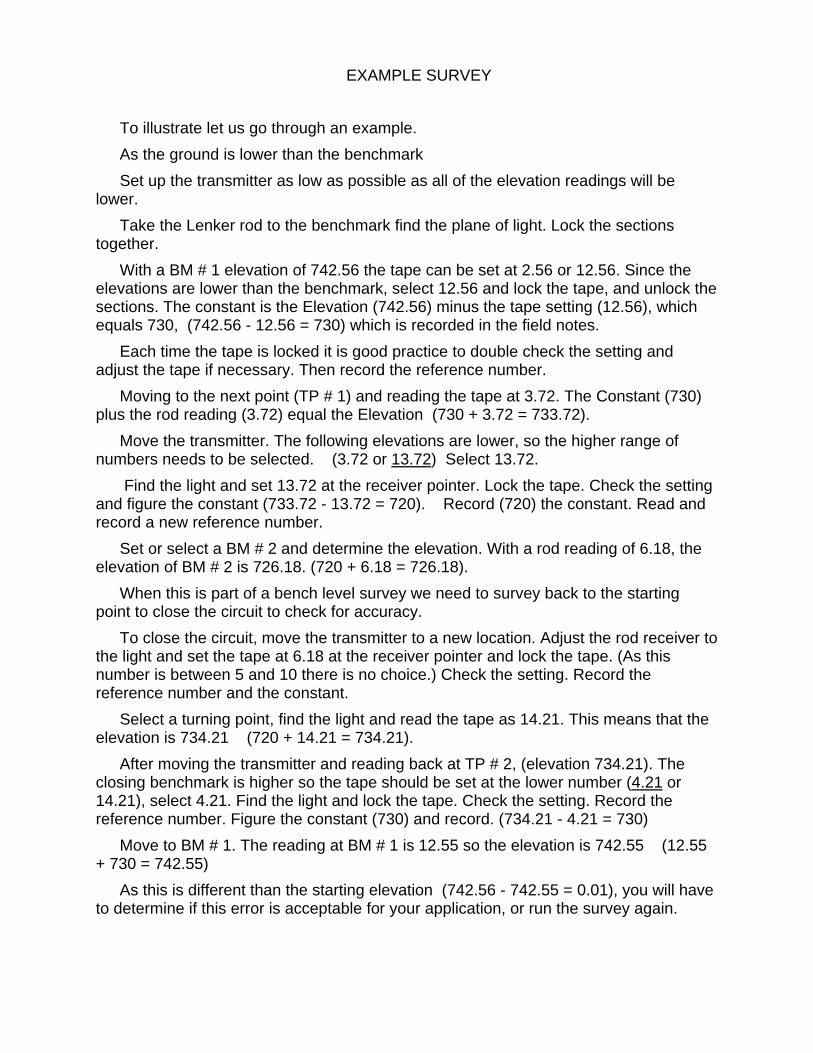
EXAMPLE SURVEY
To illustrate let us go through an example. As the ground is lower than the benchmark Set up the transmitter as low as possible as all of the elevation readings will be lower. Take the Lenker rod to the benchmark find the plane of light. Lock the sections together. With a BM # 1 elevation of 742.56 the tape can be set at 2.56 or 12.56. Since the elevations are lower than the benchmark, select 12.56 and lock the tape, and unlock the sections. The constant is the Elevation (742.56) minus the tape setting (12.56), which equals 730, (742.56 - 12.56 = 730) which is recorded in the field notes.
Each time the tape is locked it is good practice to double check the setting and adjust the tape if necessary. Then record the reference number.
Moving to the next point (TP # 1) and reading the tape at 3.72. The Constant (730) plus the rod reading (3.72) equal the Elevation (730 + 3.72 = 733.72).
Move the transmitter. The following elevations are lower, so the higher range of numbers needs to be selected. (3.72 or 13.72) Select 13.72.
Find the light and set 13.72 at the receiver pointer. Lock the tape. Check the setting and figure the constant (733.72 - 13.72 = 720). Record (720) the constant. Read and record a new reference number.
Set or select a BM # 2 and determine the elevation. With a rod reading of 6.18, the elevation of BM # 2 is 726.18. (720 + 6.18 = 726.18).
When this is part of a bench level survey we need to survey back to the starting point to close the circuit to check for accuracy.
To close the circuit, move the transmitter to a new location. Adjust the rod receiver to the light and set the tape at 6.18 at the receiver pointer and lock the tape. (As this number is between 5 and 10 there is no choice.) Check the setting. Record the reference number and the constant.
Select a turning point, find the light and read the tape as 14.21. This means that the elevation is 734.21 (720 + 14.21 = 734.21).
After moving the transmitter and reading back at TP # 2, (elevation 734.21). The closing benchmark is higher so the tape should be set at the lower number (4.21 or 14.21), select 4.21. Find the light and lock the tape. Check the setting. Record the reference number. Figure the constant (730) and record. (734.21 - 4.21 = 730)
Move to BM # 1. The reading at BM # 1 is 12.55 so the elevation is 742.55 (12.55 + 730 = 742.55)
As this is different than the starting elevation (742.56 - 742.55 = 0.01), you will have to determine if this error is acceptable for your application, or run the survey again.
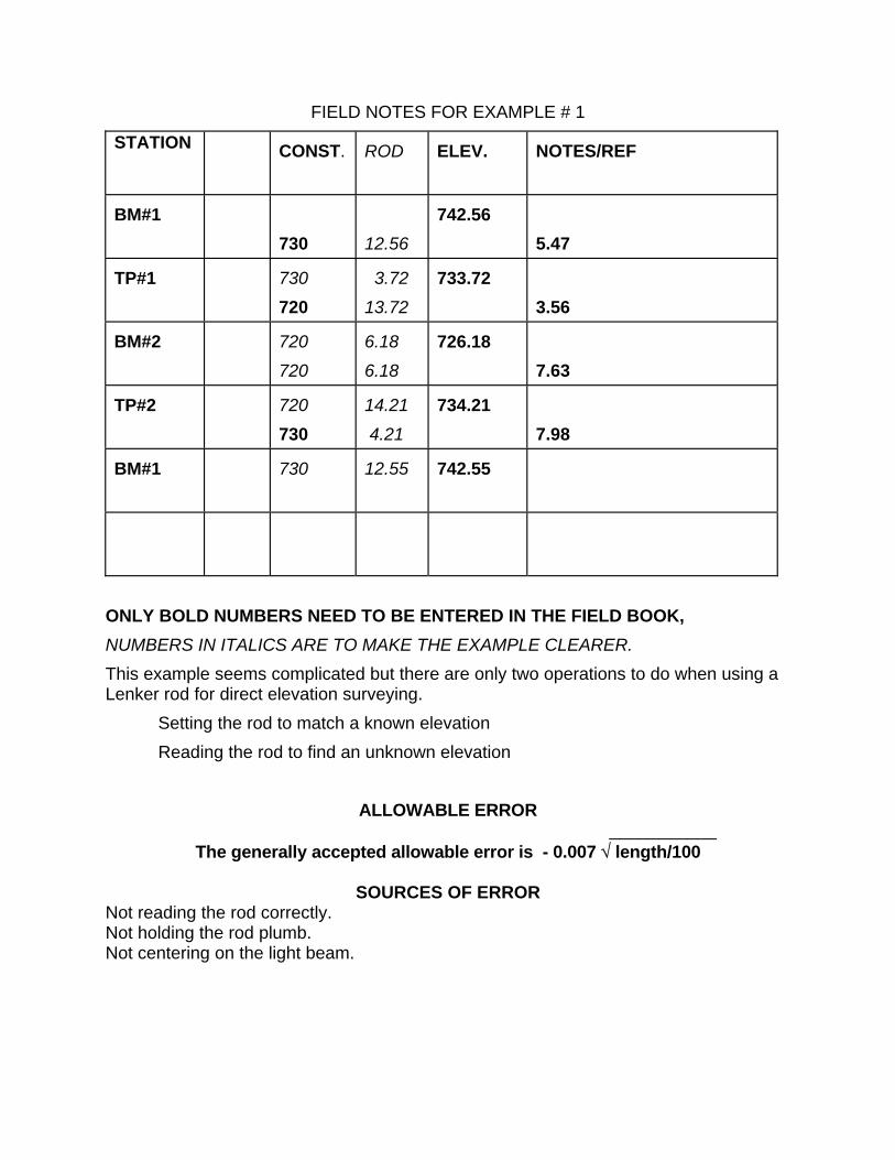
FIELD NOTES FOR EXAMPLE # 1
STATION CONST.
ROD
ELEV.
NOTES/REF
BM#1
730
12.56
742.56
5.47
TP#1
730 720
3.72
13.72
733.72
3.56
BM#2
720
720
6.18
6.18
726.18
7.63
TP#2
720 730
14.21
4.21
734.21
7.98
BM#1
730
12.55
742.55
ONLY BOLD NUMBERS NEED TO BE ENTERED IN THE FIELD BOOK, NUMBERS IN ITALICS ARE TO MAKE THE EXAMPLE CLEARER. This example seems complicated but there are only two operations to do when using a Lenker rod for direct elevation surveying. Setting the rod to match a known elevation Reading the rod to find an unknown elevation
ALLOWABLE ERROR ___________
The generally accepted allowable error is - 0.007 √ length/100
SOURCES OF ERROR Not reading the rod correctly. Not holding the rod plumb. Not centering on the light beam.
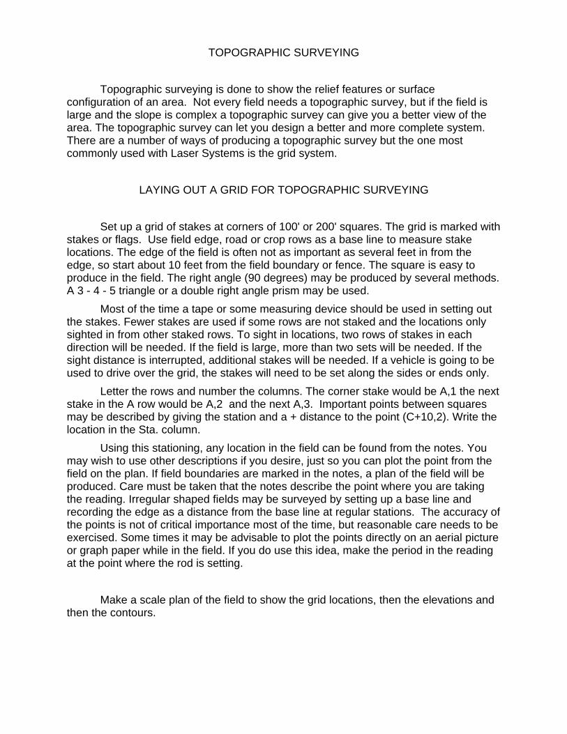
TOPOGRAPHIC SURVEYING
Topographic surveying is done to show the relief features or surface configuration of an area. Not every field needs a topographic survey, but if the field is large and the slope is complex a topographic survey can give you a better view of the area. The topographic survey can let you design a better and more complete system. There are a number of ways of producing a topographic survey but the one most commonly used with Laser Systems is the grid system.
LAYING OUT A GRID FOR TOPOGRAPHIC SURVEYING
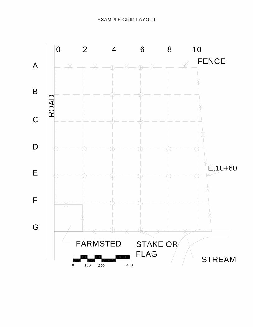
Set up a grid of stakes at corners of 100' or 200' squares. The grid is marked with stakes or flags. Use field edge, road or crop rows as a base line to measure stake locations. The edge of the field is often not as important as several feet in from the edge, so start about 10 feet from the field boundary or fence. The square is easy to produce in the field. The right angle (90 degrees) may be produced by several methods. A 3 - 4 - 5 triangle or a double right angle prism may be used.
Most of the time a tape or some measuring device should be used in setting out the stakes. Fewer stakes are used if some rows are not staked and the locations only sighted in from other staked rows. To sight in locations, two rows of stakes in each direction will be needed. If the field is large, more than two sets will be needed. If the sight distance is interrupted, additional stakes will be needed. If a vehicle is going to be used to drive over the grid, the stakes will need to be set along the sides or ends only.
Letter the rows and number the columns. The corner stake would be A,1 the next stake in the A row would be A,2 and the next A,3. Important points between squares may be described by giving the station and a + distance to the point (C+10,2). Write the location in the Sta. column.
Using this stationing, any location in the field can be found from the notes. You may wish to use other descriptions if you desire, just so you can plot the point from the field on the plan. If field boundaries are marked in the notes, a plan of the field will be produced. Care must be taken that the notes describe the point where you are taking the reading. Irregular shaped fields may be surveyed by setting up a base line and recording the edge as a distance from the base line at regular stations. The accuracy of the points is not of critical importance most of the time, but reasonable care needs to be exercised. Some times it may be advisable to plot the points directly on an aerial picture or graph paper while in the field. If you do use this idea, make the period in the reading at the point where the rod is setting.
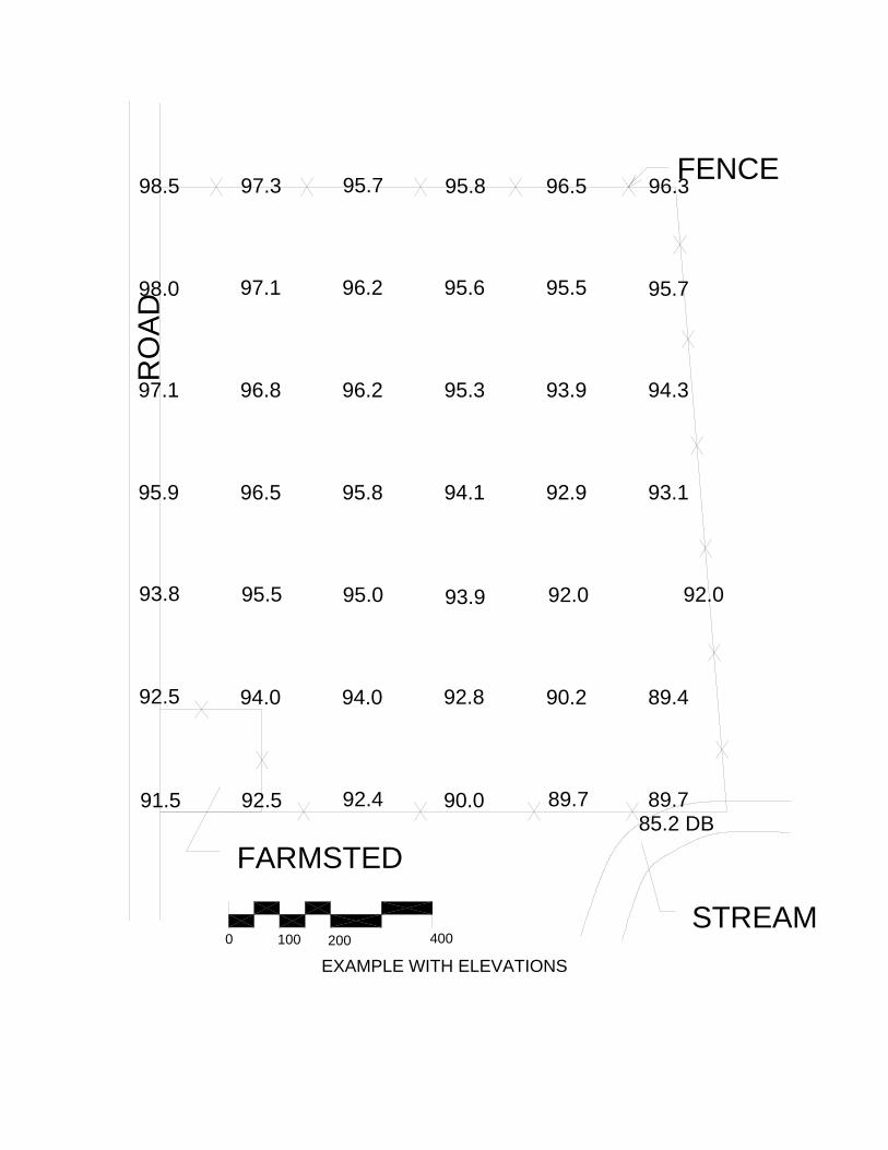
Make a scale plan of the field to show the grid locations, then the elevations and
then the contours.
EXAMPLE GRID LAYOUT
STAKE ORFLAG
0 2 4
E,10+60
STREAM
RO
AD
D
C
A
B
E
FARMSTED
0
G
F
200100 400
106 8FENCE
EXAMPLE WITH ELEVATIONS
98.0
95.8
96.2
96.5
96.8
96.2
97.3
97.1
95.7
92.0 92.0
STREAM
89.785.2 DB
89.494.0
92.4
RO
AD
95.9
97.1
98.5
93.9
90.0
92.8
94.1
95.3
95.8
95.6
93.8 95.5 95.0
FARMSTED
0
91.5
92.5
200100 400
94.0
92.5 89.7
90.2
96.3
94.3
93.1
95.7
93.9
92.9
95.5
96.5FENCE
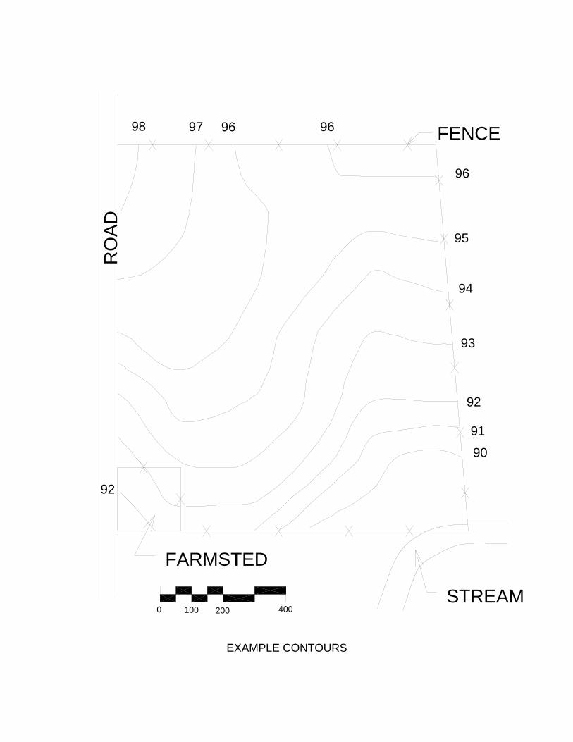
CONTOUR LINES
A Contour line is a line connecting points on the same elevation. There are some rules that will be helpful in drawing and working with contour lines. 1. Contour lines never cross (except in an overhanging cliff). 2. Contours are always one continuous line without an end. (This may not
happen on an individual map).
To convert the grid map with elevations marked upon it there are some assumptions which will help in understanding and drawing contours. Assume the slope of the land is constant between the readings. If this is not true additional points should be recorded until it is nearly true. The contour interval must be selected, (1 foot, 2 foot, 5 foot, 20 foot, etc.). The closer the contour interval the more lines on the map and the more detail shown, also the more work to produce the map. The use and the slope of the land will determine the interval. Level ground will have fewer contours than hilly land. For subsurface drainage work 1-foot contours are about right. Do not change contour intervals without marking it well as the appearance of the slope will be misleading. There are many ways and programs to draw contours, but the following is an easy way to teach drawing contours that is straight foreword. Start at any point to draw a contour. Between two points determine the elevation difference and the number of contours between those elevations. Using points 93.8 and 95.9 there are two 1-foot contours (94 and 95) between them. To find the location of the contours between the points, the distance is divided into (95.9 - 93.8 = 2.1) 2.1 tenths of a foot or 21 spaces. The first contour above the 93.8 point is 94, this is (94 - 93.8 = 2) 2/21 or 0.095% of the distance. Place a dot at the point. The second contour line is 95, this is 12/21 or 0.57% up from the 93.8 point. Place a dot at the point. It could also be determined down from the 95.9 point as (95.9 - 95 = .9) 9/21 or 0.428% down from 95.9 toward 93.8. The 94 contour would be (95.9 - 94 = 1.9) 19/21 or 0.904% down from 95.9. Select another set of points and do the same procedure until several points are plotted, then connect the dots of the same elevation in a smooth line. The contour line may be straight if the slope of the land is even, however it is most often curved. It is helpful to extend the line outside of the map a short distance and label it with the contour elevation. On some maps heavier lines are labeled and the others left unlabeled which can reduce clutter. When a knob or depression is shown by a closed loop, it will be difficult to determine which is shown. An elevation point inside the loop will be helpful or the depression may have short lines in the direction of the low area.
EXAMPLE CONTOURS
98 9697
92
STREAM
RO
AD
FARMSTED
0
92
200100 400
91
90
96
93
95
94
FENCE
96
PROFILE SURVEYING
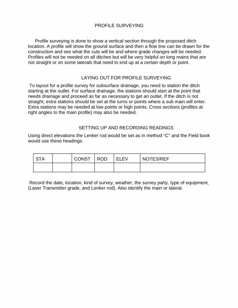
Profile surveying is done to show a vertical section through the proposed ditch location. A profile will show the ground surface and then a flow line can be drawn for the construction and see what the cuts will be and where grade changes will be needed. Profiles will not be needed on all ditches but will be very helpful on long mains that are not straight or on some laterals that need to end up at a certain depth or point.
LAYING OUT FOR PROFILE SURVEYING To layout for a profile survey for subsurface drainage, you need to station the ditch starting at the outlet. For surface drainage, the stations should start at the point that needs drainage and proceed as far as necessary to get an outlet. If the ditch is not straight, extra stations should be set at the turns or points where a sub main will enter. Extra stations may be needed at low points or high points. Cross sections (profiles at right angles to the main profile) may also be needed.
SETTING UP AND RECORDING READINGS Using direct elevations the Lenker rod would be set as in method AC@ and the Field book would use these headings.
STA
CONST
ROD
ELEV
NOTES/REF
Record the date, location, kind of survey, weather, the survey party, type of equipment, (Laser Transmitter grade, and Lenker rod). Also identify the main or lateral.
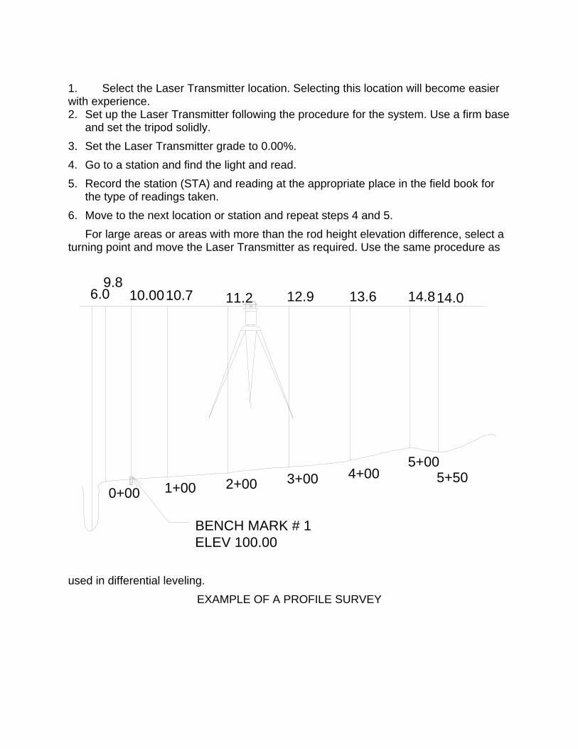
1. Select the Laser Transmitter location. Selecting this location will become easier with experience. 2. Set up the Laser Transmitter following the procedure for the system. Use a firm base
and set the tripod solidly. 3. Set the Laser Transmitter grade to 0.00%. 4. Go to a station and find the light and read. 5. Record the station (STA) and reading at the appropriate place in the field book for
the type of readings taken. 6. Move to the next location or station and repeat steps 4 and 5.
For large areas or areas with more than the rod height elevation difference, select a turning point and move the Laser Transmitter as required. Use the same procedure as
used in differential leveling. EXAMPLE OF A PROFILE SURVEY
3+00
12.9
BENCH MARK # 1ELEV 100.00
1+000+00 2+00
10.79.8
6.0 10.00 11.2
5+004+00 5+50
13.6 14.014.8
FIELD BOOK NOTES
STA
CONST
ROD
ELEV
NOTES/REF
BM#1
90
10.00
100.0
BM# 1 TOP OF HUB
0+00
6.0
96.0
DITCH BOTTOM
0+05
9.8
99.8
1+00
10.7
100.7
2+00
11.2
101.2
3+00
12.9
102.9
4+00
13.6
103.6
5+00
14.8
104.8
5+50
14.0
104.0
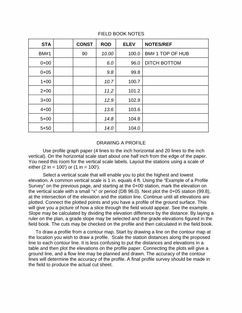
DRAWING A PROFILE
Use profile graph paper (4 lines to the inch horizontal and 20 lines to the inch vertical). On the horizontal scale start about one half inch from the edge of the paper. You need this room for the vertical scale labels. Layout the stations using a scale of either (2 in = 100') or (1 in = 100').
Select a vertical scale that will enable you to plot the highest and lowest elevation. A common vertical scale is 1 in. equals 4 ft. Using the “Example of a Profile Survey” on the previous page, and starting at the 0+00 station, mark the elevation on the vertical scale with a small Ax@ or period (DB 96.0). Next plot the 0+05 station (99.8), at the intersection of the elevation and the station line. Continue until all elevations are plotted. Connect the plotted points and you have a profile of the ground surface. This will give you a picture of how a slice through the field would appear. See the example. Slope may be calculated by dividing the elevation difference by the distance. By laying a ruler on the plan, a grade slope may be selected and the grade elevations figured in the field book. The cuts may be checked on the profile and then calculated in the field book.
To draw a profile from a contour map. Start by drawing a line on the contour map at the location you wish to draw a profile. Scale the station distances along the proposed line to each contour line. It is less confusing to put the distances and elevations in a table and then plot the elevations on the profile paper. Connecting the plots will give a ground line, and a flow line may be planned and drawn. The accuracy of the contour lines will determine the accuracy of the profile. A final profile survey should be made in the field to produce the actual cut sheet.
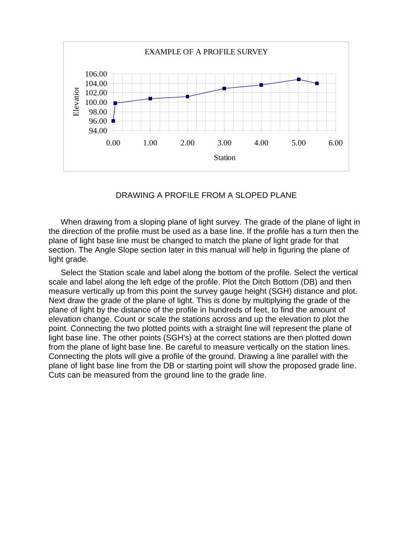
EXAMPLE OF A PROFILE SURVEY
94.0096.0098.00
100.00102.00104.00106.00
0.00 1.00 2.00 3.00 4.00 5.00 6.00
Station
Elev
atio
n
DRAWING A PROFILE FROM A SLOPED PLANE
When drawing from a sloping plane of light survey. The grade of the plane of light in the direction of the profile must be used as a base line. If the profile has a turn then the plane of light base line must be changed to match the plane of light grade for that section. The Angle Slope section later in this manual will help in figuring the plane of light grade.
Select the Station scale and label along the bottom of the profile. Select the vertical scale and label along the left edge of the profile. Plot the Ditch Bottom (DB) and then measure vertically up from this point the survey gauge height (SGH) distance and plot. Next draw the grade of the plane of light. This is done by multiplying the grade of the plane of light by the distance of the profile in hundreds of feet, to find the amount of elevation change. Count or scale the stations across and up the elevation to plot the point. Connecting the two plotted points with a straight line will represent the plane of light base line. The other points (SGH's) at the correct stations are then plotted down from the plane of light base line. Be careful to measure vertically on the station lines. Connecting the plots will give a profile of the ground. Drawing a line parallel with the plane of light base line from the DB or starting point will show the proposed grade line. Cuts can be measured from the ground line to the grade line.
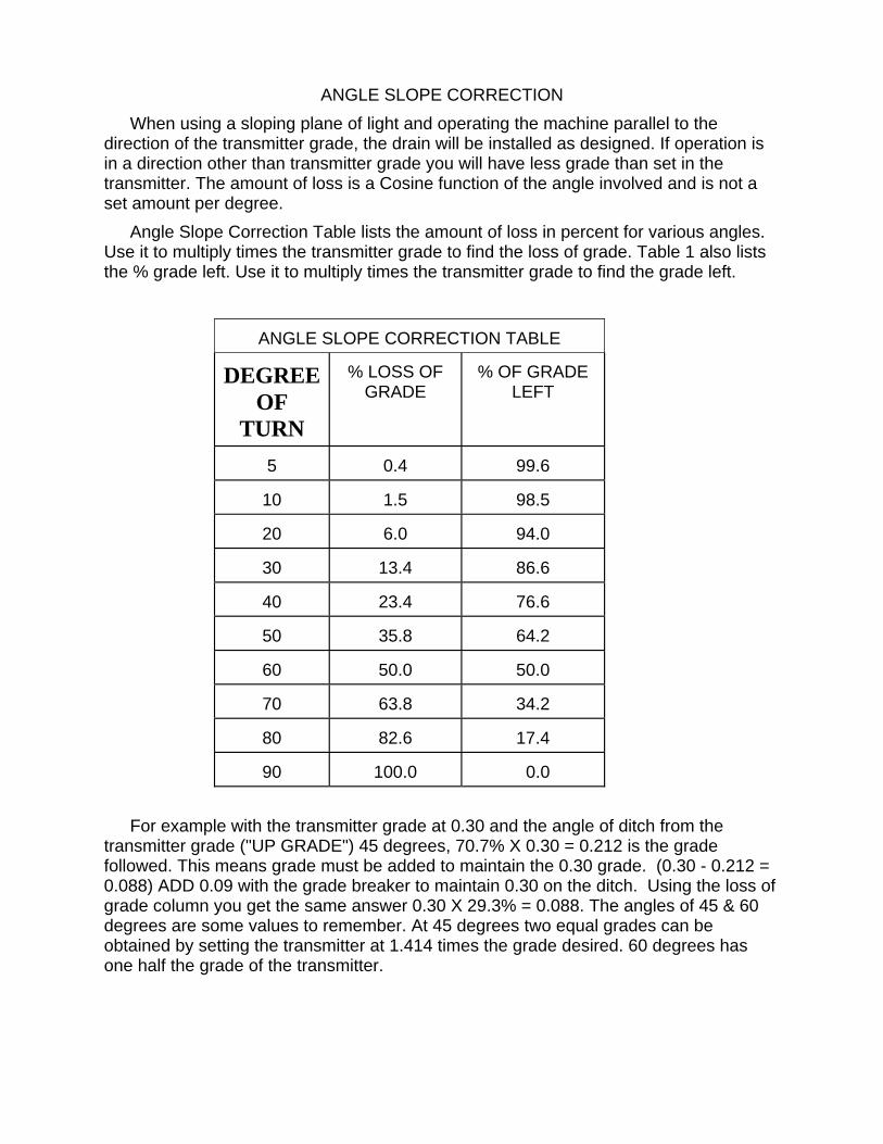
ANGLE SLOPE CORRECTION When using a sloping plane of light and operating the machine parallel to the
direction of the transmitter grade, the drain will be installed as designed. If operation is in a direction other than transmitter grade you will have less grade than set in the transmitter. The amount of loss is a Cosine function of the angle involved and is not a set amount per degree.
Angle Slope Correction Table lists the amount of loss in percent for various angles. Use it to multiply times the transmitter grade to find the loss of grade. Table 1 also lists the % grade left. Use it to multiply times the transmitter grade to find the grade left.
ANGLE SLOPE CORRECTION TABLE
DEGREE
OF TURN
% LOSS OF
GRADE
% OF GRADE
LEFT
5
0.4
99.6
10
1.5
98.5
20
6.0
94.0
30
13.4
86.6
40
23.4
76.6
50
35.8
64.2
60
50.0
50.0
70
63.8
34.2
80
82.6
17.4
90
100.0
0.0
For example with the transmitter grade at 0.30 and the angle of ditch from the
transmitter grade ("UP GRADE") 45 degrees, 70.7% X 0.30 = 0.212 is the grade followed. This means grade must be added to maintain the 0.30 grade. (0.30 - 0.212 = 0.088) ADD 0.09 with the grade breaker to maintain 0.30 on the ditch. Using the loss of grade column you get the same answer 0.30 X 29.3% = 0.088. The angles of 45 & 60 degrees are some values to remember. At 45 degrees two equal grades can be obtained by setting the transmitter at 1.414 times the grade desired. 60 degrees has one half the grade of the transmitter.
ANGLE SLOPE CHART
9008
7
7523
3
423 34
2 259
207
174
155
106
129
350
250
200
354
300
075
100
039
052
106
212
346
260
1514
519329
030 20
173
141
130
283 07
8
150
"0" G
RA
DE181
400
-129
-207
-181
-155
07510
6
078
052
039
100
193
17329
026
035
4 283
141
346
212
130
150
12925
030
040
0 350
155
181
207
200
104
-052
-078
-026
-104
105-2
59-1
74 -342
9008
725942
334
2
7517
4
-087
233
-233"0
" GR
AD
E
AN
GLE
- S
LOP
E C
HA
RT
145
6063
669
3
566
495
779866
30 819
707
766
676
5060
48358077
3
940
966 869
8090 70
906
606
520
985
15
996
45 574
643
483
580
676
520
693 60
6
773
940
869
966
495
566
643
63681930
866
707
766
906 779
15
985
996
6057
445
100
UP
GR
AD
E
45050
042
438
643
340
386
433
424
500
450
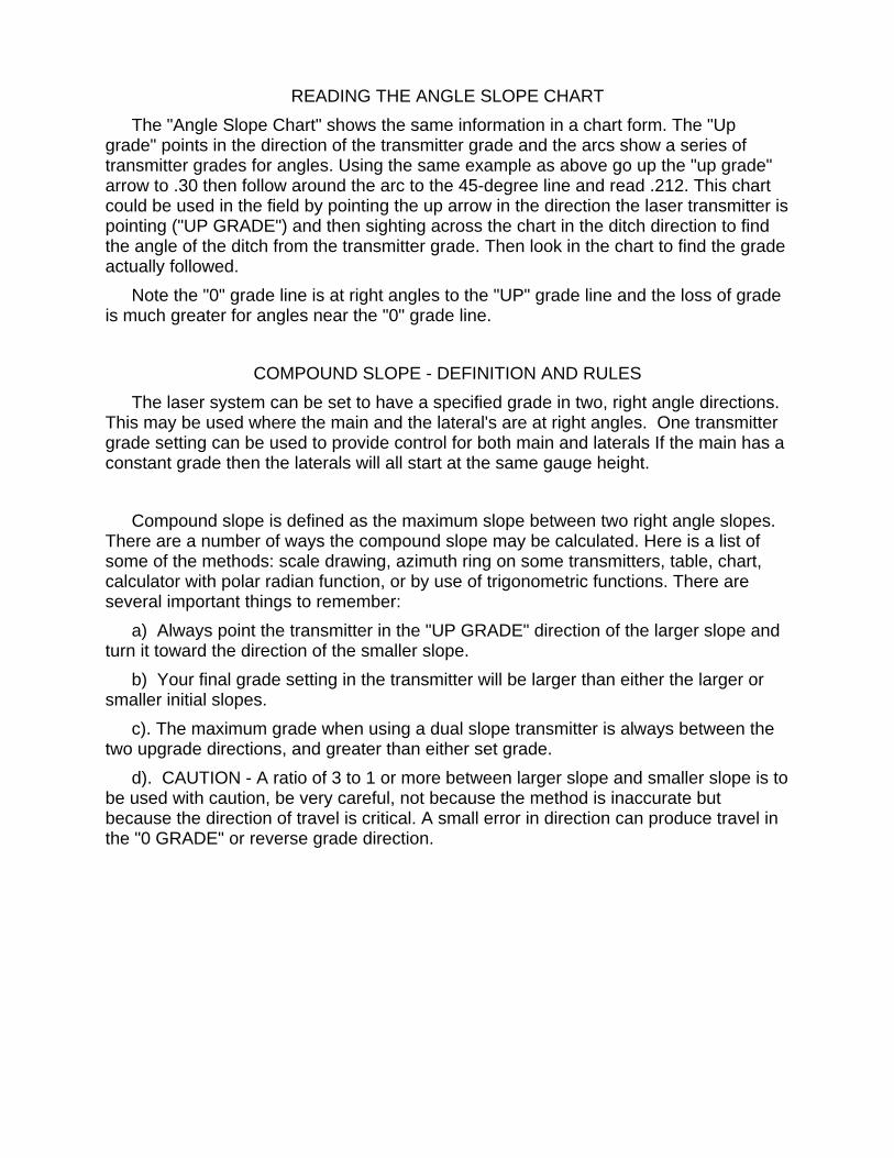
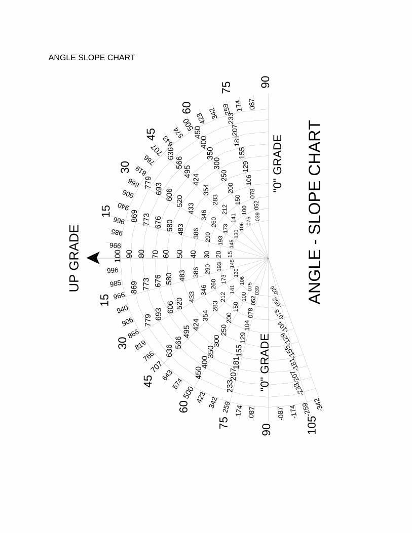
READING THE ANGLE SLOPE CHART The "Angle Slope Chart" shows the same information in a chart form. The "Up
grade" points in the direction of the transmitter grade and the arcs show a series of transmitter grades for angles. Using the same example as above go up the "up grade" arrow to .30 then follow around the arc to the 45-degree line and read .212. This chart could be used in the field by pointing the up arrow in the direction the laser transmitter is pointing ("UP GRADE") and then sighting across the chart in the ditch direction to find the angle of the ditch from the transmitter grade. Then look in the chart to find the grade actually followed.
Note the "0" grade line is at right angles to the "UP" grade line and the loss of grade is much greater for angles near the "0" grade line.
COMPOUND SLOPE - DEFINITION AND RULES The laser system can be set to have a specified grade in two, right angle directions.
This may be used where the main and the lateral's are at right angles. One transmitter grade setting can be used to provide control for both main and laterals If the main has a constant grade then the laterals will all start at the same gauge height.
Compound slope is defined as the maximum slope between two right angle slopes. There are a number of ways the compound slope may be calculated. Here is a list of some of the methods: scale drawing, azimuth ring on some transmitters, table, chart, calculator with polar radian function, or by use of trigonometric functions. There are several important things to remember:
a) Always point the transmitter in the "UP GRADE" direction of the larger slope and turn it toward the direction of the smaller slope.
b) Your final grade setting in the transmitter will be larger than either the larger or smaller initial slopes.
c). The maximum grade when using a dual slope transmitter is always between the two upgrade directions, and greater than either set grade.
d). CAUTION - A ratio of 3 to 1 or more between larger slope and smaller slope is to be used with caution, be very careful, not because the method is inaccurate but because the direction of travel is critical. A small error in direction can produce travel in the "0 GRADE" or reverse grade direction.
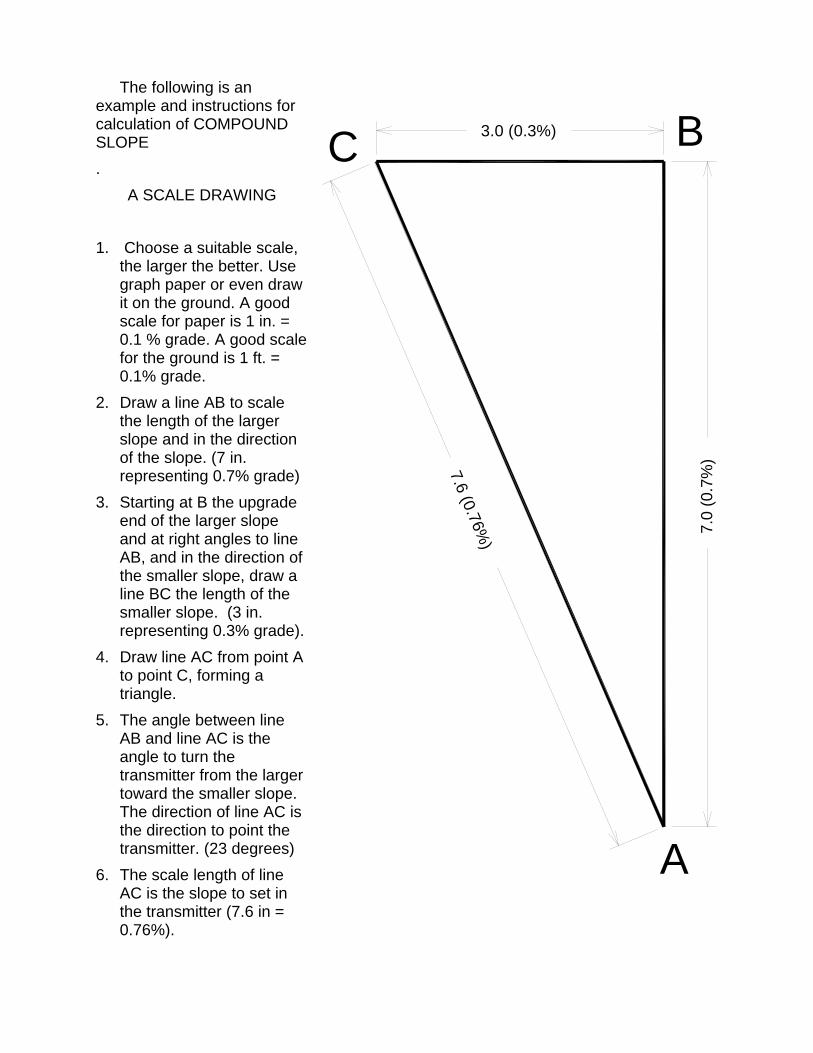
The following is an example and instructions for calculation of COMPOUND SLOPE .
A SCALE DRAWING 1. Choose a suitable scale,
the larger the better. Use graph paper or even draw it on the ground. A good scale for paper is 1 in. = 0.1 % grade. A good scale for the ground is 1 ft. = 0.1% grade.
2. Draw a line AB to scale the length of the larger slope and in the direction of the slope. (7 in. representing 0.7% grade)
3. Starting at B the upgrade end of the larger slope and at right angles to line AB, and in the direction of the smaller slope, draw a line BC the length of the smaller slope. (3 in. representing 0.3% grade).
4. Draw line AC from point A to point C, forming a triangle.
5. The angle between line AB and line AC is the angle to turn the transmitter from the larger toward the smaller slope. The direction of line AC is the direction to point the transmitter. (23 degrees)
6. The scale length of line AC is the slope to set in the transmitter (7.6 in = 0.76%).
3.0 (0.3%)
7.6 (0.76%)
C
7.0
(0.7
%)
A
B
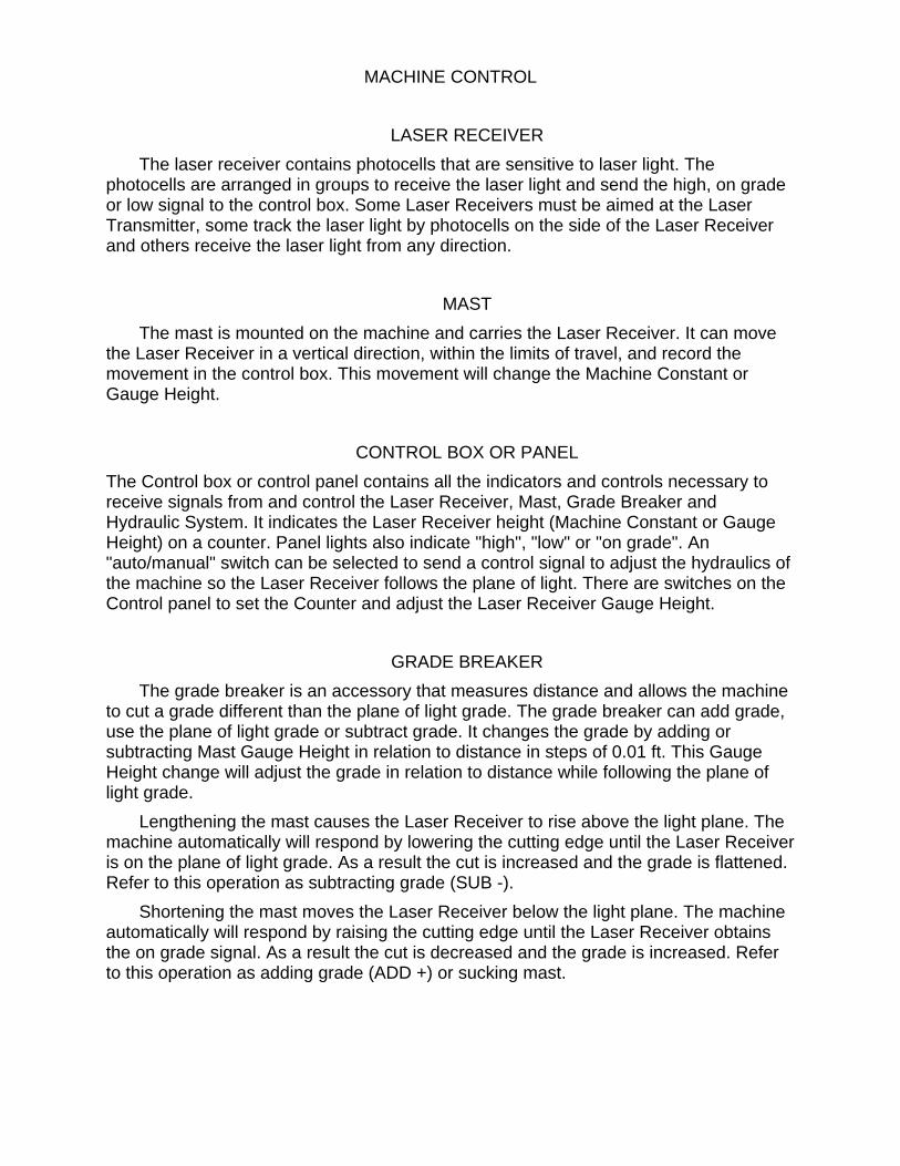
MACHINE CONTROL
LASER RECEIVER The laser receiver contains photocells that are sensitive to laser light. The
photocells are arranged in groups to receive the laser light and send the high, on grade or low signal to the control box. Some Laser Receivers must be aimed at the Laser Transmitter, some track the laser light by photocells on the side of the Laser Receiver and others receive the laser light from any direction.
MAST The mast is mounted on the machine and carries the Laser Receiver. It can move
the Laser Receiver in a vertical direction, within the limits of travel, and record the movement in the control box. This movement will change the Machine Constant or Gauge Height.
CONTROL BOX OR PANEL The Control box or control panel contains all the indicators and controls necessary to receive signals from and control the Laser Receiver, Mast, Grade Breaker and Hydraulic System. It indicates the Laser Receiver height (Machine Constant or Gauge Height) on a counter. Panel lights also indicate "high", "low" or "on grade". An "auto/manual" switch can be selected to send a control signal to adjust the hydraulics of the machine so the Laser Receiver follows the plane of light. There are switches on the Control panel to set the Counter and adjust the Laser Receiver Gauge Height.
GRADE BREAKER The grade breaker is an accessory that measures distance and allows the machine
to cut a grade different than the plane of light grade. The grade breaker can add grade, use the plane of light grade or subtract grade. It changes the grade by adding or subtracting Mast Gauge Height in relation to distance in steps of 0.01 ft. This Gauge Height change will adjust the grade in relation to distance while following the plane of light grade.
Lengthening the mast causes the Laser Receiver to rise above the light plane. The machine automatically will respond by lowering the cutting edge until the Laser Receiver is on the plane of light grade. As a result the cut is increased and the grade is flattened. Refer to this operation as subtracting grade (SUB -).
Shortening the mast moves the Laser Receiver below the light plane. The machine automatically will respond by raising the cutting edge until the Laser Receiver obtains the on grade signal. As a result the cut is decreased and the grade is increased. Refer to this operation as adding grade (ADD +) or sucking mast.
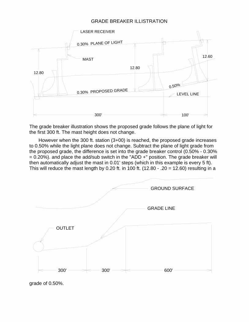
GRADE BREAKER ILLISTRATION
0.50%
12.80
12.60
0.30% PROPOSED GRADE
12.80
300'
0.30% PLANE OF LIGHT
LASER RECEIVER
MAST
100'
LEVEL LINE
The grade breaker illustration shows the proposed grade follows the plane of light for the first 300 ft. The mast height does not change.
However when the 300 ft. station (3+00) is reached, the proposed grade increases to 0.50% while the light plane does not change. Subtract the plane of light grade from the proposed grade, the difference is set into the grade breaker control (0.50% - 0.30% = 0.20%). and place the add/sub switch in the "ADD +" position. The grade breaker will then automatically adjust the mast in 0.01' steps (which in this example is every 5 ft). This will reduce the mast length by 0.20 ft. in 100 ft. (12.80 - .20 = 12.60) resulting in a
grade of 0.50%.
GRADE LINE
GROUND SURFACE
300' 300' 600'
OUTLET
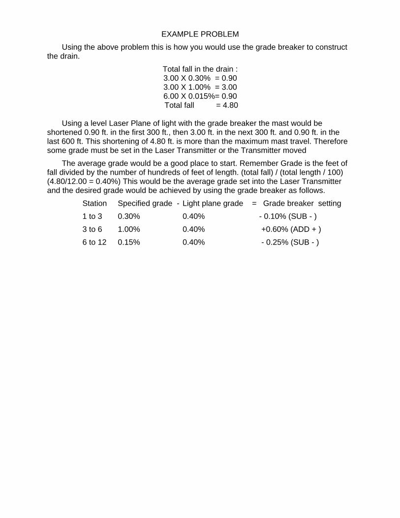
EXAMPLE PROBLEM Using the above problem this is how you would use the grade breaker to construct
the drain. Total fall in the drain : 3.00 X 0.30% = 0.90 3.00 X 1.00% = 3.00 6.00 X 0.015%= 0.90 Total fall = 4.80
Using a level Laser Plane of light with the grade breaker the mast would be
shortened 0.90 ft. in the first 300 ft., then 3.00 ft. in the next 300 ft. and 0.90 ft. in the last 600 ft. This shortening of 4.80 ft. is more than the maximum mast travel. Therefore some grade must be set in the Laser Transmitter or the Transmitter moved
The average grade would be a good place to start. Remember Grade is the feet of fall divided by the number of hundreds of feet of length. (total fall) / (total length / 100) (4.80/12.00 = 0.40%) This would be the average grade set into the Laser Transmitter and the desired grade would be achieved by using the grade breaker as follows.
Station Specified grade - Light plane grade = Grade breaker setting 1 to 3 0.30% 0.40% - 0.10% (SUB - ) 3 to 6 1.00% 0.40% +0.60% (ADD + ) 6 to 12 0.15% 0.40% - 0.25% (SUB - )
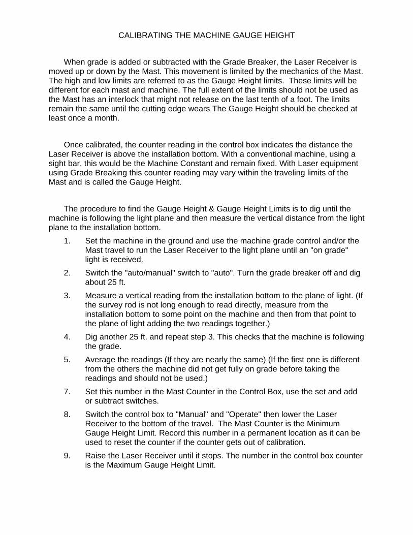
CALIBRATING THE MACHINE GAUGE HEIGHT
When grade is added or subtracted with the Grade Breaker, the Laser Receiver is moved up or down by the Mast. This movement is limited by the mechanics of the Mast. The high and low limits are referred to as the Gauge Height limits. These limits will be different for each mast and machine. The full extent of the limits should not be used as the Mast has an interlock that might not release on the last tenth of a foot. The limits remain the same until the cutting edge wears The Gauge Height should be checked at least once a month.
Once calibrated, the counter reading in the control box indicates the distance the Laser Receiver is above the installation bottom. With a conventional machine, using a sight bar, this would be the Machine Constant and remain fixed. With Laser equipment using Grade Breaking this counter reading may vary within the traveling limits of the Mast and is called the Gauge Height.
The procedure to find the Gauge Height & Gauge Height Limits is to dig until the machine is following the light plane and then measure the vertical distance from the light plane to the installation bottom.
1. Set the machine in the ground and use the machine grade control and/or the Mast travel to run the Laser Receiver to the light plane until an "on grade" light is received.
2. Switch the "auto/manual" switch to "auto". Turn the grade breaker off and dig about 25 ft.
3. Measure a vertical reading from the installation bottom to the plane of light. (If the survey rod is not long enough to read directly, measure from the installation bottom to some point on the machine and then from that point to the plane of light adding the two readings together.)
4. Dig another 25 ft. and repeat step 3. This checks that the machine is following the grade.
5. Average the readings (If they are nearly the same) (If the first one is different from the others the machine did not get fully on grade before taking the readings and should not be used.)
7. Set this number in the Mast Counter in the Control Box, use the set and add or subtract switches.
8. Switch the control box to "Manual" and "Operate" then lower the Laser Receiver to the bottom of the travel. The Mast Counter is the Minimum Gauge Height Limit. Record this number in a permanent location as it can be used to reset the counter if the counter gets out of calibration.
9. Raise the Laser Receiver until it stops. The number in the control box counter is the Maximum Gauge Height Limit.
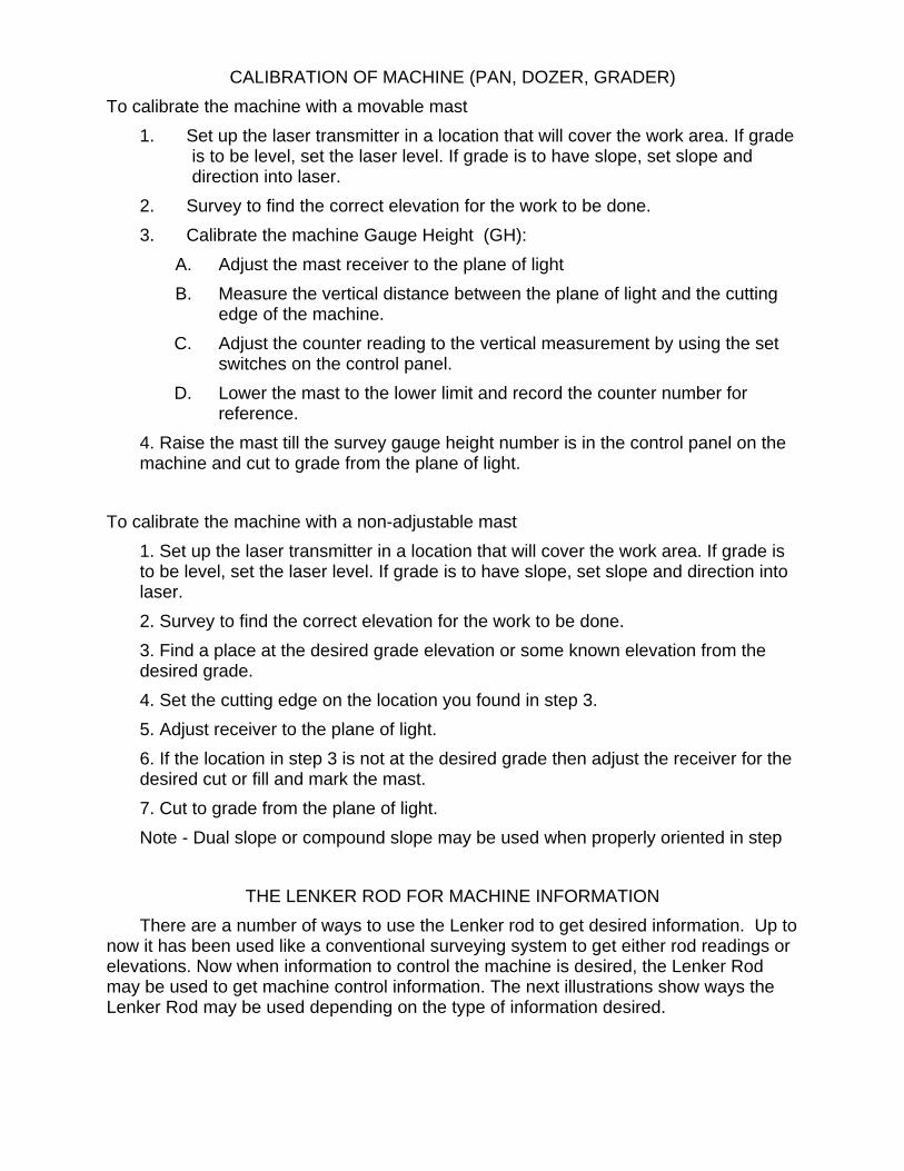
CALIBRATION OF MACHINE (PAN, DOZER, GRADER) To calibrate the machine with a movable mast
1. Set up the laser transmitter in a location that will cover the work area. If grade is to be level, set the laser level. If grade is to have slope, set slope and direction into laser.
2. Survey to find the correct elevation for the work to be done. 3. Calibrate the machine Gauge Height (GH):
A. Adjust the mast receiver to the plane of light B. Measure the vertical distance between the plane of light and the cutting
edge of the machine. C. Adjust the counter reading to the vertical measurement by using the set
switches on the control panel. D. Lower the mast to the lower limit and record the counter number for
reference. 4. Raise the mast till the survey gauge height number is in the control panel on the machine and cut to grade from the plane of light.
To calibrate the machine with a non-adjustable mast
1. Set up the laser transmitter in a location that will cover the work area. If grade is to be level, set the laser level. If grade is to have slope, set slope and direction into laser. 2. Survey to find the correct elevation for the work to be done. 3. Find a place at the desired grade elevation or some known elevation from the desired grade. 4. Set the cutting edge on the location you found in step 3. 5. Adjust receiver to the plane of light. 6. If the location in step 3 is not at the desired grade then adjust the receiver for the desired cut or fill and mark the mast. 7. Cut to grade from the plane of light. Note - Dual slope or compound slope may be used when properly oriented in step
THE LENKER ROD FOR MACHINE INFORMATION
There are a number of ways to use the Lenker rod to get desired information. Up to now it has been used like a conventional surveying system to get either rod readings or elevations. Now when information to control the machine is desired, the Lenker Rod may be used to get machine control information. The next illustrations show ways the Lenker Rod may be used depending on the type of information desired.
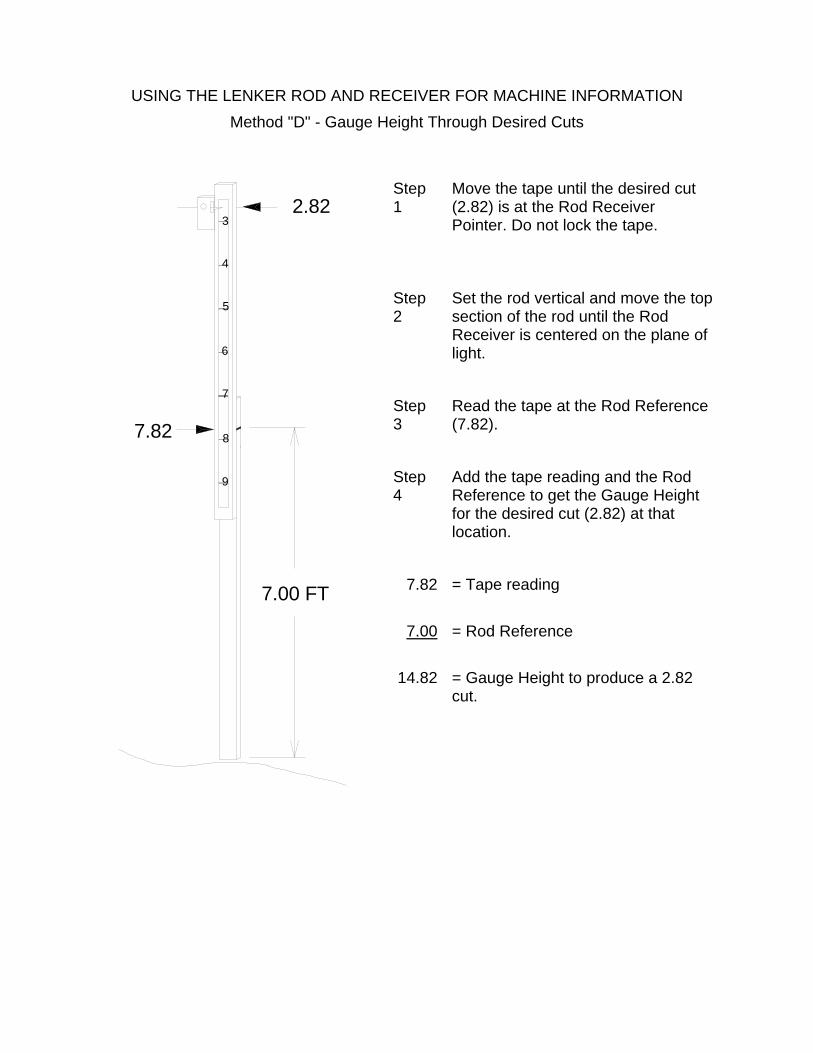
USING THE LENKER ROD AND RECEIVER FOR MACHINE INFORMATION
Method "D" - Gauge Height Through Desired Cuts
Step 1
Move the tape until the desired cut (2.82) is at the Rod Receiver Pointer. Do not lock the tape.
Step 2
Set the rod vertical and move the top section of the rod until the Rod Receiver is centered on the plane of light.
Step 3
Read the tape at the Rod Reference (7.82).
Step 4
Add the tape reading and the Rod Reference to get the Gauge Height for the desired cut (2.82) at that location.
7.82 = Tape reading
7.00 = Rod Reference
14.82 = Gauge Height to produce a 2.82 cut.
7.82
7.00 FT
9
6
8
7
4
5
2.823
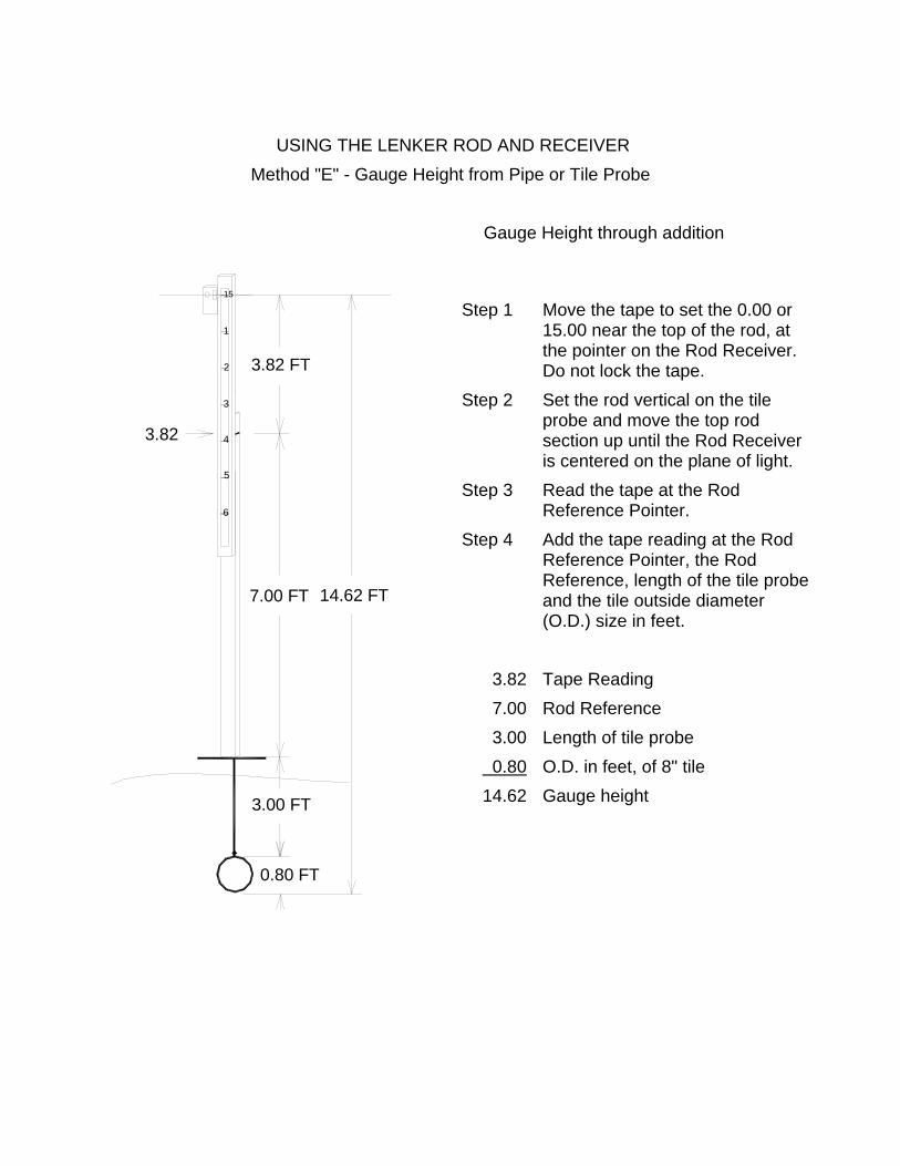
USING THE LENKER ROD AND RECEIVER
Method "E" - Gauge Height from Pipe or Tile Probe
Gauge Height through addition
3.82
6
5
4
3
2
15
1
14.62 FT
0.80 FT
3.00 FT
7.00 FT
3.82 FT
Step 1 Move the tape to set the 0.00 or 15.00 near the top of the rod, at the pointer on the Rod Receiver. Do not lock the tape.
Step 2 Set the rod vertical on the tile probe and move the top rod section up until the Rod Receiver is centered on the plane of light.
Step 3 Read the tape at the Rod Reference Pointer.
Step 4 Add the tape reading at the Rod Reference Pointer, the Rod Reference, length of the tile probe and the tile outside diameter (O.D.) size in feet.
3.82 Tape Reading 7.00 Rod Reference 3.00 Length of tile probe
0.80 O.D. in feet, of 8" tile 14.62 Gauge height
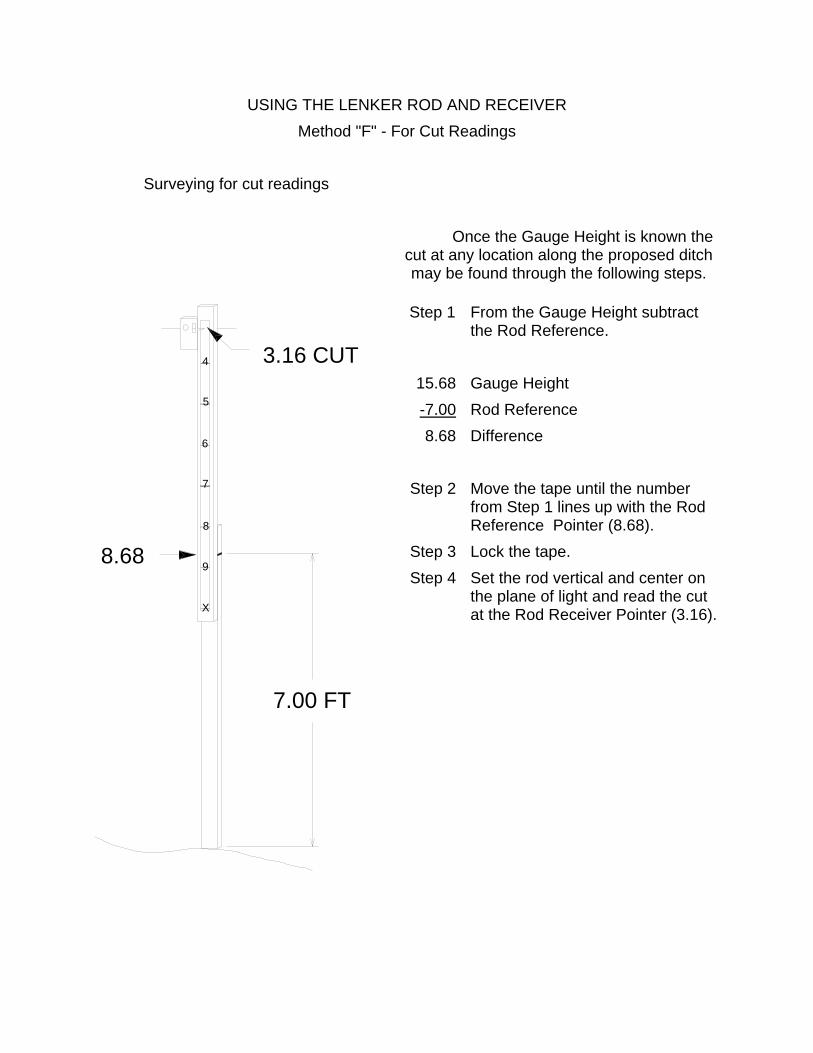
USING THE LENKER ROD AND RECEIVER Method "F" - For Cut Readings
Surveying for cut readings
Once the Gauge Height is known the
cut at any location along the proposed ditch may be found through the following steps.
8.68
6
9
X
7
8
5
4 3.16 CUT
7.00 FT
Step 1 From the Gauge Height subtract the Rod Reference.
15.68 Gauge Height -7.00 Rod Reference 8.68 Difference
Step 2 Move the tape until the number
from Step 1 lines up with the Rod Reference Pointer (8.68).
Step 3 Lock the tape. Step 4 Set the rod vertical and center on
the plane of light and read the cut at the Rod Receiver Pointer (3.16).
DEFINITIONS OF TERMS USED IN SURVEYING AZIMUTH RING - A ring located on the command post used to figure compound
grades. BACK SIGHT (BS) (+) - A level rod reading taken at a point of known elevation It is the
first reading taken on a bench mark or turning point immediately after the initial or new setup. The BACK SIGHT is added to the elevation to obtain the Height of Instrument (H.I.).
BEEPER - see ROD RECEIVER BENCHMARK (BM) - A benchmark is a point of known elevation of a permanent nature.
It may be elevation above Sea Level or assumed at some convenient number (usually 100.00). A permanent bench mark will be a brass pin or cap set in concrete, a long metal stake driven in the ground or a certain point on a concrete bridge or other solid object. A temporary benchmark, (TBM) needed for only a few weeks until a job is completed could be a wood stake or a nail in a tree or post. Benchmark locations should be accurately described in the field book and plans, so a person who had never been in the area could locate them.
COMPOUND SLOPE - Is the maximum slope between two right angle slopes. CONTOUR INTERVAL - The difference in elevation represented by each contour line
on a map. CONTOUR LINE - A line drawn on a map that connects points of the same elevation. CONTOUR MAP - A map on which irregularities of land surface are shown by contour
lines, the relative spacing of the lines indicating the relative slope of the surface CONTROL BOX - An interface on a machine to receive signals from a receiver, mast,
grade breaker or slope meter and indicate to the operator various information also to send signals to control points on the machine if desired.
CROSS ARM - A short horizontal bar attached to a stake a known distance from the bottom of the proposed ditch.
CROSS SECTION - A profile taken at right angles from the station line. CUT - The distance from the ground surface to the bottom of the trench or grade
elevation CUT CARD - A pocket size card with heading and columns , which has column to
record rod readings, survey gauge height and figure cuts and grade breaker settings
DATUM - A level surface with respect to which elevations are established This may be sea level or an imaginary line under or on the ground surface.
DETECTOR - see ROD RECEIVER DETECTOR POINTER - see ROD RECEIVER POINTER DIFFERENTIAL LEVELING - A method of leveling used to find the difference in
elevation between points.
DITCH BOTTOM (DB) - The lowest point in the ditch or the normal low water level. ELEVATION (ELEV) - The height of a point in relation to Datum whether sea level or
assumed. FIELD BOOK - A book used as a permanent record of surveying. FIELD NOTES - Notes taken in the field and recorded in the field book as the survey is
carried out. They are a record of the survey and as such should be complete, identifying the survey by title, including location and purpose, identification of party members and duties, type of equipment used, date and weather conditions.
FORESIGHT (FS) (-) - A rod reading taken at a point of unknown elevation The foresight is subtracted from the height of instrument (H.I.) to find the elevation. (HI - FS = ELEV)
GAUGE HEIGHT - The vertical distance from the sight bar or receiver to the bottom of the finished cut
GRADE - SLOPE - The rate of rise or fall along a specified line. Grade is the same as slope and is usually expressed in percent (feet of rise or fall in 100 feet of horizontal distance).
GRADE BREAKER - A distance measuring mechanism attached to a machine that can change gauge height in relation to distance.
GRADE ELEVATION - The desired elevation of a trench, ditch or surface. GUARD STAKE - A stake or marker placed beside a hub stake to locate, protect and
identify the hub stake. HEIGHT OF INSTRUMENT (HI) - The elevation of the line of sight of a surveying
instrument or a level plane of light. It is found by adding the BACK SIGHT (+) to the elevation of the bench mark or turning point. (ELEV + BS = HI)
HUB STAKE - A short stake driven almost flush with the ground to mark elevations at stations
LASER DETECTOR - see ROD RECEIVER. LASER RECEIVER - An instrument that indicates the location of a laser light, usually
attached to a machine to indicate or control the grading of the machine. LASER TRANSMITTER - TRANSMITTER - A source of laser light that rotates to
generate a plane of light, used as a reference to determine elevations or cuts or control a machine.
LASER TRANSMITTER SLOPE - The amount of slope on the plane of light LATERAL IDENTIFICATION CARD - see CUT CARD LENKER ROD - A level rod used in surveying that has a graduated movable tape or
ribbon. The Lenker rod can be used to read elevations directly. Use of this rod reduces the amount of calculations needed in entering notes or elevations.
LEVEL - An instrument used to establish a true horizontal line of sight.
LEVEL ROD - A rod used in surveying to determine the distance from a line of sight or laser light to a point. Usually graduated in feet, tenths and hundreds.
MACHINE CONSTANT - see GAUGE HEIGHT MAST - An adjustable support for a Laser Receiver, controlled or monitored through the
control box. PROFILE - A vertical section of the ground surface along the line of survey. PROFILE LEVELING - A method of finding the elevations of a series of points at
measured horizontal distances along a specified line. RANGE POLE - A long pole with feet painted alternating red - white, used to mark
points that must be seen from a distance. RIBBON LOCK - see TAPE LOCK. ROD RECEIVER - DETECTOR - LASER DETECTOR - SENTRY - BEEPER - A laser
receiver of small size that may be attached to a level rod ROD RECEIVER POINTER - The pointer on the ROD RECEIVER where the plane of
light would intersect and rod readings are taken. ROD REFERENCE POINT - The marker for the distance from the bottom of the Lenker
rod usually even feet. This is the point where rod readings will sometimes be taken and added to the reference amount for that rod. Also used as a reference mark to determine if the tape lock has loosened allowing the tape to move
SENTRY - see ROD RECEIVER SLOPE - see GRADE STATION (STA.) - Points along a line of survey, usually 100 ft. intervals The first station
is zero. Stations are usually marked with a hub stake and guard stake, paint or flag. Rod readings are taken at stations.
SURVEY CUT - Is the difference between the survey gauge height (SGH) at the beginning of the ditch, and the (SGH) of the station.
SURVEY GAUGE HEIGHT (SGH.) -Vertical distance from a tilted plane of light to the ground
TAPE LOCK - RIBBON LOCK - Clamp that locks the ribbon or tape on a Lenker rod, so that it does not move in relation to the bottom section of the rod - The: Reference point reading remains constant.
TILTED PLANE - When the Laser Transmitter has slope on the light plane. TRIPOD - A three-leg support for a Level or Laser Transmitter TURNING POINT (TP) - A turning point is a firm object such as a hub stake, stone,
fence post or axe head so that the elevation will not change while the instrument or transmitter is being moved. A point on which a foresight (-) rod reading is taken to obtain the elevation and on which a BACK SIGHT (+) rod reading is taken after the instrument is moved to a new location.

Tab for Topographic Mapping
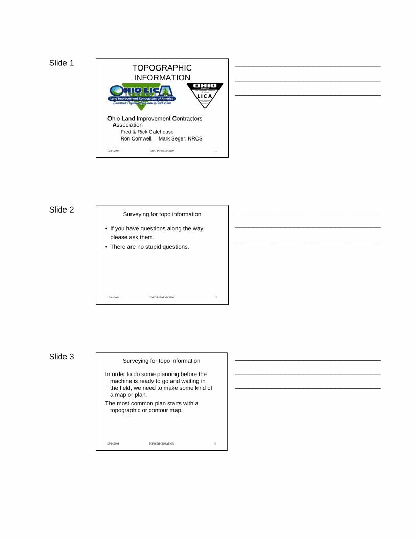
Slide 1
12/14/2004 TOPO INFORMATION 1
TOPOGRAPHIC INFORMATION
Ohio Land Improvement Contractors Association
Fred & Rick GalehouseRon Cornwell, Mark Seger, NRCS
________________________________
________________________________
________________________________
Slide 2
12/14/2004 TOPO INFORMATION 2
Surveying for topo information
• If you have questions along the way please ask them.
• There are no stupid questions.
________________________________
________________________________
________________________________
Slide 3
12/14/2004 TOPO INFORMATION 3
Surveying for topo information
In order to do some planning before the machine is ready to go and waiting in the field, we need to make some kind of a map or plan.
The most common plan starts with a topographic or contour map.
________________________________
________________________________
________________________________
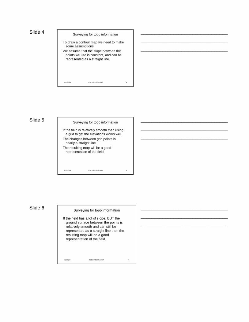
Slide 4
12/14/2004 TOPO INFORMATION 4
Surveying for topo information
To draw a contour map we need to make some assumptions.
We assume that the slope between the points we use is constant, and can be represented as a straight line.
________________________________
________________________________
________________________________
Slide 5
12/14/2004 TOPO INFORMATION 5
Surveying for topo information
If the field is relatively smooth then using a grid to get the elevations works well.
The changes between grid points is nearly a straight line.
The resulting map will be a good representation of the field.
________________________________
________________________________
________________________________
Slide 6
12/14/2004 TOPO INFORMATION 6
Surveying for topo information
If the field has a lot of slope, BUT the ground surface between the points is relatively smooth and can still be represented as a straight line then the resulting map will be a good representation of the field.
________________________________
________________________________
________________________________
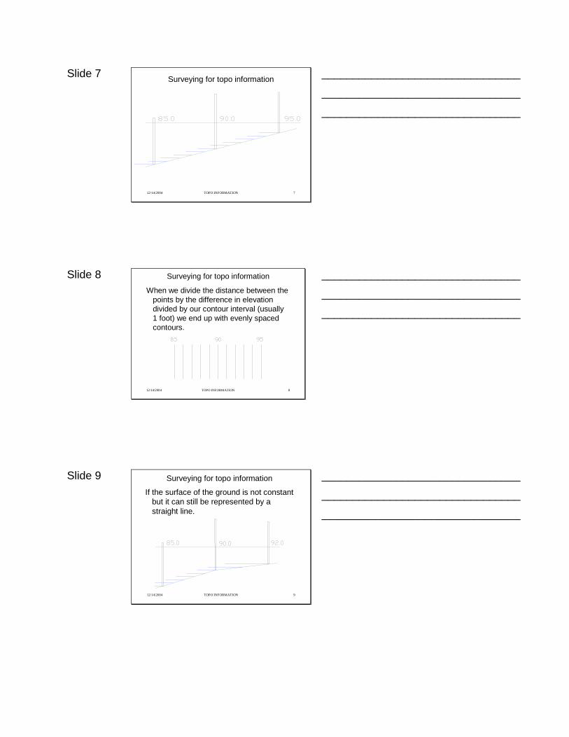
Slide 7
12/14/2004 TOPO INFORMATION 7
Surveying for topo information ________________________________
________________________________
________________________________
Slide 8
12/14/2004 TOPO INFORMATION 8
Surveying for topo information
When we divide the distance between the points by the difference in elevation divided by our contour interval (usually 1 foot) we end up with evenly spaced contours.
________________________________
________________________________
________________________________
Slide 9
12/14/2004 TOPO INFORMATION 9
Surveying for topo information
If the surface of the ground is not constant but it can still be represented by a straight line.
________________________________
________________________________
________________________________
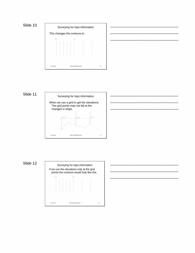
Slide 10
12/14/2004 TOPO INFORMATION 10
Surveying for topo information
This changes the contours to
________________________________
________________________________
________________________________
Slide 11
12/14/2004 TOPO INFORMATION 11
Surveying for topo information
When we use a grid to get the elevations. The grid points may not fall at the changes in slope.
________________________________
________________________________
________________________________
Slide 12
12/14/2004 TOPO INFORMATION 12
Surveying for topo informationIf we use the elevations only at the grid
points the contours would look like this.
________________________________
________________________________
________________________________
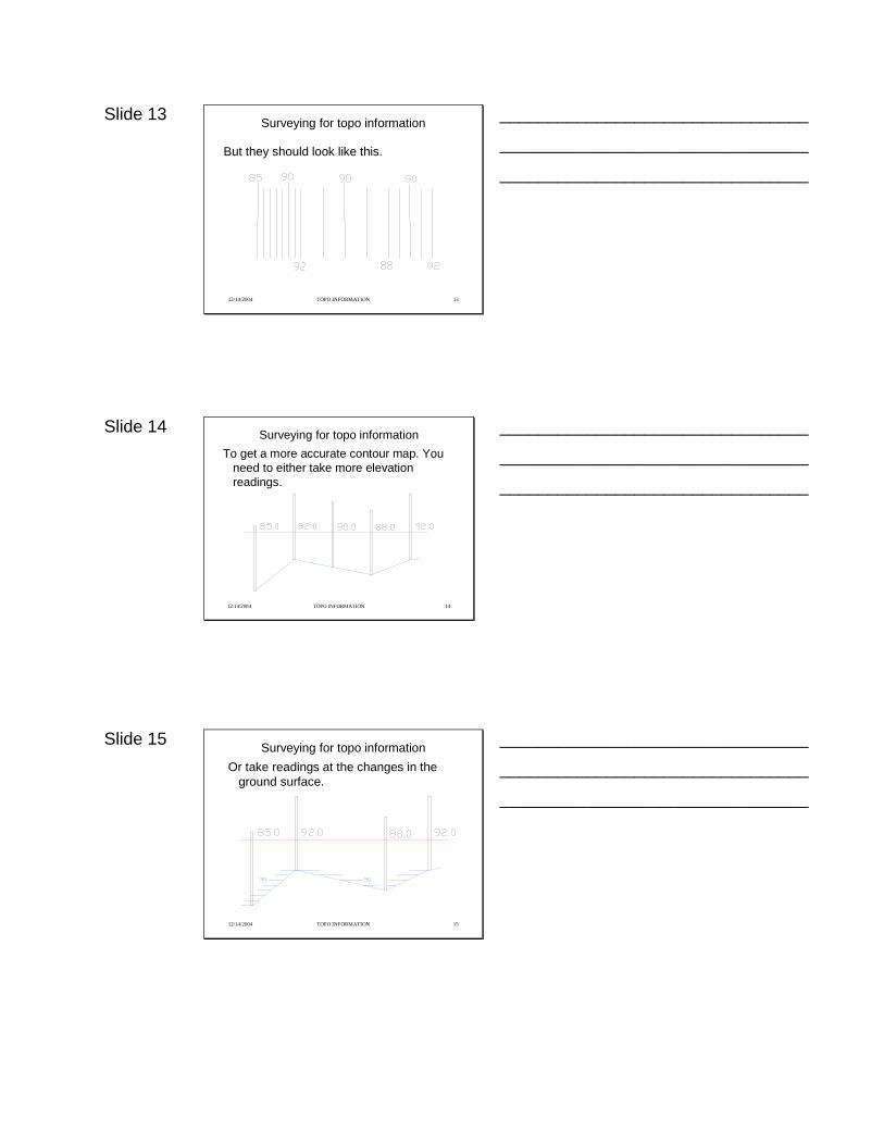
Slide 13
12/14/2004 TOPO INFORMATION 13
Surveying for topo information
But they should look like this.
________________________________
________________________________
________________________________
Slide 14
12/14/2004 TOPO INFORMATION 14
Surveying for topo informationTo get a more accurate contour map. You
need to either take more elevation readings.
________________________________
________________________________
________________________________
Slide 15
12/14/2004 TOPO INFORMATION 15
Surveying for topo informationOr take readings at the changes in the
ground surface.
________________________________
________________________________
________________________________
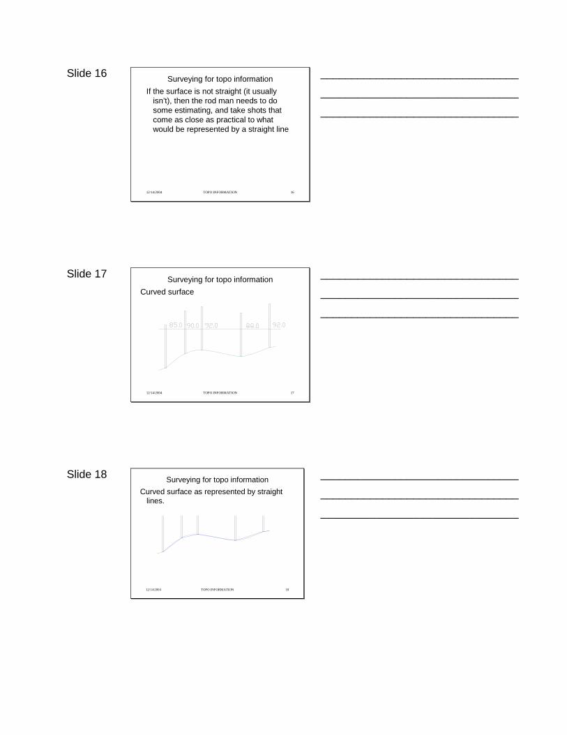
Slide 16
12/14/2004 TOPO INFORMATION 16
Surveying for topo informationIf the surface is not straight (it usually
isn’t), then the rod man needs to do some estimating, and take shots that come as close as practical to what would be represented by a straight line
________________________________
________________________________
________________________________
Slide 17
12/14/2004 TOPO INFORMATION 17
Surveying for topo informationCurved surface
________________________________
________________________________
________________________________
Slide 18
12/14/2004 TOPO INFORMATION 18
Surveying for topo informationCurved surface as represented by straight
lines.
________________________________
________________________________
________________________________
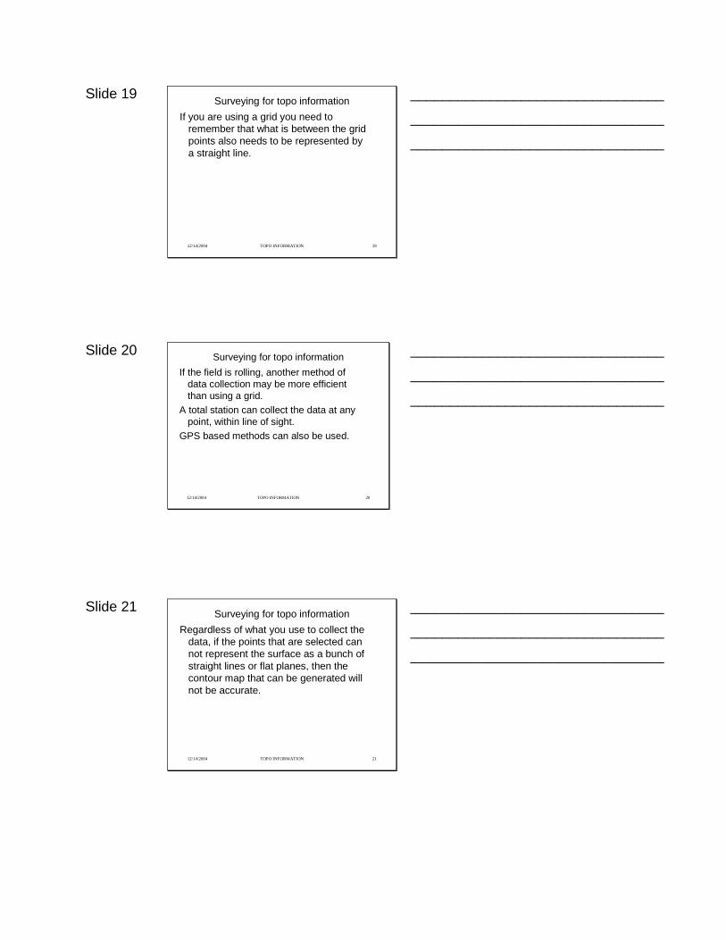
Slide 19
12/14/2004 TOPO INFORMATION 19
Surveying for topo informationIf you are using a grid you need to
remember that what is between the grid points also needs to be represented by a straight line.
________________________________
________________________________
________________________________
Slide 20
12/14/2004 TOPO INFORMATION 20
Surveying for topo informationIf the field is rolling, another method of
data collection may be more efficient than using a grid.
A total station can collect the data at any point, within line of sight.
GPS based methods can also be used.
________________________________
________________________________
________________________________
Slide 21
12/14/2004 TOPO INFORMATION 21
Surveying for topo informationRegardless of what you use to collect the
data, if the points that are selected can not represent the surface as a bunch of straight lines or flat planes, then the contour map that can be generated will not be accurate.
________________________________
________________________________
________________________________
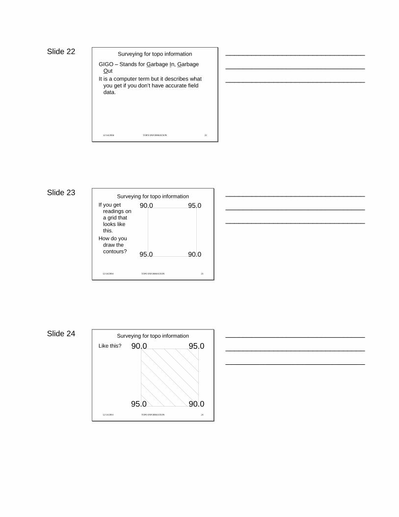
Slide 22
12/14/2004 TOPO INFORMATION 22
Surveying for topo information
GIGO – Stands for Garbage In, Garbage Out
It is a computer term but it describes what you get if you don’t have accurate field data.
________________________________
________________________________
________________________________
Slide 23
12/14/2004 TOPO INFORMATION 23
Surveying for topo informationIf you get
readings on a grid that looks like this.
How do you draw the contours?
90.0 95.0
90.095.0
________________________________
________________________________
________________________________
Slide 24
12/14/2004 TOPO INFORMATION 24
Surveying for topo information
Like this?
95.0
90.0
90.0
95.0
________________________________
________________________________
________________________________
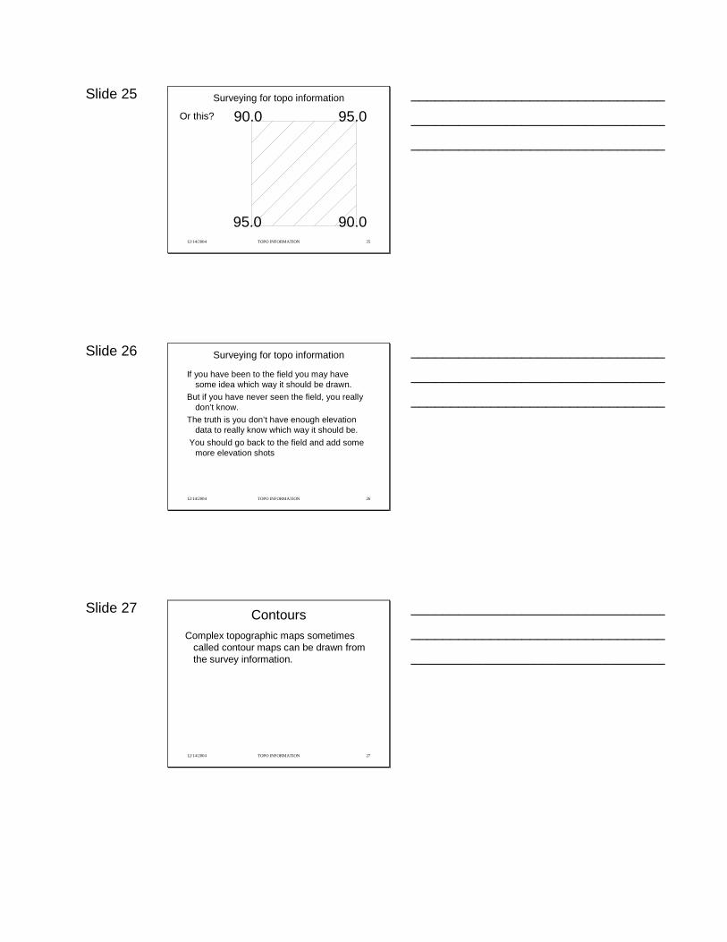
Slide 25
12/14/2004 TOPO INFORMATION 25
Surveying for topo information
Or this?
95.0
90.0
90.0
95.0
________________________________
________________________________
________________________________
Slide 26
12/14/2004 TOPO INFORMATION 26
Surveying for topo information
If you have been to the field you may have some idea which way it should be drawn.
But if you have never seen the field, you really don’t know.
The truth is you don’t have enough elevation data to really know which way it should be.
You should go back to the field and add some more elevation shots
________________________________
________________________________
________________________________
Slide 27
12/14/2004 TOPO INFORMATION 27
ContoursComplex topographic maps sometimes
called contour maps can be drawn from the survey information.
________________________________
________________________________
________________________________
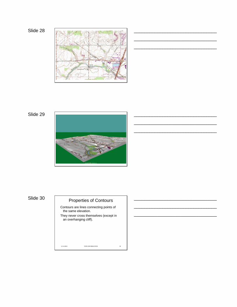
Slide 28
12/14/2004 TOPO INFORMATION 28
________________________________
________________________________
________________________________
Slide 29
12/14/2004 TOPO INFORMATION 29
________________________________
________________________________
________________________________
Slide 30
12/14/2004 TOPO INFORMATION 30
Properties of ContoursContours are lines connecting points of
the same elevation.They never cross themselves (except in
an overhanging cliff).
________________________________
________________________________
________________________________
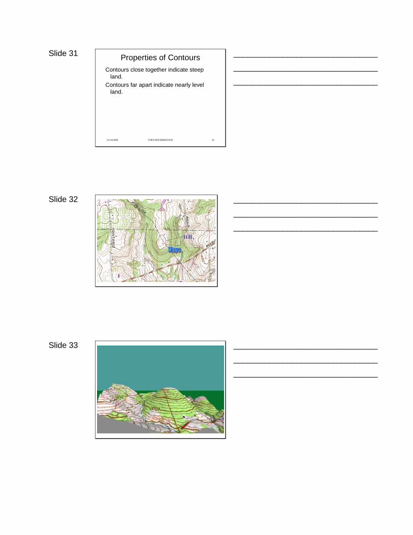
Slide 31
12/14/2004 TOPO INFORMATION 31
Properties of ContoursContours close together indicate steep
land.Contours far apart indicate nearly level
land.
________________________________
________________________________
________________________________
Slide 32
12/14/2004 TOPO INFORMATION 32
Hill
________________________________
________________________________
________________________________
Slide 33
12/14/2004 TOPO INFORMATION 33
________________________________
________________________________
________________________________
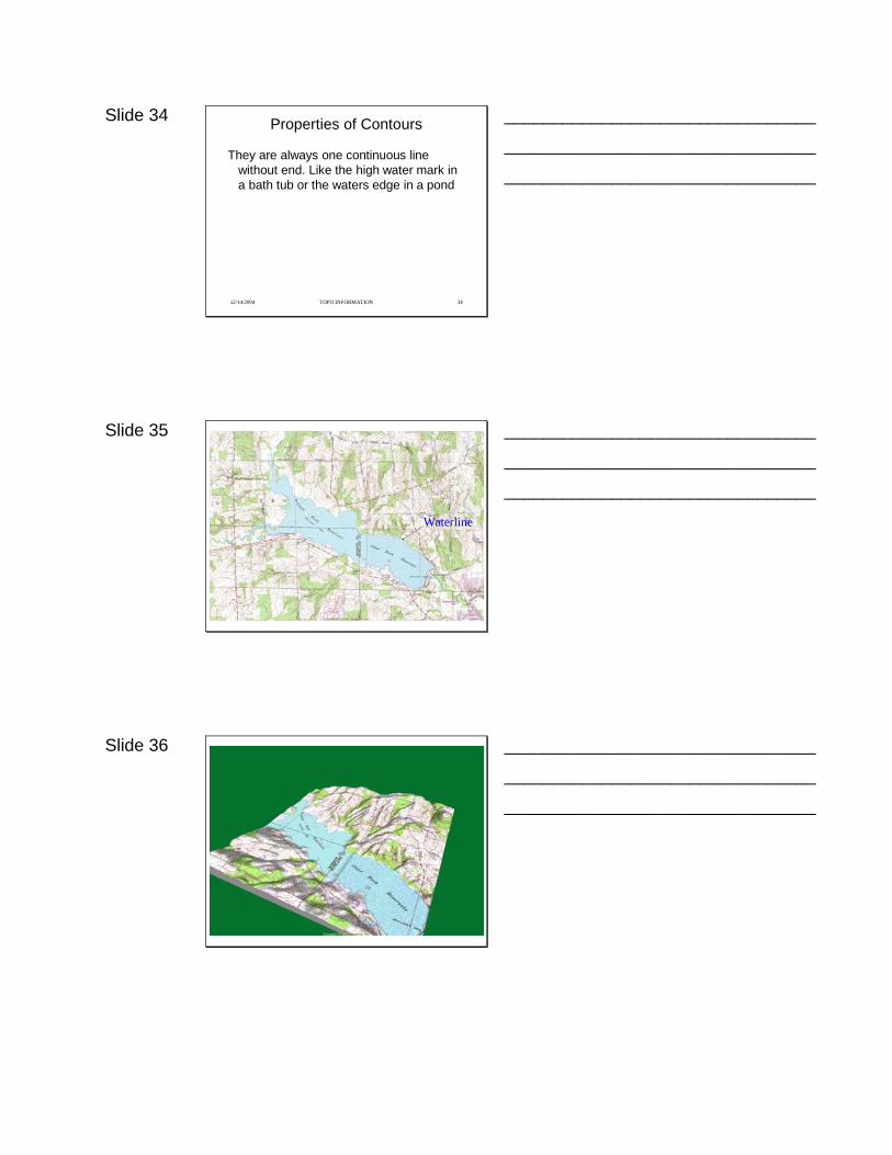
Slide 34
12/14/2004 TOPO INFORMATION 34
Properties of Contours
They are always one continuous line without end. Like the high water mark in a bath tub or the waters edge in a pond
________________________________
________________________________
________________________________
Slide 35
12/14/2004 TOPO INFORMATION 35
Waterline
________________________________
________________________________
________________________________
Slide 36
12/14/2004 TOPO INFORMATION 36
________________________________
________________________________
________________________________
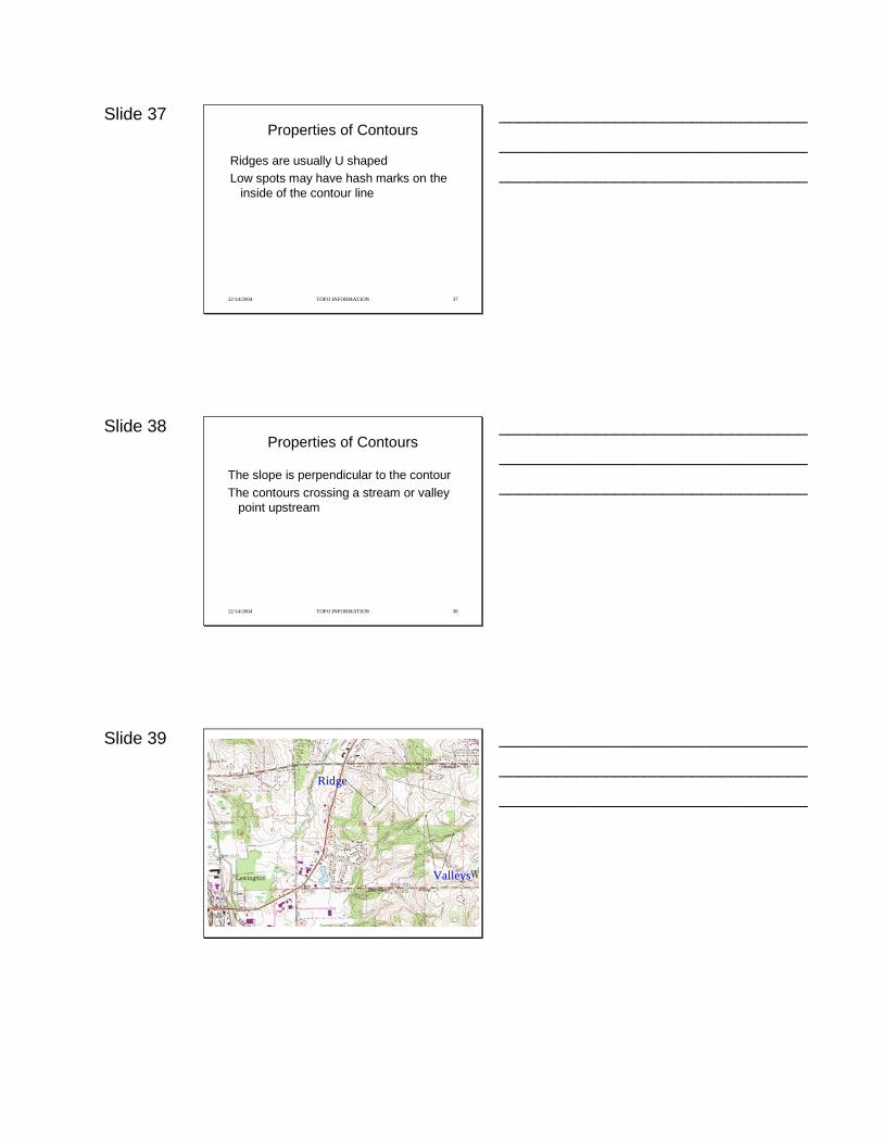
Slide 37
12/14/2004 TOPO INFORMATION 37
Properties of Contours
Ridges are usually U shapedLow spots may have hash marks on the
inside of the contour line
________________________________
________________________________
________________________________
Slide 38
12/14/2004 TOPO INFORMATION 38
Properties of Contours
The slope is perpendicular to the contourThe contours crossing a stream or valley
point upstream
________________________________
________________________________
________________________________
Slide 39
12/14/2004 TOPO INFORMATION 39
Valleys
Ridge
________________________________
________________________________
________________________________
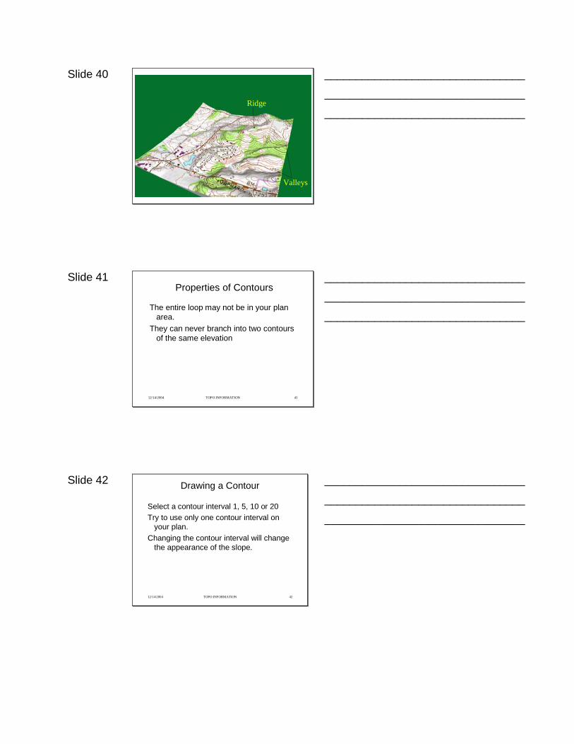
Slide 40
12/14/2004 TOPO INFORMATION 40
Valleys
Ridge
________________________________
________________________________
________________________________
Slide 41
12/14/2004 TOPO INFORMATION 41
Properties of Contours
The entire loop may not be in your plan area.
They can never branch into two contours of the same elevation
________________________________
________________________________
________________________________
Slide 42
12/14/2004 TOPO INFORMATION 42
Drawing a Contour
Select a contour interval 1, 5, 10 or 20Try to use only one contour interval on
your plan.Changing the contour interval will change
the appearance of the slope.
________________________________
________________________________
________________________________
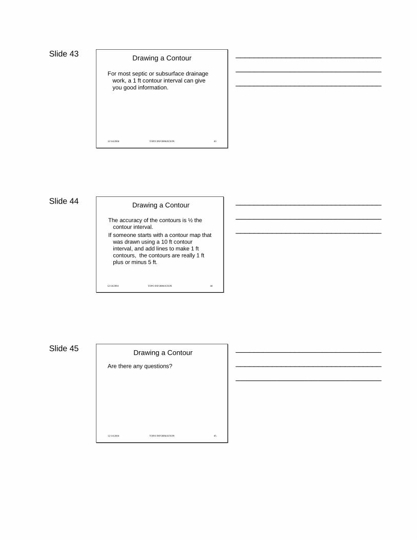
Slide 43
12/14/2004 TOPO INFORMATION 43
Drawing a Contour
For most septic or subsurface drainage work, a 1 ft contour interval can give you good information.
________________________________
________________________________
________________________________
Slide 44
12/14/2004 TOPO INFORMATION 44
Drawing a Contour
The accuracy of the contours is ½ the contour interval.
If someone starts with a contour map that was drawn using a 10 ft contour interval, and add lines to make 1 ft contours, the contours are really 1 ft plus or minus 5 ft.
________________________________
________________________________
________________________________
Slide 45
12/14/2004 TOPO INFORMATION 45
Drawing a Contour
Are there any questions?
________________________________
________________________________
________________________________
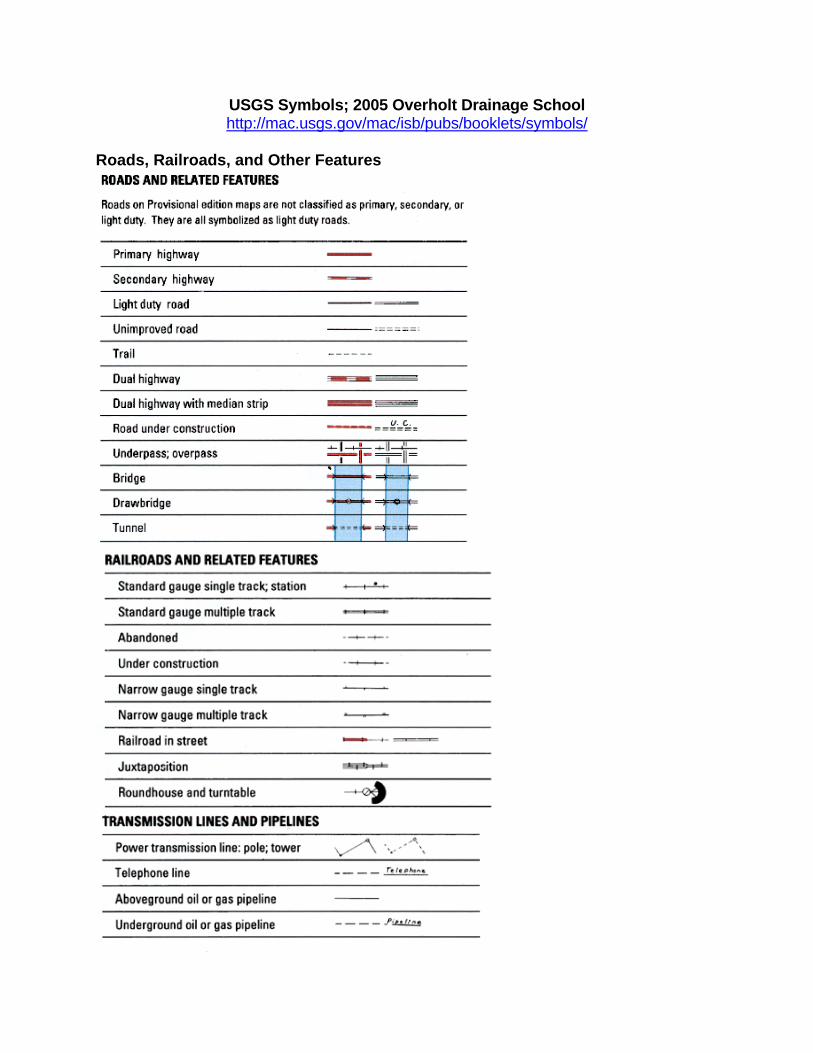
USGS Symbols; 2005 Overholt Drainage School http://mac.usgs.gov/mac/isb/pubs/booklets/symbols/
Roads, Railroads, and Other Features
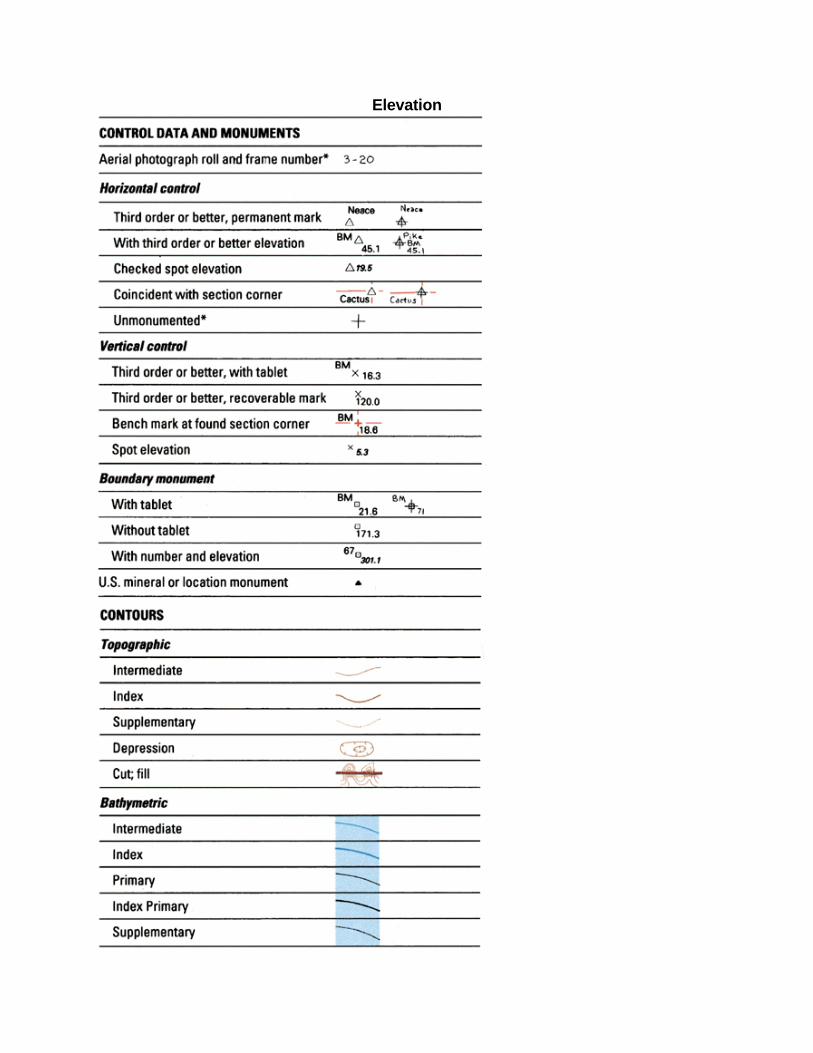
Elevation
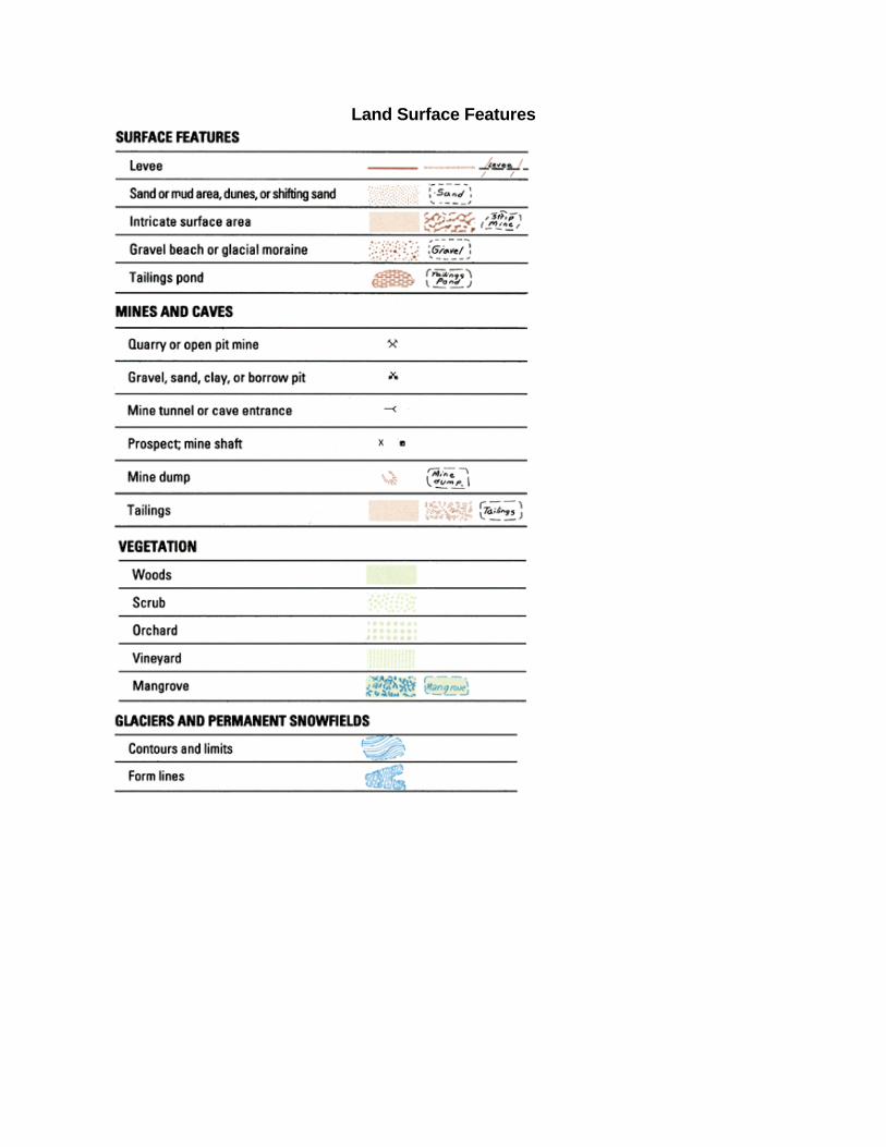
Land Surface Features
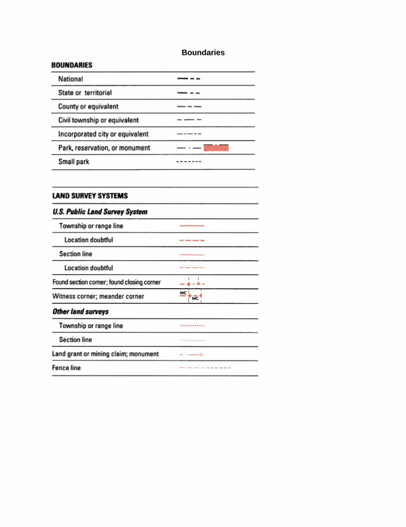
Boundaries
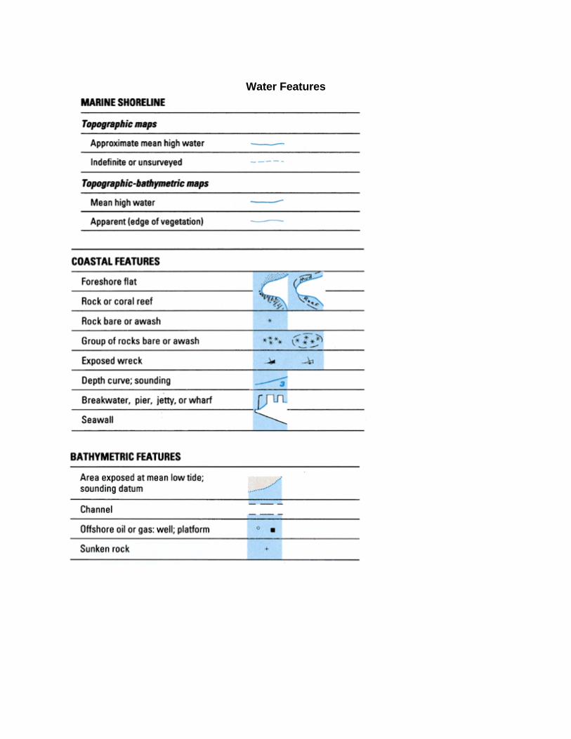
Water Features
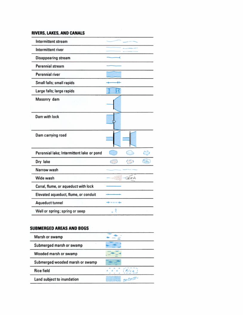
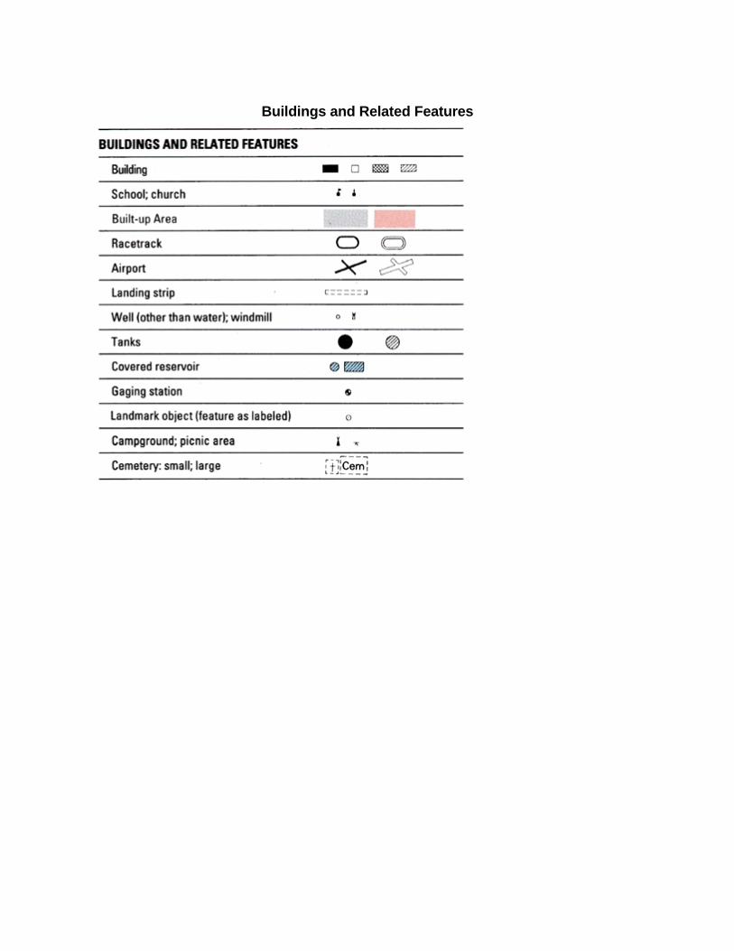
Buildings and Related Features

Tab for Drawing Contours
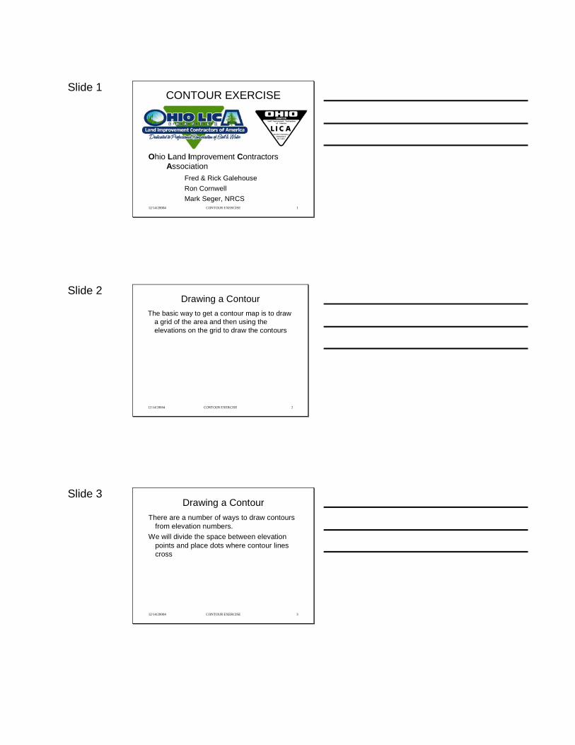
Slide 1
12/14/20004 CONTOUR EXERCISE 1
CONTOUR EXERCISE
Ohio Land Improvement Contractors Association
Fred & Rick GalehouseRon CornwellMark Seger, NRCS
Slide 2
12/14/20004 CONTOUR EXERCISE 2
Drawing a ContourThe basic way to get a contour map is to draw
a grid of the area and then using the elevations on the grid to draw the contours
Slide 3
12/14/20004 CONTOUR EXERCISE 3
Drawing a ContourThere are a number of ways to draw contours
from elevation numbers. We will divide the space between elevation
points and place dots where contour lines cross
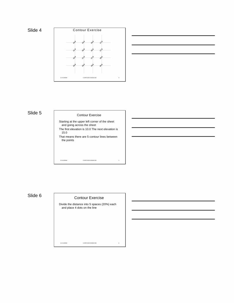
Slide 4
12/14/20004 CONTOUR EXERCISE 4
10.0
15.0 16.0 17.0
17.516.516.011.0
12.0
17.0 17.5 18.5
15.0
18.0 19.5 20.5
Contour Exercise
Slide 5
12/14/20004 CONTOUR EXERCISE 5
Contour Exercise
Starting at the upper left corner of the sheet and going across the sheet
The first elevation is 10.0 The next elevation is 15.0
That means there are 5 contour lines between the points
Slide 6
12/14/20004 CONTOUR EXERCISE 6
Contour ExerciseDivide the distance into 5 spaces (20%) each
and place 4 dots on the line
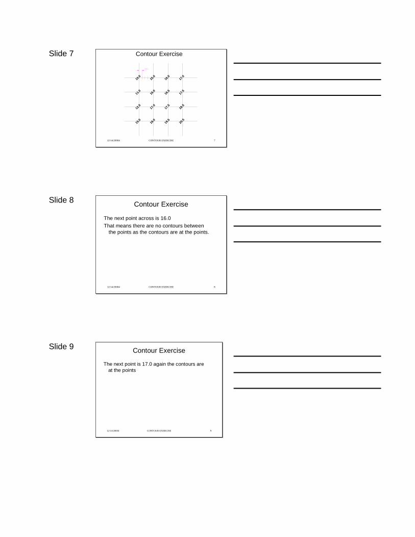
Slide 7
12/14/20004 CONTOUR EXERCISE 7
Contour Exercise
16.0
11.0
12.0
15.0
18.0
17.0
10.0
15.0
17.5
16.5
18.5
20.5
19.5
17.5
17.0
16.0
Slide 8
12/14/20004 CONTOUR EXERCISE 8
Contour Exercise
The next point across is 16.0That means there are no contours between
the points as the contours are at the points.
Slide 9
12/14/20004 CONTOUR EXERCISE 9
Contour Exercise
The next point is 17.0 again the contours are at the points
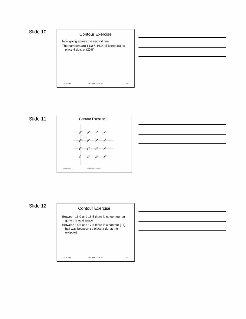
Slide 10
12/14/20004 CONTOUR EXERCISE 10
Contour ExerciseNow going across the second lineThe numbers are 11.0 & 16.0 ( 5 contours) so
place 4 dots at (20%)
Slide 11
12/14/20004 CONTOUR EXERCISE 11
Contour Exercise
16.0
11.0
12.0
15.0
18.0
17.0
10.0
15.0
17.5
16.5
18.5
20.5
19.5
17.5
17.0
16.0
Slide 12
12/14/20004 CONTOUR EXERCISE 12
Contour Exercise
Between 16.0 and 16.5 there is no contour so go to the next space
Between 16.5 and 17.5 there is a contour (17) half way between so place a dot at the midpoint.
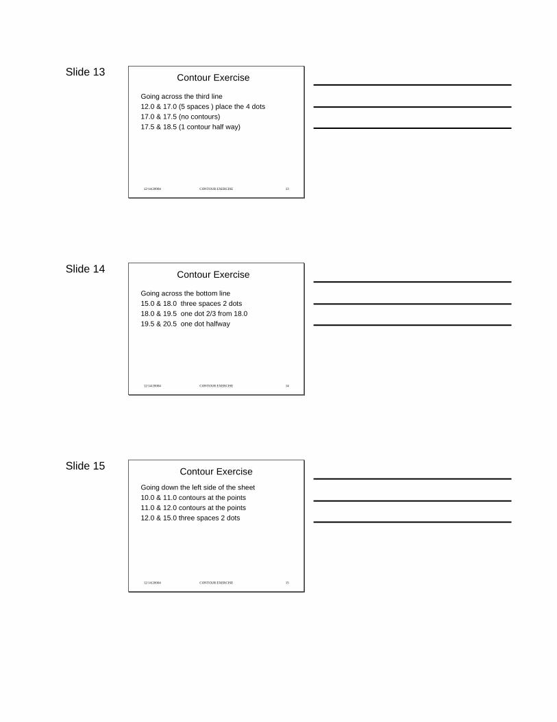
Slide 13
12/14/20004 CONTOUR EXERCISE 13
Contour Exercise
Going across the third line12.0 & 17.0 (5 spaces ) place the 4 dots17.0 & 17.5 (no contours)17.5 & 18.5 (1 contour half way)
Slide 14
12/14/20004 CONTOUR EXERCISE 14
Contour Exercise
Going across the bottom line15.0 & 18.0 three spaces 2 dots18.0 & 19.5 one dot 2/3 from 18.019.5 & 20.5 one dot halfway
Slide 15
12/14/20004 CONTOUR EXERCISE 15
Contour ExerciseGoing down the left side of the sheet10.0 & 11.0 contours at the points11.0 & 12.0 contours at the points12.0 & 15.0 three spaces 2 dots
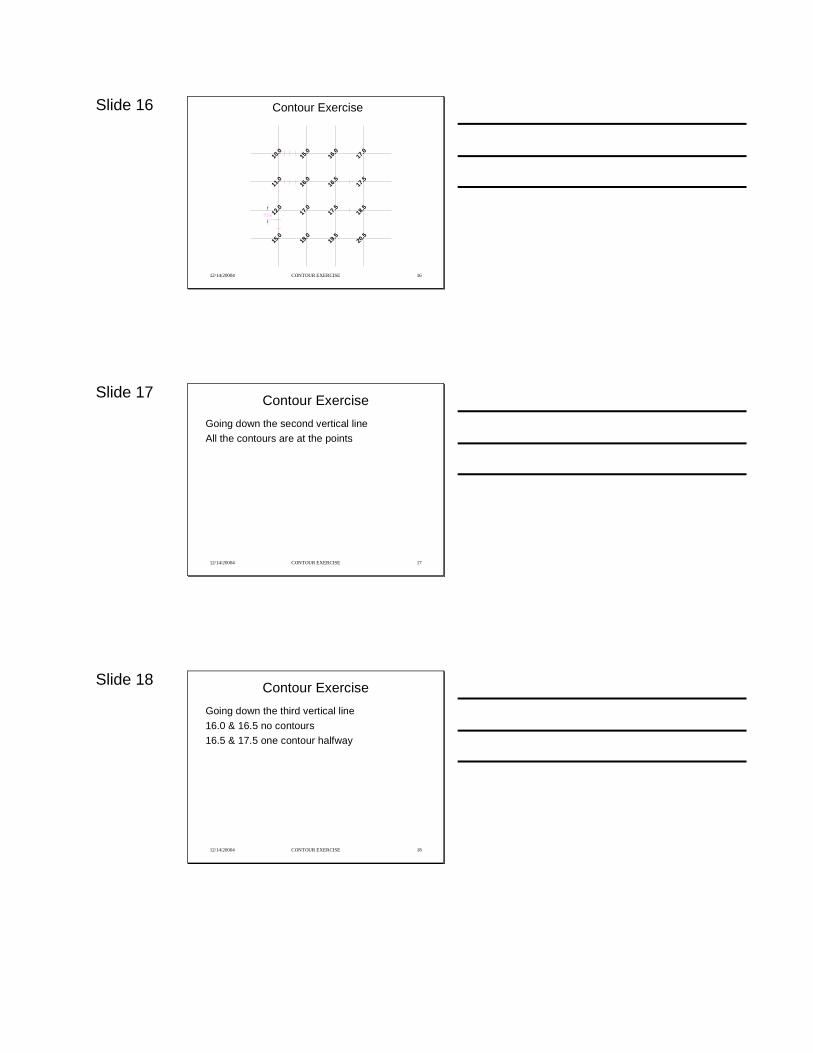
Slide 16
12/14/20004 CONTOUR EXERCISE 16
Contour Exercise
16.0
11.0
12.0
15.0
18.0
17.0
10.0
15.0
17.5
16.5
18.5
20.5
19.5
17.5
17.0
16.0
Slide 17
12/14/20004 CONTOUR EXERCISE 17
Contour ExerciseGoing down the second vertical lineAll the contours are at the points
Slide 18
12/14/20004 CONTOUR EXERCISE 18
Contour ExerciseGoing down the third vertical line16.0 & 16.5 no contours16.5 & 17.5 one contour halfway
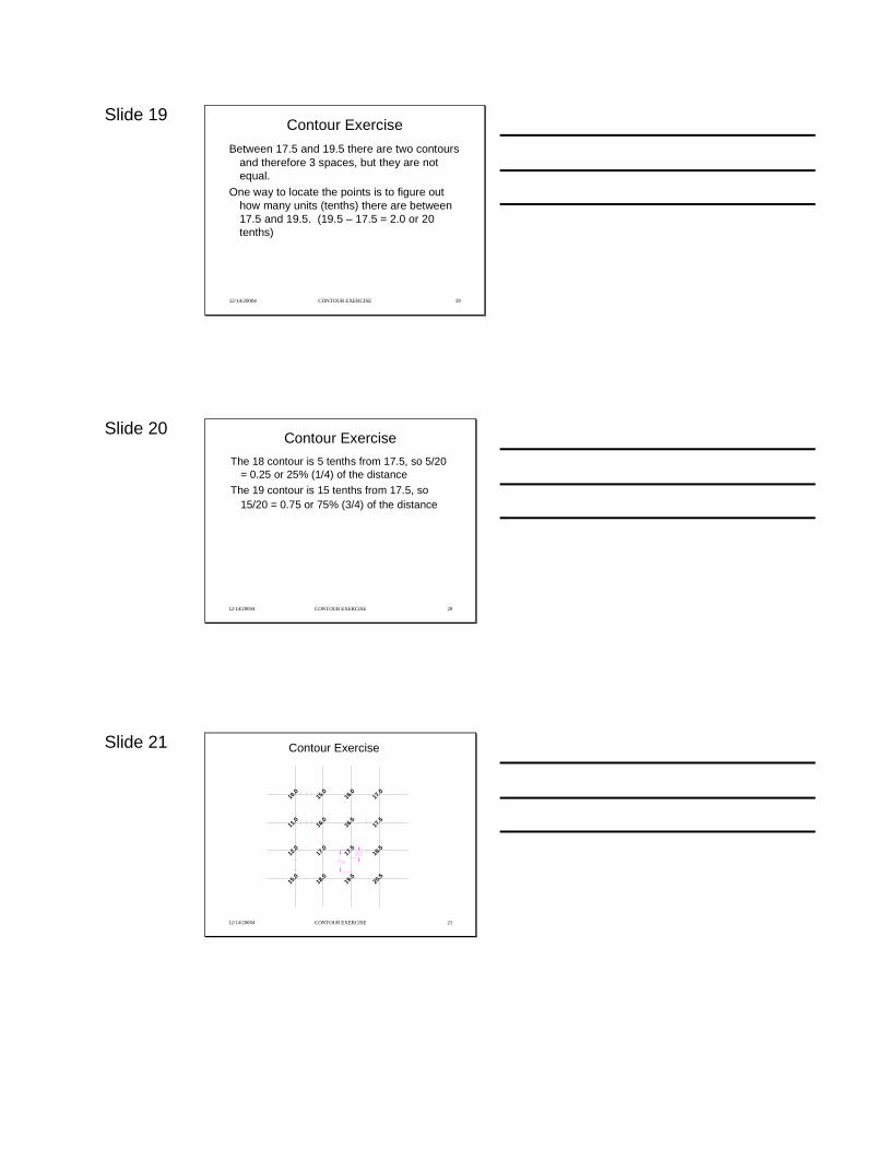
Slide 19
12/14/20004 CONTOUR EXERCISE 19
Contour ExerciseBetween 17.5 and 19.5 there are two contours
and therefore 3 spaces, but they are not equal.
One way to locate the points is to figure out how many units (tenths) there are between 17.5 and 19.5. (19.5 – 17.5 = 2.0 or 20 tenths)
Slide 20
12/14/20004 CONTOUR EXERCISE 20
Contour ExerciseThe 18 contour is 5 tenths from 17.5, so 5/20
= 0.25 or 25% (1/4) of the distanceThe 19 contour is 15 tenths from 17.5, so
15/20 = 0.75 or 75% (3/4) of the distance
Slide 21
12/14/20004 CONTOUR EXERCISE 21
Contour Exercise
16.0
11.0
12.0
15.0
18.0
17.0
10.0
15.0
17.5
16.5
18.5
20.5
19.5
17.5
17.0
16.0
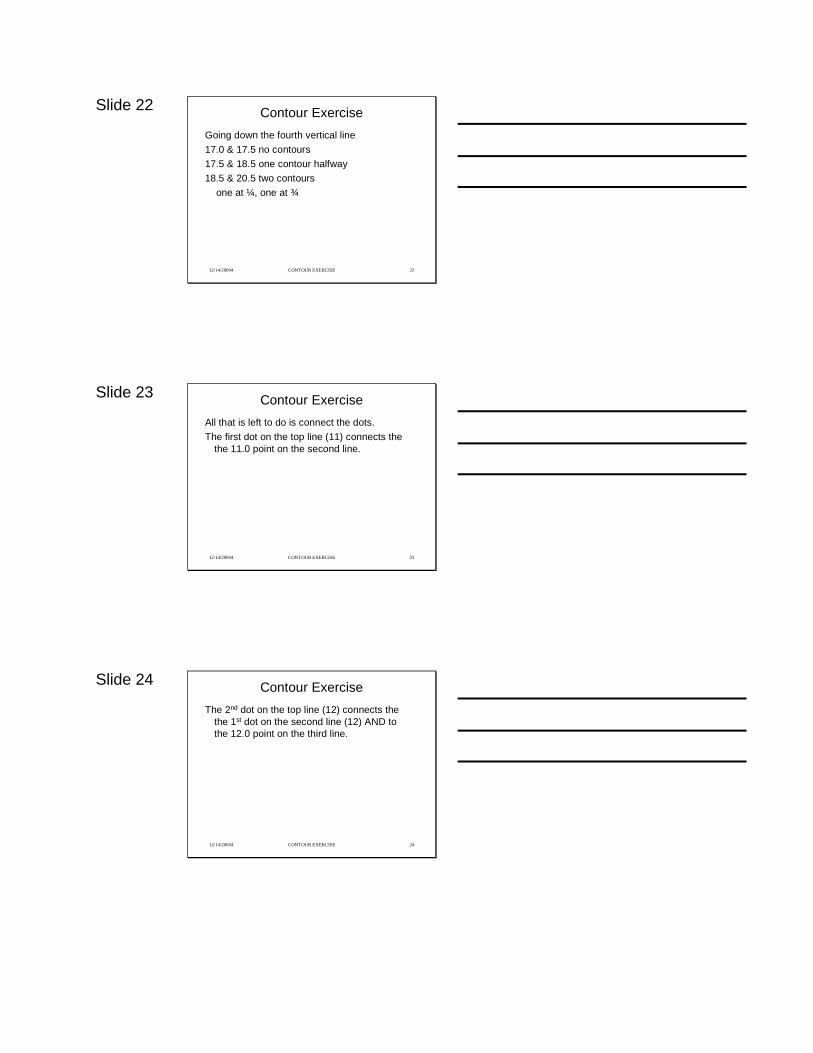
Slide 22
12/14/20004 CONTOUR EXERCISE 22
Contour ExerciseGoing down the fourth vertical line17.0 & 17.5 no contours17.5 & 18.5 one contour halfway18.5 & 20.5 two contours
one at ¼, one at ¾
Slide 23
12/14/20004 CONTOUR EXERCISE 23
Contour ExerciseAll that is left to do is connect the dots.The first dot on the top line (11) connects the
the 11.0 point on the second line.
Slide 24
12/14/20004 CONTOUR EXERCISE 24
Contour ExerciseThe 2nd dot on the top line (12) connects the
the 1st dot on the second line (12) AND to the 12.0 point on the third line.
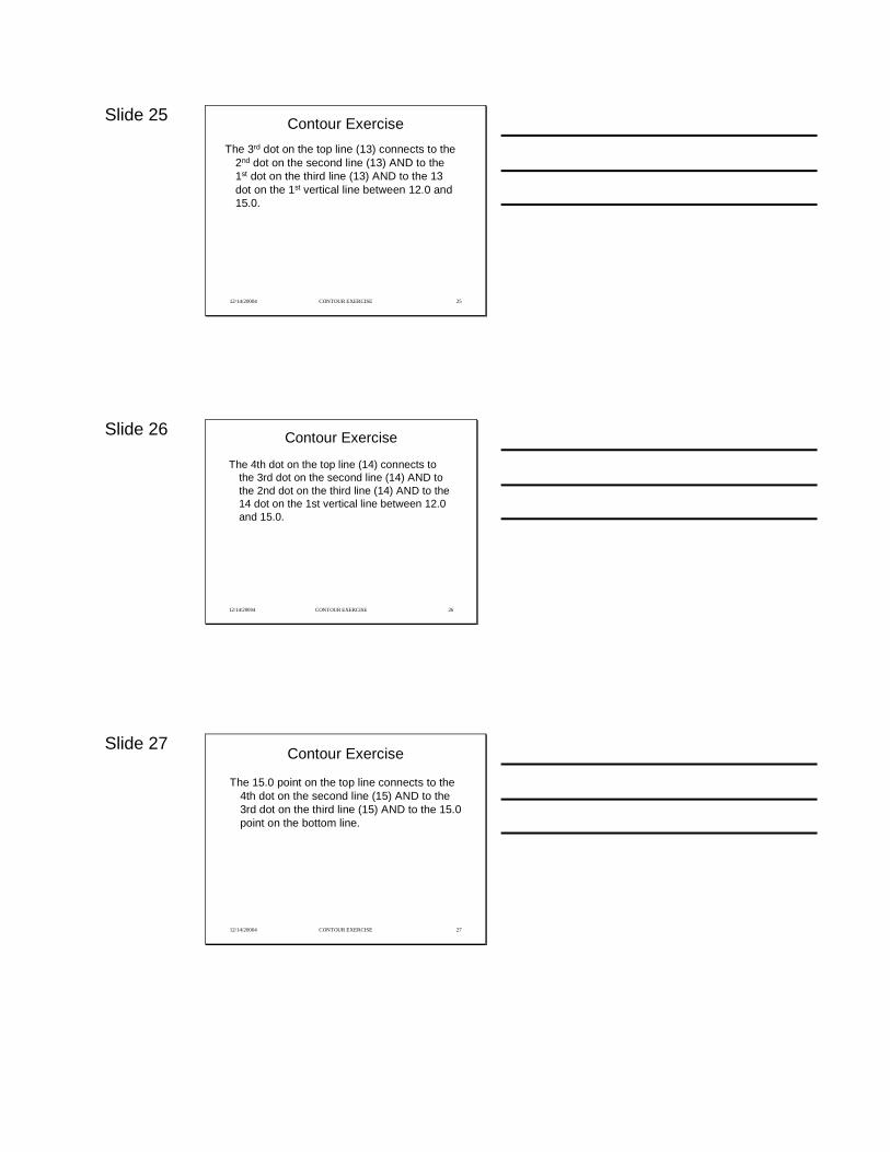
Slide 25
12/14/20004 CONTOUR EXERCISE 25
Contour ExerciseThe 3rd dot on the top line (13) connects to the
2nd dot on the second line (13) AND to the 1st dot on the third line (13) AND to the 13 dot on the 1st vertical line between 12.0 and 15.0.
Slide 26
12/14/20004 CONTOUR EXERCISE 26
Contour Exercise
The 4th dot on the top line (14) connects to the 3rd dot on the second line (14) AND to the 2nd dot on the third line (14) AND to the 14 dot on the 1st vertical line between 12.0 and 15.0.
Slide 27
12/14/20004 CONTOUR EXERCISE 27
Contour Exercise
The 15.0 point on the top line connects to the 4th dot on the second line (15) AND to the 3rd dot on the third line (15) AND to the 15.0 point on the bottom line.
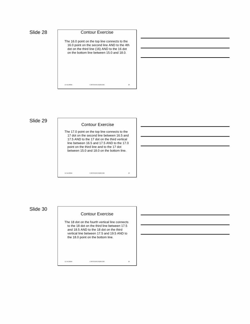
Slide 28
12/14/20004 CONTOUR EXERCISE 28
Contour Exercise
The 16.0 point on the top line connects to the 16.0 point on the second line AND to the 4th dot on the third line (16) AND to the 16 dot on the bottom line between 15.0 and 18.0.
Slide 29
12/14/20004 CONTOUR EXERCISE 29
Contour ExerciseThe 17.0 point on the top line connects to the
17 dot on the second line between 16.5 and 17.5 AND to the 17 dot on the third vertical line between 16.5 and 17.5 AND to the 17.0 point on the third line and to the 17 dot between 15.0 and 18.0 on the bottom line.
Slide 30
12/14/20004 CONTOUR EXERCISE 30
Contour Exercise
The 18 dot on the fourth vertical line connects to the 18 dot on the third line between 17.5 and 18.5 AND to the 18 dot on the third vertical line between 17.5 and 19.5 AND to the 18.0 point on the bottom line.
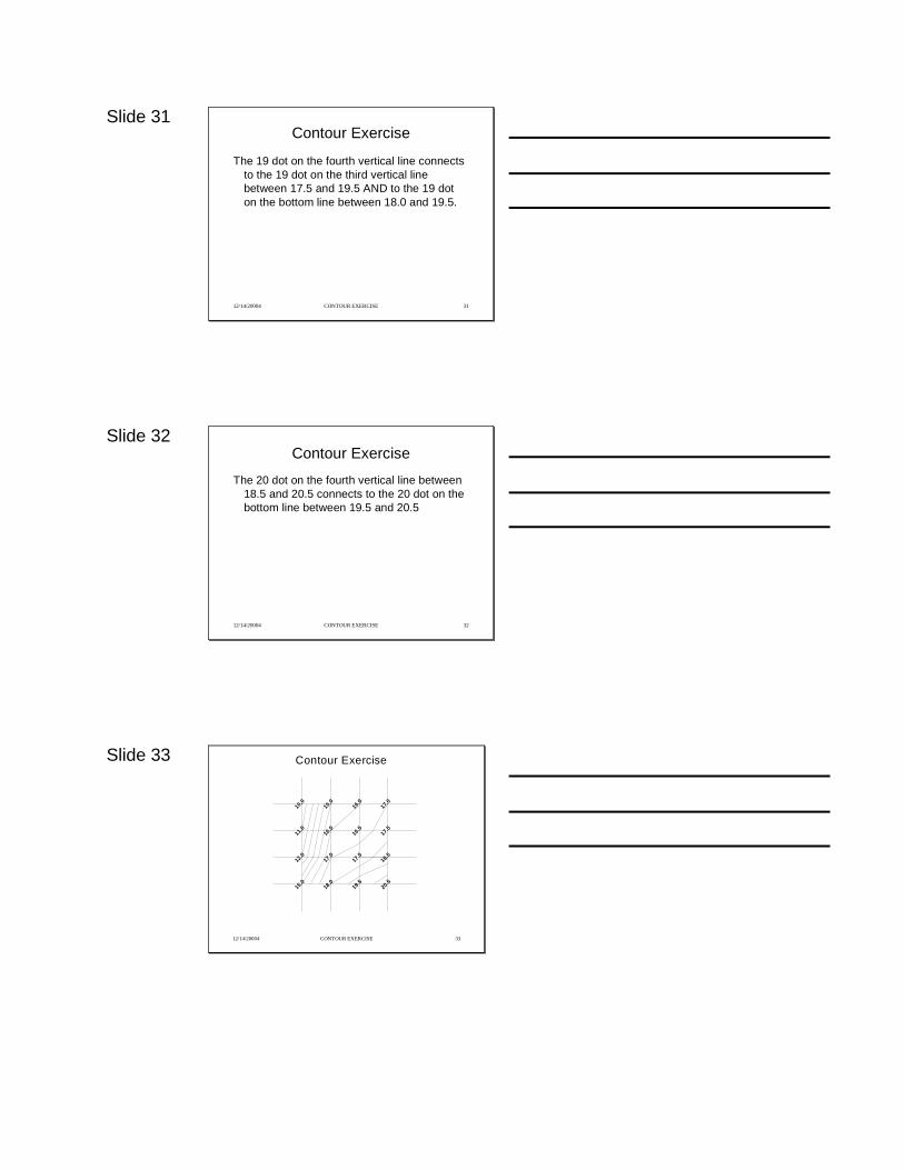
Slide 31
12/14/20004 CONTOUR EXERCISE 31
Contour Exercise
The 19 dot on the fourth vertical line connects to the 19 dot on the third vertical line between 17.5 and 19.5 AND to the 19 dot on the bottom line between 18.0 and 19.5.
Slide 32
12/14/20004 CONTOUR EXERCISE 32
Contour Exercise
The 20 dot on the fourth vertical line between 18.5 and 20.5 connects to the 20 dot on the bottom line between 19.5 and 20.5
Slide 33
12/14/20004 CONTOUR EXERCISE 33
Contour Exercise
11.0
16.0
15.0
12.0
18.0
17.0
10.0
15.0
16.5
17.5
20.5
18.5
19.5
17.5
17.0
16.0
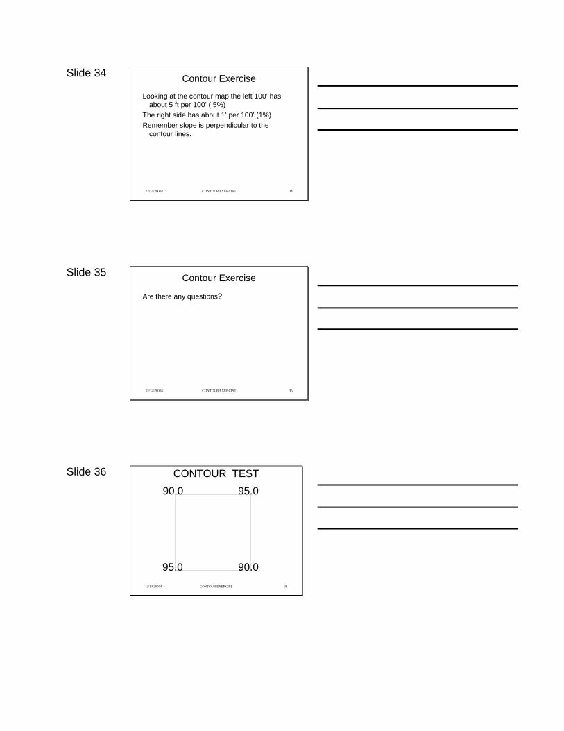
Slide 34
12/14/20004 CONTOUR EXERCISE 34
Contour Exercise
Looking at the contour map the left 100’ has about 5 ft per 100’ ( 5%)
The right side has about 1’ per 100’ (1%)Remember slope is perpendicular to the
contour lines.
Slide 35
12/14/20004 CONTOUR EXERCISE 35
Contour Exercise
Are there any questions?
Slide 36
12/14/20004 CONTOUR EXERCISE 36
CONTOUR TEST90.0 95.0
90.095.0
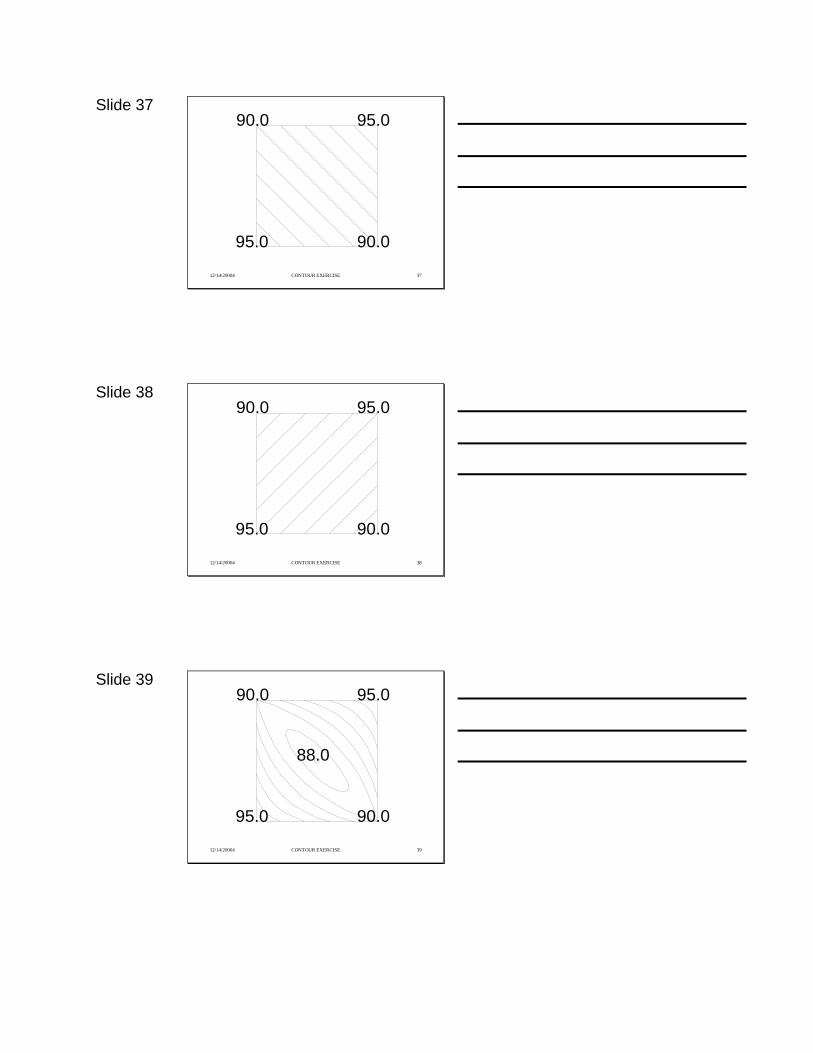
Slide 37
12/14/20004 CONTOUR EXERCISE 37
95.0
90.0
90.0
95.0
Slide 38
12/14/20004 CONTOUR EXERCISE 38
95.0
90.0
90.0
95.0
Slide 39
12/14/20004 CONTOUR EXERCISE 39
95.0
90.0
90.0
95.0
88.0
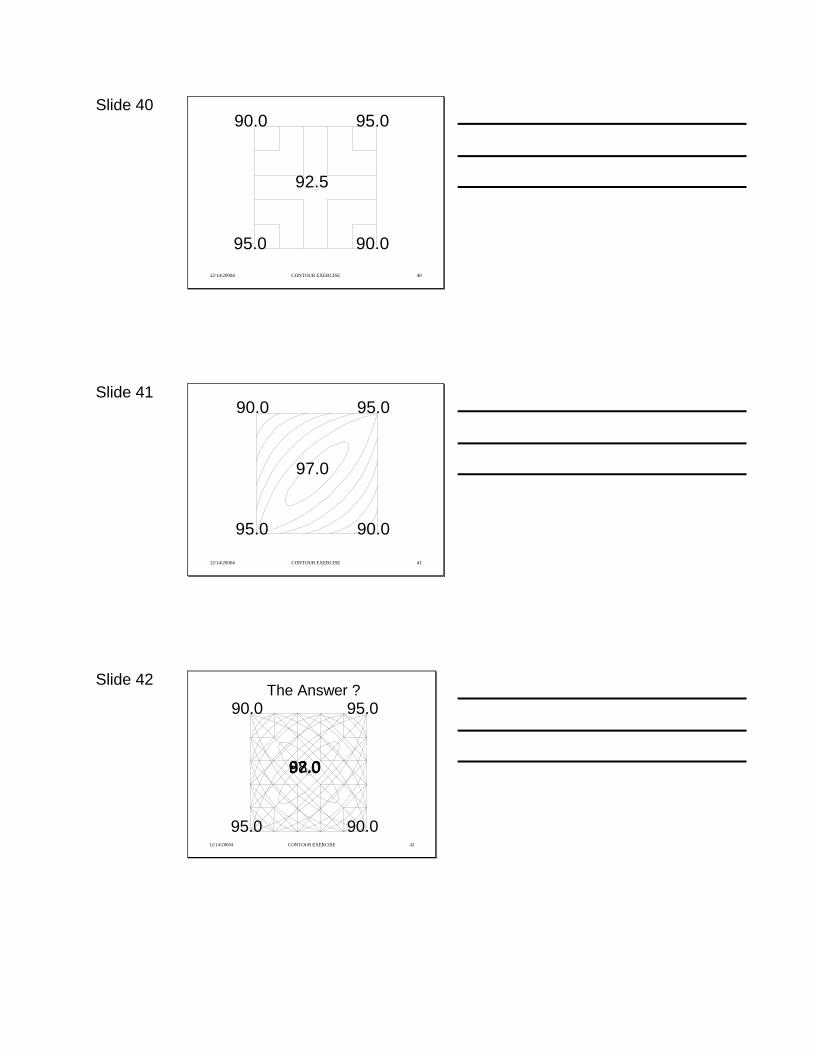
Slide 40
12/14/20004 CONTOUR EXERCISE 40
95.0
90.0
90.0
95.0
92.5
Slide 41
12/14/20004 CONTOUR EXERCISE 41
95.0
90.0
90.0
95.0
97.0
Slide 42
12/14/20004 CONTOUR EXERCISE 42
95.0
90.0
90.0
95.0
97.092.088.0
The Answer ?

Slide 43
12/14/20004 CONTOUR EXERCISE 43
Any one of the previous answers could be correct.
If you have seen the site you may be able to visualize what it should look like.
Otherwise you need additional readings.
The Right Answer

Tab for Profiles and Earthwork Info
Slide 1
01/12/03 PROFILES from Topo V2 1
PROFILESfrom a Topographic Map
Ohio Land ImprovementContractors Association
Ron Cornwell Paul DemuthFred & Rick Galehouse
Slide 2
01/12/03 PROFILES from Topo V2 2
OBJECTIVE
To use Elevations and Locations to display a Vertical Section
To display any problemsTo help design a construction plan
Slide 3
01/12/03 PROFILES from Topo V2 3
QUESTIONS
If you have questions along the way please ask them
There is a lot of information in this course and we will be proceeding rather quickly
There are no stupid questions

Slide 4
01/12/03 PROFILES from Topo V2 4
PROFILES
A profile is a vertical section through a proposed location.
A profile can be used to show the ground surface and also a proposed design
Slide 5
01/12/03 PROFILES from Topo V2 5
Profiles
Stations (STA) are a way of showing distance or locations on a plan or profile. Stations are commonly labeled something like 1+25 which would indicate 1 hundred and 25 feet
Slide 6
01/12/03 PROFILES from Topo V2 6
ProfilesOpen ditches and septic systems are
usually stationed from the top down Sub surface drains are usually stationed
from the outlet up
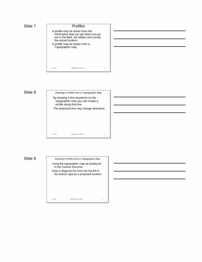
Slide 7
01/12/03 PROFILES from Topo V2 7
ProfilesA profile may be drawn from the
information that you get when you go out in the field, set stakes and survey the actual location.
A profile may be drawn from a Topographic map.
Slide 8
01/12/03 PROFILES from Topo V2 8
Drawing a Profile from a Topographic Map
By drawing a line anywhere on the topographic map you can create a profile along that line
The proposed line may change directions
Slide 9
01/12/03 PROFILES from Topo V2 9
Drawing a Profile from a Topographic Map
Using the topographic map we produced in the Contour Exercise
Draw a diagonal line from the top left to the bottom right as a proposed location.
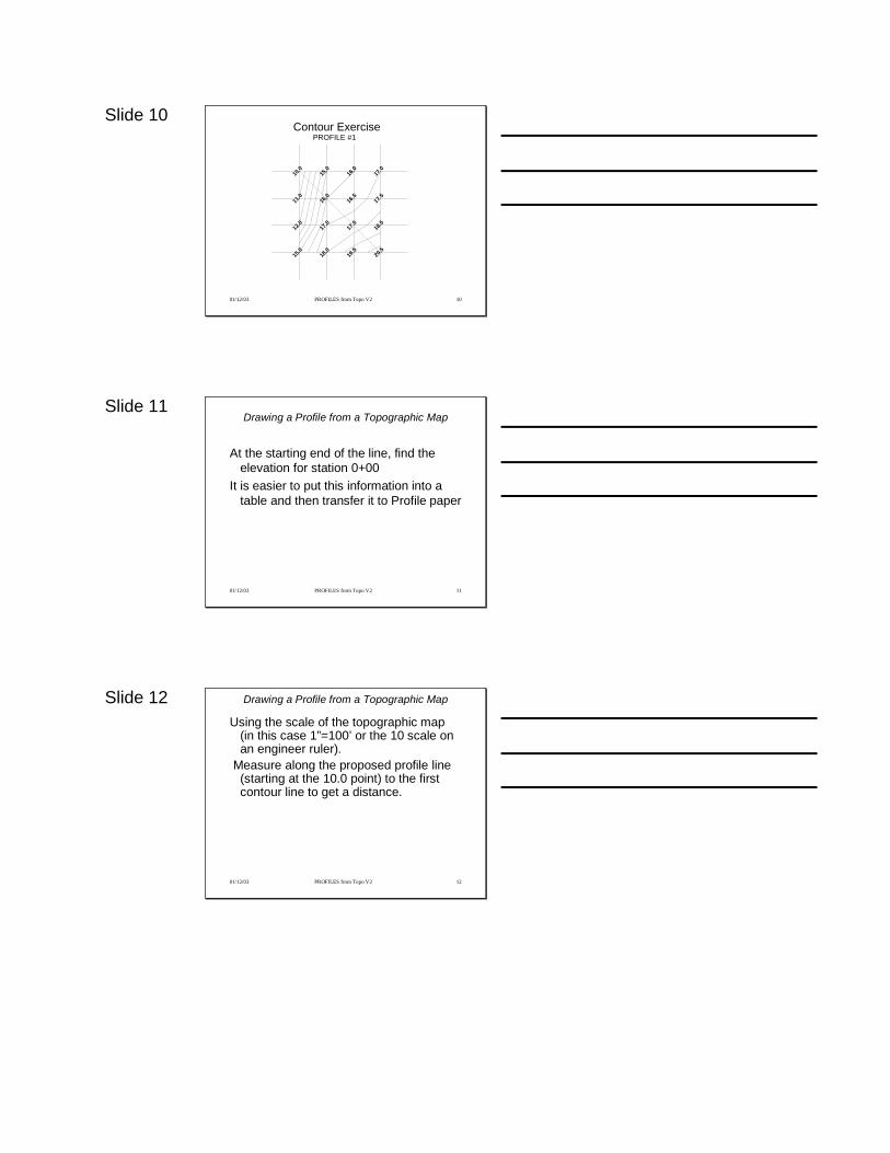
Slide 10
01/12/03 PROFILES from Topo V2 10
PROFILE #1Contour Exercise
11.0
16.0
15.0
12.0
18.0
17.0
10.0
15.0
16.5
17.5
20.5
18.5
19.5
17.5
17.0
16.0
Slide 11
01/12/03 PROFILES from Topo V2 11
Drawing a Profile from a Topographic Map
At the starting end of the line, find the elevation for station 0+00
It is easier to put this information into a table and then transfer it to Profile paper
Slide 12
01/12/03 PROFILES from Topo V2 12
Drawing a Profile from a Topographic Map
Using the scale of the topographic map (in this case 1”=100’ or the 10 scale on an engineer ruler).
Measure along the proposed profile line (starting at the 10.0 point) to the first contour line to get a distance.
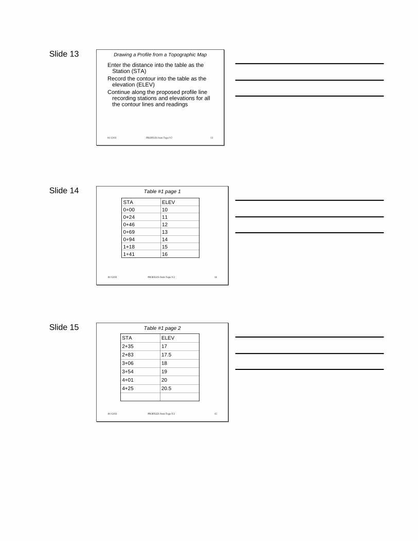
Slide 13
01/12/03 PROFILES from Topo V2 13
Drawing a Profile from a Topographic Map
Enter the distance into the table as the Station (STA)
Record the contour into the table as the elevation (ELEV)
Continue along the proposed profile line recording stations and elevations for all the contour lines and readings
Slide 14
01/12/03 PROFILES from Topo V2 14
Table #1 page 1
161+41151+18140+94130+69120+46110+24100+00ELEVSTA
Slide 15
01/12/03 PROFILES from Topo V2 15
Table #1 page 2
20.54+25
204+01193+54183+06
17.5 2+83172+35ELEVSTA
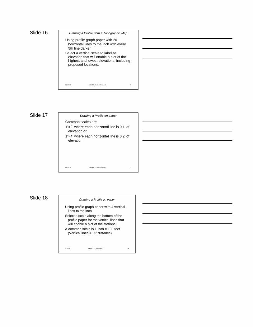
Slide 16
01/12/03 PROFILES from Topo V2 16
Drawing a Profile from a Topographic Map
Using profile graph paper with 20 horizontal lines to the inch with every 5th line darker
Select a vertical scale to label as elevation that will enable a plot of the highest and lowest elevations, including proposed locations.
Slide 17
01/12/03 PROFILES from Topo V2 17
Drawing a Profile on paper
Common scales are 1”=2’ where each horizontal line is 0.1’ of
elevation or 1”=4’ where each horizontal line is 0.2’ of
elevation
Slide 18
01/12/03 PROFILES from Topo V2 18
Drawing a Profile on paper
Using profile graph paper with 4 vertical lines to the inch
Select a scale along the bottom of the profile paper for the vertical lines that will enable a plot of the stations
A common scale is 1 inch = 100 feet (Vertical lines = 25’ distance)
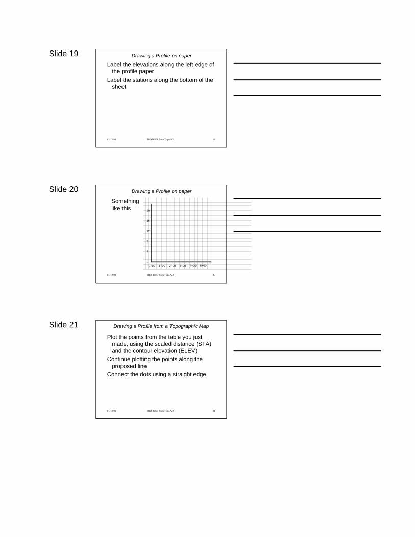
Slide 19
01/12/03 PROFILES from Topo V2 19
Drawing a Profile on paper
Label the elevations along the left edge of the profile paper
Label the stations along the bottom of the sheet
Slide 20
01/12/03 PROFILES from Topo V2 20
Drawing a Profile on paper
0
4
8
12
16
20
0+00 1+00 2+00 3+00 4+00 5+00
Something like this
Slide 21
01/12/03 PROFILES from Topo V2 21
Drawing a Profile from a Topographic Map
Plot the points from the table you just made, using the scaled distance (STA) and the contour elevation (ELEV)
Continue plotting the points along the proposed line
Connect the dots using a straight edge
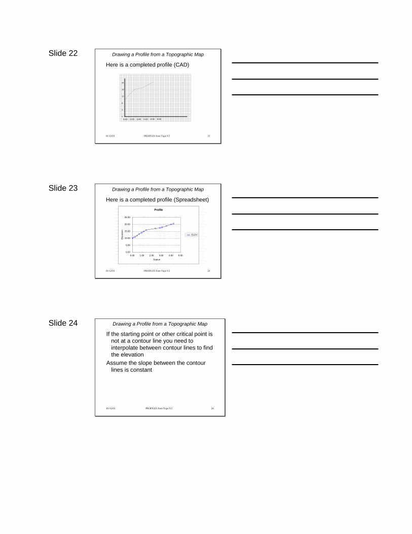
Slide 22
01/12/03 PROFILES from Topo V2 22
Drawing a Profile from a Topographic Map
Here is a completed profile (CAD)
0
4
8
12
16
20
0+00 1+00 2+00 3+00 4+00 5+00
Slide 23
01/12/03 PROFILES from Topo V2 23
Drawing a Profile from a Topographic Map
Here is a completed profile (Spreadsheet)Profile
0.00
5.00
10.00
15.00
20.00
25.00
0.00 1.00 2.00 3.00 4.00 5.00
Station
Elev
atio
n
ELEV
Slide 24
01/12/03 PROFILES from Topo V2 24
Drawing a Profile from a Topographic Map
If the starting point or other critical point is not at a contour line you need to interpolate between contour lines to find the elevation
Assume the slope between the contour lines is constant
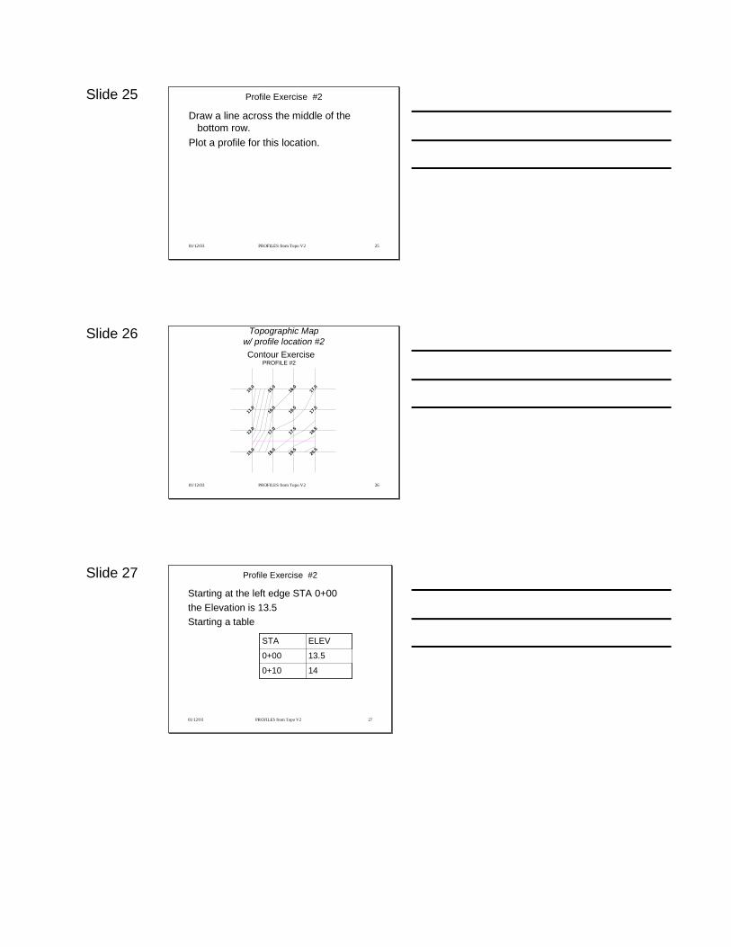
Slide 25
01/12/03 PROFILES from Topo V2 25
Profile Exercise #2
Draw a line across the middle of the bottom row.
Plot a profile for this location.
Slide 26
01/12/03 PROFILES from Topo V2 26
Topographic Mapw/ profile location #2
PROFILE #2Contour Exercise
11.0
16.0
15.0
12.0
18.0
17.0
10.0
15.0
16.5
17.5
20.5
18.5
19.5
17.5
17.0
16.0
Slide 27
01/12/03 PROFILES from Topo V2 27
Profile Exercise #2
Starting at the left edge STA 0+00the Elevation is 13.5Starting a table
140+10
13.50+00
ELEVSTA
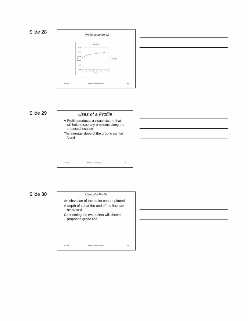
Slide 28
01/12/03 PROFILES from Topo V2 28
Profile location #2
Profile #2
0.00
5.00
10.00
15.00
20.00
25.00
0.00 0.50 1.00 1.50 2.00 2.50 3.00 3.50
Station
Ele
vatio
n
ELEV
Slide 29
01/12/03 PROFILES from Topo V2 29
Uses of a ProfileA Profile produces a visual picture that
will help to see any problems along the proposed location
The average slope of the ground can be found
Slide 30
01/12/03 PROFILES from Topo V2 30
Uses of a Profile
An elevation of the outlet can be plottedA depth of cut at the end of the line can
be plottedConnecting the two points will show a
proposed grade line
Slide 31
01/12/03 PROFILES from Topo V2 31
Uses of a Profile
The slope of the proposed line can be calculated
Cuts along the proposed line can be determined
Slide 32
01/12/03 PROFILES from Topo V2 32
Profiles
A profile may be drawn from a profile survey or a Topographic map
Surveyors with total stations can be hired to produce topographic maps
GPS systems can be used to help produce topographic maps
Slide 33
01/12/03 PROFILES from Topo V2 33
Uses of a Profile
Each Station can be checked for acceptable cuts.
An adjustment can be plotted and checked again.

Slide 34
01/12/03 PROFILES from Topo V2 34
Other ways to draw a profile
Computer spread sheet programs can draw profiles
Information is entered in the same way as in the field book
The formulas for figuring the distance and the elevations are entered and saved to be used again and again
Slide 35
01/12/03 PROFILES from Topo V2 35
Profiles from Topo
Are there any questions?
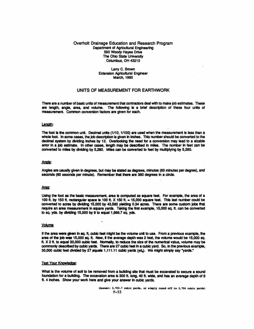
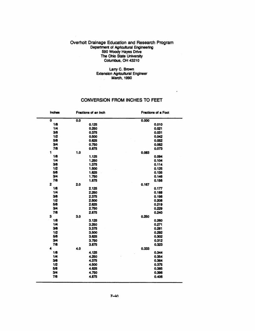
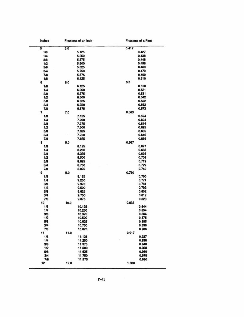
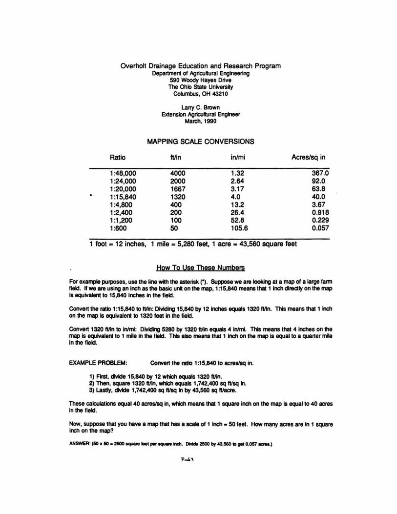

Tab for GPS and Mapping
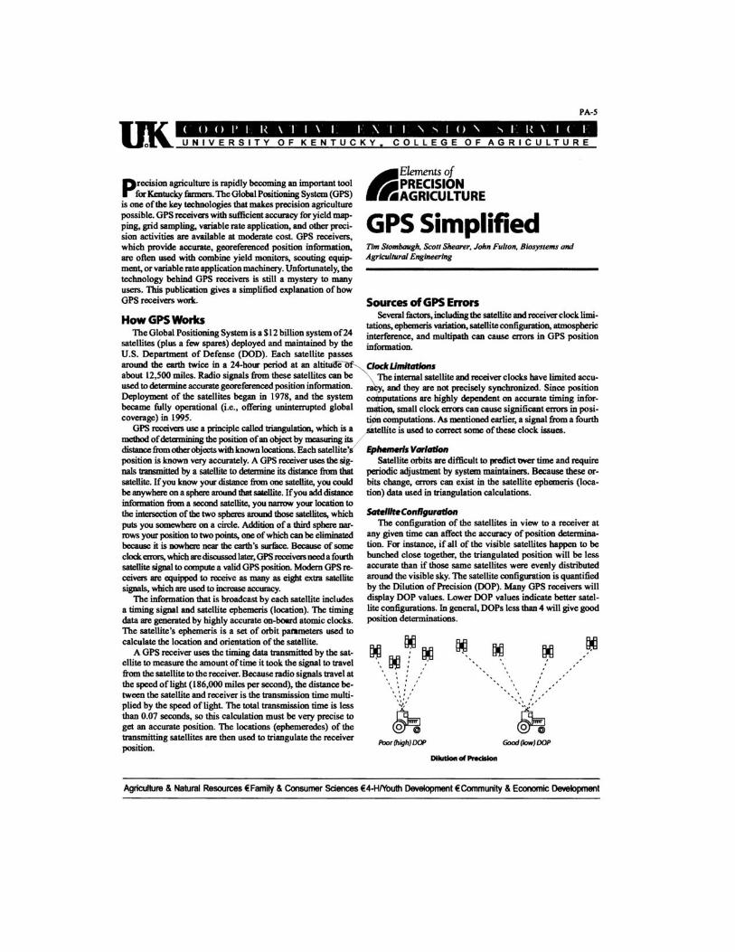
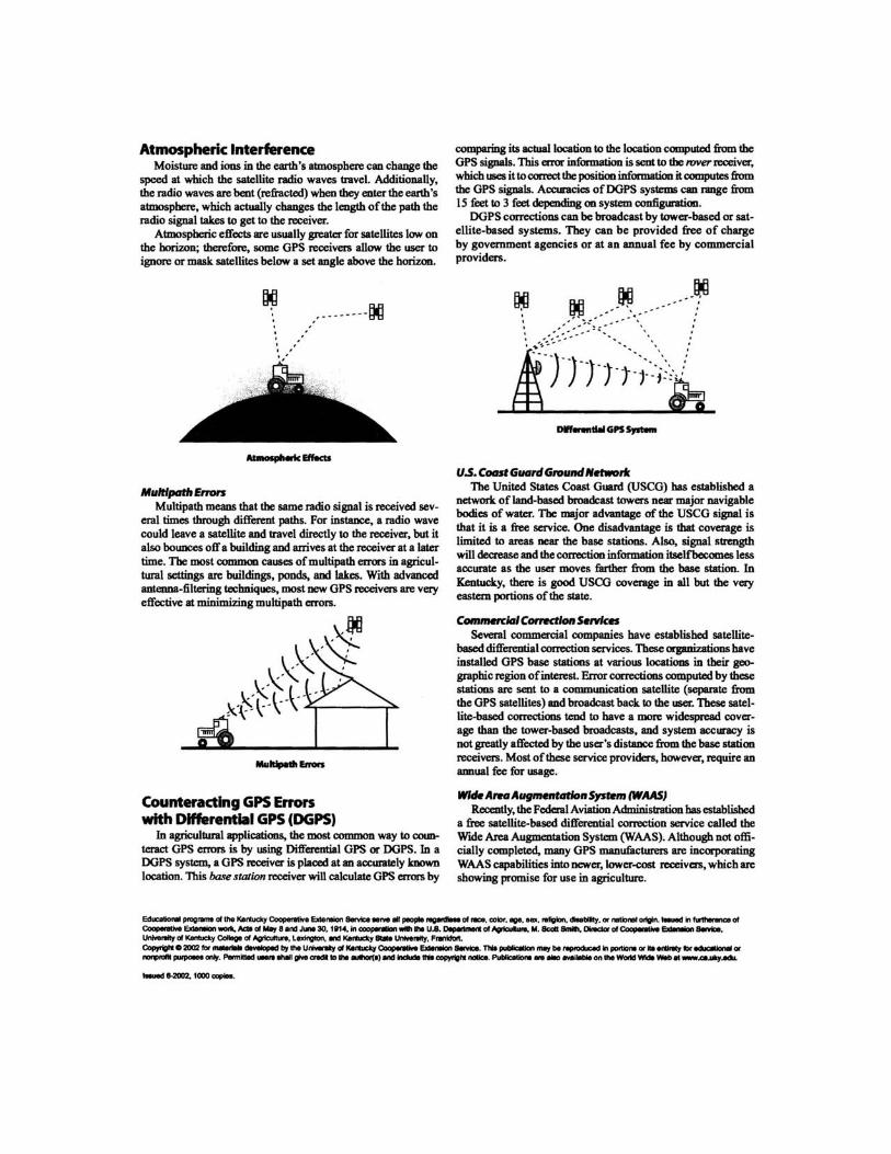
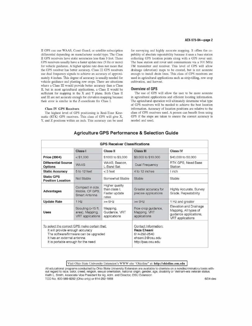

tab for Handout Materials