האוניברסיטה העברית בירושליםThe Hebrew University of Jerusalem

Faculty of Science

Fredy and Nadine Herrmann Institute of Earth Sciences

Ring Department of Atmospheric Sciences

Laboratory experiments and a consistent

theory for low-frequency waves over a

linearly sloping bottom on the f-plane

M.Sc. Thesis

Submitted by:

Yair Cohen ID 03645997

Thesis Advisor: Prof. Nathan Paldor

February 2009

Abstract: Low frequency waves that evolve in a fluid over a linearly slopping bottom on the

f–plane are investigated in two cases: An infinitely wide channel, with two long shore

boundaries and a shelf of finite width, where the fluid surface intersects the slopping

bottom at the shallow side while a long-shore boundary is present on the shelf's deep.

A Linear Shallow Water Model is solved for each of the two cases and the theoretical

results are compared to experimental findings.

In both cases numerical solutions reveal the existence of waves that propagate

with the shallow boundary on the right in the northern hemisphere. In a channel the

dispersion relation shows vanishing frequencies for both large and small

wavenumbers and a maximal frequency at a finite wavenumber. The frequencies were

found to differ from the classical harmonic theory by more than an order of unity in

wide channels or in steep slopes. In a shelf the dispersion relation shows vanishing

frequencies for small wavenumbers and a non-vanishing frequency that approaches a

constant value at large wavenumbers. These solutions are consistent with existing

asymptotic approximated solutions that were derived for an infinite shelf.

Both cases were tested in laboratory experiments on a 13 m diameter turntable at

LEGI-Coriolis (France). The linear slope in the experiments was 10% and the wave's

period and wavenumber were measured using a Particle Imaging Velocimetry (PIV)

technique. The experimental results regarding the dispersion relation and the radial

structure of the radial velocity are in good agreement with the (numerically derived)

theoretical predictions. These results clearly showed that in wide channels the

amplitude is trapped near the shallow wall.

In a channel a simple formula for the dispersion relation is developed by

approximating the velocity eigenfunctions by Airy function, which agrees with the

numerical solution for a wide channels or a steeply sloping bottom. These solutions

(that apply for infinitely wide channels as well) mandate that the waves occupy a

small part of the channel located close to the shallow side and vanish throughout most

of the channel width, so the channel width is filtered out of the problem provided it is

sufficiently large. A length scale for the channel’s width is found that defines the

harmonic regime and the Airy solution regime depending on the channels slope, wave

mode and wavenumber.

ii

Contents: Acknowledgments…………………………………………………. List of symbols……………………………………………………... List of figures……………………………………………………….

1. Introduction and background 1.1 General…………………………...…………………………. 1.2 The description of the problem……………………………... 1.3 Observational background……………………....................... 1.4 Theoretical Background………………………………….…..

A. Channel…………..………………………………………. B. Shelf………………..………………………......................

1.5 Experimental Background…………………………………... 2. Theoretical research

2.1 Formulation of the problem…………………………………. 2.2 The channel…………………………………………….…….

A. Exact - numerical results…………………..………….….. B. The harmonic limit…………………………………..…… C. Airy function solution……………………….……………

2.3 The shelf…………………………………………………….. A. Boundary conditions……………………………………... B. Local behavior and numerical solutions…….………...

3. Laboratory experiments 3.1 General………………………………………………………. 3.2 Physical setup and course of experiments………….………...

A. The tank…………...……………………………………… B. Wave generation technique………………..…….………... C. Wave imaging…………………………..…….…………...

3.2 Images analysis………………………………….…………… A. Velocity vector field…………………..…….……………. B. Period verification………………………...………………. C. Phase and amplitude……………………………..………..

3.3 Experimental Results………………………………………… A. Channel………...…………………………………………. B. Shelf………………...……………………………………..

4. Summery and discussion Bibliography……………….………..……………………………...... Appendix A…………………………...……………………………… Appendix B……………………………...……………………………

1 2 3 4 4 4 6 7 7 8 9 11 11 13 13 14 16 21 21 22 26 26 26 26 27 28 28 29 30 30 32 32 35 37 39 41 43

iii

Acknowledgments: My personal appreciation is given To my supportive parents To my supervisor Professor Nathan Paldor for the unique combination of guidance teaching and constructive criticism that led me to the presentation of this work To my friends at the GFD Laboratory - Ori Adam, Yair De-Leon and Andrey Sigalov for numerous contributing conversations and good company This work involves laboratory experiments that were taken at LEGI-Coriolis France I'd like to thank Hydralab-III 6th frame-work program for the funding of the experiments Professor Joel Sommeria, Mr. Henri Didelle and Mr. Samuel Viboud from LEGI-Coriolis laboratory for their guidance and the technical support in this part of the research

List of symbols: ( * - indicates dimensional parameters)

Variable Description

x long-shore horizontal Cartesian coordinate

y off-shore horizontal Cartesian coordinate

z vertical Cartesian coordinate

t time

H0 undisturbed depth at y=0 (dimensional constant)

H' the bottom slope (constant)

H the undisturbed depth (a function of y only: H=H0+H'y)

L channel width (in the off-shore direction)

f Coriolis parameter

Rd Rossby radius of deformation (Rd=(gH0)1/2/f )

u long-shore velocity

v off-shore velocity

η vertical displacement of the free surface from the mean height

k long-shore wavenumber

c long-shore phase speed

ω angular frequency

T period

δ non-dimensional parameter of the LSWE: *0H Rd Hδ ′=

2

List of figures:

1. Cross sections of the setups in the two different cases.

2. Numerical results showing dispersion relation and amplitude of TRW.

3. A comparison between numerically calculated TRW and the harmonic

approximation of TRW.

4. Solution of the Airy function.

5. Numerically calculated dispersion relation of first mode TRW in different

channel width compared with the Airy solution.

6. A comparison of dispersion relations obtained from numerical solution,

harmonic approximation and the Airy-function approximation.

7. Numerically calculated amplitudes of vertical displacement and off-shore

velocity of TRW in a channel for the first three modes.

8. Numerically calculated dispersion relation of continental shelf waves

9. Numerically calculated dispersion relation of the first quasi-geostrophic mode

continental shelf waves.

10. A radial cross section and a horizontal upper view of the tank.

11. Experimentally measured horizontal velocity vector field.

12. Experimentally measured time series showing the off shore velocity vs. frame

numbers.

13. Phase diagram and its tangential slice.

14. A comparison between numerical and experimental results for the dispersion

relation of TRW in two different channels.

15. Numerical and experimental radial amplitudes (eigenfunctions) of the off-

shore velocity.

16. A comparison between numerical and experimental results for the dispersion

relation of CSW.

3

Chapter 1

Introduction and background 1.1 General:

The Linearized Shallow Water Equation (hereafter 'LSWE') when applied for

a sloping bottom f-plane exhibits low frequency wave solutions (often referred to

as second class oscillations) that are analogous to the planetary Rossby waves

where the depth variations play the roll of Coriolis force variations in the strict

potential-vorticity considerations. These barotropic waves, whose frequency is

lower than the Coriolis parameter, are divided into two cases by the different

setups. One setup, referred as the 'channel', has two physical long-shore

boundaries and its low frequency waves are known as Topographic Rossby Waves

(hereafter 'TRW'). In the other setup, referred as the 'shelf', the sloping bottom

meets the free surface of the water at the shallow side and a long-shore physical

boundary is present only at the deep side. The waves that exist in this setup are

termed 'Edge Waves' and their low frequency class is known as Continental Shelf

Waves (hereafter 'CSW').

The topographic effect on fluid flow in meso-scale dynamics is of great

importance both in the ocean and in the atmosphere. It is analogues to Earth

curvature effect that mandates complicated flows patterns different from purely

uniform rotation flow in the synoptic scale. In specific, low frequency waves that

are a direct application of angular momentum conservation are governed by the

combination of rotation and depth variation forced by topography. This study

reports both theoretical and experimental investigation of these second class

oscillations in the two cases: First, for TRW in an infinitely wide channel where

the classical theory does not apply and second, for CSW on a finite shelf.

1.2 The description of the problem: This study includes an investigation of two different setups, see fig. 1 below.

In both setups are considered unbounded in the x-direction (long shore) and

bounded in the y-direction (off shore) and the bottom slope is a function of y only

and occupies the full width (i.e. off shore extant). The rotation is counter

4

clockwise as in the northern hemisphere and the Coriolis parameter is assumed

constant (hence planetary Rossby waves are excluded from this analysis).

The depth scale H0 is defined as the depth at y=0 and is assumed much smaller

than the vertical extant of the fluid. A more conventional definition of the depth

scale as the depth at the center of the channel is impractical when the channel

width is taken to infinity. The fluid is considered barotropic and the perturbation

from the state of motionless fluid and mean height of the free surface (z=0) is

described by a linear wave solution. In the channel (LHS in figure 1) with the two

long shore boundaries, solution are presented with the deep side wall taken

infinitely far on the positive y-direction. In the shelf case (RHS of figure 1) the

undisturbed depth vanishes at the shallow side (at y*=-H0/H') and a physical

boundary is found in the deep side only, solutions are presented for finite width

shelves.

H*0

y*

z*

H*0

x* L *

z*=0

η*

f

H*=0 y*=0

z*=0

H0/H'+ L*

η*

y*=L*

Figure 1: Cross sections of the setups in the two different cases. Both cases relate to the same

(right hand Cartesian) coordinate system and rotation as shown on the far left. On the left side, the

channel, with two long shore boundaries and width (L*) that is taken to infinity. On the right the

‘shelf’ of finite width where the undisturbed depth (H*) vanishes as the free surface interacts with

the sloping bottom and a long shore boundary at the deep side only. In the former y* is defined

from the vanishing point of the undisturbed depth to the deep side wall (i.e. -H0/H'<y*<L*).

5

1.3 Observational background: The difference between a flat bottom flow and a slopping bottom flow in the

meso-scale (i.e. on the f-plane) was first observed by Hamon (1962). Hamon

analyzed daily sea surface height data measured by tide gauges on the east

Australian coastline (Sydney and Coff's Harbor) and in the deep sea (Lord Howe's

Island). The analysis revealed a low frequency, non hydrostatic, northward

propagating anomaly in sea surface height that appeared unique to the continental

slope (i.e. a wave traveling with the coastline on the left hand side in the southern

hemisphere). Repeating analysis from tide gauges records confirmed these results

in different locations of the world: Hamon (1966) in the west Australia coastline,

Mysak and Hamon, (1969) in the coast of north Carolina and Mooers and Smith

(1968) in the coast of Oregon (these waves are found to travel with the coast on

the right in the northern hemisphere).

The St. Kilda (Scotland) sea level and current records showed a tidal slot that

occupies long period oscillations (in the order of 10 days) that were found

consistent with the frequency peaks of continental shelf wave theory (Cartwright,

1969). The analysis of sea level data from tide gauges and currents record (from a

vertical set of three current meters) near the coast of Oregon showed high

agreement with dispersion relations given from numerical model (Cutchin and

Smith, 1973). The observed phase between the off shore velocity and the free

surface variation showed some consistency with those predicted by the numerical

model.

The observational research exists mainly in oceanography even though these

wave solutions apply in the atmosphere as well. The theoretical terminology of

shelf waves and channel waves is equivocally used in some of the reported

observations yet, the observational research refers to the natural setup and the

attribution to any of the theories (shelf or channel) that is subjected to the physical

structure that mandates the choice of assumptions in every case, is left mostly for

theoreticians.

6

1.4 Theoretical Background: The horizontal motion of incompressible thin layer of fluid with a free surface

can be described by a set of partial differential equations know as the Shallow

Water Equations. These equations are the result of applying the hydrostatic

approximation on the pressure gradient in the horizontal components of Euler's

equation for a thin rotating layer of fluid along with the equation of continuity as

the connection between the vertical displacement and the horizontal velocity

divergence. When the amplitudes are small the non-linear components of the

equation are neglected and the resulting equations are known as the Linear

Shallow Water Equations (hereafter 'LSWE').

In barotropic wave theories these equations often supply enough simplification

of the full equations of motion in order to present analytical solutions (in apposed

to baroclinic waves, from example, where the equations of motion are more

complicated and further simplification is needed). The LSWE are therefore

considered preferable compared with other (more crude) assumptions, for example

zero horizontal divergence (see Caldwell et al., 1972 for comparison). Only such

LSWE based theoretical results are reviewed in following subsections.

A. Channel: Exact numerical solution for low frequency waves in a channel with an

exponential bottom slope, Caldwell et al. (1972), show dispersion curves with

vanishing frequencies for very small and very large wavenumbers and a non-

vanishing maximal frequency for finite wavenumber in all modes. These waves

propagate with the shallow wall on their right for northern hemisphere and their

off shore amplitude is found different than harmonic.

In a channel with a linearly sloping bottom the existing analytical solutions for

TRW are derived by assuming the coefficient in the governing equation as

constant thus harmonic solution can be presented (e.g. Cushman-Roisin, 1994 and

Pedlosky, 1986). In order for the coefficient in governing equation to be constant

the depth must be taken as constant. Yet these wave solutions are a direct result of

the depth variations and hence the depth variations must be kept (a specific

derivation of this approximation will be shown in section 2.2-B of this work).

This representation of the depth variation is analogues to the one used to

represent the Coriolis parameter variation in the classical solution for the planetary

Rossby wave. Yet, in the planetary case it is found that when the variations of the

Coriolis parameter are retained everywhere in the governing equation the

7

solutions can significantly differ from the one obtained in the classical planetary

theory and the amplitude of these waves shows clear non-harmonic behavior, i.e.

trapped waves (Paldor et al. 2007).

Furthermore, in this case the governing equation can be approximated as the

Airy function and thus non-harmonic analytical solutions are presented (Paldor

and Sigalov 2007). These new solutions show higher accuracy in the dispersion

relation (compared with numerical solutions) as well as a non-harmonic structure

of the amplitude. It is reasonable to assume that a similar analysis used in the

topographic case can provide new insights regarding the nature of TRW as well as

some new analytical approximations.

B. Shelf: The waves that form on a shelf with the vanishing of the undisturbed depth

at the shallow side (also known as beach conditions) are termed 'Edge waves'. It is

common to divide these waves into high frequency waves (first class) and low

frequency waves (second class, also termed CSW, as will be used hereafter) in this

research only this second class edge waves are investigated.

Solutions for second class edge waves on an infinite shelf with a linear bottom

slope (Reid, 1958) reveal waves that propagate with the shoreline on the right in

the northern hemisphere (as TRW) yet their group velocity (unlike the one of

TRW) do not change its sign. The first mode (termed fundamental mode) has

increasing frequencies with increasing wavenumber and as a result are much

larger than the Coriolis parameter as wavenumber increases. The frequencies of

the other modes (termed quasi-geostrophic modes) are associated with high

vorticity and show asymptotic convergence into finite values as the wavenumber

increases. These values that are always smaller than the Coriolis parameter are a

function of the wave mode and the Coriolis parameter only. Their group-velocities

as a result converge to zero for large wavenumbers (hence energy is transferred in

long waves only).

On a shelf with finite width with a linear bottom slope the solutions for (long

shore) wave length that is larger than the shelf width reveals waves that propagate

in the same manner as those found on the infinite shelf (Reid, 1958), yet are non-

dispersive and their frequency is a function of the shelf width (see Robinson,

1964, who termed them as CSW). These solutions, when compared with

observational record (Hamon, 1962), showed qualitative accuracy only. Numerical

solutions of the finite shelf (Mysak, 1968) show that as the wave length deceases

8

the solutions behave more like those of the infinite shelf, meaning for large

enough long-shore wavenumber (short enough waves) the solution are

independent of the shelf width.

1.5 Experimental background (channel only): To the best of my knowledge laboratory experiments of low frequency

topographic wave are presented in a channel only (i.e. TRW), until the writing of

this work no documented experiments on a shelf (i.e. CSW) was found. The

analogy between TRW and planetary Rossby waves as was pointed out in the

theoretical review has been an important part of the motivation for the early

laboratory experiments. While the experimental generation of planetary Rossby

wave is a highly complicated (if possible) challenge the generation of TRW in a

laboratory is a strait forward experiment that can demonstrate a qualitative

verification of the potential vorticity based phenomena (both the planetary and the

topographic). One of such experiment (reported by Platzman, 1968) was taken in a

38cm wide flat-bottom annulus (outer radius of 80cm) when the effect of rotation on

the free surface produced a parabolic depth profile. The generated was done by

moving a radial obstacle in a tangential direction with respect to the rotating

system and the waves that formed behind the bump in the downstream direction

showed good qualitative resemblance to theory.

Experiments that were oriented towards TRW were performed in more

quantitative methods in order to be compared with theories, yet all were

performed with a non-linear bottom slope. Phillips (1965) presented a verification

of theory with laboratory experiments in which similar technique for depth

variation (forced by rotational effect on the free surface) was used. These

experiments (see also Ibbetson, 1967 for a more detailed review) were performed

in a 30cm wide annulus (L/Rd=0.28) with a fixed rotation speed for which the

parabolic free surface would be tangent to the bottom at the rotation axis if the

inner boundary was removed (mid value of the slope was about 0.2 and f=0.75s-1).

The former constraint that connects the Coriolis parameter to the depth variation

simplified the equations in such manner to allow the presentation of analytical

solutions. The waves were generated by using radial barrier that was made to

oscillate about its central vertical axis. The wave length was measured by streak

photography of the annulus with aluminum flake inserted to the water as tracers

9

and the phase speed was determined by the observed propagation of the wave with

respect to the time difference between two frames. For very small and very large

wavenumber the analytical theory showed very high accuracy compared with the

experiments, yet for the maximal values of frequency (that is mid-values of

wavenumber) the experimental data showed values about 30% larger than those

showed by the theory.

Caldwell et al. (1972) presented a more advanced experimental setup in an

annulus where the depth variation (exponential) were obtained by an actual

bottom slope (a negative exponential slope) followed by a flat bottom part

analogues to a continental margin. This bottom was installed in an annulus with

parabolic shape so that the parabolic free surface of the water (formed due to the

high speed rotation) was parallel to the flat bottom part. Two different channel

widths were tested: (1) 16cm ‘wide-channel’ with depth at the shallow side 0.6cm

(L/Rd=4.1), (2) 8cm ‘thin-channel’ depth at the shallow side not mentioned

(L/Rd≈1.1) in both cases f=6.28s-1. The wave generation was made by a paddle

moving in a radial direction pushing water up and down the slope and the

measuring of waves was made with the use of aluminum tracers and streak

photography of the annulus similarly to former experiments. The experimental

dispersion relation were compared with numerical solutions and showed very

good agreement in both thin and wide channels. The radial distances of the

maximal amplitude in the numerical solutions were compared with the location of

minimal motion in the experimental images and found to be in good agreement.

10

Chapter 2

Theoretical research

2.1 Formulation of the problem: Since the difference between the two cases lays in the boundary condition at

the shallow side of the domain the formulation of the wave equations prior to the

use of boundary conditions (hereafter B.C.) is common. For small amplitude,

undamped wave solution in a thin uniform rotating layer of fluid the equations of

motion can be reduced to the LSWE. Here x* and y* are defined as the long shore

and off shore coordinates respectively, u* and v* are the long shore and off shore

velocity components respectively and η* is the horizontal displacement of the free

surface from the mean height. The depth is defined as H*=H0+H'y, where H'

(positive constant) is the derivative of H* with respect to y*.

In a right hand Cartesian coordinate system these equations in their

dimensional form are as follow: **

** *

0u fv gt x

η∂ ∂− + =

∂ ∂ (1.1)

**

* *0v fu g

t yη∂ ∂

+ + =∂ ∂

* (1.2)

* * **

* * *0u v H vH

t x yη ⎛ ⎞∂ ∂ ∂ ′++ +⎜ ⎟∂ ∂ ∂⎝ ⎠

= (1.3)

In order to minimize the number of parameters in the equation system it is

customary to non-dimensionalize the variables. The depth is scaled by H0 (the

depth at y=0), the time is scaled by f -1 and the horizontal length is scaled by the

radius of deformation ( 0Rd gH= f ). By this scaling the non-dimensional form

of equation system (1) is written with the use of a single non dimensional

parameter δ:

0u vt x

η∂ ∂− + =

∂ ∂ (2.1)

0v ut y

η∂ ∂+ + =

∂ ∂ (2.2)

( )1 u vyt x yη δ

⎛ ⎞∂ ∂ ∂+ + + + =⎜ ⎟∂ ∂ ∂⎝ ⎠

0vδ (2.3)

11

Here the non-dimensional depth is written as H=1+δy and the new non-

dimensional parameter: 10H RdHδ −′= includes the depth scale the length scale

and the sloping of the bottom. With this choice of scaling the velocity is scaled

by 0gH , the phase speed of Kelvin waves at the shallow wall, hence the

frequency of TRW (ω=ck) is expected to be smaller than the order of unity.

Limiting ourselves to waves that propagate parallel to the shore we farther assume

a wave like dependence on the long shore direction for all three function, i.e.

u,v,η~exp(i(kx-ωt)) here k is the wavenumber, c is the phase speed and ω is the

frequency (ω=ck). This enables us to represent the temporal derivative and long-

shore spatial derivative as the frequency and wavenumber respectively. By

defining a complex function 1V ik −= , a non-complex system is obtained:

0c u V η⋅ − − = (3.1)

2 0u k c Vyη∂

− ⋅ + =∂

(3.2)

( ) ( )1 1 Vy u y V cy

δ δ δ η∂− + + + + + =

∂0 (3.3)

Equation (3.1) presents a simple algebraic connection between u,V and η thus

equations (3.2) and (3.3) can be reduced to a couple of first-order differential

equation for η,V only, hereafter the η,V equations:

21 1V k cy cη η∂ ⎡ ⎤= − + −⎢∂ ⎣ ⎦c ⎥

(4.1)

1 11 1

V c Vy c y c

δηyδ δ

⎡ ⎤ ⎡ ⎤∂= − + −⎢ ⎥ ⎢∂ + +⎣ ⎦ ⎣ ⎦

⎥ (4.2)

The η,V equations are the starting point for the numerical solutions and the

analytical approximations both in the channel and the shelf cases. In the channel

solutions can be found for these equations directly. In the shelf case these equation

present both a non-simple boundary condition and a singular behavior in the

shallow side and therefore cannot be numerically integrated without determining

the local behavior of the two eigenfunctions near the singular point.

12

2.2 The channel: A. Exact - Numerical results: The η,V equations in a channel with two B.C. for V

provided by the two walls is a well defined system that can be numerically

integrated given a normalization value for η at one wall. Since the V,η equations

present derivatives with respect to y only they can be numerically integrated as a

system of ordinary differential equations (ODE). Here the integration is performed

by using the BVP4C package in MATLAB with V=0 at the two walls and η=0.1

and the shallow side wall. The BVP4C package solves ODE as a boundary value

problem in a finite-difference collocation method (up to fourth order accuracy)

that is subjected to both B.C. at all times.

Solution are presented both by the value of the phase speed (c) and by plotting

the eigenfunctions (η and V). Three, well known, wave types are found in the

results: the non dispersive Kelvin wave, the dispersive high-frequency Poincare

waves and the dispersive low-frequency TRW. The identification of the wave type

(i.e. Poincare, Kelvin or TRW) is done according to the value of c, as was

mentioned in section 2.1, and the mode is determined by the number of zero

crossings of V. Since this study focuses on TRW the higher frequency shallow

water wave type that were found will not be shown. Numerical results of TRW are

shown in figure 2.

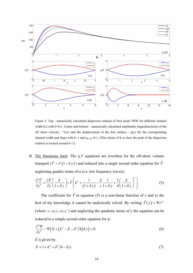
The dispersion relation for the indicated values (top panel of figure 2) clearly

shows that as L increases ω increases as well. Yet for L>10 ω is found to

converges to the same values (see the difference between the plots for L=10 (red)

and L=30 (blue) in the top panel). For L<10 the amplitudes of the eigenfunctions

are shown to be similar to harmonic with the maximal amplitude (and hence the

maximum of the energy) located in the center of the channel see the center left and

center right panels of figure 2. As L increases (L≥10) the amplitudes are shown to

be trapped against the shallow side wall with the location maximal amplitude

limited to y≈3 see figure 2, bottom right and left panels. These qualitative features

of the solutions are found consistent throw a verity of different values of δ and for

different wave modes and following these conclusions the different analytical

approximations for the V,η equations are examined.

13

0 1 2 3 4 5 60

0.01

0.02

0.03

0.04

0 0.5 1 1.5 2 2.5 3-5

0

5

0 2 4 6 8 10-5

0

5

y

0 5 10 15 20 25 30-5

0

5

0 1 2 3 4 5-5

0

5

ηV

ηV

ηV

ηV

L=3L=30L=10L=5

L=5

L=30

η,V

η,V η,V

y y

ω

L=3

L=10

y

δ=0.1

k

η,V

Figure 2: Top - numerically calculated dispersion relation of first mode TRW for different channel

width (L) with δ=0.1. Center and bottom – numerically calculated amplitudes (eigenfunctions) of the

off shore velocity - V(y) and the displacement of the free surface - η(y) for the corresponding

channel width and slope with k=1 and η(y=0)=0.1. (This choice of k is since the peak of the dispersion

relation is located around k=1).

B. The Harmonic limit: The η,V equations are rewritten for the off-shore volume

transport ( (1V V )yδ= + ) and reduced into a single second order equation for V

neglecting quadric terms of ω (i.e. low frequency waves):

( )

222

2

1 1 11 1 1 4 1

V V V ky y y c y yy

δ δδ δ δ

⎛ ⎞⎛ ⎞ ⎛ ⎞∂ ∂ ⎜ ⎟= + + − +⎜ ⎟ ⎜ ⎟⎜ ⎟∂ + + + +∂ ⎝ ⎠ ⎝ ⎠⎝ ⎠

δδ

(5)

The coefficient for V in equation (5) is a non-linear function of y and to the

best of my knowledge it cannot be analytically solved. By writing

(where

( ) ayV y e= Ψ

( ) 12 2a yδ δ −= + ) and neglecting the quadratic terms of y the equation can be

reduced to a simple second order equation for ψ:

( )(2

2 22 4E k E y

yδ δ∂ Ψ

−Ψ + − − =∂

) 0 (6)

E is given by: 2 21 4E k cδ δ= + + − (7)

14

Since the depth never vanishes in the channel a ≠−∞ the same vanishing

points (i.e. the same B.C.) apply for both ψ and . The elimination of quadric

terms in δy can be justified by the numerical results shown in figure 2, showing

that the eigenfunctions are limited to a small extant of the channel near the

shallow wall (i.e. near y=0).

V

The harmonic approximation of equation (6) can be obtained by eliminating

both δ2/4 and non constant term in the coefficient, resulting in a constant

coefficient equation. The general solution of this constant coefficient, governing

equation, is a linear combination of harmonic functions (sine and cosine). Given

the B.C. at the shallow wall the cosine function is rejected and given the B.C. at

deep side wall an equation for the phase speed is written, with the wave mode

(n+1) and channel width (L) introduced as parameters in the solution:

( )22 2 21 1k

k n L

δωπ

=+ + +

(8)

In order for the coefficient to be constant either δy must vanish or the

following condition must apply for the wavenumber: k2=δ2/2-(n+1)2π2/L2. In any

other wavenumber value only the vanishing of δy can yield this constant

coefficient approximation. In order for δy to vanish a very small slope and a very

narrow channel must be considered.

Equation (8) that is found in various text books (e.g. Pedlosky - 1982,

Cushman-Roisin – 1994) is the classical harmonic solutions for the dispersion

relation of TRW. Here n represents the number of nodal points (number of zero

crossing) of the velocity eigenfunction that is the wave's mode and it can be seen

that lower mode will have a higher phase speed. Figure 3 shows the dispersion

relation of TRW as calculated from equation (8) compared with the numerical

solution of the former section for various values of δ and L.

The sign of the phase speed resembles the sign of δ, hence for northern

hemisphere (f >0) these waves propagate in a long shore direction with the

shallow wall on the right hand side (and in with the shore on the LHS in the

southern hemisphere). It can be seen that for small δ and L (top left panel of figure

3) the harmonic approximation is good. When increasing δ (top right panel of

figure 3) the error increases, in this case about 60% of the numerical value. For

large values of both δ and L (both bottom panels) the error can increase up to the

order of 400% from the numerical value.

15

Equation (8) with the channel width taken to infinity for k=1 and n=1 the

dispersion relation tends to a value of 0.5.δ. For δ=2 this value approaches 1 (see

left bottom panel). As was shown earlier in figure 2, with increasing values of

channel width beyond 10 the numerically calculated dispersion relation is almost

unchanged hence the wide channel example bottom left panel of figure 3

approximately corresponds to the maximal error in this choice of δ.

0 1 2 3 4 5 60

0.01

0.02

0.03

0.04

0 1 2 3 4 5 60

0.05

0.1

0.15

0.2

0 1 2 3 4 5 60

0.2

0.4

0.6

0.8

1

0 1 2 3 4 5 60

0.1

0.2

0.3

0.4

0.5

HarmonicNumeric

HarmonicNumeric

HarmonicNumeric

HarmonicNumeric

k k

k

L=3δ=0.5

L=3δ=0.1

kL=5δ=1

L=20δ=2

ω

ωω

ω

Figure 3: A comparison between numerical solution (blue) and the harmonic approximation (red) for

the dispersion relation of first mode TRW for various values of δ and L as indicated in the RHS of

each panel.

The structure of the amplitude in the numerical solution is found to be similar

to harmonic for thin channels only, in wide channels the structure decays and

implies a non harmonic behavior of the eigenfunctions and hence the former

assumption that yielded a constant coefficient equation ( 0Lδ ≈ ) has a limited

level of accuracy and solution for the non constant coefficient equation, if exist,

might reveal different characters of the waves.

C. The Airy function solution: In the case of an infinitely wide channels harmonic

solutions which predicts that the waves must occupy the full width of the channel

(infinity in this case) are somewhat unaccountable. In this section a less crude

approximation for the coefficient in equation (6) will be presented in order to

derive non harmonic analytical solutions that might prevail in infinitely wide

channels. Since the coefficient in equation (6) is linear it is possible (following

16

Paldor and Sigalov, 2007) do define a new independent variable Z and to rewrite

equation (6) as: 2

2 ZZ

∂ Ψ= Ψ

∂ (9)

Here Z is defined as:

( ) ( ) ( )( )2 32 2 2 3 2 24 4Z y k E E k E yδ δ δ− −= − − + − − δ (10)

Equation (9) is the Airy function and its general solution is a linear

combination of two semi-harmonic functions Ai and Bi (see figure 4). Both

functions are oscillating on the negative part of Z axis while on the positive part Ai

is exponentially decaying and Bi is exponentially growing. The vanishing points

of Ai (marked as Zn) are an infinite set of irrational numbers and their asymptotic

approximation can be found in literature (Abramowitz and Stegun, 1972) the first

four shown in figure 4 are approximately Z0=-2.3811, Z1=-4.08795, Z2=-5.5205,

Z3=-6.7867.

-10 -8 -6 -4 -2 0 2 4 6

-0.4

-0.2

0

0.2

0.4

0.6

0.8

Z

Bi(z)

Ai(z)

Z0Z1Z2Z3

Figure 4: Solution of the Airy function. Both solutions are oscillating on the negative part of Z

axis. On the positive side Ai (in red) is decaying solution and Bi (in dashed blue) is growing. Since

only Ai is used in this study only the vanishing points of Ai are indicated.

When placing the shallow side wall of the channel at the nth vanishing point of

Ai (i.e. demanding Z=Zn when y=0) and the deep side wall far enough on the

positive of the Z axis, the contribution of Bi (the growing function) can be

neglected. Thus, analogues to the procedure made with harmonic functions in the

17

former section, here Bi is rejected by the B.C. and Ai alone is sufficient in order to

present an approximated solution. The far wall must lie at least at Z=4 in order to

allow the decaying of Ai to a negligible value (order of 10-8.Bi). By Neglecting E

with respect to k2 a simple formula for the phase speed for TRW is presented:

2 2 4 3 2 31 4 n

kk k Z

δωδ δ

=+ + +

(11)

Placing the nth vanishing point of Ai in equation (11) results in n zero crossing

point of the velocity function and represents the nth mode of the wave. From the

requirement of Ai<<Bi it is clear that a minimal channel width is necessary for the

applicability of this new solution, yet for any channel-width larger than this

threshold (even for an infinitely wide channel) the solution is the same. In the top

panel of figure 5 the numerical plots shown in section 2.2-A (figure 2 top panel

with δ=0.1) are compared with the Airy function solution for the infinitely wide

channel. It can be seen that as the channel width increase the numerical solution

are converging to the Airy solution. For L≥10 the difference is negligible. In the

bottom panel of figure 5 the same comparison is done for δ=2 it can be seen that

the maximal accuracy is less than the one obtained with δ=0.1, yet is still highly

accurate when compared with harmonic solution (see left bottom panel of figure 6

in this subsection).

0 1 2 3 4 5 60

0.01

0.02

0.03

0.04

L=3L=30L=10L=5Airy

0 1 2 3 4 5 60

0.1

0.2

0.3

0.4

L=3L=5L=10L=30Airy

k

δ=2

ω

ω

δ=0.1

Figure 5: Numerically calculated dispersion relation of first mode TRW in different channel

width (as indicated) and for two δ different values compared with the Airy function solution

(light green) for the corresponding slope values.

18

By placing equation (11) as the term for the phase speed in E the following

condition for E+δ2/4 to be negligible with respect to k2: k2»δ2/4-|Zn|k4/3δ2/3. In first

mode wave this condition apply k>0.01 when δ=0.1, for k>0.1 when δ=0.5, for

k>0.18 when δ=1 and k>0.35 when δ=2. Yet, this new formula for the dispersion

relation (equation 11), that is independent of the channel width, is equivalent to

taking the channel width to infinity and when compared with the expression that

result from the harmonic case for infinitely wide channel (i.e. equation 8

for ) it is much closer to the numerical values even in cases that do not

satisfy the above condition, see the bottom left panel of figure 6 with δ=2 and

wavenumbers smaller than the required value given by the above condition (in this

case 0.35).

L →∞

0 1 2 3 4 5 60

0.01

0.02

0.03

0.04

0.05

0 1 2 3 4 5 60

0.05

0.1

0.15

0.2

0 1 2 3 4 5 60

0.2

0.4

0.6

0.8

1

0 1 2 3 4 5 60

0.1

0.2

0.3

0.4

0.5

HarmonicNumericAiry

HarmonicNumericAiry

HarmonicNumericAiry

HarmonicNumericAiry

L=20δ=2

L=3δ=0.1

k k

ω ω

k

ω

L=5δ=1

k

L=3δ=0.5

ω

Figure 6: A comparison between numerical solution (blue) the harmonic approximation (red) and

the Airy-function approximation (green) of TRW for various values of δ and channel width.

Similarly for figure 3, with increasing channel width (L) the harmonic solutions increases the yet

the numerical solution is limited and the Airy function solution is independent of the channel's

width.

For first mode wave with k=1 and L taken to infinity, equation (11) tends to

the value of δ/(2+δ2/4+δ2/3|Zn|) and equation (8) in the harmonic case tends to a

value of δ/2. For small δ the difference is not large yet as δ increases the

difference increase significantly. For δ=1 the dispersion relation from equation

19

(11) is ω≈0.22, this value that is a good approximation for the numerical result

shown in the bottom right hand side of figure 6 (in blue) and is approximately a

half of the value that results from the harmonic theory (0.45). For δ=2 the solution

from equation (11) can be a less than third of the values given by the harmonic

theory (bottom left panel of figure 6).

Since the harmonic solution presented in equation (8) grows with increasing

channel width and the Airy function solution of equation (11) is invariant to

increasing channel width it is possible to find a critical channel width ( L ) for

which the two solutions converge. For channel width larger than L the harmonic

solution is larger in value and hence this equilibrium value is the minimal channel

width for which the Airy solution is a better approximation than the harmonic

solution. This threshold value, a function of the wave mode wavenumber and

slope, is given by:

( ) ( ) ( )1

2 4 3 2 21 4 nL y n Z kπ δ δ 3 −= + + (12)

0 2 4 6 8 10 12 14 16 18 20

-0.5

0

0.5

y

0 2 4 6 8 10 12 14 16 18 20-0.5

0

0.5

0 2 4 6 8 10 12 14 16 18 20-0.5

0

0.5

ηV

ηV

ηV

η, V

first mode

second mode

third mode

Figure 7: Numerically calculated vertical displacement (blue) and off-shore velocity (red)

amplitudes of TRW in a channel for the first three modes, L=20, k=1 and δ=0.5. The value of η at

the shallow side wall (y=0) is normalized as 0.1 at the first and third mode yet at -0.1 at the second

mode in order to present sign coherence in all profiles.

20

Since this value is a function of the wavenumber for any finite channel-width

there exist a small enough value of wavenumber for which the harmonic

approximation is better, for any larger value of wavenumber the Airy solution

prevails. The amplitude of the Airy-function solution (Ai) decays on the positive

side of Z, for all modes, faster than exponential decay. Hence the former analysis

mandates that: For a given wave mode, far enough from the shallow wall there

are no TRW in spit the presence of a sloping bottom! The energy (most of which is

in the lower modes) is trapped near the shallow wall. This character agrees well

with the numerically calculated amplitude presented for the first three modes, see

figure 7.

2.3 The shelf: In this section numerical solutions are presented in a similar manner as in the

former section and compared with asymptotic approximation for the infinite shelf

(Reid, 1958). The absence of a shallow wall implies that the depth scale is a

function of the slope (i.e. H0=(H')-1) and hence the slope and the channel width are

the only parameters that defines the physical setup (no depth scale exists in the

system). Since the long shore wave length must be measured by the channel width

it is expected that increasing the shelf width will be equivalent to increasing the

long shore wavenumber (k). By this it is clear that in any shelf width some

wavelength will be small enough in order for the shelf to be effectively infinite

(see figure 1 in Mysak, 1968).

A. Boundary conditions: The boundary conditions in the shelf present two obstacles

for the numerical integration of the η,V equations. First: in the absence of a wall at

the shallow side, demanding regularity on V at the shore line is the alternative

B.C. (e.g. LeBlond and Mysak 1978). Yet the η,V equations show irregular

behavior at that point dew to the vanishing of the undisturbed depth (i.e. placing

y=-δ-1 in equation 4.2). Second: at the shoreline the connection between V and η is

given as a function of the phase speed thus further complicating the numerical

integration. It was found best to define 1h yδ= + as the new independent

variable and rewrite the η,V equations for two new functions , 2V Vh= c hη η=

thus a new equation system is obtained:

21

2 2 1 1 22 k c hVh hη η

cδ δ⎡ ⎤∂ − ⎛= + ⎜⎢ ⎥∂ ⎝ ⎠⎣ ⎦

⎞− ⎟ (13.1)

2

2

2 2V h hVh c c

η 2δ δδ

⎡ ⎤∂= + −⎢∂ ⎣ ⎦

⎥ (13.2)

Here V is same function used in section 2.2-B and 2.2-C. In equation system

(13) both functions vanish at the shoreline dew to the vanishing of the undisturbed

depth and V vanish at the deep side wall dew to vanishing of V. The connection

between the two functions at the shoreline is independent of the phase speed. Yet

at the shoreline h vanishes as well and since one of the coefficients of η in

equation (13.1) is in the order of h-1 the behavior of the eigenfunctions at the

shoreline is not well defined.

B. Local behavior and numerical solutions: In order to numerically integrate equation

system (13) the behavior of both functions near of the shoreline must be analyzed.

By writing the functions as a two different power series expansions for h (i.e.

0 ,V V h h0α βη η∼ ∼ ) equation system (13) can be written as an indicial equation

system: 2 2

10 0 0

12 k ch V h hc

β α ββη η ηδ δ

− −⎡ ⎤−= + −⎢ ⎥⎣ ⎦

1 10

2 hβ + (14.1)

1 1 20 0 02

2 2 2V h V h h hc c 0

α α βα ηδ δ

βηδ

− + += + − (14.2)

For infinitesimally small values of h (i.e. h«1) components with higher order

of h are neglected and the simplified equation system presents two allowed

relations between α and β: (1) Equation (14.1) yields the condition β-1=α yet

when placed in equation (14.2) yields a trivial solution (α=0, β=1). (2) Equation

(14.2) yields the condition α-1=β, when placed equation (14.1) yields a non trivial

solution (α=2, β=1). Since in the former (non-trivial) solution both α and β are

larger than unity the behavior at the shoreline is regular. The indicial equation

(14.1) with the values of α and β given from (14.2) reveals the local behavior of

the two eigenfunctions near shoreline with the following relation:

( ) ( )11V h hδ η−= − 1 , see Bender and Orszag (1978) for a detailed review of this

technique.

Following this, equation system (13) can be numerically integrated in the same

technique used in the channel (given a normalization value for η near the

shoreline) yet here it is done from an infinitesimally small step from shoreline to

22

the deep side wall thus avoiding the singular point at the shoreline. The B.C.

applied for V are the local behavior near the shoreline normalized by the given

values of η and the vanishing at the deep side wall.

The numerical integration of equation system (13) shows two types of low

frequency waves that exist on the shelf both propagating with the shore on the

right (see figure 9 below). (1) A first mode wave with zero nodal points (black

line in figure 9) and frequency that is smaller than the Coriolis parameter for small

wavenumbers only yet increases and has non vanishing group velocity for large

value of wavenumber. (2) All other wave modes, with one or more nodal points

(red lines in figure 9) and frequencies converging to finite values (and vanishing

group velocities) as wavenumber increases. The second type that shows low

frequencies for all wavenumbers and is associated with high vorticity (Reid 1958)

is investigated here both numerically and experimentally.

0 2 4 6 8 10 12 14 16 18 200

0.5

1

1.5

2

2.5

3

X: 20Y: 0.324

X: 15Y: 0.195

k

n=0

n=1

ω

n=2

Figure 9: Numerically calculated dispersion relations of the first three modes of CSW, L=1, δ=0.5.

The fundamental mode (n=0) in black shows non decaying group velocity for large values of k

while the next two quasi-geostrophic modes shown here in red (n>0) have vanishing group

velocities for large values of k. The two data points presented on the n=1 and n=2 plots show the

value for which the frequency converges (indicated as Y axis values).

23

The dispersion relation of these waves is asymptotically approximated by Reid

(1958), these approximations rewritten for the scaling by which equation system

(4) is derived are as follows:

For large wavenumbers (k»δ)

12 1n

ω =+

(15)

For small wavenumbers (k«δ)

kω δ= (16)

Both equations (15) and (16) are approximations for infinite shelf yet they

show very high accuracy compared with the numerical solutions for a finite shelf

(see the indicated values in figure 9). For small wavenumbers the slope of ω as a

function of k (i.e. the group velocity) is given simply by δ. This value is consistent

with the numerical prediction as shown in the top panel of figure 10 (see the

dashed black line compared with the numerical solutions). It is found that as the

shelf width increases this asymptotic value given by equations (15) is found

consistent throughout larger values of wavenumbers as can be expected since the

shelf width is the only length scale and increasing it is equivalent to decreasing the

wavenumber.

0 5 10 15 20 25 30 35 400

0.1

0.2

0.3

0.4

δ=0.8δ=0.5δ=0.1

0 1 2 3 4 5 6 7 8 9 100

0.1

0.2

0.3

L=10L=5L=1

ω

k

ω

δ=0.5

L=1

Figure 10: Numerically calculated dispersion relation of the first quasi-geostrophic mode CSW on

a shelf for various values of non dimensional shelf width (top) and for various values of δ

(Bottom). The black dashed line in the upper panel indicates the asymptotically derived value for

small wavenumbers in the infinite shelf (Reid 1958) given in equation (16).

24

In the bottom panel of figure 10 it is shown that with increasing slope value

the group velocity for small wavenumbers increases, as predicted by equation

(16). As the wavenumber increases the frequency plot depart from asymptotic

solution given by equation (16) and converge to the infinite shelf approximation

for large wavenumbers given by equation (15).

25

Chapter 3

Laboratory experiments

3.1 General:

The experiments were funded by Hydra-Lab and performed at LEGI-Coriolis

laboratory (Grenoble, France) with the guidance and supervision of Professor Joel

Sommeria and with technical support of Henri Didelle and Samuel Viboud.

The concept of the experiments is based on observing the wavenumber as a

function of the frequency in appose to the theoretical section where the frequency

is a function of the wavenumber. This choice of observation is used since the

waves are forced in a variety of chosen frequencies on one side of the tank and

their wavenumbers are measured at the other. Only waves with frequencies and

corresponding wavenumbers that supply the B.C. can exist long enough in the

system and travel to the measurement area on the far side of the tank, all other

wave are quickly dumped. For the radius in the center of the slope (4.5m) these

waves travel some 15m half way around the tank.

When applying this observation in channel experiments some attention is

needed since ω as a function of k is a single value process yet k as a function of ω

is not necessarily a single value process meaning for each ω (except for the

maximal value) there are two possible values of k (this issue will be farther

discussed in section 3.2 B). In the shelf case k as a function of ω is a single value

process, see figure 7. Both the channel and the shelf experiments were performed

in the same physical setup and with the same wave generation, imaging and data

analysis techniques as will be described in the following subsections.

3.2 Physical setup and course of experiments: A. The tank: The experiments were performed in a cylindrical tank with a radius of

6.5m and a maximal depth of 1m (see figure 9). In the tank’s outer periphery a 4m

wide radial bottom slope of 10% is installed with the maximal depth in the center

hence the depth at the outer wall is reduced to 0.6m and the slope meets the flat

bottom at radius of 2.5m. In the center of the flat bottom area a cylindrical wall of

1m in radius is placed both for the laser system to be installed and as an inner B.C.,

thus creating a 5.5m wide annulus with 1.5m wide inner circle of flat bottom and a

26

4m wide sloping bottom outer circle. In the channel experiments the depth at the

outer wall is H0 used in the theoretical sections, controlling the radius of

deformation and hence the non dimensional channel width and δ. A shelf set up is

obtained by reducing the water level beyond the level of intersection between the

slope and the outer wall thus allowing the water surface to freely intersect with the

slopping bottom. The system is placed on a rotating platform of 14m in diameter

that is rotated counter clockwise with a controlled variable rotation rates and an

anti-precession system. The higher outer wall of the tank is isolated from the outer

air by heavy plastic curtains in order to minimize the movement of air relative to

the water surface. The curvature of the water surface due to rotation is of the order

of 2-5cm over the radius (6.5m) and is therefore neglected in all experiments.

Laser system

c

Wave maker

Laser sheet

Sloping bottom

Flat bottom

r

z

f

R=6.5

Motor

Figure 11: Radial cross section (left) and a horizontal upper view (right) of the experimental tank.

The sloping bottom part, flat bottom part and the inner wall can be seen on the left. The radial

motion of the wave maker up and down the slope (see LHS) generates the wave that travel

azimuthally parallel to the outer wall towards the measurement area indicated as 'laser sheet'

bounded in green (in the RHS). Both sketches are not to scale with the real system.

B. Wave generation technique: The waves are generated by displacing water in the

radial direction, following Caldwell et al. (1972), by the use of a heavy cylinder

that is embedded in the water and rolled up and down the slope. The water

columns that are pushed across the isobaths created a disturbance that propagates

along the isobaths around the tank to the measurement area (see RHS of figure

11). The cylinder is roller by using a 500HRZ electric motor (CEM 83V) with

frequency reduced by 480 (using two chain-sore wheel system). The motor

27

operated in a sinusoidal motion with the desired period and amplitude controlled

by LABVIEW software. As mentioned earlier in the channel case the wavenumber as a function of the

dispersion relation is not a single value process. In order to determine the

wavenumber both the location of the cylinder and the length are changed to fit as

best possible the corresponding numerical prediction for each case. Two cylinder

types are used: Long cylinder, 2m length and 20cm diameter and short cylinder of

40cm length and 15cm diameter. In two of the experiments a system of two short

cylinders, connected in the opposite manner to the motor and placed parallel yet

spaced on the slope is used in order to obtain a second wave mode (similarly to

Caldwell et al., 1972).

C. Wave imaging: The horizontal velocities of the water columns were measured by

the use of a Particle Imaging Velocimetry (PIV) technique. The PIV system is

consisted of three major elements: Photographic equipment an illuminating laser

sheet and particles inserted as tracers. The photography was made by using a wide

angel (17deg) Nikon D200 camera (10Mpix) positioned above the tank and covering

most of the laser sheet. The camera was controlled by Nikon software and a shot

was taken every five seconds. The Polystyrene (600μm) particles used as tracers

were adjusted to be slightly denser than the water by cocking and were distributed

in the water a short time before every experiment. The density difference is

needed in order to minimize the amount of surfacing particles that might drift due

to the air movement with respect to the water surface and damage the quality of

the results. Every 20 experiments the water was changed due to particles that sank

to the bottom.

The laser is generated with a Millennia 6W solid laser generator (532nm) and

the sheet is made by a 6850 – Cambridge technology mirror galvanometer (a

controlled rotating mirror) located in the center of the tank to created a 18° sheet

of laser in a desirable water depth. The laser frequencies were adjusted to the

exposure time of the camera in such way that at least two cycles of the laser were

completed in each exposure. All experiments were performed in the dark.

3.2 Images analysis: The analysis of the images from the digital images to the identification of the

period, wavenumber and amplitude was done by using 'UVMAT' a non-

28

commercial software developed by Professor Joel Sommeria of LEGI-Coriolis.

The software process the original images, produces vector fields of the velocity

and extract time series phase and amplitude of this velocity field as follows:

A. Velocity vector field: The unprocessed images are filtered from static pixels

(every 11 images) and converted to black and white format. Every sequential pare

of images is then interpolated to produce a single image (and data set) of the

velocity vector field. The software identifies particles by size and luminosity

characters in the first image and attributes them to particles with similar characters

in the next image thus pointing out the approximated displacement of particles

from one image to the other and producing a vector field. From the time gap

between two images the values of the velocity can be deduced. The velocity

vector fields are first cleaned from vectors with poor correlation and then

deformed (with some negligible inaccuracy) into Cartesian coordinates about a

distance of 4.5m from the center of the tank (i.e. the center of the slope) thus

converting the long shore wave length from radians to meters (see figure 12) and

the radial axis is now the equivalent to off-shore axis in the Cartesian system.

Figure 12: Velocity vector field (from exp. 16) as produced from cleaned analyzed and deformed

pare of sequential images the outer wall on the bottom appears as a strait line after deformation of

the original coordinates (it can be seen that the velocities decay at the outer wall). Since the vector

field is cleaned from vector with poor correlation some parts contain less information than others

(see coordinates (50-100) in the horizontal and (50-150) in the vertical in this image for example).

29

B. Period verification: From the Cartesian velocity fields of a full experiment time

series is made for either the off-shore or the long shore velocities in order to verify

the presence of the generated period. The time series of the velocity, taken in

selected spots of the frame that contained good quality of data, is filtered by using

a running average. In some experiments the observed period did not match the

generated period, that due to technical problems in the wave generation (probably

associated with friction the centrifugal force acting on the cylinder), yet data could

be extracted from some of these experiments based on the observed period

regardless of the generated period since the measured data contains both the

period and the wavenumber.

450 500 550 600 650

-0.1

-0.05

0

0.05

0.1

0.15

Frame number

V[pix/sec]

Figure 13: Time series (exp. 16) showing the off shore velocity vs. frame numbers at three

different points along the outer wall (see coordinates (100,-100) – red, (100,50) - green and

(100,200) – blue in figure 12). Inertial and super-inertial frequencies were filtered out by a

running average. The time step between two images is 5sec and a period of about 140sec can be

seen (28 images).

C. Phase and amplitude: From the observed period a phase and amplitude of the

velocity fields is extracted. The phase is found by multiplying the whole data set

(of either the off shore or long shore velocity) by the cosine of the observed

frequency and integrating over a full period (indicated as T in equation 17) thus

extracting the propagation (i.e. phase):

( ) ( ) ( ) ( ) ( )0 0 01cos cos cos cos 2 cos2 2T T T

Tt t dt dt t dtω ϕ ω ϕ ω ϕ⎛

+ = + + =⎜⎝ ⎠

∫ ∫ ∫ ϕ⎞⎟ (17)

30

Here ω is the frequency and φ - the phase of the disturbance is simply a linear

function of the long shore wavenumber (i.e. φ=kx) and hence its slope is the

wavenumber (k). By slicing the phase in the tangential direction (i.e. long shore

direction) the slope of the phase can be found. Matlab's curve fitting tool is used in

order to estimate the best linear-approximation of the slope and thus presenting

values of wavenumber corresponding to every frequency. In most cases few

values of wavenumber are found in each frequency hence the experimental value

are presented as error bars (see the results section of the chapter).

-100 -50 0 50 100 150

-150

-100

-50

0

50

100

150

200

250

-3

-2

-1

0

1

2

3

0 100 200 300 400 500-3.5

-2.5

-1.5

-0.5

0.5

1.5

2.5

3.5

x[cm] φ(x)

y[cm]

x[cm]

Figure 14: LHS – the phase of the off shore velocities (from exp. 16) showing values between

–π≤φ≤π, with the outer boundary on the right similarly to figure 13 (here the corresponding

Cartesian coordinates are shown: x – long shore and y – off shore). RHS - tangential slice

taken from the center of the diagram in of the long shore axis (indicated by the black dashed

rectangular in the LHS). The slope of the phase as presented in the LHS is the value of the

wavenumber. Since it is technically simpler to stretch a vertical line from top to bottom the

phase as presented on the RHS shows the propagation of the phase with the wall on the left.

The waves propagate with the wall on the right and hence the value of k is negative yet taken

as positive while presented.

The amplitude is found simply be taking the positive value from the square-

root of sum of square of the velocity field by components (long shore or off shore

velocities). By taking a radial 'sliced' of the data the radial structure of velocity

amplitudes can be presented (shown in the next subsection).

31

3.3 Experimental Results: Since the aim of experiments is to examine the accuracy of the theoretical

predictions for different choice of non-dimensional parameters, the values of the

dimensional parameters by which the scaling is made are of interest. In the

experiments it is possible to control the Coriolis parameter (0.411/s≥ f ≥ 0) and the

depth at shallow wall (0.6m ≥ H0 ≥0). In the shelf experiments it is possible to

change the Coriolis parameter and the shelf width (3.5m>L>0, less than 3.5m in

order to allow the free intersection of the water surface with the sloping bottom).

By changing these two it is possible to adjust the radius of deformation thus

changing δ and the non dimensional channel width (L/Rd). Yet, since both the

channel width and the δ are a function of the depth scale ( 1 2 1 20 0,H Rd Hδ −∼ ∼ )

the variety of possible combinations is limited (for example wide channel with

small δ could not be obtained). Since the experiments are taken in dimensional

parameters, the non-dimensional parameters in this section are presented as

dimensional divided by their scale (i.e. ω/f, L/Rd and k .Rd) in order to avoid any

confusion.

A. Channel: The channel experimental results are compared with the numerical

solution rather than directly with the analytic approximations since the laboratory

setup includes both a slope region and a flat bottom region. This setup mandates

the use of a more complicated B.C. at the deep side (the analytical solution of this

case is complicated the numerical solution is straightforward).

Two experimental channel-setups were tested the full list of experiments can

be found in appendix A. The first setup was taken in a thin channel with large

value of δ (L/Rd=0.88, δ=2.25) see figure 15 - top. The second in a wide channel

with larger δ (L/Rd=2.63, δ=3.8) see figure 15 - bottom. The non dimensional

wavenumbers (k .Rd) are presented as horizontal error bars presenting the mean

and variance of the values measured in every corresponding non dimensional

frequency (ω/f). Some experiments were performed with generated frequency that

is higher than the maximal frequency predicted by the numerical theory yet

showed no period, thought are indicated in red circles in figure 15.

32

0 1 2 3 4 5 6 7 80

0.1

0.2

0.3

0.4

0.5

0 2 4 6 8 10 120

0.05

0.1

0.15

0.2

0.25

0.3

k*Rd

ω*/f

ω*/f

δ=2.25L=0.88

δ=3.8L=2.63

Figure 15: A comparison between numerical (blue line) and experimental (black error-bars) results

for the dispersion relation of TRW in the two different setups. Top: thin channel (setup 1) with

L/Rd=0.88 and δ=2.25. Bottom: wide channel (setup 2) with L/Rd=2.63 and δ=3.8. Red circles

present experiments in which the generated periods is higher than the numerically predicted maximal

values and no waves are found.

Good agreement is found between the numerical prediction and the

experimental results both in the thin channel (figure 15 - top) and the wide

channel (figure 15 -bottom). The absence of results in the experiments where the

generated period exceeded the maximal value predicted by the numerical theory

indicate furthermore the accuracy of the numerical predications (harmonic theory

predicts the existence of TRW in such frequencies).

In the experiments the lack of data is equivalent to zero velocity. Such areas of

missing data were found almost in every experiment and therefore a complete

image of the off shore amplitude of the waves is rarely found. Yet, in some

channel experiments clear images of the amplitude were found two of such are

33

presented in figure 16. The point R=0 is defined manually in the extraction of

data from the experiment and it is different between the two images. The

amplitude is the square-root of sum of square of the velocity the numerical

solutions are presented as absolute values with the corresponding definition of the

off-shore axis in each of the two cases. The values of the velocities calculated

numerically are subjected to a normalization value at the shallow wall (i.e. η0, see

section 2.2-A) hence the magnitude of the velocity cannot be compared with the

experimental findings (the normalization values used in figure 16 were adjusted to

best fit the experimental value). The radial structure of the amplitude and in

specific the location of its maximal value is not subjected to the normalization and

is basis of comparison.

-300 -200 -100 0 100 200 3000

0.05

0.1

0.15

0.2

0.25

R (cm)

V (p

ix/se

c)

0 100 200 300 400 500 6000

0.005

0.01

0.015

0.02

0.025

0.03

V (p

ix/se

c)

first mode

second mode

Figure 16: Numerically calculated (blue line) absolute values of the off shore velocity amplitude

compared with experimentally (red doted line) measured amplitudes of the off-shore velocity

(experiment 45 - top and experiment 55 - bottom). The point R=0 is different between the two

plots due to differences in the process of data extraction yet the numerical solutions are plotted

accordingly.

Experiments 45 (figure 16 - top) is a first mode experiment in the wide

channel (L/Rd=2.63 δ=3.8, see setup 2 at appendix B). The radial structure of the

34

velocity shows clearly a trapped wave against the shallow wall. Experiment 55 is

a second mode experiment introduced in order to test the validity of the amplitude

structure of higher mode numerical solutions.

The second mode was obtained by connecting two short cylinders in an

opposite manner to the motor, those were placed parallel yet spaced on the radial

axis thus when one in moving off-shore the other is moving on-shore and vice

versa. The experimental data shows good accuracy in the location of maximal

values in the amplitude (see figure 16 - bottom) yet the relative size of the two

picks does not match the numerical prediction. This could indicate that some data

was lost in the outer (first) peak that is expected to be higher by the numerical

prediction yet is lower in the experimental data.

B. Shelf: Shelf experiments were performed in single setup due to the lack of time

yet since the dispersion relation for large wavenumbers is independent of the slope

value or shelf width and only the group velocity for small wavenumbers is altered

this single set up experiment is sufficient in order to produce a good examination

of the shelf solutions. The full list of experiments can be found in appendix B.

Since the derivation of the solutions in the shelf case is done with the

undisturbed depth as the independent variable one must assume the vanishing of

the eigenfunctions at the end of the slope. The experimental results, obtained in a

sloping bottom shelf followed by a constant depth, are compared with numerical

solutions for a shelf that ends in the end of the slope.

The radial velocity time series from shelf experiments did not show clear

indication of long periods and the generated periods were found in the tangential

velocity time series. From the tangential velocity field the phase was extracted in

the same manner as in the channel experiments and the comparison between the

numerically calculated and experimentally measured dispersion relation of CSW

are presented in figure 17 below. Good agreement is found between the numerical

solutions (blue line) and the experimental data (black error bars). The measured

values of frequency could not be explained by TRW theory since the values found

for k>2 are too high for TRW frequencies in the same parameters values. In

addition the error-bar that corresponds to ω=0.14 (experiment 72) present

measurements of waves that were generated by a short cylinder yet did not yielded

long wave that corresponds to the increasing frequency branch. The other

experiment with short cylinder showed no results. The decaying frequency branch

35

(that was found in the channel case) was not found here. Due to the small amount

of results the experiments can only support but not verify the different nature of

the dispersion relation of CSW from the one of TRW and more experimental data

is needed.

0 1 2 3 4 5 60

0.05

0.1

0.15

0.2

0.25

0.3

0.35

k*Rd

ω/f

δ=7L=0.85

Figure 17: A comparison between numerical results (blue line) and experimental results (black

error-bars) for the dispersion relation of CSW, δ=7 and L=0.85. The two left error-bars centered

at k*Rd=1.8 and k*Rd=2.8 presents value measured by long and short cylinders.

36

Chapter 4

Summery and discussion

This work presents both quantitative and qualitative results regarding the

nature of low-frequency topographic waves. Since any bottom slope (i.e. any

function) could be approximated as linear in its first order approximation the

linear slope used in this work allow a generalization of the conclusions to a wide

variety of setups (both natural and experimental).

The comparison between theoretical and experimental results shows that the

LSWE model is consistent for these long waves when the depth scale is in the

order of up to 15% from the wave length (see experiment 13.2, setup 1 in

appendix A with the mean depth being 40cm and the depth at the shallow wall is

20cm). Hence the assumptions used in the LSWE model: linearity, non viscous

flow and the hydrostatic approximation of the vertical displacement of the free

surface are somewhat justified.

In the channel, exact (numerical) solutions for TRW agree well with

laboratory findings in thin and wide channels, both in the dispersion relation and

in the radial (equivalent to off-shore in the Cartesian system) structure of the

amplitude. The dispersion curve given by the classical harmonic theory is found to

significantly differ from the numerical solution in cases of large slope values or in

wide channels. The non-harmonic analytical approximation is found to be a better

approximation than the classical solution in large slope values and in very wide

channels. In this solution the channel width is no longer a parameter, thus the

number of parameters in the problem is reduced into two (the depth at the shallow

wall and the slope value). The former conclusion is reinforced by the

experimentally measured amplitude in wide channels that shows trapped waves.

The methodology of representing the eigenfunctions of the (linearized)

coefficient in the governing equation as the Airy function and using the vanishing

points of Ai (the decaying solution of Airy function) as the location of one of the

two boundaries in the new coordinate is further reinforced by the experimentally

verified numerical solution in this work (the same technique was used earlier in

Paldor and Sigalov, 2007 and De-Leon and Paldor, 2009 – in submission). A

contradiction might be found in this formulation of eigenfunction since it is based

on assuming δ2y2«1 while L is taken to infinity and δ does not vanishes. Yet, as

37

shown by the numerically calculated amplitudes (figure 7) the waves do not

occupy the full width of the channel and the effective channel width is always

finite hence in some range of parameters the quadric terms could be neglected.

Furthermore when compared with the harmonic solution, this Airy-like solution is

found preferable throw a wide verity of parameter values.

The length scale that defines this harmonic and the non-harmonic regime

allow the reader to wisely choose between the harmonic and the non harmonic

analytical theories in order to describe as best possible the dispersion relation of

TRW by the use of a simple formula. The direct comparison between the

experimental findings and the analytical solutions could not been made since in

the experiment the slope did not occupy the full width of the channel and since the

variety of parameters is limited. Farther experimental research, in different setup

and with larger variety of parameters might supply such direct comparison.

In the shelf case, the experimental generation and observation of CSW (the

low frequency class of edge waves) was successful by the same techniques used in

this work and in previous works for the generation and observation of TRW, yet

the generated period was significantly clearer in the tangential velocity field. The

experimentally measured dispersion relation showed good agreement with the

numerical solutions for shelf of finite width. These numerical solutions confirm

the two asymptotic expressions for the dispersion relation (for large and for small

wavenumbers) presented by Reid (1958) yet farther experimental findings are

needed in order to verify the accuracy of Reid's asymptotic solutions in a larger

variety of parameters and in other (higher) wave modes.

Both the numerical and experimental results indicated that the dispersion

relation of TRW is different than the one of CSW. While TRW dispersion relation

has a maximal value for finite wavenumber and it group velocity changes it sign

about that value, the dispersion relation of CSW converges to a finite value with

increasing wavenumbers. These results arises the conclusion that the fundamental

change in the nature of the dispersion of the two wave types is a result of the

existence/absence of a boundary at the shallow side. Further reinforcement of this

conclusion can be found when taking H0 to zero in the dimensional form of either

equation (7) or (11), for finite wavenumbers both yield the corresponding

asymptotic relation given by Reid (1958) see equation (15).

38

Bibliography

Abramowitz, M., and I. A. Stegun, 1972: Handbook of mathematical functions.

Dover Publications, Inc., NY, USA, 1043 pp.

Bender, C. M., and S. Orszag, 1978: Advanced mathematical methods for

scientists and engineers. McGraw-hill Book Company, Inc. 593 pp.

Caldwell, D. R., D. L. Cutchin, and M. S. Longuet-Higgins, 1972: Some model

experiments on continental shelf waves. J. Marine. Res., 30, 38-55.

Cartwright, D. E., 1969: Extraordinary tidal currents near St. Kilda. Nature, 223,

928-932.

Cushman-Roisin, B., 1994: Introduction to Geophysical Fluid Dynamics.

Prentice-Hall, Eaglewood, 320 pp.

Cutchin, D. L., and R. Smith, 1973: Continental shelf waves: Low-frequency

variations in sea level and currents over the Oregon continental shelf. J. Phys.

Oceanogr., 3, 73-82.

De-Leon, Y., and N. Paldor, 2009: Linear wave in Mid-latitudes on the rotating

spherical Earth. J. Phys. Oceanogr., in submission.

Hamon, B. V., 1962: The spectrum of mean sea level at Sydney, Coff's Barbour

and Lord Howe Island. J. Geophys. Res., 67, 5147-5155.

Hamon, B. V., 1966: Continental shelf waves and the effect of atmospheric

pressure and wind stress on the sea level. J. Geophys. Res., 71, 2883-2893.

Ibbetson, A., and N. Phillips, 1967: Some laboratory experiments on Rossby

waves in a rotating annulus. Tellus, 19, 81-87.

LeBlond, P.H., and L.A. Mysak, 1978: Waves in the Ocean. Elsevier

Oceanography Series, Amsterdam, the Netherlands, 602 pp.

39

40

Mooers, C. N. K., and R. L. Smith, 1968: Continental shelf waves off Oregon. J.

Geophys. Res., 73, 549-557.

Mysak, L.A., 1968: Edge-waves on a continental shelf of finite width. J. Marine.

Res., 26(1), 25-33.

Mysak, L. A. and B. V. Hamon, 1969: Low frequency sea level behavior and

continental shelf waves off North Carolina. J. Geophys. Res., 74, 1397-1405.

Paldor, N., S. Rubin, and A. J. Mariano, 2007: A consistent theory for linear

waves of the Shallow-Water equation on a rotating plane in midlatitudes. J.

Phys. Oceanogr., 37, 115-128.

Paldor, N., and A. Sigalov, 2008: Trapped waves on the mid-latitude \beta-plane.

Tellus A, 60(4), 742-748.

Pedlosky, J., 1986: Geophysical Fluid Dynamics. 2nd Ed. Springer-Verlag, 710

pp.

Phillips, N. A., 1965: Elementary Rossby waves. Tellus, 17, 295-301.

Platzman, G. W., 1968: The Rossby wave. Quar. J. Met. Soc., 94, 225-246.

Reid, R.O., 1958: Effect of Coriolis force on edge wave (I) investigation of the

normal modes. J. Mar. Res., 16, 109-144.

Robinson, A. R., 1964: Continental shelf waves and the response of the sea

level to weather systems. J. Geophys. Res., 69, 367-368.

Appendix A: Set up 1, channel: H0=0.2m, g=9.81m/s

2, f=0.31s-1, slope=0.1

Rd=4.51m, δ=2.25 Table 1

Exp. setup Exp. Number

Date Time

Cylinder type long/short

Amplitude [m]

Generated frequency ω

Observed frequency (if different)

Measured wave number [m-1] with indicated frame numbers

Remarks

Setup 1 10 14.4.08 9:00 Long 0.5 0.031 0.031 2.1, 2.32 Setup 1 11 14.4.08 8:00 long 0.5 0.0434 non Non Setup 1 12 16.4.08 11:00 long 0.05mistake 0.0496 0.0496 1.25 (184-284)

1.184 (284-385) 1.2 (84-185)

Setup 1 13 16.4.08 12:50 long 0.5 0.0558 non Non – technical problem Setup 1 13-A 16.4.08 16:20 long 0.5 0.0558 0.0354 3.59 2.49 1.69 (973-1025) Setup 1 14 16.4.08 17:40 long 0.25 0.0682 0.035 2.09 1.9 (1701-1774) The period was

measured in the beginning of the experiment only and was different from the generated one

Setup 1 15 16.4.08 19:00 long 0.25 0.0806 non non Setup 1 16 16.4.08 11:00 long 0.5 0.0434 0.045

0.0437 0.0412

1 (3693-3754) 1.01(4105-4134),1.18(3933-4094) 1.01 (3883-3944),1.3 (3733-3782)

* Experiment 13-A is repeating experiment 13 that failed due to technical problems.

41

Set up 2, channel: H0=0.04m, g=9.81m/s

2, f=0.41s-1, slope=0.1

Rd=1.52m, δ=3.8

Exp. setup Exp. Number

Date Time

Cylinder type long/short

Amplitude [m]

Generated frequency ω [1/s]

Observed frequency

Measured wave number [m-1] with indicated frame numbers

Remarks

Setup 2 41 28.4.08 12:34 long 0.2 0.082 0.082 0.45, 0.55, 0.5 (19458-19519) 0.539, 0.35, 0.5 (19612-19673)

Setup 2 42 28.4.08 14:50 long 0.1 0.09 0.09 0.41, 0.59, 0.855 (20225-20364) Setup 2 42-A 28.4.08 14:12 long 0.1 0.09 0.09 0.48, 0.328 (19985-20086) Setup 2 43 28.4.08 15:20 long 0.1 0.0984 0.0984 0.309, 0.33 (20924-20972) Setup 2 44 28.4.08 16:51 long 0.1 0.106 0.106 0.65 (21432-21467)

0.585 (21337-21362)

Setup 2 44-A 28.4.08 17:56 long 0.2 0.106 0.108 0.0837

3.51,2.09,1.84,1.29 (22157-22169) 1.79, 2.19, 2, 4, 2.89, 4.34, 4.19

Setup 2 45 29.4.08 11:43 long 0.1 0.1107 0.096 0.089 0.089

2.5, 2.39, 2.19 (23172-23208) 4.09, 3.6, 2.5 (23209-23234) 2.59, 2.29, 2.19,2.89 (23177-23190)

Setup 2 46 30.4.08 09:52 short 0.1 0.0492 non Non Setup 2 47 29.4.08 11:02 short 0.1 0.123 non non Setup 2 48 29.4.08 12:32 short 0.1 0.1025 0.1025

0.1025 0.0966

0.44 (23930-23959) 0.61, 0.486, 0.619 (23943-24007) 2, 2.29 (end of exp)

Setup 2 49 29.4.08 13:40 short 0.1 0.1312 non non Setup 2 50 30.4.08 10:44 short 0.2 0.0574 0.04 2.69, 2.89 (26293-26344) Setup 2 51 30.4.08 11:50 short 0.2 0.0656 non Non Setup 2 52 30.4.08 12:30 short 0.2 0.0738 non Non Setup 2 53 30.4.08 13:54 short 0.1 0.09 0.236 0.65 (28223-28264)

0.55 (28214-28257)

Setup 2 54 30.4.08 14:36 short 0.1 0.106 non Non Setup 2 55 30.4.08 16:09 short 0.2 0.0492 0.0492 0.76, 0.59, 0.66 (29370-29424)

0.62 (full series) Second mode

Setup 2 56 30.4.08 17:17 short 0.2 0.0328 non Non *In exp. 42-A and exp. 44-A experiments 42 and 44 respectively are repeated since the later two were short in time.

42

43

Appendix B: Set up 3, shelf: H0=0.05m, g=9.81m/s

2, f=0.2s-1, slope=0.1

Rd=3.53m, δ=7.

Exp. setup Exp. number

Date Time

Cylinder type long/short

Amplitude [m]

Generated frequency ω [1/s]

Observed frequency (if different)

Measured wave number [m-1] with indicated frame numbers

Remarks

Setup 3 17 18.4.08 14:17 Long 0.02 3 non Non Setup 3 18 18.4.08 17:38 long 0.5 0.028 0.028 0.2, 0.25, 0.22, 0.26 Setup 3 19 21.4.08 11:00 long 0.25 0.02 0.0208 0.27 (6369-6641)

0.2, 0.22, 0.23 (6432-6868)

Setup 3 20 21.4.08 12:42 long 0.25 0.056 0.056 0.75, 0.9 (6953-7341) Setup 3 21 21.4.08 13:50 long 0.05 non non Setup 3 70 30.4.08 20:28 long 0.2 0.062 non non Technical problems Setup 3 72 30.4.08 19:27 short 0.2 0.066 0.045 0.48, 0.437, 0.62 (31501-31608) Setup 3 73 30.4.08 18:42 short 0.2 0.067 0.105 non

:תקציר

תעלה ) 1: (נחקרים בשתי מקרים שונים f- במישורי ליניארגלים נמוכי תדירות בנוכחות שיפוע קרקעית

מדף בעל רוחב סופי בו פני המים ) 2. (סופי- כאשר רוחבה גדול עד אין)תנאי שפה (עם שני קירות

מודל המבוסס . קיים בצד העמוק בלבד)תנאי שפה (פוגשים את הקרקעית המשופעת בצד הרדוד וקיר

על משוואות המים הרדודים הליניאריות נפתר עבור כל אחד מהמקרים ונבדק לאור תוצאות ניסויי

.מעבדה

מראים גלים שמתקדמים עם הצד הרדוד מימין בהמיספרה , בשני המקרים, םיפתרונות נומרי

גל קטנים מספיק וגדולים מספיק ובעל ערך -יחס הנפיצה מתאפס עבור מספרי, בתעלה. הצפונית

ערכי התדירות נמצאו שונים מאלו המתקבלים מהתיאוריה . גל סופי-מקסימאלי של תדירות במספר

במקרים של תעלה מאוד רחבה או , )Pedlosky, 1986(רמוניים הקלאסית המבוססת על פתרונות ה

גל קטנים מספיק אך שואפת - תדירות שמתאפסת עבור מספריםבמדף יחסי הנפיצה מראי. שיפוע גדול

פתרונות אלו נמצאו עקביים עם . גל גדולים מספיק-עבור מספרי) הקטן מפרמטר קוריוליס(לערך קובע

).Reid, 1958(סופי -אין עבור מדף םמפטוטייפתרונות אס

LEGI-Coriolis - ב'מ13 מסתובב בקוטר מיכל מעגלישני המקריים נבדקו במעבדה במשטח

PIV באמצעות טכניקת והגלים נצפים 10%הוא של ) ליניארי(במעבדה השיפוע בקרקעית . בצרפת

)Particle Imaging Velocimetry .(מבנה הן עבור יחסי הנפיצה הן עבור, תוצאות המעבדה

מראים התאמה טובה עם פתרונות נומריים לקיר הרדוד/ בניצב לחוף)משרעתה(הפונקציות העצמיות

שעבור תעלה רחבה בבירור תעלה עולה במתוצאות הניסויים . בתעלה ובמדףבפרמטרים המתאימים

. מוגבלת לאזור צד סמוך לקיר הרדודמשרעתמספיק ה

ת המבוססת על קירוב הפונקציות העצמיות באמצעות בתעלה יחסי הנפיצה נתונים בנוסחה מקורב

תוך התאמה טובה לתוצאות נומריות במקרים של תעלה רחבה מאוד ושיפוע קרקעיות Airyמשוואת

בתעלה רחבה , עבור של שיפועקובעים ש) סופי-שמתאימים גם לתעלה ברוחב אין(פתרונות אלו . גדול

שאינו פרמטר ביחס , התעלהה שלידעכו בשאר רוחבוד הגלים יאכלסו אזור צר סמוך לקיר הרדומספיק

שמפרידה בין התחום עבור התעלה סקאלת רוחב ) בנוסחא פשוטה(נתונה , בנוסף. הנפיצה של הגלים

כפונקציה של ) Airyבו מתאימים הפתרונות המבוססים על משוואות (הרמוני -ההרמוני לתחום הלא

. אופן התנודהמספר הגל השיפוע ו

xliv

האוניברסיטה העברית בירושליםThe Hebrew University of Jerusalem

הפקולטה למתמטיקה ולמדעי הטבע

המכון למדעי כדור הארץ על שם פרדי ונדין הרמן

על שם קרן משפחת רינגהאטמוספירההמחלקה למדעי

ניסויים מעבדה ותיאוריה קונסיסטנטית

לגלים נמוכי תדירות בנוכחות שיפוע

f - במישוריקרקעית ליניאר

עבודת גמר לשם קבלת תואר מוסמך

:מגיש ר כהןיאי

03645997. ז.ת

:בהדרכת

פרופסור נתן פלדור

ט"שבט תשס

2009פברואר