jean-jacques chattotmae.engr.ucdavis.edu/chattot/publications/ijad0103-0410_chattot.pdf ·...

404 Int. J. Aerodynamics, Vol. 1, Nos. 3/4, 2011

Copyright © 2011 Inderscience Enterprises Ltd.

Wind turbine aerodynamics: analysis and design

Jean-Jacques Chattot University of California Davis, Davis, 95616, California, USA E-mail: [email protected]

Abstract: In this paper, the classical work on wind turbine is reviewed, starting from the ground work of Rankine and Froude, then revisiting the minimum energy condition of Betz, and applying modern computing techniques to build codes, based on the vortex model of Goldstein that are both fast and reliable. Such numerical simulations can be used to help analyse and design modern wind turbines in regimes where the flow is attached. Much of the work has been developed under the impulsion of General Electric whose support is gratefully acknowledged. The vortex model has reached a mature state which includes capabilities to model unsteady flows due to yaw, tower interference and earth boundary layer as well as flows past rotors with advanced blade tips that have sweep and/or winglets. When separation occurs on the blades, a higher fidelity model is presented, called the hybrid method, which consists in coupling a Navier-Stokes solver with the vortex model, the Navier-Stokes code solving the near blade flow whereas the vortex model convects the circulation to the far field without dissipation and allows for accurate representation of the induced velocities. Further development of the vortex model includes its coupling with a blade structural model to perform aeroelasticity studies.

Keywords: wind turbine aerodynamics; wind turbine design; Goldstein model; Betz condition; unsteady turbine flow; tower interference; Navier-Stokes coupling.

Reference to this paper should be made as follows: Chattot, J.J. (2011) ‘Wind turbine aerodynamics: analysis and design’, Int. J. Aerodynamics, Vol. 1, Nos. 3/4, pp.404–444.

Biographical notes: Jean-Jacques Chattot received his PhD in Aeronautical Sciences from the University of California Berkeley in 1971. He worked in the aerospace industry in France before joining the Department of Mechanical and Aerospace Engineering at UC Davis in 1989. Trained in computational fluid dynamics (CFD), he has been conducting research in transonic flow, applied aircraft aerodynamics and wind turbine aeroelastic simulation.

1 Introduction

Wind-driven machines can be classified according to the orientation of their axis relative to the wind direction. Cross wind-axis machines have their axis in a plane perpendicular to the incoming wind velocity vector; wind-axis machines have their axis parallel to the

Wind turbine aerodynamics 405

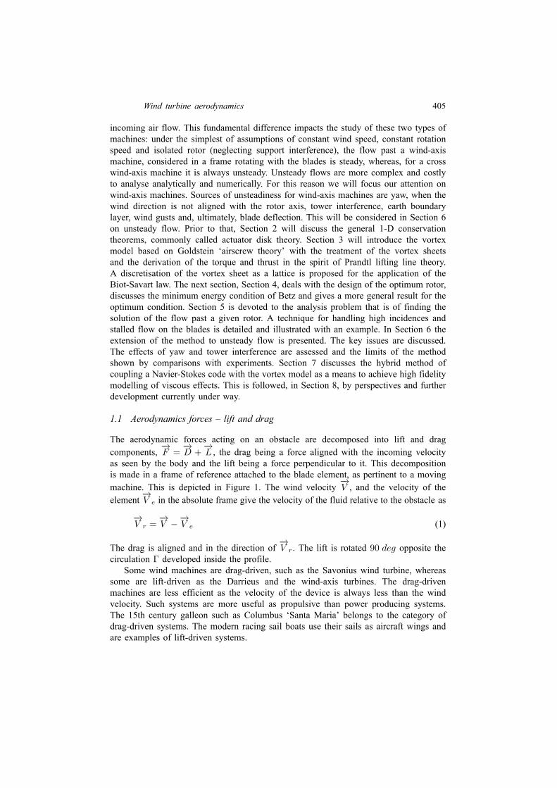
incoming air flow. This fundamental difference impacts the study of these two types ofmachines: under the simplest of assumptions of constant wind speed, constant rotationspeed and isolated rotor (neglecting support interference), the flow past a wind-axismachine, considered in a frame rotating with the blades is steady, whereas, for a crosswind-axis machine it is always unsteady. Unsteady flows are more complex and costlyto analyse analytically and numerically. For this reason we will focus our attention onwind-axis machines. Sources of unsteadiness for wind-axis machines are yaw, when thewind direction is not aligned with the rotor axis, tower interference, earth boundarylayer, wind gusts and, ultimately, blade deflection. This will be considered in Section 6on unsteady flow. Prior to that, Section 2 will discuss the general 1-D conservationtheorems, commonly called actuator disk theory. Section 3 will introduce the vortexmodel based on Goldstein ‘airscrew theory’ with the treatment of the vortex sheetsand the derivation of the torque and thrust in the spirit of Prandtl lifting line theory.A discretisation of the vortex sheet as a lattice is proposed for the application of theBiot-Savart law. The next section, Section 4, deals with the design of the optimum rotor,discusses the minimum energy condition of Betz and gives a more general result for theoptimum condition. Section 5 is devoted to the analysis problem that is of finding thesolution of the flow past a given rotor. A technique for handling high incidences andstalled flow on the blades is detailed and illustrated with an example. In Section 6 theextension of the method to unsteady flow is presented. The key issues are discussed.The effects of yaw and tower interference are assessed and the limits of the methodshown by comparisons with experiments. Section 7 discusses the hybrid method ofcoupling a Navier-Stokes code with the vortex model as a means to achieve high fidelitymodelling of viscous effects. This is followed, in Section 8, by perspectives and furtherdevelopment currently under way.

1.1 Aerodynamics forces – lift and drag

The aerodynamic forces acting on an obstacle are decomposed into lift and dragcomponents,

−→F =

−→D +

−→L , the drag being a force aligned with the incoming velocity

as seen by the body and the lift being a force perpendicular to it. This decompositionis made in a frame of reference attached to the blade element, as pertinent to a movingmachine. This is depicted in Figure 1. The wind velocity

−→V , and the velocity of the

element−→V e in the absolute frame give the velocity of the fluid relative to the obstacle as

−→V r =

−→V −

−→V e (1)

The drag is aligned and in the direction of−→V r. The lift is rotated 90 deg opposite the

circulation Γ developed inside the profile.Some wind machines are drag-driven, such as the Savonius wind turbine, whereas

some are lift-driven as the Darrieus and the wind-axis turbines. The drag-drivenmachines are less efficient as the velocity of the device is always less than the windvelocity. Such systems are more useful as propulsive than power producing systems.The 15th century galleon such as Columbus ‘Santa Maria’ belongs to the category ofdrag-driven systems. The modern racing sail boats use their sails as aircraft wings andare examples of lift-driven systems.

406 J-J. Chattot

Figure 1 Lift and drag forces acting on a moving blade element

x

z

V×

i×

k×

Ve×ÖÖÖ

-Ve×ÖÖÖVr

×ÖÖÖ

D×

L×

G<0

A drag-driven device rotating about the y-axis (into the paper in Figure 1) willcorrespond to

−→V e ≃ Ve

−→i where Ve < V and the lift force is either zero or does not

contribute to the power P =−→F .

−→V ≃ DV .

A lift-driven device rotating about the x-axis (wind-axis turbine) will correspondto

−→V e ≃ −Ve

−→k and with (L/D)max ≃ 10 the lift force will be the component

contributing primarily to power generation.

1.2 Savonius rotor

According to Wikipedia:

“Savonius wind turbines are a type of vertical-axis wind turbine (VAWT), used forconverting the power of the wind into torque on a rotating shaft. They were inventedby the Finnish engineer Sigurd J. Savonius in 1922. Johann Ernst Elias Bessler (born1680) was the first to attempt to build a horizontal windmill of the Savonius type inthe town of Furstenburg in Germany in 1745. He fell to his death whilst constructionwas under way. It was never completed but the building still exists.

Savonius turbines are one of the simplest turbines. Aerodynamically, they are drag-typedevices, consisting of two or three scoops. Looking down on the rotor from above,a two-scoop machine would look like an ‘S’ shape in cross section. Because of thecurvature, the scoops experience less drag when moving against the wind than whenmoving with the wind. The differential drag causes the Savonius turbine to spin.Because they are drag-type devices, Savonius turbines extract much less of the wind’spower than other similarly-sized lift-type turbines. Much of the swept area of a Savoniusrotor is near the ground, making the overall energy extraction less effective due tolower wind speed at lower heights.


Savonius turbines are used whenever cost or reliability is much more important thanefficiency. For example, most anemometers are Savonius turbines, because efficiencyis completely irrelevant for that application. Much larger Savonius turbines have beenused to generate electric power on deep-water buoys, which need small amounts ofpower and get very little maintenance. Design is simplified because, unlike horizontalaxis wind turbines (HAWTs), no pointing mechanism is required to allow for shiftingwind direction and the turbine is self-starting. Savonius and other vertical-axis machinesare not usually connected to electric power grids. They can sometimes have long helicalscoops, to give smooth torque.

The most ubiquitous application of the Savonius wind turbine is the Flettner Ventilatorwhich is commonly seen on the roofs of vans and buses and is used as a coolingdevice. The ventilator was developed by the German aircraft engineer Anton Flettnerin the 1920s. It uses the Savonius wind turbine to drive an extractor fan. The ventsare still manufactured in the UK by Flettner Ventilator Limited.

Small Savonius wind turbines are sometimes seen used as advertising signs where therotation helps to draw attention to the item advertised.” (See Figure 2)

Figure 2 Schematic drawings and operation of a two-scoop Savonius turbine

1.3 Darrieus rotor

According to Wikipedia:

“The Darrieus wind turbine is a type of vertical axis wind turbine (VAWT) used togenerate electricity from the energy carried in the wind. The turbine consists of anumber of aerofoils vertically mounted on a rotating shaft or framework. This designof wind turbine was patented by Georges Jean Marie Darrieus, a French aeronauticalengineer in 1931.

The Darrieus type is theoretically just as efficient as the propeller type if wind speedis constant, but in practice this efficiency is rarely realised due to the physical stressesand limitations imposed by a practical design and wind speed variation. There are alsomajor difficulties in protecting the Darrieus turbine from extreme wind conditions andin making it self-starting.

In the original versions of the Darrieus design, the aerofoils are arranged so that theyare symmetrical and have zero rigging angle, that is, the angle that the aerofoils areset relative to the structure on which they are mounted. This arrangement is equallyeffective no matter which direction the wind is blowing – in contrast to the conventionaltype, which must be rotated to face into the wind.

408 J-J. Chattot

When the Darrieus rotor is spinning, the aerofoils are moving forward through the airin a circular path. Relative to the blade, this oncoming airflow is added vectorially tothe wind, so that the resultant airflow creates a varying small positive angle of attack(AoA) to the blade. This generates a net force pointing obliquely forwards along acertain ‘line-of-action’. This force can be projected inwards past the turbine axis at acertain distance, giving a positive torque to the shaft, thus helping it to rotate in thedirection it is already travelling in. The aerodynamic principles which rotates the rotorare equivalent to that in autogiros, and normal helicopters in autorotation.

As the aerofoil moves around the back of the apparatus, the angle of attack changes tothe opposite sign, but the generated force is still obliquely in the direction of rotation,because the wings are symmetrical and the rigging angle is zero. The rotor spins ata rate unrelated to the windspeed, and usually many times faster. The energy arisingfrom the torque and speed may be extracted and converted into useful power by usingan electrical generator.

The aeronautical terms lift and drag are, strictly speaking, forces across and along theapproaching net relative airflow respectively, so they are not useful here. We reallywant to know the tangential force pulling the blade around, and the radial force actingagainst the bearings.

When the rotor is stationary, no net rotational force arises, even if the wind speedrises quite high – the rotor must already be spinning to generate torque. Thus thedesign is not normally self starting. It should be noted though, that under extremelyrare conditions, Darrieus rotors can self-start, so some form of brake is required to holdit when stopped (see Figure 3).

One problem with the design is that the angle of attack changes as the turbine spins, soeach blade generates its maximum torque at two points on its cycle (front and back ofthe turbine). This leads to a sinusoidal (pulsing) power cycle that complicates design.In particular, almost all Darrieus turbines have resonant modes where, at a particularrotational speed, the pulsing is at a natural frequency of the blades that can cause themto (eventually) break. For this reason, most Darrieus turbines have mechanical brakesor other speed control devices to keep the turbine from spinning at these speeds forany lengthy period of time ...

... In overall comparison, while there are some advantages in Darrieus design there aremany more disadvantages, especially with bigger machines in MW class. The Darrieusdesign uses much more expensive material in blades while most of the blade is toonear of ground to give any real power. Traditional designs assume that wing tip is atleast 40 m from ground at lowest point to maximise energy production and life time.So far, there is no known material (not even carbon fiber) which can meet cyclic loadrequirements.”

1.4 Horizontal axis wind turbine

In the rest of the chapter, the attention will be devoted to HAWTs which represent,today, the main type of wind power machines that are developed and installed in allparts of the world. Much efforts have been done in understanding better the flow pastHAWT both experimentally and analytically. A major wind tunnel campaign has beencarried out by the National Renewable Energy Laboratory (NREL) at the NASA AmesResearch Centre large 80’ × 120’ wind tunnel facility (Hand et al., 2001). They useda two-bladed rotor of radius R = 5 m with blades equipped with the S809 profile. Apicture of the wind turbine in the wind tunnel is shown in Figure 4. Note in particularthe well defined evolution of the tip vortex visualised with smoke emitted from the


tip of one blade. One can count seven or eight turns with regular spacing, despite thedramatic distortion due to the encounter with the tower when the blade tip vortex passesin front of it.

Figure 3 Schematic of a Darrieus turbine (see online version for colours)

Figure 4 NREL turbine in NASA Ames 80’ × 120’ wind tunnel (see online version for colours)

410 J-J. Chattot

2 General 1-D conservation theorems – actuator disk theory

As a first-order approximation, the flow past a HAWT is treated as quasi-onedimensional. The stream tube captured by the rotor is described by its cross-sectionA(x) and the velocity

−→V = (U + u, v, w) representing the uniform flow plus a

perturbation (u, v, w) in cylindrical coordinates. At the rotor disk, the velocity iscontinuous, but the pressure is allowed to jump, as if the rotor had infinitely manyblades and was equivalent to a porous disk. The stream tube boundary downstream ofthe disk allows for a discontinuity in axial velocity between the flow inside and outsidethe stream tube, called slip stream. As a further simplification, the flow rotation behindthe rotor is neglected, hence the azimuthal velocity component is zero (w = 0).

Consider a cylindrical control volume/control surface Σ3 with large diameter,containing the captured stream tube and bounded by two disks far upstream Σ1 and fardownstream Σ2 located in what is called the Trefftz plane, see Figure 5. At the upstreamboundary, the incoming flow is uniform and undisturbed with velocity U aligned withthe turbine axis, and pressure p∞. Downstream, at the Trefftz plane, the pressure returnsto p∞, but the velocity inside the stream tube is less than the undisturbed value Uoutside of it. The flow is considered steady, incompressible (ρ = const.) and inviscid.Application of the conservation laws to the control volume/control surface yields theresults known as Rankine-Froude (Rankine, 1865; Froude, 1889) or actuator disk theory.

Figure 5 Control volume/control surface for conservation theorems

x

CSCV

U U+u U+u2

S1 S2

S3

S3

p¥ p¥

n×1 n×2

n×3

n×3

A1A A2

T×

The conservation of mass (volume flow) reads:∫CS

(−→V .−→n )dA = 0 (2)

which can be broken into the various control surface contributions as

(−U)Σ1 + (U)(Σ2 −A2) + (U + u2)A2 +

∫Σ3

(−→V .−→n )dA = 0 (3)


The cross section of the control volume is constant, hence Σ1 = Σ2. Aftersimplification, this reduces to

u2A2 +

∫Σ3

(−→V .−→n )dA = 0 (4)

which means that the deficit or excess of volume flow through the exit section iscompensated by the flow across the lateral surface of the cylinder. The conservation ofx-momentum reads∫

CS

ρ(U + u)(−→V .−→n )dA = −

∫CS

pnxdA− T (5)

where T represents the thrust exerted by the flow on the rotor/actuator disk. This isexpanded as

ρU(−U)Σ1 + ρ(U)2(Σ2 −A2) + ρ(U + u2)2A2 +

∫Σ3

ρU(−→V .−→n )dA = −T (6)

Note that, since pressure is constant and equal to p∞ on all control surfaces, it doesnot contribute to the momentum balance. The last term on the left-hand-side can beevaluated using the result of mass conservation. Solving for T :

T = −ρ(U + u2)u2A2 = −mu2 (7)

where m = ρ(U + u)A = const. represents the mass flow rate in the stream tube andA = πR2, R denotes the radius of the rotor . Note that, since T > 0, then u2 < 0 for aturbine.

The steady energy equation applies to the stream tube with one-dimensional entranceand exit sections:∫

A1

(p

ρ+V 2

2+ gz

)dm =

∫A2

(p

ρ+V 2

2+ gz

)dm− Ws (8)

Ws = P represents the shaft work or power extracted (P < 0) from the flow by therotor. Solving for P

P =

(p∞ρ

+(U + u2)

2

2

)m−

(p∞ρ

+U2

2

)m (9)

After simplifying the above expression one finds

P =(U +

u22

)mu2 (10)

The power is also given by P = −T (U + u) = (U + u)mu2. From this, we concludethat u2 = 2u.

Results of this analysis can be summarised in terms of the rotor/actuator diskparameters

412 J-J. Chattot

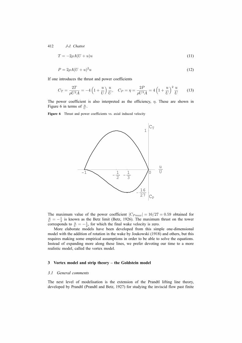
T = −2ρA(U + u)u (11)

P = 2ρA(U + u)2u (12)

If one introduces the thrust and power coefficients

CT =2T

ρU2A= −4

(1 +

u

U

) u

U, CP = η =

2P

ρU3A= 4

(1 +

u

U

)2 u

U(13)

The power coefficient is also interpreted as the efficiency, η. These are shown inFigure 6 in terms of u

U .

Figure 6 Thrust and power coefficients vs. axial induced velocity

-1-12-13

0uU

-1627

1CT

CP

The maximum value of the power coefficient |CPmax| = 16/27 = 0.59 obtained foruU = −1

3 is known as the Betz limit (Betz, 1926). The maximum thrust on the towercorresponds to u

U = − 12 , for which the final wake velocity is zero.

More elaborate models have been developed from this simple one-dimensionalmodel with the addition of rotation in the wake by Joukowski (1918) and others, but thisrequires making some empirical assumptions in order to be able to solve the equations.Instead of expanding more along these lines, we prefer devoting our time to a morerealistic model, called the vortex model.

3 Vortex model and strip theory – the Goldstein model

3.1 General comments

The next level of modelisation is the extension of the Prandtl lifting line theory,developed by Prandtl (Prandtl and Betz, 1927) for studying the inviscid flow past finite


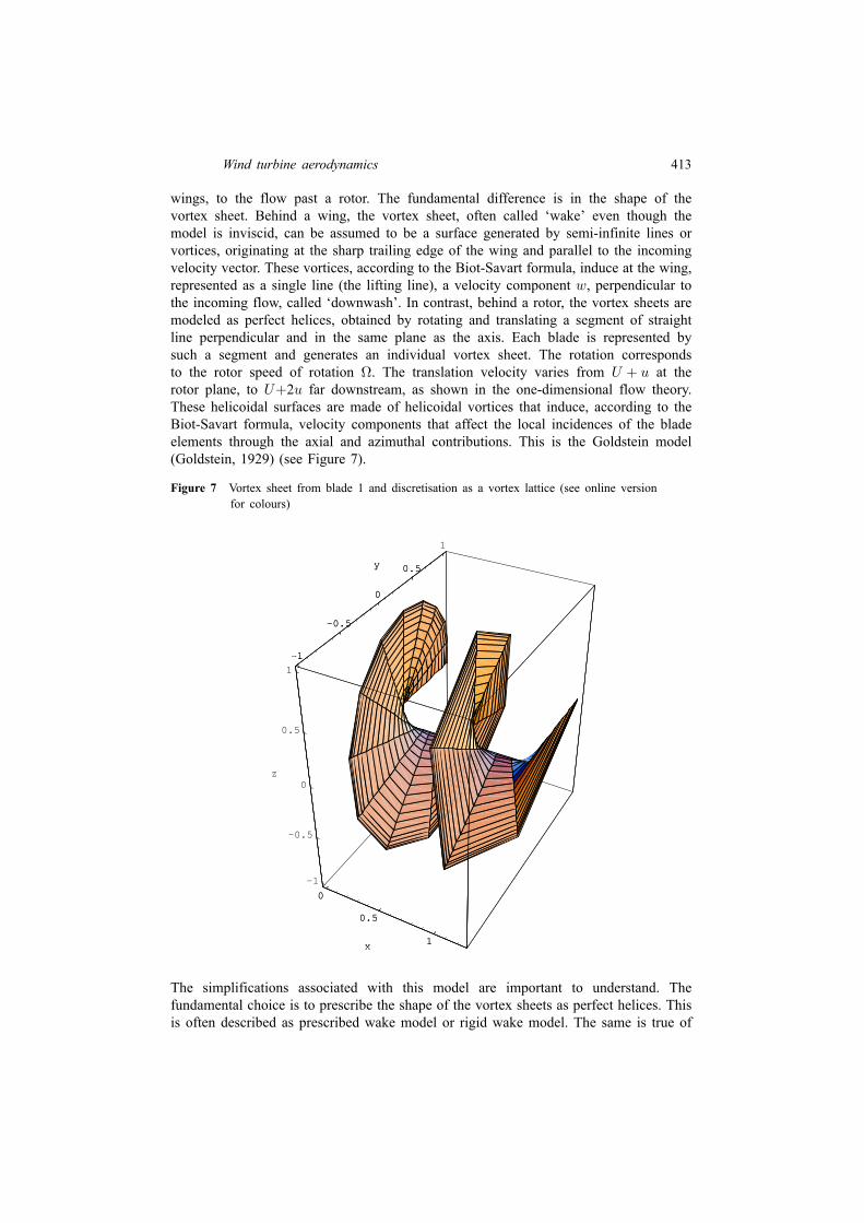
wings, to the flow past a rotor. The fundamental difference is in the shape of thevortex sheet. Behind a wing, the vortex sheet, often called ‘wake’ even though themodel is inviscid, can be assumed to be a surface generated by semi-infinite lines orvortices, originating at the sharp trailing edge of the wing and parallel to the incomingvelocity vector. These vortices, according to the Biot-Savart formula, induce at the wing,represented as a single line (the lifting line), a velocity component w, perpendicular tothe incoming flow, called ‘downwash’. In contrast, behind a rotor, the vortex sheets aremodeled as perfect helices, obtained by rotating and translating a segment of straightline perpendicular and in the same plane as the axis. Each blade is represented bysuch a segment and generates an individual vortex sheet. The rotation correspondsto the rotor speed of rotation Ω. The translation velocity varies from U + u at therotor plane, to U+2u far downstream, as shown in the one-dimensional flow theory.These helicoidal surfaces are made of helicoidal vortices that induce, according to theBiot-Savart formula, velocity components that affect the local incidences of the bladeelements through the axial and azimuthal contributions. This is the Goldstein model(Goldstein, 1929) (see Figure 7).

Figure 7 Vortex sheet from blade 1 and discretisation as a vortex lattice (see online versionfor colours)

0

0.5

1x

-1

-0.5

0

0.5

1

y

-1

-0.5

0

0.5

1

z

0

0.5

1x

-1

-0.5

0

0.5y

The simplifications associated with this model are important to understand. Thefundamental choice is to prescribe the shape of the vortex sheets as perfect helices. Thisis often described as prescribed wake model or rigid wake model. The same is true of

414 J-J. Chattot

the wake model in Prandtl lifting line theory, which is aligned with the undisturbedflow, yet yields very reasonable results. From a physical point of view, vortex sheetsare surfaces of discontinuity of the velocity vector, wetted on both sides by the fluidand find an equilibrium position such that the pressure is continuous across them. Froma practical point of view, if the prescribed vortex sheets are close to the actual ones,the evaluation of the induced velocities will be accurate to first-order, as is the case inPrandtl theory and in the transfer of the tangency condition from the actual profile to thenearby axis in small disturbance theory of thin airfoils. In this method, the prescribedvortex structure satisfies an ‘equilibrium condition’ by matching the absorbed rotorpower with the power deficit in the far field, as will be seen later.

Another simplification consists in neglecting the rolling-up of the sheets edges, awell-known phenomena in aircraft aerodynamics associated with tip vortices that cancreate a hazard for small aircrafts flying in the tip vortices wake of large transportairplanes. Results indicate that keeping the sheets flat does not affect the accuracy ofthe simulation since the rolling-up does not change the vorticity content of the wake,only displaces it slightly.

The average axial velocity decreases behind the rotor. As a consequence, the streamtube diameter increases. The helicoidal vortex sheets would be expected to expand,however, this is not accounted for and possibly does not need to, since the rolling up ofthe sheets edges may counter this effect. It is believed that the rolling-up of the vortexsheets as well as the stream tube expansion are second-order effects, hence neglectingto account for them does not jeopardise the results.

The centrifugal and Coriolis forces are also neglected, which is acceptable for largewind turbines.

Free wake models have been developed in which the vortex sheets are allowed tofind their equilibrium position as part of a Lagrangian iterative process in which vorticityis shed by the blades and convected downstream. Experience has shown that thesemethods are unstable. The vortex filaments tend to become disorganised and chaoticdownstream of the rotor. Artificial dissipation is needed to prevent the calculationfrom diverging, which defeats the purpose of keeping the wake dissipation free, asexpected with an inviscid model. Another aspect is that the number of vorticity ladenparticles increases with each time step and the run time per iteration increases quicklyto excessive values as N3, where N is the number of particles. In the end, the freewake models are neither reliable nor efficient.

3.2 Discretisation of the vortex sheets

Consider a rotor rotating at speed Ω, placed in an incoming uniform flow with velocityV = (U, 0, 0) aligned with the turbine axis. We neglect the tower interference on therotor flow. In a frame of reference attached to the rotor, the flow is steady. The tip speedratio is defined as TSR = ΩR/U = 1/adv, which is also the inverse of the advanceratio, adv used as main parameter for propellers. Other dimensionless quantities aredefined and used below:

x = Rx, y = Ry, z = Rz (14)

c = Rc (15)

u = Uu, v = Uv, w = Uw (16)


Γ = URΓ (17)

T =π

2ρU2R2CT , τ =

π

2ρU2R3Cτ , L

′ =1

2ρU2RcCl (18)

The ‘-’ values correspond to dimensional quantities. T is the thrust on the tower (N ),CT the thrust coefficient, τ is the torque (N.m), Cτ the torque coefficient, L′ is thelocal lift force per unit span, and Cl is the local lift coefficient.

Each vortex sheet such as that in Figure 7 is discretised as a lattice shown unrolledin Figure 8 to better explain the numerical scheme.

Figure 8 Schematic representation of a vortex sheet

x

yj=1 1i=123

i

i-1

2 j j+1

ix

0

ë

ë ë

Gi-1,j

Gi,j Gi,j+1

dl×ÖÖÖÖ

The circulation Γi,j is located at the grid points of the lattice (indicated by the circles).The blade is represented by a lifting line along the y-axis for blade 1 (thick solid line)and Γ1,j represents the circulation inside the blade. The small elements of vorticity

−→dl

are located between the grid points and correspond either to trailed vorticity (in thex-direction in the presentation of Figure 8) or shed vorticity (in the y-direction) thatis present only when the flow is unsteady. When the flow is steady, as assumed here,the circulation is constant along a vortex filament, i.e., Γi,j = Γ1,j , ∀i = 2, ..., ix. Thevorticity is given in terms of the differences in circulation as ∆Γi,j = Γi,j+1 − Γi,j forthe trailed vorticity and ∆Γi,j = Γi,j − Γi−1,j (= 0 here) for shed vorticity. The vortexelement orientation is indicated by the arrow which represents positive ∆Γi,j but thevector components account for the rolling of the sheet on a perfect helix. Let xi, yi, zirepresent the tip vortex of blade 1

The advance ratio is made to vary linearly from adv1 = (V + u)/ΩR at the rotorplane i = 1 to advix = (V + 2u)/ΩR after a few turns of the helix, then remains

416 J-J. Chattot

constant thereafter to the Trefftz plane i = ix. The mesh distribution in the x-directionis stretched from an initial value dx1 at the blade, to some location xstr ≃ 1, using astretching parameter s > 1 as

xi = xi−1 + dxi−1, dxi = sdxi−1, i = 2, ..., ix (19)

yi = cos(

xiadvi

), zi = sin

(xiadvi

)(20)

Beyond x = xstr the mesh is uniform all the way to the Trefftz plane xix ≃ 20.In the y-direction, the mesh is discretised with a cosine distribution

yj = y0 +1

2(1− y0) cos θj , θj =

j − 1

jx− 1π, j = 1, ..., jx (21)

The trailed vortices are located between the mesh lines according to

ηj = y0 +1

2(1− y0) cos θj , θj =

2j − 1

2(jx− 1)π, j = 1, ..., jx− 1 (22)

Accounting for the rolling of the sheet on a perfect helix, a small element of trailedvorticity has components

−→dl = dxi, dyi,j , dzi,j

=− 1

2 (xi+1 − xi−1),− 12 (yi+1 − yi−1)ηj ,−1

2 (zi+1 − zi−1)ηj (23)

whereas, a small element of shed vorticity has components

−→dl = dxi, dyi,j , dzi,j

=0, 12 (yi−1 + yi)(ηj − ηj−1),

12 (zi−1 + zi)(ηj − ηj−1)

(24)

Application of the Biot-Savart formula provides the influence coefficients for the smallelements, which are accumulated and stored in multidimensional arrays.

A particular treatment is made for the trailed elements closest to the lifting lineand at the Trefftz plane. The former extend only half a cell with origin at 1

2 (x1 + x2)(see Figure 8), and the latter extend from ∞ to 1

2 (xix−1 + xix), where a remainderaccounts for the contribution downstream of the Trefftz plane. Note that in the case ofthe three-bladed rotor, the lifting lines themselves induce velocities on the other two (butnot on themselves as straight blades). The same discretisation applies for the calculationof the lifting line contributions for a three-bladed rotor, but now the small vortex elementis located along the lifting line, having components

−→dl = 0, ηj − ηj−1, 0 , j = 2, ..., jx− 1 (25)

in the case of blade 1, and ∆Γi,j = Γ1,j represents the circulation inside the blade.


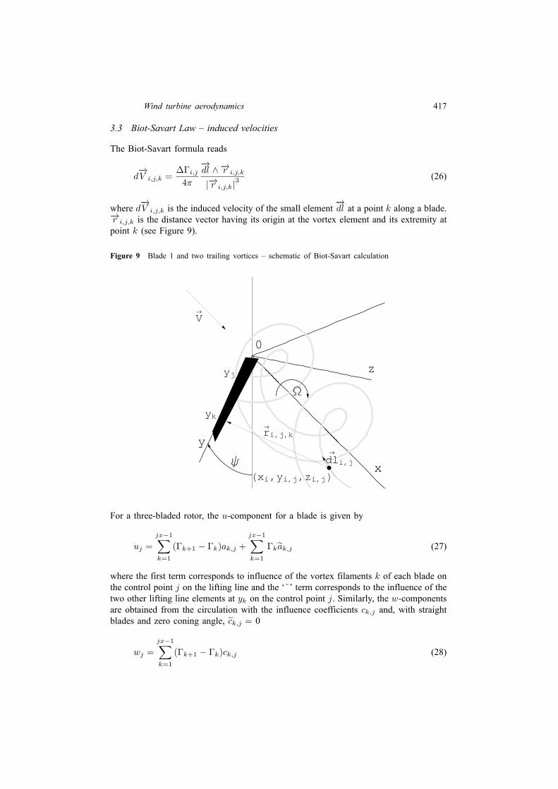
3.3 Biot-Savart Law – induced velocities

The Biot-Savart formula reads

d−→V i,j,k =

∆Γi,j

4π

−→dl ∧ −→r i,j,k

|−→r i,j,k|3 (26)

where d−→V i,j,k is the induced velocity of the small element

−→dl at a point k along a blade.

−→r i,j,k is the distance vector having its origin at the vortex element and its extremity atpoint k (see Figure 9).

Figure 9 Blade 1 and two trailing vortices – schematic of Biot-Savart calculation

0

V®

x

y

z

Ψ

W

dl®

i,j

r®

i,j,k

Hxi,yi,j,zi,jL

yj

yk

For a three-bladed rotor, the u-component for a blade is given by

uj =

jx−1∑k=1

(Γk+1 − Γk)ak,j +

jx−1∑k=1

Γkak,j (27)

where the first term corresponds to influence of the vortex filaments k of each blade onthe control point j on the lifting line and the ‘˜’ term corresponds to the influence of thetwo other lifting line elements at yk on the control point j. Similarly, the w-componentsare obtained from the circulation with the influence coefficients ck,j and, with straightblades and zero coning angle, ck,j = 0

wj =

jx−1∑k=1

(Γk+1 − Γk)ck,j (28)

418 J-J. Chattot

Given the induced velocity components, the flow at the blade element can be analysedand the local lift found. This is an approximation that amounts to neglecting the effectof the neighbouring elements and considers each element in isolation, as if it were partof an infinite blade. Mathematically, this corresponds to neglecting the derivatives inthe span direction compared to the other derivatives: ∂

∂y ≪ ∂∂x ,

∂∂z . This is appropriate,

as has been found, for large aspect ratio wings and blades, that is those for which thechord is small compared to the span. This approach is called ‘strip theory’.

Figure 10 Blade element flow configuration

x

z

01+uj

yjadv

+wj

qj

qj

tj Φj

Αj

L×

j

’G<0

3.4 Forces and moment

The flow is assumed to be inviscid, Cd = 0. At the blade element j the flowconfiguration is as depicted in Figure 10.

The local incidence is

αj = ϕj − tj = arctan(

1 + ujyj

adv + wj

)− tj (29)

where ϕj is called the flow angle and tj is the angle of twist at the element. The locallift coefficient is obtained from the result of thin airfoil theory or from an experimentalor numerical profile lift curve Cl(α). In thin airfoil theory, the lift is given by

Cl(α) = 2π(α+ 2d

c) (30)

dc is the profile mean camber defined as

d

c=

1

2π

∫ 1

0

d′(x)1− 2x

c√xc (1−

xc )

dx

c(31)

where d(x) is the equation of the camber line. According to the Kutta-Joukowskilift theorem, the lift force per unit span is perpendicular to the incoming flow,


its magnitude is L′ = ρqΓ and its orientation is 90 deg from the incoming flow

direction, rotating opposite to the circulation. q = qU =

√(1 + u)

2+

(y

adv + w)2 is the

normalised magnitude of the incoming flow velocity vector. This can be expressedmathematically as

−→L ′ = ρU−→q ∧ URΓ−→j (32)

where dimensionless quantities have been introduced.−→j is the unit vector along the

y-axis and Γ < 0 in Figure 10. Upon adimensionalisation of the lift, the circulation isobtained as

Γj = −1

2qjcjCl(αj) (33)

The contribution of the blade element to thrust and torque can now be derived.Projection in the x-direction gives

dTj = L′j cosϕjRdyj

= −ρUqj cosϕjURΓjRdyj = −ρU2R2Γj

( yj

adv + wj

)dyj (34)

or, upon integration

T = −ρU2R2

∫ 1

y0

Γ(y)( y

adv+ w(y)

)dy (35)

In dimensionless form

CT =T

12ρU

2πR2= − 2

π

∫ 1

y0

Γ(y)( y

adv+ w(y)

)dy (36)

Projection of the lift force in the z-direction and accounting for the distance from theaxis, the torque contribution reads

dτj =L′j sinϕjRyjRdyj

=Uqj sinϕjURΓjRyjRdyj=U2R3Γj (1 + uj) yjdyj

(37)

which integrates to give

τ = ρU2R3

∫ 1

y0

Γ(y) (1 + u(y)) ydy (38)

or, in dimensionless form

Cτ =τ

12ρU

2πR3=

2

π

∫ 1

y0

Γ(y) (1 + u(y)) ydy (39)

These results are for one blade. Total thrust and torque must account for all the blades.

420 J-J. Chattot

3.5 Wake equilibrium condition

The power absorbed by the rotor is also estimated by using the torque evaluation andthe speed of rotation as

P = τΩ (40)

The vortex sheets are considered in ‘equilibrium’ when the power absorbed by the rotormatches the power deficit Ws in the far wake obtained from actuator disk theory, i.e.,with the current notation

P = τΩ = 2πρU3R2(1 + u)2u (41)

This is a cubic equation for the average axial induced velocity u at the rotor

4(1 + u)2u = TSR Cτ =Cτ

adv= CP (42)

The solution procedure consists in recalculating the solution with an updatedvortex structure until it satisfies the equilibrium condition to acceptable accuracy(|∆Cτ/Cτ | ≤ 10−3).

4 Aerodynamic design of a rotor blade – Betz minimum energy condition

4.1 Formulation

The minimum energy condition of Betz (1919) refers to the optimum conditions whichlead to the minimum loss of energy in the slipstream. It applies equally to propellersand wind turbines. For the latter, the optimum distribution of circulation Γ(y) minimisesthe torque (negative) for a given thrust on the tower. The simple argument of Betz isthat, in this case, an elementary force δCT = − 2

πΓ(y)(

yadv + w(y)

)dy should produce

a constant elementary torque δCτ = 2πΓ(y) (1 + u(y)) ydy, independent of y. Hence the

minimum energy condition of Betz reads

(1 + u(y)) yy

adv + w(y)= y tanϕ(y) = const. (43)

This is true only for vanishing circulation and induced velocities, as will be shown later.By analogy, lets consider the problem of the optimum wing loading in Prandtl liftingline theory. Given that the lift and induced drag are

CL = 2

∫ 1

−1

Γ(y)dy, CDi = −∫ 1

−1

Γ(y)w(y)dy (44)

where w(y) is the downwash (negative),

w(y) = − 1

4π

∫ 1

−1

Γ′(η)dη

y − η(45)


Munk (1921) showed that, for the optimum loading, the downwash w has to be constant,else, moving a small element of lift (elementary horseshoe vortex) δCL = 2δΓdy fromits current position y1 to a position y2 such that δw = w(y2)− w(y1) > 0, would notchange the total lift, yet would change the induced drag by δCDi = −2δΓδwdy < 0,a decrease in total drag, indicating that the distribution is not optimal. In other words,for an elementary δCL = 2Γdy, the induced drag δCDi = −2Γ(y)w(y)dy should beindependent of y, which implies that w(y) = const. A more mathematical proof consistsin considering the objective function

F (Γ) = CDi(Γ) + λCL(Γ) (46)

consisting of the induced drag to be minimised for a given lift, where λ is the Lagrangemultiplier. Taking the Frechet derivative yields the minimisation equation that must holdfor any change δΓ of circulation. The Frechet derivative can be defined as the limitingprocess

∂F

∂Γ(δΓ) = lim

θ→0

d

dθF (Γ + θδΓ) (47)

The result is linear in δΓ. It represents the derivative of F with respect to Γ, in thedirection of δΓ. Here we obtain:

∂F

∂Γ(δΓ) = −

∫ 1

−1

(δΓ(y)w(y) + Γ(y)

∂w

∂Γ(δΓ)

)dy + 2λ

∫ 1

−1

δΓ(y)dy (48)

But the kernel of w(Γ) is antisymmetric. Hence, integration by part twice using the factthat Γ(±1) = δΓ(±1) = 0, yields the identity

Γ(y)∂w

∂Γ(δΓ) = δΓw(Γ) (49)

Indeed, consider the second term in the integral above. By definition of the Frechetderivative of w(Γ) in the direction δΓ

I = −∫ 1

−1

Γ(y)∂w

∂Γ(δΓ)dy = −

∫ 1

−1

Γ(y)

(− 1

4π

∫ 1

−1

δΓ′(η)dη

y − η

)dy (50)

I =1

4π

∫ 1

−1

∫ 1

−1

Γ(y)δΓ′(η)dηdy

y − η(51)

A first integration by parts in η yields

I =1

4π

∫ 1

−1

[Γ(y)δΓ(η)

y − η

]1−1

−∫ 1

−1

Γ(y)δΓ(η)dη

(y − η)2

dy (52)

The integrated term vanishes to leave after a second integration by parts in y

I = − 1

4π

∫ 1

−1

[−δΓ(η)Γ(y)

y − η

]1−1

+

∫ 1

−1

δΓ(η)Γ′(y)dy

y − η

dη (53)

422 J-J. Chattot

Again, the integrated term vanishes and the second term, thanks to the antisymmetry ofthe kernel 1

y−η , can be interpreted as

I = −∫ 1

−1

δΓ(η)

− 1

4π

∫ 1

−1

Γ′(y)dy

η − y

dη = −

∫ 1

−1

δΓ(η)w(η)dη (54)

Finally, the minimisation equation reduces to

∂F

∂Γ(δΓ) = −2

∫ 1

−1

δΓ(y) (w(y)− λ) dy, ∀δΓ (55)

The solution is simply w(y) = λ = const., as obtained by Munk with his simplerargument. The antisymmetry of the kernel simply indicates that two elementaryhorseshoe vortices of same intensity placed at y1 and y2 induce downwash that areopposite at the other horseshoe location. This is not the case with a wind turbine wake,because two vortices along the helix will have different shapes depending on their initialy-location at the blade, hence induced velocities u or w are not related. Let yv, zv bethe equation of the vortex sheet of blade 1yv = η cos

(x

adv(x)

)zv = η sin

(x

adv(x)

) (56)

A vortex filament corresponds to a fixed value of η. Two such vortices are shown inFigure 9.

The kernel for u and w does not have the antisymmetry property for the helicoidalvortex sheet as can be seen from the formula

u(y) =

∫ 1

y0

∫ ∞

0

Γ′(η)

4π

(y − yv)dzvdx + zv

dyv

dx

[x2 + (y − yv)2 + z2v ]32

dxdη (57)

w(y) = −∫ 1

y0

∫ ∞

0

Γ′(η)

4π

(y − yv) + xdyv

dx

[x2 + (y − yv)2 + z2v ]32

dxdη (58)

The objective function for the optimum turbine blade reads

F (Γ) = Cτ (Γ) + λCT (Γ) (59)

stating that the search is for minimum torque (negative) for a given thrust on the towerat a given tip speed ratio and blade root location y0. The minimisation equation isderived for one blade as

∂F

∂Γ(δΓ) =

2

π

∫ 1

y0

δΓ (1 + u(y)) y + Γ(y)

∂u

∂Γ(δΓ)

dy

−2λ

π

∫ 1

y0

δΓ

( y

adv+ w(y)

)+ Γ(y)

∂w

∂Γ(δΓ)

dy (60)


= 0, ∀δΓThe terms such as Γ(y) ∂u∂Γ (δΓ) cannot be transformed in this case, however, choosingδΓ = Γ yields the following identity∫ 1

y0

Γ(1 + 2u(y)) y − λ

( y

adv+ 2w(y)

)dy = 0 (61)

the interpretation of which is that the optimum solution satisfies the minimum energycondition of Betz, in the Trefftz plane, ‘in the average’, with Γ as weighting factor.For a tip speed ratio TSR = 2.9, the design of a two bladed-rotor at (Cl)opt =0.8979with very light loading demonstrates that the minimum energy condition of Betzis verified. The thrust coefficient is CT = 0.0032, the corresponding value of theLagrange multiplier is λ = 0.3433 and the power coefficient CP = 0.0031. For ahigher loading, corresponding to the two-bladed NREL rotor at the same TSR andCT = 0.205, one finds λ = 0.254 and CP = 0.1768. The deviation from the Betzcondition, e(y) = (y tanϕ(y)− λ)/λ, is shown in Figure 11. As can be seen, for lightlyloaded rotor, the Betz condition is satisfied, but it is no longer the case when loading ismore realistic.

Figure 11 Verification of Betz condition for two design examples at TSR = 2.9

0.2 0.4 0.6 0.8 1

y

−0.1

−0.05

0

0.05

0.1

0.15

0.2

e(y)

CT=0.0032jx=21jx=51jx=101CT=0.205jx=21jx=51jx=101

4.2 Discretisation

The discrete formulation is now described. The influence coefficients are calculated as

aj,k or aj,k =1

4π

ix∑i=2

(yk − yi,j)dzi,j + zi,jdyi,j[x2i + (yk − yi,j)2 + z2i,j

] 32

(62)

424 J-J. Chattot

cj,k = − 1

4π

ix∑i=2

(yk − yi,j)dxi + xidyi,j[x2i + (yk − yi,j)2 + z2i,j

] 32

(63)

with the notation introduced earlier and in Figure 9. The contributions to aj,k and cj,kof the vortex filament part that is beyond the Trefftz plane are approximated by thefollowing remainders

δaj,k =1

4π

∫ ∞

xix

(y − yv)dzvdx + zv

dyv

dx

[x2 + (y − yv)2 + z2v ]32

dx

≃− 1

4π

yk − 2ηj cos(

xix

advix

)2x2ix

+O

(1

x3ix

) (64)

δcj,k =− 1

4π

∫ ∞

xix

(y − yv) + xdyv

dx

[x2 + (y − yv)2 + z2v ]32

dx

≃ 1

4π

−2ηj sin(

xix

advix

)2x2ix

+O

(1

x3ix

) (65)

The torque and thrust coefficients are discretised as

Cτ =2

π

jx−1∑k=2

Γk (1 + uk) yk(ηk − ηk−1) (66)

CT = − 2

π

jx−1∑k=2

Γk

( ykadv

+ wk

)(ηk − ηk−1) (67)

Each contributes to the minimisation equation

∂Cτ

∂Γj=

2

π(1 + uj) yj(ηj − ηj−1)

+2

π

jx−1∑k=2

Γk (aj−1,k − aj,k + aj,k) yk(ηk − ηk−1), j = 2, ..., jx− 1(68)

∂CT

∂Γj=− 2

π

( yjadv

+ wj

)(ηj − ηj−1)

− 2

π

jx−1∑k=2

Γk (cj−1,k − cj,k) (ηk − ηk−1), j = 2, ..., jx− 1(69)

Boundary conditions complete the formulation with Γ1 = Γjx = 0The minimisation equation

∂F (Γ)

∂Γj=∂Cτ

∂Γj+ λ

∂CT

∂Γj= 0, j = 2, ..., jx− 1 (70)


is a linear, non-homogeneous system for the Γj’s that can be solved by relaxation. Let,∆Γj = Γn+1

j − Γnj be the change of circulation between iterations n and iteration n+ 1,

and ω the relaxation factor. The iterative process reads

2 [λ (cj−1,k − cj,k)− (aj−1,j − aj,j + aj,j) yj ] (ηj − ηj−1)∆Γj

ω

=[(1 + uj) yj − λ

( yjadv

+ wj

)](ηj − ηj−1) (71)

+

jx−1∑k=2

Γk [(aj−1,k − aj,k + aj,k) yk − λ (cj−1,k − cj,k)] (ηk − ηk−1)

With jx = 101 and ω = 1.8 the solution converges in a few hundreds iterations. Notethat if λ = adv the system is homogeneous and the solution is Γj = 0, ∀j, whichcorresponds to zero loading of the rotor that rotates freely and does not disturb the flow.This is called ‘freewheeling’. For a given λ the solution corresponds to a certain thrust.In order to find the value of the Lagrange multiplier that will correspond to the desiredvalue of the thrust coefficient, say CTtarget, Cτ and CT are decomposed into linear andbilinear forms in terms of the Γj’s

Cτ = Cτ1 + Cτ2 =2

π

jx−1∑j=2

Γjyj(ηj − ηj−1) +2

π

jx−1∑j=2

Γjujyj(ηj − ηj−1) (72)

CT = CT1 + CT2 = − 2

π

jx−1∑j=2

Γjyjadv

(ηj − ηj−1)−2

π

jx−1∑j=2

Γjwj(ηj − ηj−1) (73)

Cτ1 and CT1 are homogeneous of degree one. Cτ2 and CT2 are homogeneous of degreetwo. Using the properties of homogeneous forms, the summation of the minimisationequations multiplied each by the corresponding Γj results in the identity

∑jx−1j=2 Γj

(∂Cτ

∂Γj+ λ∂CT

∂Γj

)=Cτ1 + 2Cτ2 + λ (CT1 + 2CT2)

=

jx−1∑j=2

Γj

(1 + 2uj)yj − λ

( yjadv

+ 2wj

)(ηj − ηj−1)

= 0

(74)

which is the discrete analog of the optimum condition derived earlier.If one assumes that the optimum distributions of circulation for different CT target

vary approximately by a multiplication factor, then knowing the solution Γj for aparticular value of λ (say λ = 0) allows to find a new value of the Lagrange multiplieras follows. Change the Γj’s to new values κΓj . In order to satisfy the constraint onemust have

CT target = κCT1 + κ2CT2 (75)

426 J-J. Chattot

Solving for κ yields

κ =

√C2

T1 + 4CT2CT target − CT1

2CT2(76)

The new estimate for λ is obtained from the above identity as

λ = − Cτ1 + 2κCτ2

CT1 + 2κCT2(77)

This procedure is repeated two or three times to produce the desired solution.Once, the optimum circulation is obtained, the chord distribution is given by

cj = − 2Γj

qj (Cl)opt(78)

where (Cl(α))opt corresponds to the point α on the polar such that Cl/Cd is maximum.The twist distribution results from

tj = ϕj − α (79)

4.3 Viscous correction

The viscous effects are considered a small deviation of the inviscid solution at thedesign point. In particular, the design lift distribution along the blade is such thatCl(y) < Clmax. The viscous torque and thrust coefficients, Cτv and CTv are added totheir inviscid counterparts. For one blade

Cτv =1

π

∫ 1

y0

q(y)( y

adv+ w(y)

)Cdvc(y)ydy (80)

CTv =1

π

∫ 1

y0

q(y) (1 + u(y))Cdvc(y)dy (81)

In discrete form

Cτv =1

π

jx−1∑k=2

qk

( ykadv

+ wk

)Cdv kckyk(ηk − ηk−1) (82)

CTv =1

π

jx−1∑k=2

qk (1 + uk)Cdv kck(ηk − ηk−1) (83)

where the 2-D viscous drag coefficient, Cdv k, is approximated locally by a parabola(Chattot, 2003). The viscous polar, Cl vs. Cdv is obtained from experimental


measurements or numerical simulation, as a data set Cdvm, Clm, αm where m is theindex corresponding to the α-sweep. The viscous drag is locally given by

Cdv(Cl) = (Cd0)m + (Cd1)mCl + (Cd2)mC2l (84)

The optimisation proceeds along lines similar to the inviscid case. First an inviscidsolution is obtained. Then the viscous correction is performed. κ is defined as before,with CT1 replaced by CT1 + CTv1, CT2 by CT2 + CTv2 and CT target replaced byCT target − CT0 and λ reads

λ = − Cτ1 + Cτv1 + 2κ(Cτ2 + Cτv2)

CT1 + CTv1 + 2κ(CT2 + CTv2)(85)

where the viscous contributions have been decomposed into three terms, independent,linear and quadratic functions of Γ as

Cτv = Cτv0 + Cτv1 + Cτv2 (86)

CTv = CTv0 + CTv1 + CTv2 (87)

The inviscid and viscous distributions are compared in Figures 12 and 13, forTSR = 2.9 and CT target = 0.205. As can be seen, the effect of viscosity on thegeometry is very small, however, the efficiency drops 3.5% from η = 0.177 toη = 0.171.

Figure 12 Circulation and induced velocity for optimum blade at TSR = 2.9 and CT = 0.205

0.2 0.4 0.6 0.8 1y

-0.2

-0.15

-0.1

-0.05

0

0.05

0.1

Γ(y)

, u(y

) &

w(y

)

viscous designΓuwinviscid designΓuw

428 J-J. Chattot

Figure 13 Chord and twist distributions for optimum blade at TSR = 2.9 and CT = 0.205

0.2 0.4 0.6 0.8 1y

-0.2

-0.1

0

0.1

0.2

0.3

0.4

xle(

y) &

xte

(y)

viscous designinviscid design

0.2 0.4 0.6 0.8 1y

0

10

20

30

40

50

t(y)

viscous designinviscid design

5 Analysis of the flow past a given rotor

In this section, we consider the problem of calculating the flow past a given rotor.This is particularly useful to assess the performance of an optimum rotor at off-designconditions. Here, the blade sections will have variable working conditions in terms ofα(y), with the possibility, on part of the blade, for incidences to be larger than theincidence of maximum lift, i.e., α > (α)Clmax. In other words, part of the blade maybe stalled. This will typically happen at small TSR’s.


5.1 Formulation

With reference to Figure 10, given a data set Cdvm, Clm, αm that characterises theblade profile viscous polar, the governing equation simply reads

Γ(y) = −1

2q(y)c(y)Cl[α(y)] (88)

where α(y) = ϕ(y)− t(y). The chord c(y) and twist t(y) distributions are given. Theincoming velocity is q(y) =

√(1 + u(y))2 + ( y

adv + w(y))2 and Γ is the unknowncirculation (Γ < 0). In discrete form this reads

Γj = −1

2qjcjCl(αj), j = 2, ..., jx− 1 (89)

When αj < (α)Clmax, thendClj

dα > 0 and the simple, partial Newton linearisation givesa converging algorithm

Γn+1j = Γn

j +∆Γj = −1

2qjcj

(Cl(αj) +

dClj

dα∆αj

), j = 2, ..., jx− 1 (90)

where

∆αj =(

yj

adv + wj)∆uj − (1 + uj)∆wj

q2j(91)

∆uj and ∆wj are given by the induced velocity coefficients associated with∆Γj = Γn+1

j − Γnj .

1 +cj2qj

dClj

dα ((1 + uj)(cj,j − cj−1,j )

− (yj

adv + wj)(aj,j − aj−1,j + aj,j)) ∆Γj

ω= −1

2qjcjCl(αj)− Γnj

(92)

ω is the relaxation factor and can be chosen up to ω = 1.8. It is found that thecoefficients aj,j − aj−1,j + aj,j < 0 and cj,j − cj−1,j > 0 so that the linearisationcontributions reinforce the diagonal of the iterative matrix underlying the relaxationmethod (Chattot, 2004a). With jx = 101 this typically converges in a few hundreds ofiterations.

5.2 Algorithm for high incidences – regularisation of the solution

In relation to Figure 10, with decrease in TSR or equivalently with increase in adv,the incidence of the blade element increases. When αj ≥ (α)Clmax, the sign of the liftslope changes to dClj

dα ≤ 0, which destabilises the algorithm. This simply reflects thatmultiple values of α exist for a given Cl, therefore it is necessary to regularise thesolution to make it unique. This can be done by adding an artificial viscosity term tothe right-hand-side:

Γj = −1

2qjcjCl(αj) + µj(Γj+1 − 2Γj + Γj−1), j = 2, ..., jx− 1 (93)

430 J-J. Chattot

where µj ≥ 0 is the artificial viscosity coefficient. A test case with exact solution, basedon the lifting line theory of Prandtl and a 2-D lift coefficient given analytically byCl(α) = π sin 2α, for a wing with elliptic planform and equipped with a symmetricprofile, has shown that this approach gives excellent results for the complete range ofα′s, from zero to π

2 (Chattot, 2004b). The artificial viscosity coefficient is given by

µj ≥ sup− cj

4qj

dClj

dα ((1 + uj)(cj,j − cj−1,j )

− (yj

adv + wj)(aj,j − aj−1,j + aj,j)); 0 (94)

and the equation now reads

1 +

cj2qj

dClj

dα

((1 + uj)(cj,j − cj−1,j)− (

yj

adv + wj)(aj,j − aj−1,j + aj,j))

+ 2µj ∆Γj

ω = −12qjcjCl(αj)− Γn

j + µj(Γnj+1 − 2Γn

j + Γn+1j−1 )

(95)

Now, the relaxation factor needs to be reduced to a value less than one, say ω = 0.3,depending on the polar smoothness. The need for the smoothing term is highlightedwith a calculation of the two-bladed NREL rotor ( Hand et al., 2001) at TSR = 3.8.The S809 profile that equips the blade is represented by the viscous polar calculatedwith XFOIL (Drela, 1989), for which one finds (α)Clmax = 17.5 deg. At this low TSRthe blade is stalled from y = 0.35 to almost y = 0.6. The blade elements workingconditions for the converged solution obtained with the artificial viscosity term areshown in Figure 14 with the profile polar.

The circulation and incidence distributions, although converged for µ = 0, showlarge oscillations which are unphysical, Figure 15.

Figure 14 Viscous polar at Re = 500,000 and blade working conditions at TSR = 3.8

0 0.05 0.1 0.15 0.2

Cd

0

0.2

0.4

0.6

0.8

1

1.2

Cl

S809 polarblade points


Figure 15 Circulation and incidence distributions for the S809 blade at TSR = 3.8

0.2 0.4 0.6 0.8 1

y

−0.2

−0.15

−0.1

−0.05

0Γ(

y)

µ calculatedµ=0

0.2 0.4 0.6 0.8 1

y

0

5

10

15

20

25

30

α (d

eg)

µ calculatedµ=0

5.3 Validation

A series of calculations has been performed with the design and analysis codes in orderto assess their capabilities and performances.

First, the analysis code has been used to predict the power captured by theNREL rotor for a range of TSR values and compare the theoretical results with theexperimental measurements performed in the NASA Ames 80’ × 120’ wind tunnel(Hand et al., 2001). The range in wind velocities is from 5 m/s to 20 m/s. The resultsare shown in Figure 16, the large circles corresponding to the experiments and thesmall squares to the vortex model prediction. As can be seen, the model predicts the

432 J-J. Chattot

power coefficient accurately for high TSR values, when the flow is attached, but forTSR < 3.3 much of the blade is stalled and the prediction becomes poor.

Secondly, for four values of the tip speed ratio, TSR = 2.9, 3.3, 3.8, 4.6, four rotorsare designed with the optimisation code each at the TSR and at the same CT coefficientcorresponding to the value of the NREL rotor thrust on the tower. These results areshown as large squares in Figure 16. In all cases, the optimum rotor improves the powercapture of the rotor by a significant amount. Then, for each of these rotors, the geometryhas been kept fixed and the tip speed ratio varies to investigate off-design performance.The dotted lines in Figure 16 show the results of this study. It is clear that the optimumrotor does not perform well at high TSR compared to the NREL rotor. However itmust be noted that the power captured in that area is small and the benefit is really forlow TSR’s, because the power increases proportionally to V 3 and most of the energyresides in TSR < 3.3. It must be also noted that rotor blades have a variable pitch thatcan be used to compensate for the change in wind speed, a feature that has not beenused in this study.

Figure 16 Optimum rotors and analysis comparison with NREL rotor

In conclusions, it has been found that the analysis code performs well and is efficientand reliable when the flow is attached. This is consistent with the results obtained withthe Prandtl lifting line theory applied to wings of large aspect ratios. When significantamount of separation occurs on a blade, the results are no longer accurate. The viscouseffects tend to introduce strong blade-wise gradients that are not predictable with a2-D viscous polar and strip theory. Attempts have been made at modifying the polar toaccount for these effects, using the experimental data as a guide, but the results remainlimited to the particular rotor and wind velocity to which the viscous polar have beentuned. A more productive approach is the hybrid method, to be described later, whichconsists in using a Navier-Stokes solver to capture the viscous effects in the blade near


field and the vortex model for the far field and boundary conditions of the Navier-Stokescode.

6 Unsteady flow simulation

The most commonly considered sources of unsteadiness in wind turbine flow are yawand tower interference. Wind turbines can pivot on the tower to face the incoming wind.The control system is designed to correct for non zero yaw deviations, but yaw cannotbe maintain to zero at all times. It is therefore important to understand the effect ofyaw on the forces and moments in the blades in order to estimate fatigue life of therotor structure subjected to this low frequency solicitations. For the same reason, it isnecessary to estimate the rapid load changes that occur when a blade is passing in frontof or behind the tower, as this is both a source of fatigue but also of noise.

For this analysis, we have to take into account the following new requirements:

• the blades have different loading and circulation distributions, Γi=1,j,n,n = 1, 2 or 3 for a two- or three-bladed rotor

• the circulation on the vortex sheets varies with both i and j along the vortex lattices

• the blades shed vorticity that is convected downstream with the flow

• the incoming flow contributes to the axial and azimuthal components in the rotatingframe.

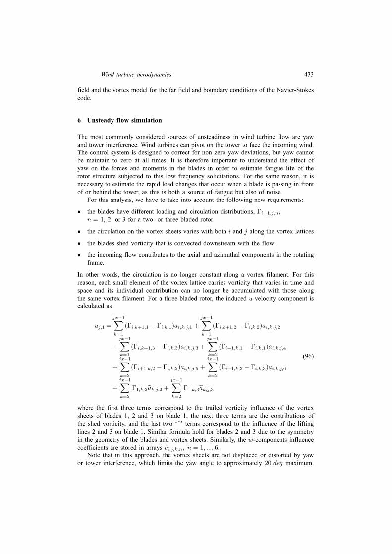
In other words, the circulation is no longer constant along a vortex filament. For thisreason, each small element of the vortex lattice carries vorticity that varies in time andspace and its individual contribution can no longer be accumulated with those alongthe same vortex filament. For a three-bladed rotor, the induced u-velocity component iscalculated as

uj,1 =

jx−1∑k=1

(Γi,k+1,1 − Γi,k,1)ai,k,j,1 +

jx−1∑k=1

(Γi,k+1,2 − Γi,k,2)ai,k,j,2

+

jx−1∑k=1

(Γi,k+1,3 − Γi,k,3)ai,k,j,3 +

jx−1∑k=2

(Γi+1,k,1 − Γi,k,1)ai,k,j,4

+

jx−1∑k=2

(Γi+1,k,2 − Γi,k,2)ai,k,j,5 +

jx−1∑k=2

(Γi+1,k,3 − Γi,k,3)ai,k,j,6

+

jx−1∑k=2

Γ1,k,2ak,j,2 +

jx−1∑k=2

Γ1,k,3ak,j,3

(96)

where the first three terms correspond to the trailed vorticity influence of the vortexsheets of blades 1, 2 and 3 on blade 1, the next three terms are the contributions ofthe shed vorticity, and the last two ‘˜’ terms correspond to the influence of the liftinglines 2 and 3 on blade 1. Similar formula hold for blades 2 and 3 due to the symmetryin the geometry of the blades and vortex sheets. Similarly, the w-components influencecoefficients are stored in arrays ci,j,k,n, n = 1, ..., 6.

Note that in this approach, the vortex sheets are not displaced or distorted by yawor tower interference, which limits the yaw angle to approximately 20 deg maximum.

434 J-J. Chattot

The vortex sheet is that which corresponds to zero yaw and no tower modelisation andis called the ‘base helix’. It is depicted in Figure 17.

One of the nice features of this approach is that the flow becomes periodic shortlyafter the initial shed vorticity has crossed the Trefftz plane, that is for a dimensionlesstime T ≥ xix

(1+2u) or a number of iterations n ≥ xix

(1+2u)∆t =xix

∆x .

6.1 Effect of Yaw

The procedure to calculate the circulation at the blades is unchanged. Once the inducedvelocities are obtained, the local incidence of the blade is found and the steady viscouspolar searched for lift and drag. The local blade element working conditions now dependon the yaw angle β and the azimuthal angle ψ measured to be zero when blade 1 is inthe vertical position. The lift provides the circulation according to the Kutta-Joukowskilift theorem

Γ1,j,1 =1

2qj,1cjCl j,1 (97)

where qj,1 is the local velocity magnitude, cj the chord and Cl j,1 the local liftcoefficient for blade 1.

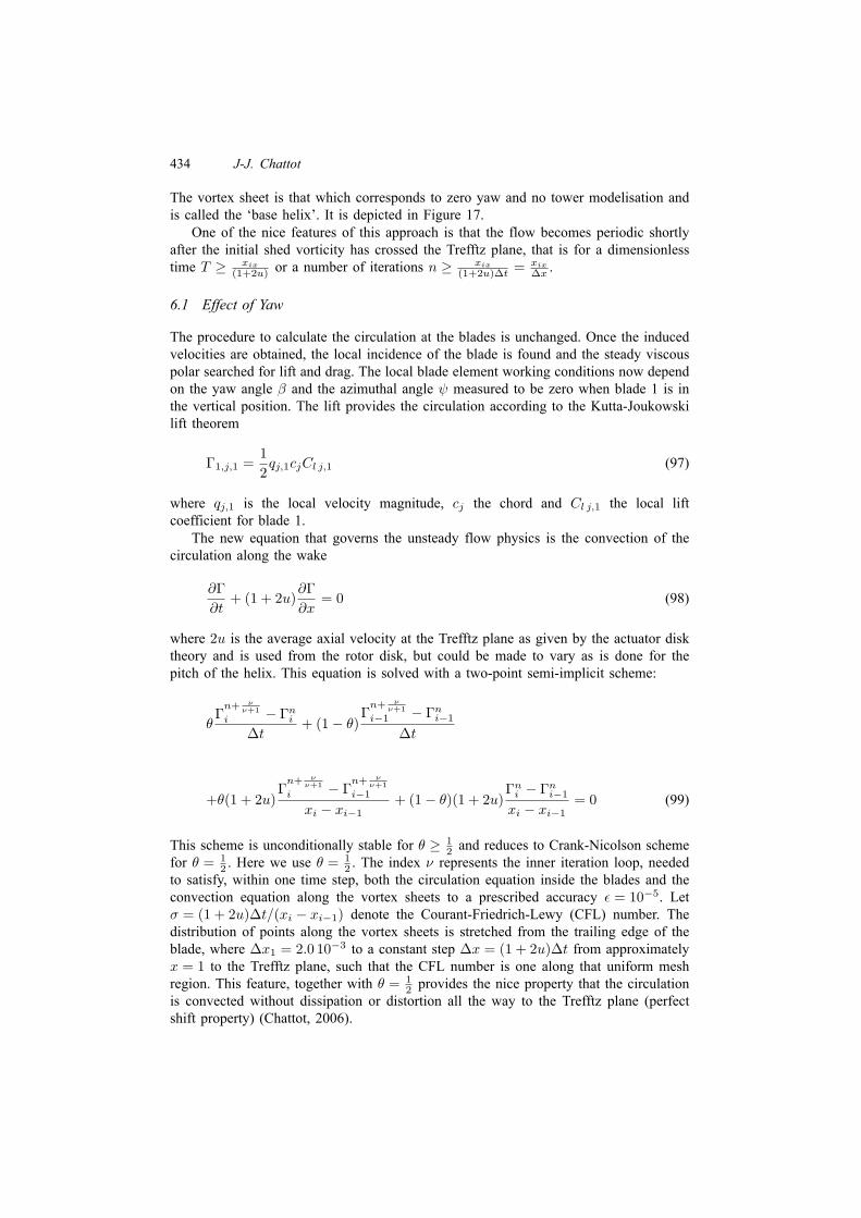
The new equation that governs the unsteady flow physics is the convection of thecirculation along the wake

∂Γ

∂t+ (1 + 2u)

∂Γ

∂x= 0 (98)

where 2u is the average axial velocity at the Trefftz plane as given by the actuator disktheory and is used from the rotor disk, but could be made to vary as is done for thepitch of the helix. This equation is solved with a two-point semi-implicit scheme:

θΓn+ ν

ν+1

i − Γni

∆t+ (1− θ)

Γn+ ν

ν+1

i−1 − Γni−1

∆t

+θ(1 + 2u)Γn+ ν

ν+1

i − Γn+ ν

ν+1

i−1

xi − xi−1+ (1− θ)(1 + 2u)

Γni − Γn

i−1

xi − xi−1= 0 (99)

This scheme is unconditionally stable for θ ≥ 12 and reduces to Crank-Nicolson scheme

for θ = 12 . Here we use θ =

12 . The index ν represents the inner iteration loop, needed

to satisfy, within one time step, both the circulation equation inside the blades and theconvection equation along the vortex sheets to a prescribed accuracy ϵ = 10−5. Letσ = (1 + 2u)∆t/(xi − xi−1) denote the Courant-Friedrich-Lewy (CFL) number. Thedistribution of points along the vortex sheets is stretched from the trailing edge of theblade, where ∆x1 = 2.0 10−3 to a constant step ∆x = (1 + 2u)∆t from approximatelyx = 1 to the Trefftz plane, such that the CFL number is one along that uniform meshregion. This feature, together with θ = 1

2 provides the nice property that the circulationis convected without dissipation or distortion all the way to the Trefftz plane (perfectshift property) (Chattot, 2006).


6.2 Tower interference model

Two configurations are considered in this section, one in which the rotor is upstream ofthe tower and the other in which it is downwind of the tower. These situations are quitedifferent from a physical point of view. In the former, the inviscid model is appropriateand the tower interference consists in a blockage effect due to the flow slowing downand stagnating along the tower. In the latter, the blade crosses the viscous wake of thetower, a region of rotational flow with low stagnation pressure, the extent of which aswell as steadiness characteristics depend on Reynolds number.

In the upwind configuration, the tower interference is modeled as a semi-infinite lineof doublets aligned with the incoming flow. One can show that the velocity potentialfor such a flow is given by

Φ(X,Y, Z) =V r2

2

X

X2 + Y 2

(1− Z√

X2 + Y 2 + Z2

)(100)

where r = r/R is the dimensionless tower radius. The coordinate system is alignedwith the wind, the X-axis being aligned and in the direction of the incoming flow, theZ-axis being vertical oriented upward and the Y -axis completing the direct orthonormalreference system (see Figure 17).

Figure 17 Displaced helix, base helix and coordinate system for the treatment of unsteady flows

VcosΒ

VsinΒV®

x

y

z

W

Β

base helix

displacedhelix

0

V cosΒ

V sinΒ

V®

x

X

y

Y

z

Z

Ψ

Β

In the downwind configuration, an empirical model due to Coton et Al. (2002) is used.The above potential model of the tower is applied almost everywhere, but when a bladeenters the narrow region |Y | ≤ 2.5 r corresponding to the tower shadow, the towerinduced axial velocity is set to ΦX = −0.3V and the other two components are set tozero.

The velocity field induced by the tower is given by ∇Φ = (ΦX ,ΦY ,ΦZ). In therotating frame, a point on blade 1 has coordinates (0, yj , 0). Let d = d/R be thedimensionless distance of the rotor from the tower axis. A negative value indicatesupwind configuration, while a positive value indicates downwind case. In the fixedframe of reference, such a point has coordinates given by

436 J-J. ChattotXYZ

=

cosβ − sinβ 0sinβ cosβ 00 0 1

dyj sinψyj cosψ

(101)

Using the same transformation, the tower-induced velocities at the blade can becalculated with the help of the components of the unit vectors in the rotating frame:

−→i−→j−→k

=

cosβ sinβ 0− sinβ sinψ cosβ sinψ cosψsinβ cosψ − cosβ cosψ sinψ

−→I−→J−→K

(102)

where (−→i ,

−→j ,

−→k ) and (

−→I ,

−→J ,

−→K) are the unit vectors in the rotating frame and

the wind frame respectively. For blade 1 the induced velocities are uj,1 = (∇Φ.−→i )

and wj,1 = (∇Φ.−→k ). Application of this formula to the incoming flow

−→V = (1, 0, 0)

provides the axial and azimuthal components of the unperturbed flow in the rotatingframe, again for blade 1

u = (−→V .

−→i ) = cosβ (103)

w = (−→V .

−→k ) = sinβ cosψ (104)

6.3 Validation

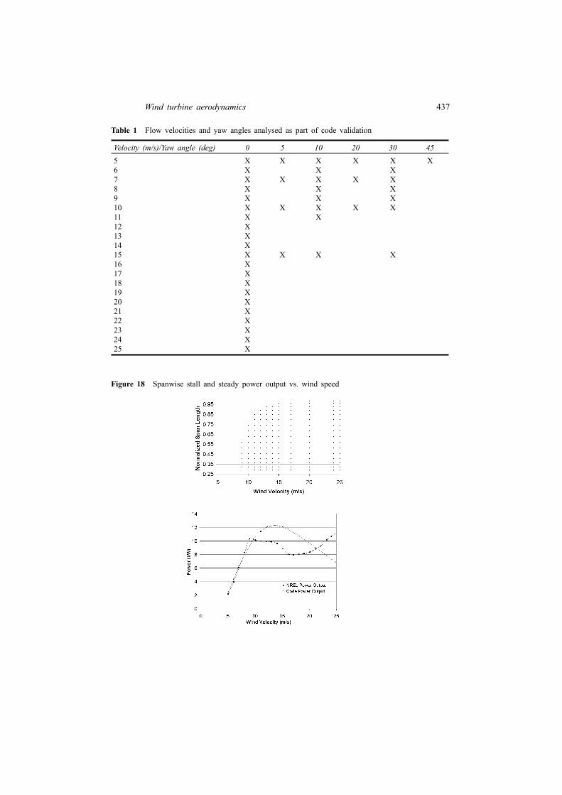
The helicoidal vortex model has been applied to a large number of cases, steady andunsteady, from the two-bladed rotor NREL S data sequence, in order to explore thedomain of validity and assess the accuracy of this approach (Hallissy and Chattot, 2005),see Table 1. In the experiments, the rotation speed of the turbine was held constant at72 rpm, thus velocity was the main control parameter to vary the TSR. As velocityincreases and TSR decreases, stall affects a larger and larger part of the blades. Insteady flow conditions (β = 0), incipient separation occurs around 8 m/s and thenspreads to the whole blade above 15 m/s. This is shown in Figure 18 where the topgraph indicates with dots the points along the blade where stall occurs. The bottom plotshows the steady power output comparison with the experimental data.

As can be seen, the agreement with the power output is excellent until V = 8 m/s,that is until there is separated flow on the blades.

The effect of yaw on power is analysed. The flow at yaw is periodic and the averagepower is calculated and compared with the average power given in the NREL database.The results are shown in Figure 19. Good results are obtained with the vortex modelfor yaw angles of up to β = 20 deg. This is consistent with the approximate treatmentof the vortex sheets.


Table 1 Flow velocities and yaw angles analysed as part of code validation

Velocity (m/s)/Yaw angle (deg) 0 5 10 20 30 455 X X X X X X6 X X X7 X X X X X8 X X X9 X X X10 X X X X X11 X X12 X13 X14 X15 X X X X16 X17 X18 X19 X20 X21 X22 X23 X24 X25 X

Figure 18 Spanwise stall and steady power output vs. wind speed

438 J-J. Chattot

Figure 19 Average power output vs. wind speed at β = 5, 10, 20 and 30 deg


7 Hybrid method

Euler and Navier-Stokes solvers employ dissipative schemes to ensure the stabilityof the computation, either built into the numerical scheme or added artificially as asupplemental viscosity term. The dissipative property of those schemes works well withdiscontinuities such as shock waves, but has an adverse effect on discontinuities suchas contact discontinuities and vortex sheets. It has been known for a long time thatthese schemes dissipate contact discontinuities associated with the shock-tube problemand vortex sheets trailing a finite wing, helicopter rotor, propeller and wind turbine.In the case of turbine flow, the influence of the vortex sheets is rapidly lost, whichhas an effect on the blade working conditions by not accounting for induced velocitiescontributed by the lost part of the wake.

On the other hand, the vortex model described earlier can maintain the vortex sheetsas far downstream as needed, but cannot handle large span-wise gradients resulting inparticular from viscous effects and separation.

In the rest of this section, we will present some results of the hybrid method whichconsists in coupling a Navier-Stokes solver with the vortex model, the former beinglimited to a small region surrounding the blades where the more complex physics canbe well represented, and the latter being responsible to carry the circulation to the farfield and impress on the Navier-Stokes’ domain outer boundary the induced velocitiesaccurately calculated by the Biot-Savart law. This new approach has been found to beboth more accurate and more efficient than full domain Navier-Stokes calculations, bycombining the best capabilities of the two models.

Figure 20 Coupling methodology (see online version for colours)

The coupling procedure is described in Figure 20. It consists in calculating theNavier-Stokes solution with boundary conditions that only account for incoming flowand rotating frame relative velocities at the outer boundary of the domain. Thesolution obtained provides, by path integration, the circulation at each vortex location

440 J-J. Chattot

along the trailing edge of the blade and the Biot-Savart law allows to update thevelocity components at the outer boundary of the Navier-Stokes region by adding thewake-induced contributions. This closes the iteration loop with a new Navier-Stokessolution. It takes approximately five cycles for the circulation to be converged with|∆Γ| < 10−5.

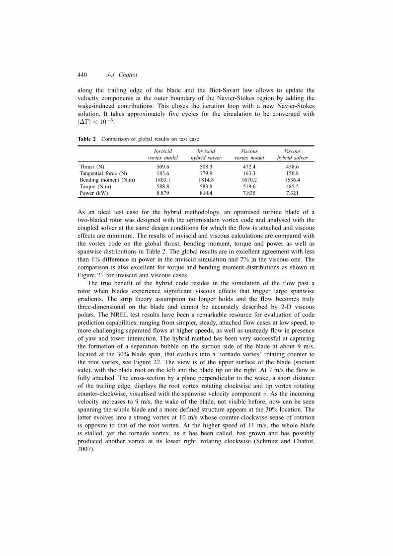
Table 2 Comparison of global results on test case

Inviscid Inviscid Viscous Viscousvortex model hybrid solver vortex model hybrid solver

Thrust (N) 509.6 508.3 472.4 458.6Tangential force (N) 183.6 179.9 163.3 150.8Bending moment (N.m) 1803.1 1814.8 1670.2 1636.4Torque (N.m) 588.8 583.8 519.6 485.5Power (kW) 8.879 8.804 7.835 7.321

As an ideal test case for the hybrid methodology, an optimised turbine blade of atwo-bladed rotor was designed with the optimisation vortex code and analysed with thecoupled solver at the same design conditions for which the flow is attached and viscouseffects are minimum. The results of inviscid and viscous calculations are compared withthe vortex code on the global thrust, bending moment, torque and power as well asspanwise distributions in Table 2. The global results are in excellent agreement with lessthan 1% difference in power in the inviscid simulation and 7% in the viscous one. Thecomparison is also excellent for torque and bending moment distributions as shown inFigure 21 for inviscid and viscous cases.

The true benefit of the hybrid code resides in the simulation of the flow past arotor when blades experience significant viscous effects that trigger large spanwisegradients. The strip theory assumption no longer holds and the flow becomes trulythree-dimensional on the blade and cannot be accurately described by 2-D viscouspolars. The NREL test results have been a remarkable resource for evaluation of codeprediction capabilities, ranging from simpler, steady, attached flow cases at low speed, tomore challenging separated flows at higher speeds, as well as unsteady flow in presenceof yaw and tower interaction. The hybrid method has been very successful at capturingthe formation of a separation bubble on the suction side of the blade at about 9 m/s,located at the 30% blade span, that evolves into a ‘tornado vortex’ rotating counter tothe root vortex, see Figure 22. The view is of the upper surface of the blade (suctionside), with the blade root on the left and the blade tip on the right. At 7 m/s the flow isfully attached. The cross-section by a plane perpendicular to the wake, a short distanceof the trailing edge, displays the root vortex rotating clockwise and tip vortex rotatingcounter-clockwise, visualised with the spanwise velocity component v. As the incomingvelocity increases to 9 m/s, the wake of the blade, not visible before, now can be seenspanning the whole blade and a more defined structure appears at the 30% location. Thelatter evolves into a strong vortex at 10 m/s whose counter-clockwise sense of rotationis opposite to that of the root vortex. At the higher speed of 11 m/s, the whole bladeis stalled, yet the tornado vortex, as it has been called, has grown and has possiblyproduced another vortex at its lower right, rotating clockwise (Schmitz and Chattot,2007).


Figure 21 Vortex model (VLM) and hybrid code (PCS) comparison: (a) inviscid and(b) viscous torque and bending moment distributions

0.2 0.3 0.4 0.5 0.6 0.7 0.8 0.9 1−40

−20

0

20

40

60

80

100

120

r / R

Mom

ent [

N/m

* m

]Bending (VLM)Bending (PCS)Torque (VLM)Torque (PCS)

(a)

0.2 0.3 0.4 0.5 0.6 0.7 0.8 0.9 1−40

−20

0

20

40

60

80

100

r / R

Mom

ent [

N/m

* m

]

Bending (VLM)Bending (PCS)Torque (VLM)Torque (PCS)

(b)

8 Perspectives

The design of blades is still a major task for manufacturers. Aerodynamics andstructures are intimately associated in this process, to account for fabrication cost,transportation/installation, maintenance and fatigue life. Steady flow modelisationremains the primary preoccupation of the designers, while unsteady effects contribute tothe overall system performance assessment.

442 J-J. Chattot

The importance of unsteadiness and its modelisation in wind turbine aerodynamics isgreater than ever before, in large part due to the larger size of the blades and their greater‘softness’ or flexibility. Advanced designs are contemplated that incorporate blade sweepand winglets with a view to improving the performance and power capture (Chattot,2008). Composite materials allow for these increases in size and complexity, but alsodecreased stiffness. The question of fatigue has therefore become more relevant as theblades are subject to more vibrations, bending and twisting.

Figure 22 Development of a well-defined viscous feature above the NREL blade (a) V = 7 m/s(b) V = 9 m/s (c) V = 10 m/s (d) V = 11 m/s (see online version for colours)

(a)

(b)


Figure 22 Development of a well-defined viscous feature above the NREL blade(a) V = 7 m/s (b) V = 9 m/s (c) V = 10 m/s (d) V = 11 m/s (continued)(see online version for colours)

(c)

(d)

The vortex model has the potential of providing useful capabilities for the simulationof aeroelastic phenomena. Some work has already been carried out in this direction(Chattot, 2007). More work needs to be done to obtain a realistic simulation tool thatis cheap and reliable, and operates directly in the time domain, in contrast to the manyapproaches based on eigen-frequencies and eigen-modes in the frequency domain withhighly simplified aerodynamics. The hybrid method would be a natural candidate forthe extension to fluid/structure interaction when viscous effects are important.

444 J-J. Chattot

ReferencesBetz, A. (1919) Schraubenpropeller mit geringstem Energieverlust, Nach der Kgl. Gesellschaft

der Wiss. zu Gottingen, Math.-Phys. Klasse, pp.193–217; reprinted in Vier Abhandlungen zurHydro- und Aero-dynamik, by L. Prandtl and A. Betz (Eds.), Gottingen, 1927 (reprint Ann Arbor:Edwards Bros. 1943), pp.68–92.

Betz, A. (1926) Wind Energie und Ihre Ausnutzung durch Windmuhlen, Gottingen, Vandenhoeck.Chattot, J-J. (2003) ‘Optimization of wind turbines using helicoidal vortex model’, Journal of Solar

Energy Engineering, Special Issue: Wind Energy, Vol. 125, No. 4, pp.418–424.Chattot, J-J. (2004a) Computational Aerodynamics and Fluid Dynamics: An Introduction, Springer

Verlag, Scientific Computation, ISBN 3-540-43494-1, Second Printing.Chattot, J-J. (2004b) ‘Analysis and design of wings and wing/winglet combinations at low speeds’,

Computational Fluid Dynamics Journal, Special Issue, Vol. 13, No. 3.Chattot, J-J. (2006) ‘Helicoidal vortex model for steady and unsteady flows’, Computers and Fluids,

Vol. 35, pp.733–741.Chattot, J-J. (2007) ‘Helicoidal vortex model for wind turbine aeroelastic simulation’, Computers and

Structures, Vol. 85, pp.1072–1079.Chattot, J-J. (2008) ‘Effects of blade tip modifications on wind turbine performance using vortex

model’, Computers and Fluids, Vol. 38, No. 7, pp.1405–1410.Coton, F.N., Wang, T., Galbraith, R.A.M. (2002) ‘An examination of key aerodynamics modeling

issues raised by the NREL blind comparison’, AIAA Paper No. 0038.Drela, M. (1989) ‘XFOIL: an analysis and design system for low Reynolds number airfoils’, in

T.J. Mueller (Eds.): Lecture Notes in Engineering, pp.1–12, No. 54, Low Reynolds NumberAerodynamics, Springer-Verlag, Berlin.

Froude, R.E. (1889) Transactions, Institute of Naval Architects, Vol. 30, p.390.Goldstein, S. (1929) ‘On the vortex theory of screw propellers’, Proceedings of the Royal Society of

London, Series A, Vol. 123, pp.440–465.Hallissy, J.M. and Chattot, J-J. (2005) ‘Validation of a helicoidal vortex model with the NREL

unsteady aerodynamic experiment’, Computational Fluid Dynamics Journal, Special Issue,Vol. 14, No. 3, pp.236–245.

Hand, M.M., Simms, D.A., Fingersh, L.J., Jager, D.W., Cotrell, J.R., Schreck, S. and Larwood, S.M.,(2001) Unsteady Aerodynamics Experiment Phase VI: Wind Tunnel Test Configurations andAvailable Data Campaigns, NREL/TP-500-29955.

Joukowski, N.E. (1918) Travaux du Bureau des Calculs et Essais Aeronautiques de l’Ecole SuperieureTechnique de Moscou.

Munk, M.M. (1921) The Minimum Induced Drag of Aerofoils, NACA Rept. 121.Prandtl, L. and Betz, A. (1927)Vier Abhandlungen zur Hydro- und Aero-dynamik, Selbstverlag des

Kaiser Wilhelminstituts fur Stromungsforshung, Gottingen Nachr., Gottingen, Germany.Rankine, W.J. (1865) Transactions, Institute of Naval Architects, Vol. 6, p.13.Schmitz, S. and Chattot, J-J. (2007) ‘Method for aerodynamic analysis of wind turbines at peak

power’, Journal of Propulsion and Power, Vol. 23, No. 1, pp.243–246.

jean-jacques chattotmae.engr.ucdavis.edu/chattot/publications/ijad0103-0410_chattot.pdf ·...

Documents