j. martinec, a. rango, r. roberts snowmelt runoff...

Snowmelt Runoff Model (SRM) User’s Manual

Edited by Enrique Gómez-Landesa & Max P. Bleiweiss

J. Martinec, A. Rango, R. Roberts

Agricultural Experiment Station • Special Report 100College of Agriculture and Home Economics

WINDOWS PROGRAM FOR

IMPROVED RUNOFF FORECASTS

AND EFFECT OF CLIMATE CHANGE

Acknowledgment

It has taken the efforts of many people and the support of their organization during the last several years to allow us to reach this new milestone in snowmelt runoff modeling. The following organizations and people were particularly helpful and supportive:

USDA/ARS Jornada Experimental Range, Las Cruces, NMUSDA/ARS Hydrology and Remote Sensing Laboratory, Beltsville, MDBureau of Reclamation—El Paso, TX (Mr. Michael Landis)Rio Grande Basin Initiative, New Mexico State University, Las Cruces, NMNMSU Water Task Force, New Mexico State University, Las Cruces, NM (Mr. Craig Runyan)US Army Corps of Engineers—Albuquerque, NM (Ms. Gail Stockton)US Army Research Laboratory—WSMR, NMMcElyea Family Endowment for Water Research

S R M

SNOWMELT RUNOFF MODEL

USER’S MANUAL

UPDATED EDITION FOR WINDOWS

WinSRM Version 1.11 February, 2008

Jaroslav Martinec, Albert Rango & Ralph Roberts

Edited by Enrique Gómez-Landesa & Max P. Bleiweiss

2

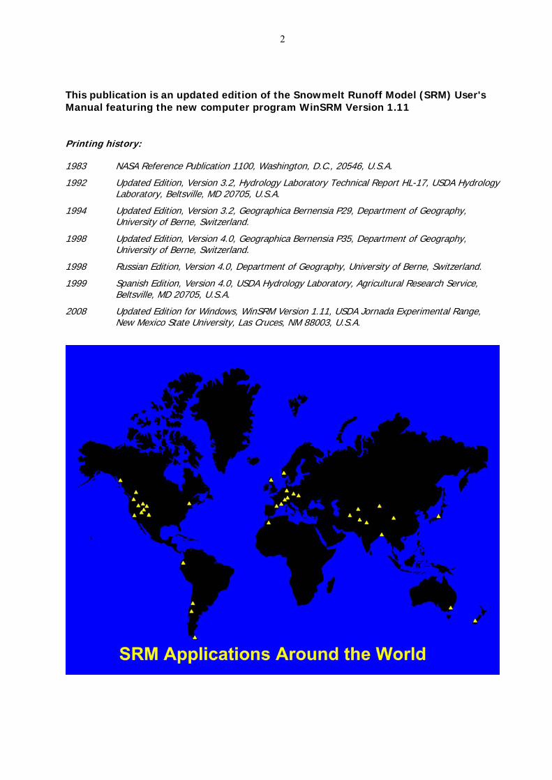
This publication is an updated edition of the Snowmelt Runoff Model (SRM) User's Manual featuring the new computer program WinSRM Version 1.11 Printing history: 1983 NASA Reference Publication 1100, Washington, D.C., 20546, U.S.A.

1992 Updated Edition, Version 3.2, Hydrology Laboratory Technical Report HL-17, USDA Hydrology Laboratory, Beltsville, MD 20705, U.S.A.

1994 Updated Edition, Version 3.2, Geographica Bernensia P29, Department of Geography, University of Berne, Switzerland.

1998 Updated Edition, Version 4.0, Geographica Bernensia P35, Department of Geography, University of Berne, Switzerland.

1998 Russian Edition, Version 4.0, Department of Geography, University of Berne, Switzerland.

1999 Spanish Edition, Version 4.0, USDA Hydrology Laboratory, Agricultural Research Service, Beltsville, MD 20705, U.S.A.

2008 Updated Edition for Windows, WinSRM Version 1.11, USDA Jornada Experimental Range, New Mexico State University, Las Cruces, NM 88003, U.S.A.

3

SNOWMELT RUNOFF MODEL (SRM)

USER'S MANUAL

(Updated Edition 2008, Windows Version 1.11)

J. Martinec Consulting Hydrologist

Davos, Switzerland

A. Rango Jornada Experimental Range

USDA-Agricultural Research Service (ARS) Las Cruces, New Mexico, USA

R. Roberts Hydrology & Remote Sensing Laboratory

USDA-ARS Beltsville, Maryland, USA

Edited by

E. Gómez-Landesa M. P. Bleiweiss

New Mexico State University Las Cruces, New Mexico, USA

4

Contents

1 PREFACE ...................................................................................................................................13

2 INTRODUCTION ..........................................................................................................................13

3 RANGE OF CONDITIONS FOR MODEL APPLICATION ......................................................................14

4 MODEL STRUCTURE ....................................................................................................................19

5 NECESSARY DATA FOR RUNNING THE MODEL ..............................................................................21

5.1 Basin characteristics ......................................................................................................21 5.1.1 Basin and zone areas .....................................................................................21 5.1.2 Area-elevation curve ......................................................................................22

5.2 Variables ......................................................................................................................23 5.2.1 Temperature and degree-days, T ....................................................................23 5.2.2 Precipitation, P ..............................................................................................24 5.2.3 Snow covered area, S ....................................................................................25

5.3 Parameters ...................................................................................................................29 5.3.1 Runoff coefficient, c .......................................................................................29 5.3.2 Degree-day factor, a ......................................................................................31 5.3.3 Temperature lapse rate, γ...............................................................................32 5.3.4 Critical temperature, TCRIT...............................................................................33 5.3.5 Rainfall contributing area, RCA........................................................................33 5.3.6 Recession coefficient, k ..................................................................................34 5.3.7 Time Lag, L ...................................................................................................40

6 ASSESSMENT OF THE MODEL ACCURACY......................................................................................42

6.1 Accuracy criteria............................................................................................................42 6.1.1 Accuracy criteria in model tests.......................................................................44 6.1.2 Model accuracy outside the snowmelt season...................................................46

6.2 Elimination of possible errors..........................................................................................46

7 OPERATION OF THE MODEL FOR REAL TIME FORECASTS ..............................................................50

7.1 Extrapolation of the snow coverage ................................................................................50 7.2 Updating ......................................................................................................................55

8 YEAR-ROUND RUNOFF SIMULATION FOR A CHANGED CLIMATE .....................................................57

8.1 Snowmelt runoff computation in the winter half year........................................................57 8.2 Change of snow accumulation in the new climate ............................................................59 8.3 Runoff simulation for scenarios of the future climate ........................................................61 8.4 Model parameters in a changed climate ..........................................................................69 8.5 Normalization of data to represent the present climate.....................................................70 8.6 WinSRM to improve real time runoff forecasts .................................................................77

5

9 RUNOFF MODELING IN GLACIERIZED BASINS ...............................................................................78

9.1 Runoff increase in a warmer climate from glacier melt......................................................78 9.2 Long term behavior of glaciers in a warming climate ........................................................82

10 SRM FOR WINDOWS (WINSRM) COMPUTER PROGRAM...............................................................83

10.1 Program overview .......................................................................................................83 10.1.1 Historical background ...................................................................................83 10.1.2 Program description .....................................................................................84 10.1.3 Capabilities and limitations............................................................................85

10.2 WinSRM user interface.................................................................................................85 10.2.1 Entry window features..................................................................................85

10.3 WinSRM window descriptions .......................................................................................87 10.3.1 Welcome to WinSRM window ........................................................................87

10.3.1.1 Purpose..............................................................................................87 10.3.1.2 Buttons ..............................................................................................87

10.3.2 WinSRM main window ..................................................................................88 10.3.2.1 Purpose..............................................................................................88 10.3.2.2 Menu .................................................................................................88 10.3.2.3 Buttons ..............................................................................................93 10.3.2.4 Basin definition frame..........................................................................94 10.3.2.5 Basin simulation frame.........................................................................94 10.3.2.6 Status bar...........................................................................................95

10.3.3 Edit simulation control information window ....................................................95 10.3.3.1 Method of access ................................................................................95 10.3.3.2 Purpose..............................................................................................96 10.3.3.3 Buttons ..............................................................................................96

10.3.4 Edit {type of data} window...........................................................................96 10.3.4.1 Method of access ................................................................................96 10.3.4.2 Purpose..............................................................................................97 10.3.4.3 Data selection / data entry...................................................................97 10.3.4.4 Buttons ..............................................................................................98

10.3.5 Climate change scenario definition window.....................................................99 10.3.5.1 Method of access ................................................................................99 10.3.5.2 Purpose..............................................................................................99 10.3.5.3 Data entry and selection ....................................................................100 10.3.5.4 Buttons ............................................................................................100

10.3.6 Simulation statistics window........................................................................101 10.3.6.1 Method of access ..............................................................................101 10.3.6.2 Purpose............................................................................................101 10.3.6.3 Buttons ............................................................................................102

6

10.3.7 Run a climate change window.......................................................................102

10.3.7.1 Method of access ................................................................................102 10.3.7.2 Purpose..............................................................................................102 10.3.7.3 Buttons ..............................................................................................102 10.3.7.4 Processing steps controlled by the step buttons .....................................106

10.3.8 Long term monthly averages window.............................................................106 10.3.8.1 Method of access ................................................................................106 10.3.8.2 Purpose..............................................................................................107

10.3.9 Custom lag time distribution window .............................................................107 10.3.9.1 Method of access ................................................................................107 10.3.9.2 Purpose..............................................................................................107

10.3.10 Graphics window........................................................................................107 10.3.10.1 Method of access...............................................................................107 10.3.10.2 Purpose ............................................................................................108 10.3.10.3 Button-bar menu ...............................................................................109

10.3.11 Line attributes window................................................................................110 10.3.11.1 Method of access...............................................................................110 10.3.11.2 Purpose ............................................................................................110 10.3.11.3 Buttons.............................................................................................111

10.3.12 Output definition window............................................................................111 10.3.12.1 Method of access...............................................................................111 10.3.12.2 Purpose ............................................................................................111 10.3.12.3 Buttons.............................................................................................112 10.3.12.4 Available reports................................................................................112

10.3.13 File display window ....................................................................................113 10.3.13.1 Method of access...............................................................................113 10.3.13.2 Purpose ............................................................................................113 10.3.13.3 Menu................................................................................................113 10.3.13.4 Window control ................................................................................114

10.4 WinSRM operation.......................................................................................................114 10.4.1 Building a WinSRM basin database ................................................................114

10.4.1.1 Manually populate your WinSRM database.............................................114 10.4.1.2 Import an existing DOS .SRM data file...................................................116

10.4.2 Data base data entry....................................................................................117 10.4.3 Running WinSRM .........................................................................................117

10.4.3.1 WinSRM processing steps.....................................................................117

11. REFERENCES............................................................................................................................118

11.1 General references ......................................................................................................118 11.2 Specific references for Table 1......................................................................................121

7

Appendix A – Examples...................................................................................................................128

Example 1 – Create a new basin database by importing a DOS .SRM data file..........................128 Example 2 – Adding physical data to a database from another (digital) source.........................129 Example 3 – Developing a climate change scenario................................................................130 Example 4 – Simulating climatechange using a climate change scenario ..................................131 Example 5 – Developing a custom climate change scenario ....................................................132 Example 6 – Developing a normalized year ...........................................................................134

Appendix B – Graphical Plots ...........................................................................................................138

Appendix C – Program Windows ......................................................................................................139

Appendix D – WinSRM Database Schema .........................................................................................140

BasinDescription Table ........................................................................................................140 ZoneDescription Table.........................................................................................................140 SimulationIndex Table.........................................................................................................141 PhysicalData Table..............................................................................................................142 Simulation Parameter Table .................................................................................................143 SimResults Table ................................................................................................................144 ClimateScenarioIndex Table.................................................................................................146 ClimateScenario Table.........................................................................................................147

Appendix E – Additional Windows ....................................................................................................148

Appendix F – Program Message Dialogs ...........................................................................................149

Appendix G – SRM Computer Program Version 4...............................................................................150

G.1 Background.................................................................................................................150 G.2 Getting started ............................................................................................................150

G.2.1 System requirements .....................................................................................150 G.2.2 Installing Micro-SRM......................................................................................150 G.2.3 Configuring Micro-SRM...................................................................................151 G.2.4 Operating instructions....................................................................................151

G.3 Program features.........................................................................................................152 G.3.1 Screen display types ......................................................................................152 G.3.2 Text screens .................................................................................................153 G.3.3 Menu screens................................................................................................153 G.3.4 Data entry screens ........................................................................................154 G.3.5 Program options............................................................................................156 G.3.6 Basin definition .............................................................................................156 G.3.7 Basin variables/parameters ............................................................................156 G.3.8 Climate change processing control screens ......................................................157

G.3.8.1 Climate change control screen ..............................................................157 G.3.8.2 Climate change progress screen............................................................158

G.4 Keyboard definition ......................................................................................................161 G.4.1 Global definitions...........................................................................................161 G.4.2 Cursor movement keys ..................................................................................162 G.4.3 Field editing keys...........................................................................................162

8

G.4.4 Function keys................................................................................................163 G.4.5 Alternate function keys ..................................................................................166

G.5 Micro-SRM output products...........................................................................................167 G.5.1 Simulation/forecast statistics ..........................................................................167 G.5.2 Summary display...........................................................................................167 G.5.3 .SRM data file ...............................................................................................167 G.5.4 Plot displays..................................................................................................167

G.5.4.1 Plot displays (climate change)...............................................................168 G.5.5 Printed reports ..............................................................................................168 G.5.6 Printed reports (climate change).....................................................................169

G.6 Using Micro-SRM..........................................................................................................170 G.7 Using Micro-SRM to simulate a year-round climate change ..............................................171 G.8 Using Micro-SRM trace file options ................................................................................174 G.9 Micro-SRM availability ..................................................................................................175

List of Figures Figure 1. Selected locations where SRM has been tested. ............................................................... 13

Figure 2. Elevation zones and areas of the South Fork of the Rio Grande basin, Colorado, USA. .......... 21

Figure 3. Determination of zonal mean hypsometric elevations (h ) using an area-elevation curve for the

South Fork of the Rio Grande basin. ..................................................................................... 22

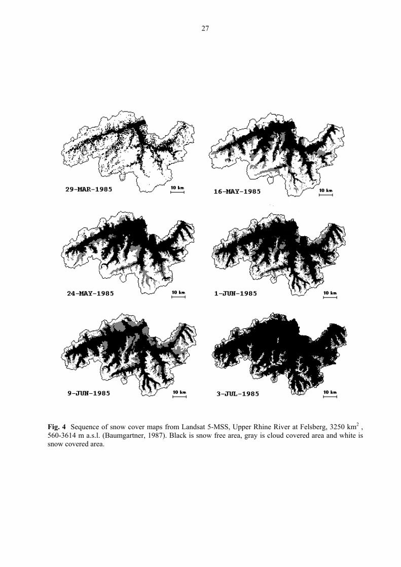
Figure 4. Sequence of snow cover maps from Landsat 5-MSS, Upper Rhine River at Felsberg, 3250 km2,

560-3614 m a.s.l. (Baumgartner, 1987). ............................................................................... 27

Figure 5. Example of a possible distortion of a depletion curve due to a temporary increase in the snow

coverage by a summer snowfall and to missing Landsat data from the preceding overflight (Hall &

Martinec, 1985). . ................................................................................................................ 28

Figure 6. Depletion curves of the snow coverage for 5 elevation zones of the basin Felsberg, derived from

the Landsat imagery shown in Figure 4 (Baumgartner, 1987). ................................................ 28

Figure 7. Average runoff coefficient for snow (cs) for the alpine basins Dischma (43.3 km2, 1668-3146 m

a.s.l.) and Durance (2170 km2, 786-4105 m a.s.l.) (Martinec & Rango, 1986). ......................... 31

Figure 8. Average runoff coefficient for rainfall (cR) for the basins Dischma and Durance (Martinec &

Rango, 1986). .................................................................................................................... 31

Figure 9. Average degree-day ratio (a) used in runoff simulations by the SRM model in the basins

Dischma (10 years), Durance (5 years) and Dinwoody (228 km2; 1981-4202 m a.s.l., Wyoming, 2

years) (Martinec & Rango, 1986). ......................................................................................... 33

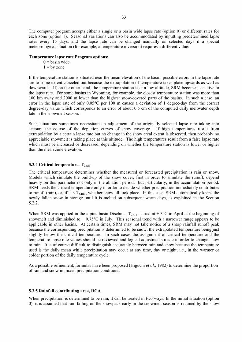
Figure 10. Recession flow plot Qn vs Qn+1 for the Dischma basin in Switzerland. Either the solid envelope

line or the dashed medium line is used to determine k-values for computing the constants x and y

in Equation (7) (Martinec & Rango, 1986). ............................................................................ 35

Figure 11. Range of recession coefficients, k, related to discharge Q resulting from various evaluations

(Martinec & Rango, 1986). ................................................................................................... 36

9

Figure 12. Snowmelt hydrographs illustrating the conversion of computed runoff amounts for 24 hour

perioids to calendar day periods (Martinec & Rango, 1986). ...................................................40

Figure 13. Runoff simulations in the basin of the Rio Grande near Del Norte, Colorado (3419 km2, 2432-

4215 m a.s.l.) (Martinec & Rango, 1989). ............................................................................. 43

Figure 14. Combined representation of model performances for average inaccuracies using three criteria:

R2, DG and Dv (Rango and Martinec, 1988). .......................................................................... 45

Figure 15. Combined representation of model performances for maximum inaccuracies using three

criteria: R2, DG and Dv (Rango and Martinec, 1988). .............................................................. 45

Figure 16. Runoff simulations in the basin Dischma (43.3 km2, 1668-3146 m a.s.l.) (Martinec & Rango,

1986). ................................................................................................................................ 46

Figure 17. Runoff simulation in the catchment area of the hydroelectric station Sedrun (Swiss Alps, 108

km2, 1840-3210 m a.s.l.) (Baumann et al., 1990). ................................................................. 50

Figure 18. Runoff simulation in the catchment area of the hydroelectric station Tavanasa (Swiss Alps, 215

km2, 1277-3210 m a.s.l.) (Baumann et al., 1990). ................................................................. 51

Figure 19. Extrapolation of snow cover depletion curves in real-time from modified depletion curves with

the use of temperature forecasts (Hall & Martinec, 1985). ...................................................... 52

Figure 20. Elimination of the effect of antecedent snowfall on the extrapolation of depletion curves of

snow coverage (Hall & Martinec, 1985). ................................................................................ 52

Figure 21. Nomograph of modified depletion curves for the elevation zone B (1284 km2, 2926-3353 m

a.s.l.) of the Rio Grande basin near Del Norte, Colorado. ........................................................ 54

Figure 22. Simulated real-time runoff forecast for the Rio Grande basin using long-term average

temperatures instead of temperatures for the year 1983 (Rango & van Katwijk, 1990). ............ 54

Figure 23. Real-time availability of temperature and precipitation data for short-term runoff forecasts in

contrast to runoff simulation. ............................................................................................... 55

Figure 24. Discharge simulation in the Dinwoody Creek basin (228 km2, 1981-4202 m a.s.l.) in Wyoming,

(a) without updating (b) with updating by actual discharge on 1 August. . ................................ 56

Figure 25. Illustration of the snow accumulation in the winter and snowmelt in the summer in the

present climate (hypothetical example). ................................................................................ 60

Figure 26. Illustration of the snow accumulation in the winter and snowmelt in the summer in a warmer

climate (hypothetical example). ............................................................................................ 61

Figure 27. Measured and simulated runoff in the Rio Grande basin near Del Norte, Colorado in the

hydrological year 1979. . ...................................................................................................... 63

Figure 28. Conventional depletion curves of the snow coverage from Landsat data in the elevation zones

A, B and C of the Rio Grande basin near Del Norte, Colorado in 1979. ..................................... 65

Figure 29. Modified depletion curves for zone A: MDCINCL derived from CDC, therefore including new

snow, MDCEXCL with new snowmelt excluded, MDCEXCL WA with "winter deficit" (shaded area)

cut off. ............................................................................................................................... 65

10

Figure 30. Accumulated zonal melt curves for zone A: AZMINCL computed daily melt depth multiplied by S

from CDC (= zonal melt). . ................................................................................................... 66

Figure 31. Modified depletion curve, adjusted for the "winter deficit" and including new snow of the

changed climate (MDCCLIM WA) derived from MDCEXCL WA for zone A. . ......................................... 66

Figure 32. Effect of a changed climate (T + 4ºC) on snow covered areas of 1979 in elevation zones A, B,

and C of the Rio Grande basin near Del Norte, Colorado. ........................................................ 67

Figure 33. Climate-affected runoff (T + 4ºC) in the Rio Grande basin near Del Norte, Colorado, compared

with the runoff simulate by data of 1979.(as shown in Figure 27) for April-September. ............. 67

Figure 34. Simulated runoff in the Rio Grande basin near Del Norte, Colorado, in the hydrological

year1979 and climate-affected runoff computed by increased temperatures (T + 4ºC) and

correspondingly changed snow conditions. ............................................................................ 68

Figure 35. Normalized depletion curves of the snow coverage (9979) in the Rio Grande basin near Del

Norte, Colorado (dashed lines) derived from the measured curves of 1979 (solid lines), zones A, B,

and C. ................................................................................................................................ 73

Figure 36. Normalized runoff (9979) derived from the runoff of 1979 by normalized temperatures and

precipitation, Rio Grande basin near Del Norte, Colorado. ....................................................... 73

Figure 37. Effect of a changed climate (T + 4ºC) on the normalized snow covered areas in elevation

zones A, B, and C of the Rio Grande basin near Del Norte, Colorado. ...................................... 74

Figure 38. Effect of a changed climate (T + 4ºC) on the normalized runoff (9979) in the Rio Grande basin

near Del Norte, Colorado. .................................................................................................... 74

Figure 39. Conventional depletion curves of the snow coverage (CDC's) in the Rio Grande basin near Del

Norte, Colorado in the years 1977 and 1979. ......................................................................... 75

Figure 40. Depletion curves of the snow coverage (CDC's) in the Rio Grande basin near Del Norte,

Colorado measured in 1979 and derived for 1977 by the climate program. .............................. 75

Figure 41. Transformation of runoff in the Rio Grande basin near Del Norte, Colorado from runoff in 1979

to runoff in 1977, using temperature and precipitation of 1977 as "new climate" for 1979. ........ 76

Figure 42. Measured and computed runoff in the Illecillewaet basin in the year 1984. ........................ 80

Figure 43. Measured and climate-affected (T + 4ºC) depletion curves of the snow coverage in all

elevation zones including the glacier zones C and D of the Illecillewaet basin. .......................... 80

Figure 44. Computed runoff in the Illecillewaet basin in the year 1984 and climate-affected runoff

increased by glacier melt. .................................................................................................... 81

Figure 45. Objects of the Graphical User Interface (GUI) window. . ................................................... 85

Figure 46. Additional GUI objects used by the WinSRM interface. ..................................................... 86

11

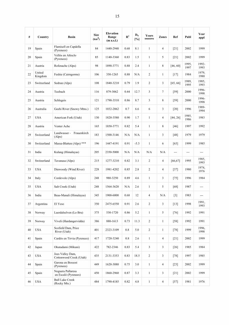
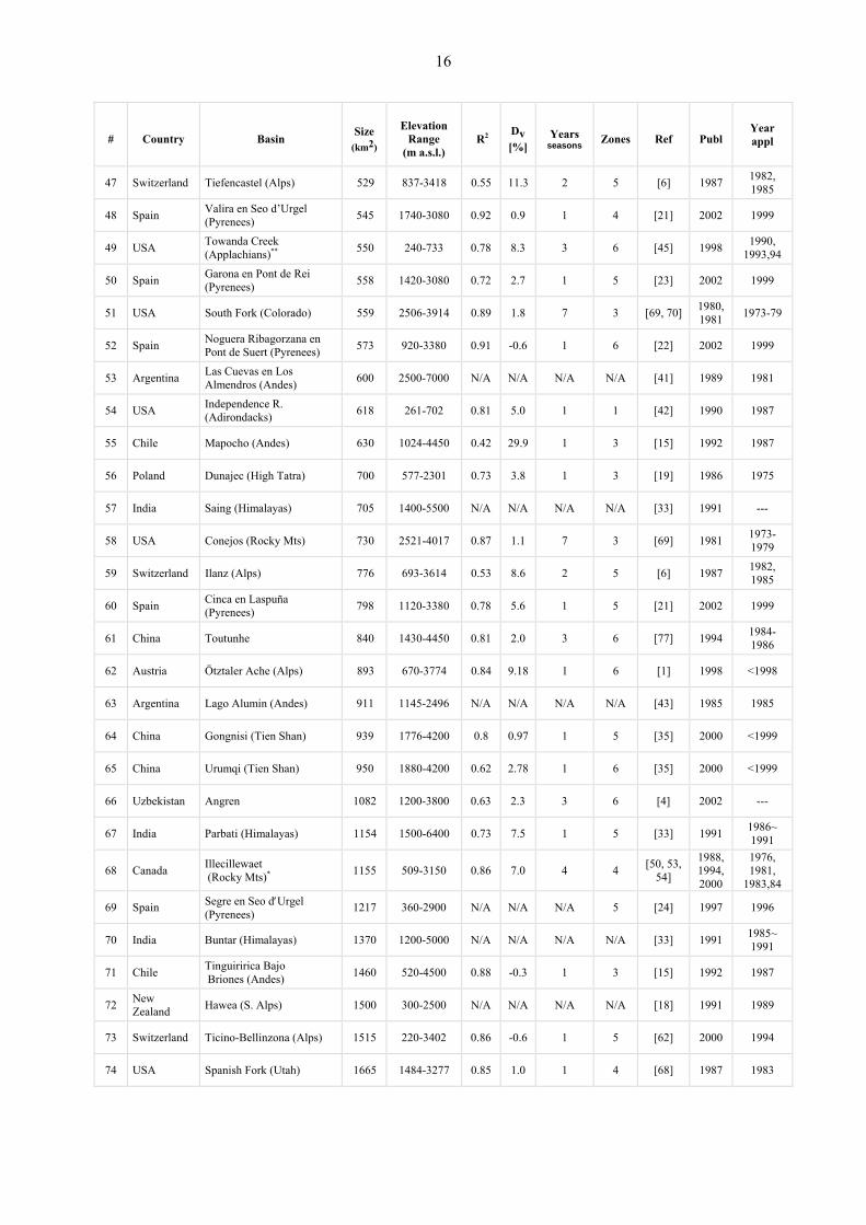
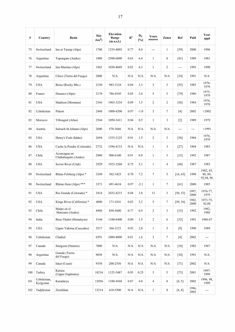
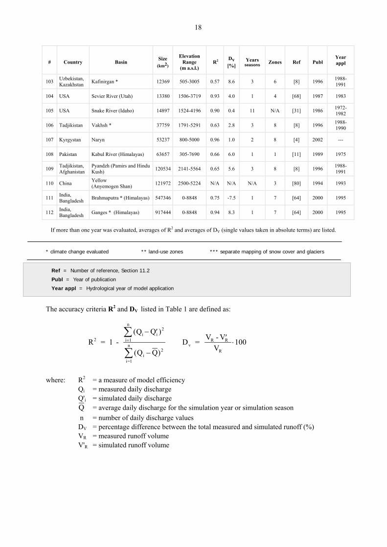
List of Tables Table 1. SRM applications and results. ........................................................................................... 14

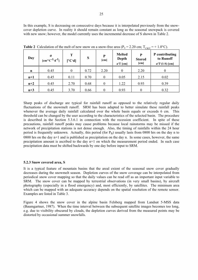
Table 2. Calculation of the melt of new snow deposited on a snow-free area (Pn = 2.20 cm; TCRIT = +

1.0°C). ............................................................................................................................... 25

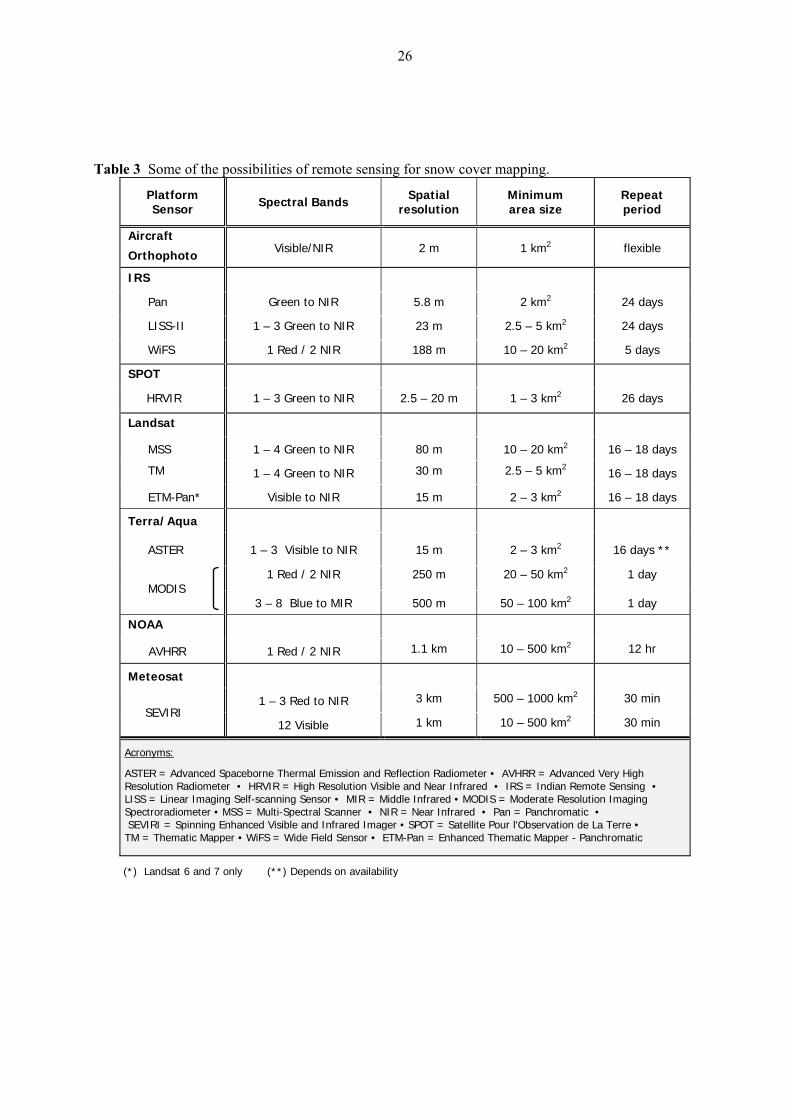
Table 3. Some of the possibilities of remote sensing for snow cover mapping. ................................... 26

Table 4. Results of model performances in the WMO project (10 years, snowmelt season). ................ 46

Table 5. Errors experienced by SRM users and their correction. ........................................................ 49

Table 6. Seasonal redistribution of runoff for 1979 in the Rio Grande near Del Norte, Colorado due to

climate change. .................................................................................................................. 69

Table 7. Seasonal redistribution of runoff for a normalized year in the Rio Grande near Del Norte,

Colorado due to climate change. .......................................................................................... 72

Table 8. Elevation zones and glacier areas in the Illecillewaet basin. ................................................. 78

Table 9. WinSRM capabilities and limitations. .................................................................................. 85

1213

SNOWMELT RUNOFF MODEL (SRM) USER'S MANUAL

(UPDATED EDITION 2008, WINDOWS VERSION 1.11)

1 PREFACE

This 2008 edition of the User’s Manual presents a new computer program, the Windows Version 1.11 of the Snowmelt Runoff Model (WinSRM). The popular Version 4 is also preserved in the Appendix because it is still in demand to be used within its limits. The Windows version adds new capabilities: it accepts more detailed climate scenarios; for example, different daily changes of temperature and precipitation. It makes possible to substitute a data set of temperatures and precipitation of a selected year as a “climate scenario” for any available existing year and evaluate the resulting snow conditions and runoff. A normalized year, including normalized Conventional Depletion Curves (CDC’s) from long term temperature and precipitation data can be derived to represent today’s climate. It is now possible to divide a basin into as many as 16 elevation or other zones in order to refine the modeling, while Version 4 only allowed 8. These improvements facilitate new developments in SRM applications which are already taking place: runoff modeling by using different land use zones, separating satellite mapping of snow and glaciers, runoff modeling in very large basins with an extreme elevation range, and others. The specific features of WinSRM Version 1.11 are explained in detail in this document in Sections 8.5, 8.6, 9, and 10. WinSRM Version 1.11 has been developed without sacrificing the advantages of the SRM Version 4, in particular the speed of getting results. Both versions are available on the Internet by accessing http://www.ars.usda.gov/Services/docs.htm?docid=8872. Should this link not be “current” for the reader, one can “search” on “SRM home” or “WinSRM” to locate a “current site”. So far, four SRM workshops (in 1992, 1994, 1996, and 1998) have been organized at the University of Bern, Switzerland, with about 130 participants from 20 countries taking part. A fifth SRM workshop was organized in 2005 at New Mexico State University. In addition, the authors are available to assist users in overcoming special problems which may be encountered.

2 INTRODUCTION

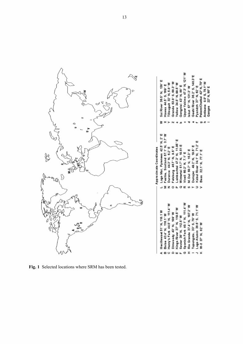
The Snowmelt-Runoff Model (SRM) is designed to simulate and forecast daily streamflow in mountain basins where snowmelt is a major runoff factor. Most recently, it has also been applied to evaluate the effect of a changed climate on seasonal snow cover and runoff. SRM was developed by Martinec (1975) in small European basins. Thanks to the progress of satellite remote sensing of snow cover, SRM has been applied to larger and larger basins. Recently, the runoff was modelled in the basin of the Ganges River, which has an area of 917,444 km2 and an elevation range from 0 to 8,840 m a.s.l. Contrary to the original assumptions, there appear to be no limits for application with regard to the basin size and the elevation range. Also, a dominant role of snowmelt does not seem to be a necessary condition. It is, however, advisable to carefully evaluate the formula for the recession coefficient. Runoff computations by SRM appear to be relatively easily understood. To date the model has been applied by various agencies, institutes and universities in over 100 basins, situated in 29 different countries as listed in Table 1. More than 80% of these applications have been performed by independent users, as is evident from 80 references to pertinent publications. Some of the localities are shown in Figure 1. SRM also successfully underwent tests by the World Meteorological Organization with regard to runoff simulations (WMO, 1986) and to partially simulated conditions of real time runoff forecasts (WMO, 1992).

http://www.ars.usda.gov/Services/docs.htm?docid=8872

13

Fig. 1 Selected locations where SRM has been tested.

14

3 RANGE OF CONDITIONS FOR MODEL APPLICATION

SRM can be applied in mountain basins of almost any size (so far from 0.76 to 917,444 km2) and any elevation range (Table 1). A model run starts with a known or estimated discharge value and can proceed for an unlimited number of days, as long as the input variables - temperature, precipitation and snow covered area - are provided. As a test, a 10-year period was computed without reference to measured discharges (Martinec & Rango, 1986). The references pertinent to the following table can be seen in Section 11.2 “Specific references for Table 1” at the end of this manual. These references appear under the heading "Ref" and with a number to easily find them in Section 11.2. Table 1 SRM applications and results

# Country Basin Size

(km2)

Elevation Range

(m a.s.l.) R2 Dv

[%] Years

seasons Zones Ref Publ Year appl

1 USA EGL (Rocky Mountains) 0.29 3300-3450 N/A N/A N/A N/A [72] 1991 1989

2 USA WGL (Rocky Mountains) 0.6 3300-3450 N/A N/A N/A N/A [72] 1991 1989

3 Germany Lange Bramke (Harz) 0.76 540-700 N/A N/A 1 1 [25] 1984 1981

4 Germany Wintertal (Harz) 0.76 560-754 N/A N/A 1 1 [25] 1984 1981

5 Czech R. Modry Dul (Krkonose) 2.65 1000-1554 0.96 1.7 2 1 [40, 12] 1963, 1970

1962, 1966

6 USA GLEES (Rocky M.) 2.87 3300-3450 N/A N/A N/A N/A [72] 1991 1989

7 Ecuador Antisana (Andes) 3.72 4500-5760 N/A N/A 1 3 [19] 1997 1996

8 Argentina Echaurren 4.5 3000-4200 0.84 7.5 1 1 [14] 1997 1985

9 Spain Lago Mar (Pyrenees) 4.5 2234-3004 N/A N/A 1 1 [39] 1966 1965

10 Spain Llauset dam (Pyrenees) 7.8 2100-3000 0.69 5.5 1 2 [23] 2001 1999

11 USA W-3 (Appalachians) 8.42 346-695 0.81 8.8 10 1 [79] 1986 1969-1978

12 Germany Lainbachtal (Allgauer Alps) 18.7 670-1800 N/A N/A 5 1 [74] 1978 1978,

1979

13 Spain Salenca en Baserca (Pyrenees) 22.2 1460-3200 0.72 4.3 3 3 [22] 2002 1999

14 Spain Noguera Ribagorzana en Baserca (Pyrenees) 36.8 1480-3000 0.71 3.7 3 2 [22] 2002 1995

15 Switzerland Rhone-Gletsch (Alps) 38.9 1755-3630 N/A N/A 1 4 [49] 1980 1979

16 Switzerland Dischma (Alps) 43.3 1668-3146 0.86 2.5 10 3 [38, 79] 1975, 1986

1973, 1970-79

17 Japan Sai (Japan Alps) 57 300-1600 0.86 N/A 3 3 [28, 29, 30]

1982, 1987

1979-1981

18 Spain Tor en Alins (Pyrenees) 60 1880-3040 0.71 7.3 1 4 [21] 2002 1999

15


(km2)

Elevation Range

(m a.s.l.) R2 Dv

[%] Years


19 Spain Flamisell en Capdella (Pyrenees) 84 1440-2940 0.68 8.1 1 4 [21] 2002 1999

20 Spain Vellós en Añisclo (Pyrenees) 85 1140-3360 0.83 1.5 1 5 [21] 2002 1999

21 Austria Rofenache (Alps) 98 1890-3771 0.88 2.4 1 8 [46, 60] 1995, 1997

1992-1993

22 United Kingdom Feshie (Cairngorms) 106 350-1265 0.88 N/A 2 1 [17] 1984 1979,

1980

23 Switzerland Sedrun (Alps) 108 1840-3210 0.79 1.9 2 3 [65, 66] 1989, 1995

1985, 1993

24 Austria Tuxbach 116 879-3062 0.44 12.7 3 7 [59] 2000 1996-1998

25 Austria Schlegeis 121 1790-3510 0.86 8.7 3 8 [59] 2000 1996-1998

26 Australia Geehi River (Snowy Mtns.) 125 1032-2062 0.7 6.6 6 3 [20] 1996 1989-1994

27 USA American Fork (Utah) 130 1820-3580 0.90 1.7 1 4 [44, 26] 1985, 1986 1983

28 Austria Venter Ache 165 1850-3771 0.82 5.4 1 8 [46] 1997 1992

29 Switzerland Landwasser - Frauenkirch (Alps) 183 1500-3146 N/A N/A 1 3 [48] 1979 1979

30 Switzerland Massa-Blatten (Alps) *** 196 1447-4191 0.91 -5.3 1 6 [63] 1999 1985

31 India Kulang (Himalayas) 205 2350-5000 N/A N/A N/A N/A --- --- ---

32 Switzerland Tavanasa (Alps) 215 1277-3210 0.82 3.1 2 4 [66,67] 1995 1985, 1993

33 USA Dinwoody (Wind River) 228 1981-4202 0.85 2.8 2 4 [37] 1980 1974, 1976

34 Italy Cordevole (Alps) 248 980-3250 0.89 4.6 1 3 [75] 1996 1984

35 USA Salt Creek (Utah) 248 1564-3620 N/A 2.6 1 5 [68] 1987 ---

36 India Beas-Manali (Himalayas) 345 1900-6000 0.68 12 4 N/A [3] 1983 ---

37 Argentina El Yeso 350 2475-6550 0.91 2.6 2 3 [13] 1998 1991, 1993

38 Norway Laerdalselven (Lo Bru) 375 530-1720 0.86 5.2 1 5 [76] 1992 1991

39 Norway Viveli (Hardangervidda) 386 880-1613 0.73 11.3 2 1 [58] 1992 1991

40 USA Scofield Dam, Price River (Utah) 401 2323-3109 0.8 5.0 2 1 [78] 1999 1996,

1998

41 Spain Cardós en Tirvia (Pyrenees) 417 1720-3240 0.8 2.6 1 4 [21] 2002 1999

42 Japan Okutadami (Mikuni) 422 782-2346 0.83 5.4 3 3 [26] 1985 1984

43 USA Joes Valley Dam, Cottonwood Creek (Utah) 435 2131-3353 0.83 18.5 2 3 [78] 1997 1985

44 Spain Garona en Bossost (Pyrenees) 449 1620-3080 0.75 3.0 1 4 [23] 2002 1999

45 Spain Noguera Pallaresa en Escaló (Pyrenees) 450 1860-2960 0.87 3.3 1 3 [21] 2002 1999

46 USA Bull Lake Creek (Rocky Mts.) 484 1790-4185 0.82 4.8 1 4 [57] 1981 1976

16


(km2)

Elevation Range

(m a.s.l.) R2 Dv

[%] Years


47 Switzerland Tiefencastel (Alps) 529 837-3418 0.55 11.3 2 5 [6] 1987 1982, 1985

48 Spain Valira en Seo d’Urgel (Pyrenees) 545 1740-3080 0.92 0.9 1 4 [21] 2002 1999

49 USA Towanda Creek (Applachians)** 550 240-733 0.78 8.3 3 6 [45] 1998 1990,

1993,94

50 Spain Garona en Pont de Rei (Pyrenees) 558 1420-3080 0.72 2.7 1 5 [23] 2002 1999

51 USA South Fork (Colorado) 559 2506-3914 0.89 1.8 7 3 [69, 70] 1980, 1981 1973-79

52 Spain Noguera Ribagorzana en Pont de Suert (Pyrenees) 573 920-3380 0.91 -0.6 1 6 [22] 2002 1999

53 Argentina Las Cuevas en Los Almendros (Andes) 600 2500-7000 N/A N/A N/A N/A [41] 1989 1981

54 USA Independence R. (Adirondacks) 618 261-702 0.81 5.0 1 1 [42] 1990 1987

55 Chile Mapocho (Andes) 630 1024-4450 0.42 29.9 1 3 [15] 1992 1987

56 Poland Dunajec (High Tatra) 700 577-2301 0.73 3.8 1 3 [19] 1986 1975

57 India Saing (Himalayas) 705 1400-5500 N/A N/A N/A N/A [33] 1991 ---

58 USA Conejos (Rocky Mts) 730 2521-4017 0.87 1.1 7 3 [69] 1981 1973-1979

59 Switzerland Ilanz (Alps) 776 693-3614 0.53 8.6 2 5 [6] 1987 1982, 1985

60 Spain Cinca en Laspuña (Pyrenees) 798 1120-3380 0.78 5.6 1 5 [21] 2002 1999

61 China Toutunhe 840 1430-4450 0.81 2.0 3 6 [77] 1994 1984- 1986

62 Austria Ötztaler Ache (Alps) 893 670-3774 0.84 9.18 1 6 [1] 1998 <1998

63 Argentina Lago Alumin (Andes) 911 1145-2496 N/A N/A N/A N/A [43] 1985 1985

64 China Gongnisi (Tien Shan) 939 1776-4200 0.8 0.97 1 5 [35] 2000 <1999

65 China Urumqi (Tien Shan) 950 1880-4200 0.62 2.78 1 6 [35] 2000 <1999

66 Uzbekistan Angren 1082 1200-3800 0.63 2.3 3 6 [4] 2002 ---

67 India Parbati (Himalayas) 1154 1500-6400 0.73 7.5 1 5 [33] 1991 1986~ 1991

68 Canada Illecillewaet (Rocky Mts)* 1155 509-3150 0.86 7.0 4 4 [50, 53,

54]

1988, 1994, 2000

1976, 1981,

1983,84

69 Spain Segre en Seo d′Urgel (Pyrenees) 1217 360-2900 N/A N/A N/A 5 [24] 1997 1996

70 India Buntar (Himalayas) 1370 1200-5000 N/A N/A N/A N/A [33] 1991 1985~ 1991

71 Chile Tinguiririca Bajo Briones (Andes) 1460 520-4500 0.88 -0.3 1 3 [15] 1992 1987

72 New Zealand Hawea (S. Alps) 1500 300-2500 N/A N/A N/A N/A [18] 1991 1989

73 Switzerland Ticino-Bellinzona (Alps) 1515 220-3402 0.86 -0.6 1 5 [62] 2000 1994

74 USA Spanish Fork (Utah) 1665 1484-3277 0.85 1.0 1 4 [68] 1987 1983

17


(km2)

Elevation Range

(m a.s.l.) R2 Dv

[%] Years


75 Switzerland Inn at Tarasp (Alps) 1700 1235-4005 0.77 8.0 --- 1 [59] 2000 1996

76 Argentina Tupungato (Andes) 1800 2500-6000 0.63 6.4 1 8 [41] 1989 1981

77 Switzerland Inn-Martina (Alps) 1943 1030-4049 0.82 4.3 1 2 --- 1995 1990

78 Argentina Chico (Tierra del Fuego) 2000 N/A N/A N/A N/A N/A [34] 1991 N/A

79 USA Boise (Rocky Mts.) 2150 983-3124 0.84 3.3 3 3 [55] 1985 1976- 1978

80 France Durance (Alps) 2170 786-4105 0.85 2.6 5 5 [79] 1986 1975- 1979

81 USA Madison (Montana) 2344 1965-3234 0.89 1.5 2 2 [56] 1984 1976, 1978

82 Uzbekistan Pskem 2448 1000-4200 0.97 -1.0 3 7 [4] 2002 <2002

83 Morocco Tillouguit (Atlas) 2544 1050-3411 0.84 0.5 1 3 [2] 1989 1979

84 Austria Salzach-St.Johann (Alps) 2600 570-3666 N/A N/A N/A N/A --- --- >1991

85 USA Henry's Fork (Idaho) 2694 1553-3125 0.91 1.5 2 3 [56] 1984 1976, 1979

86 USA Cache la Poudre (Colorado) 2732 1596-4133 N/A N/A 1 3 [27] 1984 1983

87 Chile Aconcagua en Chababuquito (Andes) 2900 900-6100 0.91 0.9 1 3 [15] 1992 1987

88 USA Sevier River (Utah) 2929 1923-3260 0.75 5.1 1 4 [68] 1987 1983

89 Switzerland Rhine-Felsberg (Alps) * 3249 562-3425 0.70 7.2 7 5 [16, 65] 1998 1982, 85,

88, 89, 92,94, 96

90 Switzerland Rhône-Sion (Alps) *** 3371 491-4634 0.97 -2.1 1 7 [61] 2000 1985

91 USA Rio Grande (Colorado) * 3414 2432-4215 0.84 3.8 13 3 [50, 52] 1997, 2000

1976-77, 1979

92 USA Kings River (California) * 4000 171-4341 0.82 3.2 5 7 [50, 36] 1982, 2000

1973-75, 82,88

93 Chile Maipo en el Manzano (Andes) 4960 850-5600 0.77 0.9 2 3 [15] 1992 1982,

1988

94 India Beas-Thalot (Himalayas) 5144 1100-6400 0.80 1.5 2 6 [32] 1991 1986-87

95 USA Upper Yakima (Cascades) 5517 366-2121 0.92 2.8 1 5 [9] 1990 1989

96 Uzbekistan Chatkal 6591 1000-4000 0.81 1.6 3 7 [4] 2002 ---

97 Canada Sturgeon (Ontario) 7000 N/A N/A N/A N/A N/A [10] 1982 1967

98 Argentina Grande (Tierra del Fuego) 9050 N/A N/A N/A N/A N/A [34] 1991 N/A

99 Canada Iskut (Coast) 9350 200-2556 N/A N/A N/A N/A [71] 2002 N/A

100 Turkey Karasu (Upper Euphrates) 10216 1125-3487 0.95 0.25 3 5 [73] 2001 1997-

1999

101 Uzbekistan, Kyrgystan Karadarya 12056 1100-4568 0.87 4.0 4 8 [4, 5] 2002 1996, 98,

1999

102 Tadjikistan Zerafshan 12214 410-5500 N/A N/A 1 8 [4, 8] 1996, 2002 ---

18


(km2)

Elevation Range

(m a.s.l.) R2 Dv

[%] Years


103 Uzbekistan, Kazakhstan Kafinirgan * 12369 505-3005 0.57 8.6 3 6 [8] 1996 1988-

1991

104 USA Sevier River (Utah) 13380 1506-3719 0.93 4.0 1 4 [68] 1987 1983

105 USA Snake River (Idaho) 14897 1524-4196 0.90 0.4 11 N/A [31] 1986 1972-1982

106 Tadjikistan Vakhsh * 37759 1791-5291 0.63 2.8 3 8 [8] 1996 1988-1990

107 Kyrgystan Naryn 53237 800-5000 0.96 1.0 2 8 [4] 2002 ---

108 Pakistan Kabul River (Himalayas) 63657 305-7690 0.66 6.0 1 1 [11] 1989 1975

109 Tadjikistan, Afghanistan

Pyandzh (Pamirs and Hindu Kush) 120534 2141-5564 0.65 5.6 3 8 [8] 1996 1988-

1991

110 China Yellow (Anyemogen Shan) 121972 2500-5224 N/A N/A N/A 3 [80] 1994 1993

111 India, Bangladesh Brahmaputra * (Himalayas) 547346 0-8848 0.75 -7.5 1 7 [64] 2000 1995

112 India, Bangladesh Ganges * (Himalayas) 917444 0-8848 0.94 8.3 1 7 [64] 2000 1995

If more than one year was evaluated, averages of R2 and averages of DV (single values taken in absolute terms) are listed.

* climate change evaluated ** land-use zones *** separate mapping of snow cover and glaciers

Ref = Number of reference, Section 11.2

Publ = Year of publication

Year appl = Hydrological year of model application
The accuracy criteria R2 and DV listed in Table 1 are defined as:
R = 1 - Q Q )

(Q Q) D = V - V

V1002

i ii 1

n2

i2

i=1

n vR R

R

( − ′

−

′⋅=

∑

∑

where: R2 = a measure of model efficiency Qi = measured daily discharge Q'i = simulated daily discharge Q = average daily discharge for the simulation year or simulation season n = number of daily discharge values DV = percentage difference between the total measured and simulated runoff (%) VR = measured runoff volume V'R = simulated runoff volume

19

In addition to the input variables, the area-elevation curve of the basin is required. If other basin characteristics are available (forested area, soil conditions, antecedent precipitation, and runoff data), they are of course useful for facilitating the determination of the model parameters. SRM can be used for the following purposes:

(1) Simulation of daily flows in a snowmelt season, in a year, or in a sequence of years. The results can be compared with the measured runoff in order to assess the performance of the model and to verify the values of the model parameters. Simulations can also serve to evaluate runoff patterns in ungauged basins using satellite monitoring of snow covered areas and extrapolation of temperatures and precipitation from nearby stations.

(2) Short term and seasonal runoff forecasts. The computer program (WinSRM) includes a derivation of modified depletion curves which relate the snow covered areas to the cumulative snowmelt depths as computed by SRM. These curves enable the snow coverage to be extrapolated manually by the user several days ahead by temperature forecasts so that this input variable is available for discharge forecasts. The modified depletion curves can also be used to evaluate the snow reserves for seasonal runoff forecasts. The model performance may deteriorate if the forecasted air temperature and precipitation deviate from the observed values, but the inaccuracies can be reduced by periodic updating.

(3) In recent years, SRM was applied to the new task of evaluating the potential effect of climate change on the seasonal snow cover and runoff, as explained in Chapter 8. The microcomputer program has been modified and supplemented accordingly.

4 MODEL STRUCTURE

Each day, the water produced from snowmelt and from rainfall is computed, superimposed on the calculated recession flow and transformed into daily discharge from the basin according to Equation (1):

Qn+1 = [cSn · an (Tn + ∆ Tn) Sn+ cRn Pn] A 10000

86400⋅

(1-kn+1) + Qn kn+1 (1)

where: Q = average daily discharge [m3s-1]

c = runoff coefficient expressing the losses as a ratio (runoff/precipitation), with cS referring to snowmelt and cR to rain

a = degree-day factor [cm oC-1d-1] indicating the snowmelt depth resulting from 1 degree-day

T = number of degree-days [oC d]

∆ T = the adjustment by temperature lapse rate when extrapolating the temperature from the station to the average hypsometric elevation of the basin or zone [oC d]

S = ratio of the snow covered area to the total area

P = precipitation contributing to runoff [cm]. A preselected threshold temperature, TCRIT, determines whether this contribution is rainfall and immediate. If precipitation is determined by TCRIT to be new snow, it is kept on storage over the hitherto snow free area until melting conditions occur.

A = area of the basin or zone [km2]

20

k = recession coefficient indicating the decline of discharge in a period without snowmelt or

rainfall:

k = QQ

m+1

m

(m, m + 1 are the sequence of days during a true recession flow period).

n = sequence of days during the discharge computation period. Equation (1) is written for a time lag between the daily temperature cycle and the resulting discharge cycle of 18 hours. In this case, the number of degree-days measured on the nth day corresponds to the discharge on the n + 1 day. Various lag times can be introduced by a subroutine.

1000086400

= conversion from cm·km2d-1 to m3 s-1

T, S and P are variables to be measured or determined each day, cR, cS, lapse rate to determine ∆ T, TCRIT, k and the lag time are parameters which are characteristic for a given basin or, more generally, for a given climate. A guidance for determining these parameters will be given in Section 5.3. If the elevation range of the basin exceeds 500 m, it is recommended that the basin be subdivided into elevation zones of about 500 m each. For an elevation range of 1500 m and three elevation zones A, B and C, the model equation becomes:

( )[ ]

( )[ ]

( )[ ] ( ) 11

1

186400

100086400

100086400

1000

++

+

+−⎭⎬⎫⋅

+∆+

+⋅

+∆+

+⎩⎨⎧ ⋅

+∆+=

nnnC

CnRCnCnCnnCnSCn

BBnRBnBnBnnBnSBn

AAnRAnAnAnnAnSAnn

kQkA

PcSTTac

APcSTTac

APcSTTacQ

(2)

The indices A, B and C refer to the respective elevation zones and a time lag of 18 hours is assumed. Other time lags can be selected and automatically taken into account as explained in the Section 5.3.7. In the simulation mode, SRM can function without updating. The discharge data serve only to evaluate the accuracy of simulation. In ungauged basins the simulation is started with a discharge estimated by analogy to a nearby gauged basin. In the forecasting mode, the model provides an option for updating by the actual discharge every 1-9 days. Equations (1) and (2) are written for the metric system but an option for model operation in English units is also provided in the computer program.

21

5 NECESSARY DATA FOR RUNNING THE MODEL

5.1 Basin characteristics

5.1.1 Basin and zone areas

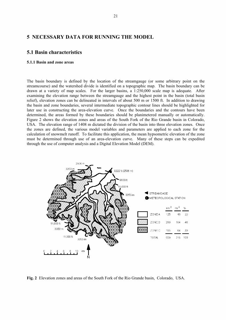
The basin boundary is defined by the location of the streamgauge (or some arbitrary point on the streamcourse) and the watershed divide is identified on a topographic map. The basin boundary can be drawn at a variety of map scales. For the larger basins, a 1:250,000 scale map is adequate. After examining the elevation range between the streamgauge and the highest point in the basin (total basin relief), elevation zones can be delineated in intervals of about 500 m or 1500 ft. In addition to drawing the basin and zone boundaries, several intermediate topographic contour lines should be highlighted for later use in constructing the area-elevation curve. Once the boundaries and the contours have been determined, the areas formed by these boundaries should be planimetered manually or automatically. Figure 2 shows the elevation zones and areas of the South Fork of the Rio Grande basin in Colorado, USA. The elevation range of 1408 m dictated the division of the basin into three elevation zones. Once the zones are defined, the various model variables and parameters are applied to each zone for the calculation of snowmelt runoff. To facilitate this application, the mean hypsometric elevation of the zone must be determined through use of an area-elevation curve. Many of these steps can be expedited through the use of computer analysis and a Digital Elevation Model (DEM).

Fig. 2 Elevation zones and areas of the South Fork of the Rio Grande basin, Colorado, USA.

22

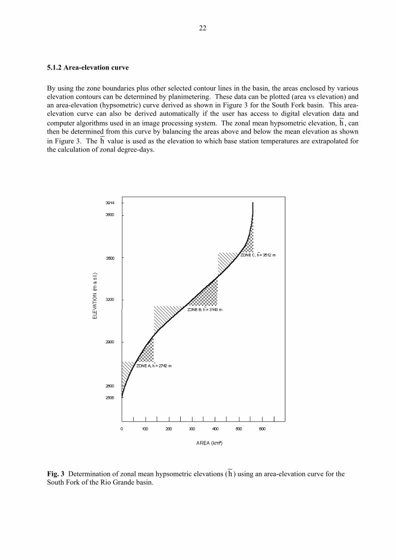
5.1.2 Area-elevation curve

By lines in the basin, the areas enclosed by various elevation contours can be determined by planimetering. These data can be plotted (area vs elevation) and a ar urve derived as shown in Figure 3 for the South Fork basin. This area-elevation curve can also be derived automatically if the user has access to digital elevation data and computer algorithms used in an image processing system. The zonal mean hypsometric elevation,

using the zone boundaries plus other selected contour

n ea-elevation (hypsometric) c

h , can lancing the areas above and below the mean elevation as shown then be determined from this curve by ba

in Figure 3. The h value is used as the elevation to which base station temperatures are extrapolated for the calculation of zonal degree-days.

Fig. 3 Determination of zonal mean hypsometric elevations (h ) using an area-elevation curve for the South Fork of the Rio Grande basin.

23

5.2 Variables

- TEMPERATURE

- PRECIPITATION

- SNOW COVERED AREA

5.2.1 Temperature and degree-days, T In order to compute the daily snowmelt depths, the number of degree-days must be determined from temperature measurements or, in a forecasting mode, from temperature forecasts. Temperature average Program options: 0 = daily mean 1 = Min, Max The program accepts either the daily mean temperature (option 0) or two temperature values on each day: TMax, TMin (option 1). The temperatures are extrapolated by the program from the base station elevation to the hypsometric mean elevations of the respective elevation zones. For option 1, the average temperature

computed in each zone as is

T = T + TMax Min 2

(3)

When using daily means (option 0) or when using TMax, TMin (option 1), it is recommended that negative temperature values (when they occur) be used in the calculation. In line with this recommendation, the original "effective minimum temperature" alternative (automatic change of negative temperatures to 0°C) was removed from the computer program beginning with Version 3.0. If the user still prefers this alternative, the occasional negative temperatures can be changed manually to 0°C when inputting the data to SRM. Because the average temperatures refer to a 24 hour period starting always at 0600 hrs, they become degree-days T [°C·d]. The altitude adjustment ∆T in Equation (1) is computed as follows:

∆T = (h - h) . 1100stγ ⋅ (4)

where γ = temperature lapse rate [°C per 100 m] hst = altitude of the temperature station [m]

h = hypsometric mean elevation of a zone [m] Whenever the degree-day numbers (T + ∆ T in Equation (1)) become negative, they are automatically set to zero so that no negative snowmelt is computed. The values of the temperature lapse rate are dealt with in Section 5.3.3.

Temperature input Program options: 0 = basin wide 1 = by zone

24

The program accepts either temperature data from a single station (option 0, basin wide) or from several stations (option 1, by zone). With option 0, the altitude of the station is entered and temperature data are extrapolated to the hypsometric mean elevations of all zones using the lapse rate. If more stations are vailable, the user can prepare a single "synthetic station" and still use option 0 or, alternatively, use ption 1. With option 1, the user may use separate stations for each elevation zone, however, the

ion of the zone. Although SRM will take separate stations for each zone in this way, it is optional. The measurement of correct air tem atures is ifficult, there good t perature station (even if located outside the basin) ma ferabl sever relia ns.

In the forecast mode of the model, it is necessary to obtain representative temperature forecasts for the give egion an de in ord to extr e the ted num rs of de ays for eac levation zon 5.2.2 Precipitation, P

h luation resentat eal p tation particul ifficult i ountain basins. Also, uantitative precipitation forecasts are seldom available for the forecast mode, although current efforts in

all other zones. Otherwise o precipitation from these zones is taken into account by the program. Further program options refer to e rainfall contributing area as explained in Section 5.3.5. In basins with a great elevation range, the

derestimated if only low altitude precipitation stations are available. It is precipitation data to the mean hypsometric altitudes of the respective zones

on 5.3.4) is used to decide whether a precipitation event will be treated as in (T ≥ T ) or as new snow ( T < T ). When the precipitation event is determined to be snow, its

g over the snow-free area is considered as precipitation to be added to snowmelt, with this effect delayed until the next day warm enough to produce melting. This precipitation is stored by SRM and then melted as soon as a sufficient number of degree-days has occurred. The following example in Table 2 illustrates a case where 2.20 cm water equivalent of snow fell on day n and then was melted on the three successive days. This procedure is slightly changed in the winter as it will be explained later.

aotemperatures entered for each zone must have already been lapsed to the mean hypsometric elevat

onlyper d

e toand fore one em

y be pre al less ble statio

n r d altitu er apolat expec be gree-d h ee.

T e eva of rep ive ar recipi is arly d n mqthis field are improving this situation. Fortunately, snowmelt generally prevails over the rainfall component in the mountain basins. However, sharp runoff peaks from occasional heavy rainfalls must be given particular attention and the program includes a special treatment of such events (see Section 5.3.6). Rainfall input Program options: 0 = basin wide 1 = by zone The program accepts either a single, basin-wide precipitation input (from one station or from a "synthetic station" combined from several stations, that is, option 0) or different precipitation inputs zone by zone (option 1). If the program is switched to option 1 and only one station happens to be available, for xample in the zone A, precipitation data entered for zone A must be copied to e

nthprecipitation input may be unrecommended to extrapolate by an altitude gradient, for example 3 % or 4 % per 100 m. If two stations at different altitudes are available, it is possible to assign the averaged data to the average elevation of both stations and to extrapolate by an altitude gradient from this reference level to the elevation zones. It should be noted that the increase of precipitation amounts with altitude does not continue indefinitely but stops at a certain altitude, especially in very high elevation mountain ranges. A critical temperature (see Sectira CRIT CRITdelayed effect on runoff is treated differently depending on whether it falls over the snow-covered or snow-free portion of the basin. The new snow that falls over the previously snow-covered area is assumed to become part of the seasonal snowpack and its effect is included in the normal depletion curve of the snow coverage. The new snow fallin

25

In this example, S is decreasing on consecutive days because it is interpolated previously from the snow-over depletion curve. In reality it should remain constant as long as the seasonal snowpack is covered ith new snow; however, the model currently uses the incremental decrease of S shown in Table 2.

Table 2 n of the melt of new snow on a snow-free area (Pn TCRIT =

D a .°C-1.d-1]

T [

S P [c

MeltedDepth a.T [cm]

P contributing to Runoff

[cm]

cw

Calculatio = 2.20 cm;

P

+ 1.0°C).

ay [cm °C.d] m] Stored

[cm] a.T.(1-S)

n 0.45 0 0.72 2.20 0 2.20 0

n+1 0.45 0.11 .70 0.05 2.15 0 0 0.02

n+2 0.45 2.70 0 1.22 0.68 0.93 0.39

n+3 0.45 3.70 0.93 0.66 0 0 0.32 Sharp peaks of discharge are typical for rainfall runoff as opposed to the relatively regular daily fluct the snowmelt runoff. SRM has been adapted to better simulate these rainfall peaks wheneve average dai ted over hole ba r exc This threshold can be changed by the user according to the characteristics of the selected basin. The procedure is described in the Section 5.3.6.1 in connection with recession precautio l runoff p use problem ause loca ms may if the network of precipitation stations is not dense enough. lso, the timing of rainfalls within the 24 hour period is frequently unknown. Actually, this period (for Pn) usually lasts from 0800 hrs on the day n to 0800 hrs on the day n+1 and is published as precipitati the day n cases, however, the same precipitation amount is ascribed to the day n+1 on wh easurem case precipitation data must be sh s by one d re input

5.2.3 Snow covered area, S

It is eature of mountain basins that the areal extent of the seasonal snow cover gradually decreases during the snowm letion cur the snow coverage can be interpolated from periodic cover mapping so that the daily values SRM. The snow cover can b by terrestri ervation all basins), by aircraft photography (especially in a flood emergency) and, most efficiently, by satellites. The minimum area which can be mapped with an adequate accuracy depends on the spatial resolution of the remote sensor. Exam Figu MSS data (Bau s too long, e.g. nts may be

istorted by occasional summer snowfalls.

uations ofr the ly rainfall calcula the w sin equals o eeds 6 cm.

the coefficient. In spite of these ns, rainfal eaks may ca s bec l rainstor be missed

A

on on . In someich the m

ay befoent period ended.

to SRM. In such

ifted backward

a typical felt season. Dep ves of

can be read off as an imal snow portant input variable to e mapped al obs s (in very sm

ples are listed in Table 3.

re 4 shows the snow cover in the alpine basin Felsberg mapped from Landsat 5-mgartner, 1987). When the time interval between the subsequent satellite images becomedue to visibility obscured by clouds, the depletion curves derived from the measured poi

d

26

Table 3 Some of the possibilities of remote sensing for snow cover mapping.

Platform Sensor Spectral Bands atial

resolution Minimum area size

Repeat period

Sp

Aircraft

Orthophoto Visible/NIR 2 m 1 km2 flexible

IRS

Pan Green to NIR 5.8 m 2 km2 24 days

LISS-II 1 – 3 Green to NIR 23 m 2.5 – 5 km2 24 days

WiFS 1 Red / 2 NIR 188 m 10 – 20 km2 5 days

SPOT

HRVIR 1 – 3 Green to NIR 2.5 – 20 m 1 – 3 km2 26 days

Landsat

MSS 1 – 4 Green to NIR 80 m 10 – 20 km2 16 – 18 days

TM 1 – 4 Green to NIR 30 m 2.5 – 5 km216 – 18 days

ETM-Pan* Visible to NIR 15 m 2 – 3 km2 16 – 18 days

Terra/Aqua

ASTER 1 – 3 Visible to NIR 15 m 2 – 3 km2 16 days **

1 Red / 2 NIR 250 m 20 – 50 km2 1 day MODIS 3 – 8 Blue to MIR 500 m 50 – 100 km2 1 day

NOAA

AVHRR 1 Red / 2 NIR 1.1 km 10 – 500 km2 12 hr

Meteosat

1 – 3 Red to NIR 3 km 500 – 1000 km2 30 min SEVIRI

12 Visible 1 km 10 – 500 km2 30 min

Acronyms: ASTER = Advanced Spaceborne Thermal Emission and Reflection Radiometer • AVHRR = Advanced Very High Resolution Radiometer • HRVIR = High Resolution Visible and Near Infrared • IRS = Indian Remote Sensing • LISS = Linear Imaging Self-scanning Sensor • MIR = Middle Infrared • MODIS = Moderate Resolution Imaging Spectroradiometer • MSS = Multi-Spectral Scanner • NIR = Near Infrared • Pan = Panchromatic • SEVIRI = Spinning Enhanced Visible and Infrared Imager • SPOT = Satellite Pour l'Observation de La Terre • TM = Thematic Mapper • WiFS = Wide Field Sensor • ETM-Pan = Enhanced Thematic Mapper - Panchromatic

(*) Landsat 6 and 7 only (**) Depends on availability

27

Fig. 4 Sequence of snow cover maps from Landsat 5-MSS, Upper Rhine River at Felsberg, 3250 km2 , 560-3614 m a.s.l. (Baumgartner, 1987). Black is snow free area, gray is cloud covered area and white is snow covered area.

28

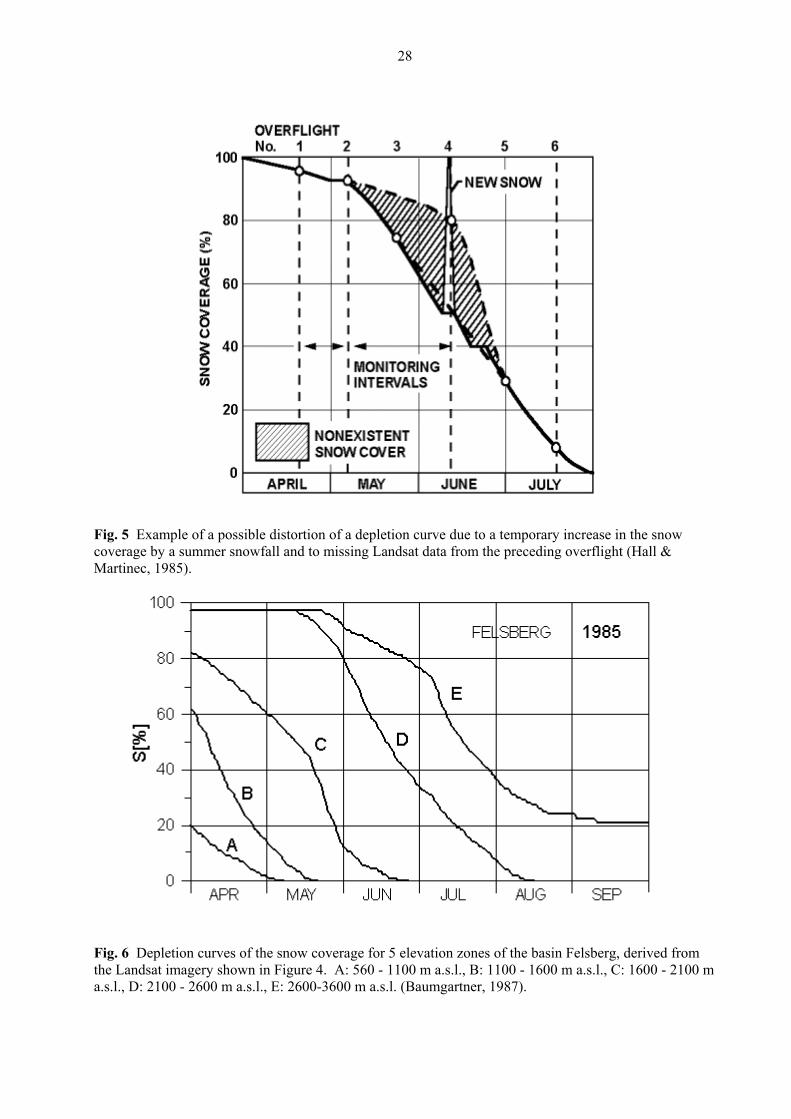
Fig. 5 Example of a possible distortion of a depletion curve due to a temporary increase in the snow coverage by a summer snowfall and to missing Landsat data from the preceding overflight (Hall & Martinec, 1985).

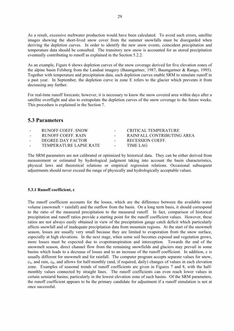
Fig. 6 Depletion curves of the snow coverage for 5 elevation zones of the basin Felsberg, derived from the Landsat imagery shown in Figure 4. A: 560 - 1100 m a.s.l., B: 1100 - 1600 m a.s.l., C: 1600 - 2100 m .s.l., D: 2100 - 2600 m a.s.l., E: 2600-3600 m a.s.l. (Baumgartner, 1987). a

29

As a result, excessive meltwater production would have been calculated. To avoid such errors, satellite images showing the short-lived snow cover from the summer snowfalls must be disregarded when

eriving the dedte

pletion curves. In order to identify the new snow events, coincident precipitation and mperature data should be consulted. The transitory new snow is accounted for as stored precipitation

s an example, Figure 6 shows depletion curves of the snow coverage derived for five elevation zones of

noff forecasts; however, it is necessary to know the snow covered area within days after a tellite overflight and also to extrapolate the depletion curves of the snow coverage to the future weeks.

CRITICAL TEMPERATURE RAINFALL CONTRIBUTING AREA

DEGREE DAY FACTOR - RECESSION COEFF. TEMPERATURE LAPSE RATE

The SRM parame istorical data. They can be either derived from measuremphysical laws anadjustments shoul rologically acceptable values.

5.3.1 Runoff coef

The runoff coefficient accounts for the losses, which are the difference between the available water volume (snowmelto the ratio of thprecipitation and runoff ratios provide a starting point for the runoff coefficient values. However, these

d of inadequate precipitation data from mountain regions. At the start of the snowmelt very small because they are limited to evaporation from the snow surface,

specially at high elevations. ore losses must be expect

snowmelt season, direct channel flow from the remaining snowfields and glaciers may prevail in some hi increase of the runoff coefficient. In addition, c is

dif computer program accepts separate values for snow, S, and rain, cR onthly (and, if required, daily) changes of values in each elevation

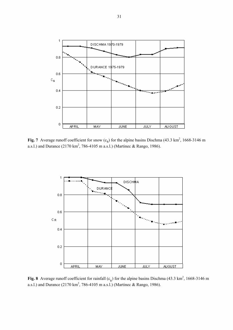
zone. Examples of seasonal trends of runoff coefficients are given in Figures 7 and 8, with the half-onthly values connected by straight lines. The runoff coefficients can even reach lower values in

ertain semiarid basins; particularly in the lowest elevation zone of such basins. Of the SRM parameters, e runoff coefficient appears to be the primary candidate for adjustment if a runoff simulation is not at

eventually contributing to runoff as explained in the Section 5.2.2.

Athe alpine basin Felsberg from the Landsat imagery (Baumgartner, 1987, Baumgartner & Rango, 1995). Together with temperature and precipitation data, such depletion curves enable SRM to simulate runoff in a past year. In September, the depletion curve in zone E refers to the glacier which prevents it from decreasing any further. For real-time rusaThis procedure is explained in the Section 7.

5.3 Parameters

- RUNOFF COEFF. SNOW - - RUNOFF COEFF. RAIN - - - - TIME LAG

ters are not calibrated or optimized by hent or estimated by hydrological judgment taking into account the basin characteristics,

d theoretical relations or empirical regression relations. Occasional subsequent d never exceed the range of physically and hyd

ficient, c

t + rainfall) and the outflow from the basin. On a long term basis, it should correspond e measured precipitation to the measured runoff. In fact, comparison of historical

ratios are not always easily obtained in view of the precipitation gauge catch deficit which particularly affects snowfall anseason, losses are usuallye In the next stage, when some soil becomes exposed and vegetation grows, m ed due to evapotranspiration and interception. Towards the end of the

basins w ch leads to a decrease of losses and to ansually fere for rainfall. Theu nt for snowmelt and

c , and allows for half-m

mcthonce successful.

30

5.3.2 Degree-day factor, a

The degree-day factor a [cm oC-1 d-1] converts the number of degree-days T [oC·d] into the daily snowmelt depth M [cm]:

M = a·T (5)

Degree-day ratios can be evaluated by comparing degree-day values with the daily decrease of the snow water equivalent which is measured by radioactive snow gauge, snow pillow or a snow lysimeter. Such measurements (Martinec, 1960) have shown a considerable variability of degree-day ratios from day to day. This is understandable because the degree-day method does not take specifically into account other components of the energy balance, notably the solar radiation, wind speed and the latent heat of condensation. If averaged for 3-5 days, however, the degree-day factor is more consistent and can represent melting conditions. The effect of daily fluctuations of the degree day values on the runoff from a basin as computed by SRM is greatly reduced because the daily meltwater input is superimposed on the more constant recession flow (Equation (1)). The degree-day method requires several precautions:

ding to the changing snow properties during the snowmelt season.

(2) If point values are applied to areal computations, the degree-day values must be determined for the hypsometric mean elevation of the snow cover in question and not, for example, for the altitude of the snow line.

(3) If the snow cover is scattered, a correctly evaluated degree-day factor will produce less meltwater than if a 100 percent snow cover were assumed. A meltwater difference that arises from erroneous snow cover information should not be compensated for by "optimizing" the degree-day factor. Instead, the correct areal extent of the snow cover should be determined and used.

(4) In large area extrapolations, point measurements should be weighted depending on how well a specific station represents the hydrological characteristics of a given zone (Shafer et al., 1981).

In the absence of detailed data, the degree-day factor can be obtained from an empirical relation (Martinec, 1960):

(1) The degree-day factor is not a constant. It changes accor

a = 1.1 s

w

⋅ρρ

(6)

where a = the degree-day factor [cm °C-1d-1] ρs = density of snow

ρw = density of water

content in snow increases. Thus the snow density is an index of the changing properties which favor the snowmelt.

When the snow density increases, the albedo decreases, and the liquid water

31

Fig. 7 Average runoff coefficient for snow (cs) for the alpine basins Dischma (43.3 km2, 1668-3146 m a.s.l.) and Durance (2170 km2, 786-4105 m a.s.l.) (Martinec & Rango, 1986).

Fig. 8 Average runoff coefficient for rainfall (cR) for the alpine basins Dischma (43.3 km2, 1668-3146 m a.s.l.) and Durance (2170 km2, 786-4105 m a.s.l.) (Martinec & Rango, 1986).

32

Figure 9 illustrates the seasonal trend of the degree-day factor in the Alps and in the Rocky Mountains.Because the geographic latitud

e of a basin influences the solar radiation, it may be advisable to adjust the

egree-day factors accordingly. In glacierized basins, the degree-day factor usually exceeds 0.6 cm C-1d-1 towards the end of the summer when ice becomes exposed (Kotlyakov & Krenke, 1982). The computer

y factors for up to 16 elevation zones which are usually changed twice

tation of snowmelt without changing the structure of SRM. Such refinement appeared to be

d by analogy from other basins or with regard to climatic

d

program accepts different degree-daa month (although daily changes are possible). Sometimes the occurrence of a large, late season snowfall will produce depressed a-values for several days due to the new low-density snow. The a-values in the model can be manually modified and inserted to reflect these unusual snowmelt conditions. As is evident from Equation (1), the degree-day method could be readily replaced by a more refined ompuc

imperative in a study of outflow from a snow lysimeter (Martinec, 1989) but is not considered to be expedient for hydrological basins until the necessary additional variables and their forecasts become available. The degree-day method is explained in more detail in a separate publication (Rango & Martinec, 1995).

5.3.3 Temperature lapse rate, γ

If temperature stations at different altitudes are available, the lapse rate can be predetermined from istorical data. Otherwise it must be evaluateh

conditions. In SRM simulations, a lapse rate of 0.65°C per 100 m was usually employed. Slightly higher, seasonally changing values appeared to be adequate in the Rocky Mountains.

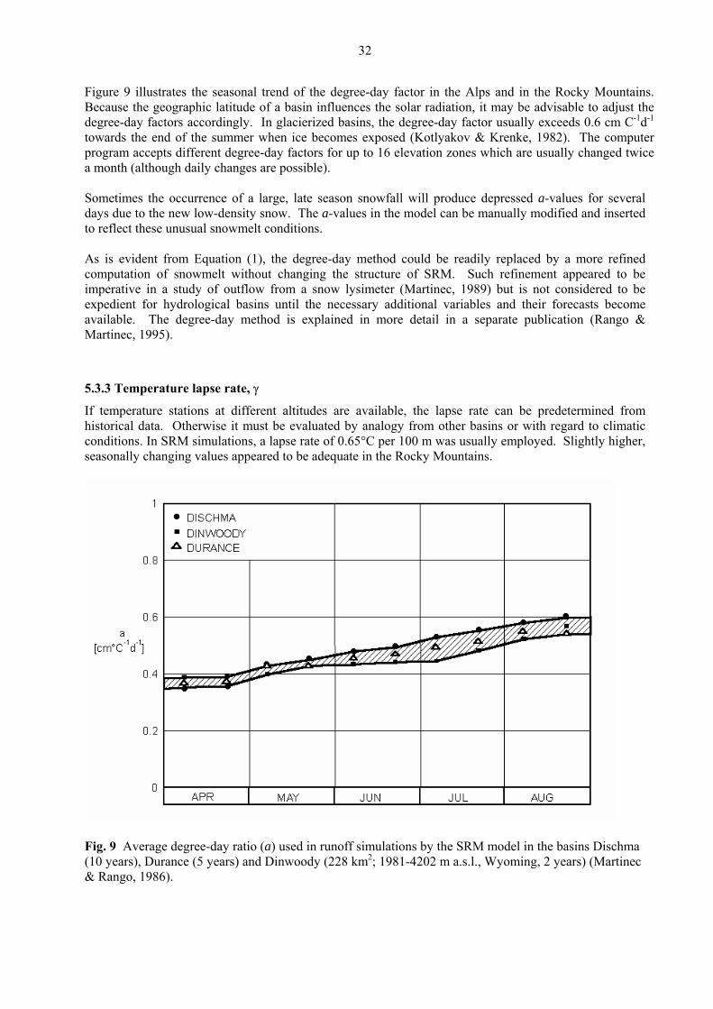
Fig. 9 Average degree-day ratio (a) used in runoff simulations by the SRM model in the basins Dischma

0 years), Durance (5 years) and Dinwoody (228 km2; 1981-4202 m a.s.l., Wyoming, 2 years) (Martinec Rango, 1986).

(1&

33

The computer program accepts either a single or a basin wide lapse rate (option 0) or different rates for ermined lapse

tes every 15 days, and the lapse rate can be changed manually on selected days if a special eteorological situation (for example, a temperature inversion) requires a different value:

emperatur ate Pro ram options:

1 = by zone

the temperature station is situated near the mean elevation of the basin, possible errors in the lapse rate re to some extent canceled out because the extrapolation of temperature takes place upwards as well as

other hand, the temperature station is at a low altitude, SRM becomes sensitive to e lapse rate. For some basins in Wyoming, for example, the closest temperature station was more than

00 km awa e highest snow-covered parts of the basins. In such a case, an rror in the per 100 m causes a deviation of 1 degree-day from the correct egree-day value which corresponds to an error of about 0.5 cm of the computed daily meltwater depth

uch situations sometimes necessitate an adjustment of the originally selected lapse rate taking into ccount the course of the depletion curves of snow coverage. peratures result from

rom a false lapse rate hich must be increased or decreased, depending on whether the temperature station is lower or higher

than the mean zone elevation.

5.3.4 Critical temperature, TCRIT

The critical temperature determines whether the measured or forecasted precipitation is rain or snow. Models which simulate the build-up of the snow cover, first in order to simulate the runoff, depend heavily on this parameter not only in the ablation period; but particularly, in the accumulation period. SRM needs the critical temperature only in order to decide whether precipitation immediately contributes to runoff (rain), or, if T < TCRIT, whether snowfall took place. In this case, SRM automatically keeps the newly fallen snow in storage until it is melted on subsequent warm days, as explained in the Section 5.2.2. When SRM was applied in the alpine basin Dischma, TCRIT started at + 3°C in April at the beginning of snowmelt and diminished to + 0.75°C in July. This seasonal trend with a narrower range appears to be applicable in other basins. At certain times, SRM may not take notice of a sharp rainfall runoff peak because the corresponding precipitation is determined to be snow, the extrapolated temperature being just slightly below the critical temperature. In such cases the assignment of critical temperature and the temperature lapse rate values should be reviewed and logical adjustments made in order to change snow to rain. It is of course difficult to distinguish accurately between rain and snow because the temperature used is the daily mean while precipitation may occur at any time, day or night, i.e., in the warmer or colder portion of the daily temperature cycle. As a possible refinement, formulas have been proposed (Higuchi et al., 1982) to determine the proportion of rain and snow in mixed precipitation conditions.

5.3.5 Rainfall contributing area, RCA

When precipitation is determined to be rain, it can be treated in two ways. In the initial situation (option 0), it is assumed that rain falling on the snowpack early in the snowmelt season is retained by the snow

each zone (option 1). Seasonal variations can also be accommodated by inputting predetram T e lapse r g 0 = basin wide

Ifadownwards. If, on theth1 y and 2000 m lower than the lapse rate of only 0.05°C dlate in the snowmelt season. Sa If high temextrapolation by a certain lapse rate but no change in the snow areal extent is observed, then probably no appreciable snowmelt is taking place at this altitude. The high temperatures result fw

34

which is usually dry and deep. Rainfall runoff is added to snowmelt runoff only from the snow-free area, at is to say the rainfall depth is reduced by the ratio snow-free area/zone area. At some later stage, the

e ter is

from the entire zone area is added to snowmelt. The melting ffect of rain is neglected because the additional heat supplied by the liquid precipitation is considered to e small (Wilson, 1941).

As is evident from Equation (1), the recession coefficient is an important feature of SRM since (1-k) is r production which immediately appears in the runoff. Analysis of

to determine k. Figure 10 shows such an evaluation for the 6 m a.s.l.). Values of Qn and Qn+1 are plotted against each other

nd the lower envelope line of all points is considered to indicate the k-values. Based on the relation k = k1 = 0.677 for Qn = 14 m3s-1 and k2 = 0.85 for Qn = 1 m3s-1.

This means that k is not constant, but increases with the decreasing Q according to the equation:

(7)

or a given basin by solving the equations:

log k1 = log x - y log Q1 (8)

log k2 = log x - y log Q2

the given example,

thsnow cover becomes ripe (the user must decide on which date) and the computer program should bswitched to option 1. Now, if rain falls on this snow cover, it is assumed that the same amount of wareleased from the snowpack so that raineb

5.3.6 Recession coefficient, k

the proportion of the daily meltwatehistorical discharge data is usually a good wayalpine basin Dischma (43.3 km2, 1668-314aQn+1/ Qn, it can be derived that for example

k = x Qn+1 ny⋅ −

where the constants x and y must be determined f k1 = x Q1

y⋅ − k2 = x Q2

y⋅ −

(9)

In log 0.677 = log x - y log 14 log 0.85 = log x - y log 1 x = 0.85 y = 0.086 As a formal change from the SRM User's Manual of 1983 (Martinec et al., 1983), a negative sign appears in the exponent of Equation (7) so that the numerical values of x and y are positive.

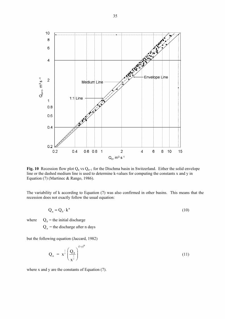
35

Fig. 10

es for computing the constants x and y in quation (7) (Martinec & Rango, 1986).

d in other basins. This means that the cession does not exactly follow the usual equation:

= the discharge after n days

Recession flow plot Qn vs Qn+1 for the Dischma basin in Switzerland. Either the solid envelope line or the dashed medium line is used to determine k-valuE The variability of k according to Equation (7) was also confirmere

Q Q kn 0n= ⋅ (10)

where Q0 = the initial discharge

Qn

but the following equation (Jaccard, 1982)

Q = x Qn

0y1

⎝⎜⎜ ⎠

⎟⎟ 1 ⎛ ⎞

(1-y)n

y

(11) x

where x and y are the constants of Equation (7).

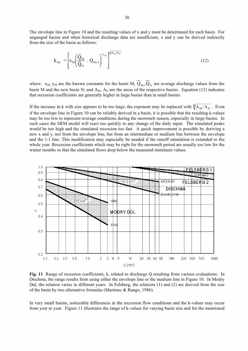
36

The envelope line in Figure 10 and the resulting values of x and y must be determined for each basin. For ungauged basins and when historical discharge data are insufficient, x and y can be derived indirectly from the size of the basin as follows:

!

kNn = xM

QM

QN

. QNn-1

"

# $

%

& '

-yM(

)

* *

+

,

- -

AM /AN4

(12)

where: xM, yM are the known constants for the basin M; Q QM N, are average discharge values from the basin M and the new basin N; and AM, AN are the areas of the respective basins. Equation (12) indicates that recession coefficients are generally higher in large basins than in small basins. If the increase in k with size appears to be too large, the exponent may be replaced with A /A

M N8 . Even

if the envelope line in Figure 10 can be reliably derived in a basin, it is possible that the resulting k-values may be too low to represent average conditions during the snowmelt season, especially in large basins. In such cases the SRM model will react too quickly to any change of the daily input. The simulated peaks would be too high and the simulated recession too fast. A quick improvement is possible by deriving a new x and y, not from the envelope line, but from an intermediate or medium line between the envelope and the 1:1 line. This modification may especially be needed if the runoff simulation is extended to the whole year. Recession coefficients which may be right for the snowmelt period are usually too low for the winter months so that the simulated flows drop below the measured minimum values.

Fig. 11 Range of recession coefficients, k, related to discharge Q resulting from various evaluations: In Dischma, the range results from using either the envelope line or the medium line in Figure 10. In Modry Dul, the relation varies in different years. In Felsberg, the relations (1) and (2) are derived from the size of the basin by two alternative formulas (Martinec & Rango, 1986).

In very small basins, noticeable differences in the recession flow conditions and the k-values may occur from year to year. Figure 11 illustrates the range of k-values for varying basin size and for the mentioned

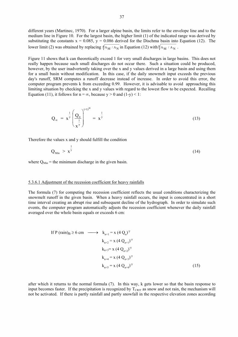
37

different years (Martinec, 1970). For a larger alpine basin, the limits refer to the envelope line and to the edium line in Figure 10. For the largest basin, the higher limit (1) of the indicated range was derived by

substituting the constants x = 0.085, y = 0.086 derived for the Dischma basin into Equation (12). The wer limit (2) was obtained by replacing

m

A M / A N4 in Equation (12) with A M / A N8 . lo

Figure 11 shows that k can theoretically exceed 1 for very small discharges in large basins. This does not really happen because such small discharges do not occur there. Such a situation could be produced,

owever, by the user inadvertently taking over the x and y values derived in a large basin and using them sin without modification. In this case, if the daily snowmelt input exceeds the previous RM computes a runoff decrease instead of increase. In order to avoid this error, the

omputer program prevents k from exceeding 0.99. However, it is advisable to avoid approaching this y values with regard to the lowest flow to be expected. Recalling use y > 0 and (1-y) < 1:

hfor a small baday's runoff, Sclimiting situation by checking the x andEquation (11), it follows for n = ∞, beca

Q = x Q

x= x

1y

y

(<1)1y

∞

∞

⎛

⎝

⎜⎜

⎞

⎠⎟ 0

1⎟⎟

(13)

Therefore the values x and y should fulfill the condition

Q > xMin

1y (14)

here QMin = the minimum discharge in the given basin. w 5.3.6.1 Adjustment of the recession coefficient for heavy rainfalls The formula (7) for computing the recession coefficient reflects the usual conditions characterizing the

heavy rainfall occurs, the input is concentrated in a short quent decline of the hydrograph. In order to simulate such djusts the recession coefficient whenever the daily rainfall ds 6 cm:

If P (rain)n ≥ 6 cm

snowmelt runoff in the given basin. When a time interval creating an abrupt rise and subseevents, the computer program automatically aaveraged over the whole basin equals or excee

⎯ →⎯ kn+1 = x (4 Qn)-y

k 2 = x (4 Qn+1)-y

kn+3= x (4 Qn+2)-y

k = x (4 Q )-y

vation zones according

n+

n+4 n+3

k = x (4 Q )n+5 n+4-y (15)

after which it returns to the normal formula (7). In this way, k gets lower so that the basin response to input becomes faster. If the precipitation is recognized by T as snow and not rain, the mechanism will not be activated. If there is partly rainfall and partly snowfall in the respective ele

CRIT

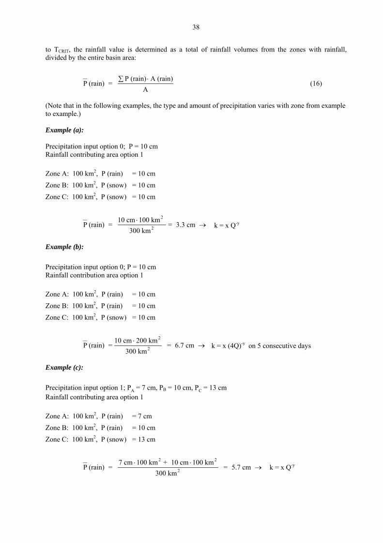
38

to TCRIT, the rainfall value is determined as a total of rainfall volumes from the zones with rainfall, divided by the entire basin area:

P (rain) = A

(16)

(Note that in the following examples, the type and amount of precipitation varies with zone from example to example.) Example (a): Precipitation input option 0; P = 10 cm

ainfall contributing area option 1

P (rain) A (rain)⋅∑

0 km2, P (snow)

R Zone A: 100 km2, P (rain) = 10 cm Zone B: 10 = 10 cmZone C: 100 km2, P (snow) = 10 cm

P (rain) = 10 cm 1 2⋅ 00 km

= 3.3 cm k = x Q-y→ ⋅

k = x Q300 km2

Example (b):

Precipitation input option 0; P = 10 cm Rainfall contribution area option 1

Zone A: 100 km2, P (rain) = 10 cm Zone B: 100 km2, P (rain) = 10 cm

one C: 100 kmZ 2, P (snow) = 10 cm

P (rain) =10 cm 200 km

300 km = 6.7 -y2

2⋅

cm k = x (4Q) on 5 consecutive days→ ⋅

ption 1

= 10 cm

= 13 cm

Example (c):

Precipitation input option 1; PA = 7 cm, PB = 10 cm, PC = 13 cm Rainfall contributing area o Zone A: 100 km2, P (rain) = 7 cmZone B: 100 km2, P (rain) Zone C: 100 km2, P (snow)

P (rain) = 7 cm 100 km + 10 cm 100 km

300 km = 5.7 cm k = x Q-y2 2

2⋅ ⋅

→ ⋅

-y

k = x (4Q)-y on 5 consecutive days

k = x Q-y

39

These examples refer to the rainfall contributing area option 1, that is to say rainfall contributes to runoff from snow-free as well as snow-covered parts of the basin. For rainfall contributing area option 0, with rain retained in the snowpack, the adjustment of the recession coefficient is less likely to be activated:

Example (d):

Precipitation input option 0; P = 10 cm Rainfall contributing area option 0

Zone A: 100 km2, P (rain) = 10 cm, SA = 0.4

Zone B: 100 km2, P (rain) = 10 cm, SB = 0.6

Zone C: 100 km2, P (snow) = 10 cm, SC = 0.8

!

P (rain) = 10 cm " (1 -SA) "100 km

2 + 10 cm " (1 -SB) "100 km

2

300 km2

= 3.33 cm # k = x Q-y

but it can still take place if a very heavy rain falls over the whole basin (Example e).

Example (e): Precipitation input option 1, PA = 14 cm, PB = 16 cm, PC = 18 cm Rainfall contributing area option 0 Zone A: 100 km2, P (rain) = 14 cm, SA = 0.4

Zone B: 100 km2, P (rain) = 16 cm, SB = 0.6

Zone C: 100 km2, P (rain) = 18 cm, SC = 0.8

P (rain) = 14 cm (1- S ) 100 km + 16 cm (1- S ) 100 km + 18 cm (1- S ) 100 km

300 km

A

2

B

2

C

2

! ! ! ! ! !

= 6.1 cm → k = x ⋅ (4Q)-y on 5 consecutive days

The threshold value can be changed in order to activate the rainfall peak program for smaller rainfall amounts or to delay activation until higher rainfall amounts are reached. By putting the threshold to 0 cm, the program will be activated on each day with rainfall (in an earlier version of the computer program, the threshold 0 cm resulted in automatic switching to a threshold of 6 cm). With a 0 cm threshold, the recession coefficient will be continuously decreased, and SRM is likely to overestimate the runoff. By putting the threshold higher than the highest daily precipitation, Equation (15) is eliminated, and SRM will probably underestimate the sharp runoff peaks from heavy rainfall.

k = x (4Q)-y on 5 consecutive days

k = x Q-y

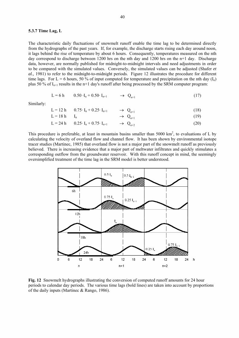
40

5.3.7 Time Lag, L

time lag to be determined directly from the hydrographs of the past years. If, for example, the discharge starts rising each day around noon,

erature by about 6 hours. Consequently, temperatures measured on the nth etween 1200 hrs on the nth day and 1200 hrs on the n+1 day. Discharge

in order et nt n)

n+1

L = 6 h 0.50 In + 0.50 In+1 → Qn+1 (17)

Similarly: L = 12 h 0.75. In + 0.2

L = 18 h In → Qn+1 (19) L = 24 h 0.25. In + 0.75. In+1 → Qn+2 (20)

in basins smaller than 5000 km2, to evaluations of L by nnel flow. It has been shown by environmental isotope

off as previously eltwater infiltrates and quickly stimulates a

orresponding outflow from the groundwater reservoir. With this runoff concept in mind, the seemingly

The characteristic daily fluctuations of snowmelt runoff enable the

it lags behind the rise of tempday correspond to discharge bdata, however, are normally published for midnight-to-midnight intervals and need adjustments to be compared with the simulated values. Conversely, the simulated values can be adjusted (Shafer al., 1981) to refer to the midnight-to-midnight periods. Figure 12 illustrates the procedure for differetime lags. For L = 6 hours, 50 % of input computed for temperature and precipitation on the nth day (I

lus 50 % of I results in the n+1 day's runoff after being processed by the SRM computer program: p

. .

5. In+1 → Qn+1 (18)

This procedure is preferable, at least in mountacalculating the velocity of overland flow and chatracer studies (Martinec, 1985) that overland flow is not a major part of the snowmelt runbelieved. There is increasing evidence that a major part of mcoversimplified treatment of the time lag in the SRM model is better understood.

Fig. 12 Snowmelt hydrographs illustrating the conversion of computed runoff amounts for 24 hour periods to calendar day periods. The various time lags (bold lines) are taken into account by proportions of the daily inputs (Martinec & Rango, 1986).

41

If the hydrographs are not available, or if their shape is distorted by reservoir operations, the time lag can be estimated according to the basin size and by analogy with other comparable basins. Generally, the time lag in a basin increases as the snow line retreats.

the WMO intercomparison test (WMOresults appear to be of little help to determine the proper values. Contradictory time lags have been calibrated by different models. However, if the time lags for all models participating in the WMO

parison test are averaged for each basin, the resulting values support the expected relation

Basin W-3 (8.42 kmDischma 7.2 h

If is some uncertainty, L (percentages in Equations (17)-(20)) can be adjusted in order to improve e synchronization of the simulated and measured peaks of average daily flows. It should be noted that a

In , 1986), most models calibrated the time lag. However, these

intercombetween L and basin size:

) : (43.3 km

2 3.0 h 2) :

Dunajec (680 km2) : 10.5 h Durance (2170 km2) : 12.4 h

there thsimilar effect results from an adjustment of the recession coefficient.

42

2, and the

6 ASSESSMENT OF THE MODEL ACCURACY

6.1 Accuracy criteria

The SRM computer program includes a graphical display of the computed hydrograph and of the measured runoff. A visual inspection shows at first glance whether the simulation is successful or not.

RM uses two well established accuracy criteria; namely, the coefficient of determination, RSvolume difference, Dv for a more objective assessment of how well the simulation has been carried out. The coefficient of determination is computed as follows:

R = 1(Q Q )

(Q Q)

2i i

'

i=1

2

i2

i=1

n−−

−

∑

∑ (21)

here: Qi

n

is the measured daily discharge w Qi

' is the computed daily discharge Q is the average measured discharge of the given year or snowmelt season n is the number of daily discharge values Equation (21) also corresponds to the Nash-Sutcliffe coefficient in which case Q is a long-term average

easured discharge applied to the respective years or seasons. The deviation of the runoff volumes, Dv,

mis computed as follows:

D [%] = V - V v

'

R

where: is the measured yearly or seasonal runoff volume s the co yearl sonal r olume Numerical accuracy criteria are never perfect, as illustrated by Figure 13. From the visual judgment both simula good b e the fu tal dif betwe extre s is w oduced. However, R2 to 0.48 in 1977. In spite of this unfavorable value, the simulation (or forecast) in 1977 would certainly be for wa nagem ause i tly reveals an extremely low runoff. For th with

V

R R 100⋅ (22)

VR

V' i mputed y or sea unoff vR

tions look ecaus ndamen ference en two me year ell repr = 0.95 in 1979 while it amounts only

useful ter ma ent bec t correc

Q ase year 1977, a long erage ted in ation ash-Su instead of the average for the specific year, a more favorable (but deceptive) value for R2 (0.97) is realized. This value is high because the long-term

-term av substitu to Equ (21) (N tcliffe) much

Q is much higher than any Q in 1977. Consequently, the daily deviations of the simula noff be elative nifican ough i te ter are not

egligible.

addition to these criteria which are automatically computed and displayed after each model run, the daily means, DG, could be computed by the user as follows:

ted ru come r ly insig t alth n absolu ms theyn Incoefficient of gain from

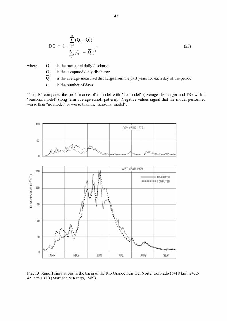
43

DG = 1(Q Q )

i ii 1

i i2

n−−

=

∑ (23)

(Q Q ) 'n

2

i=1

−∑

here: is the measured daily discharge is the computed daily discharge

Qi wQi

' Qi is the average measured discharge from the past years for each day of the period

is the number of days Thus, R2 compares the performance of a model with "no model" (average discharge) and DG with a "seasonal model" (long term average runoff pattern). Negative values signal that the model performed worse than "no model" or worse than the "seasonal model".

n

Fig. 13 Runoff simulations in the basin of the Rio Grande near Del Norte, Colorado (3419 km2, 2432-4215 m a.s.l.) (Martinec & Rango, 1989).

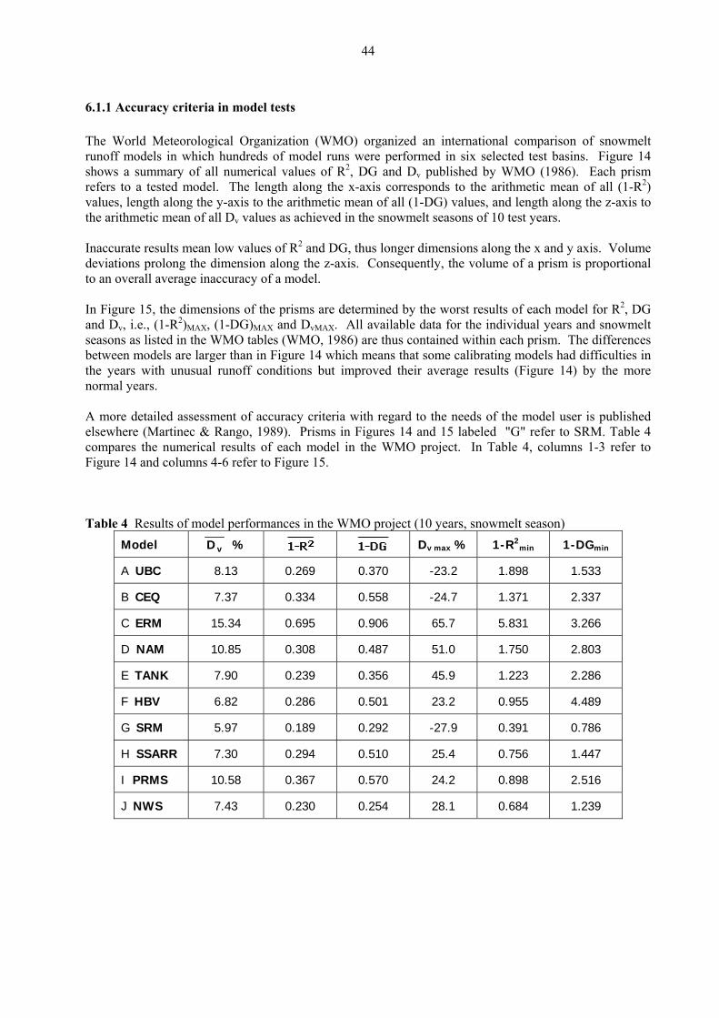
44

6.1.1 Accuracy criteria in model tests The World Meteorological Organization (WMO) organized an international comparison of snowmelt runoff models in which hundreds of model runs were performed in six selected test basins. Figure 14 shows a summary of all numerical values of R2, DG and Dv published by WMO (1986). Each prism refers to a tested model. The length along the x-axis corresponds to the arithmetic mean of all (1-R2) values, length along the y-axis to the arithmetic mean of all (1-DG) values, and length along the z-axis to the arithmetic mean of all Dv values as achieved in the snowmelt seasons of 10 test years. Inaccurate results mean low values of R2 and DG, thus longer dimensions along the x and y axis. Volume deviations prolong the dimension along the z-axis. Consequently, the volume of a prism is proportional to an overall average inaccuracy of a model. In Figure 15, the dimensions of the prisms are determined by the worst results of each model for R2, DG and Dv, i.e., (1-R2)MAX, (1-DG)MAX and DvMAX. All available data for the individual years and snowmelt seasons as listed in the WMO tables (WMO, 1986) are thus contained within each prism. The differences between models are larger than in Figure 14 which means that some calibrating models had difficulties in the years with unusual runoff conditions but improved their average results (Figure 14) by the more normal years. A more detailed assessment of accuracy criteria with regard to the needs of the model user is published elsewhere (Martinec & Rango, 1989). Prisms in Figures 14 and 15 labeled "G" refer to SRM. Table 4 compares the numerical results of each model in the WMO project. In Table 4, columns 1-3 refer to Figure 14 and columns 4-6 refer to Figure 15. Table 4 Results of model performances in the WMO project (10 years, snowmelt season)

Model %Dv Dv max % 1-R2min 1-DGmin

A UBC 8.13 0.269 0.370 -23.2 1.898 1.533

B CEQ 7.37 0.334 0.558 -24.7 1.371 2.337

C ERM 15.34 0.695 0.906 65.7 5.831 3.266

D NAM 10.85 0.308 0.487 51.0 1.750 2.803

E TANK 7.90 0.239 0.356 45.9 1.223 2.286

F HBV 6.82 0.286 0.501 23.2 0.955 4.489

G SRM 5.97 0.189 0.292 -27.9 0.391 0.786

H SSARR 7.30 0.294 0.510 25.4 0.756 1.447

I PRMS 10.58 0.367 0.570 24.2 0.898 2.516

J NWS 7.43 0.230 0.254 28.1 0.684 1.239

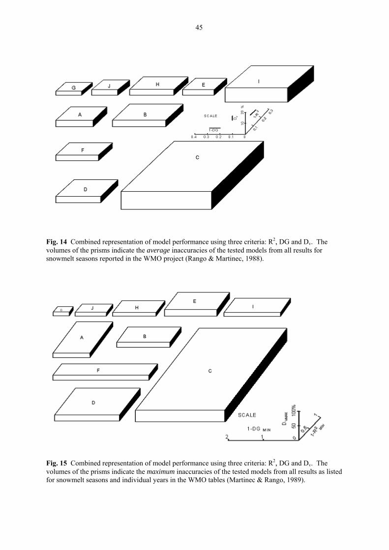
45

Fig. 14 Combined representation of model performance using three criteria: R2, DG and Dv. The v urasnow Ra

olumes of the prisms indicate the average inaccmelt seasons reported in the WMO project (

cies of the tested models from all results for ngo & Martinec, 1988).

Fig. 15 Combined representation of model performance using three criteria: R2, DG and Dv. The volumes of the prisms indicate the maximum inaccuracies of the tested models from all results as listed for snowmelt seasons and individual years in the WMO tables (Martinec & Rango, 1989).

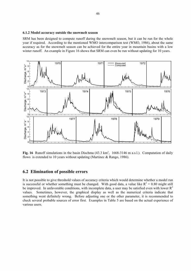
46

6 so

SRM has been designed to compute runoff during e year if required. According to the mentioned WM e accuracy as for the snowmelt season can be achievwinter runoff. An example in Figure 16 shows that

.1.2 Model accuracy outside the snowmelt sea n

the snowmelt season, but it can be run for the wholO intercomparison test (WMO, 1986), about the samed for the entire year in mountain basins with a low SRM can even be run without updating for 10 years.

F schma ( 2

f ting (Ma

6

It is not possible to give threshold values of accurac n is successful or whether something must be changed. With good data, a value like R2 = 0.80 might still be improved. In unfavorable conditions, with incomplete data, a user may be satisfied even with lower R2 v dispsom justincheck several probab e sources of error first. Exam ctual exp rience of

ig. 16 Runoff simulations in the basin Dilows is extended to 10 years without upda

43.3 km , 1668-3146 m a.s.l.). Computation of daily rtinec & Rango, 1986).

.2 Elimination of possible errors

y criteria which would determine whether a model ru

alues. Sometimes, however, the graphical ething went definitely wrong. Before ad

l

lay as well as the numerical criteria indicate that g one or the other parameter, it is recommended to ples in Table 5 are based on the a e

various users.

47

Table 5 Errors experienced by SRM users and their correction.

Error: Cause: 1 Runoff simulation went too high (Dinwoody,

1976, Dischma, 1977). Snow cover depletion curves distorted by summer snowfall (see Figure 5): Eliminate satellite observation after a snowfall event and redraw the depletion curves.

2 Runoff simulation suddenly deteriorated (Dischma).

t Input of snow coverage data S shifted by 1 month: Correcthe S-input.

3 The simulated runoff hydrograph declined uncontrollably in September (Illecillewaet basin).

Input of snow coverage data broken off by the end of August: Complete the S-input.

4 Runoff simulation far below the measured runoff (Illecillewaet).

Decimal point in the measured precipitation and discharge data shifted and thereby increasing the measured runoff 10x, but the simulated runoff only slightly: Correct the decimal point.

5 After the start of snowmelt, the simulated runoff (small

Values x, y for the recession coefficient formula (Equation k

,

kept decreasing in spite of snowmelt inputtributary basins of upper Rhine, 1985).

(7)) were taken over from a much larger basin so that exceeded 1.0 for low Q: Correct x, y with regard to the basin size. Possibility of this error was eliminated in thecomputer program Version 2.01 and later versions (3.0, 3.13.11, and 4.0).

6 ated

the measured runoff was influenced by storage (on weekends) and release from artificial reservoirs for hydropower. These interventions must be corrected in order to compare simulated and measured runoff.

Frequent deviations from the measured runoff, periodical lows of the hydrograph not simul(Felsberg 1982).

SRM simulates natural runoff while

7 Rainfall peaks inadequately simulated (Illecillewaet).

Rainfall input is concentrated to shorter periods than snowmelt input which accelerates the basin response. Program Versions 2.01 and later versions take this feature automatically into account whenever rainfall exceeds a preselected threshold.

8 Rainfall peak inadequately simulated even with the special rainfall peak program (small tributary basins of upper Rhine 25 August 1985).

Temperature extrapolated from station 800 m a.s.l. to zone D 2380 m a.s.l. by 0.65°C/100 m → T = + 0.43°C while TCRIT is + 0.75°C. By decreasing TCRIT, snowfall was converted to rainfall and the runoff peak was better simulated.

9 Rainfall peak inadequately simulated because the daily amount was below the special program automatic threshold. Threshold was lowered but the peak simulation deteriorated further. (small tributary basins of upper Rhine, 1985).

Only 1 precipitation station was available but the "by zone" option was switched on. Consequently precipitation input took place only in 1 zone. With 1 station, select option "basin wide".

48

Table 5 (cont.)

10 Runoff simulation went very high in a basin with Compact snow cover was assumed above the snow line so a large elevation range of 7400 m. (Kabul River, that the snow covered area was exaggerated. Temperature 1976). was extrapolated by too low a lapse rate. Snowmelt was

not computed separately for elevation zones but for the entire basin. This usually leads to overestimation of meltwater input. Simulation was improved by re-evaluating the snow coverage and selecting a higher temperature lapse rate corresponding to the climate. With regard to the large elevation range, the basin should have been divided in several elevation zones.

11 Distorted runoff simulation (outflow from a snow lysimeter).

Values of recession coefficient false: Negative y values used with the equation k = x.Q-y so that the exponent became positive. Consequently, k increased with the increasing Q while it should have decreased. Use equation k = x.Q-y and positive values of y, so that the exponent is always negative.

12 Difficulties with the timing of rainfall-runoff peaks (WMO test for simulated operational forecasts, Illecillewaet basin).

Precipitation data from one of the stations were ascribed to the date on which it was measured at 0800. Data had to be shifted one day backwards. See also Section 5.2.2.

13 Forecasted runoff for hydroelectric stations Sedrun and Tavanasa too low in April-June

Snte

1994. In one run, snow cover was not

owmelt was computed by smooth long term average mperature thus decreasing the number of degree days.

Reintroduce the daily fluctuations of temperatures. completely melted by the end of September.

14 Discrepancies in runoff simulations for Rio Grande near Del Norte.

Erratic precipitation data. Automatic extrapolation by altitude gradients from two stations resulted in negative precipitation amounts in the highest zone when gradient was negative. Extrapolate averaged precipitation data by a uniform gradient as recommended in Section 5.2. Always visually inspect input precipitation data.

15 Discrepancies in runoff simulations for Rio Grande near Del Norte

Occasionally missing temperature data were interpreted by the computer program as 0 = 0°C. Inspect temperature data and complete missing values by interpolation.

16 Effect of climate change (see Section 8.3): Decrease of runoff computed by an increased temperature (Rio Grande near Del Norte)

The "winter deficit" was exceeded on a warm day with a high snowmelt depth, so that too much was cut off from MDCEXCL. Consequently CDCCLIM was shifted too much and less runoff resulted. Cut off MDCEXCL by the value of the previous day ("nearly equaled").

17 Overestimation of runoff in the Rhine-Felsberg basin 1-15 May 1993 with usual temperature lapse rate of 0.65°C/100 m.

Frequent föhn-wind in this period, temperature differences between Weissfluhjoch ( 2693 m a.s.l.) and Davos (1560 m a.s.l.) correspond to a lapse rate as high as 0.95°C/100 m. The value of 0.8°C/100 m was used.

49

Table 5 (cont.)

C zone (1700-2300 m.a.s.l.) but still exists in precipitation and snowmelt depths in winter in each zone (Figs. 25, 26). The snow in the B zone was completely melted for T oC on 1 April so that no winter deficit resulted

and therefore the existing o

ever satellites see some snow on 1 April and the winter accumulation of snow from precipitation and

18 Evaluation of the climate effect in the Kings River basin 1973: For a temperature increase +4oC, snow cover on 1 April disappears in the

The decrease of the snow water equivalent on 1 April due to warming is evaluated from uniform amounts of

the lower B zone (1100-1700 m.a.s.l.) for T+4o. However, in reality, some snow survived for T oC due to variable snow depths as seen by satellites (S=27% on 1 April). With no computed snow for T oC as well as for T+4o, no winter deficit resultedsnow cover was falsely preserved for T+4 . A manual correction (elimination of CDCCLIM) was necessary. In the C zone there was enough snow to avoid the error from uniform, instead of variable, snow depths in winter, so that the snow cover duly disappeared as a result of the evaluated winter deficit. This error can occur only with very little snow in a zone on 1 April and can be readily corrected. When

snowmelt is zero, eliminate CDCCLIM.

19 Failure of runoff simulations in the basin Pskem: the derived constant y in the recession formula (Eq. 7) is negative, so that the recession is steeper for low flows than for high flows. The envelope line in Fig. 10 was derived taking into account evidently false points in the

The recession of the natural runoff slows down with a decreasing discharge. To this effect, y must be > 0. In a log-log representation (Fig. 10), the points outside the range between the 1:1 line and a parallel line for points in the range of high flows (below the dashed line in Fig. 10) must be disregarded. With this measure, the prob

low range of flows. Such points may occur, for lem of the

runoff simulation was eliminated. example, when the river flow is artificially stopped by freezing.

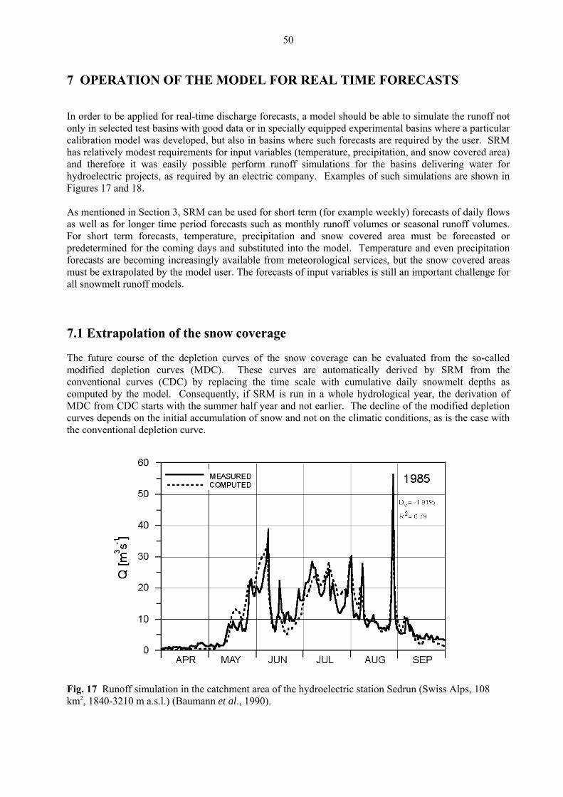
50

7 OPERATION OF THE MODEL FOR REAL TIME FORECASTS

In order to be applied for real-time discharge forecasts, a model should be able to simulate the runoff not only in selected test basins with good data or in specially equipped experimental basins where a particular calibration model was developed, but also in basins where such forecasts are required by the user. SRM has relatively modest requirements for input variables (temperature, precipitation, and snow covered area) and therefore it was easily possible perform runoff simulations for the basins delivering water for hydroelectric projects, as required by an electric company. Examples of such simulations are shown in Figures 17 and 18. As mentioned in Section 3, SRM can be used for short term (for example weekly) forecasts of daily flows as well as for longer time period forecasts such as monthly runoff volumes or seasonal runoff volumes. For short term forecasts, temperature, precipitation and snow covered area must be forecasted or predetermined for the coming days and substituted into the model. Temperature and even precipitation forecasts are becoming increasingly available from meteorological services, but the snow covered areas must be extrapolated by the model user. The forecasts of input variables is still an important challenge for all snowmelt runoff models.

.1 Extrapolation of the snow coverage

ese curves are automatically derived by SRM from the onventional curves (CDC) by replacing the time scale with cumulative daily snowmelt depths as omputed by the model. Consequently, if SRM is run in a whole hydrological year, the derivation of

MDC from CDC starts with the summer half year and not earlier. The decline of the modified depletion urves depends on the initial accumulation of snow and not on the climatic conditions, as is the case with

7

The future course of the depletion curves of the snow coverage can be evaluated from the so-called modified depletion curves (MDC). Thcc

cthe conventional depletion curve.

Fig. 17 Runoff simulation in the catchment area of the hydroelectric station Sedrun (Swiss Alps, 108 km2, 1840-3210 m a.s.l.) (Baumann et al., 1990).

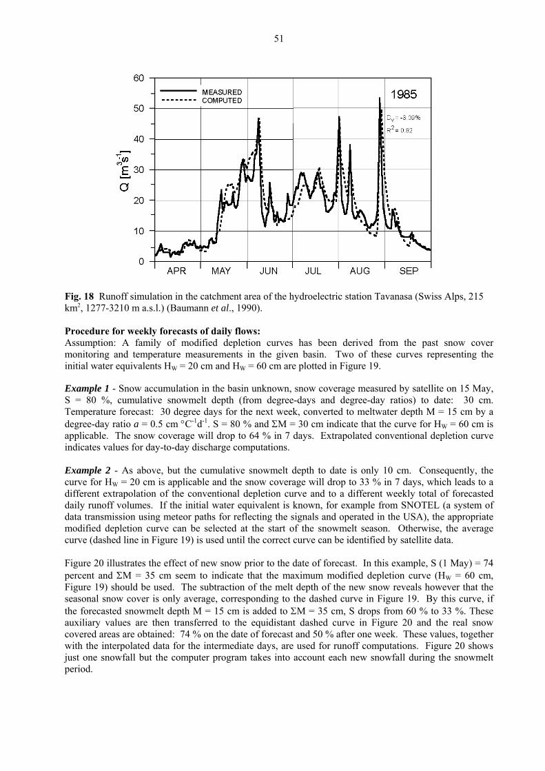
51

Fig. 18 Runoff simulation in the catchment area of the hydroelectric station Tavanasa (Swiss Alps, 215 km2, 1277-3210 m a.s.l.) (Baumann et al., 1990). Procedure for weekly forecasts of daily flows: Assumption: A family of modified depletion curves has been derived from the past snow cover monitoring and temperature measurements in the given basin. Two of these curves representing the initial water equivalents HW = 20 cm and HW = 60 cm are plotted in Figure 19.

he average

19. By this curve, if the forecasted snowmelt depth M = 15 cm is added to ΣM = 35 cm, S drops from 60 % to 33 %. These auxiliary values are then transferred to the equidistant dashed curve in Figure 20 and the real snow covered areas are obtained: 74 % on the date of forecast and 50 % after one week. These values, together with the interpolated data for the intermediate days, are used for runoff computations. Figure 20 shows just one snowfall but the computer program takes into account each new snowfall during the snowmelt period.

Example 1 - Snow accumulation in the basin unknown, snow coverage measured by satellite on 15 May, S = 80 %, cumulative snowmelt depth (from degree-days and degree-day ratios) to date: 30 cm. Temperature forecast: 30 degree days for the next week, converted to meltwater depth M = 15 cm by a degree-day ratio a = 0.5 cm °C-1d-1. S = 80 % and ΣM = 30 cm indicate that the curve for HW = 60 cm is applicable. The snow coverage will drop to 64 % in 7 days. Extrapolated conventional depletion curve indicates values for day-to-day discharge computations. Example 2 - As above, but the cumulative snowmelt depth to date is only 10 cm. Consequently, the curve for HW = 20 cm is applicable and the snow coverage will drop to 33 % in 7 days, which leads to a different extrapolation of the conventional depletion curve and to a different weekly total of forecasted daily runoff volumes. If the initial water equivalent is known, for example from SNOTEL (a system of data transmission using meteor paths for reflecting the signals and operated in the USA), the appropriate modified depletion curve can be selected at the start of the snowmelt season. Otherwise, tcurve (dashed line in Figure 19) is used until the correct curve can be identified by satellite data. Figure 20 illustrates the effect of new snow prior to the date of forecast. In this example, S (1 May) = 74 percent and ΣM = 35 cm seem to indicate that the maximum modified depletion curve (HW = 60 cm, Figure 19) should be used. The subtraction of the melt depth of the new snow reveals however that the seasonal snow cover is only average, corresponding to the dashed curve in Figure

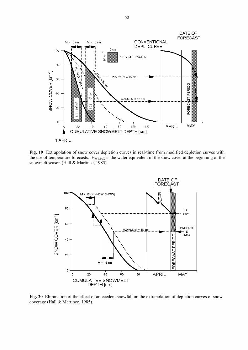
52

Fig. 19 Extrapolation of snow cover depletion curves in real-time from modified depletion curves with the use of temperature forecasts. HW MAX is the water equivalent of the snow cover at the beginning of the snowmelt season (Hall & Martinec, 1985).

Fig. 20 Elimination of the effect of antecedent snowfall on the extrapolation of depletion curves of snow coverage (Hall & Martinec, 1985).

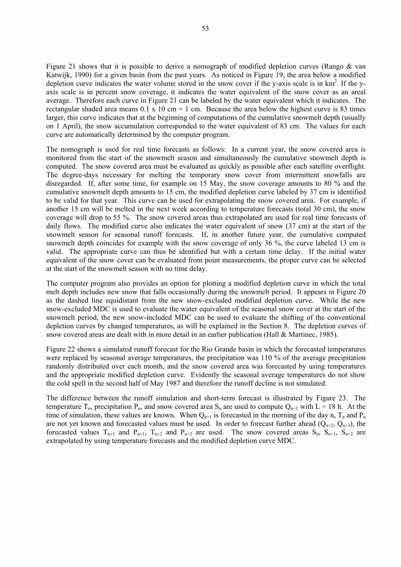
53

Figure 21 shows that it is possible to derive a nomograph of modified depletion curves (Rango & van Katwijk, 1990) for a given basin from the past years. As noticed in Figure 19, the area below a modified depletion curve indicates the water volume stored in the snow cover if the y-axis scale is in km2. If the y-axis scale is in percent snow coverage, it indicates the water equivalent of the snow cover as an areal average. Therefore each curve in Figure 21 can be labeled by the water equivalent which it indicates. The rectangular shaded area means 0.1 x 10 cm = 1 cm. Because the area below the highest curve is 83 times larger, this curve indicates that at the beginning of computations of the cumulative snowmelt depth (usually on 1 April), the snow accumulation corresponded to the water equivalent of 83 cm. The values for each curve are automatically determined by the computer program. The nomograph is used for real time forecasts as follows: In a current year, the snow covered area is monitored from the start of the snowmelt season and simultaneously the cumulative snowmelt depth is computed. The snow covered area must be evaluated as quickly as possible after each satellite overflight. The degree-days necessary for melting the temporary snow cover from intermittent snowfalls are disregarded. If, after some time, for example on 15 May, the snow coverage amounts to 80 % and the cumulative snowmelt depth amounts to 15 cm, the modified depletion curve labeled by 37 cm is identified to be valid for that year. This curve can be used for extrapolating the snow covered area. For example, if another 15 cm will be melted in the next week according to temperature forecasts (total 30 cm), the snow coverage will drop to 55 %. The snow covered areas thus extrapolated are used for real time forecasts of daily flows. The modified curve also indicates the water equivalent of snow (37 cm) at the start of the snowmelt season for seasonal runoff forecasts. If, in another future year, the cumulative computed

owmelt depth coincides for example with the snow coverage of only 36 %, the curve labeled 13 cm is ater

an be evaluated from point measurements, the proper curve can be selected the start of the snowmelt season with no time delay.

to evaluate the water equivalent of the seasonal snow cover at the start of the owmelt period, the new snow-included MDC can be used to evaluate the shifting of the conventional

peratures

recast is illustrated by Figure 23. The

t yet known and forecasted values must be used. In order to forecast further ahead (Qn+2, Qn+3), the n+1 and Pn+1, Tn+2 and Pn+2 are used. The snow covered areas Sn, Sn+1, Sn+2 are g temperature forecasts and the modified depletion curve MDC.

snvalid. The appropriate curve can thus be identified but with a certain time delay. If the initial wequivalent of the snow cover cat The computer program also provides an option for plotting a modified depletion curve in which the total melt depth includes new snow that falls occasionally during the snowmelt period. It appears in Figure 20 as the dashed line equidistant from the new snow-excluded modified depletion curve. While the new snow-excluded MDC is used sndepletion curves by changed temperatures, as will be explained in the Section 8. The depletion curves of snow covered areas are dealt with in more detail in an earlier publication (Hall & Martinec, 1985).

gure 22 shows a simulated runoff forecast for the Rio Grande basin in which the forecasted temFiwere replaced by seasonal average temperatures, the precipitation was 110 % of the average precipitation randomly distributed over each month, and the snow covered area was forecasted by using temperatures and the appropriate modified depletion curve. Evidently the seasonal average temperatures do not show the cold spell in the second half of May 1987 and therefore the runoff decline is not simulated. The difference between the runoff simulation and short-term fotemperature Tn, precipitation Pn, and snow covered area Sn are used to compute Qn+1 with L = 18 h. At the time of simulation, these values are known. When Qn+1 is forecasted in the morning of the day n, Tn and Pn are noforecasted values Textrapolated by usin

54

ig. 21 Nomograph of modified depletion curves for the elevation zone B (1284 km2, 2926-3353 m a.s.l.) ge water

equivalent (1 April) of the snow cover which they represent (Rango & van Katwijk 1990).

Fof the Rio Grande basin near Del Norte, Colorado. The curves are labeled with the areal avera

Fig. 22 Simulated real-time runoff forecast for the Rio Grande basin using long-term average temperatures instead of temperatures for the year 1983 (Rango & van Katwijk, 1990).

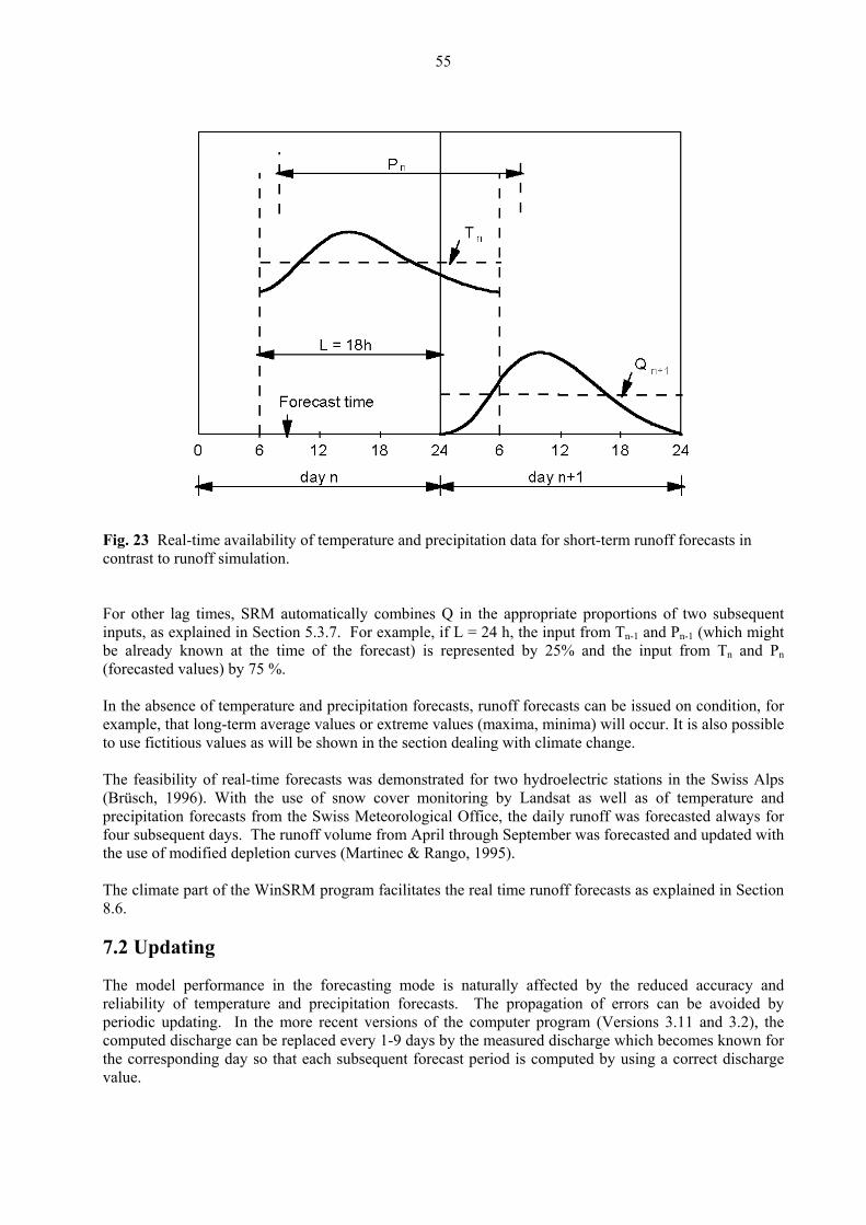
55

F . of temperature and precipitation data for short-term runoff forecasts in c tr . F atically combines Q in the appropriate proportions of two subsequent inputs, ple, if L = 24 h, the input from Tn-1 and Pn-1 (which might be already known at the time of the forecast) is represented by 25% and the input from Tn and Pn

ber was forecasted and updated with e use of modified depletion curves (Martinec & Rango, 1995).

asts as explained in Section

ram (Versions 3.11 and 3.2), the es known for

the corresponding day so that each subsequent forecast period is computed by using a correct discharge value.

ig 23 Real-time availabilityon ast to runoff simulation

or other lag times, SRM automas explained in Section 5.3.7. For exam

(forecasted values) by 75 %. In the absence of temperature and precipitation forecasts, runoff forecasts can be issued on condition, for example, that long-term average values or extreme values (maxima, minima) will occur. It is also possible to use fictitious values as will be shown in the section dealing with climate change. The feasibility of real-time forecasts was demonstrated for two hydroelectric stations in the Swiss Alps (Brüsch, 1996). With the use of snow cover monitoring by Landsat as well as of temperature and precipitation forecasts from the Swiss Meteorological Office, the daily runoff was forecasted always for

ur subsequent days. The runoff volume from April through Septemfoth The climate part of the WinSRM program facilitates the real time runoff forec8.6.

7.2 Updating

The model performance in the forecasting mode is naturally affected by the reduced accuracy and reliability of temperature and precipitation forecasts. The propagation of errors can be avoided by periodic updating. In the more recent versions of the computer progcomputed discharge can be replaced every 1-9 days by the measured discharge which becom

56

2Fig. 24 Discharge simulation in the Dinwoody Creek basin (228 km , 1981-4202 m a.s.l.) in Wyoming,

ature which efficient if Equation (7) is carefully assessed: Figure 24a shows a model runoff simulation starting with omputed discharge of only one half of the correct value. Updating by actual discharge improves the

simulation as shown in Figure 24b. Even without updating, however, the initial discrepancy is soon eliminated automatically.

Further possibilities of updating will be made available to users when more experience in real time tuations is accumulated. For example, it should be possible to adjust some parameters (e.g., the runoff oefficient) in the progress of the forecast, but only within hydrologically and physically acceptable

data is indicated.

(1) Updating the computed discharge by the measured discharge when it becomes known,

(3) Correction of temperature, precipitation, and snow cover forecasts according to actual observations.

Short-term discharge forecasts can be updated as frequently as each day (Baumann et al., 1990).

(a) without updating, and (b) with updating by actual discharge on 1 August. Even without this updating, SRM prevents persistent large errors by a built-in self adjusting feisc

siclimits. In any case, false forecasts of temperature and precipitation should be updated whenever a correction by new What is generally called "updating" can be thus divided into 3 categories:

i.e., checking with the measured discharge to avoid carry-over of errors when the next forecast is issued.

(2) Adjustment of model parameters in the process of forecast.

57

8 YEAR-ROUND RUNOFF SIMULATION FOR A CHANGED CLIMATE

SRM uses a real snow cover from satellite monitoring in the present climate in order to produce a snow over and runoff in a changed climate. This requiresc a rather detailed procedure, but uncertainties arising

esults and hydrographs, within minutes. Another advantage is the independence from alibration, enabling the model parameters to be meaningfully shifted in time or adjusted if so indicated y climate scenarios.

o predict snow covered areas and regional snow accumulation in a changed climate, ple, in m drologically defined basins, the computer program

requires the following data:

• Number of elevation zones, their areas, and hypsometric mean elevations

• Current snow covered areas, daily values (S)

ily average or Max/Min temperatures (T)

• Precipitation, daily (P)

• De

• Temperature lapse rate (γ)

• Cr

For runoff computation, the remaining SRM parameters are required: cS cR, RCA, k, L and the initial Q.

riginally, SRM was applied to simulate and forecast runoff only during the snowmelt season. It was later ru MO, 1986). The first evaluation of

e effect of climate change of SRM dates back to 1980 (Martinec, 1980). At that time there was no consens refore, the runoff in the snowmelt season was computed for +1oC and –1oC. Since then, climate scenarios anticipating increasing tempera year. Consequently, the SRM climate program has been extended to handle the winter half year as well.

8.1 Snowmelt runoff computation in the winter half year

ion of the snow overage is more difficult than during the snowmelt season, because of persistent cloudiness and low sun

om cover

s may lead to an overestimation of the snow coverage. Two ptions are available to handle this problem during the winter months:

from a fictitious snow cover simulated from precipitation and arbitrary threshold temperatures are avoided. In any event, the SRM program finishes this task, including printout of figures, tables,

umerical rncb If SRM is used only tfor exam ountain areas which are not hy

• Da

factor (a) gree-day

itical temperature (TCRIT)

On year-round for international tests of model performance (W

thus yet whether temperature will increase or decrease. The

tures have become available for the whole

In the winter half year (usually October-March in the Northern hemisphere), the evaluatcangles. Satellite data, if available, are not frequent enough to distinguish the stable snow cover frfrequent transitory snowfalls which are subsequently melted. An assumption of a stable snow between two available satellite measuremento

58

Option 1: Put S = 0 so that each precipitation event recognized by TCRIT as snow is automatically stored and subsequently melted over the whole area (1 - S = 1). This method is applicable only if precipitation data are good enough to represent the input or if they can be adequately adjusted.

zones while in the lowest zone option 1 may be preferable. The present program keeps the snow coverage estimated for the present climate unchanged for climate runs. It is therefore recommended to assume a complete snow coverage only in months in which it is expected to last in a warmer climate as well.

henever S = 1 is introduced, the SRM program cancels any existing storage of preceding temporary owfalls because such snow becomes a part of the seasonal snow cover. Snow storage is also

be adapted to winter conditions. In particular, the constants x, y for the recession formula (Equation (7)) derived usually for summer conditions sometimes allow the discharge to decrease too low so that a slower recession formula is indicated. By using the Equation (14):

This is in many cases not possible due to the well known catch deficit of precipitation gauges and due to the lack of measurements in the high elevations of mountain regions. It is for this reason that SRM uses the snow covered area whenever possible for computing the runoff input. Option 2: Assume a stable snow cover (S = 1 or a little less in a rugged terrain) in January and February, for example, and S = 0 in October - December. If S = 1 on 1 April from satellite data, assume S = 1 in March as well. If it is less than 1 on 1 April, the snow coverage in March is put to 0 or, which may be more accurate, it is interpolated from 1 on 1 March to the S-value on 1 April. Naturally, S = 1 can be assumed for a longer part of the winter in higher elevation

Wsnautomatically canceled on the 1 April date because all existing snow is then accounted for by the depletion curve of the seasonal snow coverage. With the variables thus accounted for, SRM is run as usual. Because the estimated snow coverage is less accurate than measured CDC in the summer, the water equivalent of new snow is reduced at once by the simultaneous (1 - S) to prevent an inadequate S from influencing the computation on a later melt day. This deviates from the summer procedure explained in Section 5.2.2, Table 2. The model parameters should

Q > xMin

1y (14)

x, y can be adjusted in order to prevent the discharge from sinking below a selected level after a long recession period. In view of frequent snowfalls, values of the degree-day factor lower than those used in the summer are recommended. Values of cS and cR higher than in summer can be expected. The main purpose of the winter runoff simulation is the evaluation of the runoff redistribution between the winter and summer half years. Consequently, it is more important to compute the winter runoff volume as accurately as possible rather than to try to improve the daily accuracy (R2).

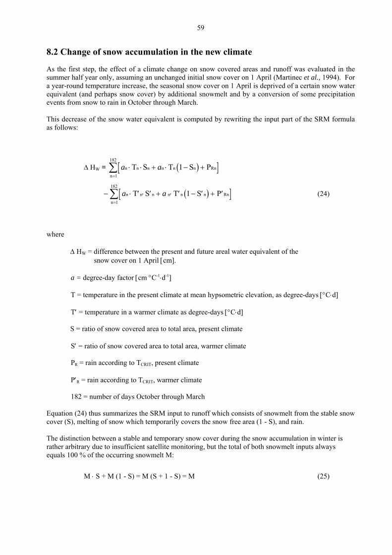
59

8.2 Change of snow accumulation in the new climate

s the first step, the effect of a climate change on snow covered areas and runoff was evaluated in the mmer half year only, assuming an unchanged initial snow cover on 1 April (Martinec et al., 1994). For

of a certain snow water ersion of some precipitation

events from snow to rain in October through March.

mula

Asua year-round temperature increase, the seasonal snow cover on 1 April is deprived equivalent (and perhaps snow cover) by additional snowmelt and by a conv

This decrease of the snow water equivalent is computed by rewriting the input part of the SRM foras follows:

∆ HW = ( )[ ]a an n n n n n Rn

n

T S T S P⋅ ⋅ + ⋅ − +=

∑ 11

182

( )[ ]− ⋅

where

sn

a = degre T = tempe T′ = temperature in a warmer climate as degree-days [°C⋅d]

S = ratio o

S′ = ratio PR = rain according to TCRIT, present climate

P′R = rain 182 = number of days October through March

Equation (24) thus cover (S), melting The distinction between a stable and temporary snow cover during the snow accumulation in winter is rather arbitraryequals 100 %

M ⋅ S + M (1 - S) = M (S + 1 - S) = M (25)

′ ⋅ ′ + ⋅ ′ − ′ + ′=

∑ a an n n n Rn

n

S T S PT n n 11

(24) 182

∆ HW = difference between the present and future areal water equivalent of the ow cover on 1 April [cm].

e-day factor [cm °C-1⋅d-1]

rature in the present climate at mean hypsometric elevation, as degree-days [°C⋅d]

f snow covered area to total area, present climate

of snow covered area to total area, warmer climate

according to TCRIT, warmer climate

summarizes the SRM input to runoff which consists of snowmelt from the stable snow of snow which temporarily covers the snow free area (1 - S), and rain.

due to insufficient satellite monitoring, but the total of both snowmelt inputs always of the occurring snowmelt M:

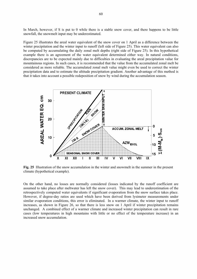
60

In March, howeve snowfall, the snow Figur winter precipitatio be computed by a l example there is discrepancies are precipitation value for mountainous regions. In such cases, it is recommended that the value from the accumulated zonal melt be consi precip that it takes into ac d during the accumulation season.

r, if S is put to 0 while there is a stable snow cover, and there happens to be littlemelt input may be underestimated.

e 25 illustrates the areal water equivalent of the snow cover on 1 April as a difference between then and the winter input to runoff (left side of Figure 25). This water equivalent can alsoccumulating the daily zonal melt depths (right side of Figure 25). In this hypotheticaan agreement of the water equivalent determined either way. In natural conditions,to be expected mainly due to difficulties in evaluating the areal

dered as more reliable. The accumulated zonal melt value might even be used to correct the winteritation data and to estimate the altitude precipitation gradient. Another advantage of this method is

count a possible redeposition of snow by win

Fig. 25 Illustration of the snow accumulation in the winter and snowmelt in the summer in the present

n in Figure 26, so that there is less snow on 1 April if winter precipitation remains nchanged. A combined effect of a warmer climate and increased winter precipitation can result in rare

case in an increase

climate (hypothetical example). On the other hand, no losses are normally considered (losses indicated by the runoff coefficient are assumed to take place after meltwater has left the snow cover). This may lead to underestimation of the retrospectively computed water equivalents if significant evaporation from the snow surface takes place. However, if degree-day ratios are used which have been derived from lysimeter measurements under similar evaporation conditions, this error is eliminated. In a warmer climate, the winter input to runoff increases, as showu

s (low temperatures in high mountains with little or no effect of the temperature increase) d snow accumulation.

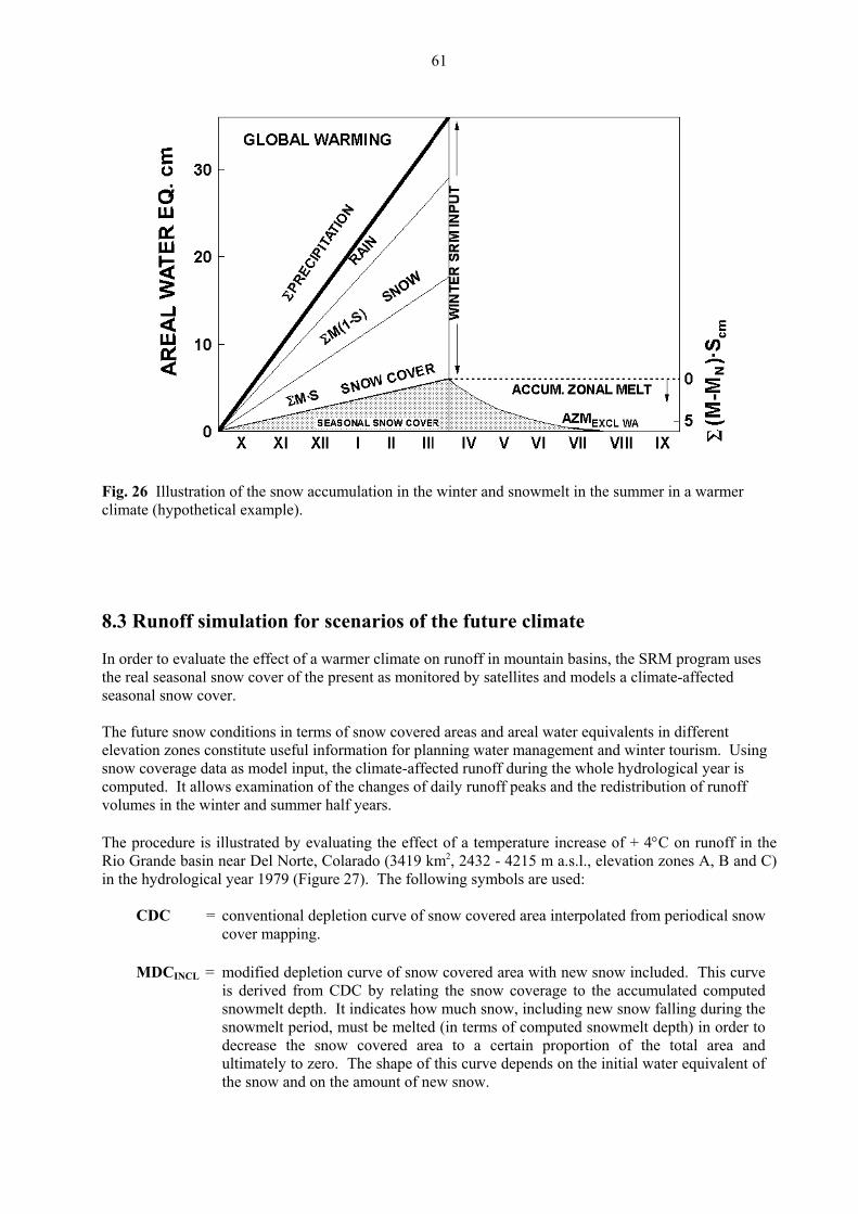
61

Illustration of the snow accumulation in the winter and snowmelt in the summer in a warmerhypothetical example).

Fig. 26 climate (

8.3 Ru

In order climate on runoff in mountain basins, the SRM program uses the seasonal The future snow conditions in termelev sing snow cov s compute f volumes The proc in the Rio Gran nd C) in the hy

CD now

MD urve uted the r to and t of

noff simulation for scenarios of the future climate

to evaluate the effect of a warmerreal seasonal snow cover of the present as monitored by satellites and models a climate-affected

snow cover.

s of snow covered areas and areal water equivalents in different ation zones constitute useful information for planning water management and winter tourism. U

erage data as model input, the climate-affected runoff during the whole hydrological year id. It allows examination of the changes of daily runoff peaks and the redistribution of runof in the winter and summer half years.

edure is illustrated by evaluating the effect of a temperature increase of + 4°C on runoff de basin near Del Norte, Colarado (3419 km2, 2432 - 4215 m a.s.l., elevation zones A, B adrological year 1979 (Figure 27). The following symbols are used:

C = conventional depletion curve of snow covered area interpolated from periodical scover mapping.

CINCL = modified depletion curve of snow covered area with new snow included. This cis derived from CDC by relating the snow coverage to the accumulated compsnowmelt depth. It indicates how much snow, including new snow falling duringsnowmelt period, must be melted (in terms of computed snowmelt depth) in ordedecrease the snow covered area to a certain proportion of the total area ultimately to zero. The shape of this curve depends on the initial water equivalenthe snow and on the amount of new snow.

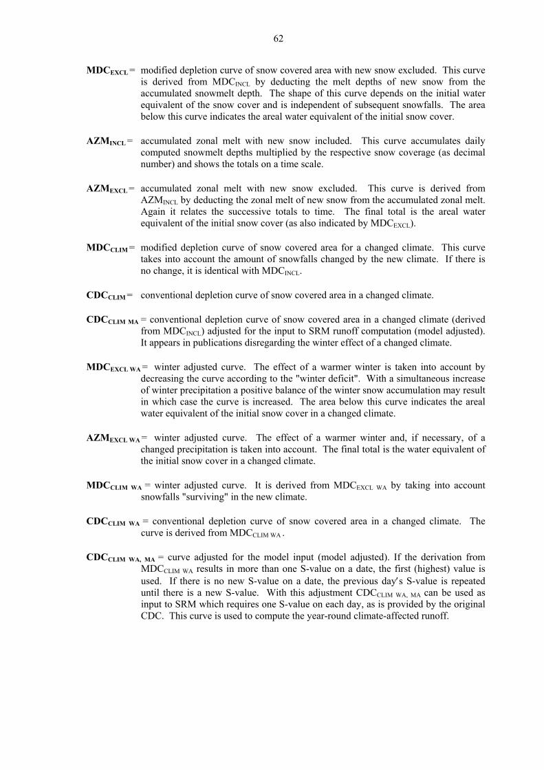
62

MD urve ting the melt depths of new snow from the

ac ater area

AZ INCL ulates daily computed snowmelt depths multiplied by the respective snow coverage (as decimal number) and shows the totals on a time scale.

AZMEXCL = accumulated zonal melt with new snow excluded. This curve is derived from AZMINCL by deducting the zonal melt of new snow from the accumulated zonal melt. Again it relates the successive totals to time. The final total is the areal water equivalent of the initial snow cover (as also indicated by MDCEXCL).

MDCCLIM = modified depletion curve of snow covered area for a changed climate. This curve takes into account the amount of snowfalls changed by the new climate. If there is no change, it is identical with MDCINCL.

CDCCLIM = conventional depletion curve of snow covered area in a changed climate.

CDCCLIM MA = conventional depletion curve of snow covered area in a changed climate (derived from MDCINCL) adjusted for the input to SRM runoff computation (model adjusted). It appears in publications disregarding the winter effect of a changed climate.

MDCEXCL WA = winter adjusted curve. The effect of a warmer winter is taken into account by decreasing the curve according to the "winter deficit". With a simultaneous increase of winter precipitation a positive balance of the winter snow accumulation may result in which case the curve is increased. The area below this curve indicates the areal water equivalent of the initial snow cover in a changed climate.

AZMEXCL WA = winter adjusted curve. The effect of a warmer winter and, if necessary, of a changed precipitation is taken into account. The final total is the water equivalent of the initial snow cover in a changed climate.

MDCCLIM WA = winter adjusted curve. It is derived from MDCEXCL WA by taking into account snowfalls "surviving" in the new climate.

CDCCLIM WA = conventional depletion curve of snow covered area in a changed climate. The curve is derived from MDCCLIM WA .

CDCCLIM WA, MA = curve adjusted for the model input (model adjusted). If the derivation from MDCCLIM WA results in more than one S-value on a date, the first (highest) value is used. If there is no new S-value on a date, the previous day′s S-value is repeated until there is a new S-value. With this adjustment CDCCLIM WA, MA can be used as input to SRM which requires one S-value on each day, as is provided by the original CDC. This curve is used to compute the year-round climate-affected runoff.

CEXCL = modified depletion curve of snow covered area with new snow excluded. This cis derived from MDCINCL by deduc

cumulated snowmelt depth. The shape of this curve depends on the initial wequivalent of the snow cover and is independent of subsequent snowfalls. The below this curve indicates the areal water equivalent of the initial snow cover.

M = accumulated zonal melt with new snow included. This curve accum

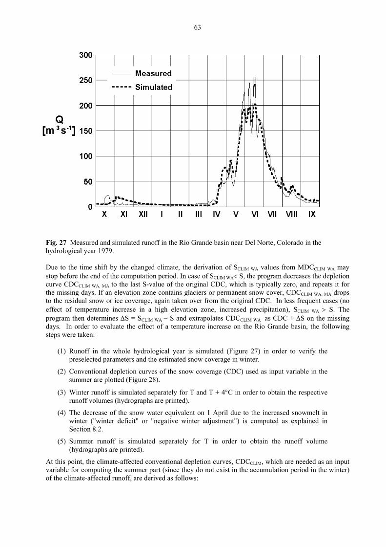
63

Fig. 27 Measured and simulated runoff in the Rio Grande basin near Del Norte, Colorado in the ydrological year 1979.

Due to the time shift by the changed climate, the derivation of SCLIM WA values from MDCCLIM WA may tion

or CLIM WA, MA

the residual snow or ice coverage, again taken over from the original CDC. In less frequent cases (no effect of temperature increase in a high elevation zone, increased precipitation), SCLIM WA > S. The program then determines ∆S = SCLIM WA − S and extrapolates CDCCLIM WA as CDC + ∆S on the missing days. In order to evaluate the effect of a temperature increase on the Rio Grande basin, the following steps were taken:

(1) Runoff in the whole hydrological year is simulated (Figure 27) in order to verify the preselected parameters and the estimated snow coverage in winter.

(2) Conventional depletion curves of the snow coverage (CDC) used as input variable in the summer are plotted (Figure 28).

(3) Winter runoff is simulated separately for T and T + 4°C in order to obtain the respective runoff volumes (hydrographs are printed).

(4) The decrease of the snow water equivalent on 1 April due to the increased snowmelt in winter ("winter deficit" or "negative winter adjustment") is computed as explained in Section 8.2.

(5) Summer runoff is simulated separately for T in order to obtain the runoff volume (hydrographs are printed).

At this point, the climate-affected conventional depletion curves, CDCCLIM, which are needed as an input variable for computing the summer part (since they do not exist in the accumulation period in the winter) of the climate-affected runoff, are derived as follows:

h

stop before the end of the computation period. In case of SCLIM WA< S, the program decreases the deplecurve CDCCLIM WA, MA to the last S-value of the original CDC, which is typically zero, and repeats it f

e missing days. If an elevation zone contains glaciers or permanent snow cover, CDC drops thto

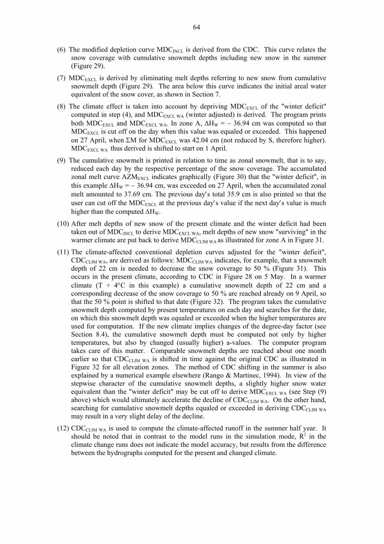
64

(6) The modified depletion curve MDCINCL is derived from the CDC. This curve relates the snow coverage with cumulative snowmelt depths including new snow in the summer (Figure 29).

(7) MDCEXCL is derived by eliminating melt depths referring to new snow from cumulative snowmelt depth (Figure 29). The area below this curve indicates the initial areal water equivalent of the snow cover, as shown in Section 7.

(8) The climate effect is taken into account by depriving MDCEXCL of the "winter deficit" computed in step (4), and MDCEXCL WA (winter adjusted) is derived. The program prints both MDCEXCL and MDCEXCL WA. In zone A, ∆HW = − 36.94 cm was computed so that MDCEXCL is cut off on the day when this value was equaled or exceeded. This happened on 27 April, when ΣM for MDCEXCL was 42.04 cm (not reduced by S, therefore higher). MDCEXCL WA thus derived is shifted to start on 1 April.

(9) The cumulative snowmelt is printed in relation to time as zonal snowmelt, that is to say, reduced each day by the respective percentage of the snow coverage. The accumulated zonal melt curve AZMEXCL indicates graphically (Figure 30) that the "winter deficit", in this example ∆HW = − 36.94 cm, was exceeded on 27 April, when the accumulated zonal melt amounted to 37.69 cm. The previous day′s total 35.9 cm is also printed so that the user can cut off the MDC at the previous day′s value if the next day′s value is much

INCL EXCL WA f new snow "surviving" in the warmer climate are put back to derive MDCCLIM WA as illustrated for zone A in Figure 31.

(11) The climate-affected conventional depletion curves adjusted for the "winter deficit", CDCCLIM WA, are derived as follows: MDCCLIM WA indicates, for example, that a snowmelt depth of 22 cm is needed to decrease the ow coverage to 50 % (Figure 31). This occurs in the present climate, according to CDC in Figure 28 on 5 May. In a warmer

hed already on 9 April, so that the 50 % point is shifted to that date (Figure 32). The program takes the cumulative snowmelt depth computed by present temperatures on each day and searches for the date, on which this snowmelt depth was equaled or exceeded when the higher temperatures are used for computation. If the new climate implies changes of the degree-day factor (see Section 8.4), the cumulative snowmelt depth must be computed not only by higher temperatures, but also by changed (usually higher) a-values. The computer program takes care of this matter. Comparable snowmelt depths are reached about one month earlier so that CDCCLIM WA is shifted in time against the original CDC as illustrated in Figure 32 for all elevation zones. The method of CDC shifting in the summer is also explained by a numerical example elsewhere (Rango & Martinec, 1994). In view of the stepwise character of the cumulative snowmelt depths, a slightly higher snow water equivalent than the "winter deficit" may be cut off to derive MDCEXCL WA (see Step (9) above) which would ultimately accelerate the decline of CDCCLIM WA. On the other hand, searching for cumulative snowmelt depths equaled or exceeded in deriving CDCCLIM WA may result in a very slight delay of the decline.

(12) CDCCLIM WA is used to compute the climate-affected runoff in the summer half year. It should be noted that in contrast to the model runs in the simulation mode, R2 in the climate change runs does not indicate the model accuracy, but results from the difference between the hydrographs computed for the present and changed climate.

EXCL

higher than the computed ∆HW.

(10) After melt depths of new snow of the present climate and the winter deficit had been taken out of MDC to derive MDC , melt depths o

sn

climate (T + 4°C in this example) a cumulative snowmelt depth of 22 cm and a corresponding decrease of the snow coverage to 50 % are reac

65

Fig. 28 Conventional depletion curves of the snow coverage from Landsat data in the elevation zones A, B and C of the Rio Grande basin near Del Norte, Colorado in 1979.

Fig. 29 Modified depletion curves for zone A: MDCINCL derived from CDC, therefore including new snow, MDCEXCL with new snowmelt excluded, MDCEXCL WA with "winter deficit" (shaded area) cut off.

66

Fig. 30 Accumulated zonal melt curves for zone A: AZMINCL: computed daily melt depth multiplied by S from CDC (= zonal melt). AZMEXCL with new snow zonal melt excluded and AZMEXCL WA derived from AZMEXCL by cutting it off on 27 April and transferring it to 1 April.

Fig. 31 Modified depletion curve, adjusted for the "winter deficit" and including new snow of the changed climate (MDCCLIM WA) derived from MDCEXCL WA for zone A.

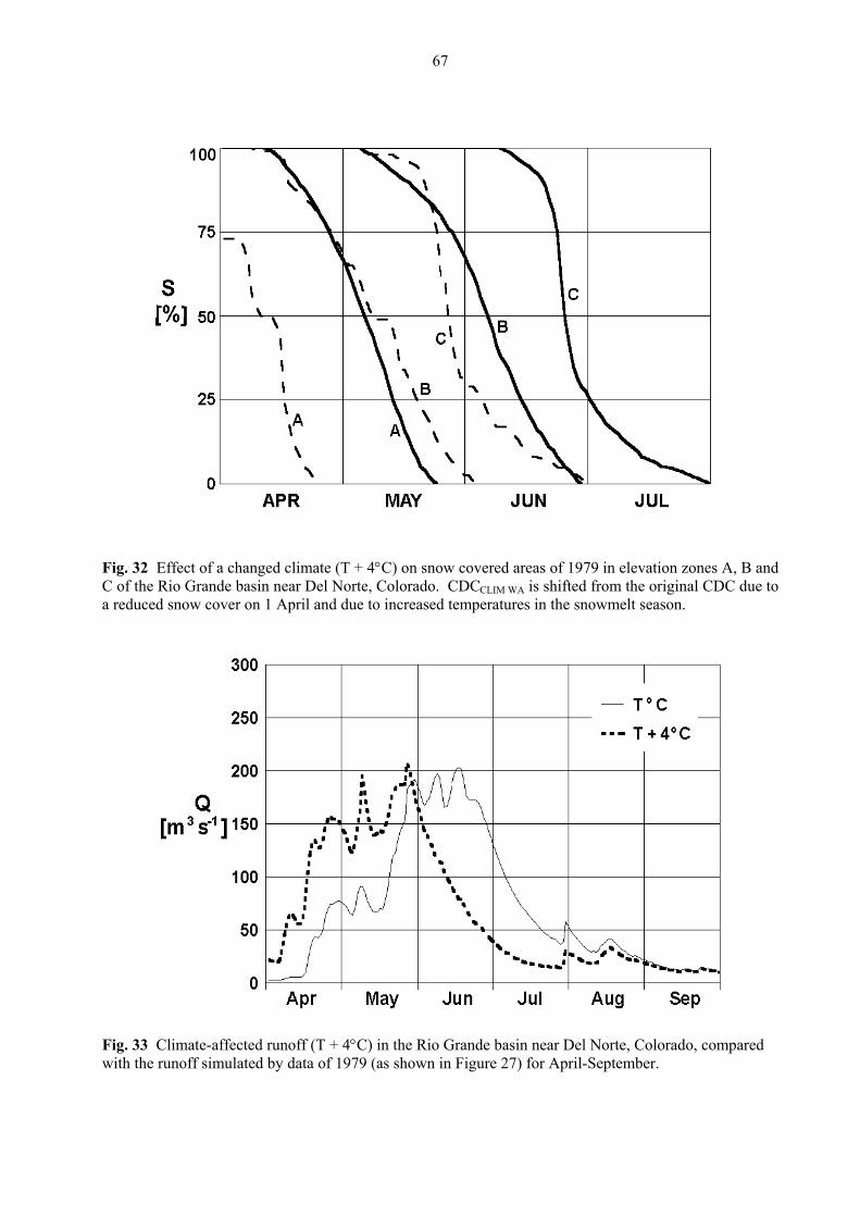
67

Fig. 32 Effect of a changed climate (T + 4°C) on snow covered areas of 1979 in elevation zones A, B and C of the Rio Grande basin near Del Norte, Colorado. CDCCLIM WA is shifted from the original CDC due to a reduced snow cover on 1 April and due to increased temperatures in the snowmelt season.

Fig. 33 Climate-affected runoff (T + 4°C) in the Rio Grande basin near Del Norte, Colorado, compared with the runoff simulated by data of 1979 (as shown in Figure 27) for April-September.

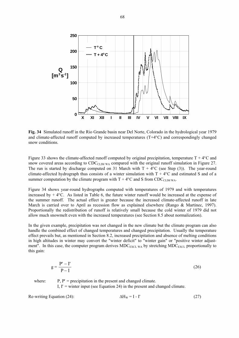
68

0

50

100

150

200

250

T C

T + 4 C

o

o

[m s ]3 -1Q

X XI XII I II III IV V VI VII VIII IX

79 nd climate-affected runoff computed by increased temperatures (T+4°C) and correspondingly changed ow conditions.

igure 33 shows the climate-affected runoff computed by original precipitation, temperature T + 4°C and ow covered areas according to CDCCLIM WA compared with the original runoff simulation in Figure 27.

The run is started by d nd limate-affected hydrograph thus consists of a winter simulation with T + 4°C and estimated S and of a mmer computation by the climate program with T + 4°C and S from CDC .

Figure 34 ydrographs computed with temperatures of 1979 and with temperatures increased by + 4°C. As listed in Table 6, the future winter runoff would be increased at the expense of the summ r runoff. The actual effect is greater because the increased climate-affected runoff in late March is arrie r t April recession flow as e lained elsewh 7). Proportionally the redistribution of runoff is relatively small because the cold winter of 1979 did not allow much snowmelt even with the increased temperatures (see Section 8.5 about normalization).

the given example, precipitation was not changed in the new climate but the climate program can also andle the combined effect of changed temperatures and changed precipitation. Usually the temperature

n 8.2, ns high altitudes in winter may convert the "winter deficit" to "winter gain" or "positive winter adjust-ent". In this case, the computer program derives MDC by stretching MDC proportionally to

Fig. 34 Simulated runoff in the Rio Grande basin near Del Norte, Colorado in the hydrological year 19asn

Fsn

ischarge computed on 31 March with T + 4°C (see Step (3)). The year-roucsu CLIM WA

shows year-round h

ec d ove o as xp ere (Rango & Martinec, 199

Inheffect prevails but, as mentioned in Sectio increased precipitation and absence of melting conditioinm EXCL WA EXCLthis gain:

g = ′ − ′P I

−P I

(26)

where: P, P′ = precipitation in the present and changed climate.

Re-writing Equation (24): (27)

I, I′ = winter input (see Equation 24) in the present and changed climate.

∆HW = I - I'

69

If there isin g = 1.2. The x-coordinates of MDCEXCL (cumulative snowmelt depth) are multiplied by g to derive MDCEXCL WA which conforms to the increased water equivalent of the snow cover on 1 April. In the summer h C results from the balance of the contradictory effects of an increased initial snow cover and of increased melting.

ge

hydrological year

no winter input in either case due to low temperatures, a precipitation increase by 20 % results

alf year, the position of CDCCLIM WA as opposed to CD

Table 6 Seasonal redistribution of runoff for 1979 in the Rio Grande near Del Norte, Colorado basin due to climate chan

winter summer 1979

106 m3 % 106 m3 % 106 m3 %

Measu 92.8 1208.96 100 red 86.53 7.2 1122.43

Computed, T 91.87 7.6 1120.15 92.4 1212.02 100

Computed, T + 4°C 146.76 12.3 1046.16 87.7 1192.92 100

8.4 Model parameters in a changed climate

SRM parameters are predetermined which requires more hydrological judgment than mechanical

anged climate. In the given example

values of both parameters were shifted accordingly by 31 days in the

September. The

calibration or optimizing. However, as has been pointed out elsewhere (Klemes, 1985, Becker & Serban, 1990, Nash & Gleick, 1991), calibration models are not suitable for climate effect studies because the parameters cannot be meaningfully adapted to the conditions of a chfrom the Rio Grande basin near Del Norte, the seasonal change of the degree-day factor a and of the runoff coefficient for snow cS was taken into account. The degree-day factor gradually increases in line with snow density while cS reflects the decline of the snow coverage and the stage of vegetation growth. Since the original CDC′s are moved by about one month earlier (see Figure 32), theclimate run. For example, a = 0.45 cm⋅°C-1⋅d-1 selected for May in the present climate was used in April in the warmer climate. The climate program provides for automatic shifting by any number of days.

hen September values are shifted to August, the value of 30 September is repeated inWshifting is stopped in January in order to prevent winter conditions being transferred to the autumn. There is no consensus yet whether a warmer climate will increase losses in which case the values of cS

and cR would be generally decreased, because a decreased evapotranspiration due to the CO2 increase might offset the temperature effect (Carlson & Bunce, 1991, Gifford, 1988). Selected parameters can be shifted or changed in accordance with the expected conditions of a future climate. Future versions will also enable the constants x, y for the recession formula to be adjusted if, for example, a steeper recession would be indicated by drier soil conditions.

70

8.5 Normalization of data to represent the present climate

The cscenaand sAppaterm aexamcase 1

1. Select a hydrological year.

thly average temperatures (see the example ahead):

∆ r – T(long term average) (∆T in each th)

3. Adjust daily temperatures of the selected year to obtain daily normalized values with daily s pre

mer half of

year 7. Simulate the runoff with Syear, Tyear, and Pyear to verify whether the estimated S and model parameters are realistic. 8. Adjust Syear to ∆T to obtain the normalized Snorm.

limate effect is evaluated by comparing present conditions with conditions modeled by a climate rio. The present conditions can be represented by precipitation, temperatures, snow covered areas imulated runoff of a single year, especially if this year appears to be a nearly average year. rently, averaging data from a number of years would be more representative. However, using long verage temperatures (which smooths out daily fluctuations) for snowmelt runoff computations, for

ple, may result in a considerable underestimation of snowmelt and runoff as mentioned in Table 5, 3. The following procedure is recommended (see also Appendix A, Example 6):

2. Determine deviations of monthly average temperature of the selected year from long term means of mon

T = Tyea different mon

fluctuation served:

Tnorm = Tyear – ∆T (∆T different in each month)

4. Determine ratios of the monthly mean precipitation of the selected year to long term monthly mean precipitation: r = (r different in each month)

P (long term average)

Pyear

5. Adjust daily precipitation of the selected year to obtain daily normalized values: Pnorm = Pyear · r (r different in each month)

he third variable, the snow cover S, is evaluated differently in the winter half and in the sumTthe year.

Winter (October – March in the Northern hemisphere) 6. Estimate S in the selected year, S , as described in Section 8.1.

71

9. Run SRM with P , T , and S to obtain the normalized winter runoff, representing the

10. Adjust Snorm to TCLIM to obtain SCLIM (see Section 8.1.). 11. Run SRM with PCLIM, TCLIM, SCLIM to obtain the climate-affected runoff.

The difference between the “Norm run” and the “Clim run” is the effect of the climate change on the winter runoff.

Summer (April – September in the Northern hemisphere)

12. Simulate runoff with Syear, Tyear, and Pyear to verify whether the model parameters are realistic (in summer Syear is obtained from satellite data). 13. Run the SRM climate program (see Section 8.4.) with Tnorm, Pnorm (in other words, consider Tnorm, Pnorm as a new climate) to derive Snorm,WA = CDCnorm,WA taking into account ∆HW obtained from winter runs. 14. Continue climate run with Pnorm, Tnorm, and Snorm to obtain the normalized summer runoff. 15. Run the SRM climate program with PCLIM, TCLIM to derive SCLIM = CDCCLIM. 16. Continue the climate run with PCLIM, TCLIM, and SCLIM to obtain the climate-affected runoff.

As mentioned for the winter half of the year, the difference between the “Norm run” and the “Clim run” in summer is the effect of the climate change on the summer runoff. In theory, identical Pnorm, Tnorm, and Snorm should be derived be derived from any selected year of present

mes. Such a result cannot be expected in view of some uncertainties involved in the procedure. ate in

ns to be available but deviates from normal onditions of the present climate.

ears with little snow are not suitable for derivation of a normalized year: if there is no snow in an elevation zone, the normalized depletion curve of the snow coverage cannot be derived. The normalized precipitation and temperatures are treated as a “changed climate”. In a climate run, a shift f parameters is sometimes advisable as mentioned in Section 8.4. It should be noted that the shift

esult, but at the same time the CDCCLIM

urves are decreased. If the users want to adjust the normalized runoff by shifting the degree-day factor, ey must cancel this automation as described in chapter 10. By taking this precaution, a parameter can be

hanged by shifting and the resulting runoff will be adjusted accordingly.

norm norm normpresent climate.

tiHowever, a normalized data set of T, P, S may be considered preferable to represent the present climcomparison with the data set from a year which happec Y

obecomes automatically part of the climate scenario. For example, if the seasonably increasing degree-dayfactors are shifted to earlier months, then higher melt rates rcthc

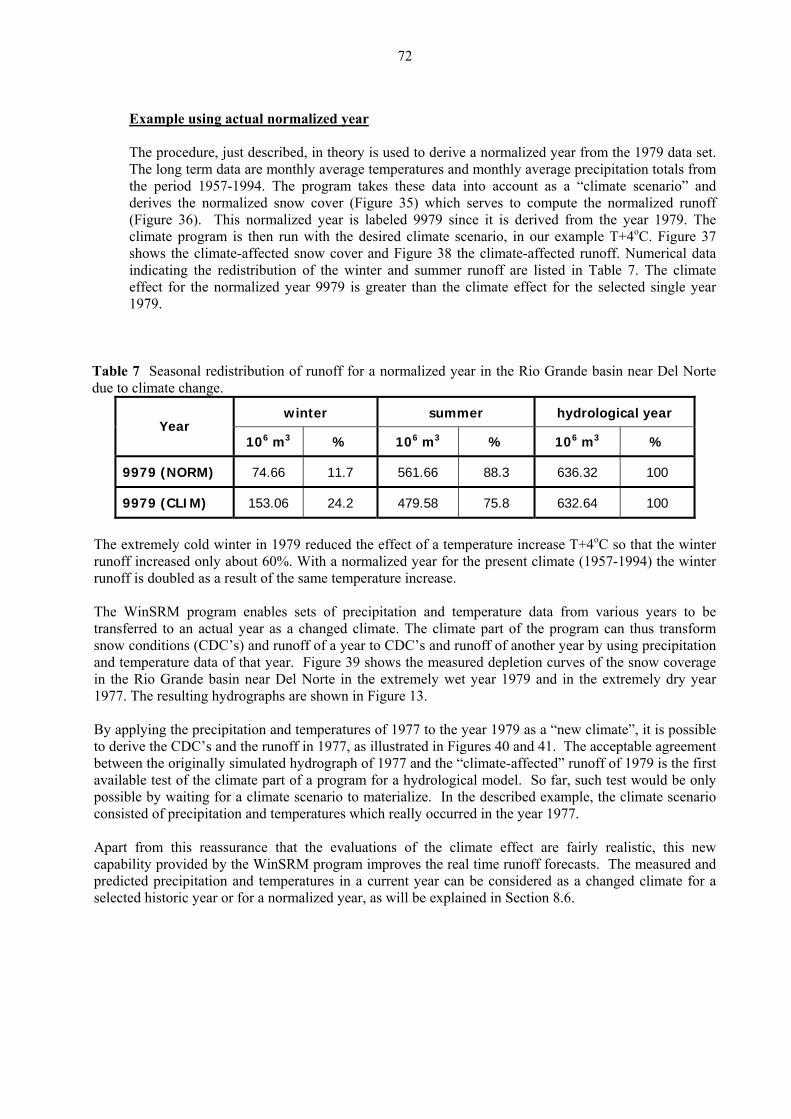
72

Example using actual normalized year The procedure, just described, in theory is used to derive a normalized year from the 1979 data set. The long term data are monthly average temperatures and monthly average precipitation totals from the period 1957-1994. The program takes these data into account as a “climate scenario” and derives the normalized snow cover (Figure 35) which serves to compute the normalized runoff (Figure 36). This normalized year is labeled 9979 since it is derived from the year 1979. The climate program is then run with the desired climate scenario, in our example T+4oC. Figure 37 shows the climate-affected snow cover and Figure 38 the climate-affected runoff. Numerical data indicating the redistribution of the winter and summer runoff are listed in Table 7. The climate effect for the normalized year 9979 is greater than the climate effect for the selected single year 1979.

Table 7 Seasonal redistribution of runoff for a normalized year in the Rio Grande basin near Del Norte due to climate change.

winter summer hydrological year Year

106 m3 % 106 m3 % 106 m3 %

9979 (NORM) 74.66 11.7 561.66 88.3 636.32 100

9979 (CLIM) 153.06 24.2 479.58 75.8 632.64 100

The extremely cold winter in 1979 reduced the effect of a temperature increase T+4oC so that the winter runoff increased only about 60%. With a normalized year for the present climate (1957-1994) the winter runoff is doubled as a result of the same temperature increase. The WinSRM program enables sets of precipitation and temperature data from various years to be transferred to an actual year as a changed climate. The climate part of the program can thus transform snow conditions (CDC’s) and runoff of a year to CDC’s and runoff of another year by using precipitation and temperature data of that year. Figure 39 shows the measured depletion curves of the snow coverage in the Rio Grande basin near Del Norte in the extremely wet year 1979 and in the extremely dry year 1977. The resulting hydrographs are shown in Figure 13. By applying the precipitation and temperatures of 1977 to the year 1979 as a “new climate”, it is possible to derive the CDC’s and the runoff in 1977, as illustrated in Figures 40 and 41. The acceptable agreement between the originally simulated hydrograph of 1977 and the “climate-affected” runoff of 1979 is the first available test of the climate part of a program for a hydrological model. So far, such test would be only possible by waiting for a climate scenario to materialize. In the described example, the climate scenario consisted of precipitation and temperatures which really occurred in the year 1977. Apart from this reassurance that the evaluations of the climate effect are fairly realistic, this new capability provided by the WinSRM program improves the real time runoff forecasts. The measured and predicted precipitation and temperatures in a current year can be considered as a changed climate for a selected historic year or for a normalized year, as will be explained in Section 8.6.

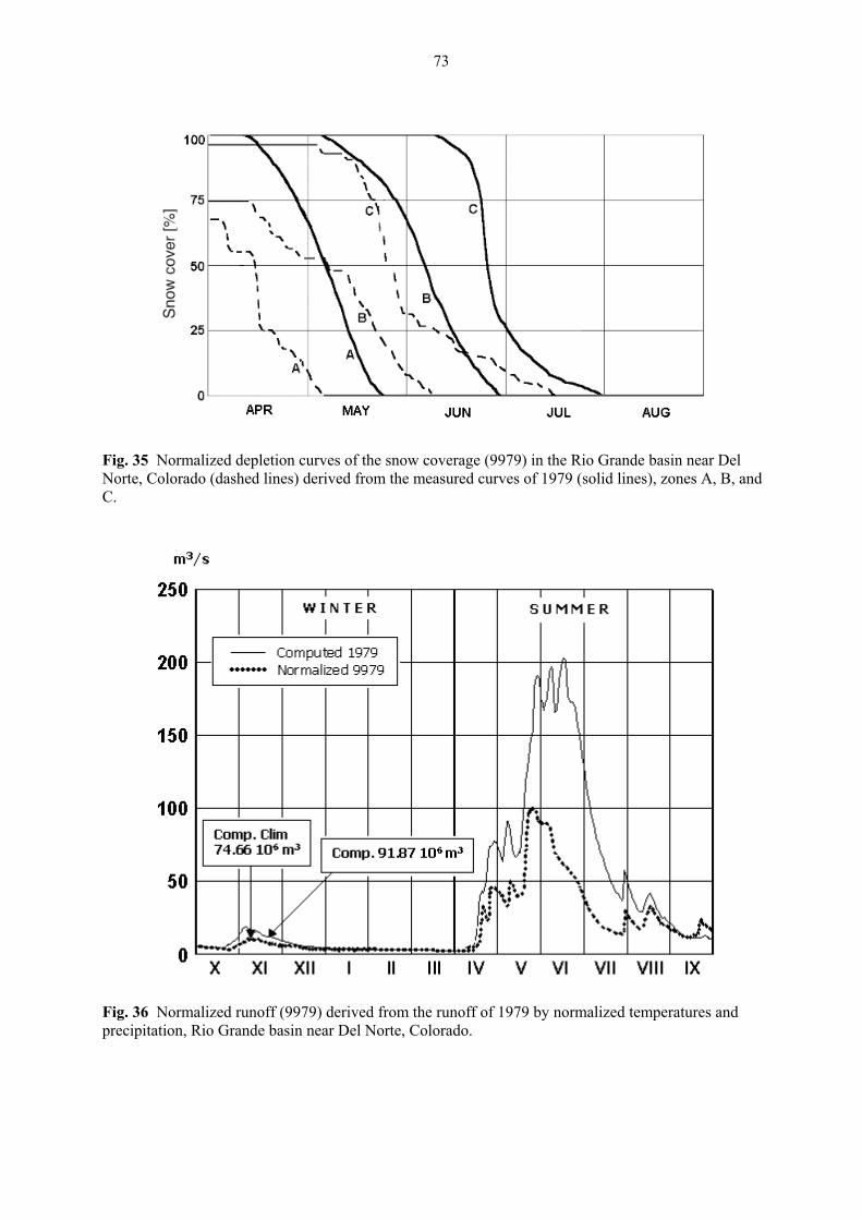
73

Fig. 35 Normalized depletion curves of the snow coverage (9979) in the Rio Grande basin near Del Norte, Colorado (dashed lines) derived from the measured curves of 1979 (solid lines), zones A, B, and C.

Fig. 36 Normalized runoff (9979) derived from the runoff of 1979 by normalized temperatures and precipitation, Rio Grande basin near Del Norte, Colorado.

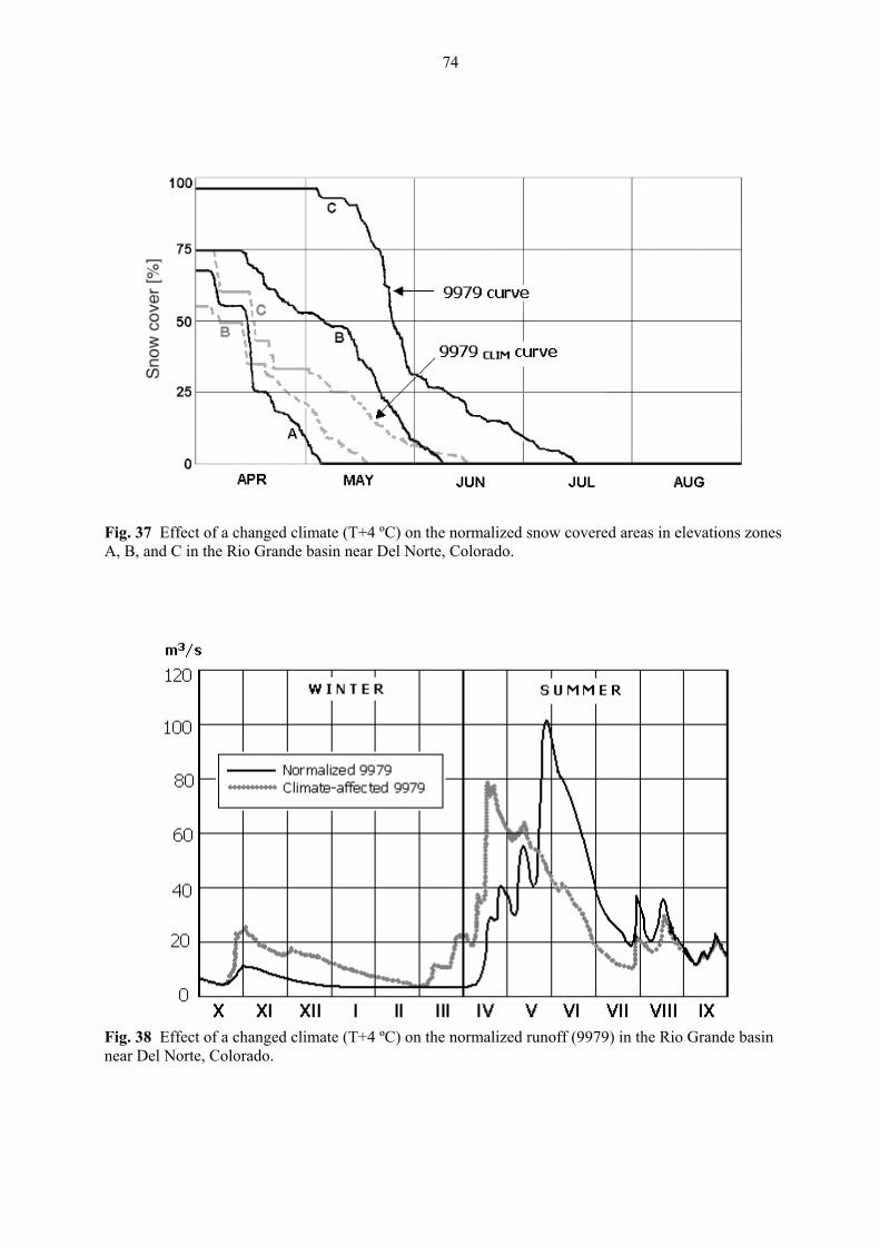
74

ged climate (T+4 ºC) on the normalized snow covered areas in elevations zones Fig. 37 Effect of a chanA, B, and C in the Rio Grande basin near Del Norte, Colorado.

Fig. 38 Effect of a changed climate (T+4 ºC) on the normalized runoff (9979) in the Rio Grande basin near Del Norte, Colorado.

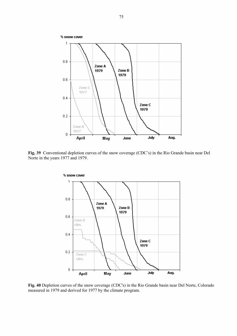
75

Fig. 39 Conventional depletion curves of the snow coverage (CDC’s) in the Rio Grande basin near Del Norte in the years 1977 and 1979.

Fig. 40 Depletion curves of the snow coverage (CDC's) in the Rio Grande basin near Del Norte, Colorado measured in 1979 and derived for 1977 by the climate program.

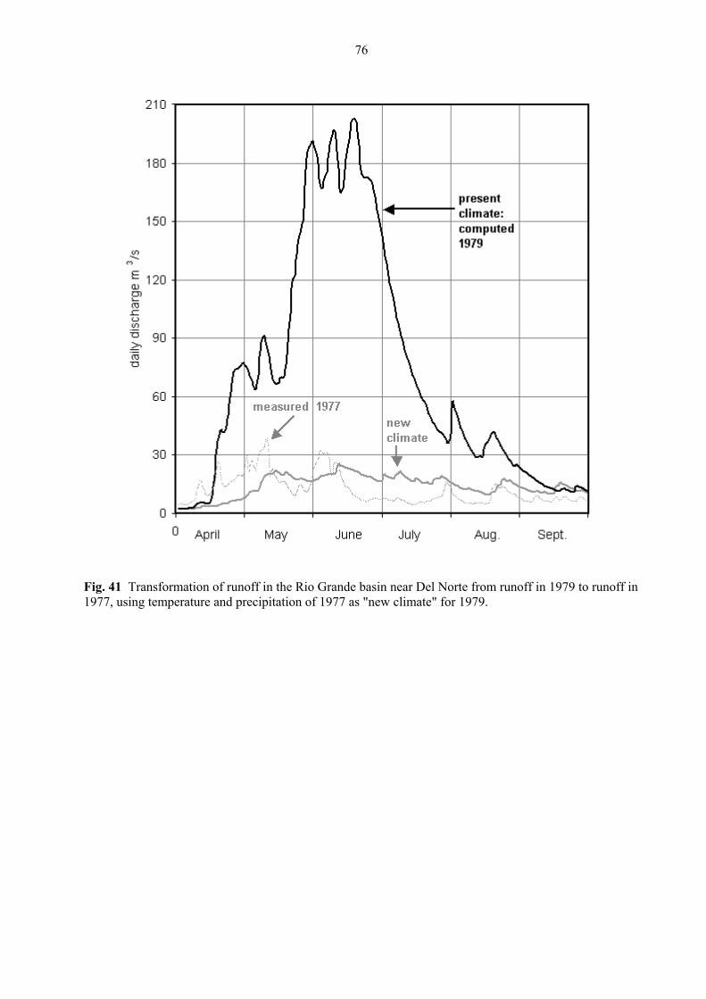
76

Fig. 41 Transform runoff in 1979 to runoff in

1979. ation of runoff in the Rio Grande basin near Del Norte from

perature and precipitation of 1977 as "new climate" for 1977, using tem

77

.6 WinSRM to improve real time runoff forecasts

With WinSRM it is no longer necessary to assemble a set of modified depletion curves, MDC’s, as shown in Figure 21 in order to forecast the future course of the conventional depletion curves, CDC’s. In a new basin, where these graphs are not yet available, it is sufficient to have one historical year with good satellite data on snow covered areas and the usual daily values of temperature and precipitation. Based on this data set, runoff starting on 1 April can be forecasted as follows:

1. Runoff is simulated for the available historical year in order to verify the preselected model parameters.

2. The climate program is run for the winter half of the year with the known values

of precipitation and temperature, T and P, of the forecast year (F).

3. Snow water equivalent (HW) on 1 April of the historical year (A) is evaluated using the modified depletion curves MDCEXCL A

4. Snow water equivalent on 1 April of the forecast year is evaluated from the

winter deficit or excess as shown in Equation (24), and the curve MDCEXCL F is derived accordingly.

The runoff in the summer half of the year is composed of a guaranteed runoff volume from MDCEXCL F (taking into account the losses) and of the forthcoming precipitation. Seasonal runoff forecasts can be issued for different precipitation eventualities.

5. The climate program is run for the summer half of the year considering dailnormalized T, P (see Section 8.5) as a “new climate” and MDCCLIM WA (in other

6. The conventional curve CDC F is derived from MDCINCL F.

7. SRM is run with Tnorm , Pnorm , and CDC F . This is a day-to-day forecast for the next 6 months, assuming normal precipitation and temperature. This forecast can be updated by actual and forecasted temperatures and precipitation. It is also possible to use as a new climate, instead of Tnorm ,and Pnorm , the T and P values of an extremely dry or extremely wet summer, which could occur with a certain probability.

8

y

words MDCINCL F ) is derived.

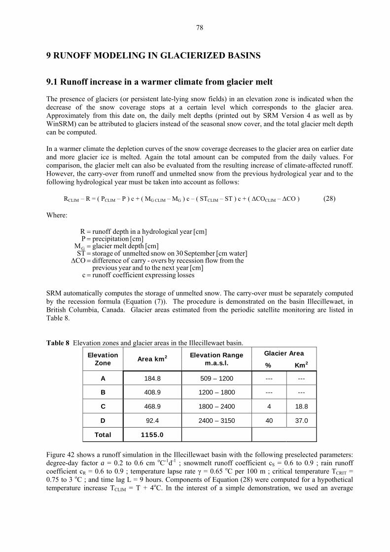
78

9 RUNOFF MODELING IN GLACIER ZED BASINS

crease in a warmer climate from glacier melt

he presence of glaciers (or persistent late-lying snow fields) in an elevation zone is indicated when the hich corresponds to the glacier area.

pproximately from this date on, the daily melt depths (printed out by SRM Version 4 as well as by inSRM) can be attributed to glaciers instead of the seasonal snow cover, and the total glacier melt depth

can be computed.

In a warmer climate the deplet he glacier area on earlier date nd more glacier ice is melted. Again the total amount can be computed from the daily values. For

the carry-over from runoff and unmelted snow from the previous hydrological year and to the llowing hydrological year must be taken into account as follows:

) c + G ) c – ( STCLIM – ST (28)

anear evious fromflow recessioncar

w[cmSeptember 30nme[cm] depthmelt glacier M

[cm] ionprecipitat P[cm] year alhydrologica in depth runoff R

G

=

===

M automatically com utes th storag of unm lted snow. The carry-o computed ula (Equation (7)). The onstrated on the basin Illecillewaet, in

ritish Columb lacier areas estimated from the periodic satellite monitoring are listed in able 8.

able 8 Elevation zones and glacier areas in the Illecillewaet basin.

I

9.1 Runoff in

Tdecrease of the snow coverage stops at a certain level wAW

ion curves of the snow coverage decreases to t

acomparison, the glacier melt can also be evaluated from the resulting increase of climate-affected runoff. However, fo

RCLIM – R = ( PCLIM – P ( MG CLIM – M ) c + ( ∆COCLIM – ∆CO ) Where:

losses expressingt coefficien runoff c[cm]next year the tod ypr

theby overs-ryof difference COater] onsnow u lted of storage ST

=∆=

SR p e e e ver must be separately

y the recession form procedure is dembB ia, Canada. GT T

Glacier Area Elevation Zone Area km2 Elevation Range

m.a.s.l. % Km2

A 184.8 509 – 1200 --- ---

B 408.9 1200 – 1800 --- ---

C 468.9 1800 – 2400 4 18.8

D 92.4 2400 – 3150 40 37.0

Total 1155.0

Figure 42 shows a runoff simulation in the Illecillewaet basin with the following preselected parameters: egree-day factor a = 0.2 to 0.6 cm oC-1d-1 ; snowmelt runoff coefficient c = 0.6 to 0.9 ; rain runoff d S

coefficient cR = 0.6 to 0.9 ; temperature lapse rate γ = 0.65 oC per 100 m ; critical temperature TCRIT = 0.75 to 3 oC ; and time lag L = 9 hours. Components of Equation (28) were computed for a hypothetical temperature increase TCLIM = T + 4oC. In the interest of a simple demonstration, we used an average

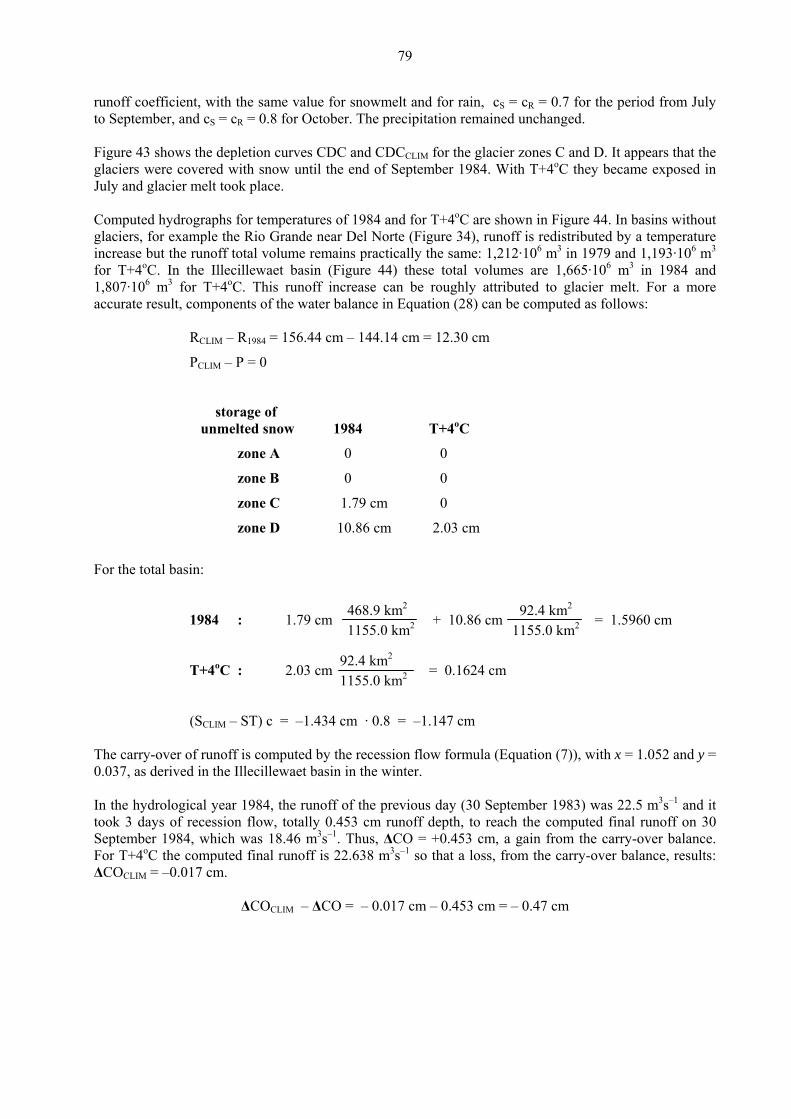
79

runoff coefficient, with the same value for snowmelt and for rain, cS = cR = 0.7 for the period from July to September, and cS = cR = 0.8 for October. The precipitation remained unchanged.

T+4 C they became exposed in ly and glacier melt took place.

cm – 144.14 cm = 12.30 cm

For the total basin:

1984 : 1.79 cm + 10.86 cm = 1.5960 cm T+4oC : 2.03 cm

(SCLIM – ST) c = –1.434 The carry-over of runoff is computed by t0.037, as derived in the Illecillewaet basin In the hydrological year 1984, the runoff took 3 days of recession flow, totally 0.4September 1984, which was 18.46 m3s–1.For T+4oC the computed final runoff is 2∆COCLIM = –0.017 cm.

∆COCLIM – ∆CO

Figure 43 shows the depletion curves CDC and CDCCLIM for the glacier zones C and D. It appears that the glaciers were covered with snow until the end of September 1984. With o

Ju Computed hydrographs for temperatures of 1984 and for T+4oC are shown in Figure 44. In basins without glaciers, for example the Rio Grande near Del Norte (Figure 34), runoff is redistributed by a temperature increase but the runoff total volume remains practically the same: 1,212·106 m3 in 1979 and 1,193·106 m3 for T+4oC. In the Illecillewaet basin (Figure 44) these total volumes are 1,665·106 m3 in 1984 and 1,807·106 m3 for T+4oC. This runoff increase can be roughly attributed to glacier melt. For a more accurate result, components of the water balance in Equation (28) can be computed as follows:

RCLIM – R1984 = 156.44

PCLIM – P = 0

storage of unmelted snow 1984 T+4oC

zone A 0 0

zone B 0 0

zone C 1.79 cm 0

zone D 10.86 cm 2.03 cm

2 2

468.9 km2

1155.0 k

m

= 0.1624 cm

cm · 0.8 = –1.147 cm

he recession flow formula (E in the winter.

of the previous day (30 Sep53 cm runoff depth, to rea Thus, ∆CO = +0.453 cm, 2.638 m3s–1 so that a loss, f

= – 0.017 cm – 0.453 cm =

2

92.4 km2

1155.0 km
92.4 km2
1155.0 km

quation (7)), with x = 1.052 and y =

tember 1983) was 22.5 m3s–1 and it ch the computed final runoff on 30 a gain from the carry-over balance. rom the carry-over balance, results:

– 0.47 cm

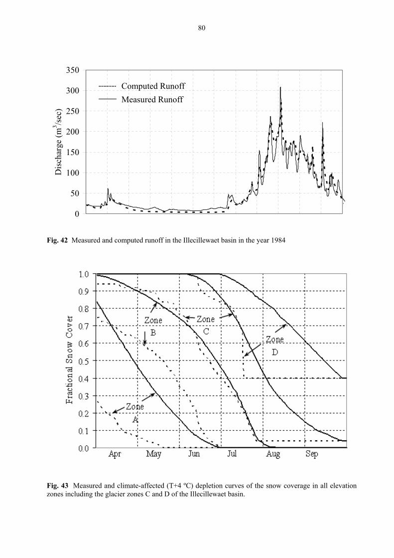
80

350

Computed RunoffMeasured Runoff

300

100

150

200

250

Dis

char

ge (m

3 /sec

)

50

0

Fig. 42 Measured and computed runoff in the Illecillewaet basin in the year 1984

Fig. 43 Measured and climate-affected (T+4 ºC) depletion curves of the snow coverage in all elevation zones including the glacier zones C and D of the Illecillewaet basin.

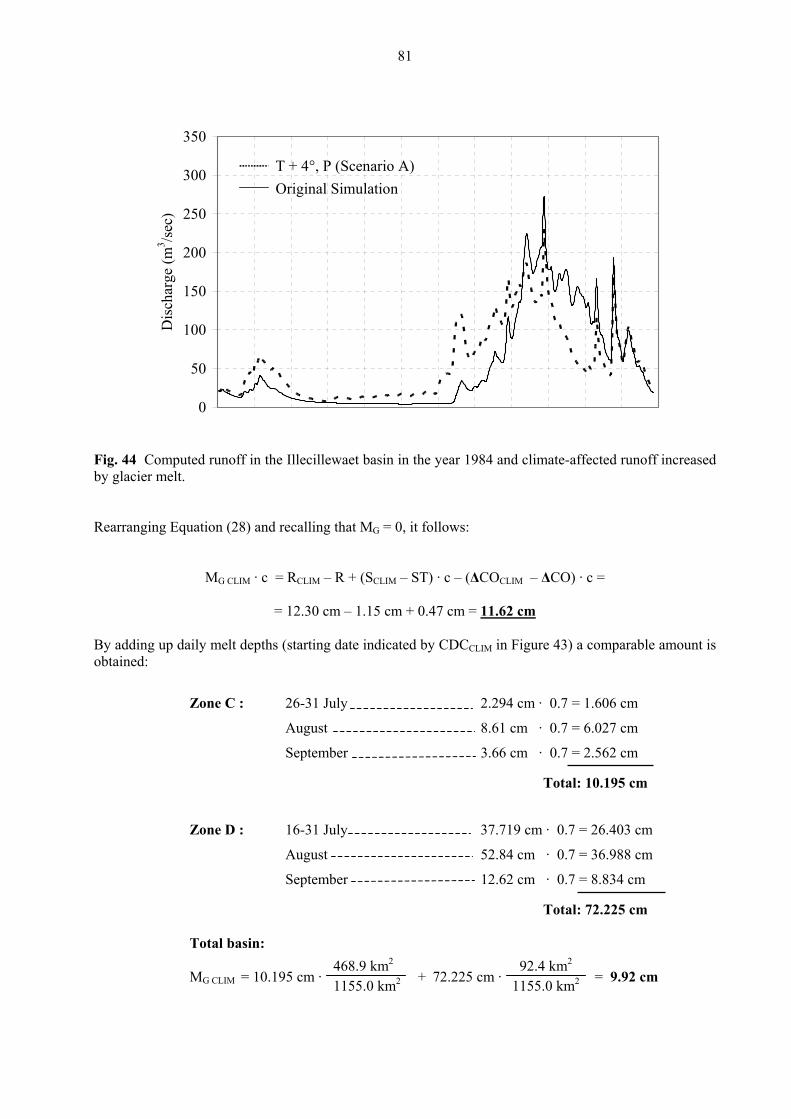
81

300

350

T + 4°, P (Scenario A)Original Simulation

0

50

100

150

Dis

char

ge (m

200

3

250

/sec

)

Fig. 44 Computed runoff in the Illecillewaet basin in the year 1984 and climate-affected runoff increased

y glacier melt. b Rearranging Equation (28) and recalling that MG = 0, it follows:

MG CLIM · c = RCLIM – R + (SCLIM – ST) · c – (∆COCLIM – ∆CO) · c =

= 12.30 cm – 1.15 cm + 0.47 cm = 11.62 cm By adding up daily melt depths (starting date indicated by CDC in Figure 43) a comparable amount is obtained:

CLIM

Zone C : 26-31 July 2.294 cm · 0.7 = 1.606 cm

August 8.61 cm · 0.7 = 6.027 cm

September 3.66 cm · 0.7 = 2.562 cm

Zone D : 16-31 July 37.719 cm · 0.7 = 26.403 cm

August 52.84 cm · 0.7 = 36.988 cm

September 12.62 cm · 0.7 = 8.834 cm

Total: 72.225 cm

Total basin: MG CLIM = 10.195 cm 72.225 cm · 9.92 cm

Total: 10.195 cm

· + = 2
468.9 km2
1155.0 km2

92.4 km2

1155.0 km

82

In terms of volume, the net glacier contribution to runoff is 134.2 ·106 m3 according to the balance

ample assumes that the warm year occurs in present times. In reality, it can be expected ed, the glacier areas will be in the meantime reduced. d thus be needed, as outlined in the next section.

9.2 Long term behavior of glaciers in a warming climate

The WinSR to use as a “new climate”, a set of normalized daily mperatures and precipitation to derive a normalized year (Section 8.5), as well as a data set (T,P) of a

historical year, if available, and a data set of a future year, if the data can be generated.

ate scenarios into account in one step. For example, the present d by conditions predicted for the year 2050. This procedure is inadequate

perature will not continuously increase by a fraction of a degree each year. On

stochastic series of temperature and precipitation data can be generated (Gyalistras et al, 1994) which can reach the values given by a climate scenario in the year in question. In the starting year, the depletion curves of the snow coverage and the glacier area must be known apart from temperature and precipitation data. The glacier melt volume and the carry-over of the unmelted snow (if any) to the next year are computed. From the glacier melt volume, the reduced glacier area for the next year is estimated by statistically derived relations between the volume and area of glaciers (Bahr et al, 1997). With this new area together with temperature and precipitation data, we can evaluate next year’s CDC’s, the glacier melt volume and carry-over of unmelted snow to the next year. These computations are repeated year by year until the year for which the climate scenario is predicted. In a cold year, the carry-over of unmelted snow will increase and the CDC’s will probably not decline to the glacier area, signaling no glacier melt. Should the stochastic series indicate a sequence of cold years, the amount of unmelted snow by the end of each hydrological year will be built up. It cannot be determined which part of this snow will become part of a glacier. However, sooner or later this snow will be melted, the CDC’s will decrease to the last derived glacier area and the glacier melt will start again. Each year the glacier melt volume will result in a reduced glacier area for the next year, until the ultimate disappearance of glaciers. Whether this will appen before or after the target year depends on the intervening weather conditions.

spite of inherent approximations, this method may prove to be more realistic than mere speculations bout the fate of glaciers. As a practical exploit for the management of water resources, in particular

hydropower generation, the increase of runoff from glacierized basins in the coming decades can be evalua

method, 114.6 ·106 m3 from computed daily melt depths, and 142 ·106 m3 according to the increase of the yearly runoff. This last amount is of course obtained only from an incomplete water balance. This ypothetical exh

that when such temperature increase is reachModeling of a long term sequence of years woul

M program enables climate runste

So far, hydrological models took climclimatic conditions were replacefor glaciers because temthe contrary, as in the past, temperature will fluctuate from year to year with an underlying increasing trend. A

h Ina

ted.

83

10 SR DOWS (WI

0.1 Program overview

a complete modeling environment in which snowmelt runoff is mulated for mountain basins where snowmelt provides a major contribution to that runoff. The model

manages a database of physical data for a given basin, and any number of individual simulation data sets, stored as unique tables in the database. Each simulation is an independent entity operating on a 2-366 day subset of the database’s physical database. Simulation results are available to the user via a series of tabular reports and an extensive library of graphical plots. The model environment includes a unique ability to design complex ‘scenarios’ that describe a future changed climate in a basin, and then simulate the effect of such a scenario on runoff for that basin.

10.1.1 Historical background

The Martinec/Rango Snowmelt Runoff Model (SRM) was originally a FORTRAN model designed to operate on an IBM 370-series mainframe computer. The first computerized version of the model was developed by Martinec et al. (1983). In 1986 the model's FORTRAN code was downloaded to an IBM PC and modified to operate in the PC environment. That same year a decision was made to develop a unique PC-oriented version of the model, taking full advantage of the PC's inherent capabilities. The result of that decision was Micro-SRM, Version 1.0. Additional refinements were incorporated in several subsequent Micro-SRM Versions up to and including 4.0. However, SRM itself remained unchanged and relatively simple, so that the computations by Equation (1) could still be performed by any pocket calculator which has a function xy. The DOS PC program automatically handles the multiple input of temperature and precipitation for up to 8 elevations zones of a basin, any desired lag time, and complicated snow/rain situations. A model simulation for up to 365 days is finished within several seconds, the computed hydrograph is immediately displayed in

printed. Also, the achieved accuracy is utomatically computed and displayed. A summary parameter values can be displayed after each run

so that adjustments can be made and their effect assessed. SRM does not require numerous runs because calibration is not necessary. The ease with which the results are obtai not lead to ent of the deterministic approach of SRM by a "try and see" philosophy. SRM is designed to operate with physically based estimates of parameters that should not require much er the initi equently improved not b the param ing errors in data sets and in the input of variables. A prime consideration in the design o lop a snowmelt modeling "environment" such that the model user was provided not just model algorithms, but a complete set of tools for managing the associated model processes: da , and results. Traditionally, th min based model has been the accum of l drive the simulation, with actual execution n. Recognizing this, we hose to pattern the design of Micro-SRM after that originally developed during the automation of the oil Conservation Service's (SCS) Technical Release Number 55 (TR-55), Urban Hydrology for Small atersheds (Soil Conservation Service, 1986). This joint ARS/SCS effort provided valuable experience developing highly interactive "front-ends" for interfacing complex models with model users.

M FOR WIN NSRM) COMPUTER PROGRAM

1

WinSRM provides the user with si

comparison with the measured discharge and, if desired, quicklya of

ned should a replacem

change afty adjusting

al selection. Seemingly unsatisfactory results have been freters but by correct

f Micro-SRM was to deve

ta entry, storage and retrieval, display of datag and error prone activity involved in using any physically

arge amounts of input data in the form and format needed toof the model a trivial task by compariso

e most time consuulation

cSWin

84

The approach used by the ARS/SCS programmfficient, easy to use, highly interactive data

ing team that automated TR-55 was to develop an entry/manipulation environment, and include model

0.1.2 Program description

ws (WinSRM) is the first version of SRM that has been adapted stem (Win 95/98/2000/XP). Limitations imposed on

e research by the physical constraints of DOS operating system, as well as its relative ary reasons for the transition to Windows.

g identical simulation results to those obtained by the DOS ersion of the model. The graphical user interface (GUI) and data storage philosophy have undergone a

complete redesign to take advantage of the enhanced capabilities available on the modern “windows” latform. All of the original DOS output products (graphs and reports) remain available, with

enhancements provided that im ine quality.

Basins may now consist of up to 16 elevation zones. Modern database technology is utilized to manage quirements of the model. Storage is organized using the concept of a ‘basin’ database.

ithin a basin database resides a single copy of the physical variables for the basin’s ‘period of record’. ulations ted in the same database along with

supporting inform io e scenario definitions.

The most significant im ulation. The limitations impo ing a much more detailed and robust definition of change to be studied.

Finally, the path of future research using the model has been laid by moving to an operating system and a model design that minimizes or removes the restraints to development inherent in the earlier design and operating system environment.

The current version of the model, WinSRM, Version 1.11, was developed using Microsoft Visual Basic 6.0 and contains one custom control, Spread 2.5, from Farpoint Technologies1.

ealgorithms as just one of many functions that support and use that environment (Cronshey et al., 1985). Micro-SRM consists of an integration of the mainframe SRM FORTRAN algorithms converted to Basic and a variation of TR-55's data entry/data management algorithms.

1

The Snowmelt-Runoff Model for Windofor use with the Microsoft Windows operating syexisting and futurobsolescence, were the prim

This new version of the program is compatible with pre-existing DOS .SRM data files. The basic SRM model algorithm remains unchanged, producinv

pprove on-line analysis and usability, and off-l

the data storage reWAll the sim developed for the basin are likewise loca

n used by the modeler, such as climate changat

provement in the model’s capability is in the area of climate change simsed on climate change processing by DOS have been removed, allow

1 Trademarks used in this document (e.g., IBM PC, IBM CORP., Visual BASIC, Microsoft Corp.; Spread grid OCX, Farpoint Technologies) are used solely for the purpose of providing specific information. Mention of a trade name does not constitute a guarantee or warranty for the product by the U.S. Department of Agriculture or an endorsement by the Department over other products not mentioned.

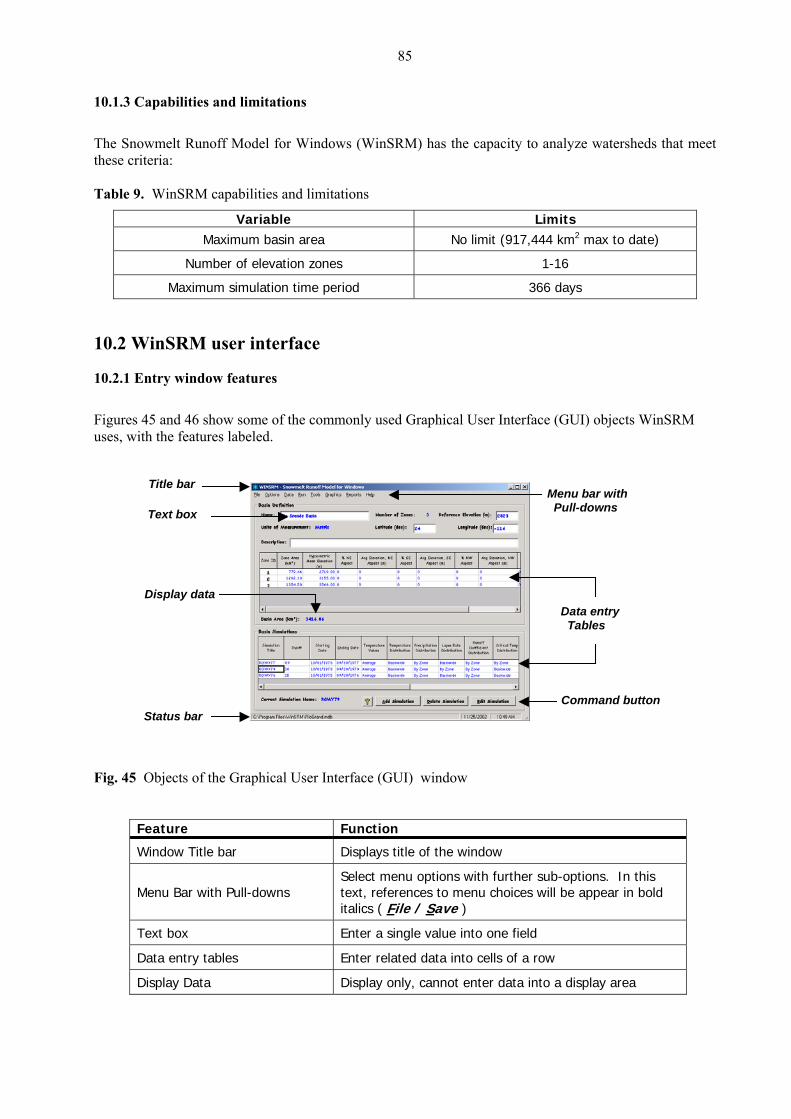
85

10.1.3 Capabilities and limitations

Windows (WinSRM) has the capacity to analyze watersheds that meet ese criteria:

capabilities and limitations

The Snowmelt Runoff Model for th Table 9. WinSRM

Variable Limits Maximum basin area No limit (917,444 km2 max to date)

Number of elevation zones 1-16

Maximum simulation time period 366 days

10.2 WinSRM user interface

10.2.1 Entry window features

Figures 45 and 46 show some of the commonly used Graphical User Interface (GUI) objects WinSRM uses, with the features labeled.

Title bar

Text box

Menu bar with Pull-downs

Display dataData entry Tables

Status barCommand button

Fig. 45 Objects of the Graphical User Interface (GUI) window

Feature Function

Window Title bar Displays title of the window

Menu Bar with Pull-downs Select menu options with further sub-options. In this text, references to menu choices will be appear in bold italics ( File / Save )

Text box Enter a single value into one field

Data entry tables Enter related data into cells of a row

Display Data Display only, cannot enter data into a display area

86

Command button Click to access the functionality. In this text, references to command buttons will appear in a shaded, bounded box ( Help ).

Status Bar Displays program status information

Check Box – any combination oactive choices may be checked.

f

In tive choices a ‘grayed-out’.ac

Option button – used whenonly onchoices

e of two or more is appropriate.

Command button

Fig. 46 Additional d b

Feature Function

GUI objects use y the WinSRM interface

Check box Used to display multiple choices from which the user can select one or more.

Option button Used to display multiple choices from which only one choice may be selected.

Command button

Begin, interrupt, or end a process. When chosen, a command button appears ‘pressed-in’. Access the button

corresponding hot (undefunctions using the keyboard by pressing the ‘Alt’ key, then the rlined) key.

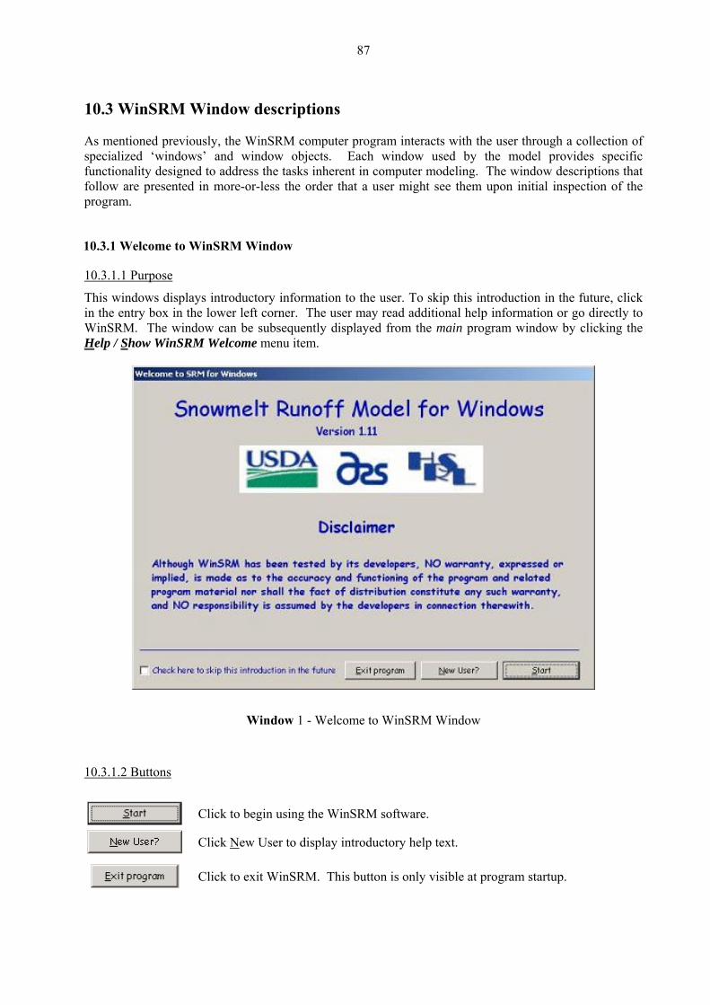
87

10.3 WinSR n As mentioned previously, the WinSRM compu llection of spec in s specific functionality des h that follow are prese pection of the program.

0.3.1 Welcome to WinSRM Window

.1 Purpose

M Window descriptio s

ter program interacts with the user through a co Each window used by the model provideerent in computer modeling. The window descriptionsr that a user might see them upon initial ins

ialized ‘w

dows’ and window objects.igned to address the tasks innted in more-or-less the orde

1

10.3.1

his windows displays introductory information to the user. To skip this introduction in the future, click Tin the entry box in the lower left corner. The user may read additional help information or go directly to WinSRM. The window can be subsequently displayed from the main program window by clicking the Help / Show WinSRM Welcome menu item.

Window 1

10.3.1.2 Buttons

- Welcome to WinSRM Window

Click to begin using the WinSRM software.

Click New User to display introductory help text.

Click to exit WinSRM. This button is only visible at program startup.

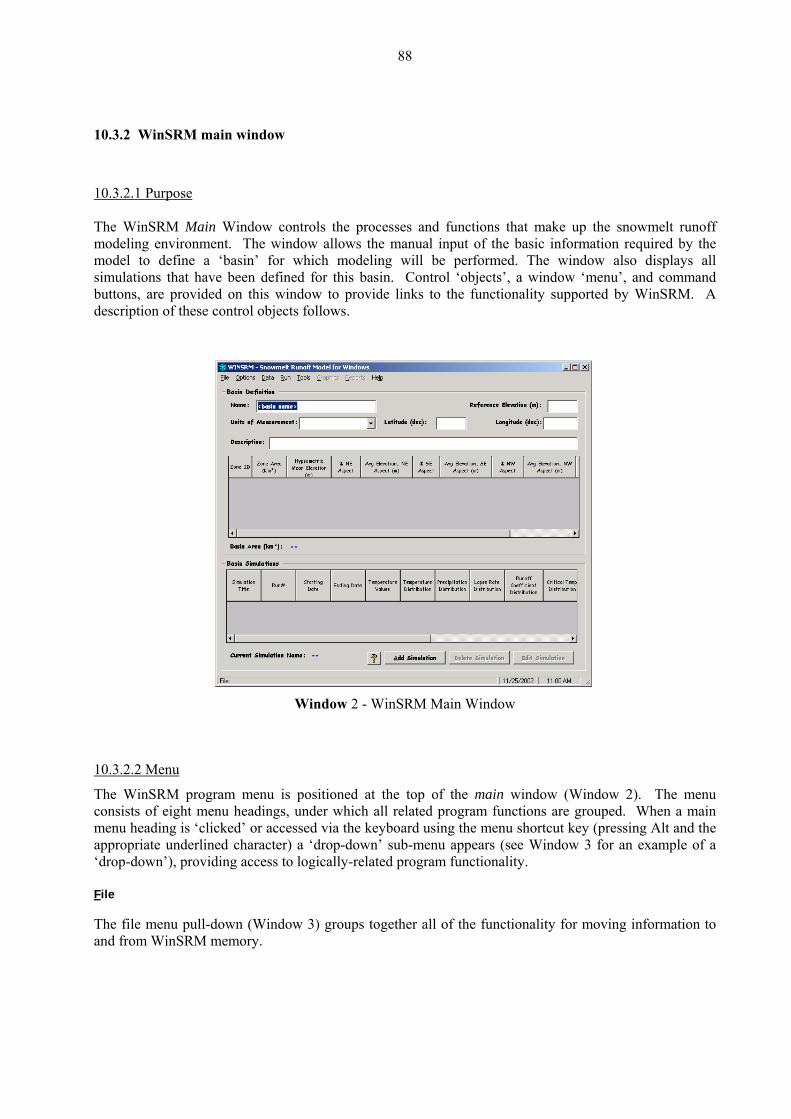
88

10.3.2 WinSRM main window

10.3.2.1 Purpose The WinSRM Main Window controls the processes and functions that make up the snowmelt runoff

odeling environment. The window allows the m l input of the basic information required by the odel to define a ‘basin’ for which modeling will be performed. The window also displays all mulations that have been defined for this basin. Control ‘objects’, a window ‘menu’, and command uttons, are provided on this window to provide links to the functionality supported by WinSRM. A escrip these ts follows.

m anuamsibd tion of control objec

Window 2 - WinSRM Main Window

0.3.2.2 Menu1

The WinSRM program menu is positioned at the top of the main window (Window 2). The menu consists of eight menu headings, under which all related program functions are grouped. When a main menu heading is ‘clicked’ or accessed via the keyboard using the menu shortcut key (pressing Alt and the appropriate underlined character) a ‘drop-down’ sub-menu appears (see Window 3 for an example of a ‘drop-down’), providing access to logically-related program functionality. File The file menu pull-down (Window 3) groups together oving information to and from WinSRM memory.

all of the functionality for m

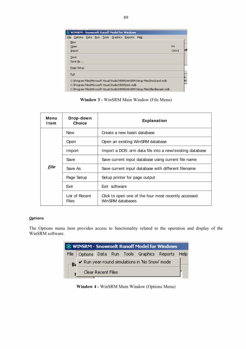
89

Window 3 - WinSRM Main Window (File Menu)

Menu Item

Drop-down Choice Explanation

New Create a new basin database

Open Open an existing WinSRM database

Import Import a DOS .srm data file into a new/existing database

Save Save current input database using current file name

Save As Save current with different filename input database

Page Setup Setup printer for page output

Exit Exit software

File

List of Recent Files

Click to open one of the four most recently accessed WinSRM databases

Options The Options menu item provides access to functionality related to the operation and display of the WinSRM software.

Window 4 - WinSRM Main Window (Options Menu)

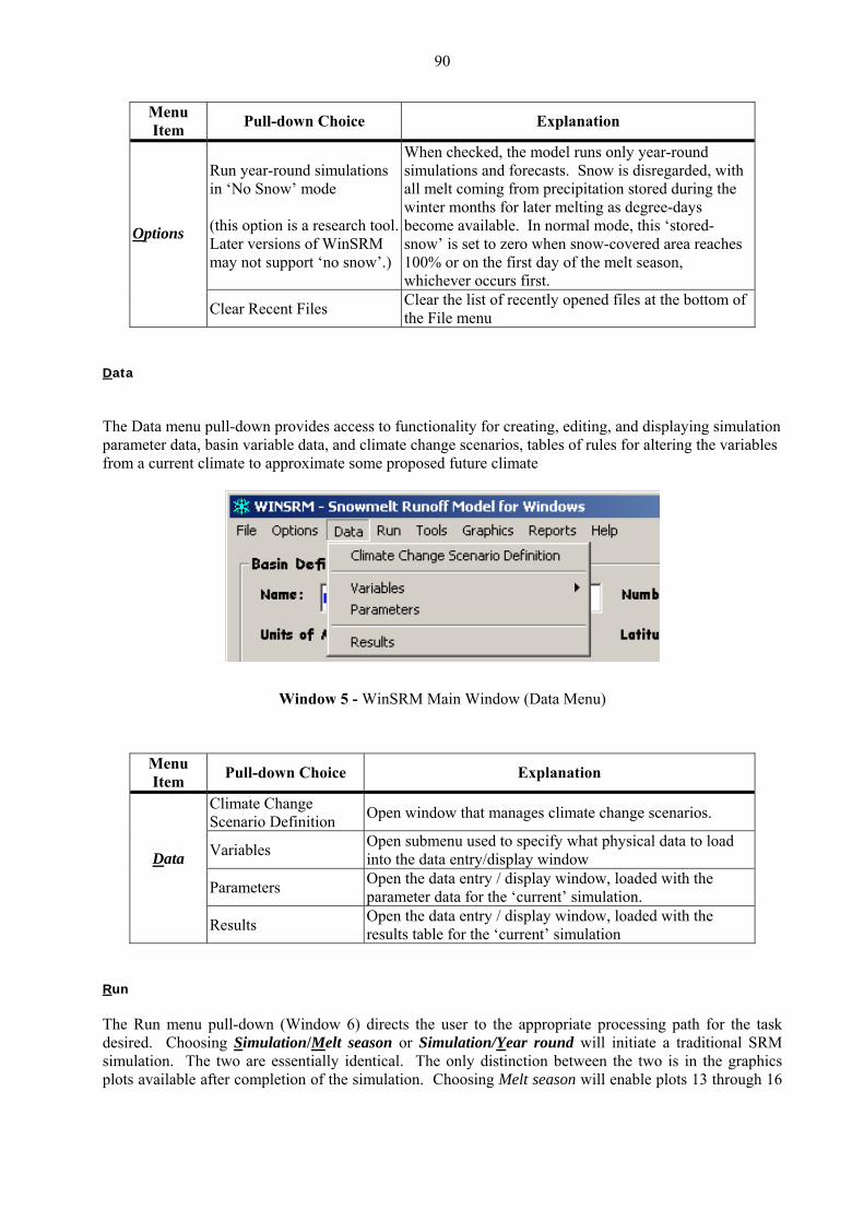
90

Menu Item Pull-down Choice Explanation

Run year-round simulations in ‘No Snow’ mode (this option is a research tool. Later versions of WinSRM may not s

When checked, the model runs only year-round simulations and forecasts. Snow is disregarded, with all melt coming from precipitation stored during the winter months for later melting as degree-days become available. In normal mode, this ‘stored-snow’ s set to zero when snow-covered area re ches

elt season, upport ‘no snow’.) 100% or on the first day of the mwhichever occurs first.

i aOptions

Clear Recent Files Clear the list of recently opened files at the bottom of the File menu

Data The Data menu s acce nd displaying simulation parame , le data, and climfrom a current c te so

pull-down providebasin variab

ss to functionality for creating, editing, aate change scenarios, tables of rules for altering the variables ter data

limate to approxima me proposed future climate

Window 5 - WinSRM Main Window (Data Menu)


Climate Change Scenario Definition Open window that manages climate change scenarios.

Va abl Open submenu used to specify what physical data to load

ri es into the data entry/display window

Parameters Open the data entry / display window, loaded with the parameter data for the ‘current’ simulation.

Data

Results Open the data entry / display window, loaded with the results table for the ‘current’ simulation

Run The Run menu pull-down (Window 6) directs the user to the appropriate processing path for the task desired. Choosing Simulation/Melt season or Simulation/Year round will initiate a traditional SRM simulation. The two are essentially identical. The only distinction between the two is in the graphics plots available after completion of the simulation. Choosing Melt season will enable plots 13 through 16

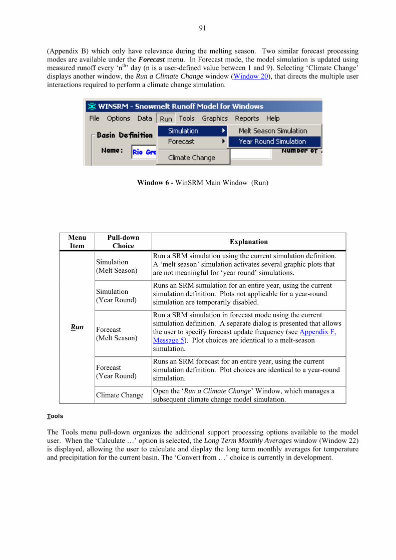
91

(Appendix B) which only have relevance during the melting season. Two similar forecast processing odes are available under the Forecast menu. In Forecast mode, the model simulation is updated using

measured runoff every ‘nth’ day (n is a user-defined value between 1 and 9). Selecting ‘Climate Change’ n a Climate Change window (Window 20

m

displays another window, the Ru ), that directs the multiple user teractions required to perform a climate change simulation. in

Window 6 - WinSRM Main Window (Run)

Menu Pull-down Explanation Item Choice

Simulation Run a SRM simulation using the current simulation definition.

(Melt Season) A ‘melt season’ simulation activates several graphic plots that are not meaningful for ‘year round’ simulations.

Simulation (Year Round)

Runs an SRM simulation for an entire year, using the current simulation definition. Plots not applicable for a year-round simulation are temporarily disabled.

Forecast

Run a SRM simulation in forecast mode using the current simulation definition. A separate dialog is presented that allows the user to specify forecast update frequency (see

(Melt Season) Appendix F,

Message 5). Plot choices are identical to a melt-season simulation.

Forecast (Year Round)

Runs an SRM forecast for an entire year, using the current simulation definition. Plot choices a

Run

re identical to a year-round simulation.

Climate Change Open the ‘Run a Climate Change’ Window, which manages a subsequent climate change model simulation.

Tools The Tools menu pull-down organizes the additional support processing options available to the model user. When the ‘Calculate …’ option is selected, the Long Term Monthly Averages window (Window 22) is displayed, allowing the user to calculate and display the long term monthly averages for temperature nd precipitation for the current basin. The ‘Convert from …’ choice is currently in development. a

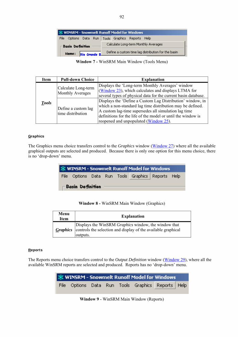
92

Window 7 - WinSRM Main Window (Tools Menu)

Item Pull-down Choice Explanation

Calculate Long-term Monthly Averages

Displays the ‘Long-term Monthly Averages’ window (Window 23), which calculates and displays LTMA for several types of physical data for the current basin database.

Tools Define a custom lag time distribution

Displays the ‘Define a Custom Lag Distribution’ window, in which a non-standard lag time distribution may be defined. A custom lag-time supersedes all simulation lag time definitions for the life of the model or until the window is reopened and unpopulated (Window 25).

Graphics The Graphics menu choice transfers control to the Graphics window (Window 27) where all the available graphical outputs are selected and produced. Because there is only one option for this menu choice, there is no ‘drop-down’ menu.

Window 8 - WinSRM Main Window (Graphics) Menu Item Explanation

Graphics lays the WinSRM Graphics window, the window that

controls the selection and display of the available graphical outputs.

Disp

Reports The Reports menu choice transfers control to the Output Definition window (Window 29), where all the available WinSRM reports are selected and produced. Reports has no ‘drop-down’ menu.

Window 9 - WinSRM Main Window (Reports)

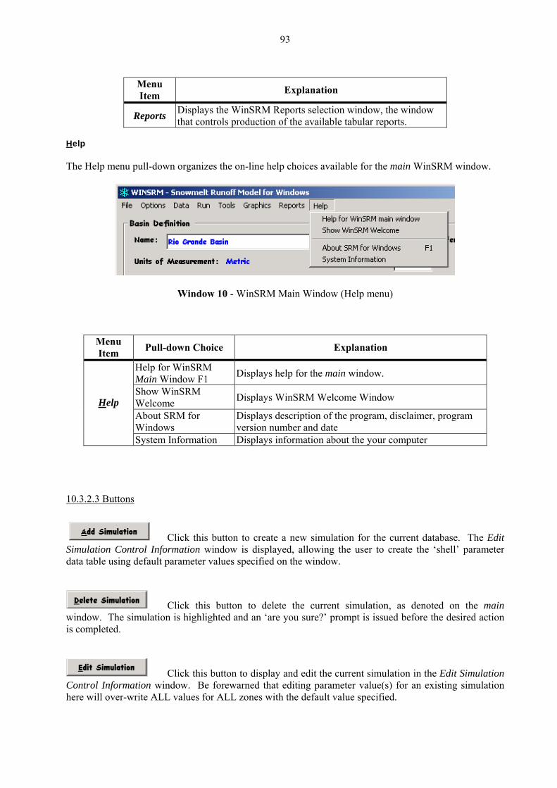
93

Menu Item Explanation

Reports Displays the WinSRM Reports selection windthat controls production of the available tabular reports.

ow, the window

Help The Help me n WinSRM window.

nu pull-down organizes the on-line help choices available for the mai

Window 10 - WinSRM Main Window (Help menu)


Help for WinSRM Main Window F1 Displays help for the main window.

Show WinSRM Welcome Displays WinSRM Welcome Window

About SRWindows

laimer, program M for Displays description of the program, discversion number and date

Help

System Information Displays information about the your computer

10.3.2.3 Buttons

Click this button to create a new simulation for the current database. The Edit Simulation Control Information window is displayed, allowing the user to create the ‘shell’ parameter data table using default parameter values specified on the window.

Click this button to delete the current simulation, as denoted on the main window. The simulation is highlighted and an ‘are you sure?’ prompt is issued before the desired action is completed.

Click this button to display and edit the current simulation in the Edit Simulation Control Information window. Be forewarned that editing parameter value(s) for an existing simulation here will over-write ALL values for ALL zones with the default value specified.

94

When theents and data entry

QuickHelp for Main Window button is clicked, context-sensitive help is displayed for structures within the main window that are subsequently clicked. The

or, and

10.3.2.4 Basin definition frame

the screen elemhelp data is displayed near the bottom of the window. While in help mode, a question mark (?) is displayed next to the cursor. No data can be entered and menu item and button functionality is suspended.Clicking the quickhelp button a second time will disable quickhelp, return to the standard cursenable data entry and other functionality.

The basin definition frame (Window 2) is a container for the physical characteristics that name, describe, and geo-locate the basin. This information is simulation neutral, that is, it applies for any simulation defined for the database. Two values NEVER change after their initial definition. Those values are ‘Units of Measurement’ and ‘Number of Zones’. All other descriptive variables in the frame may be changed at will. Generally, however, these variables will also be set only once. The zone definition grid table (Window 31) is the tool for entering and displaying the zonal characteristics of the current basin. Zone area and hypsometric mean elevation are the only values currently in use by the model. The remaining (aspect related) table cells are intended for possible future use as variations of the basic model algorithm are developed. The basin drainage area is automatically calculated using the areas entered in the zone definition grid table, and displayed (in bold blue) immediately underneath the table.

10.3.2.5 Basin simulation frame

The basin simulation frame (Window 2, Window 34) is a container used to display the individual simulation definition(s) that have been created for the current basin. Each line in the frame’s dat(

a grid Window 34) represents a unique simulation present in the database. Clicking on a grid line identifies at simulation as the ‘current’ simulation.

The ‘current’ simulation is an important property the software uses whenever any simulation-related

th

program functionality is accessed. For instance, if you click the window’s Edit Simulation button, the parameters for the current simulation are loaded into the Edit Simulation Control Information window. Each grid line constitutes a simulation, containing a variety of control information the model needs to initialize the physical and parameter data sets prior to simulation or climate-change processing. See Appendix D, SimulationIndex Table, for a description of these control columns. The ‘current’ simulation name is displayed below the basin simulations grid table in bold blue.

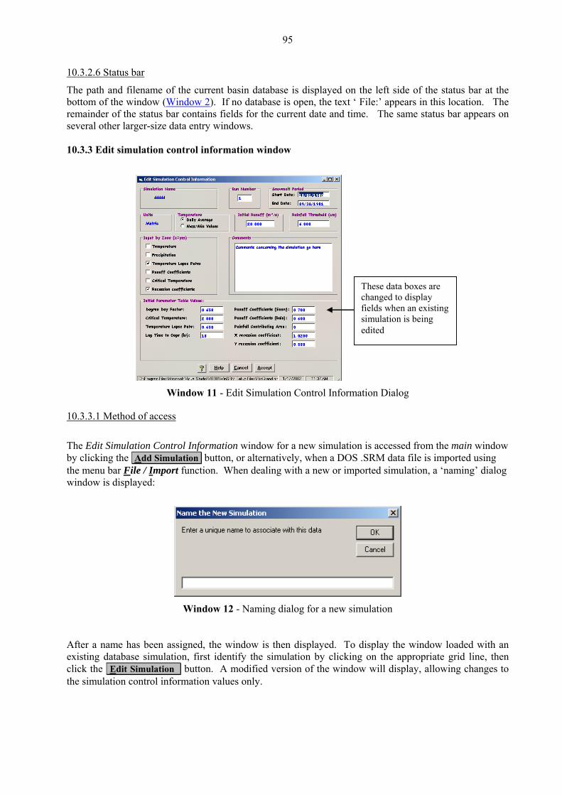
95

10.3.2.6 Status bar

The path and filename of the current basin database is displayed on the left side of the status bar at the bottom of the window (Window 2). If no database is open, the text ‘ File:’ appears in this location. The remainder of the status bar contains fields for the current date and time. The same status bar appears on several other larger-size data entry windows. 10.3.3 Edit simulation control information window

These data boxes are changed to display fields when an existing simulation is being edited

Window 11 - Edit Simulation Control Information Dialog

10.3.3.1 Method of access

Edit Simulation Control Information window for a new simulation is accessed from the main window Theby clicking the Add Simulation button, or alternatively, when a DOS .SRM data file is imported using the menu bar File / Import function. When dealing with a new or imported simulation, a ‘naming’ dialog

indow is displayed: w

Window 12 - Naming dialog for a new simulation

e has been assigned, the window is then displayed. To display the window loaded with an existing database simulation, first identify the simulation by clicking on the appropriate grid line, then

After a nam

click the Edit Simulation button. A modified version of the window will display, allowing changes to the simulation control information values only.

96

The Initial Parameter Values frame displays the parameter values for day #1, zone #1 as found in the simulation’s parameter table.

10.3.3.2 Purpose

The Edit Simulation Control Information window is used to define the initial parameter values and the control information for a new simulation. When a new simulation is created, a parameter table, named fter the simulation, is added to the database. The default parameters provided from this window are used

to populate the new table by assigning the parameter default value to all corresponding daily values for each zone for the entire simulation period. Once created, the simulation parameter table can be edited in more detail using the Edit Simulation Parameters window, by clicking the Data/Parameters on the main WinSRM window menu.

10.3.3.3 Buttons

a

Accept and apply the changes to the simulation and return to the Main Window.

Ignore any changes. Return control to the Main Window.

Display help window describing the window and its functions.

Toggle quickhelp comments related to the window elements/fields.


10.3.4 Edit {type of data} window

After a current simulat ulations data grid, the ariables and parameters used for the simulation may be displayed and edited using the Edit … Window. he appropriate window is accessed through the Main Window menu bar.

ion has been identified, by clicking on a row in the Basin SimvT

Window 13 - Display the Edit Basin Variables Dialog

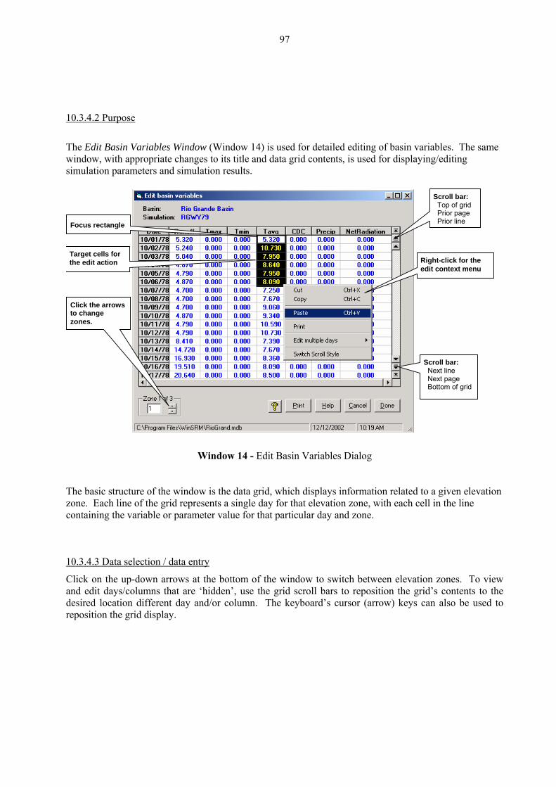
97

0.3.4.2 Purpose1

e e Th Edit Basin Variables Window (Window 14) is used for detailed editing of basin variables. The samwindow, with appropriate changes to its title and data grid contents, is used for displaying/editing simulation parameters and simulation results.

Scroll bar: Top of grid Prior page Prior line

Right-click for the edit context menu

Focus rectangle

Target cells for the edit action

Click the arrows to change zones.

Scroll bar: Next line Next page Bottom of grid

Window 14 - Edit Basin Variables Dialog

The basic structure of the window is the data grid, which displays information related to a given elevation zone. Each line of the grid represents a single day for that elevation zone, with each cell in the line containing the variable or parameter value for that particular day and zone.

10.3.4.3 Data selection / data entry

Click on the up-down arrows at the bottom of the window to switch between elevation zones. To view and edit days/columns that are ‘hidden’, use the grid scroll bars to reposition the grid’s contents to the desired location different day and/or column. The keyboard’s cursor (arrow) keys can also be used to reposition the grid display.

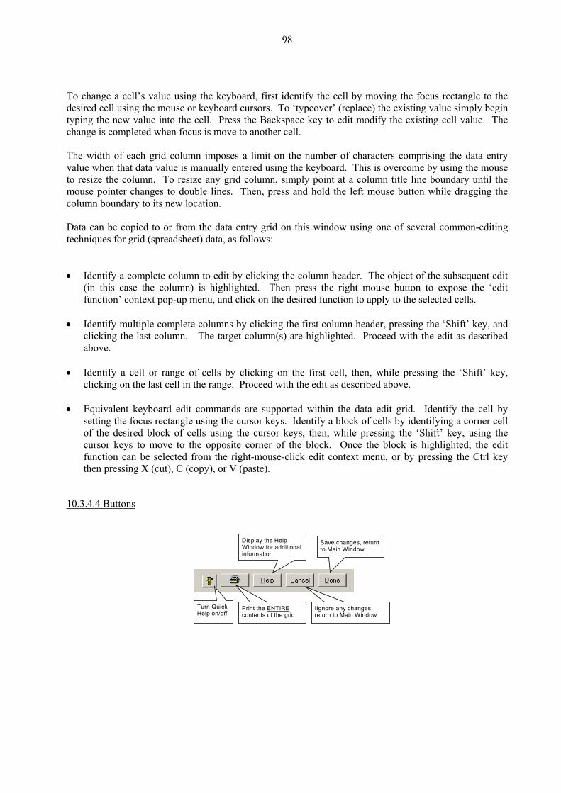
98

sing the keyboard, first identify the cell by moving the focus rectangle to the

poses a limit on the number of characters comprising the data entry value when that data value is manually entered using e keyboard. This is overcome by using the mouse to resize the column. To resize any olumn title line boundary until the mouse pointer changes to double lines. Then, press ouse button while dragging the

• Identify multiple complete columns by clicking the first column header, pressing the ‘Shift’ key, and clicking the last column. The target column(s) are highlighted. Proceed with the edit as described above.

• Identify a cell or range of cells by clicking on the first cell, then, while pressing the ‘Shift’ key,

clicking on the last cell in the range. Proceed with the edit as described above. • Equivalent keyboard edit commands are supported within the data edit grid. Identify the cell by

setting the focus rectangle using the cursor keys. Identify a block of cells by identifying a corner cell of the desired block of cells using the cursor keys, then, while pressing the ‘Shift’ key, using the cursor keys to move to the opposite corner of the block. Once the block is highlighted, the edit function can be selected from the right-mouse-click edit context menu, or by pressing the Ctrl key then pressing X (cut), C (copy), or V (paste).

10.3.4.4 Buttons

To change a cell’s value udesired cell using the mouse or keyboard cursors. To ‘typeover’ (replace) the existing value simply begin typing the new value into the cell. Press the Backspace key to edit modify the existing cell value. The change is completed when focus is move to another cell. The width of each grid column im

th grid column, simply point at a c

and hold the left mcolumn boundary to its new location. Data can be copied to or from the data entry grid on this window using one of several common-editing techniques for grid (spreadsheet) data, as follows: • Identify a complete column to edit by clicking the column header. The object of the subsequent edit

(in this case the column) is highlighted. Then press the right mouse button to expose the ‘edit function’ context pop-up menu, and click on the desired function to apply to the selected cells.

Save changes, return to Main Window

Display the Help Window for additional information

Print the ENTIRE contents of the grid

Turn Quick Help on/off

IIgnore any changes, return to Main Window

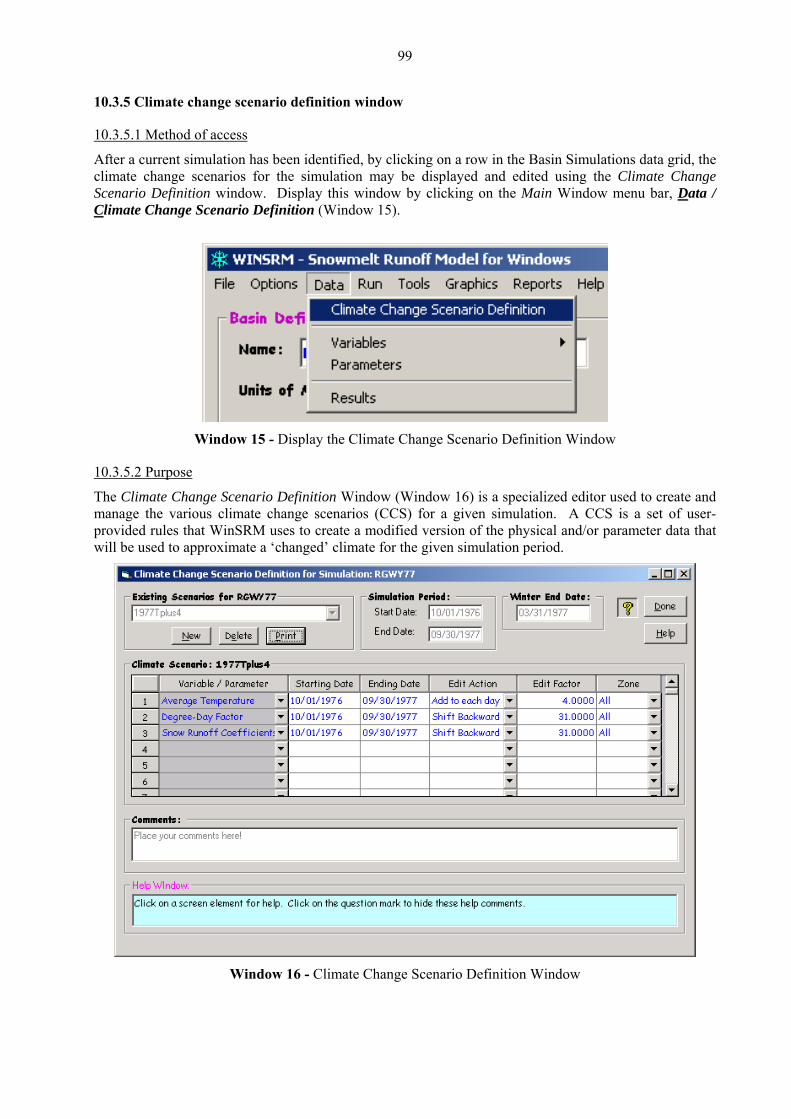
99

10.3.5 Climate change scenario definition window


After a current simulation has been identified, by clicking on a row in the Basin Simulations data grid, the lation may be displayed and edited using the Climate Change

Scenario Definition window. Display this window by clicking on the Main Window menu bar, Dclimate change scenarios for the simu

ata / Climate Change Scenario Definition (Window 15).

Window 15 - Display the Climate Change Scenario Definition Window

10.3.5.2 Purpose

The Climate Change Scenario Definition Window (Window 16) is a specialized editor used to create and manage the various climate change scenarios (CCS) for a given simulation. A CCS is a set of user-provided rules that WinSRM uses to create a modified version of the physical and/or parameter data that will be used to approximate a ‘changed’ climate for the given simulation period.

Window 16 - Climate Change Scenario Definition Window

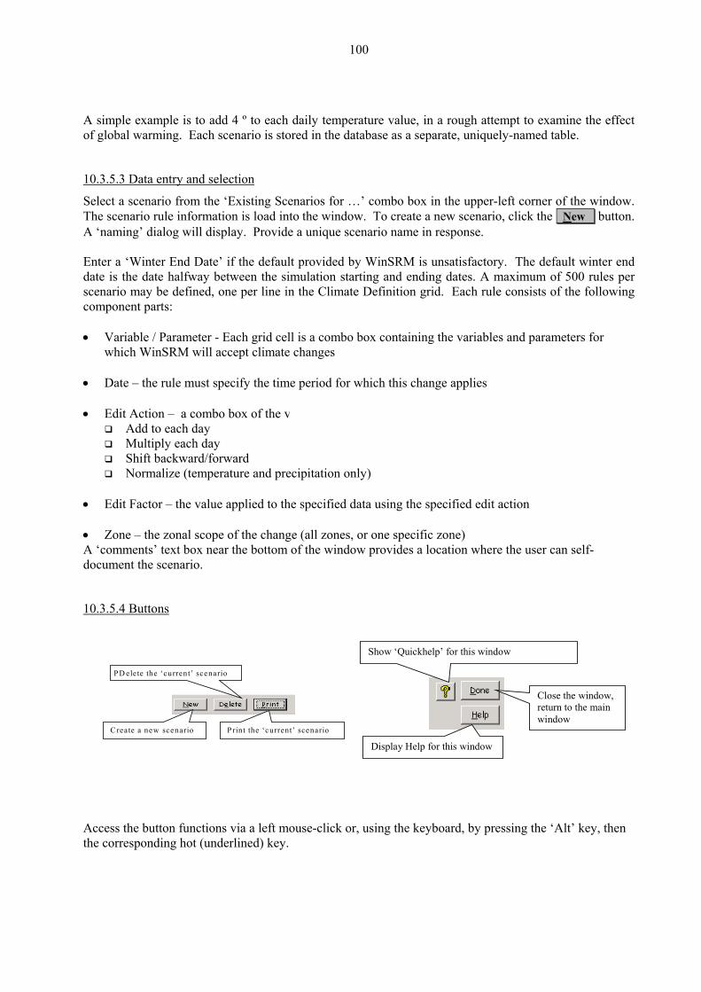
100

A simple example is to add 4 º to each daily temperature value, in a rough attempt to examine the effecof global warming. Each scenario is stored in the database as a separate, uniquely-named table.

t

10.3.5.3 Data entry and selection

Select a scenario from the ‘Existing Scenarios for …’ combo box in the upper-left corner of the window. The scenario rule information is load into the window. To create a new scenario, click the New button. A ‘naming’ dialog will display. Provide a unique scenario name in response.

nter a ‘Winter End Date’ if the default provE ided by WinSRM is unsatisfactory. The default winter end

limate changes

Multiply each day ward/forward

perature and precipitation only) • Edit Factor – the value applied to the specified data using the specified edit action • Zone – the zonal scope of the change (all zones, or one specific zone) A ‘comments’ text box near the bottom of the window provides a location where the user can self-document the scenario.

10.3.5.4 Buttons

date is the date halfway between the simulation starting and ending dates. A maximum of 500 rules per scenario may be defined, one per line in the Climate Definition grid. Each rule consists of the following component parts: • Variable / Parameter - Each grid cell is a combo box containing the variables and parameters for

which WinSRM will accept c • Date – the rule must specify the time period for which this change applies • Edit Action – a combo box of the valid edit actions available for the variable/parameter

Add to each day

Shift backNormalize (tem

Sh

P D elete the ‘current’ scenario

C reate a new scenario P rint the ‘current’ scenario

Display Help for this window

ow ‘Quickhelp’ for this window

Close the window,

ccess the button functions via a left mouse-click or, using the keyboard, by pressing the ‘Alt’ key, then

return to the main window

Athe corresponding hot (underlined) key.

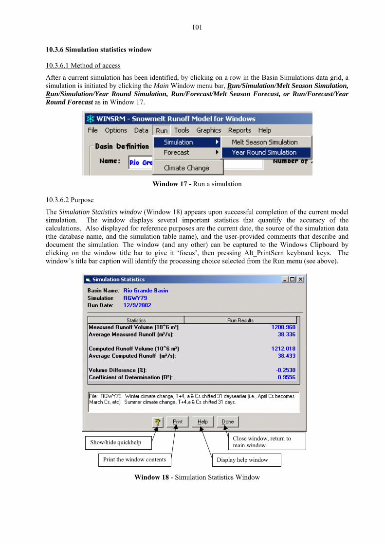
101

10.3.6 Simulation statistics window


After a current simulation has been identified, by clicking on a row in the Basin Simulations data grid, a e Main Window menu bar, Run/Simulation/Melt Season Simulation, simulation is initiated by clicking th

Run/Simulation/Year Round Simulation, Run/Forecast/Melt Season Forecast, or Run/Forecast/Year Round Forecast as in Window 17.

Window 17 - Run a simulation

Purpose10.3.6.2

ulation Statistics window (Window 18) appears upon successful completion of the current model s several important statistics that quantify the accuracy of the

The Simsimulation. The window displaycalculations. Also display(d clicking on the window title bar to give it ‘focus’, then pressing Alt_PrintScrn keyboard keys. The window’s title bar caption will identify the processing choice selected from the Run menu (see above).

ed for reference purposes are the current date, the source of the simulation data the database name, and the simulation table name), and the user-provided comments that describe and ocument the simulation. The window (and any other) can be captured to the Windows Clipboard by

Close window, return to main window

Display help window Print the window contents i d i

Show/hide quickhelp i i d

Window 18 - Simulation Statistics Window

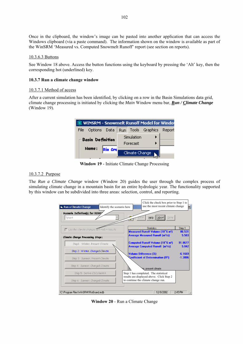
102

Once inWindowsthe WinS off’ report (see section on reports).

0.3.6.3 Buttons

the clipboard, the window’s image can be pasted into another application that can access the clipboard (via a paste command). The information shown on the window is available as part of RM ‘Measured vs. Computed Snowmelt Run

1

See Window 18 above. Access the button functions using the keyboard by pressing the ‘Alt’ key, then the corresponding hot (underlined) key

10


.

.3.7 Run a climate change window

Afclimate

ter a current simulation has been identified, by clicking on a row in the Basin Simulations data grid, change processing is initiated by clicking the Main Window menu bar, Run / Climate Change w 19).

(Windo

Window 19 - Initiate Climate Change Processing

Purpose10.3.7.2

a Climate Change window (Window 20) guides the user throughate change in a mountain basin for an entire hydrologic year. The functionality

The Run the complex process of simulating clim supported by ee areas: selection, control, and reporting.

this window can be subdivided into thr

Identify the scenario here Click the check box prior to Step 1 to use the most recent climate change

Step 1 has completed. The statistical results are displayed above. Click Step 2 to continue the climate change run.

Window 20 - Run a Climate Change

103

Selection – The first step in modeling climate change is to identify the climate change scenario that will control the process. A climate change scenario (See Climate Change Scenario Definition Window,

rio table) is a database table containing a set of rules for altering the original

the Existing Scenario Definition(s) dropdown ombo box, located in the upper left corner of the window. This combo box contains a list of all the

climate change scenarios that have been defined for use with the ‘current’ simulation. An alternative (to be discussed later in ate change run. This is accomplished by clicking the ‘Use the Climate Changes Defined in Results’ check-box. (Note

select a scenario from the combo box, as that is where WinSRM obtains the ‘Winter

tion step’ (Step 5), wherein climate-changed snow cover data is modeled. Each step is executed in sequence by clicking the ‘active’ button on the Climate Change Processing Steps frame. Reporting – as each processing step is completed, the Statistics data grid is updated to display the statistics resulting from the completion of the step (Steps 1,2,3,6 only). In addition to this reporting of simulation statistics, the user can access the main window’s plotting and reporting capabilities by clicking on the main window menu-bar (G

Appendix D, ClimateScenavariables and/or parameters used with a simulation to approximate a ‘changed-climate’. Included in the scenario is a ‘WinterEndDate’, which separates the simulation period into winter and a summer half-

ears. The scenario is identified by selecting an entry fromyc

this document) is to re-use the climate changes from an earlier clim

that you must stillEnd Date’ value needed during processing.) Control – After the scenario has been determined, the model is ready to begin processing. A ‘climate-change’ run is, in reality, four complete iterations through the model algorithms (Steps 1,2,3,6), one partial model execution (Step 4), and a ‘data genera

raphics or Reports)

10.3.7.3 Buttons

Toggle Quickhelp

Print statistics(after Step 6)

Display help window

Terminate the run, return to main window.

Return to main window.Enabled after step 6completes.

10.3.7.4 Processing steps controlled by the step buttons

table to form a temporary table

arameters that define

check box is hecked. When checked, the process of building the Results table is bypassed. The Results table built

Step 1: Winter, Present Climate Prior to a WinSRM simulation (with on exception), a copy of the pertinent physical data is queried from the database and combined with the current simulation’s parameter data named ‘Results’. There is one Results table per WinSRM database. Each simulation overwrites the existing table. After the Results table is created, companion columns to the variables and parameters that affect climate change are initialized using the associated ‘present climate’ values, and then modified under control of the rules found in the selected climate change scenario. These companion columns, identified with the ‘CC’ postfix in the column heading, represent the variables and pthe proposed changed-climate. The exception noted above occurs when the ‘Use the Climate Changes Defined in Results’ c

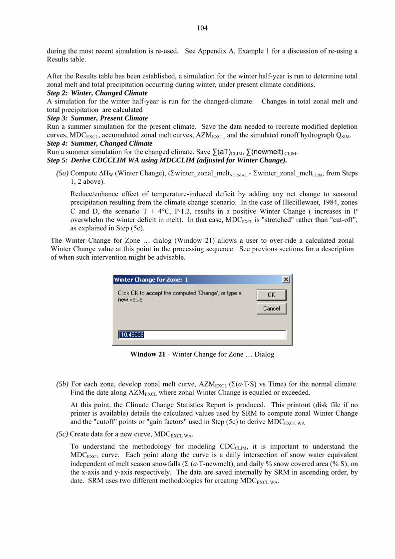
104

during the most recent simulation is re-used. See Appendix A, Example 1 for a discussion of re-using a Results table.

simulation for the winter half-year is run for the anged-climate. Changes in total zonal melt and tal precipitation are calculated tep 3: Summer, Present Climate

Run a summer simu modified depletion curves, MDC , accumulated zonal melt curves, AZMEXCL, and the simulated runoff hydrograph QSIM.

Changed Climate

Reduce/enhance effect of temperature-induced deficit by adding any net change to seasonal precipitation resulting from the climate change scenario. In the case of Illecillewaet, 1984, zones C and D, the scenario T + 4°C, P⋅1.2, results in a positive Winter Change ( increases in P overwhelm the winter deficit in melt). In that case, MDCEXCL is "stretched" rather than "cut-off", as explained in Step (5c).

The Winter Change for Zone … dialog (Window 21) allows a user to over-ride a calculated zonal Winter Change value at this point in the processing sequence. See previous sections for a description of when such intervention might be advisable.

After the Results table has been established, a simulation for the winter half-year is run to determine total zonal melt and total precipitation occurring during winter, under present climate conditions.

tep 2: Winter, Changed Climate SA chtoS

lation for the present climate. Save the data needed to recreateEXCL

Step 4: Summer, Run a summer simulation for the changed climate. Save ∑(aT)CLIM, ∑(newmelt) CLIM. Step 5: Derive CDCCLIM WA using MDCCLIM (adjusted for Winter Change).

(5a) Compute ∆HW (Winter Change), (Σwinter_zonal_meltNORMAL - Σwinter_zonal_meltCLIM, from Steps 1, 2 above).

Window 21 - Winter Change for Zone … Dialog

(5b) For each zone, develop zonal melt curve, AZMEXCL (Σ(a⋅T⋅S) vs Time) for the normal climate. Find the date along AZMEXCL where zonal Winter Change is equaled or exceeded.

At this point, the Climat . This printout (disk file if no used by SRM to compute zonal Winter Change

toff" points or "gain factors" used in Step (5c) to derive MDCEXCL WA

ethodology for modeling CDCCLIM, it is important to understand the MDCEXCL curve. Each point along the curve is a daily intersection of snow water equivalent independent of melt season snowfalls (Σ (a⋅T-newmelt), and daily % snow covered area (% S), on the x-axis and y-axis respectively. The data are saved internally by SRM in ascending order, by date. SRM uses two different methodologies for creating MDCEXCL WA.

e Change Statistics Report is producedprinter is available) details the calculated valuesand the "cu

(5c) Create data for a new curve, MDCEXCL WA.

To understand the m

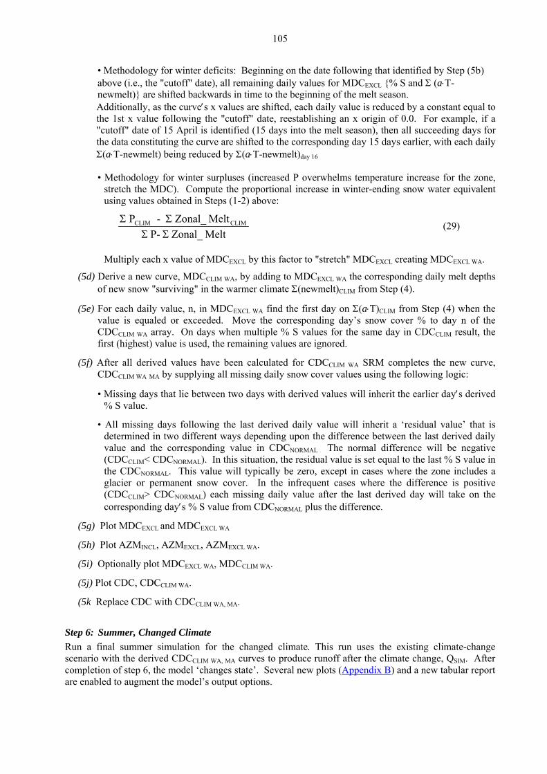
105

• Methodology for winter deficits: Beginning on the date following that identified by Step (5b) above (i.e., the "cutoff" date), all remaining daily values for MDCEXCL {% S and Σ (a⋅T-

d backwards in time to the beginning of the melt season.

e corresponding day 15 days earlier, with each daily Σ(a⋅T-n • Meth ne,

str c alent using

newmelt)} are shifteAdditionally, as the curve′s x values are shifted, each daily value is reduced by a constant equal to the 1st x value following the "cutoff" date, reestablishing an x origin of 0.0. For example, if a "cutoff" date of 15 April is identified (15 days into the melt season), then all succeeding days for the data constituting the curve are shifted to th

ewmelt) being reduced by Σ(a⋅T-newmelt)day 16

odology for winter surpluses (increased P overwhelms temperature increase for the zoh the MDC). Compute the proportional increase in winter-ending snow water equiv values obtained in Steps (1-2) above:

et

Σ ΣΣ ΣP- Zonal_ Melt

(29) P - Zonal_ MeltCLIM CLIM

Mu ti tretch" MDCEXCL creating MDCEXCL WA.

(5d) Deri e A the corresponding daily melt depths of new snow "surviving" in the warm CLIM from Step (4).

(5e) For ac y on Σ(a⋅T)CLIM from Step (4) when the value is equaled or exceeded. Move the corre n of the CDC L IM result, the first (highest) value is used, the rem

(5f) After all derived values have been calculated for CDCCLIM WA SRM completes the new curve, CDCCL sing the following logic:

• Missi e earlier day′s derived % S v

• All m a ‘residual value’ that is determined in two different ways depending upon the difference between the last derived daily va e negative (CDCCLIM< CDCNORMAL). In this situation, the residual value is set equal to the last % S value in the ne includes a glacier or permanent snow cover. In the infrequent cases where the difference is positive (CDC n the corresponding day′s % S value from CDCNORMAL plus the difference.

(5g) Plot M

A, MA.

Step 6: Summer, Changed Climate Run a final summer simulation for the changed climate. This run uses the existing climate-change scenario with the derived CDCCLIM WA, MA curves to produce runoff after the climate change, QSIM. After completion of step 6, the model ‘changes state’. Several new plots (Appendix B

l ply each x value of MDCEXCL by this factor to "s

v a new curve, MDCCLIM WA, by adding to MDCEXCL W

er climate Σ(newmelt)

e h daily value, n, in MDCEXCL WA find the first dasponding day’s snow cover % to day

IM WAC array. On days when multiple % S values for the same day in CDCCLaining values are ignored.

IM WA MA by supplying all missing daily snow cover values u

ng days that lie between two days with derived values will inherit thalue.

issing days following the last derived daily value will inherit

lu and the corresponding value in CDCNORMAL The normal difference will be

CDCNORMAL. This value will typically be zero, except in cases where the zo

CLIM> CDCNORMAL) each missing daily value after the last derived day will take o

DCEXCL and MDCEXCL WA

(5h) Plot AZMINCL, AZMEXCL, AZMEXCL WA.

(5i) Optionally plot MDCEXCL WA, MDCCLIM WA.

(5j) Plot CDC, CDCCLIM WA.

(5k Replace CDC with CDCCLIM W

) and a new tabular report are enabled to augment the model’s output options.

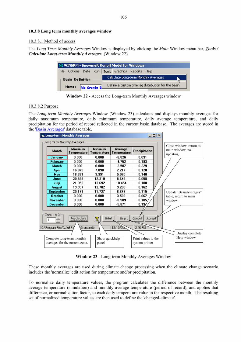
106

10.3.8 Long term


monthly averages window

The Long Term Monthly Averages Window is displayed by clicking the Main Window menu bar, Tools / Calculate Long-term Monthly Averages (Window 22).

Window 22 - Access the Long-term Monthly Averages window

10.3.8.2 Purpose

he Long-term Monthly Averages Window (Window 23) calculates and displayTd

s monthly averages for aily maximum temperature, daily minimum temperature, daily average temperature, and daily

rd reflected in the current basin database. The averages are stored in precipitation for the period of recothe 'Basin Averages' database table.

Update ‘BasinAverages” table, return to main window.

Close window, return to main window, no updating

Display complete Help window Compute long-term monthly

averages for the current zone. Print values to the system printer

Show quickhelp panel

Window 23 - Long-term Monthly Averages Window

These monthly averages are used during climate change processing when the climate change scenario includes the 'normalize' edit actio

o normalize daily temperature values, the program calculates the difference between the monthly average temperature (simulation) and monthly average temperature (period of record), and applies that difference, or normalization factor, to each daily temperature value in the respective month. The resulting set of normalized temperature values are then used to define the 'changed-climate’.

n for temperature and/or precipitation. T

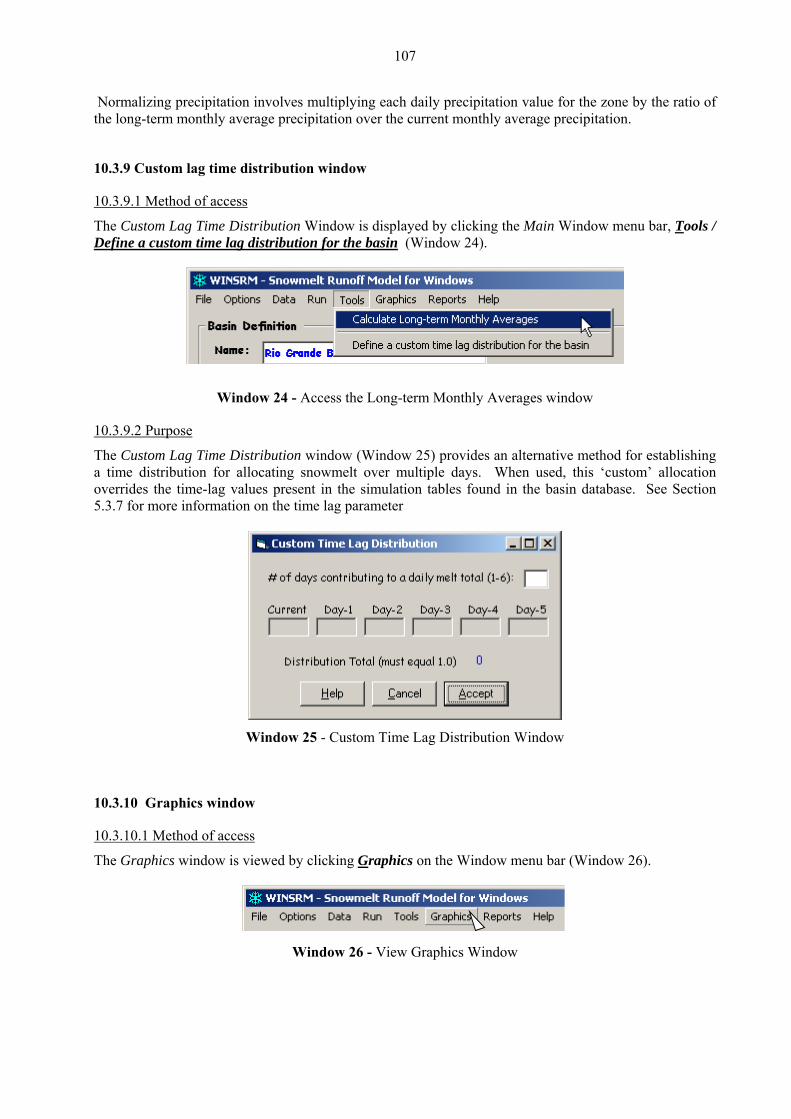
107

Normalizing precipitation involves multiplying each daily precipitation value for the zone by the ratio of the long-term monthly average precipitation over the current monthly average precipitation.

0.3.9 Cust


1 om lag time distribution window

The Cust m menu bar, To Lag Time Distribution Window is displayed by clicking the Main Window ools / Define a custom time lag distribution for the basin (Window 24).

Window 24 - Access the Long-term Monthly Averages window

10.3.9.2 Purpose

The Custom Lag Time Distribution window (Window 25) provides an alternative method for establishing a time distribution for allocating snowmelt over multiple days. When used, this ‘custom’ allocation overrides the time-lag values present in the simulation tables found in the basin database. See Section 5.3.7 for more information on the time lag parameter

Window 25 - Custom Time Lag Distribution Window

10.3.10 Graphics window


The Graphics window is viewed by clicking Graphics on the Window menu bar (Window 26).

Window 26 - View Graphics Window

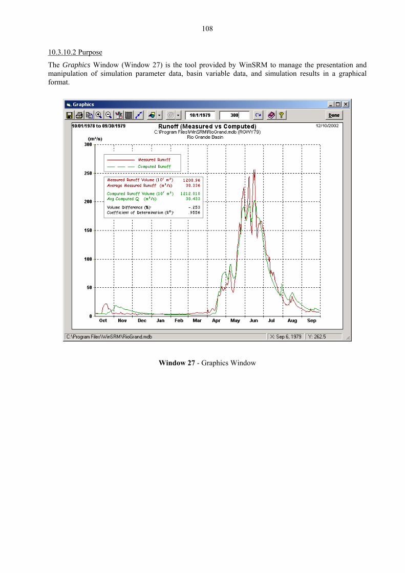
108

10.3.10.2 Purpose

dow (Window 27) is the tool provided by WinSRM to manage the presentation and mulation parameter data, basin variable data, and simulation results in a graphical

format.

The Graphics Winmanipulation of si

Window 27 - Graphics Window

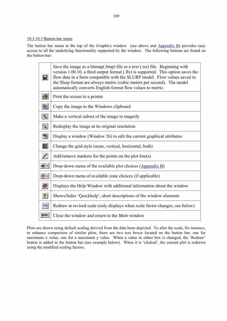
109

10.3.10.3 Button-bar menu

The button bar menu at the top of the Graphics window (see above and Appendix B) provides easy access to all the underlying functionality supported by the window. The following buttons are found on the button-bar:

version 1.00.10, a third output format (.flx) is supported. This option saves the flow data in a form compatible with the SLURP model. Flow values saved in the Slurp format are always metric (cubic meters per second). The model

Save the image as a bitmap(.bmp) file or a text (.txt) file. Beginning with

automatically converts English format flow values to metric.

Print the screen to a printer

Copy the image to the Windows clipboard

Make a vertical subset of the image to magnify

Redisplay the image at its original resolution

Display a window (Window 26) to edit the current graphical attributes

Change the grid style (none, vertical, horizontal, both)

Add/remove markers for the points on the plot line(s)

Drop-down menu of the available plot choices (Appendix B)

Drop-down menu of available zone choices (if applicable)

Displays the Help Window with additional information about the window

Shows/hides ‘Quickhelp’, short descriptions of the window elements

Redraw at revised scale (only displays when scale factor changes, see below)

Close the window and return to the Main window Plots are drawn using default scaling derived from the data been depicted. To alter the scale, for instance, to enhance comparison of similar plots, there are two text boxes located on the button bar, one for maximum x value, one for a maximum y value. When a value in either box is changed, the ‘Redraw’ button is added to the button bar (see example below). When it is ‘clicked’, the current plot is redrawn using the modified scaling factors.

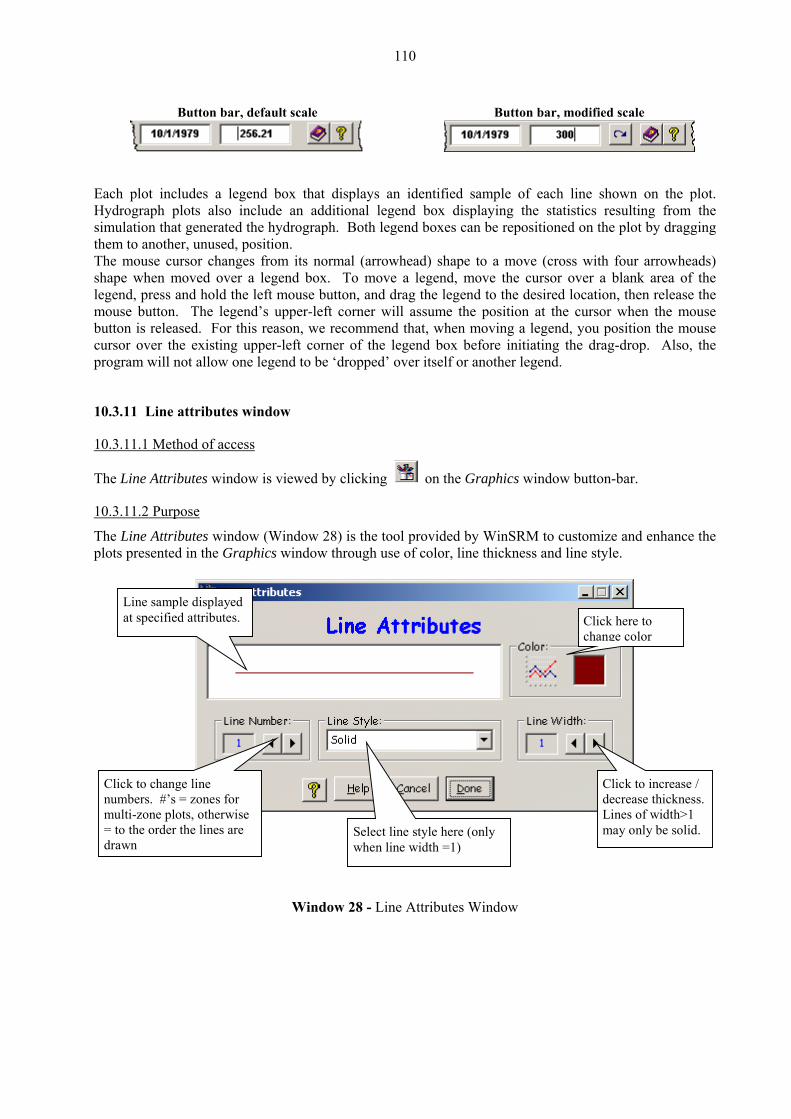
110

Button bar, default scale Button bar, modified scale

Each plot includes a legend box that displays an identified sample of each line shown on the plot. gend box displaying the statistics resulting from the

h legend boxes can be repositioned on the plot by dragging

a legend box. To move a legend, move the cursor over a blank area of the legend, press and hold the left mouse button, and drag the legend to the desired location, then release the

assume the position at the cursor when the mouse

ess

Hydrograph plots also include an additional lesimulation that generated the hydrograph. Botthem to another, unused, position. The mouse cursor changes from its normal (arrowhead) shape to a move (cross with four arrowheads) shape when moved over

mouse button. The legend’s upper-left corner will button is released. For this reason, we recommend that, when moving a legend, you position the mouse cursor over the existing upper-left corner of the legend box before initiating the drag-drop. Also, the program will not allow one legend to be ‘dropped’ over itself or another legend.

10.3.11 Line attributes window

10.3.11.1 Method of acc

The Line Attributes window is viewed by clicking on the Graphics window button-bar.

0.3.11.2 Purpose1

The Line Attributes window (Window 28) is the tool provided by WinSRM to customize and enhance the plots presented in the Graphics window through use of color, line thickness and line style.

Line sample displayed at specified attributes. Click here to

change color

Click to increase / decrease thickness. Lines of width>1 may only be solid.

Click to change line numbers. #’s = zones for multi-zone plots, otherwise = to the order the lines are drawn

Select line style here (only when line width =1)

Window 28 - Line Attributes Window

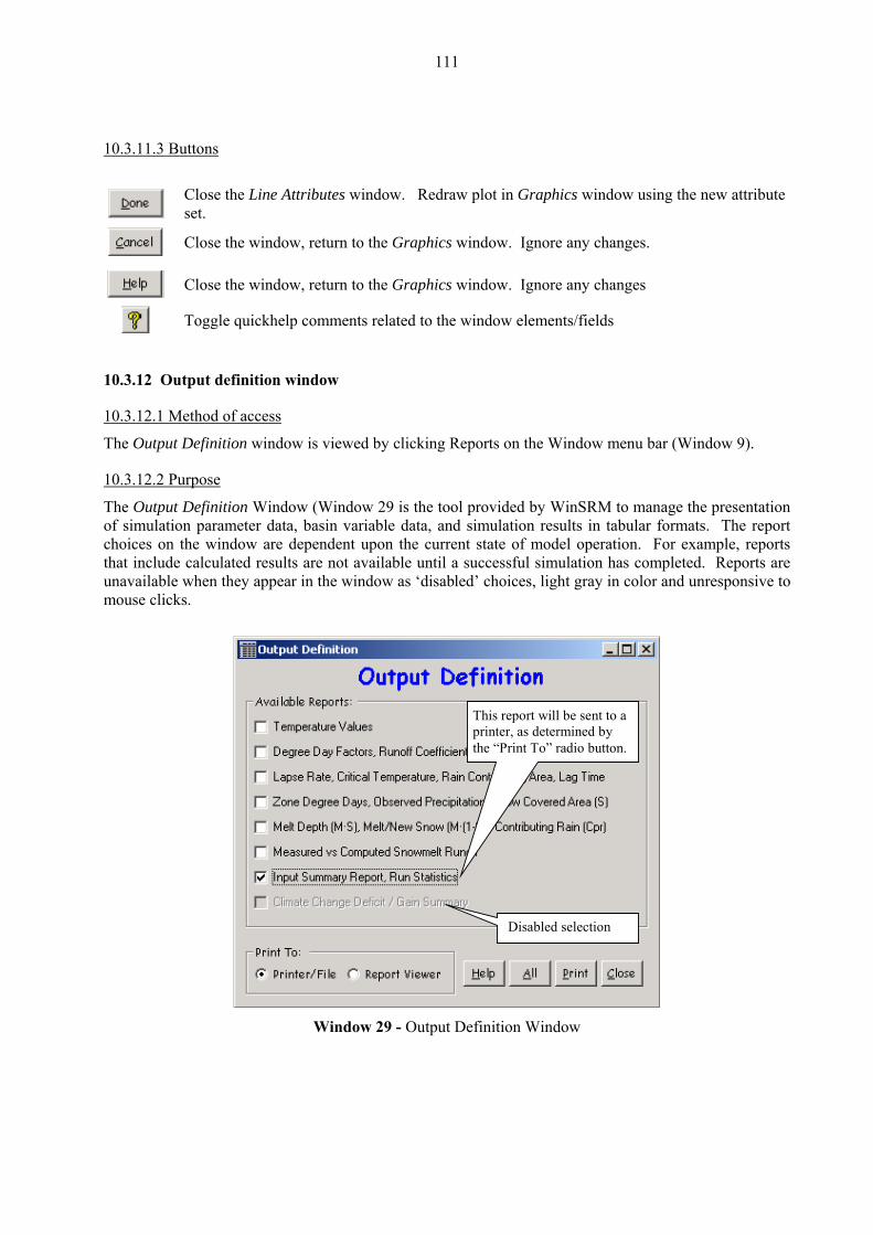
111

10.3.11.3 Buttons

set. Close the Line Attributes window. Redraw plot in Graphics window using the new attribute

Close the window, return to the Graphics window. Ignore any changes.

Close the window, return to the Graphics window. Ignore any changes

Toggle quickhelp comments related to the window elements/fields

10.3.12 Output definition window


The Output Definition window is viewed by clicking Reports on the Window menu bar (Window 9).

10.3.12.2 Purpose

The Output Definition Window (Window 29 is the tool provided by WinSRM to manage the presentation of simulation parameter data, basin variable data, and simulation results in tabular formats. The report choices on the window are dependent upon the current state of model operation. For example, reports that include calculated results are not available until a successful simulation has completed. Reports are unavailable when they appear in the window as ‘disabled’ choices, light gray in color and unresponsive to mouse clicks.

Disabled selection

This report will be sent to a printer, as determined by the “Print To” radio button.

Window 29 - Output Definition Window

112

10.3.12.3 Buttons

Click “Close” to close the Output Definition window and return to the WinSRM Main window.

This button caption toggles between View and Print, depending on which option button is selected, either Printer/File or Report Viewer.

If there are reports not checked, the button caption is “All”. Click “All” to check all the reports. When all the reports are checked, the caption toggles to “Reset”, which will clear all the check boxes.

Click “Help” to display the help text for the Output Definition Window

10.3.12.4 Available reports

Available reports shown in the Output Definition window are shown in the following summary

Report Name Description Current data description Lists the current user-input data.

Temperature values A a used with the current sim ation (average, max/min) is determined by the simulation’s temperature-type control value.

listing of the observed temperature datulation. The type of temperature inform

Degree-day factors Runoff coefficients

Parameters for the current simulation. This report is for one zone, or all zones, depending on the parameters’ distribution modifiers.

Lapse Rate Critical Temperature Lag Time

Parameters for the current simulation. This report is for one zone, or all zones, depending on the parameters’ distribution modifiers.

Zone Degree Days (DD) Observed Precipitation

snow cover for each elevation zone. DD values are calculated during a simulation. If chang

Snow Covered Area (S)

A table of the physical data for degree-day temperature, precipitation, and

es are made to the input data afterwards, the table will display ‘**’ for each DD value, and add a footnote to the table requesting a new simulation run.

Melt Depth (M·S) Melt/New Snow(M·(1-S)) Contributing Rain (Cpr)

A table displaying three important zonal values derived by the model during the simulation.

Measured vs. Computed Snowmelt Runoff

A table comparing daily basin runoff derived by the model with observed daily basin runoff, if available. Run statistics are included in this report.

Input Summary Report A summary of

Run Statistics

bimonthly values (1st, 16th) for 7 model parameters is printed for each zone in the basin. Run statistics are for the most current model simulation.

Climate Change Deficit / Gain Summary

The Climate Change Deficit/Gain Summary presents the computed values used to derive climate-affected snow cover.

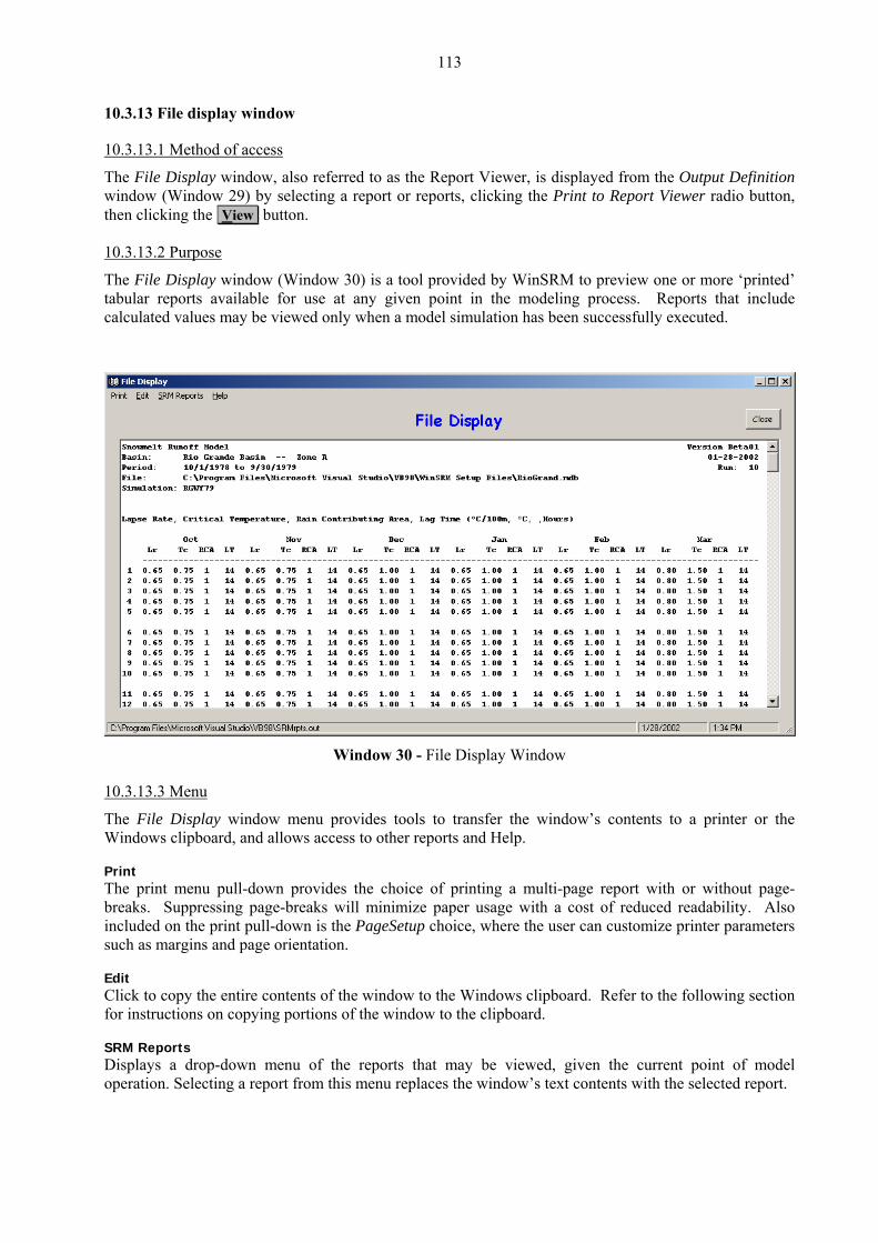
113

10.3.13 File display window


ile Display window, also referred to as the Report Viewer, is displayed The wi

F from the Output Definition ndow (Window 29) by selecting a report or reports, clicking the Print to Report Viewer radio button,

then clicking the View button.

10.3.13.2 Purpose

ile Display window (Window 30) is a tool provided by WinSRM to preview one or more ‘printed’ given point in the modeling process. Reports

The Ftabular reports available for use at any that include

ed only when a model simulation has been successfully executed. calculated values may be view

Window 30 - File Display Window

10.3.13.3 Menu

The File Display window menu provides tools to transfer the window’s contents to a printer or the ss to other reports and Help.

ters ins and page orientation.

d. Refer to the following section

Dis drop-down menu of the reports that may be viewed, given the current point of model ort.

Windows clipboard, and allows acce Print The print menu pull-down provides the choice of printing a multi-page report with or without page-breaks. Suppressing page-breaks will minimize paper usage with a cost of reduced readability. Also included on the print pull-down is the PageSetup choice, where the user can customize printer paramesuch as marg Edit

ipboarClick to copy the entire contents of the window to the Windows clfor instructions on copying portions of the window to the clipboard. SRM Reports

plays a operation. Selecting a report from this menu replaces the window’s text contents with the selected rep

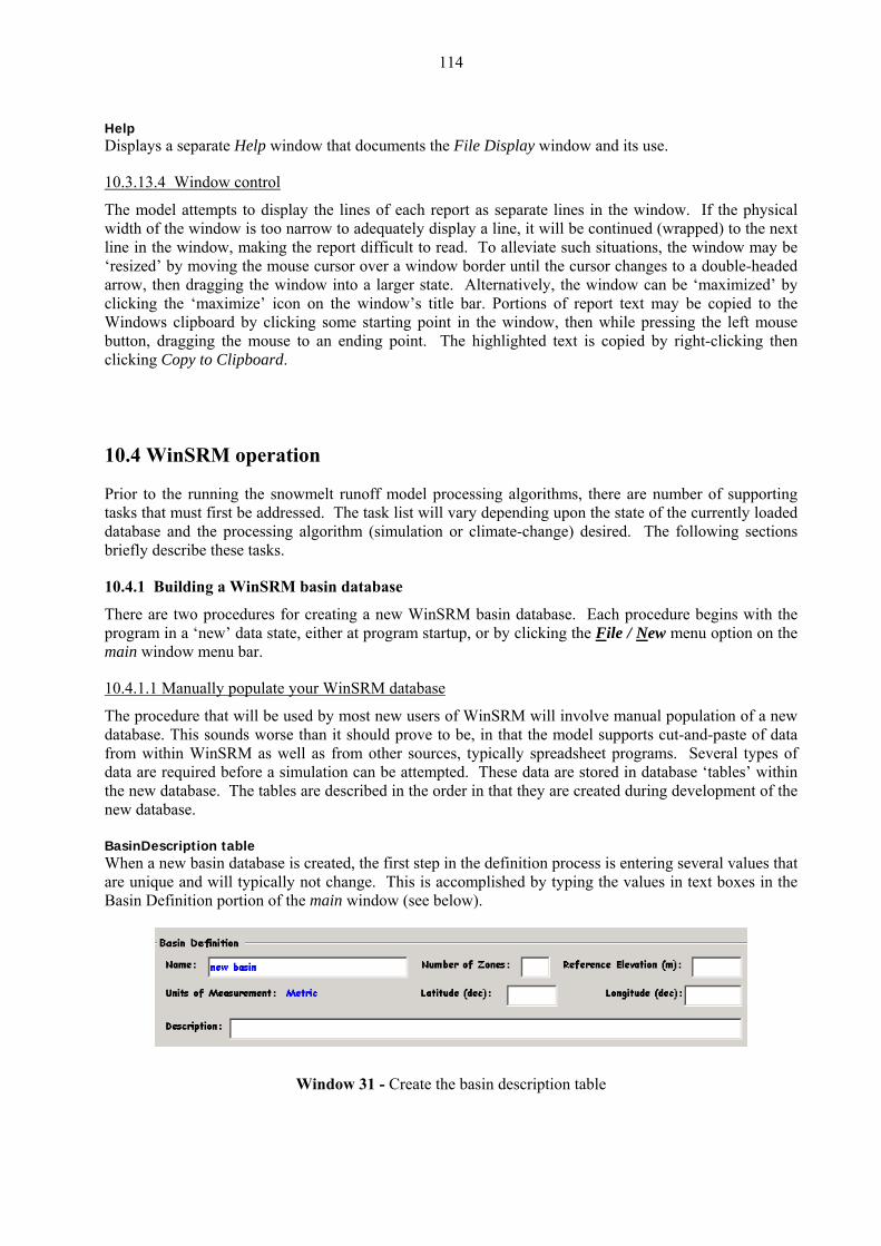
114

Help Displays a separate Help window that documents the File Display window and its use.

10.3.13.4 Window control

y the lines of each report as separate lines in the window. If the physical idth of the window is too narrow to adequately display a line, it will be continued (wrapped) to the next ne in the window, making the report difficult to read. To alleviate such situations, the window may be esized’ by moving the mouse cursor over a window border until the cursor changes to a double-headed

clickin f report text may be copied to the indows clipboard by clicking some starting point in the window, then while pressing the left mouse

10.4 W

databa n or climate-change) desired. The following sections riefly describe these tasks.

10.4.1

There egins with the rogram in a ‘new’ data state, either at program startup, or by clicking the F

The model attempts to displawli‘rarrow, then dragging the window into a larger state. Alternatively, the window can be ‘maximized’ by

g the ‘maximize’ icon on the window’s title bar. Portions oWbutton, dragging the mouse to an ending point. The highlighted text is copied by right-clicking then clicking Copy to Clipboard.

inSRM operation

Prior to the running the snowmelt runoff model processing algorithms, there are number of supporting tasks that must first be addressed. The task list will vary depending upon the state of the currently loaded

se and the processing algorithm (simulatiob

Building a WinSRM basin database

are two procedures for creating a new WinSRM basin database. Each procedure bp ile / New menu option on the

10.4.1.

main window menu bar.

1 Manually populate your WinSRM database

The procedure that will be used by most new users of WinSRM will involve manual population of a new database. This sounds worse than it should prove to be, in that the model supports cut-and-paste of data

ithin WinSRM as well as from other sources, typically spreadsheet programs. Several types of re required before a simulation can be attempted. These data are stored in database ‘tables’ within w database. The tables are described in the order in that they are created during d

from wdata athe ne evelopment of the ew database.

Whenare un not change. This is accomplished by typing the values in text boxes in the

asin Definition portion of the main window (see below).

n BasinDescription table

a new basin database is created, the first step in the definition process is entering several values that ique and will typically

B

Window 31 - Create the basin description table

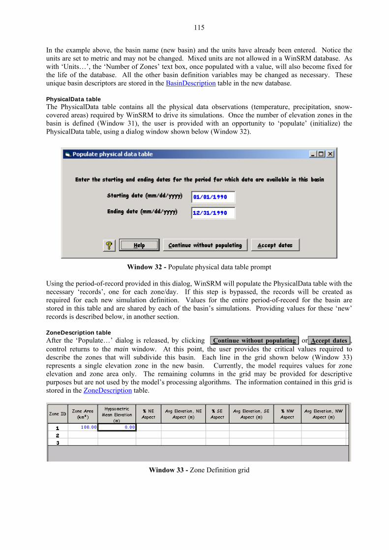
115

In the example above, the basin name (new basin) and the units have already been entered. Notice the re set to metric and may not be changed. Mixed units are not allowed in a WinSRM database. As nits…’, the ‘Number of Zones’ text box, once populated with a value, will a of the database. All the other basin definition variables may be changed

units awith ‘U lso become fixed for the life as necessary. These nique basin descriptors are stored in the BasinDescriptionu table in the new database.

PhysicalData table he PhysicalData table contains all the physical data observations (temperature, precipitation, snow-

PhysicalData table, using a dialog window shown below (Window 32).

Tcovered areas) required by WinSRM to drive its simulations. Once the number of elevation zones in thebasin is defined (Window 31), the user is provided with an opportunity to ‘populate’ (initialize) the

Window 32 - Populate physical data table prompt

Using the period-of-record provided in this dialog, WinSRM will populate the PhysicalData table with the

re ored in this table and are shared by each of the basin’s simulations. Providing values for these ‘new’

oneDescription table

necessary ‘records’, one for each zone/day. If this step is bypassed, the records will be created as required for each new simulation definition. Values for the entire period-of-record for the basin astrecords is described below, in another section.

ZAfter the ‘Populate…’ dialog is released, by clicking Continue without populating or Accept dates , control returns to the main window. At this point, the user provides the critical values required to describe the zones that will subdivide this basin. Each line in the grid shown below (Window 33)

presents a single elevation zone in the new basin. Currently, the model requires values for zone

purpo rid is ored in the ZoneDescription

reelevation and zone area only. The remaining columns in the grid may be provided for descriptive

ses but are not used by the model’s processing algorithms. The information contained in this gst table.

Window 33 - Zone Definition grid

116

SimulationIndex table name indicates, this table is the index of all the simulations that exist in the basin database. Each

g and ending date, etc.) required by

As itsrecord in the table represents a unique basin simulation, and stores the control information (name, run #, startin the model when the simulation is ‘run’. This information is

isplayed in the Basin Simulations grid on the WinSRM main window (Window 34). Each simulation dname must be unique in the database, as that value is used to create and access the simulation’s simulation parameter table, described below.

Simulation Parameter Table Each l

Window 34 - Basin Simulations grid

ine in the Basin Simulations grid represents a unique simulation parameter table stored in the t database, named using the value in the line’s Simulation Title grid cecurren ll (RGWY79 in the example

epicted in Window 34). The simulation table is the repository for the model parameters used by dWinSRM for that simulation. Each record in the table represents a parameter set for a given zone/day. Each n g the Add Simulation button on the main window. Once a ew simulation is created by clickinnIn

ame for the new simulation is provided (Window 12), control passes to the Edit Simulation Control formation

Once

dialog, where an initial set of simulation parameters is described.

a simulation parameter table has been defined, and indexed in the SimulationIndex table, the nese can be ‘Saved’, by clicking

w databa File/Save As.

port an existing DOS .SRM data file10.4.1.2 Im

ew (e se, the basin, zone, and physical variable database tables described in the next section re initialized using imported values, and a simulation parameter table

The simplest way to populate a WinSRM basin database is to import an existing .SRM data file created by an earlier DOS version of the SRM model software. When an existing .SRM file is imported into a

mpty) databana for the simulation is created using

to suppo that simulation. the imported simulation parameters. After the import finishes, the database is adequately populated

rt model processing of

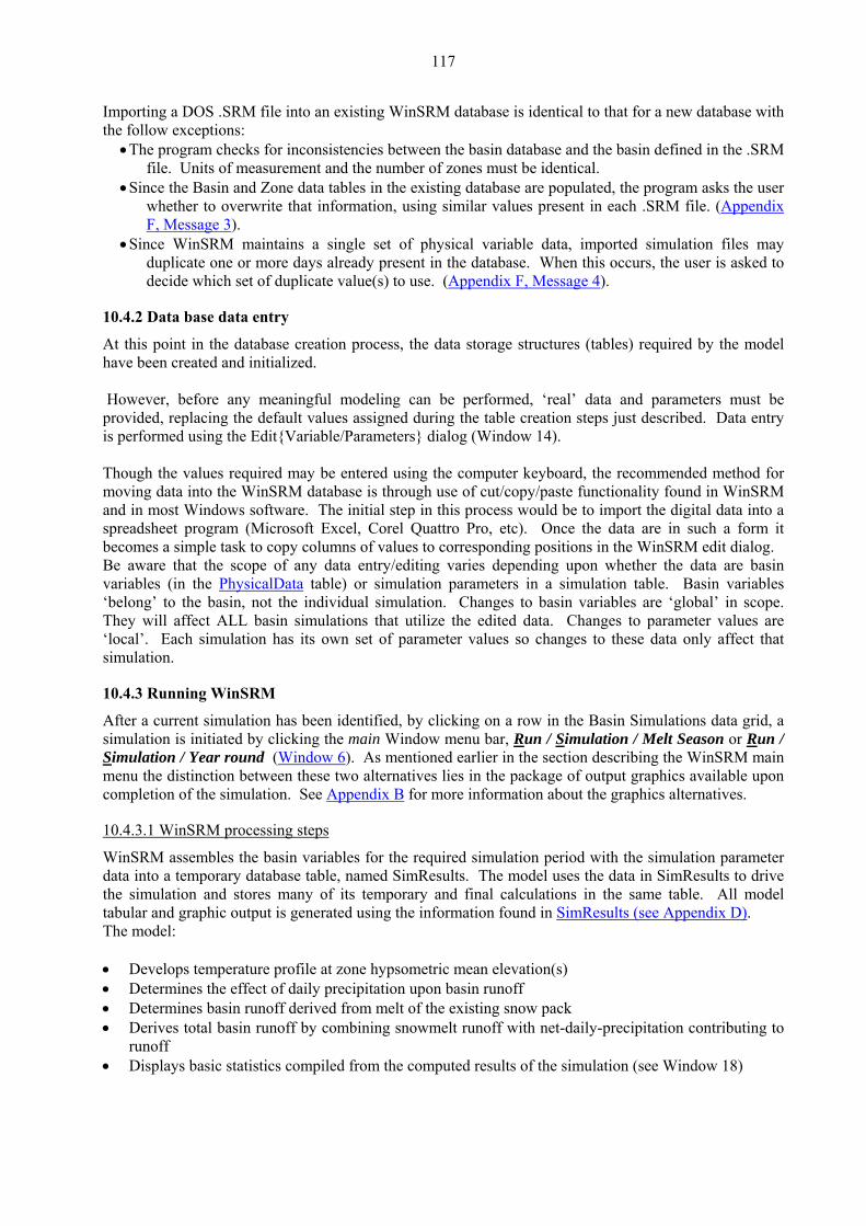
117

Importing a DOS .SRM file into an existing WinSRM database is identical to that for a new database with the follow exceptions:

es between the basin database and the basin defined in the .SRM ber of zones must be identical.

• Since the Basin and Zone data tables in the existing database are populated, the program asks the user

• The program checks for inconsistencifile. Units of measurement and the num

whether to overwrite that information, using similar values present in each .SRM file. (Appendix F, Message 3).

WinSRM maintains a single set of physical variable data, imported simulation files may duplicate one or more days alread

• Since y present in the database. When this occurs, the user is asked to

decide which set of duplicate value(s) to use. (Appendix F, Message 4).

10.4.2

At thi t in the database creation process, the data storage structures (tables) required by the model ave been created and initialized.

Howe can be performed, ‘real’ data and parameters must be e table creation steps just described. Data entry

ed using the Edit{Variable/Parameters} dialog (Window 14).

Thoug tered using the computer keyboard, the recommended method for oving data into the WinSRM database is through use of cut/copy/paste functionality found in WinSRM

becomBe aw ending upon whether the data are basin ariables (in the PhysicalData

Data base data entry

s poinh

ver, before any meaningful modelingprovided, replacing the default values assigned during this perform

h the values required may be enmand in most Windows software. The initial step in this process would be to import the digital data into a spreadsheet program (Microsoft Excel, Corel Quattro Pro, etc). Once the data are in such a form it

es a simple task to copy columns of values to corresponding positions in the WinSRM edit dialog. are that the scope of any data entry/editing varies dep

v table) or simulation parameters in a simulation table. Basin variables

They ‘local’ h

ula

After simula ing the main Window menu bar, R

‘belong’ to the basin, not the individual simulation. Changes to basin variables are ‘global’ in scope. will affect ALL basin simulations that utilize the edited data. Changes to parameter values are . Each simulation has its own set of parameter values so changes to t ese data only affect that tion. sim

10.4.3 Running WinSRM

a current simulation has been identified, by clicking on a row in the Basin Simulations data grid, a tion is initiated by click un / Simulation / Melt Season or Run /

Simulation / Year round (Window 6). As mentioned earlier in the section describing the WinSRM main ble upon

ompletion of the simulation. See Appendix Bmenu the distinction between these two alternatives lies in the package of output graphics availac for more information about the graphics alternatives.

10.4.3.1 WinSRM processing steps

M assembles the basin variables for the requiWd

inSR red simulation period with the simulation parameter

tabular esults (see Appendix D)

ata into a temporary database table, named SimResults. The model uses the data in SimResults to drive the simulation and stores many of its temporary and final calculations in the same table. All model

and graphic output is generated using the information found in SimR . he model:

• D Determ

ru• Displays basic statistics compiled from the computed results of the simulation (see Window 18)

T

evelops temperature profile at zone hypsometric mean elevation(s) ines the effect of daily precipitation upon basin runoff •

• Determines basin runoff derived from melt of the existing snow pack • Derives total basin runoff by combining snowmelt runoff with net-daily-precipitation contributing to

noff

118

EFERENCES 11. R

, Department of Geography, Univ. of Zurich, Zurich,

of satellite snow Water Resources,

Carlson, T. N. & Bunce, J. A. (1991) The effect of In: Salt Lake City,

Cronshey, R. G., R. T. Roberts, & Miller N. (

Gyalistras, D., H. von Storch, A. Fischlin, M. Benist

Climate Research Vol. 4 , pp 167-189

11.1 General references

Bahr, D.B., M.F. Meier, S.D. Peckham (1997) The Physical Basis of Glacier Volume-Area Scaling. Journal

of Geophysical Research, Vol. 102, No B9, pp 20355-20362. Baumgartner, M. F. (1987) Schneeschmelz-Abflusssimulationen basierend auf Schneeflächenbes-

timmungen mit digitalen Landsat-MSS and NOAA-AVHRR Daten. (Snowmelt runoff simulations based on snow cover mapping using digital Landsat-MSS and NOAA-AVHRR data), German version: Remote Sensing Serie, 11Switzerland. English summary: Tech. Report HL-16, USDA, Agricultural Research Service, Hydrol. Laboratory, Beltsville, MD, USA.

Baumgartner, M. F & Rango, A. (1995) A microcomputer-based alpine snow cover analysis system.

Photogramm. Engng, 61(12), 1475-1486.

forecasts in an Alpine catchment Baumann, R., Burkart, U. & Seidel, K. (1990) Runoff cover monitoring. Proc. International Symp. on Remote Sensing and International Association of Hydrogeologists, Enschede, The Netherlands, 181-190.

Becker, A. & Serban, P. (1990) Hydrological models for water resources system design and operation.

Operational. Hydrol. Report 34, WMO, Geneva, Switzerland.

Brüsch, W. (1996) Das Snowmelt Runoff Model ETH (SRM-ETH) als universelles Simulations und Prognosesystem von Schneeschmelz-Abflussmengen. (The Snowmelt Runoff Model ETH as a universal simulation and forecast system for snowmelt runoff) (in German), Remote Sensing Series27, Remote Sensing Laboratories RSL, University of Zurich, Zurich, Switzerland.

atmospheric carbon dioxide doubling on transpiration.

Proc. American Meteorological Society, Special Session on Hydrometeorology, Utah, USA, 196-199.

1985) Urban Hydrology for Small Watersheds (TR-55

Revised). Proc. ASCE Hydraulic Division Specialty Conference, Orlando, Florida, USA. Gifford, R. M. (1988) Direct effects of CO2 concentrations on vegetation. In: Greenhouse Planning for

Climate Change (ed. by G.L Pearlman), CSIRO, Melbourne, Australia, 506-519.

on (1994) Linking GCM-Simulated Climatic Changes to Ecosystem Models: Case Studies of Statistical Downscaling in the Alps,

119

Higuchi, K., Ageta, Y., Yasunari T. & Inoue, J. (1982) Characteristics of precipitation during the monsoon season in high-mountain areas of the Nepal Himalaya. In: Hydrological Aspects of Alpine and High Mountain Areas, (Proc. Exeter Symposium), IAHS Publ. no. 138, 21-30.

M VS FORTRAN Application Programming: Language Reference, GC26-3986-3. March (1983), 111-

Jaccar .

WMO,

artinec, J. (1970) Study of snowmelt runoff process in two representative watersheds with different

Martin 54.

ments, IAHS Symposium in Oxford, 1980, IAHS Publ. No. 129, pp. 239-246.

Martin a), vol. II, John Wiley & Sons, London, 249-290.

Martin and Glacier Variations (Proc. Baltimore Symp.), IAHS Publ. no. 183, 19-28.

artinec, J. & Rango, A. (1989): Merits of statistical criteria for the performance of hydrological models.

Martin . NASA

Reference Publ. 1100, Washington, D.C., USA.

Hall, D. K. & Martinec, J. (1985) Remote Sensing of Ice and Snow. Chapman & Hall Ltd., London - New

York.

IB112.

d, C. (1982) Recession coefficient formula, Personal communication Klemes, V. (1985) Sensitivity of water resources systems to climate variations. WCP Report 98,

Geneva, Switzerland. Kotlyakov, V. M. & Krenke, A. N. (1982) Investigations of the hydrological conditions of alpine regions by

glaciological methods. In: Hydrological Aspects of Alpine and High-Mountain Areas (Proc. Exeter Symposium), IAHS Publ. no. 138, 31-42.

Martinec, J. (1960) The degree-day factor for snowmelt runoff forecasting. IUGG General Assembly of

Helsinki, IAHS Commission of Surface Waters, IAHS Publ. no. 51, 468-477.

Melevation range. IAHS-Unesco Symp., Wellington, New Zealand., IAHS Publ. no. 96, 29-39.

ec, J. (1975) Snowmelt-Runoff Model for stream flow forecasts. Nordic Hydrol. 6(3), 145-1 Martinec, J. (1980) Snowmelt-Runoff Forecasts based on Automatic Temperature Measure

ec, J. (1985) Time in hydrology. In: Facets of Hydrology (ed. by J. C. Rodd

ec, J. (1989) Hour-to-hour snowmelt rates and lysimeter outflow during an entire ablation period. In: Snow Cover

Martinec, J. & Rango, A. (1986) Parameter values for snowmelt runoff modelling. J. Hydrol. 84, 197-

219.

MWat. Resour. Bull. 25(20), 421-432.

ec, J., Rango, A. & Major, E., 1983: The Snowmelt-Runoff Model (SRM) User's Manual

120

Martinec, J., Rango, A. & Roberts, R. (1994) The Snowmelt Runoff Model (SRM) User′s Manual (ed. by M. F. Baumgartner). Geographica Bernensia, P 29, Department of Geography, Univ. of Berne, Berne, Switzerland.

ash, L.L & Gleick, J.A. (1991) Sensitivity of streamflow in the Colorado basin to climatic changes. J.

ango, A. & Martinec, J. (1988) Results from international intercomparisons of snowmelt runoff model

Rango

enhagen, Denmark, 233-246.

ango, A. & Martinec, J. (1997) Water storage in mountain basins from satellite snow cover monitoring.

Rango, A. & van Katwijk, V. (1990) Development and testing of a snowmelt runoff forecasting technique.

Wat. Resour. Bull. 26(1), 135-144.

Shafe South Fork Rio Grande and Conejos River in Colorado. AgRISTARS Report CP-G1-

04072, Goddard Space Flight Center, Greenbelt, MD, USA.

ilson, W. T. (1941) An outline of the thermodynamics of snow-melt. Trans. Am. Geophys. Union, Part

WMO ( 3, WMO,

Geneva, Switzerland.

WMO (1992) Simulated real-time intercomparison of hydrological models. Operational Hydrol. Report 38, WMO, Geneva, Switzerland.

Martinec, J. & Rango, A. (1995) Seasonal runoff forecasts for hydropower based on remote sensing.

Proc. Western Snow Conf., Reno/Sparks, Nevada, USA, 10-20.

NHydrol. 125, 221-241.

Rperformance. Proc. 45th Annual Eastern Snow Conference, Lake Placid, New York, USA, 121-128.

, A. & Martinec, J. (1994) Areal extent of seasonal snow cover in a changed climate. Nordic Hydrol. 25, Munksgaard, Cop

Rango, A. & Martinec, J. (1995) Revisiting the degree-day method for snowmelt computation. Wat.

Resour. Bull. 31(4), 657-669.

RIn: Remote Sensing and Geographic Information Systems for Design and Operation of Water Resources Systems (ed. by M. F. Baumgartner, G. A. Schultz & A. I. Johnson), Proc. 5th Scientific Assembly of IAHS, Rabat, Morocco, IAHS Publication no. 242, 83-91.

r, B. A., Jones, E. B. & Frick, D. M. (1981) Snowmelt Runoff Simulations Using the Martinec-Rango Model on the

Soil Conservation Service (1986) "Urban Hydrology for Small Watersheds". Tech. Release 55 (2nd Edition).

W1, 182-195.

1986) Intercomparison of Models of Snowmelt Runoff. Operational Hydrol. Report 2

121

11.2 Specific references for Table 1

[1] Aschenbrenner, B., (1998). Snowmelt Runoff Technical

[5] Baumgartner, M. F., Spreafico, M. & Weiss, H. W., (2001) Operational snowmelt runoff forecasting in

PhD thesis, University of

[7] Baumgartner, M. F. & Rango, A., (1995). A Microcomputer-Based Alpine Snow-Cover Analysis 61

[8] Bedford, D., (1996). Data on Kafirnigan, Vakhsh, Pyandzh. Personal communication, 1996.

[10] Burn, D. E. & McBea, E. A., (1982). River Meeting

[11] Dey, B., Sharma, V. K., & Rango, , Vol. 20 : pp. 167-178.

Model applications in the Otztal (Austria).

Report, NN, 1998. Presentation at the Fourth Snowmelt Runoff Model Workshop held at the University of Berne, Switzerland.

[2] Azzouz, A., (1989). Martinec Rango Snowmelt Runoff Model applied to the Tillouguit Basin of Morocco. Master’s Thesis, South Dakota School of Mines and Technology, Rapid City, South Dakota, USA.

[3] Bagchi, A. K., (1983). Generation of the snowline. Photogrammetric Engineering and Remote

Sensing, Vol. 49(12): pp. 1679-1689.

[4] Baumgartner, M. F., (2002). Runoff in Pskem, Chatkal, Angren, Naryn, Karadarya, Vaksh, Zerafshan. Personal communication, 2002.

the Central Asian mountains. In Remote Sensing and Hydrology 2000. Proceedings of the Santa Fe Symposium, April 2000, IAHS Publ. No. 267 : pp. 66-71.

[6] Baumgartner, M. F., (1987). Schneeschmelz-Abflusssimulationen basierend auf Schneeflächen-

bestimmungen mit digitalen Landsat-MSS- und NOAA/AVHRR-Daten. Zürich, 1987. Referent: H. Haefner -Gutachter: K. Seidel.

System (ASCAS). Photogrammetric Engineering and Remote Sensing, Vol. No. (12) : pp. 1475-1486, December 1995.

[9] Boyer, E. W., (1990). Martinec and Rango's Snowmelt Runoff Model Applied to the Upper Yakima

River. Personal Communication, 1990.

flow forecasting model for the Sturgeon River. In of the American Geophysical Union, Fall 1982, San Francisco, 1982.

A., (1989). A Test of Snowmelt Runoff Model for a Major River

Basin in Western Himalayas. Nordic Hydrology [12] Dincer, T., Payne, B., Martinec, J., Tongiorgi, E., & Florkowski, T., (1970). Snowmelt runoff from

measurements of Tritium and Oxygen-18. Water Resources Research (AGU), Vol. 6, pp. 110-124.

122

[13] Escobar, C. F., Bales, R., & Pozo, V., (1998). Aplicación de un modelo de derretimiento de nieves (SRM 3.2) usando Sistemas de Información Geográfica (SIG) e imagines Landsat y NOAA. Personal Communication, 1998.

[14] Escobar, C. F. & Carin, C., (1997). Balance de Masa en el Glaciar Echaurren Norte, 1975 a 1992.

Resultados preliminares". D.G.A., H.A. y G., 97/1). Complemento No 1, años 1993-1996,1997.

H

6] Ehrler, C., (1998). Klimaanderung und alpine Schneedecke-Auswirkungen auf das Abflussregime am

[18] F

[20] G Personal Communication, 1996.

2] Gómez-Landesa, E. & Rango, A., (2002). Operational Snowmelt Runoff Forecasting in the Spanish

[23] G proved Snow Cover Remote Sensing for

Snowmelt Runoff Forecasting. In Remote Sensing and Hydrology 2000. Proceedings of the Santa

4] Gómez-Landesa, E., (1997). Evaluación de Recursos de Aqua en Forma de Nieve

[15] Escobar, C. F., (1992). Aplicacion del modelo "SRM 3-11" en cuencas de los Andes Centrales. In

Segundas Jornadas de Hidráulica Francisco Javier Domínguez, pages 283-295. Departamento de idrología, Ministerio de Obras Públicas, Santiago, Chile, Noviembre 1992.

[1Beispiel des Einzugsgebiets 'Rhein-Felsberg'. vdf Hochschulverlag an der ETH Zürich, NFP 31 Schlussbericht edition, 1998. 117 Seiten.

[17] Ferguson, R.I., (1984). Magnitude and modelling of snowmelt runoff in the Cairngorm mountains,

Scotland. Hydrological Sciences Journal, Vol. 29(1) pp. 49-62.

itzharris, B., (1991). Runoff. Personal Communication. [19] Galarraga, R., (1997). Runoff. Personal Communication.

arr, T., (1996). Runoff (Geehi River, Australia). [21] Gómez-Landesa, E., (2002). Snowmelt Runoff Model Worldwide Applications, Personal

Communication: International Snowmelt Forecast Seminar, U.S. AID Central Asia Natural Resources Management Project (NRMP). Tashkent, Uzbekistan, June 2002.

[2Pyrenees using the Snowmelt Runoff Model. Hydrological Processes, Vol. No. 16 : pp. 1583-1591.

ómez-Landesa, E., Rango, A., & Hall, D. K., (2001). Im

Fe Symposium, April 2000, IAHS Publication No. 267, pp. 61-65.

[2medianteTeledetección usando Satelites de la Serie NOAA (Estimation of snow water resources using remote sensing with NOAA satellites). Ph.D. Thesis, ETSICCP, Universidad Politécnica de Madrid, Spain, February 1997.

[25] Herrmann, A. & Rau, R. G., (1984). Snow cover stores and winter runoff behaviour of a small basin

in the German highlands. In Proceedings IUFRO Workshop on Snow Hydrologic Research in Central Europe, number 7, Hannoversch-Münden: Deutscher Verband für Wasserwirtschaft und Kulturbau, Bonn, Germany.

123

[26] Ishihara, K., Inoue, M., & Takeda, K., (1985). Application of Martinec-Rango model to river basin in Japan. In Proceedings of the Second US/Japan Snow and Evaporation Workshop, Honolulu, Hawaii, ages 53-59. NASA Conference Publ. 2363. p

n Water Resources Association (AWRA), Seattle, Washington, USA.

8 Symposium in Edinburgh, Scotland, pp. 439-440, Paris, 1988. ESA SP-284. Vol. 1.

[29]

A

31] Kim, S., Busch, J.R., & Molnau, M., (1986). Snowmelt Runoff Simulation using a Degree-Day and

32] Kumar, V. S., Haefner, H., & Seidel, K., (1991) Satellite Snow Cover Mapping and Snowmelt Runoff

5.

ication, 1991.

34] Litwin, C. J., (1991). Runoff (Tierra del Fuego, Argentina). Personal Communication. Consejo Federal de Inversiones, San Martin 871, Buenos Aires, Republica Argentina.

[35] Ma Hong, (2000). Runoff simulations (Gongnisi, Urunqi). Master's Thesis, Chinese Academy of

Sciences, Institute of Geography, Xinjiang, Peoples Republic of China, 2000. Personal communication.

[36] Martinec, J., (1982). Transfer of results on snowmelt runoff from small to big basins. In Proceedings

of the Symposium on Hydrological Research Basins, pages 801-809, Landeshydrologie, Berne, Switzerland, 1982.

[37] Martinec, J., & Rango, A., (1979). Discharge forecasts in mountain basins based on satellite

snowcover observations. Operational Applications of Satellite Snow Cover Observations, Proceedings of a Workshop at Sparks, U.S.A., pp. 223-238. NASA Conference Publ. 2116.

[27] Jones, E. B., Frick, D. M., & Barker, P. R., (1984). Application of a snowmelt runoff model for flood

prediction. Presented at the Symposium on A Critical Assessment of Forecasting in Western Water Resource Management, America

[28] Kawata, Y., Kusaka, T., & Ueno, S., (1988). Snowmelt Runoff Estimation using Snow Cover Extent

Data and its Application to Optimum Control of Dam Water Level. In IGARSS '8

Kawata, Y., & Ueno, S., (1987). Basin Streamflow Estimation from Snow Cover Extent Data. JAACE, 19, pp. 129-132.

[30] Kawata, Y., (1982). Estimation of Daily Basin Streamflow using Snow Cover Extent Data and its

pplication to Optimum Control of Dam Water Level. Technical Report, Kanazawa Institute of Technology, Ishikawa 921, pp. 255-260, Japan.

[Non-Linear Multiple Recession Model. Proceedings of the 54th Western Snow Conference, Phoenix, Arizona, USA, page 12.

[Modelling in Beas Basin. 20th General Assembly IUGG in Vienna, 1991, IAHS-IUFRO Symposium Snow, Hydrology and Forests in High Alpine Areas, pp. 101-109. IAHS Publication No. 20

[33] Kumar, V. S., (1991) Runoff (Parbati, Saing, Buntar). Personal Commun [

124

[38] Martinec, J., (1975). New methods in snowmelt-runoff studies in representative basins. IAHS l Characteristics of River Basins, Tokio, Japan, pp. 99-107. IAHS Publ.

ce assessment

of Lago Mar in the Pyrenees. IAHS Symposium on Hydrology of Lakes and Reservoirs, Garda, Italia,

0Surface Waters, IAHS Publ. No.63, pp. 127-134.

[41 oby, H.O., Fernández, P.C., Fornero, L., & Tarantola, D., (1990). Modelling Snowmelt and Runoff with Remote Sensing and GIS in Andean Watersheds. Remote Sensing and Water Resources, pp. 191-200, The International Association of Hydrogeologists (IAH), The Netherlands

[42 GIS Parameter

Estimation in a Western Adirondack Watershed. 47th Annual Eastern Snow Conference, Bangor,

ational Congress on Water, Mendoza, Argentina.

[44] Miller, W. (1986). Applying a Snowmelt Runoff Model which Utilizes Landsat Data in Utah's

Wasatch Mountains. AWRA Water Resources Bulletin, pp. 541-546, Cold Regions Hydrology Symposium.

45] Mitchell, K.M., & DeWalle, D.R., (1998). Application of the Snowmelt Runoff Model using Multiple

es

[46] Nagler, T. & Rott, H., (1997). The application of ERS-1 SAR for snowmelt runoff modelling. In M. F.

Baumgartner, G. A. Schultz, and A. I. Johnson, editors, 5th Scientific Assembly of the International Association of Hydrological Sciences, Rabat, Morocco, pp. 119-126. IAHS, April 1997.

[47] NN., (1982). Abflusssimulation Tiefencastel. Semesterarbeit, ET HZ, Zürich, Switzerland, Institut for

Hydromechanics ET HZ, 1982. [48] NN., (1979). Application of a snowmelt runoff model for improved water power generation.

Technical Report, Institute of Hydromechanics and Water management, Swiss Federal Institute of Technology ET HZ, Zürich, Switzerland, 1979.

Symposium on HydrologicaNo.117.

[39] Martinec, J., Wartena, L., Brugman, A. J. M., & Zeilmaker, D. A., (1966). Water balan

Vol. 70-71, pp. 59-76. [4 ] Martinec, J., (1963). Forecasting streamflow from snow storage in an experimental watershed.

] Maza, J., R

Society for Remote Sensing.

] Mellander, M.K., & Eschner, A.R., (1990). Snowmelt Runoff Modeling using

Maine, USA. No. 90 in 44, CRREL. [43] Menajovsky, S. A., (1985). Importancia del uso de áreas nevadas como datos para los pronósticos

de derrames de los ríos en las cuencas del Limay y Neuqnen, Argentina (Importance of the use of snow covered areas for discharge runoff forecasting in the basins Limay and Neuqnen, Argentina). Technical report, NN, 1985. Report presented at the XII N

[Parameter Landscape Zones on the Towanda Creek Basin, Pennsylvania. AWRA Water ResourcBulletin, Vol. 34 (2), pp. 335-346.

125

[49] Pfirter, N., (1980). Abflusssimulation 'Rhône-Gletsch'. Master's Thesis, Swiss Federal Institute of

[50] Rango, A. & Martinec, J., (2000). Hydrological effects of a changed climate in humid and arid

mountain regions. World Resources Review, Vol. 12(3), pp. 493-508. [51] Rango, A. & Martinec, J., (1999) Modeling snow cover and runoff response to global warming for

varying hydrological years. World Resources Review, Vol. 11 (1), pp.76-91. [52] Rango, A. & Martinec, J., (1997). Water storage in mountain basins from satellite snow cover

monitoring. 5th Scientific Assembly of the International Association of Hydrological Sciences, Rabat, Morocco, pp. 83-91. IAHS Publ. No.242, April 1997.

[53] Rango, A. & Martinec, J., (1994). Model accuracy in snowmelt-runoff forecasts extending from 1 to

20 days. AWRA Water Resources Bulletin, Vol 30(3) pp. 463-470. [54] Rango, A., Roberts, R., & Martinec, J., (1988). WMO Project on simulated real-time intercomparison

of hydrological models. Technical report, Hydrological Laboratory, USDA, Beltsville, Maryland, USA, 1988. Individual report on SRM.

[55] Rango, A., (1985). Runoff Boise. Unpublished Data, U.S. Department of Agriculture, Hydrology

Laboratory, Beltsville, Maryland, USA, 1985.

[57] , Vol. 12, pp. 265-274.

ow cover input

st unoff Model

[59 J., Zaves, R., Ferguson, R., Quegan, Sh., Turpin, O., Clark, Ch., Johansson, B., Gyllander, Q., Baumgartner, M., Kleindienst, H., Voigt,

ia.

60] Rott, H., & Nagler, Th., (1995). Monitoring temporal dynamics of snowmelt with ERS-1 SAR. In T. I. Stein, editor, IGARSS'95: Quantitative Remote Sensing for Science and Applications, Florence,

749, July 1995. [61] Schaper, J., Seidel, K., & Martinec, J., (2001). Precision snow cover and glacier mapping for runoff

modelling in a high alpine basin. Remote Sensing and Hydrology 2000. Proceedings of the Santa Fe Symposium, April 2000, IAHS Publ. No.267, pp. 105-111, 2001.

Technology, ET HZ, 1980.

[56] Rango, A., (1984). Runoff (Madison, Montana, USA). File Report, 1984.

Rango, A. & Martinec, J. (1981). Accuracy of Snowmelt Runoff Simulation. Nordic Hydrology

[58] Rognes, A., (1992). Verification of SRM for Norwegian mountainous areas with snfrom NOAA/AVHRR. Technical report, NN, 1992. Presentation at the 1 Snowmelr RWorkshop at the University of Berne, Switzerland.

] Rott, H., Nagler, Th., Dinning, G., Wright, G., Miller, D., Gould,

Dt., & Pirker, O., (2000). Hydrology of Alpine and High Latitude Basins (HYDALP). Technical Report – Mitteilung 4, Institute for Meteorology and Geophysics, University of Innsbruck, Austr

[

Italy, pp. 1747-1

126

[62] Schaper, J., (2000). Fernerkundungsbasierte Kartierung von Schnee- und Eisflächen hochalpiner Gebiete. Ph D Thesis, University of Zurich, Remote Sensing Laboratories RSS, 2000. Referent: H. Haefner; Gutachter: K. Seidel.

[63] Schaper, J., Martinec, J., & Seidel, K., (1999). Distributed Mapping of Snow and Glaciers for

Improved Runoff Modelling. Hydrological Processes, Vol. 13, pp. 2023-2031. [64] Seidel, K., Martinec, J., & Baumgartner, M.F., (2000). Modelling Runoff and Impact of Climate

Change in Large Himalayan Basins. Integrated Water Resources Management for Sustainable Development Vol. 2, pp 1020-1028. December 2000, National Institute of Hydrology. Roorkee,

65] Seidel, K., Ehrler, C., & Martinec, J., (1998). Effects of climate change on water resources and

[66 995). Real time runoff

Go [67

for Chr

[68] Ser

Dat s: An Alternative Method of Streamflow Prediction in Utah's Wasatch Mountains. Master's Thesis, Dept. of Civil Engineering, Brigham Young University, Provo, Utah,

69] Shafer, B. A., Jones, E. B., & Frick, D. M., (1981) Snowmelt runoff simulations using the Martinec-

Rango model on the South Fork Rio Grande and Conejos river in Colorado. AgRISTARS Report CP-G1- 04072, Goddard Space Flight Center, Greenbelt, MD.

odel project. Technical Report, USDA Soil Conservation Service, Denver Colorado, 1980.

lifornia at Los Angeles,

[72 (1991). The performance of a simple degree-day estimate of snow accumulation to an Alpine watershed. In XX

ine Areas. IAHS Publication No. 205, pp. 221-228.

New Delhi, India. [

runoff in an alpine basin. Hydrological Processes, Vol. 12, pp. 1659-1669.

] Seidel, K., Brusch, W., Steinmeier, C., Martinec, J., & Wiedemeier, J., (1forecasts for two hydroelectric stations based on satellite snow cover monitoring. Jan Askne, editor, Sensors and Environmental Applications of Remote Sensing, 14th EARSeL Symposium 1994 in

teborg, Sweden, pp. 253-258. A. A. Balkema Rotterdam/Brookfield.

] Seidel, K., Burkart, U., Baumann, R., Martinec, J., Haefner, H., & Itten, K. I., (1989) Satellite data evaluation of snow reserves and runoff forecasts. Hydrology and Water Resources Symposium, istchurch, N.Z., pp. 24-27. November 1989.

eno, D. J., (1987). Applying the Martinec-Rango Snowmelt Runoff Model with Landsat Satellite a Imaging Technique

USA.

[

[70] Shafer, B. A., (1980). Report on the Martinec m

[71] Smith, L. C., (2002). Runoff (Iscut Coast, Canada). Personal Communication. Department of

Geography and Department of Earth and Space Sciences, University of Ca1255 Bunche Hall, P.O. Box 951524, 2002.

] Sommerfeld, R. A., Musselman, R. C., Wooldridge, G. L., & Conrad, M. A.,

General Assembly IUGG in Vienna 1991, IAHS-IUFRO Symposium of Snow, Hydrology and Forests in High Alp

127

[73] Sorman, U., Uzunoglu, E., & Kaya, H. I., (2001). Application of the SRM and SLURP Models in Eastern Turkey using Remote Sensing and Geographical Information Systems. Remote Sensing and Hydrology. Proceedings of the Santa Fe Sysmposium, April 2000, IAHS Publ. No. 267, pp. 81-86.

[74

nasien.

[76 rway

Works [77

[78

Provo [79] WMO,

World Meteorological Organization (WMO), Geneva, Switzerland, 1986. WMO -No.646. [80] Zeng Q ion, 1994.

] Span, L., (1978). Schneeschmelzabflüsse in einem randalpinen Einzugsgebiet (Snowmelt runoff in

an alpine basin). Technical Report, Technical University Munich, Germany, 1978. Zulassungsarbeit für das Lehramt an Gym

[75] Swamy, A. N. & Brivio, P. A.,(1996). Hydrological modelling of snowmelt in the Italian Alps using

visible and infrared remote sensing. Int. Jour. Remote Sensing, pages 3169-3188.

] Viskum Jorgensen, P., (1992). Application of the SRM Model in a high mountain basin in Nousing NOAA/AVHRR data. Technical Report, NN, Norway, 1992. Presentation at the 2nd SRM

hop at the University of Berne, Switzerland.

] Wang, Ch., (1994). Snowmelt Runoff Forecasting in Toutunhe Basin in China. Technical Report, of Water ReDept. sources, Institute of Water Conservancy and Hydroelectric Power Research, A1,

Fuxinglu, P.O.Box 366, Beijing, 100038, P.R. China. Presentation at the 2nd SRM Workshop at the University of Berne, Switzerland.

] Winterton, S. M., (1999). Flow Forecasting Using Snowmelt Runoff Model, Scofield and Joes Valley Reservoirs. Technical Report, College of Engineering and Technology, Bringham Young University,

, UTAH, USA, 1999.

(1986) Intercomparison of models of snowmelt runoff. Operational Hydrology Report 23,

unzhu, (1994). Runoff (China). Personal Communicat

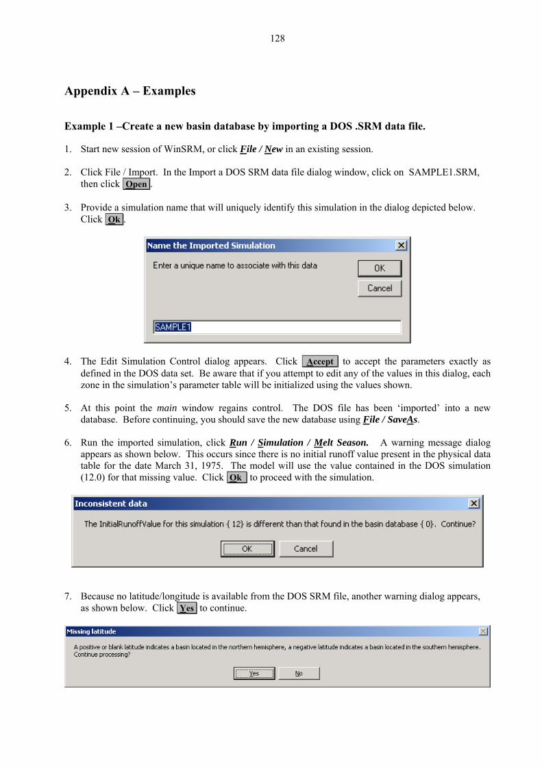
128

Ap

Exa

1.

pendix A – Examples

mple 1 –Create a new basin database by importing a DOS .SRM data file.

Start new session of WinSRM, or click File / New in an existing session.

Click File / Import. In the Import a DOS SRM data file dia2. log window, click on SAMPLE1.SRM, then click Open .

3. og depicted below. Provide a simulation name that will uniquely identify this simulation in the dial

Click Ok .

4. The Edit Simulation Control dialog appears. Click Accept to accept the parameters exactly as

defined in the DOS data set. Be aware that if you attempt to edit any of the values in this dialog, each zone in the simulation’s parameter table will be initialized using the values shown.

5. At this point the main window regains control. The DOS file has been ‘imported’ into a new

database. Before continuing, you should save the new database using File / SaveAs. 6. un the imported simulation, click R Run / Simulation / Melt Season. A warning message dialog

pears as shown below. This occurs since there is no initial runoff value present in the physical data ble for the date March 31, 1975. The model will use the value contained in the DOS simulation

apta(12.0) for that missing value. Click Ok to proceed with the simulation.

7. Because no latitude/longitude is available from the DOS SRM file, another warning dialog appears, as shown below. Click Yes to continue.

129

8. U letion of the simulation, the Results dialog appears, as shown below. After examining the pon compstatistics, click Done to return to the main window.

9. Ap

fter the successful simulation, you can familiarize yourself with the graphical and tabular output roducts available to the modeler by clicking Graphics or Reports on the main menu.

1. L

Example 2 - Adding physical data to a database from another (digital) source

oad the database created in Example 1, or any of the other sample WinSRM databases.

2. Click Add Simulation , enter a new simulation in the Name the New Simulation dialog, then click Ok . The Edit Simulation Control Information window appears.

3. For purposes of this example, the default information in this dialog will be used as presented. Click

Accept to add the new simulation to the database. Two dialogs appear as shown below:

Click Ok .

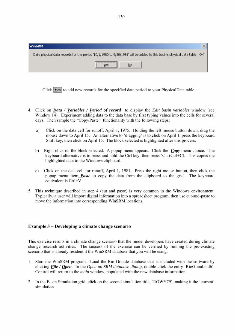
130

Click Yes to add new records for the specified date period to your PhysicalData table.

4. Click on Data / Variables / Period of record to display the Edit basin variables window (see

Window 14). Experiment adding data to the data base by first typing values into the cells for sevdays. Then sample the “Copy/Paste” functionality with the following steps:

a) Click on the data cell for runoff, April 1,

eral

1975. Holding the left mouse button down, drag the lternative to ‘dragging’ is to click on April 1, press the keyboard

s. Click the C

mouse down to April 15. An aShift key, then click on April 15. The block selected is highlighted after this process.

opy menu choice. The

e

b) Right-click on the block selected. A popup menu appearkeyboard alternative is to press and hold the Ctrl key, then press ‘C’. (Ctrl+C). This copies the highlighted data to the Windows clipboard.

c) Click on the data cell for runoff, April 1, 1981. Press the right mouse button, then click th

popup menu item Paste to copy the data from the clipboard to the grid. The keyboard equivalent is Ctrl+V.

5. This technique described in step 4 (cut and paste) is very common in the Windows environment.

Typically, a user will import digital

information into a spreadsheet program, then use cut-and-paste to locations.

g climate running the pre-existing

that you will be using.

e database that is included with the software by

move the information into corresponding WinSRM

Example 3 – Developing a climate change scenario

opers have created durinThis exercise results in a climate change scenario that the model devel

ise can be verified bychange research activities. The success of the exercdatabasescenario that is already resident it the WinSRM

1. Start the WinSRM program. Load the Rio Grand

clicking File / Open. In the Open an SRM database dialog, double-click the entry ‘RioGrand.mdb’. ase information.

, click on the second simulation title, ‘RGWY79’, making it the ‘current’

Control will return to the main window, populated with the new datab 2. In the Basin Simulation grid

simulation.

131

3. Click on Data / Climate Change Scenario Definition. The Climate Change Scenario Definition for Simulation: RGWY79 window appears (See Window 16). Click New . The Create a new climate change scenario dialog appears. Enter the name Ex3 for your new climate change scenario.

4. The definition dialog is initialized to an empty, new state. Notice the simulation period cannot b

changed, and that it is one year in lenge

th. WinSRM performs climate change over a one-year period only. Notice also that the Winter End Date defaults to the halfway point in the year. This value may

5. that

temperature will be warmer by 4oC throughout the entire year in your changed climate.

a) b) the simulation

starting date. Double-click the ending date cell to set the change’s ending date to the simulation ending date.

c) Click on the Edit Action drop-down list and select Add to each day. Type 4 into the Edit Factor cell.

d) Select All from the Zone drop-down list, meaning this rule will apply to temperatures in every zone.

e) In Row 2, select Degree-Day Factor from the Variable/Parameter drop-down. f) Set the date period in row 2 by repeating step (b). g) Select Shift Backward from the Edit Action drop-down. (the increased temperature of the

changed-climate necessitates utilization of the warmer month’s DD factors earlier in the season than would occur in the present climate).

h) Enter 31 as the edit factor for this rule line. When used with ‘shifts’, the edit factor is the number of days to shift the parameter (e.g., a shift backward of 15 days moves 4/16 to 4/1, 4/17 to 4/2, etc.).

i) For Row 3, select Snow Runoff Coefficients from the Variable/Parameter drop-down. Complete the line by repeating steps (f), (g), and (h).

6. Click Done to close the Climate Change Scenario Definition dialog and return control to the main

window. To preserve the newly created scenario, click F

be modified by the user.

Begin creating your set of ‘rules’ that will define your changed climate. You estimate

In Row 1, click the Variable/Parameter drop-down list and select Average Temperature. Double-click the starting date cell to set the starting date for this change to

ile / Save.

Example 4 – Simulating climate change using a climate change scenario

This exercise uses the climate change scenario, Ex3, developed in the previous example. If Example 3 was skipped, the climate change scenario Tplus4 can be substituted for Ex3. Skip steps 1 and 2 if you have proceeded to this example directly from completion of Example 3. 1. Start the software by

clicking F WinSRM program. Load the Rio Grande database that is included with the

ile / Open. In the Open an SRM database dialog, double-click the entry ‘RioGrand.mdb’. C

2. C tions grid, making it the current simulation. . C

ontrol will return to the main window, populated with the new database information. lick on ‘RGWY79’ in the Basin Simulalick 3 Run / Climate Change to begin the climate change simulation process. The Run a Climate

e RGWY79.

Change window appears. 4. Select Ex3 from the Scenario Definition(s) for RGWY79 drop-down list. This list contains all th

scenarios in the database that have been created to use with simulation 5. Click Step1: Winter, Present Climate to begin the climate change simulation. As with any normal

simulation, the model first initializes the SimResults table with a copy of variables and parameters taken from the database that are required to drive the simulation. Next, using the rules contained in

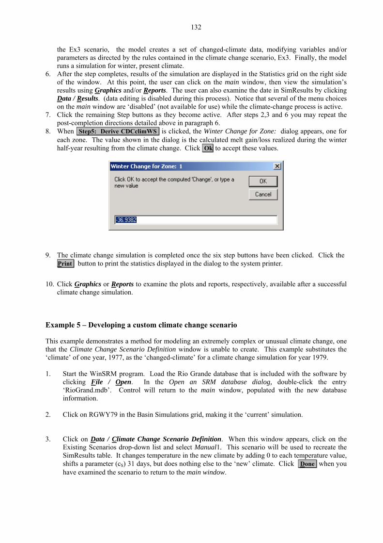
132

the Ex3 scenario, the model creates a set of changed-climate data, modifying variables and/orparameters as directed by the rules contained

in the climate change scenario, Ex3. Finally, the model

runs a simulation for winter, present climate. 6 After the step completes, results of the simulation are displayed in the Statistics grid on the right side

of the windo the simulation’s results using G

. w. At this point, the user can click on the main window, then view

raphics and/or Reports. The user can also examine the date in SimResults by clicking Data / Results. (data editing is disabled during this process). Notice that several of the menu choices

ve. 7. aining Step buttons as they become active. After steps 2,3 and 6 you may repeat the

on the main window are ‘disabled’ (not available for use) while the climate-change process is actiClick the rempost-completion directions detailed above in paragraph 6.

8. pears, one for When Step5: Derive CDCclimWS is clicked, the Winter Change for Zone: dialog apeach zone. The value shown in the dialog is the calculated melt gain/loss realized during the winter half-year resulting from the climate change. Click Ok to accept these values.

9. The climate change simulation is completed once the six step buttons have been clicked. Click the Print button to print the statistics displayed in the dialog to the system printer.

10. Click Graphics or Reports to examine the plots and reports, respectively, available after a successful

climate change simulation.

by

Example 5 – Developing a custom climate change scenario

This example demonstrates a method for modeling an extremely complex or unusual climate change, onethat the Climate Change Scenario Definition window is unable to create. This example substitutes the‘climate’ of one year, 1977, as the ‘changed-climate’ for a climate change simulation for year 1979. 1. Start the WinSRM program. Load the Rio Grande database that is included with the software

clicking File / Open. In the Open an SRM database dialog, double-click the e‘RioGrand.mdb’. Control will return

ntry to the main window, populated with the new database

information. 2. Click on RGWY79 in the Basin Simulations grid, making it the ‘current’ simulation. 3. Click on Data / Climate Change Scenario Definition. When this window appears, click on the

Existing Scenarios drop-down list and select Manual1. This scenario will be used to recreate the SimResults table. It changes temperature in the new climate by adding 0 to each temperature value, shifts a parameter (cS) 31 days, but does nothing else to the ‘new’ climate. Click Done when you have examined the scenario to return to the main window.

133

4. Click on Run / Climate Change. The Run a Climate Change window appears. Select Manual1 from the Scenario Definition(s) … drop-down list. Click on Step1: Winter, Present Climate . As explained above (Example 4, Step 5) the model recreates the SimResults table using the selected scenario to generate the ‘changed’ climate variables and/or parameters. In the example, the only effective change is the 31-day shift of snow runoff coefficients (cS). Simulation.

5. After Step1 completes, click on Abort to terminate the simulation. Control returns to the main

window. Now we will begin to ‘customize’ the SimResults table with a changed-climate that would be impossible to accomplish with a climate change scenario, by cutting-and-pasting the climate variables (temperature and precipitation) from 1977 to 1979’s new climate. 6. Click on RGWY77 in the Basin Simulations grid. Click on Data / Variables / Current Simulation.

The Edit basin variables dialog appears. Click on the column header Tavg. The entire column should be ‘highlighted’. Right-click on this column, then select Copy (or press Ctrl+C) to copy the year of temperature data for zone A to the Windows clipboard. Click Cancel to close the dialog and return to the main window.

7. Click on RGWY79 in the Basin Simulations grid. Click on Data / Results. The Simulation results

ting dialog appears. Notice that a number of the column headers end with ‘CC’. These cedi olumns contain the post-climate-change values for that variable/parameter. If a column header is only partially visible you can resize the column by placing the mouse on a column border in the header. When the mouse changes state, press the left mouse button and drag to complete the resize.

8. Click on the column header TavgCC to select the entire column. The column will be highlighted.

Right-click the column and select Paste from the popup menu (or press Ctrl+V). The data copied to the clipboard in Step 6 will replace the data in the column. Since the temperature distribution for RGWY79 is ‘Basinwide’ (see the main window), no further temperature modification is necessary. (Basinwide variables are always stored in Zone 1 in WinSRM tables). Click Done to close the dialog and return to the main window.

9. Click on RGWY77 in the Basin Simulations grid. Click on Data / Variables / Current Simulation.

The Edit basin variables dialog appears. Click on the column header Precip. The entire column should be ‘highlighted’. Right-click on this column, then select Copy (or press Ctrl+C) to copy the precipitation data for zone A to the clipboard. Click Cancel to close the dialog and return to the main window.

10. Click on RGWY79 in the Basin Simulations grid. Click on Data / Results. The Simulation results

editing dialog appears. Click on the column header PrecipCC. The entire column should be ‘highlighted’. Right-click the column and select Paste from the popup menu (or press Ctrl+V). The 1977 precipitation data copied to the clipboard in Step 9 will replace the data in the column. Click Done to close the dialog and return to the main window.

11. Copy the 1977 precipitation for zones B and C to SimResults zones B and C by repeating steps

9&10 for each zone. 12. At this point your customized climate change definition is complete. Before running the climate

change simulation you may want to save the database to preserve the SimResults table in its customized form (there is only one SimResults table per database. The table is recreated each time a simulation is performed).

134

13. Click Run / Climate Change. The Run a Climate Change window appears. Select Manual1 from -down list. (the model uses the winter-end-date found in this

4. Click the Use the climate changes defined in Results checkbox .

the Scenario Definitions(s)… dropscenario).

1 15. Click on Step1: Winter, Present Climate . Because the checkbox (Step 14) is ‘checked’, the

model skips the preliminary step that recreates the SimResults table. Instead, the table used is the one we created and edited in steps 4-10.

16. Complete the climate change simulation by following Example 4, Steps 6-10.

Example 6 – Developing a normalized year

This example illustrates the steps required to create a normalized year of temperature, precipitation and snow-depletion data, using as a source a year-round simulation selected from a WinSRM basin database. See Section 8.5

to learn more about normalized data and how it is used in simulating climate-change. See Section 10.3.8 to learn how WinSRM derives long-term monthly averages for temperature and precipitation, and how it uses these long-term averages to adjust corresponding observed daily values (during climate-change processing), resulting in a set of ‘normalized’ temperature and precipitation for the given year, and the resulting snow-depletion curve(s) derived using the ‘normalized’ climate. The example assumes that multiple years of physical data are present in the current basin database. An alternative, manual method for normalizing your data, replacing Step 4, is described at the end of this example. The alternative method demonstrates how long-term averages derived externally from other sources, are applied to the selected simulation year. 1. Load an existing WinSRM database. Click File / Open (or File followed by selecting a WinSRM database from the ‘Recent Files’ list) 2. Save the WinSRM database to a new (mirrored) database file. File/Save As After this step, the database displayed by the model screens is the new, mirror database. 3. Select a simulation from the ‘Basin Simulations’ grid. The selected simulation must be a year-round

simulation for the year you want to normalize. 4. Create a climate change scenario with temperature and/or precipitation modified using the ‘Normalize’

climate change function. Click Data/Climate Change Scenario Definition. Click New. Type in a new scenario name. Click Ok. Define a modifying rule for temperature: A. Select temperature from variable/parameter dropdown menu B. Identify the starting and ending dates (winter starting date through summer ending date) C. Select ‘Normalize’ from the edit action dropdown menu D. Type ‘0’ (zero) in the edit factor cell E. Select ‘All’ from the zone dropdown if temperature selected in sub-step A is ‘Average’ Select the ‘A’ zone if temperature option selected is Max/Min Repeat modifying rule steps above for precipitation. Change the ‘Winter End Date’ if necessary. Enter comments in the ‘Comments’ box if desired. Click Done to return to the main WinSRM window.

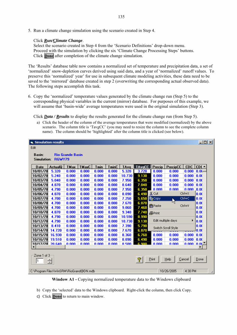
135

5. Run a climate change simulation using the s

cenario created in Step 4.

Click Run/Climate Change. Select the scenario created in Step 4 from the ‘Scenario Definitions’ drop-down menu. Proceed with the simulation by clicking the six ‘Climate Change Processing Steps’ buttons. Click Done after completion of the climate change simulation. The ‘Results’ database table now contains a normalized set of temperature and precipitation data, a set of ‘normalized’ snow-depletion curves derived using said data, and a year of ‘normalized’ runoff values. To preserve this ‘normalized’ year’ for use in subsequent climate modeling activities, these data need to be saved to the ‘mirrored’ database created in step 2 (overwriting the corresponding actual observed data). The following steps accomplish this task. 6. Copy the ‘normalized’ temperature values generated by the climate change run (Step 5) to the

corresponding physical variables in the current (mirror) database. For purposes of this example, we will a that ‘basin-wide’ average temperatssume ures were used in the original simulation (Step 3).

Click Data / Res to he lts generated for the climate change run (from Step 5). ults display t resu

a) Click the header of the column of the average temperatures that were modified (normalized) by the above scenario. The column title is ‘TavgCC’ (you may need to resize the column to see the complete column name). The column should be ‘highlighted’ after the column title is clicked (see below).

Window A1 - Copying normalized temperature data to the Windows clipboard

b) Copy the ‘selected’ data to the Windows clipboard. Right-click the column, then click Copy. c) Click Done to return to main window.

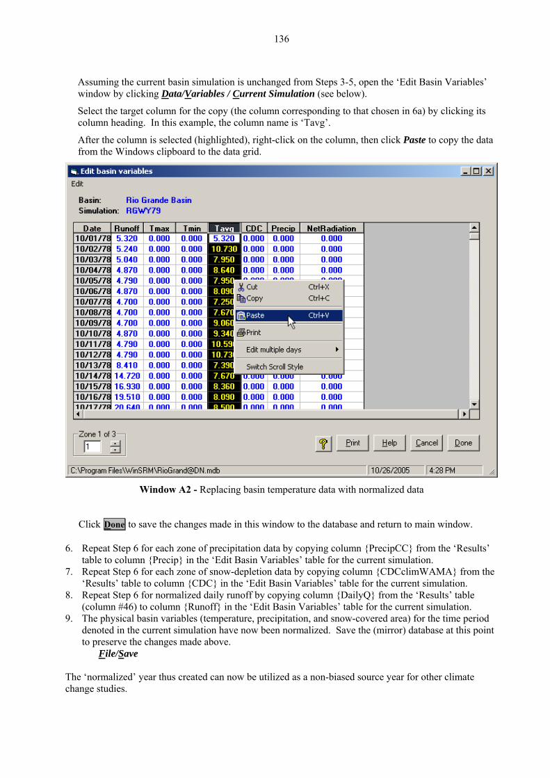
136

Assuming the current basin simulation is unchanged from Steps 3-5, open the ‘Edit Basin Variables’

window by clicking Data/Variables / Current Simulation (see below).

After the column is selected (highlighted), right-click on the column, then click Paste to copy the data ard to the data grid.

Select the target column for the copy (the column corresponding to that chosen in 6a) by clicking its column heading. In this example, the column name is ‘Tavg’.

from the Windows clipbo

Window A2 - Replacing basin temperature data with normalized data

Click Done to save the chan in se and return to main window. ges made this window to the databa

tep 6 for each zone ipita the ‘Results’ cip} in t Ba

the ’ table to column {C the rent simulation.

for normalize runon {Runoff} in the ‘Edit Basi

in varia es (temperature, precipitation, and snow-covered area) for the time period denoted in the current simulation have now been normalized. Save the (mirror) database at this point to preserve the changes made above.

F

6. Repeat S of prec tion data by copying column {PrecipCC} fromtable to column {Pre

7. Repeat Step 6 for each zone of snow-depleti the ‘Edi sin Variables’ table for the current simulation.

on data by copying column {CDCclimWAMA} from‘Results DC} in ‘Edit Basin Variables’ table for the cur

8. Repeat Step 6(column #46) to colum

d daily ff by copying column {DailyQ} from the ‘Results’ table n Variables’ table for the current simulation.

9. The physical bas bl

ile/Save The ‘normalized’ year thus created can now be utilized as a non-biased source year for other climate change studies.

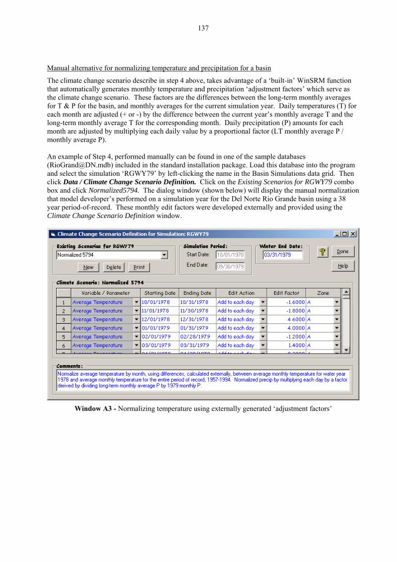
137

Manual alternative for normalizing temperature and precipitation for a basin

mperatures (T) for ach month are adjusted (+ or -) by the difference between the current year’s monthly average T and the ng-term monthly average T for the corresponding month. Daily precipitation (P) amounts for each

month ultiplying each daily value by a proportional thly average P / monthly average P).

of Step 4, performe aldb) included in the standard installati lation ‘RGWY79’ by l in Simulations data grid. Then

mate Change Sc D bo Normalized5794. eloper’s performe sim 8

-of-record. These m Climate Change Scenario Definition window.

The climate change scenario describe in step 4 above, takes advantage of a ‘built-in’ WinSRM function that automatically generates monthly temperature and precipitation ‘adjustment factors’ which serve as the climate change scenario. These factors are the differences between the long-term monthly averages for T & P for the basin, and monthly averages for the current simulation year. Daily teelo

are adjusted by m factor (LT mon

An example d manu ly can be found in one of the sample databases ([email protected] select the simu

on package. Load this database into the programeft-clicking the name in the Bas

click Data / Cli enario efinition. Click on the Existing Scenarios for RGWY79 combox and click that model dev

The dialog window (shown below) will displayd on a

the manual normalization ulation year for the Del Norte Rio Grande basin using a 3

year period onthly edit factors were developed externally and provided using the

Window A3 - Normalizing temperature using externally generated ‘adjustment factors’

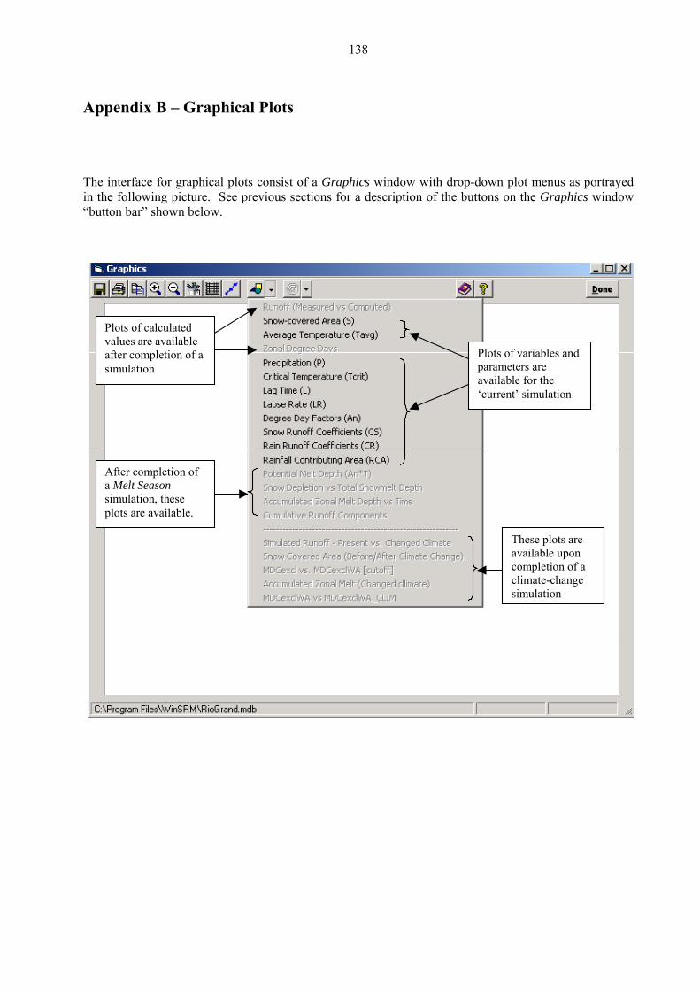
138

Appendix B – Graphical Plots

The interface for graphical plots consist of a Graphics window with drop-down plot menus as portrayed in the following picture. See previous sections for a description of the buttons on the Graphics window “button bar” shown below.

Plots of variables andparameters areavailable for the‘current’ simulation.

Plots of calculatedvalues are available

completion simulationafter of a

After completion ofa Melt Seasonsimulation, these

s are availabplot le.

These plots areavailable uponcompletion of aclimate-changesimulation

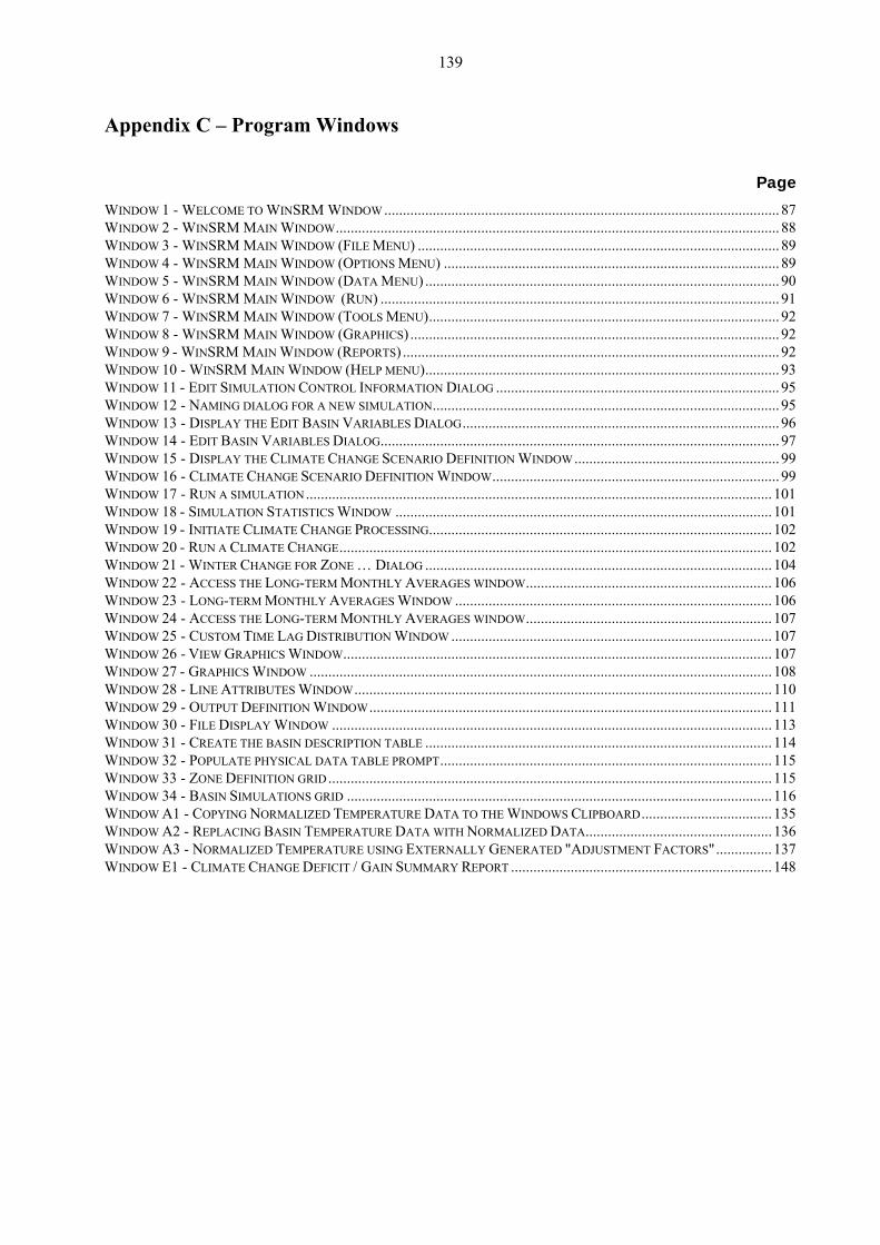
139

Appendix C – Program Windows

Page

WINDOW 1 - WELCOME TO WINSRM WINDOW .......................................................................................................... 87 W SR WINDOW....................................................................................................................... 88

SR WINDOW (FILE MENU) ................................................................................................. 89 WINDOW 4 - WINSRM M WINDOW (OPTIONS MENU) .......................................................................................... 89

W 5 - WINSR ..................................................................................... 90 6 - WINSRM M WINDOW 91

W 7 - WINSRM W ........... 92 WINDOW 8 - WINSRM MAIN WINDOW WINDOW 9 - WINSRM MAIN W

W 10 - WINS WWINDOW 11 - EDIT SIMULATION WINDOW 12 - NAMING DIALOG FOR WINDOW 13 - DISPLAY THE EDIT

- EDIT B RIA - DISPL LIM

WINDOW 16 - CLIMATE CHANGE EFINITION WINDOW............................................................................. 99 WINDOW 17 - RUN A SIMULATION 101 WINDOW 18 - SIMULATION STAT WINDOW 19 - INITIATE CLIMATE

RUN A C WINDOW 21 - WINTER CHANGE IALOG ............................................................................................. 104 WINDOW 22 - ACCESS THE LONGWINDOW 23 - LONG-TERM MONTH WINDOW 24 - ACCESS THE LONG 07

DOW 25 - CUSTO AWINDOW 26 - VIEW GRAPHICS W ........................................................................... 107 WINDOW 27 - GRAPHICS WINDOWINDOW 28 - LINE ATTRIBUTES

DOW 29 - OUTPUWINDOW 30 - FILE DISPLAY WINWINDOW 31 - CREATE THE BASIN ON TABLE ............................................................................................. 114 WINDOW 32 - POPULATE PHYSICAL DATA TABLE PROMPT......................................................................................... 115 WINDOW 33 - ZONE DEFINITION

DOW 34 - BASIN IODOW A1 - COPYI A

WINDOW A2 - REPLACING BASIN RE DATA WITH NORMALIZED DATA.................................................. 136 WINDOW A3 - NORMALIZED TEMPERATURE USING EXTERNALLY GENERATED "ADJUSTMENT FACTORS"............... 137 WINDOW E1 - CLIMATE CHANGE

INDOW 2 - WINWINDOW 3 - WIN

M MAIN M MAIN

AIN WINDO M MAIN WINDOW (DATA MENU) ..........WINDOW WINDO

AIN MAIN

(RUN) ...........................................................................................................INDOW (TOOLS MENU)...................................................................................

(GRAPHICS) ................................................................................................... 92INDOW (REPORTS) ..................................................................................................... 92

INDOW (HELP MENU)............................................................................................... 93 CONTROL INFORMATION DIALOG ............................................................................ 95

WINDO RM MAIN

A NEW SIMULATION............................................................................................. 95 BASIN VARIABLES DIALOG..................................................................................... 96 BLES DIALOG........................................................................................................... 97 ATE CHANGE SCENARIO DEFINITION WINDOW....................................................... 99

SCENARIO D

WINDOW 14WINDOW 15

ASIN VAAY THE C

.............................................................................................................................ISTICS WINDOW ..................................................................................................... 101 CHANGE PROCESSING............................................................................................ 102 HANGE.................................................................................................................... 102FOR ZONE … D

WINDOW 20 - CLIMATE

-TERM MONTHLY AVERAGES WINDOW.................................................................. 106 LY AVERAGES WINDOW ..................................................................................... 106

-TERM MONTHLY AVERAGES WINDOW.................................................................. 1G DISTRIBUTION WINDOW ...................................................................................... 107

INDOW........................................WIN M TIME L

W ............................................................................................................................ 108 WINDOW................................................................................................................ 110

ON WINDOW............................................................................................................ 111 DOW ...................................................................................................................... 113 DESCRIPTI

WIN T DEFINITI

GRID....................................................................................................................... 115 NS GRID .................................................................................................................. 116 LIZED TEMPERATURE DATA TO THE WINDOWS CLIPBOARD................................... 135 TEMPERATU

WINWIN

SIMULATNG NORM

DEFICIT / GAIN SUMMARY REPORT ...................................................................... 148

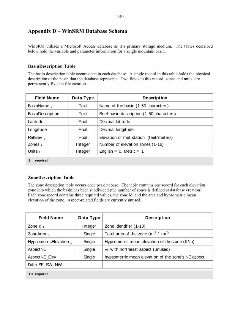
140

Appendix D – WinSRM Database Schema

eld N Data T Descr

WinSRM utilizes a Microsoft Access database as it’s primary storage medium. The tables described below hold the variable and parameter information for a single mountain basin.

BasinDescription Table The basin description table occurs once in each database. A single record in this table holds the physical description of the basin that the database represents. Two fields in this record, zones and units, are permanently fixed at file creation.

Fi ame ype iption

Bas Na Text me o aracters) in me 1 Na f the basin (1-50 ch

BasinDescription Text rief ba ters) B sin description (1-50 charac

Lat de Float cimalitu De latitude

Lon tu Float cimalgi de De longitude

Re ev 1 Float evatiofEl El n of met station (feet/meters)

Zones 1 Integer mber (1-16) Nu of elevation zones

Units 1 Integer glish En = 0, Metric = 1

Zo n Table Th n cription table occurs on databa ins one record for each elevation zone into which the basin has been subdivided (the number of zones is defined at database creation). Each zone record contains three required values, the zone id, and the area and hypsometric mean elevation of the zone. Aspect-related fields are currently unused.

Data T Description

1 = required

neDescriptioe zo e des ce per se. The table conta

Field Name ype

ZoneId 1 Integer Zone identifier (1-10)

ZoneArea 1 Single Total area of the zone (mi2 / km2)

HypsometricElevation 1 Single Hypsometric mean elevation of the zone (ft/m)

AspectNE Single % with northeast aspect (unused)

AspectNE_Elev Single hypsometric mean elevation of the zone's NE aspect

Ditto SE, SW, NW 1 = u req ired

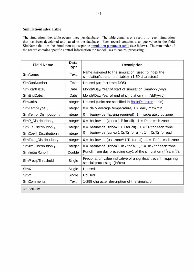
141

SimulationIndex Table The sim dex table occurs o datab e record for each simulation that has been developed and saved value in the field Sim am ulation to a separate sim

ulationin nce per ase. The table contains onin the database. Each record contains a unique

N e that ties the sim ulation parameter table (see below). The remainder of the o tains specific control ion th

Field Name DatTyp Description

rec rd con informat e model uses to control processing.

a e

Sim m Te ame axt Nsimulation’s parameter table) (1-50 characters)

ssigned to the simulation (used to index the Na e1

SimRunNumber Text Unused (artifact from DOS)

SimStartDate Date Month/Day/Year of start of simulation (mm/dd/yyyy) 1

SimEndDate1 Date Month/Day/Year of end of simulation (mm/dd/yyyy)

SimUnits Integer nusedU (units are specified in BasinDefiniton table)

SimTempType 1 Integer 0 = daily average temperature, 1 = daily max/min

SimTemp_Distribution 1 Integ = ba nwide (lapsing required), 1 = separately by zone er 0 si

SimP_Distribution 1 Integ = ba nwide (zone#1 P for all) , 1 = P for each zone er 0 si

SimLR_Distribution 1 Integ = ba nwide (zone#1 LR for all) , 1 = LR for each zone er 0 si

SimCoeff_Distribution 1 Integ = ba nwide (zone#1 Cs/Cr for all) , 1 = Cs/Cr for each er 0 sizone

SimTcrit_Distribution 1 Integ = ba nwide (use zone#1 Tc for all) , 1 = Tc for each zone er 0 si

SimXY_Distribution 1 Integ = ba nwide (zone#1 X/Y for all) , 1 = X/Y for each zone er 0 si

SimInitialRunoff Double unoff om day preceding day1 of the simulation (f 3/s, m3/s R fr)

SimPrecipThreshold Single recipit tion value indicative of a significant event, requiring pecial rocessing. (in/cm)

P as p

SimX Single nusedU

SimY Single nusedU

SimComments Text -255 character description of the simulation 1

1 = u req ired

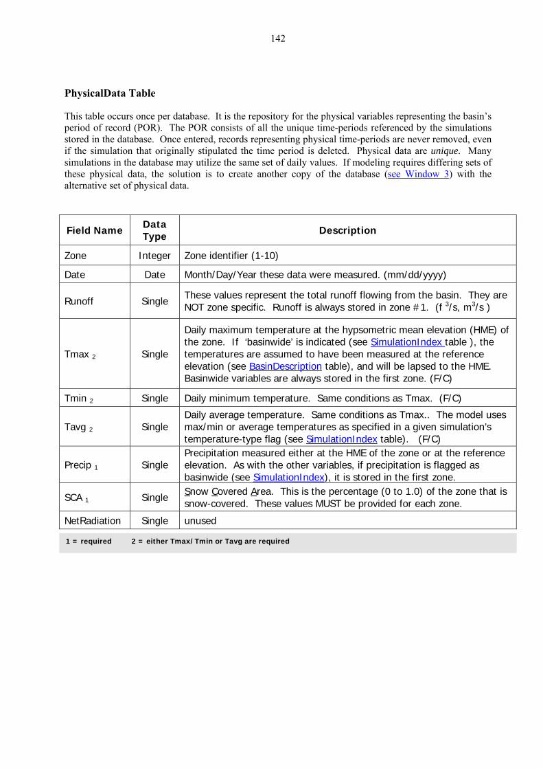
142

PhysicalData Table

This table occurs once per database. It is the repository for the physical variables representing the basin’s s n y

atabase may utilize the same set of daily values. If modeling requires differing sets of ese physical data, the solution is to create another copy of the database (see Window 3

period of record (POR). The POR consists of all the unique time-periods referenced by the simulationstored in the database. Once entered, records representing physical time-periods are never removed, eveif the simulation that originally stipulated the time period is deleted. Physical data are unique. Mansimulations in the dth ) with the alternative set of physical data.

Fi N

ame DataType Description eld

Zo ger Zone i ier (1-ne Inte dentif 10)

Date Date Month/Day/Year these data were measured. (mm/dd/yyyy)

Runoff Single These values represent the total runoff flowing from the basin. They are NOT zone specific. Runoff is always stored in zone #1. (f 3/s, m3/s )

Tmax 2 Single

Daily maximum temperature at the hypsometric mean elevation (HME) of the zo ‘basi dex nwide’ is indicated (see SimulationInne. If table ), the temperatures are assumed to have been measured at the reference elevation (see BasinDescription table), and will be lapsed to the HME. Basinwide variables are always stored in the first zone. (F/C)

Tmin 2 Single Daily minimum temperature. Same conditions as Tmax. (F/C)

Tavg 2 Single Daily average temperature. Same conditions as Tmax.. The model uses max/min or average temperatures as specified in a given simulation’s temperature-type flag (see SimulationIndex table). (F/C)

Precip 1 Single Precipitation measured either at the HME of the zone or at the reference elevation. As with the other variables, if precipitation is flagged as basinwide (see SimulationIndex), it is stored in the first zone.

SCA 1 Single Snow Covered Area. This is the percentage (0 to 1.0) of the zone that is snow-covered. These values MUST be provided for each zone.

NetRadiation Single unused

1 = required 2 = either Tmax/Tmin or Tavg are required

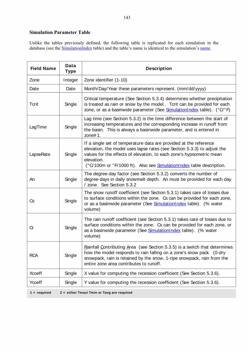
143

Simulation Parameter Table

Unlike the tables previously defined, the following table is replicated for each simulation in the database (see the SimulationIndex table) and the table’s name is identical to the simulation’s name.

Field Name Data Type Description

Zone r Zone identifier (1-10) Intege

Date Date M y/onth/Da Year these parameters represent. (mm/dd/yyyy)

Tcrit Single Cri mp precipitation is treated as rain or snow by the model.. Tcrit can be provided for each zon as

tical te erature (See Section 5.3.4) determines whether

e, or a basinwide parameter (See SimulationIndex table). (°C/°F)

La im Single

Lag time (see Section 5.3.2) is the time difference between the start of increasing temperatures and the corresponding increase in runoff from the basin. This is always a basinwide parameter, and is entered in zo

gT e

ne#1.

LapseRate

If a single set of temperature data are provided at the reference elevation, the model uses lapse rates (see Section 5.3.3) to adjust the

for the ffect of elevation, to each zone’s hypsometric mean elevation. (°C/100m or °F/1000 ft). Also see SimulationIndex

Single values e s

table description.

An Single The degree-day factor (see Section 5.3.2) converts the number of degree-days in daily snowmelt depth. An must be provided for each day / zone. See Section 5.3.2

Cs Single

The snow runoff coefficient (see Section 5.3.1) takes care of losses due to surface conditions within the zone. Cs can be provided for each zone, or as a basinwide parameter (See SimulationIndex table). (% water volume)

Cr Single

The rain runoff coefficient (see Section 5.3.1) takes care of losses due to surface conditions within the zone. Cs can be provided for each zone, or as a basinwide parameter (See SimulationIndex table). (% water volume)

RCA Single

Rainfall Contributing Area (see Section 5.3.5) is a switch that determines how the model responds to rain falling on a zone’s snow pack. (0-dry snowpack, rain is retained by the snow, 1-ripe snowpack, rain from the

zone a a c tri tes to runoff. entire re on bu

Xcoeff Single X value for computing the recession coefficient (See Section 5.3.6).

Ycoeff Single Y value for computing the recession coefficient (See Section 5.3.6).

1 = required 2 = either Tmax/Tmin or Tavg are required

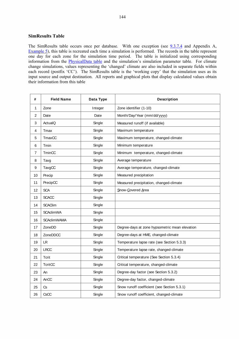
144

SimResults Table

The SimResults table occurs once per database. With one exception (see 9.3.7.4 and Appendix A, Example 5), this table is recreated each time a simulation is performed. The records in the table represent one day for each zone for the simulation time period. The table is initialized using corresponding information from the PhysicalData table and the simulation’s simulation parameter table. For climate change simulations, values representing the ‘changed’ climate are also included in separate fields within each record (postfix ‘CC’). The SimResults table is the ‘working copy’ that the simulation uses as its input source and output destination. All reports and graphical plots that display calculated values obtain their information from this table

# Field Name Data Type Description

1 Zone Integer Zone identifier (1-10)

2 Date Date Month/Day/Year (mm/dd/yyyy)

3 ActualQ Single Measured runoff (if available)

4 Tmax Single Maximum temperature

5 TmaxCC Single Maximum temperature, changed-climate

6 Tmin Single Minimum temperature

7 TminCC Single Minimum temperature, changed-climate

8 Tavg Single Average temperature

9 TavgCC Single Average temperature, changed-climate

10 Precip Single Measured precipitation

11 PrecipCC Single Measured precipitation, changed-climate

12 SCA Single Sn Cow- overed Area

13 SCACC Single

14 SCAClim Single

15 SCAclimWA Single

16 SCAclimWAMA Single

17 ZoneDD Single Degree-days at zone hypsometric mean elevation

18 ZoneDDCC Single Degree-days at HME, changed-climate

19 LR Single Temperature lapse rate (see Section 5.3.3)

20 LRCC Single Temperature lapse rate, changed-climate

21 Tcrit Single Critical temperature (See Section 5.3.4)

22 TcritCC Single Critical temperature, changed-climate

23 An Single Degree-day factor (see Section 5.3.2)

24 AnCC Single Degree-day factor, changed-climate

25 Cs Single Snow runoff coefficient (see Section 5.3.1)

26 CsCC Single Snow runoff coefficient, changed-climate

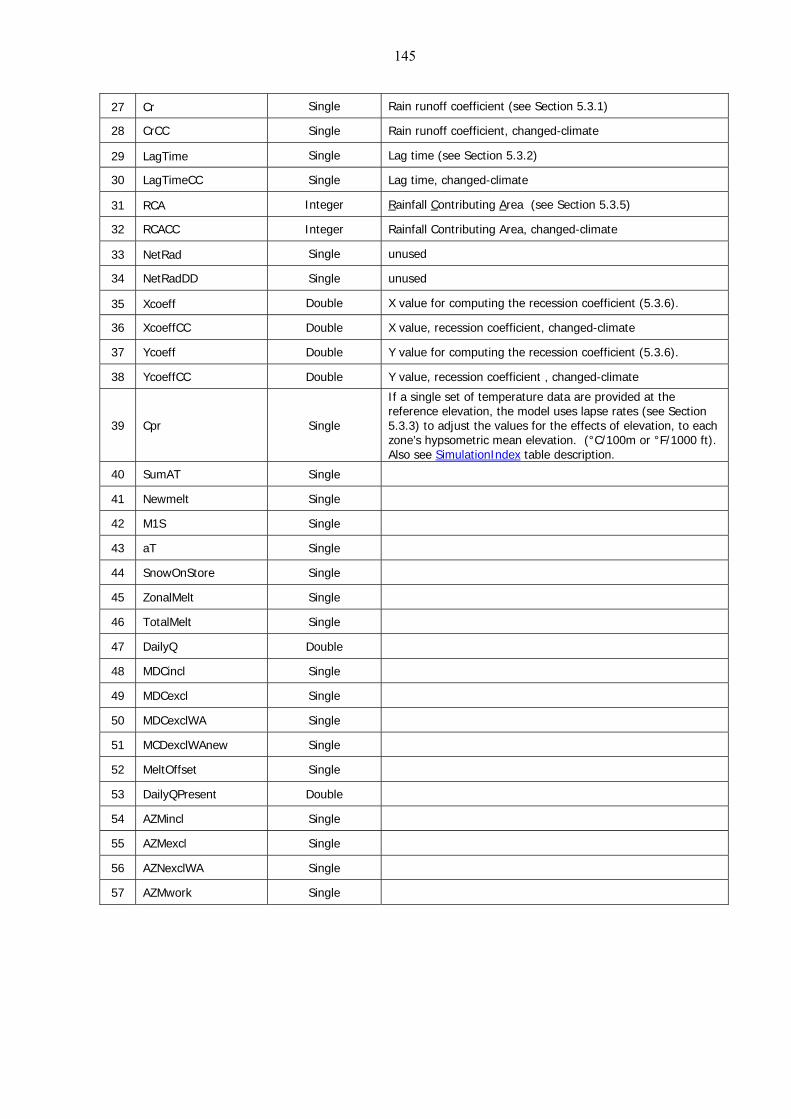
145

27 Cr Single Rain runoff coefficient (see Section 5.3.1)

28 CrCC Single Rain runoff coefficient, changed-climate

29 LagTime Single Lag time (see Section 5.3.2)

30 LagTimeCC Single Lag time, changed-climate

31 RCA Integer Rainfall Contributing Area (see Section 5.3.5)

32 RCACC Integer Rainfall Contributing Area, changed-climate

33 NetRad Single unused

34 NetRadDD Single unused

35 Xcoeff Double X value for computing the recession coefficient (5.3.6).

36 XcoeffCC Double X value, recession coefficient, changed-climate

37 Ycoeff Double Y value for computing the recession coefficient (5.3.6).

38 YcoeffCC Double Y value, recession coefficient , changed-climate

39 Cpr Single reference elevation, the model uses lapse rates (see Section 5.3.3) to ad

If a single set of temperature data are provided at the

just the values for the effects of elevation, to each zone’s hypsometric mean elevation. (°C/100m or °F/1000 ft). Also see SimulationIndex table description.

40 SumAT Single

41 Newmelt Single

42 M1S Single

43 aT Single

44 SnowOnStore Single

45 ZonalMelt Single

46 TotalMelt Single

47 DailyQ Double

48 MDCincl Single

49 MDCexcl Single

50 MDCexclWA Single

51 MCDexclWAnew Single

52 MeltOffset Single

53 DailyQPresent Double

54 AZMincl Single

55 AZMexcl Single

56 AZNexclWA Single

57 AZMwork Single

146

ClimateScenarioIndex Table

ex table occurs once per database. The table contains one record for each climate scenario table present in the database. Each record in this index table also contains the name

Data Type Description

The ClimateScenarioInd

of the simulation for which the scenario table was prepared. Simulations may “own” multiple climate change scenarios.

# Field Name

1 SimulationFile Text The name of the simulation that “owns’ the scenario

2 ScenarioFile Text he scenario table that contains

the definition (rules) for the climate change scenario.

The name of t

3 WinterEndDate Date The last day of the winter half-year.

4 Crea as last changed. tionDate Date Date the scenario w

5 Comments Memo Description of the climate-change.

147

ClimateScenario Table

The C table is the mate-change scenario for a specific simula occurs , Each record

limateScenario structure that contains the clition in the database. It 1-n times within a database. Each table contains 1-n recordscontains a ‘rule’ (9.3.5.3) for temporarily altering a variable/parameter to formulate the ‘new’

climate for the simulation. See Example 3 for more information on climate scenarios.

# Field Name Data Type Description

1 VarParm Integer The number of the variable/parameter affected by the rule (see Table D-2)

2 StartDate Date The starting date of the period for which the rule applies.

3 EndDate Date The ending date of the period for which the rule applies.

4 EditAction Integer The edit action to be performed (see Table D-2)

5 EditFactor Single Value used for the edit action

5 Zones Integer The elevation zone(s) to be modified by the rule.

# Variable/parameter

0 Max/min temperature

1 Average temperature

2 Precipitation # Edit action

3 unused 0 Add edit factor to each day

4 perature 1 Multiply daily value(s) by edit factor Critical tem

5 gage forward {edit factor} number of days Lag time to 2 Shift values

6 ays Temperature lapse rate 3 Shift values backward {edit factor} number of d

7 tion only) Degree-day factor 4 Normalize values (temperature and precipita

8 Snow runoff coefficients

9 Rain runoff coefficients

10 Rainfall contributing area

Table D-2

for edit actions Numeric equivalents

11 Radiation coefficients (unused)

Table D-1 Numeric equivalents to

variables and parameters

148

Appendix E – Additional Windows

See Figure 21 andSection 8.3 (8)

See Section 8.3 (9)

Window E1 - Climate Change Deficit / Gain Summary Report

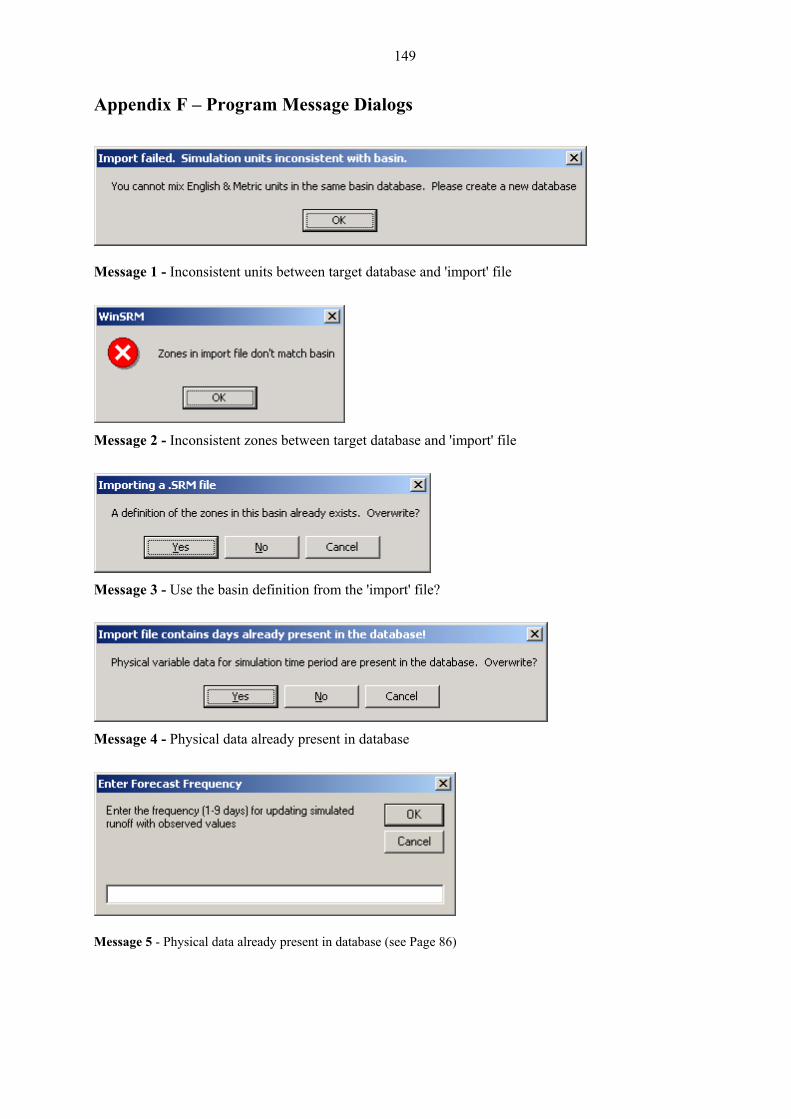
149

Appendix F – Program Message Dialogs

Message 1 - Inconsistent units between target database and 'import' file

Message 2 - Inconsistent zones between target database and 'import' file

Message 3 - Use the basin definition from the 'import' file?

Message

4 - Physical data already present in database

Message 5 - Physical data already present in database (see Page 86)

150

Appendix G – SRM Computer Program Version 4

G.1 Background

The current ve sing Microsoft QuickBASIC 4.5 and contai olbox developed by Crescent Softw G.2 Getting started

G.2.1 System

Micro-SRM re

• Any 100%

• 1 floppy ½" floppy disk. By special request, 5¼" media are available. The latest version release and documentation are also available via the Internet at:

h

rsion of the model, Micro-SRM, Version 4.0, was developed uns several subroutines from QuickPak Professional, a BASIC toare, Inc.1

requirements

quires the following persona sources: l computer re

IBM PC compatible machine

disk drive. The model is distributed on a 3

ttp://www.ars.usda.gov/Services/docs.htm?docid=8872

• A minimum of 600K availa

• A PC DOS operating system, Version 3.0 or later. SRM will run in a MS-DOS window under Microsoft Windows 3.1/95

, a graphics adapter is required. Micro-SRM supports the following graphics

soft-compatible mouse (optional).

Micro-SRM is completely contained on one distribution diskette. It may be executed directly from that diskette. The following steps describe installation on a hard disk, and assum A: are the hard disk and flopp

(1) Pu

(2) At g Enter ┘

ble random access memory (RAM)

• If graphics are desiredmodes:

- CGA - Color Graphics - EGA - Enhanced Graphics - HGA - Hercules Graphics - VGA - Virtual Graphics

• For printed output, a dot-matrix or other printer that supports a 132-character print line, either physically or using "compressed-mode" print characters

• A Micro

G.2.2 Installing Micro-SRM

e C: andy disk drives, respectively:

t ette in your floppy drive. Micro-SRM disk

the C> prompt, enter the following command lines, ending each line by pressin

1 Trademarks used in this documen S, QuickBASIC, Microsoft Corp.; QuickPak Professional, Crescent Software) are us cific information. Mention of a trade name does not constitute a guarantee or warranty for the product by the U.S. Department of Agriculture or an endorsement by the Department over other products not mentioned.

t (e.g., IBM PC, IBM CORP.; MS-DOed solely for the purpose of providing spe

151

C> cd \ : change to C: 's root directory

Th devices, printer control codes, screen dis r charac level, and video graphics mode. Included on the distribution disk are several sample ".CFG" files and a utility to cus model nfiguration.

The following list describes valid Micro-SRM command line options. Values enclosed in brackets [] denote SRM default values.

Argum

C> md \srm : create a model subdirectory

C> copy a:*.* c:\srm : copy all files from floppy A: to new subdirectory C:\SRM

G.2.3 Configuring Micro-SRM

The model uses an external "configuration" file to define the variables that Micro-SRM uses to control the interface between model and user. The configuration file is specified on the command line invoking Micro-SRM. If no filename is specified, the model uses the configuration file residing on the default directory named "SRM.CFG".

e file initializes program variables that define available diskplay colo teristics, audio tone

program, CONFIG.EXE, that gives a user the abilitytomize the 's interface for his/her unique hardware co

G.2.4 Operating instructions

The following command syntax runs Micro-SRM from the default directory. Filenames must be complete pathnames if the target file does not reside in the default directory.

SRM4 configfile {option(s)} Enter ┘

ent DescriptionConfigFile SRM.CFG]./TIN Control SRM via a trace file, not th

/TOUT tracefile e keypresses from current run in a tracefile. /TDE /TIN to vary speed of trac s

r more on the trace delay./P = p

The follo everal common command line option combinations for initiating Micro-SRM:

C > SRR ation file, C:SRM.CFG, stored in that directory.

C > A:

See description above [ = tracefile e keyboard. See previous section

for a complete description of the trace feature. = Sav

LAY = seconds Use e operation [.5]. See previou withsection fo

rintfile Redirect LPT1: (printed output) to a disk file.

wing examples demonstrate s

M4 n the model from the default (in this case the root) directory, using the default configuru

152

A > SRM4 EGA.CFG /P=SRMPRINT.PRT Switch to the A: drive, then run the model from the A: default directory. Use the A:EGA.CFG

Reroute any printed output to a disk file, A:SRMPRINT.PRT.

, run SRM using the default config file, and capture all keypresses oring then in a trace file named C:\SRM\TRACE.FL

. Drive the model with keypresses stored in C:\SRM\TRACE.FL, with a 2 second delay between commands.

configuration file. C > SRM > SRM4 /TOUT=trace.fl

From the SRM subdirectoryduring the run, st

C > C:\SRM\SRM4 C:\SRM\SRM.CFG /TIN=C:\SRM\TRACE.FL /TDELAY=2

Run SRM from the root directory, using full pathnames for all file references

C > MSHERC

SRM4 HERC.CFG Load Microsoft's Hercules graphics driver and run SRM in the Hercules graphics mode.

HINT: Create a batch file to run Micro-SRM. Store the batch file on the root directory of your hard disk and include the root directory in your PATH statement (refer to your DOS manual for a description of PATH). To create a batch (.BAT) file, type the following commands, each terminated by Enter ┘:

C> cd \ : Make root dir the current dir C> copy con SRM.BAT : Copy from keyboard to SRM.BAT cd \srm : Line #1, change to model dir srm4 : Line #2, run model cd \ :<F6>

To run M ly type the b Enter ┘

G.3 Pr

G.3.1 Sc

The mod user M through a ata and menu screens. Each screen dis

• The udes run-spec or .

• The play prompts and ng/e ges as

• The oard dicato te (on/off) of the CapsL and N boar

• The isplayed.

• Screen "hot" areas, highlighted (bold) text or characters, may appear anywhere on the screen. They draw attention to the scre they provide a region that may be "mouse-clicked", to provid ponse.

• The remaining screen area, lines 4-23, will have a type-specific definition. Micro-SRM uses three types of screen display to communicate with the model user.

Line #3, change to root dir on; : Press Function Key F6, then Enter ┘ to terminate copy c

icro-SRM using a batch file, simp atch file name, followed by

ogram features

reen display types

el interacts with Micro-SR combination of text, dplay can be broken into several component parts.

screen header, lines 1-3 of the display, identifies the screen and in some cases inclific inf mation

prom e, line 4 ns 1-71, provides a location where the program apt lin 2 , colum c n diswarni rror messa required.

keyb state" in line 24 7 displ y ent staock umLock key d keys.

" rs, , columns 4-80, a the curr

function key line, line 25, describes important functions available while the screen is d

en area, as with function keys, and e a mouse equivalent to a keypress res

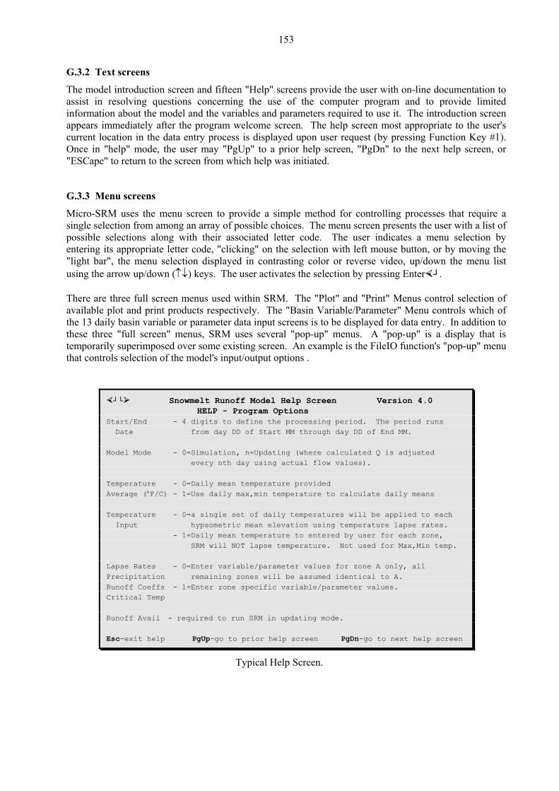
153

G.3.2 Text screens

The mod een the user with entation to assist in ns concer computer program a ovide limited informati ameters required to use it. The introduction screen appears i e user's current lo ey #1). Once in reen, or "ESCape" to return to the scr w

G.3.3 M

Micro-SR n re a single sel of st of possible as tion by entering n se ing the "light bar y list using the h p There are ection of available . The "Basin Variable/Paramthe 13 daily basin variable or param . In addition to these three "full screen" menus pop-up" is a display that is

mporarily superimposed over some existing screen. An example is the FileIO function's "pop-up" menu that controls selection of the model's input/output options .

el introd and fifteen "Help" screens provide on-line documuction scresolving questio ning the use of the nd to prr

on about the model and the variables and parmmediately after the program welcome screen. The help screen most appropriate to thcation in the data entry process is displayed upon user request (by pressing Function K

"P U Pg th t"help" mode, the user may g p" to a prior help screen, " Dn" to e nex help sceen from p inhich hel was itiated.

enu screens

M uses the menu screen to provide a simple method for co trolling processes that requi c es a liection from among an array possible hoic . The menu screen presents the user with

sel Tv

ections along with their sociated letter code. he user indicates a menu selecits appropriate letter code, "clicking" o the lection with left mouse button, or by mo", the menu selection displa ed in contrasting color or reverse video, up/down the menu

arrow up/down (↑↓) keys. T e user activates the sele ion by ressing Enter ┘. ct

three full screen menus used within SRM. The "Plot" and "Print" Menus control selplot and print products respectively eter" Menu controls which of

eter data input screens is to be displayed for data entry, SRM uses several "pop-up" menus. A "

te

┘└ Snowmelt Runoff Model Help Screen Version 4.0 HELP - Program Options Start/End - 4 digits to define the processing period. The period runs Date from day DD of Start MM through day DD of End MM. Model Mode - 0=Simulation, n=Updating (where calculated Q is adjusted every nth day using actual flow values). Temperature - 0=Daily mean temperature provided Average (°F/C) - 1=Use daily max,min temperature to calculate daily means Temperature - 0=a single set of daily temperatures will be applied to each Input hypsometric mean elevation using temperature lapse rates. - 1=Daily mean temperature to entered by user for each zone, SRM will NOT lapse temperature. Not used for Max,Min temp. Lapse Rates - 0=Enter variable/parameter values for zone A only, all Precipitation remaining zones will be assumed identical to A. Runoff Coeffs - 1=Enter zone specific variable/parameter values. Critical Temp Runoff Avail - required to run SRM in updating mode. Esc-exit help PgUp-go to prior help screen PgDn-go to next help screen

Typical Help Screen.

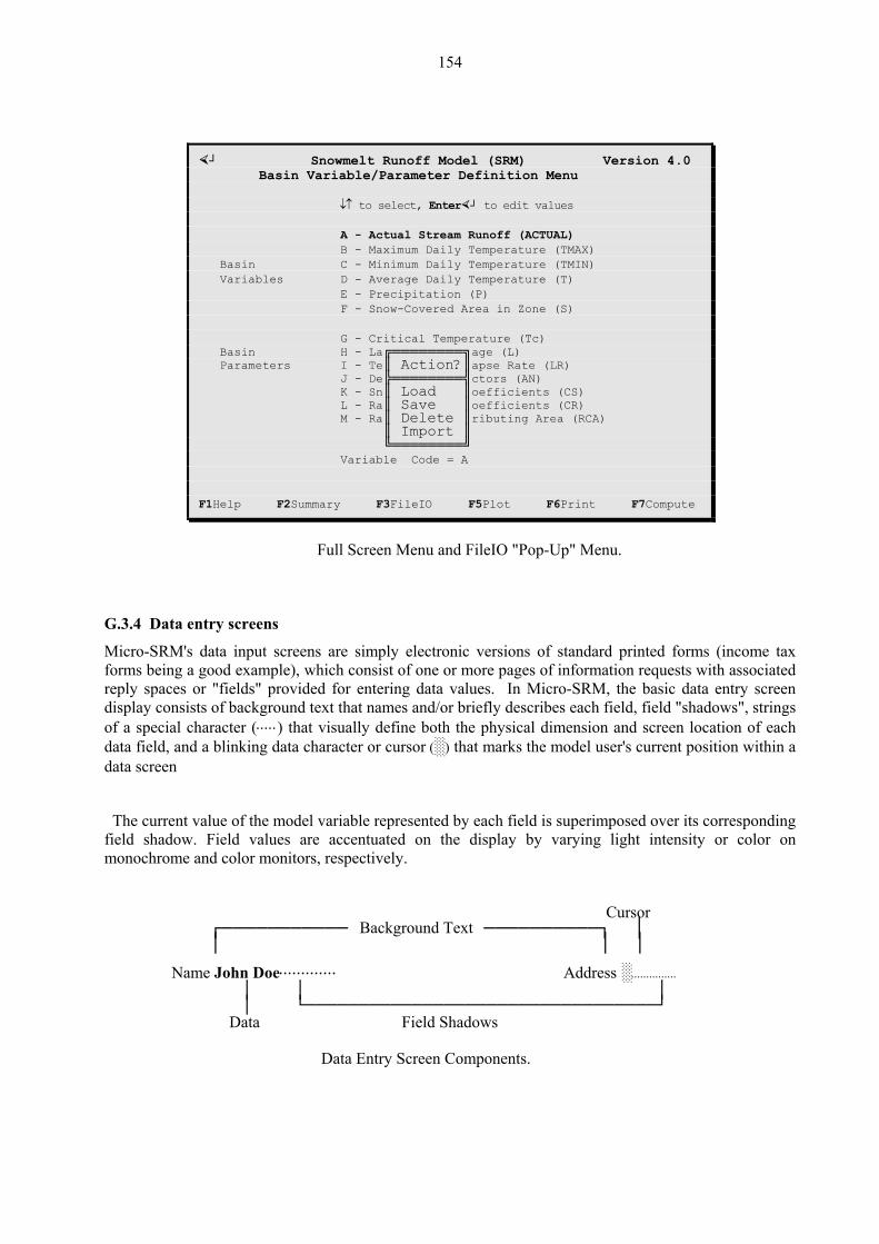
154

┘ ) Snowmelt Runoff Model (SRM Version 4.0 Basin Variable/Parameter Definition Menu

↓↑ to select, Enter ┘ to edit values A - Actual Stream Runoff (ACTUAL) B - Maximum Daily Temperature (TMAX) Basin C - Minimum Daily Temperature (TMIN) Variables D - Average Daily Temperature (T) E - Precipitation (P) F - Snow-Covered Area in Zone (S) G - Cr ical e Tc)it Temp rature ( Basin H - La ═══ ╗ag╔ ════ e (L) ═ Parameters I - Ac ║aps e R) Te║ tion? e Rat (L J - De╠════════╣ctors (AN) K - Sn║ Load ║oefficients (CS) L - Ra║ Save ║oefficients (CR) M - Ra║ Delete ║ributing Area (RCA) ║ Import ║ ╚════════╝ Variable Code = A F1Help F2Summary F3FileIO F5Plot F6Print F7Compute

Full Screen Menu and FileIO "Pop-Up" Menu.

G.3.4 Data entry screens

ach data field, and a blinking data character or cursor (░) that marks the model user's current position within a

Cursor

│ │ │ │ └─────────────────────────────────┘ Data Field Shadows

Data Entry Screen Components.

Micro-SRM's data input screens are simply electronic versions of standard printed forms (income tax forms being a good example), which consist of one or more pages of information requests with associated reply spaces or "fields" provided for entering data values. In Micro-SRM, the basic data entry screen display consists of background text that names and/or briefly describes each field, field "shadows", strings of a special character (⋅⋅⋅⋅⋅) that visually define both the physical dimension and screen location of e

data screen

The current value of the model variable represented by each field is superimposed over its corresponding field shadow. Field values are accentuated on the display by varying light intensity or color on monochrome and color monitors, respectively.

┌─────────── Background Text ──────────┐ │ │ │ │ Name John Doe⋅⋅⋅⋅⋅⋅⋅⋅⋅⋅⋅⋅⋅ Address ░⋅⋅⋅⋅⋅⋅⋅⋅⋅⋅⋅⋅⋅⋅⋅

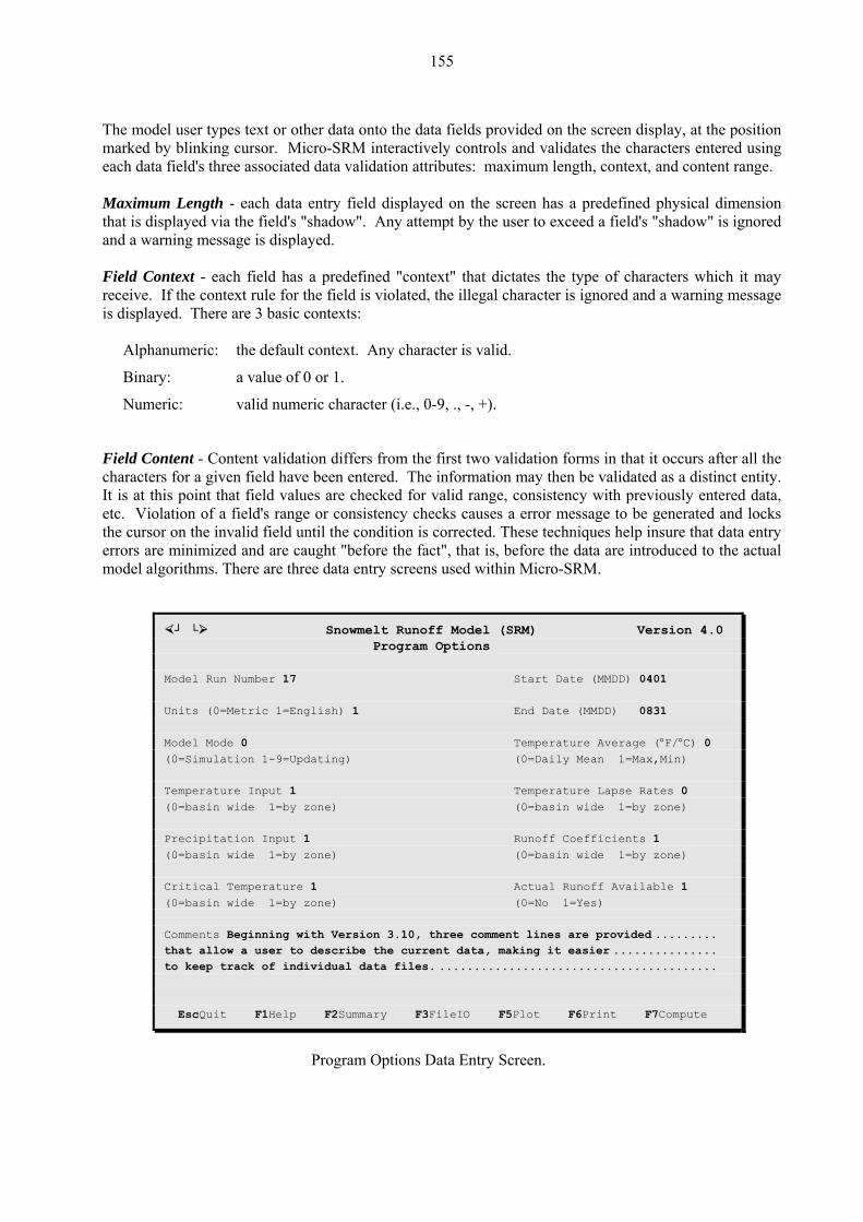
155

The model user types text or other data onto the data fields provided on the screen display, at the position marked by cursor. Micro-S using each data ciated da tent range. Maximum Length - each data entry field displayed on the screen has a predefined physical dimension that is dis " is ignored and a warnin Field Conte ters which it may receive. t t r ed and a warning message is display

Alphanum

Binary:

Nume : valid numeric character (i.e., 0-9, ., -, +).

Field Co all the character tinct entity. It is at this point that field values are checked for valid range, consistency with previously entered data, etc. Violation of a field's range rror message to be generated and locks the cursor on the invalid field un e techniques help insure that data entry errors are minimized and are caught "before the fact", that is, before the data are introduced to the actual

blinking RM interactively controls and validates the characters entered n field's three asso ta validation attributes: maximum length, context, and co

played via the field's "shadow". Any attempt by the user to exceed a field's "shadowg message is displayed.

xt - each field has a predefined "context" that dictates the type of characIf he contex ule for the field is violated, the illegal character is ignored. There are 3 basic contexts:

eric: the default context. Any character is valid.

a f 0 value o or 1.

ric

ntent - Content validation differs from the first two validation forms in that it occurs after s for a given field have been entered. The information may then be validated as a dis

or consistency checks causes a etil the condition is corrected. Thes

model algorithms. There are three data entry screens used within Micro-SRM.

┘ └ Snowmelt Runoff Model (SRM) Version 4.0 Program Options Model Run Number 17 Start Date (MMDD) 0401 Units (0=Metric 1=English) 1 End Date (MMDD) 0831 Model Mode 0 Temperature Average (°F/°C) 0 (0=Si ion 1-9=mulat Updating) (0=Daily Mean 1=Max,Min) Temperature Input 1 Temperature Lapse Rates 0 (0=basin wide 1=by zone) (0=basin wide 1=by zone) Precipitation Input 1 Runoff Coefficients 1 (0=basin wide 1=by zone) (0=basin wide 1=by zone) Critical Temperature 1 Actual Runoff Available 1 (0=basin wide 1=by zone) (0=No 1=Yes) Comments Beginning with Version 3.10, three comment lines are provided ......... that allow a user to describe the current data, making it easier ............... to keep track of individual data files. ........................................ EscQuit F1Help F2Summary F3FileIO F5Plot F6Print F7Compute

Program Options Data Entry Screen.

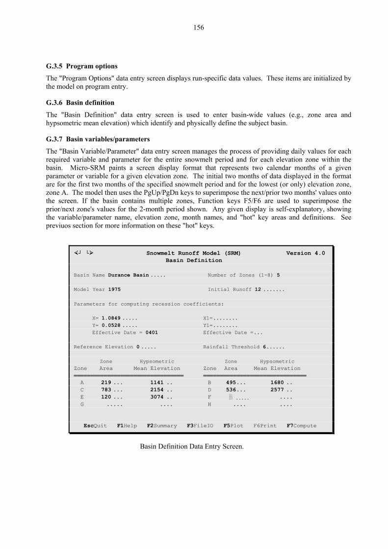
156

G.3.5 Program options

s run-sp

Th data entry screen is used to enter basin-wide values (e.g., zone area and hyp n) which identify and physica

G.3.7 Basin variables/parameters

The "Basin Variable/Parameter" data entry screen manages the process of providing daily values for each nowmel d

Micro-SRM paints a screen display format th n par . The initial two months of data displayed in the format are melt perio , zon the PgUp/PgDn keys to superimthe screen. If the basin contains multiple zones, Fun

hown. isp y is self-explanatory, showing e ation zone, month na

hese "hot" key

The "Program Options" data entry screen display ecific data values. These items are initialized by the model on program entry.

G.3.6 Basin definition

e "Basin Definition"sometric mean elevatio lly define the subject basin.

required variable and parameter for the entire s t perio and for each elevation zone within the basin. at represents two calendar months of a give

ameter or variable for a given elevation zone for the first two months of the specified snow

e sd and for the lowest (or only) elevation zone

pose the next/prior two months' values onto e A. The mod l then usection keys F5/F6 are used to superimpose the

prior/next zone's values for the 2-month period s Any given d lathe variable/p am ter name, elevar mes, and "hot" key areas and definitions. See

s. previuos section for more information on t

┘ └ Snowmelt Runoff Model (SRM) Version 4.0 Basin Definition Basin Name Durance Basin ..... Number of Zones (1-8) 5 Model Year 1975 Initial Runoff 12 ....... Parameters for computing recession coefficients: X= 1.0849 ..... X1=........ Y= ..... Y1=........ 0.0528 Effective Date = 0401 Effective Date =... Reference Elevation 0 ..... Rainfall Threshold 6...... Zone Hypsometric Zone Hypsometric Zone Area Mean Elevation Zone Area Mean Elevation ═════════════════════════════════ ═══════════════════════════════ A 219 ... 1141 .. B 495... 1680 .. C 783 ... 2154 .. D 536... 2577 .. E 120 ... 3074 .. F ░⋅ ..... .... G ..... .... H .... .... EscQuit F1Help F2Summary F3FileIO F5Plot F6Print F7Compute

Basin Definition Data Entry Screen.

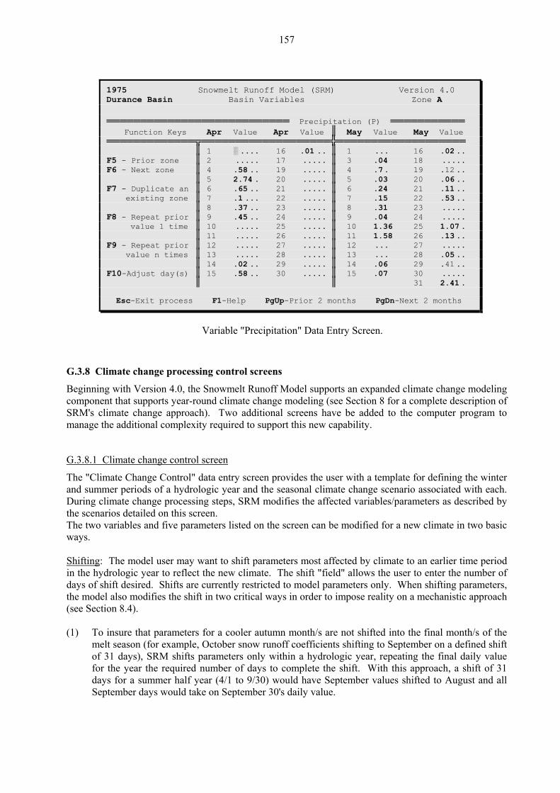
157

1975 Snowmelt Runoff Model (SRM) Version 4.0 Durance Basin Basin Variables Zone A ═══════════════════════════ Precipitation (P) ═══════════ Function Keys Apr Value Apr Value ║ May Value May Value ═════════════╦═══════════════════╬═══════════════════ ║ 1 ░ .... 16 .01 .. ║ 1 ... 16 .02 .. F5 - Prior zone ║ 2 ..... 17 ..... ║ 3 .04 18 ..... F6 - Next zone ║ 4 .58 .. 19 ..... ║ 4 .7. 19 .12 .. ║ 5 2.74 . 20 ..... ║ 5 .03 20 .06 .. F7 - Duplicate an ║ 6 .65 .. 21 ..... ║ 6 .24 21 .11 .. existing zone ║ 7 .1 ... 22 ..... ║ 7 .15 22 .53 .. ║ 8 .37 .. 23 ..... ║ 8 .31 23 ..... F8 - Repeat prior ║ 9 .45 .. 24 ..... ║ 9 .04 24 ..... value 1 time ║ 10 07 . ..... 25 ..... ║ 10 1.36 25 1. ║ 11 ..... 26 ..... ║ 11 1.58 26 .13 .. F9 - Repeat prior ║ 12 ..... 27 ..... ║ 12 ... 27 ..... value n times ║ 13 ..... 28 ..... ║ 13 ... 28 .05 .. ║ 14 .02 .. 29 ..... ║ 14 .06 29 .41 .. F10-Adjust day(s) ║ 15 .07 30 ..... .58 .. 30 ..... ║ 15 ║ 31 2.41 . ║ Esc-Exit process F1-Help PgUp-Prior 2 months PgDn-Next 2 months

Variable "Precipitation" Data Entry Screen.

G.

BecomSRma apability.

G. l screen

3.8 Climate change processing control screens

ginning with Version 4.0, the Snowmelt Runoff Model supports an expanded climate change modeling ponent that supports year-round climate change modeling (see Section 8 for a complete description of

M's climate change approach). Two additional screens have be added to the computer program to nage the additional complexity required to support this new c

3.8.1 Climate change contro

ThandDu M modifies the affected variables/parameters as described by the scenarios detailed on this screen. Thwa Sh

e "Climate Change Control" data entry screen provides the user with a template for defining the winter summer periods of a hydrologic year and the seasonal climate change scenario associated with each. ring climate change processing steps, SR

e two variables and five parameters listed on the screen can be modified for a new climate in two basic ys.

ifting: The model user may want to shift parameters most affected by climate to an earlier time period the hydrologic year to reflect the new climate. The shift "field" allows the user to enter the number of s of shift desired. Shifts are currently restricted to model parameters only. When shifting parameters, model also

in daythe modifies the shift in two critical ways in order to impose reality on a mechanistic approach (see Section 8.4).

(1)

lue.

To insure that parameters for a cooler autumn month/s are not shifted into the final month/s of the

melt season (for example, October snow runoff coefficients shifting to September on a defined shift of 31 days), SRM shifts parameters only within a hydrologic year, repeating the final daily value for the year the required number of days to complete the shift. With this approach, a shift of 31 days for a summer half year (4/1 to 9/30) would have September values shifted to August and all September days would take on September 30's daily va

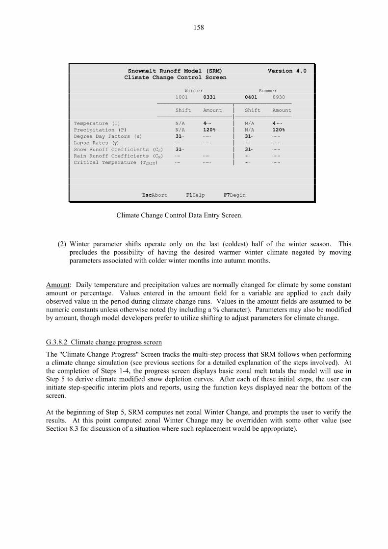
158

Snowmelt Runoff Model (SRM) Version 4.0 Climate Change Control Screen Winter Summer 1001 0331 0401 0930 ────────────────────────┬────────────────── Shift Amount │ Shift Amount ────────────────────────│────────────────── Temperature (T) N/A 4⋅⋅⋅⋅ │ N/A 4⋅⋅⋅⋅⋅ Precipitation (P) N/A 120%⋅ │ N/A 120% Degree Day Factors (a) 31⋅⋅ ⋅⋅⋅⋅⋅⋅ │ 31⋅⋅ ⋅⋅⋅⋅⋅⋅ Lapse Rates (γ) ⋅⋅⋅⋅ ⋅⋅⋅⋅⋅⋅ │ ⋅⋅⋅⋅ ⋅⋅⋅⋅⋅⋅ Snow Runoff Coefficients (CS) 31⋅⋅ │ 31⋅⋅ ⋅⋅⋅⋅⋅⋅ Rain Runoff Coefficients (CR) ⋅⋅⋅⋅ ⋅⋅⋅⋅⋅ │ ⋅⋅⋅⋅ ⋅⋅⋅⋅⋅⋅ Critical Temperature (TCRIT) ⋅⋅⋅⋅ ⋅⋅⋅⋅⋅⋅ │ ⋅⋅⋅⋅ ⋅⋅⋅⋅⋅⋅ EscAbort F1Help F7Begin

Climate Change Control Data Entry Screen.

(2) Winter parameter shifts operate only on the last (coldest) half of the winter season. This

Am

precludes the possibility of having the desired warmer winter climate negated by moving parameters associated with colder winter months into autumn months.

ount: Daily temperature and precipitation values are normally changed for climate by some constant ount or percentage. Values entered in the amount field for a variable are applied to each daily am

observed value in the period during climate change runs. Values in the amount fields are assumed to be nu eters may also be modified by adjust parameters for climate change.

G.

meric constants unless otherwise noted (by including a % character). Parammount, though model developers prefer to utilize shifting to a

3.8.2 Climate change progress screen

The "Climate Change Progress" Screen tracks the multi-step process that SRM follows when performing a ctheSteiniscr At the beginning of Step 5, SRM computes net zonal Winter Change, and prompts the user to verify the res ted zonal Winter Change may be overridden with some other value (see Section 8.3 for discussion of a situation where such replacement would be appropriate).

limate change simulation (see previous sections for a detailed explanation of the steps involved). At completion of Steps 1-4, the progress screen displays basic zonal melt totals the model will use in p 5 to derive climate modified snow depletion curves. After each of these initial steps, the user can tiate step-specific interim plots and reports, using the function keys displayed near the bottom of the een.

ults. At this point compu

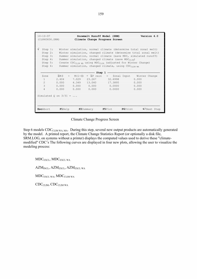
159

10-10-97 Snowmelt Runoff Model (SRM) Version 4.0 (IL840606.SRM) Climate Change Progress Screen √ Step 1: Winter simulation, normal climate (determine total zonal melt)

Step 2: Winter simulation, changed climate (determine total zonal melt) Step 3: Summer simulation, normal climate (save MDC, simulated runoff) Step 4: Summer simulation, changed climate (save MDCCLIM) Step 5: Create CDCCLIM WA using MDCCLIM (adjusted for Winter Change) Step 6: Summer simulation, changed climate, using CDCCLIM WA

────────────────────────────────── Step 1 ─────────────────────────────────

Zone ΣM⋅S + M(1-S) + ΣP_rain = Zonal Input Winter Change 1 2.404 7.029 23.267 32.6998 0.000 2 0.000 4.349 13.040 17.3895 0.000 3 0.000 0.000 0.000 0.0000 0.000 4 0.000 0.000 0.000 0.0000 0.000

Simulated Q on 3/31 = ... ───────────────────────────────────────────────────────────────────────────── EscAbort F1Help F2Summary F5Plot F6Print ┘Next Step

Climate Change Progress Screen

p 6 models CDC StebySRmomodeling process:

CLIM WA, MA. During this step, several new output products are automatically generated the model. A printed report, the Climate Change Statistics Report (or optionally a disk file, M.LOG, on systems without a printer) displays the computed values used to derive these "climate-dified" CDC’s The following curves are displayed in four new plots, allowing the user to visualize the

MDCEXCL, MDCEXCL WA

AZMINCL, AZMEXCL, AZMEXCL WA

MDCEXCL WA, MDCCLIM WA

CDCCLIM, CDCCLIM WA

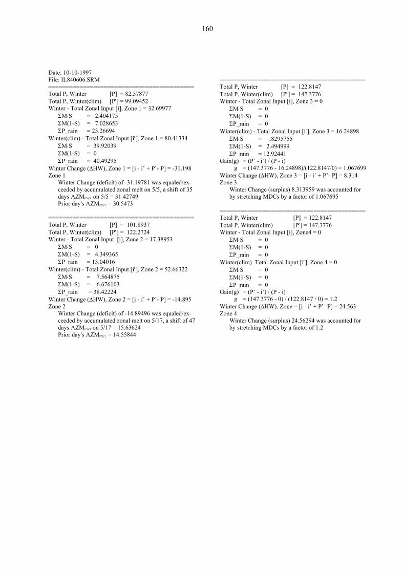
160

Date: 10-10-1997 File: IL840606.SRM ========================================== Total P, Winter [P] = 82.57877 TotWi

Wi

P_rain = 40.49295 Winter Change (Zone 1

Wicee shift of 35 days EXCL

Prio

=====Total PTotal PWinter

ΣMΣMΣP_rain = 13.04016

Winter(ΣMΣM(1-S) = 6.676103 ΣP_rain = 38.42224

Winter Change (∆HW), Zone 2 = [i - i’ + P’- P] = -14.895 Zone 2

Winter Change (deficit) of -14.89496 was equaled/ex-ceeded by accumulated zonal melt on 5/17, a shift of 47 days AZMEXCL on 5/17 = 15.63624 Prior day's AZMEXCL = 14.55844

========================================== Total P, Winter [P] = 122.8147 Total P, Winter(clim) [P′] = 147.3776

Gain(g) = (P’ - i’) / (P - i)

Winter Change (surplus) 8.313959 was accounted for by stretching MDCs by a factor of 1.067695

ΣP_rain = 0

= 0 ΣP_rain = 0

Gain(g) = (P’ - i’) / (P - i) g = (147.3776 - 0) / (122.8147 / 0) = 1.2

Winter Change (∆HW), Zone = [i - i’ + P’- P] = 24.563 Zone 4

Winter Change (surplus) 24.56294 was accounted for by stretching MDCs by a factor of 1.2

al P, Winter(clim) [P′] = 99.09452 nter - Total Zonal Input [i], Zone 1 = 32.69977 ΣM⋅S = 2.404175 ΣM(1-S) = 7.028653 ΣP_rain = 23.26694

nter(clim) - Total Zonal Input [i′], Zone 1 = 80.41334 ΣM⋅S = 39.92039

M(1-S) = 0

Winter - Total Zonal Input [i], Zone 3 = 0 ΣM⋅S = 0 ΣM(1-S) = 0 ΣP_rain = 0

Winter(clim) - Total Zonal Input [i′], Zone 3 = 16.24898 ΣM⋅S = .8295755 ΣM(1-S) = 2.494999 ΣP_rain = 12.92441 Σ

Σ∆HW), Zone 1 = [i - i’ + P’- P] = -31.198

nter Change (deficit) of -31.19781 was equaled/ex-ded by accumulated zonal melt on 5/5, a

AZM on 5/5 = 31.42749

g = (147.3776 - 16.24898)/(122.8147/0) = 1.067699 Winter Change (∆HW), Zone 3 = [i - i’ + P’- P] = 8.314 Zone 3

r day's AZMEXCL = 30.5473

===================================== , Winter [P] = 101.8937 , Winter(clim) [P′] = 122.2724 - Total Zonal Input [i], Zone 2 = 17.38953 ⋅S = 0 (1-S) = 4.349365

========================================== Total P, Winter [P] = 122.8147 Total P, Winter(clim) [P′] = 147.3776 Winter - Total Zonal Input [i], Zone4 = 0

ΣM⋅S = 0 ΣM(1-S) = 0

clim) - Total Zonal Input [i′], Zone 2 = 52.66322 ⋅S = 7.564875

Winter(clim) Total Zonal Input [i′], Zone 4 = 0 ΣM⋅S = 0 ΣM(1-S)

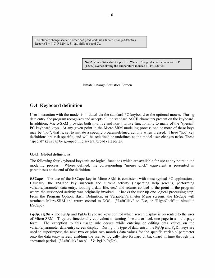
161

The climate change scenario described produced this Climate Change Statistics Report (T + 4°C, P 120 %, 31 day shift of a and CS.

Note! Zones 3-4 exhibit a positive Winter Change due to the increase in P (120%) overwhelming the temperature-induced (+ 4°C) deficit.

Climate Change Statistics Screen.

. K

Us in the standard PC keyboard or the optional mouse. During dat nt s and accepts all the standard ASCII characters present on the keyboard. In addition, Micro-SRM provides both intuitive and non-intuitive functionality to many of the "special" PC board keys. At any given point in the Micro-SRM modeling process one or more of these keys

ined activity when pressed. These "hot" key definitions are task-specific, and will be redefined or undefined as the model user changes tasks. These "special" keys c

G.4.1 Global definitions

The following four keyboard keys initiate logical functions which are available for use at any point in the

SCape - The use of the ESCape key in Micro-SRM is consistent with most typical PC applications.

activity was originally invoked. It backs the user up one logical processing step. rom the Program Option, Basin Definition, or Variable/Parameter Menu screens, the ESCape will

gUp, PgDn - The PgUp and PgDn keyboard keys control which screen display is presented to the user of ionally equivalent to turning forward or back one page in a multi-page for while entering or editing data values on the variable/param this type of data entry, the PgUp and PgDn keys are use to pecific variable/ parameter ont the ckward in time through the snowme

G 4 eyboard definition

er teraction with the model is initiated viaa e ry, the program recognize

keymay be "hot", that is, set to initiate a specific program-def

an be grouped into several broad categories.

modeling process. Where defined, the corresponding "mouse click" equivalent is presented in parentheses at the end of the definition. EBasically, the ESCape key suspends the current activity (inspecting help screens, performing variable/parameter data entry, loading a data file, etc.) and returns control to the point in the program where the suspendedFterminate Micro-SRM and return control to DOS. ("LeftClick" on Esc, or "RightClick" to simulate ESCape). P

Micro-SRM. They are functm. The exception to this usage rule occurs

eter data entry screen display. During d superimpose the next two or prior two month's data values for the so data entry screen, enabling the user to logically step forward or ba

lt period. ("LeftClick" on PgUp PgDn). ┘ └

162

Enter to terminate keyboard responses. Enter ┘ implies tha nf del, and the model should now react to that information. Mo co current input data field is complete. When pressed, the mo l dates the current field's contents for consistency, range validity, etc. (see field content validation above). Micro-SRM "remembers" each input field's most recent value, and so only initiates validation when field contents change. If the field value is unchanged or the changed value

e ext logical field on the screen display. If validation fails, an appropriate error message is displayed and

.4.2 Cursor movement keys

The keys described here are all capable of moving the screen cursor from the current data entry field to some other field in the same screen display. When that occurs, their use initiates a data validation response identical to that of the Enter ┘ key. Using these keys, the model user may move freely about the input data screen, entering new and editing existing field values. ("LeftClick" on any field to move the cursor to that field.) Movement between in ut fie rned by a forward and a backward progression eque n ( t ┘ or Tab keys) on a screen beginning at the top leftmost field, is from left to right, top to bottom. Backward progression is the reverse. Movement vertically Movement via the Enter ┘ ram y is from current day to next calendar day. Tab - The Tab key fun tions Enter ┘ {Shift}Tab - If the cursor is not on a field's first character, it shifts to the first character. If on the field's first character, the cursor moves to a prior field, as dictated by the backward progression.

ome/End - These keys move the cursor to the first/last data field, respectively, on the screen display. - Within a field value the screen cursor may be moved left or right from character to character. If

cter of the field, a "←" moves the cursor to the prior field as defined by

h the cursor advancing to

e field marked by the reverse-video cursor, and all existing characters shifted rightward. sert mode is canceled by pressing Insert again, or moving the cursor to another data field or screen.

┘ - The Enter ┘ key is used by Micro-SRMt i ormation has been provided to the most mmonly, it signals that data entry for the de optionally vali

validates successfully, the model accepts it into its internal schema and advances the screen cursor to thnthe cursor relocates to the first character of the offending field's value. When used with a menu screen display or pop-up window, the Enter ┘ key directs the model to use the menu option marked by the light bar as your choice from that menu. Enter ┘ is also used during the FileIO process to terminate a request for a filename by the model. ("LeftClick" another input field or Enter ┘).

G

p lds initiated by cursor movement key-presses is gove s nce. The forward progressio via he Enter

is generally from the current field up/down to the next closest field. key during daily variable/pa eter data entr

c exactly the same as

H↑←↓→the cursor is at the leftmost charathe screen's backward progression. If the cursor is at the rightmost character of the field value, a "→" moves the cursor to the next field in the forward progression. An "↑" or "↓" moves the cursor to the next higher/lower field relative to the current field.

G.4.3 Field editing keys

Micro-SRM uses "type-over" as its standard data entry mode. This means that any valid data character typed through the keyboard will replace that marked by the blinking cursor, witthe next character position in the field. The model supports "word-processor-like" editing via the following keys: Insert - The Insert key toggles the data entry mode to "insert", with any typed characters being inserted at he point in tht

In

163

Delete - The Delete key is logically the opposite of Insert. The character marked by the cursor is deleted, and all characters to the right of the cursor are shifted left one position. Backspace - The Backspace key deletes the character immediately to the left of the cursor, with all

is set (indicator on screen line 24 is visible), any alphabetic character ntered will appear in upper case. Press CapsLock again to turn off.

cro-SRM assumes you are entering numeric data, not ying to relocate the cursor or change the display page.

, active at that point in the program). he functions described below are Micro-SRM "primary" function key definitions. These functions are

"hot" while the "Program Options", "Basin Definition", and "Basin Variable/Parameter Menu" screens are displayed:

primary screen display (Program Option, Basin Definition, Variable/Parameter Menu, Variable/Parameter Data Entry), Micro-SRM replaces that screen display with

ally related to the user's position within the model. While help is active, the

ction is invoked by pressing/clicking function key F2 from the Program Options, riable/Parameter display screens. The Micro-SRM summary screen provides the

t) for each month in the snowmelt period are displayed for seven model parameters. Each zone in the basin is displayed

essed via the PgUp and PgDn keys. A printed version of the summary may be

figuration. ESCape - Exit function and return to point where invoke

characters at and right of the cursor shifted left one position. CapsLock - When CapsLock e NumLock - When NumLock is set (indicator is visible), characters entered through the keyboard's number pad are treated as numbers. WARNING!! If NumLock is on, the cursor movement key equivalents on the number pad are deactivated. Mitr

G.4.4 Function keys

Micro-SRM uses the microcomputer's dedicated keyboard function keys (F1-F10) to provide the user with the ability to interrupt the current model activity (typically data entry) with a single keypress/mouse click, and transfer control to a specific predefined function process. On function termination, control returns to the point of interruption. Each Micro-SRM screen display includes information on the function keys that are "hot" (i.e.T

F1-Help - The Help function is invoked by pressing/clicking function key F1 at any point in the modeling process. When help is requested from a

the Help Screen most logicuser may PgUp or PgDn to view all of Micro-SRM's available help screens. The function is terminated with an ESCape, and returns the model to the logical state existing prior to the help request. When help is requested from within another function (SUMMARY, FILEIO, PLOT, PRINT), it is presented slightly differently, through the use of a pop-up window, a transient area nondestructively superimposed over the current display image. These function pop-ups are only accessible after invoking the specific function. F2-Summary - This funBasin Definition, or Vauser with a "snapshot" of basin definition variables and zone-specific parameter values as they are currently defined. Beginning and mid-month value (day 1 and day 16 if differen

separately, and is accselected through the Print Menu (see below). The following keys are "hot" within the summary function:

F1 - Help info on this function PgUp/PgDn - - Display the next/prior zone's con

164

F3-FileIO - The File Input/Output function is invoked by pressing/clicking function key F3 from rogram Options, Basin Definition, or Variable/Parameter display screens. In response to the hot-key, a

ata from non-model sources.

Psmall "pop-up" menu is displayed. The user specifies one of four sub-options by moving the menu bar using the up arrow or down arrow, then pressing Enter ┘, pressing the desired sub-option's highlighted letter, or left-clicking on the menu selection. FileIO provides the modeler with tools to load, save and delete model data files and to import digital input d

Load - The Load option allows the user to identify and input a .SRM data file (see SAVE below) into the model. After a successful load, the model assumes a state identical to that existing when the referenced data file was created. Save - The Save option allows a user to create and name a file containing the ASCII representation of the data currently resident in the model's data structures. The file qualifier ".SRM" completes each save file's name, making it easy to recognize and manage model data. A data compression algorithm shrinks the 100K+ internal data structures into a more manageable size (a complete five zone basin

notation identical to the FORTRAN repeat count concept (IBM VS FORTRAN, 1983). might require 10K) using shorthand

Delete - This option provides the model user with the ability to delete any SRM data file (.SRM-qualified) currently residing on any of the PC's storage devices. Import - The Import option provides a method for introducing digital input data from a non-SRM source to the model. Using a simple format (press F1 for a popup describing the import format), any of the 13 model variables/ parameters detailed on the Variable/Parameter Input Data Screen may be generated externally and directly loaded into SRM. To be accessible to SRM, all import data files

st be qualified ".DAT".

panels. The upper panel displays the individual system's available devices, and lists all ctorie ames f

object using the cursor keys, then pressing Enter ┘, or by clicking on the esired object with the left-mouse-button. Alternatively, the user can press the TAB → key to switch to

board to enter the desired filename, then press Enter ┘, to select the file. ered is a valid pathname (i.e., a device {A:, B:}, directory name ending with "\",

mu

Once a FileIO option is selected, Micro-SRM displays a file selection/definition screen made up of two display subdire s and filen or the current default device/directory. The lower panel displays the current pathname (i.e., the device, directory, or filename) that will be used to attempt to fulfill the current FileIO operation. The selection screen uses two simple approaches for identifying target file names. The first approach is "point and shoot". With the upper panel "active", an object from that panel may be selected by moving he light bar to the desired t

dthe lower panel and use the keyIf the object selected/entor <Parent> the default device\ directory will be changed, and all appropriate files on the new path will be displayed. F5-Plot - The PLOT Function is invoked by pressing/clicking function key F5 from the Program Options, Basin Definition, or Variable/Parameter Menu display screens. Micro-SRM will refuse this function request and generate an appropriate error message if the PC has no graphics adapter present or a

165

simulation/forecast has not beedisplayed. The five Micro-SRM plot products available during normal processing are:

n run since last data entry. If the F5 key is "hot", the plot options menu is

Snow Depletion vs Total Snowmelt Depth

user

- Move menu bar to next/prior choice

y request a hard-copy by pressing function key F10. Press

n. Press ESCape to return to the Plot Menu. The fifth option on the menu, Build Plot File, generates an ASCII file containing all the information

bination of the Micro-SRM plot products using non-model

n key F6 from the Program Options, Basin Definition, or Variable/Parameter display screens. The print products available in Micro-SRM are:

Temperature Values

Degree Day Factors, Runoff Coefficients

Lapse Rate, Critical Temperature, Rain Contributing Area, Lag Time

Zone Degree-Days, Observed Precipitation, Snow-Covered Area (S)

Melt Depth (M ⋅ S), Melt/New Snow (M (1−S)), Contributing Rain (Cpr)

Measured vs Computed Streamflow

Snow Depletion vs Time

Accumulated Zone Melt Depth vs Time

Build External Plot File

If Micro-SRM performs a climate-change run, the state of the plot menu changes, presenting thewith the following choices:

Computed Flow Before/After Climate Change

CDC/Clim (Model Adjusted) vs Time

Build External Plot File

The following keys are "hot" while this menu is displayed:

F1 - Help for Plot Menu Up/Down Arrow Enter ┘ - Invoke selected plot option ESCape - Exit function

After a plot has been displayed, the user manter ┘ to cycle through any additional zone(s) in the basiE

necessary to recreate a user-selected comhardware/software. F6-Print - The PRINT menu is displayed by pressing/clicking functio

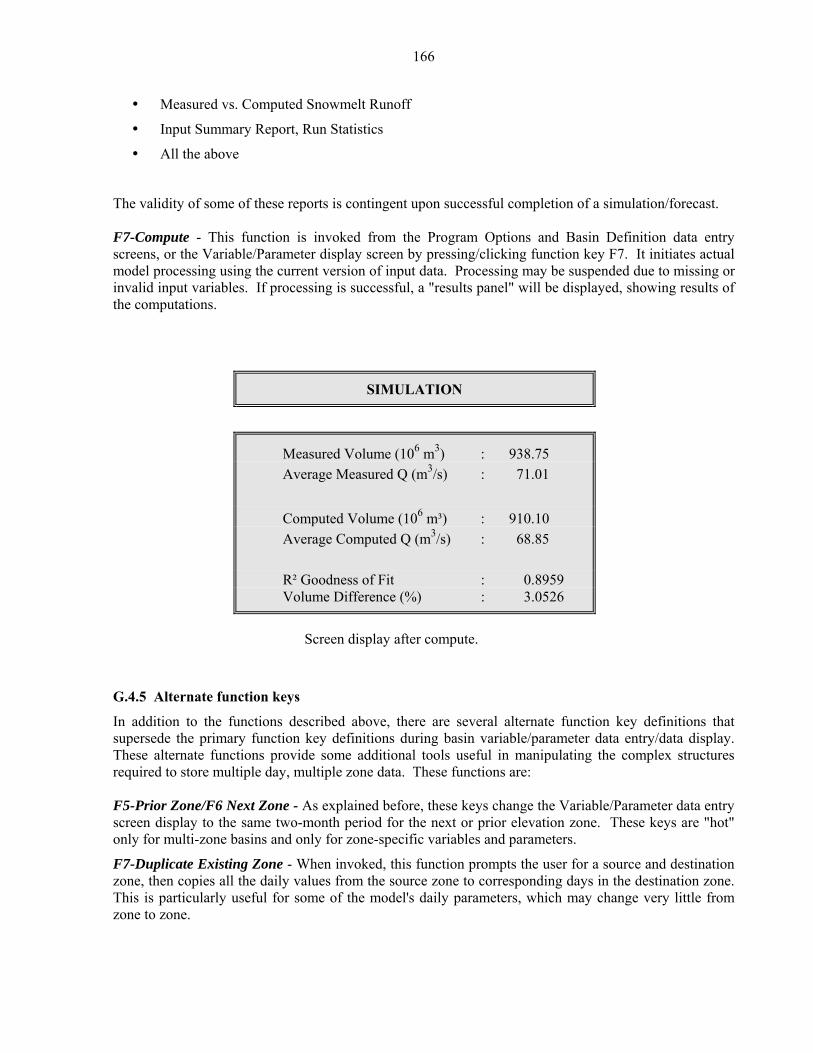
166

Measured vs. Computed Snowmelt Runoff

un Statistics

, or the Variable/Parameter display screen by pressing/clicking function key F7. It initiates actual be suspended due to missing or

layed, showing results of h

Input Summary Report, R

All the above

The validity of some of these reports is contingent upon successful completion of a simulation/forecast. F7-Compute - This function is invoked from the Program Options and Basin Definition data entry creenss

model processing using the current version of input data. Processing mayvalid input variables. If processing is successful, a "results panel" will be dispin

t e computations.

SIMULATION

Measured Volume (106 m3) : 938.75 Average Measured Q (m3/s) : 71.01

Computed Volume (106 m³) : 910.10 Average Computed Q (m3/s) : 68.85

R² Goodness of Fit : 0.8959 Volume Difference (%) : 3.0526

Screen display after compute.

are several alternate function key definitions that

corresponding days in the destination zone. This is particularly useful for some of the model's daily parameters, which may change very little from zone to zone.

G.4.5 Alternate function keys

addition to the functions described above, there Insupersede the primary function key definitions during basin variable/parameter data entry/data display. These alternate functions provide some additional tools useful in manipulating the complex structures required to store multiple day, multiple zone data. These functions are: F5-Prior Zone/F6 Next Zone - As explained before, these keys change the Variable/Parameter data entry screen display to the same two-month period for the next or prior elevation zone. These keys are "hot" only for multi-zone basins and only for zone-specific variables and parameters.

F7-Duplicate Existing Zone - When invoked, this function prompts the user for a source and destination zone, then copies all the daily values from the source zone to

167

F8-Repeat Prior Value - Pressing F8 causes the value for the day preceding that marked by the cursor to be copied into the current day position. The cursor then advances to the next day. If the cursor is on the

-sight, that is, the

ng the entire array. When invoked, the user may insert a blank day at the point marked by the cursor, shifting existing day values one day forward in time, or delete the day marked by the cursor,

antify the accuracy of the calculations. Any keypress then turns the model to its precompute state.

.5.2 Summary display

F ions for a complete description of tpconfigurations. The basin name and model run number are included, identifying the specific iterative ver ion of th

G. 3 .SRM

As escribed beforenecessary to recreate the m .

G.5.4 Plot displays

odes. Once plotted, and

M Runoff is plotted along the Y-axis (instantaneous flow), time along the X-axis. Run statistics are displayed in the upper right corner.

first day of the earlier of the two months displayed, the prior day value used is out-oflast day of month preceding the month displayed. F9-Repeat Prior Value N Times - After prompting the user for a repeat count, the model enters the value from the day preceding the cursor into the next N days, moving the cursor as it proceeds. The repeat count can vary from 1 to 365. F10-Insert/Delete Day - This function lets the user modify an existing array of daily values without reenteri

shifting existing daily values one day back in time.

G.5 Micro-SRM output products

Several different forms of output have been included in Micro-SRM, designed to support a user's specific requirements for information provided to, and generated by the model. Model output is user-selectable, and for several of the forms, interactively controlled. The available output products are described in the following paragraphs.

G.5.1 Simulation/forecast statistics

Each time an F7-Compute is successfully executed, the model suspends further processing while it displays several important statistics which qure

G

unction Key F2 invokes the model summary screen. See previous secthis function. It is designed to give the user a quick overview of the state of seven critical model arameters. Summary is useful when making iterative runs, each with slightly different parameter

s e data displayed.

5. data file

d , the FileIO menu option "Save" creates a disk file containing all the information odel run at some future time, via the "Load" function

Micro-SRM produces several different plots in one of several different screen massuming a compatible printer, a hardcopy of the plot image can be produced.

easured vs Computed Streamflow -

168

Sall specific zone, in ascending order. Press ESCape to terminate the plot. Snow Deple covered area (%) is plotted on the Y-axis, cor spondin cumulated snowmelt reduced by the effect of new snow, are plotted on the X-axis. Each zone is plotted separately. Press Enter ┘ to see the next zone, ESCape to terminate and return to the Plot Menu.

A ge) (y) is plotted against time (x). Press Enter ┘ to change zones, ESCape to terminate the plot.

e Micro-SRM's plots are saved to a user-named external disk(ette) file (.PLT-qualified). The .PLT file format is described in more detail in

G.5.4.1

now Depletion vs Time - Snow depletion curves for each zone are produced. The initial image displays the basin's snow depletion curves on a single image. Press a key to produce a separate plot of each

tion vs Total Snowmelt Depth - Daily snow re g accumulated snowmelt depth, and ac

ccumulated Zone Melt Depth vs. Time - Accumulated zone melt depth (areal covera

".PLT" Plot File - All the input and model-generated values used to creat

the sample .PLT file included on the Micro-SRM distribution diskette.

Plot displays (climate change)

ersion 4.0 and later will automatically produce several additional plot displays during climate SRM, Vchange MDCEXnew sno te conditions (the amount of melt needed to decrease the snow covered area to a certain proportion of the total). The second curve is derived from MDCEXCL by int AZMINwithoutof the iclimate. MD ct areal snow water equivalent of the initial snow cover in a cha CDC vfirst cuchange

G.5.5 Pr

Micro-SRmenu conreport setby pressibefore ESinput nor com

simulation runs.

CL vs MDCEXCL WA - The first curve depicts the snow water equivalent of the existing snow pack, w excluded, under normal clima

roducing the effect of a winter climate change upon areal snow water equivalent.

CL, AZMEXCL, AZMEXCL WA - Accumulated zonal melt curves for the melt season, with and new snow falls, and "winter-adjusted" AZM. The first two curves depict areal water equivalent nitial snow cover under normal climate conditions, the last, areal water equivalent in a changed

CEXCL WA vs MDCCLIM WA - These curves depinged climate, with and without new snow added.

s CDCCLIM WA - These curves depict snow covered area for the normal and changed climate. The rve is taken from input data provided by the user. The second curve is derived by the climate algorithms of SRM.

inted reports

M includes 7 different printed report formats, each display one or more model variable(s). The trolling selection of printed reports allows the user to select an individual report, or the entire (see previous sections for more information on the F6 print function). Printing can be canceled ng ESCape at any time during printing (if print buffering is in effect, there will be some delay Cape takes effect). Each selected report will print, even if there are no data present (i.e., neither

puted). The following reports are available:

169

TemperPrints temday in the m Options Screen .

egree-Day Factors, Runoff Coefficients aily degree-day factors (AN) and snow/rain runoff coefficients are printed for each day of the melt

period. Lapse RaParameters displayed control how discrete temperature values are applied basin-wide (lapse rate), when to p), howdis ZoA zone-temperaacross t a given day). MeIntermemelt demelted ne MeasurSimulatedVolumetr Input SuA printouprinted fo All the Above Ge ports.

G.

Version 4.0 of SRM includes one additional printed report, the Climate Change Statistics Report that pre ed to derive climate-affected snow cover.

ature Values ({form}) perature values entered by the user in the temperature form selected (max/min, mean) for each snowmelt period, as specified on the Progra

DD

te, Critical Temperature, Rainfall Contributing Area, Lag Time

treat precip as snow (critical tem to calculate the effect of precipitation (RCA), and how to tribute resulting runoff over time (lag time).

ne Degree-Days, Observed Precip, Snow-Covered Area specific report that displays DD temperature (either computed from max/min, average daily ture, or entered directly as DD's), observed precip (these values may be zone specific or apply he entire basin), and snow-covered area (% of zone covered on

lt Depth, (M ⋅ S), Melt/New Snow (M (1−S)), Precip Contributing to Runoff diate results of Micro-SRM computations. For each elevation zone, this report details daily total pth, zone contribution to runoff (M ⋅ S), and precip contributing to runoff, either as rain, or as

w-snow.

ed vs Computed Snowmelt Runoff /forecast and measured streamflow (if provided) are plotted against time. Run statistics (R², % ic Difference) are meaningful only if actual runoff values have been provided.

mmary Report, Run Statistics t of the model summary display. Bi-monthly values (1st, 16th) for 7 model parameters are r each zone in the basin. Run statistics are for the most current model run.

nerates a complete set of printed re

5.6 Printed reports (climate change)

sents the computed values us

170

storage. This hould only occur during variable/parameter data entry, where daily values may contain no more than 6

digits. The following sequence of steps describes a typical Micro-SRM session:

d changes to the program control information displayed on this screen, then presses PgDn to view the "Basin Definition" data screen.

the Basin Variable/Parameter Definition Menu.

s of the snowmelt period for the selected variable.

s PgUp or PgDn to view a different two-month slice of daily values for the same variable.

(8) The user repeats steps 5-7 for all required variables and parameters.

point during these steps the user may interrupt the data entry activity by pressing an active nction key (to request help, save data, display the data summary screen, etc.). After data entry is

plete, the simulation or forecast can be computed (press F7) and the results displayed (F5 for plots,

ply checks for the presence of a non-zero value

lues (i.e., precipitation), the model user is given the opportunity to continue the simulation or forecast, or abort processing so the "missing data" condition may be corrected.

G.6 Using Micro-SRM

Assuming the availability of the data necessary to run the model, there are only two requirements for using Micro-SRM. The target basin must contain 8 or fewer elevation zones and the physical dimensions

ay not exceed the size of the screen fields defined for their of required input data variables ms

(1) User types SRM4, then presses Enter ┘ to invoke Micro-SRM.

(2) After viewing the Introduction screen, the user presses PgDn to view the "Program Options" data screen.

(3) The user makes any require

(4) After filling the required data fields on this screen, the user begins the variable/parameter data entry process by pressing PgDn to view

(5) The user selects a variable/parameter from this menu, then presses Enter ┘ to display daily values for the first two month

(6) The user fills the daily value fields with appropriate data, then presse

(7) After data entry for the selected variable/parameter is complete, the user presses ESCape to return to the Basin Variable/Parameter Definition Menu.

t any AfucomF6 for print). Prior to each F7Compute, SRM performs a simple, "non-elegant", test to determine if all appropriate variables and parameters have been supplied by the user. For each required variable or parameter type determined by Program Option field values), SRM sim(

anywhere in the period. If any required variable or parameter fails this test, a data validation error screen is displayed that identifies the variable(s) and zone(s) that have failed the test. To view this screen, simply run Micro-SRM, enter some values on the Basin Definition Screen, and press F7Compute. Because certain model variables and parameters may legitimately contain all zero va

171

G.7 Using Micro-SRM to simulate a year-round climate change

Beginning with Version 3.11, Micro-SRM allowed a user to define a climate change scenario, a seasonal

ersion 4.0 on the effect of climate change on nowmelt ru ear (see Section 8). The original (SRM, 3.11) program′s

climate-change algorithms/processing steps have been replaced with new algorithms that model future ff. The computer program has been enhanced to manage

change, by providing a new data entry screen, the Climate hange Control Screen. This screen allows the user to easily describe climate change conditions that

al year, specifying both a winter and a summer season climate change scenario. ate change on the existing snowpack, the program can model the

and use those curves (CDCCLIM WA) during the melt

Version 4.0, a "climate-change run" is in reality five complete iteractions through the model, along

Step 1: Winter simulation, normal climate (determine total zonal melt)

• Run winter simulation with the normal climate. Compute Σwinter_zonal_meltNORMAL, where zonal melt (i) is:

M⋅S (melt from snowpack) + M⋅(1-S) (melt from newsnow) + contributing P (Cpr)

where: M = a⋅T Cpr = contributing precipitation, .i.e., that precipitation falling as rain that fell on the

snowfree area, a ripe snowpack, or a combination.)

• Determine ΣPrecipitation (P).

Step 2: Winter simulation, changed climate (determine total zonal melt) • Run winter half-year simulation with the changed climate. Compute Σwinter_zonal_meltCLIM (i’).

• Determine ΣPrecipitationCLIM (P’).

Step 3: Summer simulation, normal climate (save MDC’s, simulated runoff)

change of temperature and precipitation, and simulate its effect during the melt season. This feature was an important step in implementing the ongoing "climate-change" research that SRM model developers had conducted over the prior several years. However, we have recognized the limitation of the original climate-change algorithm, the fact that the change was isolated only on the melting season. In other words, the snowpack used during any climate change scenario was the observed real seasonal snow cover. V incorporates much of the model developers′ latest researchs noff over an entire hydrological y

snow conditions as well as climate-affected runothe steps involved in simulating climateCspan an entire hydrologic

y simulating the effect of winter climBsummer season′s climate-affected snow conditions season climate change simulation. Inwith a series of additional steps required to model climate-changed snow cover data. The program′s progress through these steps is monitored using another new screen display, the Climate Change Progress Screen. The steps defined by that screen are:

172

• Run summer simulation with the normal climate, save data needed to recreate modified depletion curves, MDCBEXCLB, accumulated zonal melt curves, AZMBEXCLB, and the simulated runoff hydrograph, QBSIM B.

MDCBEXCLB [snow depletion vs. Σ(a⋅T- newmelt)]

AZM BEXCLB [Σ((a⋅T - newmelt)⋅S) vs time]

Step 4: Summer simulation, changed climate (save MDCBCLIM B)

• Run summer simulation with the changed climate. Save Σ(a⋅T)BCLIMB, Σ(newmelt)BCLIMB.

Step 5: Derive CDCBCLIM WA Busing MDCBCLIMB (adjusted for Winter Change)

(5a) Compute ∆HBWB (Winter Change), (Σwinter_zonal_meltBNORMALB - Σwinter_zonal_meltBCLIMB, from Steps 1, 2 above).

Reduce/enhance effect of temperature-induced deficit by adding any net change to seasonal precipitation resulting from the climate change scenario. In the case of Illecillewaet, 1984, zones C and D, the scenario T + 4°C, P⋅1.2, results in a positive Winter Change ( increases in P overwhelm the winter deficit in melt). In that case, MDCBEXCLB is "stretched" rather than "cut-off", as explained in Step (5c). The Climate Change Progress Screen allows a user to over-ride a calculated zonal Winter Change value at this point in the processing sequence. See Section 8.3 for a description of when such intervention might be advisable.

(5b) For each zone, develop zonal melt curve, AZMBEXCL B(Σ(a⋅T⋅S) vs Time) for the normal climate. Find the date along AZMBEXCLB where zonal Winter Change is equaled or exceeded.

At this point, the Climate Change Statistics Report is produced. This printout (disk file if no printer is available) details the calculated values used by SRM to compute zonal Winter Change and the "cutoff" points or "gain factors" used in Step (5c) to derive MDCBEXCL WAB.

(5c) Create data for a new curve, MDCBEXCL WAB.

To understand the methodology for modeling CDCBCLIMB, it is important to understand the MDCBEXCLB curve. Each point along the curve is a daily intersection of snow water equivalent independent of melt season snowfalls (Σ (a⋅T-newmelt), and daily % snow covered area (% S), on the x-axis and y-axis respectively. The data are saved internally by SRM in ascending order, by date. SRM uses two different methodologies for creating MDCBEXCL WAB. • Methodology for winter deficits: Beginning on the date following that identified by Step (5b)

above (i.e., the "cutoff" date), all remaining daily values for MDCBEXCLB {% S and Σ (a⋅T-newmelt)} are shifted backwards in time to the beginning of the melt season. Additionally, as the curve′s x values are shifted, each daily value is reduced by a constant equal to the 1st x value following the "cutoff" date, reestablishing an x origin of 0.0. For example, if a "cutoff" date of 15 April is identified (15 days into the melt season), then all succeeding days for the data constituting the curve are shifted to the corresponding day 15 days earlier, with each daily Σ(a⋅T-newmelt) being reduced by Σ(a⋅T-newmelt)Bday 16 B.

173

• Methodology for winter surpluses (increased P overwhelms temperature increase for the zone, stretch the MDC). Compute the proportional increase in winter-ending snow water equivalent using values obtained in Steps (1-2) above:

Σ Σ

Σ Σ P - Zonal_ MeltCLIM CLIM

P- Zonal_ Melt

Multiply each x value of MDCBEXCLB by this factor to "stretch" MDCBEXCLB, creating MDCBEXCL WAB.

(5d) Derive a new curve, MDC BCLIM WAB, by adding to MDCBEXCL WAB the corresponding daily melt depths of new snow "surviving" in the warmer climate Σ(newmelt)BCLIMB from Step (4).

(5e) For each daily value, n, in MDCBEXCL WAB, find the first day on Σ(a⋅T)BCLIMB from Step (4) when the value is equaled or exceeded. Move the corresponding day’s snow cover % to day n of the CDCBCLIM WAB array. On days when multiple % S values for the same day in CDC BCLIMB result, the first (highest) value is used, the remaining values are ignored.

(5f) After all derived values have been calculated for CDCBCLIM WAB, SRM completes the new curve, CDCBCLIM WA, MAB by supplying all missing daily snow cover values using the following logic:

• Missing days that lie between two days with derived values will inherit the earlier day′s derived % S value.

• All missing days following the last derived daily value will inherit a ‘residual value’ that is determined in two different ways depending upon the difference between the last derived daily value and the corresponding value in CDC BNORMALB. The normal difference will be negative (CDCBCLIMB< CDCBNORMALB). In this situation, the residual value is set equal to the last % S value in the CDCBNORMALB. This value will typically be zero, except in cases where the zone includes a glacier or permanent snow cover. In the infrequent cases where the difference is positive (CDCBCLIMB > CDCBNORMALB) each missing daily value after the last derived day will take on the corresponding day′s % S value from CDC BNORMALB plus the difference.

(5g) Plot MDCBEXCLB, MDCBEXCL WAB.

(5h) Plot AZMBINCLB, AZMBEXCLB, AZMBEXCL WAB.

(5i) Optionally plot MDCBEXCL WAB, MDCBCLIM WAB.

(5j) Plot CDC, CDCBCLIM WAB.

(5k) Replace CDC with CDCBCLIM WA, MAB.

Step 6: Summer simulation, changed climate, using CDCBCLIM WA, MAB.

• Make one final summer "climate-change" simulation, using the existing climate-change scenario with the derived CDCBCLIM WAB curves to produce QBCLIMB.

174

After a successful climate change computation, Micro-SRM "changes state", with references to actual and simulated runoff replaced with simulated runoff before/after climate change. The "post change" data is treated as normal Micro-SRM data with the exception that it may not be used as the "base" for another climate change. If "climate-modified" data is SAVEd and reLOADed, it induces the above referenced "state change". LOADing a normal SRM file resets the model to its normal "state".

G.8 Using Micro-SRM trace file options

Several Micro-SRM command line trace options allow the advanced model user to create and use files containing the commands provided to the model via the keyboard or mouse during all or part of a program execution. This feature can prove very useful if a user is faced with the task of performing an elaborate sequence of otherwise identical processing steps on multiple years of data. By building a trace file and using a text editor to modify references to any .SRM filenames, the user insures identical processing for each year of data. In order for trace file processing to proceed in an orderly fashion, Micro-SRM makes the following assumptions when running in "trace mode":

(1) Micro-SRM processing (/TIN) begins from the same DOS path as did execution when (/TOUT) created the trace file.

(2) All pathnames and filenames referenced in a trace file exist on the PC.

During trace file creation (/TOUT={file}), each keystroke and mouse click is saved in {file}. Trace file creation can be terminated at any point in the model session by pressing ALT_@. When the model runs under control of a trace file (/TIN={file}), the program reads and processes one command from the trace file every ½ second unless the /TDELAY option is included to specify the time increment. This control sequence will continue until one of the following three trace ending events occurs: End of Program - the trace file includes the keystrokes necessary to end execution of Micro-SRM. End of Trace File - When the last command is removed from the trace file, a message is displayed and program control is returned to the keyboard and mouse. Trace Suspended - the user may suspend trace file processing by pressing Esc. After suspension, the user may optionally continue trace file processing, with the same or a modified trace delay, or terminate trace file processing at the suspension point, with control returning to the keyboard and mouse.

175

G.9 Micro-SRM availability

The Hydrology Laboratory supports and distributes the Snowmelt Runoff Model free of charge to any interested party. The program and related files are available via the Internet by accessing the SRM home page at HTUhttp://www.ars.usda.gov/Services/docs.htm?docid=8872UTH. This site also includes an electronic version of the SRM User’s Manual. A distribution diskette, available on either 5¼" or 3½" media, containing the executable code, supporting files, and example data files can be provided upon request.. To obtain the latest version of Micro-SRM, contact: USDA-ARS, Hydrology and Remote Sensing Laboratory Bldg. 007, Room 104, BARC-W 10300 Baltimore Avenue Beltsville, MD 20705-2350 USA (301) 504-7490

or via electronic mail to: [email protected] [email protected]

Micro-SRM has been distributed to several hundred individuals and institutions worldwide since 1985. We appreciate the feedback we receive from users of Micro-SRM, both positive and negative, and view it as a valuable resource in the process of debugging and improving the software.

New Mexico State University is an equal opportunity/affirmative action employer and educator. NMSU and the U.S. Department of Agriculture cooperating.

j. martinec, a. rango, r. roberts snowmelt runoff...

Documents