effects of frozen soil on snowmelt runoff and soil water ...effects of frozen soil on snowmelt...

Effects of Frozen Soil on Snowmelt Runoff and Soil Water Storage at aContinental Scale

GUO-YUE NIU AND ZONG-LIANG YANG

Department of Geological Sciences, Jackson School of Geosciences, The University of Texas at Austin, Austin, Texas

(Manuscript received 20 September 2005, in final form 14 January 2006)

ABSTRACT

The presence of ice in soil dramatically alters soil hydrologic and thermal properties. Despite thisimportant role, many recent studies show that explicitly including the hydrologic effects of soil ice in landsurface models degrades the simulation of runoff in cold regions. This paper addresses this dilemma byemploying the Community Land Model version 2.0 (CLM2.0) developed at the National Center for At-mospheric Research (NCAR) and a simple TOPMODEL-based runoff scheme (SIMTOP). CLM2.0/SIMTOP explicitly computes soil ice content and its modifications to soil hydrologic and thermal properties.However, the frozen soil scheme has a tendency to produce a completely frozen soil (100% ice content)whenever the soil temperature is below 0°C. The frozen ground prevents infiltration of snowmelt or rainfall,thereby resulting in earlier- and higher-than-observed springtime runoff. This paper presents modificationsto the above-mentioned frozen soil scheme that produce more accurate magnitude and seasonality of runoffand soil water storage. These modifications include 1) allowing liquid water to coexist with ice in the soilover a wide range of temperatures below 0°C by using the freezing-point depression equation, 2) computingthe vertical water fluxes by introducing the concept of a fractional permeable area, which partitions themodel grid into an impermeable part (no vertical water flow) and a permeable part, and 3) using the totalsoil moisture (liquid water and ice) to calculate the soil matric potential and hydraulic conductivity. Theperformance of CLM2.0/SIMTOP with these changes has been tested using observed data in cold-regionriver basins of various spatial scales. Compared to the CLM2.0/SIMTOP frozen soil scheme, the modifiedscheme produces monthly runoff that compares more favorably with that estimated by the University ofNew Hampshire–Global Runoff Data Center and a terrestrial water storage change that is in closer agree-ment with that measured by the Gravity Recovery and Climate Experiment (GRACE) satellites.

1. Introduction

Frozen soil occupies 55%–60% of the land surface ofthe Northern Hemisphere in winter (Zhang et al. 1999).It has tremendous impacts on ecosystem diversity andproductivity. Seasonal freezing and thawing of soil canaffect the decomposition of organic substances and themigratory patterns and physiology of biota living in thesoil. Greenhouse gases released from the land surfacecan be dramatically increased after the spring thaw.Frozen soil also plays an important role in the climatesystem by altering soil thermal and hydrological prop-erties. Freezing of soil water delays the winter coolingof the land surface, and thawing of the frozen soil de-

lays the summer warming of the land surface (Poutou etal. 2004). Frozen soil also affects the snowmelt runoffand soil hydrology by reducing the soil permeability.Runoff from the Arctic river systems is about 50% ofthe net flux of freshwater to the Arctic Ocean (Barryand Serreze 2000). This is a large percentage whencompared to the freshwater inputs to the tropicaloceans, where freshwater input is dominated by pre-cipitation. Runoff affects ocean salinity and sea ice con-ditions (McDonald et al. 1999; Peterson et al. 2002).The degree of surface freshening can affect the globalthermohaline circulation (Aagaard and Carmack 1989;Broecker 1997). A realistic representation of the ther-mal and hydraulic properties of frozen soil will benefitglobal and regional climate studies.

Land surface models (LSMs) for use in climate stud-ies showed much larger scatter in simulating runoff andsoil moisture in spring than in other seasons at Valdai,Russia, due to the uncertainties in representing the ef-

Corresponding author address: Dr. Guo-Yue Niu, Departmentof Geological Sciences, The University of Texas at Austin, Austin,TX 78712.E-mail: [email protected]

OCTOBER 2006 N I U A N D Y A N G 937

© 2006 American Meteorological Society

JHM538

fects of frozen soil on infiltration and runoff generation(Luo et al. 2003). Even when given the same volume ofsnowmelt water as input, different LSMs produced to-tally different runoff in terms of timing and magnitude.Earlier LSMs that did not explicitly solve soil ice con-tent parameterized the hydraulic conductivity as a stepfunction of soil temperature and switched off infiltra-tion for subfreezing temperatures (Xue et al. 1991;Yang and Dickinson 1996). This treatment failed toproduce the spring peaks of soil moisture due to theunderestimated infiltration of snowmelt water (Robocket al. 1995; Xue et al. 1996). Xue et al. (1996) improvedtheir LSM’s ability to simulate the spring peaks of soilmoisture by gradually decreasing the hydraulic conduc-tivity at a rate of 10% per degree for subfreezing tem-peratures following SiB2 (Sellers et al. 1996). Pitman etal. (1999) implemented an explicit representation of thehydrological and thermal effects of soil ice in their LSMbut found that the representation degraded runoffsimulation in a large-scale river basin. They suggestedLSMs should not include the effects of soil ice on runoffuntil more observations at various scales are available.

Field studies in the literature also revealed conflict-ing results about the effects of frozen soil on infiltrationand runoff generation. The field studies in local-scaleopen areas showed that the soil infiltration capacity isnormally reduced by the presence of ice, which maygenerate considerable surface runoff and decrease theunderlying groundwater recharge (Dunne and Black1971; Kane and Stein 1983; Bengtsson et al. 1992; Sta-dler et al. 1996). However, Russian laboratory and fieldstudies in 1960s and 1970s showed that there are weakor no clear effects of frozen soil on infiltration andrunoff generation especially in forested areas. Koren(1980) used these results to formulate the frozenground component of a rainfall–runoff model. Morerecent field studies in forested areas supported the Rus-sian studies (Shanley and Chalmers 1999; Nyberg et al.2001; Lindstrom et al. 2002; Bayard et al. 2005). Shan-ley and Chalmers (1999) showed that the effects of fro-zen soil on runoff are scale dependent. There was nosignificant correlation between seasonal runoff ratiosand ground frost depth for the 15 yr of record from theSleepers River watershed, United States, with an areaof 111 km2, while the increased runoff due to frozenground was observed occasionally in its 0.59-km2 agri-cultural subcatchment. Lindstrom et al. (2002) also con-cluded that there were no clear effects of frozen soil onthe timing and magnitude of runoff from an analysis of16-yr data in a 0.5-km2 watershed in northern Sweden.Researchers (Stadler et al. 1997; Stähli et al. 1999; Ny-berg et al. 2001) have demonstrated that soil structure,air-filled porosity, ice content, and the number of freez-

ing and thawing cycles are the governing factors affect-ing the infiltration capacity of frozen soil. Even at verylocal scales, recent laboratory and field studies usingdye tracer techniques (Flury et al. 1994; Stadler et al.2000; Stähli et al. 2004) revealed that water can infil-trate into deeper soil through preferential pathwayswhere air-filled macropores exist at the time of freez-ing.

One-dimensional numerical models using the fullycoupled heat and mass balance equations (Flerchingerand Saxton 1989; Zhao and Gray 1997; Cox et al. 1999;Koren et al. 1999; Stähli et al. 2001; Cherkauer andLettenmaier 2003; Hansson et al. 2004) showed a vari-ety of ways to parameterize the hydraulic properties offrozen soil. Most of these models introduced the con-cept of supercooled soil water, which is the liquid waterthat coexists with ice over a wide range of temperaturesbelow 0°C, by applying the freezing-point depressionequation. Some of the models (Flerchinger and Saxton1989; Cox et al. 1999; Hansson et al. 2004) assume thatthe freezing–thawing process is similar to the drying–wetting process with regard to the dependence of thesoil matric potential on the liquid water content. Thisassumption leads to a very low infiltration rate or evenupward water movements resulting in ice heave in sur-face layers (Hansson et al. 2004). Spaans and Baker(1996) demonstrated the validity of this assumption.But it may be only applicable to very local scale, fine-textured soil. However, other modelers (Zhao andGray 1997; Koren et al. 1999; Stähli et al. 2001;Cherkauer and Lettenmaier 2003) proposed quite dif-ferent schemes to compute hydraulic properties as ameans to produce greater infiltration rates. Stähli et al.(2001) proposed two separate domains for the waterinfiltration into frozen soil: the low-flow domain wherewater flows through the liquid water film absorbed bythe soil particles and the high-flow domain where waterflows through the air-filled macropores. Koren et al.(1999) assumed that frozen soil is permeable due to soilstructural aggregates, cracks, dead root passages, andworm holes, and used the total water content (frozenand unfrozen) in the Clapp–Hornberger relationshipsin a land model for use in a weather prediction model.Cherkauer and Lettenmaier (2003) assumed that sur-face water tends to find areas of higher infiltration ca-pacity as it flows across a frozen surface. They split theirmodel domain into 10 bins, each having different icecontent that they derived from the observed spatial dis-tribution of soil temperature, to increase the infiltrationrate in a macroscale hydrologic model. This treatmentperforms fairly well in large-scale cold-region rivers (Suet al. 2005).

The National Center for Atmospheric Research

938 J O U R N A L O F H Y D R O M E T E O R O L O G Y VOLUME 7

(NCAR) Community Land Model (CLM) (Oleson etal. 2004) introduced a frozen soil scheme in which thefreezing–thawing processes are analogous to those insnow (appendix A). The ice fraction of a soil layer be-comes 100% when the heat content is sufficient tofreeze all the liquid water. In addition, the hydraulicconductivity for frozen soil is parameterized as a func-tion of the liquid water using the Clapp–Hornbergerrelationships (Clapp and Hornberger 1978). Whenthere is no liquid water, the soil permeability becomesso low that most of the snowmelt water flows laterallyas surface runoff, resulting in a much earlier and higher-peaked spring runoff than that estimated by the Uni-versity of New Hampshire–Global Runoff Data Center(UNH-GRDC). In this study, we modified the frozensoil scheme by introducing the surpercooled soil waterand a fractional permeable area, which is parameter-ized as an exponential function of the ice content toincrease infiltration rate.

2. Model description

In this study, we use a modified version of CLM2.0,in which a simple TOPMODEL-based runoff scheme(SIMTOP; appendix B) (Niu et al. 2005) was imple-mented into the standard CLM2.0 (Bonan et al. 2002).CLM2.0 computes soil temperature and soil water in 10soil layers to a depth of 3.43 m. The thermal and hy-draulic properties of frozen soil of the standardCLM2.0 are described in detail in appendix A. Here wedescribe the modifications to the CLM2.0 frozen soilscheme.

a. Implementation of the supercooled soil water

When soil water freezes, the water closest to soil par-ticles remains in liquid form due to the absorptive andcapillary forces exerted by soil particles. This super-cooled soil water at subfreezing temperatures is equiva-lent to a depression of the freezing point. We show inthe followings how a freezing-point depression equa-tion is derived and how this equation relates to that inKoren et al. (1999).

When ice is present, soil water potential remains inequilibrium with the vapor pressure over pure ice. Whenneglecting the soil water osmotic potential, the soil wa-ter matric potential �(T)(mm) for each soil layer is

��T� �103Lf �T � Tfrz�

gT, �1�

where T and Tfrz are soil temperature and freezingpoint (K), respectively (Fuchs et al. 1978); Lf is thelatent heat of fusion (J kg�1); and g is the gravitational

acceleration (m s�2). Spaans and Baker (1996) demon-strated that freezing–thawing processes are similar todrying–wetting processes with regard to the depen-dence of the soil matric potential on liquid water con-tent. The soil matric potential as a function of liquidwater content, �(�liq), is

��liq� � �sat��liq

�sat��b

, �2�

where �sat and �liq are porosity and the partial volumeof liquid water, �sat (mm) is the saturated soil matricpotential depending on the soil texture, and b is theClapp–Hornberger parameter. By equating �(T) in Eq.(1) to �(�liq) in Eq. (2), we derive the expression for thefreezing-point depression equation:

�liq,max � �sat�103Lf �T � Tfrz�

gT�sat��1�b

, �3�

where �liq,max is the maximum liquid water when thesoil temperature is below the freezing point. Severalresearchers (Flerchinger and Saxton 1989; Zhao andGray 1997; Cox et al. 1999; Cherkauer and Lettenmier2003) have used this equation in the studies of waterflow in frozen soil. The above equation defines the up-per limit of the liquid water content for subfreezingtemperatures. Additional water may be ice dependingon the available energy. Thus, the liquid water contentfor the next time step (N � 1) follows:

�liqN�1 � min��liq,max, �N�, �4�

where �N is the total volumetric soil moisture at timestep N, including liquid water content and ice content.In the new formulation for frozen soil, Eq. (A10) inCLM2.0 for ice content (�ice) is then modified as

�ice

N � 1 � min��N � �liqN�1, �ice

N � Rfm�t�. �5�

Koren et al. (1999) proposed an alternative method forrepresenting the maximum supercooled soil water byiteratively solving the following equation, a variant ofthe freezing-point depression equation:

�1 � 8�ice�2�sat��liq,max

�sat��b

�103Lf �T � Tfrz�

gT, �6�

where the (1 � 8�ice)2 term accounts for the increasedinterface between soil particles and liquid water due tothe increase of ice crystals.

Figure 1a shows that there is a considerable amountof liquid water (0.1 m3 m�3 or more) when the soiltemperature is well below 0°C for various clay percent-ages. When the soil is assumed at saturation, hence�ice � �sat � �liq,max, Eq. (6) produces about 0.06 m3 m�3

more liquid water than does Eq. (3). The parameters b,


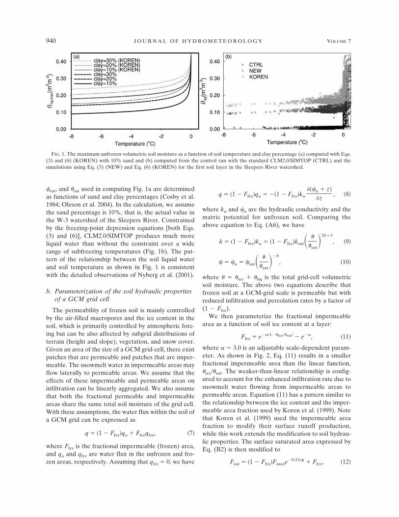
�sat, and �sat used in computing Fig. 1a are determinedas functions of sand and clay percentages (Cosby et al.1984; Oleson et al. 2004). In the calculation, we assumethe sand percentage is 10%, that is, the actual value inthe W-3 watershed of the Sleepers River. Constrainedby the freezing-point depression equations [both Eqs.(3) and (6)], CLM2.0/SIMTOP produces much moreliquid water than without the constraint over a widerange of subfreezing temperatures (Fig. 1b). The pat-tern of the relationship between the soil liquid waterand soil temperature as shown in Fig. 1 is consistentwith the detailed observations of Nyberg et al. (2001).

b. Parameterization of the soil hydraulic propertiesof a GCM grid cell

The permeability of frozen soil is mainly controlledby the air-filled macropores and the ice content in thesoil, which is primarily controlled by atmospheric forc-ing but can be also affected by subgrid distributions ofterrain (height and slope), vegetation, and snow cover.Given an area of the size of a GCM grid-cell, there existpatches that are permeable and patches that are imper-meable. The snowmelt water in impermeable areas mayflow laterally to permeable areas. We assume that theeffects of these impermeable and permeable areas oninfiltration can be linearly aggregated. We also assumethat both the fractional permeable and impermeableareas share the same total soil moisture of the grid cell.With these assumptions, the water flux within the soil ofa GCM grid can be expressed as

q � �1 � Ffrz�qu � Ffrzqfrz, �7�

where Ffrz is the fractional impermeable (frozen) area,and qu and qfrz are water flux in the unfrozen and fro-zen areas, respectively. Assuming that qfrz � 0, we have

q � �1 � Ffrz�qu � ��1 � Ffrz�ku

��u � z�

�z, �8�

where ku and �u are the hydraulic conductivity and thematric potential for unfrozen soil. Comparing theabove equation to Eq. (A6), we have

k � �1 � Ffrz�ku � �1 � Ffrz�ksat� �

�sat�2b�3

, �9�

� � �u � �sat� �

�sat��b

, �10�

where � � �ice � �liq is the total grid-cell volumetricsoil moisture. The above two equations describe thatfrozen soil at a GCM-grid scale is permeable but withreduced infiltration and percolation rates by a factor of(1 � Ffrz).

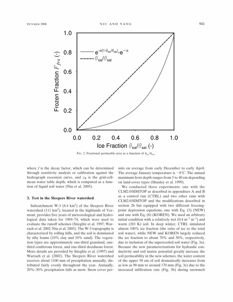
We then parameterize the fractional impermeablearea as a function of soil ice content at a layer:

Ffrz � e��1��ice��sat� � e��, �11�

where � � 3.0 is an adjustable scale-dependent param-eter. As shown in Fig. 2, Eq. (11) results in a smallerfractional impermeable area than the linear function,�ice/�sat. The weaker-than-linear relationship is config-ured to account for the enhanced infiltration rate due tosnowmelt water flowing from impermeable areas topermeable areas. Equation (11) has a pattern similar tothe relationship between the ice content and the imper-meable area fraction used by Koren et al. (1999). Notethat Koren et al. (1999) used the impermeable areafraction to modify their surface runoff production,while this work extends the modification to soil hydrau-lic properties. The surface saturated area expressed byEq. (B2) is then modified to

Fsat � �1 � Ffrz�Fmaxe�0.5fz� � Ffrz, �12�

FIG. 1. The maximum unfrozen volumetric soil moisture as a function of soil temperature and clay percentage (a) computed with Eqs.(3) and (6) (KOREN) with 10% sand and (b) computed from the control run with the standard CLM2.0/SIMTOP (CTRL) and thesimulations using Eq. (3) (NEW) and Eq. (6) (KOREN) for the first soil layer in the Sleepers River watershed.


where f is the decay factor, which can be determinedthrough sensitivity analysis or calibration against thehydrograph recession curve, and z� is the grid-cell-mean water table depth, which is computed as a func-tion of liquid soil water (Niu et al. 2005).

3. Test in the Sleepers River watershed

Subcatchment W-3 (8.4 km2) of the Sleepers Riverwatershed (111 km2), located in the highlands of Ver-mont, provides five years of meteorological and hydro-logical data taken for 1969–74, which were used toevaluate the runoff schemes (Stieglitz et al. 1997; War-rach et al. 2002; Niu et al. 2005). The W-3 topography ischaracterized by rolling hills, and the soil is dominatedby silty loams (10% clay and 10% sand). The vegeta-tion types are approximately one-third grassland, one-third coniferous forest, and one-third deciduous forest.More details are provided by Stieglitz et al. (1997) andWarrach et al. (2002). The Sleepers River watershedreceives about 1100 mm of precipitation annually, dis-tributed fairly evenly throughout the year. Annually,20%–30% precipitation falls as snow. Snow cover per-

sists on average from early December to early April.The average January temperature is �8°C. The annualmaximum frost depth ranges from 5 to 40 cm dependingon land-cover types (Shanley et al. 1999).

We conducted three experiments: one with theCLM2.0/SIMTOP as described in appendixes A and Bas a control run (CTRL) and two other runs withCLM2.0/SIMTOP and the modifications described insection 2b but equipped with two different freezing-point depression equations, one with Eq. (3) (NEW)and one with Eq. (6) (KOREN). We used an arbitraryinitial condition with a relatively wet (0.4 m–3 m–3) andwarm (283 K) soil. In deep winter, CTRL simulatedalmost 100% ice fraction (the ratio of ice to the totalsoil water), while NEW and KOREN largely reducedthe ice fraction to about 70% and 50%, respectively,due to inclusion of the supercooled soil water (Fig. 3a).Because the new parameterizations for hydraulic con-ductivity and soil matric potential greatly increase thesoil permeability in the new schemes, the water contentof the upper 50 cm of soil dramatically increases fromas low as 90 mm to around 170 mm (Fig. 3c) due to theincreased infiltration rate (Fig. 3b) during snowmelt

FIG. 2. Fractional permeable area as a function of �ice/�sat.


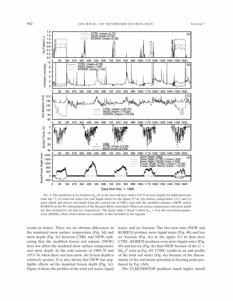
events in winter. There are no obvious differences inthe simulated snow surface temperature (Fig. 3d) andsnow depth (Fig. 3e) between CTRL and NEW, indi-cating that the modified frozen soil scheme (NEW)does not affect the modeled snow surface temperatureand snow depth. In the cold seasons of 1969–70 and1973–74, when there was less snow, the frozen depth isrelatively greater. It is also shown that NEW has neg-ligible effects on the modeled frozen depth (Fig. 3e).Figure 4 shows the profiles of the total soil water, liquid

water, and ice fraction. The two new runs (NEW andKOREN) produce more liquid water (Fig. 4b) and lessice fraction (Fig. 4c) in the upper 0.5 m than doesCTRL. KOREN produces even more liquid water (Fig.4b) and less ice (Fig. 4c) than NEW because of the (1 �8�ice)2 term in Eq. (6). CTRL results in an odd profileof the total soil water (Fig. 4a) because of the discon-tinuity of the soil matric potential at freezing point pro-duced by Eq. (A8).

The CLM2/SIMTOP produces much higher runoff

FIG. 3. The modeled (a) ice fraction (�ice/�) of the first soil layer with a 0.0175-m layer depth, (b) infiltration rate(mm day–1), (c) total soil water (ice and liquid water) in the upper 0.5 m, (d) surface temperature (°C), and (e)snow depth and frozen soil depth from the control run (CTRL) and with the modified schemes (NEW and/orKOREN) in the W3 subcatchment of the Sleepers River watershed. Observed surface temperature and snow depthare also included in (d) and (e), respectively. The mean value (“mean”) when �ice 0 or the root-mean-square-error (RMSE) when observations are available is also included in the legends.


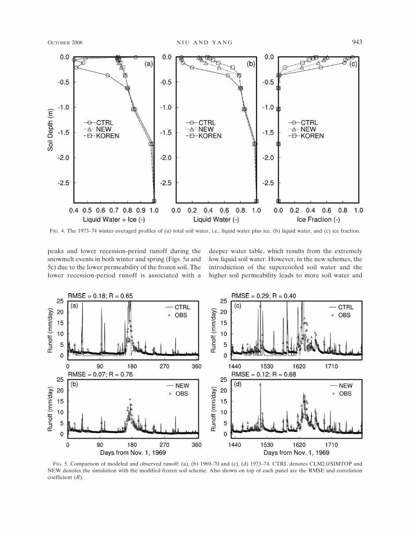
peaks and lower recession-period runoff during thesnowmelt events in both winter and spring (Figs. 5a and5c) due to the lower permeability of the frozen soil. Thelower recession-period runoff is associated with a

deeper water table, which results from the extremelylow liquid soil water. However, in the new schemes, theintroduction of the supercooled soil water and thehigher soil permeability leads to more soil water and

FIG. 5. Comparison of modeled and observed runoff: (a), (b) 1969–70 and (c), (d) 1973–74. CTRL denotes CLM2.0/SIMTOP andNEW denotes the simulation with the modified frozen soil scheme. Also shown on top of each panel are the RMSE and correlationcoefficient (R).

FIG. 4. The 1973–74 winter-averaged profiles of (a) total soil water, i.e., liquid water plus ice, (b) liquid water, and (c) ice fraction.


thus a shallower water table, which in turn producesmore subsurface runoff in the recession period (Figs. 5band 5d).

Given the fact that CLM2.0/SIMTOP with Eq. (6)produces more liquid water than does CLM2.0/SIMTOP with Eq. (3), one wonders whether the newparameterizations of the soil hydraulic properties as de-scribed in section 2b could be dropped in the KORENrun. Additional experiments show that the CLM2.0/SIMTOP equipped with Eq. (6) only still produceslower-than-observed runoff in recession period.

Because NEW and KOREN produce similar simula-tions of the total soil water storage and runoff, we willjust use the NEW scheme in the global tests.

4. Test in the six largest river basins in coldregions

To drive the model at a global scale, we used the Glob-al Land Data Assimilation System (GLDAS) 1° 1°3-hourly, near-surface meteorological data for the years2002–04 (Rodell et al. 2004a). These forcing data areobservation-derived fields including precipitation, airtemperature, air pressure, specific humidity, shortwaveand longwave radiation, and wind speed. The reason wechose the GLDAS forcing data is that they cover thesame period during which the terrestrial water storagechange measured by the Gravity Recovery and ClimateExperiment (GRACE) satellites is available. The veg-etation and soil parameters at 1° 1° were interpolatedfrom the higher-resolution raw data of CLM2.0, whichwere also used in the studies of Bonan et al. (2002) andNiu et al. (2005). The model-simulated 3-yr-averagedrunoff and snow depth were validated against themonthly UNH-GRDC runoff climatology and the U.S.Air Force Environmental Technical Applications Cen-ter (USAF-ETAC) snow depth climatology, respec-tively. The UNH-GRDC monthly composite runoffdataset combined observed river discharge with outputfrom a water balance model that was driven by ob-served meteorological data. This dataset preserves theaccuracy of the observed discharge measurements andmaintains the spatial and temporal distribution of simu-lated runoff, thereby providing the “best estimate” ofterrestrial runoff over large domains (Fekete et al.2000). The monthly USAF-ETAC global snow depthclimatology (Foster and Davy 1988) was compiled fromground-referenced measurements of snow depth. Thesix largest river basins in cold regions, that is, the Lena,Yenisei, Mackenzie, Ob, Churchill–Nelson, and AmurRiver basins, selected in this study are mostly in Russiaand North America, where Foster and Davy (1988)rated the snow depth data as having high confidencelevels.

To reduce the uncertainties induced by the initialconditions of the soil moisture and temperature, wefirst ran the model for three years from 2002 to 2004and saved the model prognostic variables including soilmoisture and temperature at the end of the model run.We used the saved model prognostic variables as theinitial conditions for another 3-yr run from 2002 to2004.

We conducted two experiments: one with CLM2.0/SIMTOP (CTRL) and one with CLM2.0/SIMTOPequipped with the modifications to the hydraulic prop-erties described in section 2b and the freezing-pointdepression Eq. (3) (NEW). In both the experiments,the runoff decay factor f � 4.0 m�1. The 3-yr averagedrunoff simulated from the NEW experiment greatly im-proves over that from CLM2.0/SIMTOP for all the sixriver basins (Fig. 6). CTRL consistently produced ear-lier and higher peaks in spring (March, April, and May)and less runoff in summer than the UNH-GRDC runoffclimatology. This is mainly because the low soil perme-ability induced by the excessive surface soil ice contentenhances surface runoff in spring. However, the snowdepth simulated by CTRL is very similar to the USAF-ETAC snow depth climatology except for YeniseiRiver and Ob River basins, where snowmelt occurseven later than observations (Fig. 6). This excludes thepossibility that the higher and earlier peaks of the simu-lated runoff result from earlier snowmelt. The modifiedscheme (NEW) largely improves the runoff simulationboth in magnitude and seasonality (Fig. 6). However,these modifications to the frozen soil scheme do notaffect the simulation of snow depth (Fig. 7).

As mentioned before, the UNH-GRDC runoffdataset is a composite product of runoff simulated by awater balance model constrained by those disaggre-gated from the observed river discharges includingR-ArcticNet (see http://www.r-arcticnet.sr.unh.edu/v3.0/main.html). Although a no-time-delay assumptionis applied when the gauge-observed discharge is distrib-uted uniformly over a catchment, the resulting runofffields over a large river basin may approximate the realrunoff when there are adequate gauges within the largeriver basin. This may explain why UNH-GRDC runoffoccurs earlier than the R-ArcticNet river dischargeswith greater values in spring (especially in May) con-sistently in Lena, Yenisei, Mackenzie, and Ob Rivers(Fig. 6). The cold-season (December–March) runoffsimulated by the modified scheme (NEW) is abouttwice as large as the GRDC runoff, but it is still lessthan the estimates derived from the R-ArcticNet riverdischarges most obviously in Yenisei, Mackenzie, andOb Rivers. Ye et al. (2003) and Yang et al. (2004) pro-vided an explanation that the higher winter R-ArcticNet


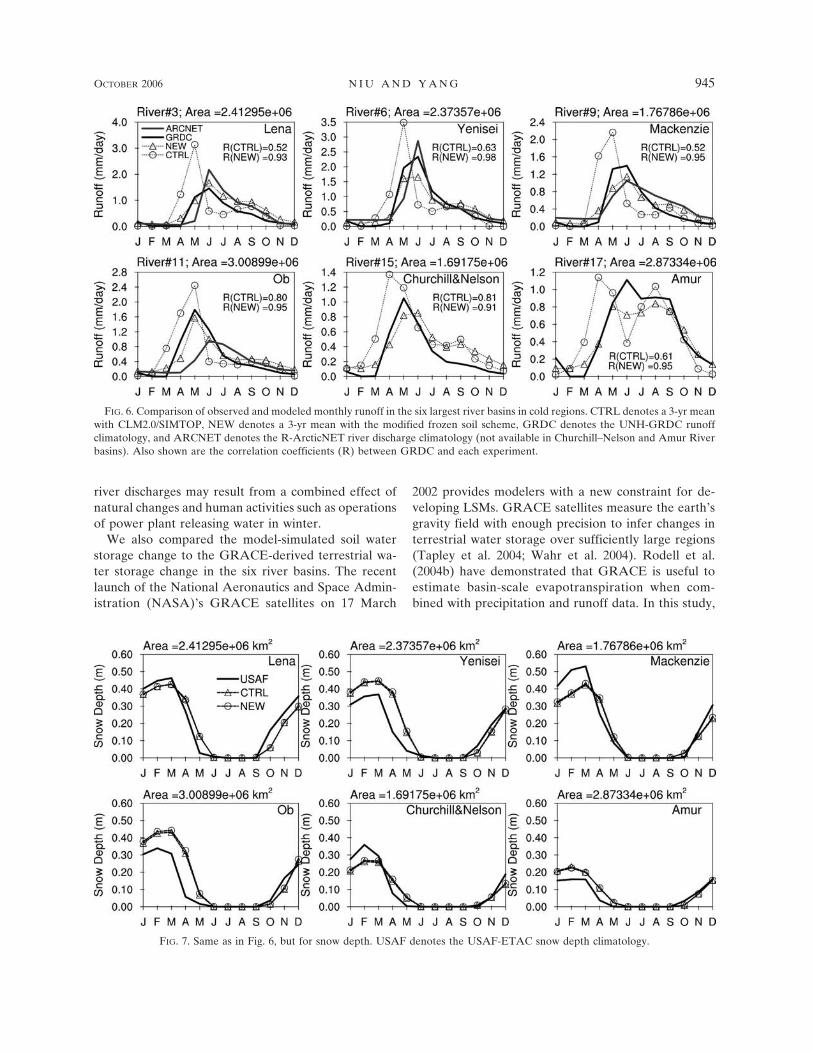
river discharges may result from a combined effect ofnatural changes and human activities such as operationsof power plant releasing water in winter.

We also compared the model-simulated soil waterstorage change to the GRACE-derived terrestrial wa-ter storage change in the six river basins. The recentlaunch of the National Aeronautics and Space Admin-istration (NASA)’s GRACE satellites on 17 March

2002 provides modelers with a new constraint for de-veloping LSMs. GRACE satellites measure the earth’sgravity field with enough precision to infer changes interrestrial water storage over sufficiently large regions(Tapley et al. 2004; Wahr et al. 2004). Rodell et al.(2004b) have demonstrated that GRACE is useful toestimate basin-scale evapotranspiration when com-bined with precipitation and runoff data. In this study,

FIG. 7. Same as in Fig. 6, but for snow depth. USAF denotes the USAF-ETAC snow depth climatology.

FIG. 6. Comparison of observed and modeled monthly runoff in the six largest river basins in cold regions. CTRL denotes a 3-yr meanwith CLM2.0/SIMTOP, NEW denotes a 3-yr mean with the modified frozen soil scheme, GRDC denotes the UNH-GRDC runoffclimatology, and ARCNET denotes the R-ArcticNET river discharge climatology (not available in Churchill–Nelson and Amur Riverbasins). Also shown are the correlation coefficients (R) between GRDC and each experiment.


we used two GRACE datasets using different filteringalgorithms (Chen et al. 2005; Seo and Wilson 2005).These two datasets contain 20 months starting fromAugust 2002 to July 2004 with four months missing inbetween. Because GRACE measures the variation, notthe absolute value, of the terrestrial water storage, weselected the same 20 months of the modeled data asthose of GRACE to compute the anomalies of the wa-ter storage in the six river basins.

Both the GRACE-derived and the modeled datashow positive water storage anomalies in winter andspring and negative anomalies in summer and fall (Fig.8). The positive anomalies can be interpreted as in-creasing snow water stored on the ground in winter andspring. In spring, snowmelt water in the modifiedscheme (NEW) infiltrates into deeper soil layers, butmost of it is immediately removed through surface run-off in CTRL. Thus, the soil water storage in late spring

(April–June) simulated by the modified scheme(NEW) is greater than that by CTRL. The maximumanomaly in water storage simulated by the modifiedscheme (NEW) occurs one month later than that byCTRL (Fig. 8). This change appears to be favorablewhen compared to the GRACE-derived water storagevariability. However, the simulated water storage vari-ability still shows a higher anomaly in winter and springand a lower anomaly in summer and fall.

The wintertime terrestrial water storage is mainlycontrolled by the following two processes: water drain-age from deep soil layers and sublimation from theground and canopy snow surface. The overestimatedsoil water change in winter may be caused by the mod-el’s underestimated snow surface sublimation and/orunderestimated soil water drainage. It is most likelythat the snow water might be overestimated becauseCLM neglects such key processes as wind-blown snow

FIG. 8. Comparison of water storage anomalies from simulations and GRACE estimates for the six largest river basins in cold regions.CTRL denotes CLM2.0/SIMTOP, NEW (f � 4.0) denotes the modified frozen soil scheme with the decay factor f � 4.0 m�1, NEW(f � 2.0) denotes the modified scheme with the decay factor f � 2.0 m�1, GRACE1 Seo and Wilson (2005) and GRACE2 Chen et al.(2005). Also shown on the top of each panel are the RMSEs between each dataset and GRACE1 in the order of CTRL, NEW (f �4.0), NEW (f � 2.0), and GRACE2.


and interception of snowfall by the canopy (Niu andYang 2004), both of which can increase the snow sur-face exposed to the air and thus enhance the amount ofsublimation.

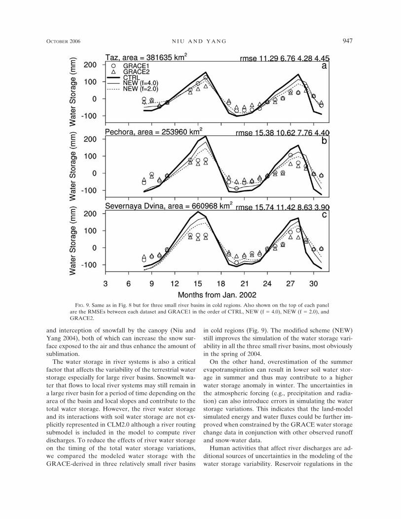
The water storage in river systems is also a criticalfactor that affects the variability of the terrestrial waterstorage especially for large river basins. Snowmelt wa-ter that flows to local river systems may still remain ina large river basin for a period of time depending on thearea of the basin and local slopes and contribute to thetotal water storage. However, the river water storageand its interactions with soil water storage are not ex-plicitly represented in CLM2.0 although a river routingsubmodel is included in the model to compute riverdischarges. To reduce the effects of river water storageon the timing of the total water storage variations,we compared the modeled water storage with theGRACE-derived in three relatively small river basins

in cold regions (Fig. 9). The modified scheme (NEW)still improves the simulation of the water storage vari-ability in all the three small river basins, most obviouslyin the spring of 2004.

On the other hand, overestimation of the summerevapotranspiration can result in lower soil water stor-age in summer and thus may contribute to a higherwater storage anomaly in winter. The uncertainties inthe atmospheric forcing (e.g., precipitation and radia-tion) can also introduce errors in simulating the waterstorage variations. This indicates that the land-modelsimulated energy and water fluxes could be further im-proved when constrained by the GRACE water storagechange data in conjunction with other observed runoffand snow-water data.

Human activities that affect river discharges are ad-ditional sources of uncertainties in the modeling of thewater storage variability. Reservoir regulations in the

FIG. 9. Same as in Fig. 8 but for three small river basins in cold regions. Also shown on the top of each panelare the RMSEs between each dataset and GRACE1 in the order of CTRL, NEW (f � 4.0), NEW (f � 2.0), andGRACE2.


Yenisei River basin (Yang et al. 2004) and the LenaRiver basin (Ye et al. 2003) have significantly alteredthe river discharges by retaining water in summer andreleasing water in winter, thereby resulting in less run-off in summer and more runoff in winter. An additionalexperiment that produces less runoff in summer andmore runoff in winter by adjusting the runoff decayfactor [ f in Eqs. (B2) and (B3)] from 4.0 to 2.0 m�1

further improves the simulation (Figs. 8 and 9).

5. Tests of two alternative hydraulic properties

The proposed frozen soil scheme as described in pre-vious sections consists of three parts that are closelyrelated to each other. First, the amount of (super-cooled) liquid water is governed by the freezing-pointdepression equation. This part is necessary in that itdefines an upper limit at which soil water can remain inliquid form for temperatures below the freezing pointof pure water. Without this part, as is the case inCLM2.0/SIMTOP, soil water tends to become icewhenever the soil temperature is below the freezingpoint of pure water. Second, the soil hydraulic proper-ties are defined as a function of a ratio of total (liquidand ice) soil moisture to soil porosity. The reason to usethe total liquid and ice soil moisture here is tied inti-mately to the next part. Third, the hydraulic conductiv-ity is multiplied by the fractional permeable area, whichintegrates the effects of soil macropores and (super-cooled) liquid water on infiltration at the soil surfaceand percolation between the soil layers. All these threeparts are integral to the whole framework, which isshown to greatly improve the runoff simulation by in-creasing the infiltration capacity of frozen soil. Thisnotwithstanding, it is of interest to see whether equallygood simulations can result if the second and third partsof the new frozen soil scheme are represented differ-ently.

Indeed, there are two other major forms of param-eterizations of soil hydraulic properties that have ap-peared in the literature. In the first form, the soil hy-draulic properties are expressed as a function of a ratioof (supercooled) liquid water only to soil porosity(Flerchinger and Saxton 1989, hereafter referred to asFS; Cox et al. 1999; Hansson et al. 2004):

k � ksat��liq��sat�2b�3, �13�

� � �sat��liq��sat��b. �14�

In the second form, the soil hydraulic properties areexpressed as a function of a ratio of (supercooled) liq-uid water to effective soil porosity, defined as soil po-rosity minus ice content (Zhao and Gray 1997, hereaf-ter ZG):

k � 10�E�iceksat� �liq

�sat � �ice�2b�3

, �15�

� � �sat� �liq

�sat � �ice��b

, �16�

where E is the impedance factor accounting for theeffect of ice on soil permeability, and E � 7.0.

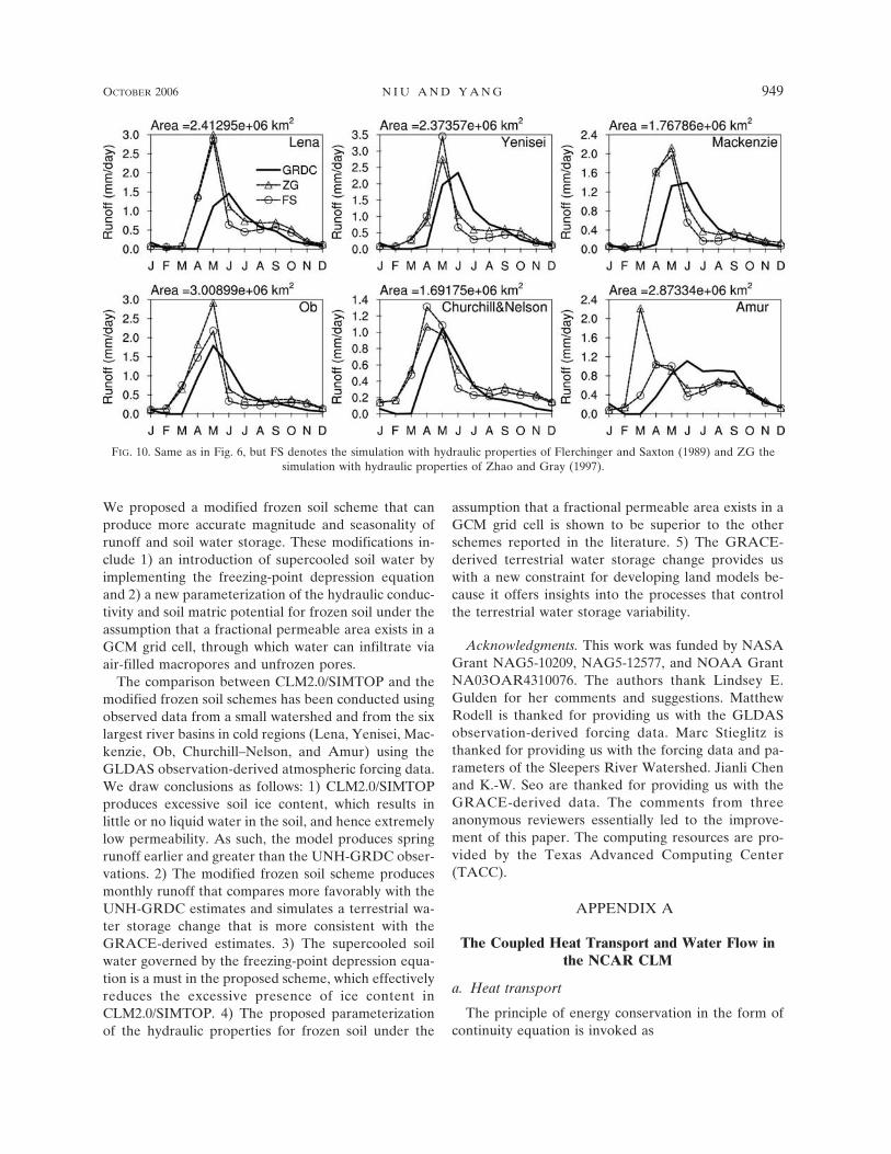
Both forms do not employ the concept of the frac-tional permeable area. To evaluate the hydrologic im-pacts of using the above two forms in CLM2.0/SIMTOP,we conducted two separate runs. In the experiment totest the FS scheme, we replaced Eqs. (9) and (10) withEqs. (13) and (14), respectively. In the experiment totest the ZG scheme, we replaced Eqs. (9) and (10) withEqs. (15) and (16), respectively. Both schemes produceearlier- and higher-than-observed runoff in all the sixriver basins (Fig. 10). Additionally, both schemes pro-duce a much smaller infiltration capacity in the soil thanthe proposed scheme as described in section 2b. Weconclude that replacing the second and third parts inthe proposed frozen soil scheme with either FS or ZGfails to produce realistic simulations of runoff. The ZGscheme with a smaller impedance factor (e.g., E � 2.0)did a good job (figures not shown). However, the im-pedance factor is smaller than the value reported inliterature by a factor of 3.5–5.0 (Takata 2002).

These tests have demonstrated that the second andthird parts in the proposed scheme are superior to ei-ther the FS or ZG schemes. In the proposed scheme,hydraulic properties are expressed by the total soil wa-ter content, thereby greatly increasing the infiltrationcapacity of the frozen soil. Furthermore, given a frozenground as large as a GCM grid cell, it is not uncommonto see the presence of macropores and/or snowmelt wa-ter flowing from impermeable to permeable areas. Assuch, it appears to be reasonable to assume a fraction ofthe frozen ground that is permeable. The fractional per-meable area is parameterized such that it allows theinfiltration capacity of the frozen ground to decreasemore slowly than Eqs. (13) or (15) do.

6. Conclusions

Soil hydrologic and thermal properties are altereddramatically by the presence of soil ice. This studyshows how a land surface model that explicitly repre-sents the hydrologic effects of soil ice can improve thesimulations of runoff and soil water storages by em-ploying CLM2.0/SIMTOP. A frozen soil scheme, inwhich the soil ice content is solely determined by theavailable energy, as in CLM2.0/SIMTOP, should bemodified to take into consideration the hydrologic ef-fects of the supercooled soil water and relax the depen-dence of hydraulic properties on the soil ice content.


We proposed a modified frozen soil scheme that canproduce more accurate magnitude and seasonality ofrunoff and soil water storage. These modifications in-clude 1) an introduction of supercooled soil water byimplementing the freezing-point depression equationand 2) a new parameterization of the hydraulic conduc-tivity and soil matric potential for frozen soil under theassumption that a fractional permeable area exists in aGCM grid cell, through which water can infiltrate viaair-filled macropores and unfrozen pores.

The comparison between CLM2.0/SIMTOP and themodified frozen soil schemes has been conducted usingobserved data from a small watershed and from the sixlargest river basins in cold regions (Lena, Yenisei, Mac-kenzie, Ob, Churchill–Nelson, and Amur) using theGLDAS observation-derived atmospheric forcing data.We draw conclusions as follows: 1) CLM2.0/SIMTOPproduces excessive soil ice content, which results inlittle or no liquid water in the soil, and hence extremelylow permeability. As such, the model produces springrunoff earlier and greater than the UNH-GRDC obser-vations. 2) The modified frozen soil scheme producesmonthly runoff that compares more favorably with theUNH-GRDC estimates and simulates a terrestrial wa-ter storage change that is more consistent with theGRACE-derived estimates. 3) The supercooled soilwater governed by the freezing-point depression equa-tion is a must in the proposed scheme, which effectivelyreduces the excessive presence of ice content inCLM2.0/SIMTOP. 4) The proposed parameterizationof the hydraulic properties for frozen soil under the

assumption that a fractional permeable area exists in aGCM grid cell is shown to be superior to the otherschemes reported in the literature. 5) The GRACE-derived terrestrial water storage change provides uswith a new constraint for developing land models be-cause it offers insights into the processes that controlthe terrestrial water storage variability.

Acknowledgments. This work was funded by NASAGrant NAG5-10209, NAG5-12577, and NOAA GrantNA03OAR4310076. The authors thank Lindsey E.Gulden for her comments and suggestions. MatthewRodell is thanked for providing us with the GLDASobservation-derived forcing data. Marc Stieglitz isthanked for providing us with the forcing data and pa-rameters of the Sleepers River Watershed. Jianli Chenand K.-W. Seo are thanked for providing us with theGRACE-derived data. The comments from threeanonymous reviewers essentially led to the improve-ment of this paper. The computing resources are pro-vided by the Texas Advanced Computing Center(TACC).

APPENDIX A

The Coupled Heat Transport and Water Flow inthe NCAR CLM

a. Heat transport

The principle of energy conservation in the form ofcontinuity equation is invoked as

FIG. 10. Same as in Fig. 6, but FS denotes the simulation with hydraulic properties of Flerchinger and Saxton (1989) and ZG thesimulation with hydraulic properties of Zhao and Gray (1997).


C�T

�t�

�

�z ��T

�z� � �iceLf

��ice

�t, �A1�

where t and z are time and height above some datum inthe soil column (positive upward), repectively, and Cand � are the volumetric heat capacity and the thermalconductivity, respectively. The second term on theright-hand side is the rate of energy released fromfreezing or consumed by melting. Here �ice (917 kgm�3) and �ice are the density and partial volume of icecontent, respectively, and Lf is the latent heat of fusion(0.3336 106 J kg�3).

The volumetric heat capacity C (J m�3 K�1) is fromde Vries (1963) and depends on the volumetric heatcapacities of the soil matrix, Csoi, liquid water, Cliq, andice constituents, Cice:

C � Csoi�1 � �sat� � Cice�ice � Cliq�liq, �A2�

where �sat is the porosity. �liq is the partial volume ofliquid water.

Soil thermal conductivity � (W m�1 K�1) is fromFarouki (1981):

� � Ke�sat � �1 � Ke��dry, �A3�

where Ke is the Kersten number and �dry is the thermalconductivity of dry soil as a function of soil bulk density(see Oleson et al. 2004 for detail). The saturated ther-mal conductivity � (W m�1 K�1) depends on the ther-mal conductivities of the soil matrix, �soi, liquid water,�liq, and ice constituents, �ice:

�sat � �soi�1��sat��liq

�liq�ice�ice, �A4�

where the thermal conductivity of soil matrix varieswith the sand and clay content, and �liq � 0.59W m�1

K�1 and �ice � 2.29 W m�1 K�1.

b. Water transport

The conservation of liquid water for one-dimensionalvertical water flow in the soil is expressed as

��liq

�t� �

�q

�z� E � Rfm, �A5�

where q is the soil water flux (mm s�1), E is the evapo-transpiration rate, and Rfm is the melting or freezingrate.

The soil water flux q is described by Darcy’s law:

q � �k�� z�

�z, �A6�

where k is the hydraulic conductivity (mm s�1), � is thesoil matric potential (mm), and z is the depth from thesoil surface.

The hydraulic conductivity and the soil matric poten-tial vary with volumetric soil water and soil texturebased on the work of Clapp and Hornberger (1978) andCosby et al. (1984). In frozen soil, the hydraulic con-ductivity and soil matric potential vary with the partialvolume of liquid water:

k � �ksat��liq��sat�2b�3

0

�e 0.05

�e 0.05, �A7�

� � ��sat��liq��sat�

�b

103Lf �T � Tfrz�

gT

T � Tfrz

T � Tfrz

, �A8�

where ksat (mm s�1) and �sat (mm) are the saturatedhydraulic conductivity and the saturated soil matric po-tential depending on the soil texture, b is referred to asthe Clapp–Hornburger parameter, and g is the gravita-tional acceleration (m s�2).

The conservation of the partial volume of ice is

��ice

�t� Rfm, �A9�

where Rfm � Hfm/(�iceLf z), where Hfm (W m�2) is theenergy for freezing (positive) or melting (negative).The ice content for the next time step is

�ice

N � 1 � min��N, �iceN � Rfm�t�, �A10�

where �N � �ice � �liq is the total volumetric soil watercontent.

The energy for freezing or melting (Hfm) is assessedfrom the energy excess or deficit needed to change soiltemperature to freezing point Tfrz:

Hfm � C�zTfrz � TN�1

�t, �A11�

where TN�1 is the layer temperature resulting from allthe other processes except for phase change, and zand t are the layer depth and time step. In freezingphase (when �liq 0 and TN�1 � Tfrz, where Tfrz �273.16 K), Hfm is limited by the latent energy releasedfrom freezing all the liquid water in a layer within atime step, that is, Lf�liq�liq z/ t (W m�2), where �liq isthe liquid water density (1000 kg m�3). In meltingphase (when �ice 0 and TN�1 Tfrz), Hfm is limited bythe latent energy consumed for melting all the ice in alayer within a time step, Lf�ice�ice z/ t (W m�2). Theresidual energy that may not be consumed by meltingor released from freezing is used to warm or cool thesoil layer.


APPENDIX B

A Simple TOPMODEL-Based Runoff Scheme

The runoff scheme used in the simulations presentedhere is a simple TOPMODEL-based runoff model (Niuet al. 2005). In SIMTOP, the saturated hydraulic con-ductivity Ksat can either be defined as a function of soiltexture as in climate models or decay exponentiallywith soil depth as in TOPMODEL applications. In thisstudy, Ksat is defined as a function of soil texture, be-cause it is commonly defined in this way in the landmodel community.

The surface runoff,

Rs � FsatQwat � �1 � Fsat� max�0, �Qwat � Imax��, �B1�

where Qwat is the input of water (sum of rainfall, dew-fall, and snowmelt) incident on the soil surface, and Imax

is the soil infiltration capacity dependent on soil textureand moisture conditions. The saturated fraction, Fsat, isparameterized as

Fsat � �Fmaxe�0.5fz�

1.0

�e 0.05

�e 0.05, �B2�

where Fmax is the potential or maximum saturated frac-tion for a grid cell, and Fmax is defined as the cumulativedistribution function (CDF) of the topographic indexwhen the grid-mean water table depth is zero, that is,the percent of the pixels with topographic index largerthan its grid-cell or catchment-averaged value. Here�e � �sat � �ice is the effective porosity. The decayfactor, f, can be determined through sensitivity analysisor calibration against the hydrograph recession curve;z� is the grid-cell–mean water table depth.

The subsurface runoff is parameterized as

Rsb � Rsb, maxe�fz�, �B3�

where Rsb, max is the maximum subsurface runoff whenthe grid-cell averaged water table depth is zero. HereRsb,max � 1.0 10�4 mm s�1.

REFERENCES

Aagaard, K., and E. C. Carmack, 1989: The role of sea ice andother fresh-water in the arctic circulation. J. Geophys. Res.,94 (C10), 14 485–14 498.

Barry, R. G., and M. C. Serreze, 2000: Atmospheric componentsof the Arctic Ocean freshwater balance and their interannualvariability. The Freshwater Budget of the Arctic Ocean, E. L.Lewis et al., Eds., Springer, 45–56.

Bayard, D., M. Stahli, A. Parriaux, and H. Fluhler, 2005: Theinfluence of seasonally frozen soil on snowmelt runoff at twoAlpine sites in southern Switzerland. J. Hydrol., 209, 66–84.

Bengtsson, L., P. Seuna, A. Lepisto, and R. Saxena, 1992: Particle

movement of melt water in a subdrained agricultural basin. J.Hydrol., 135, 383–398.

Bonan, G. B., K. W. Oleson, M. Vertenstein, S. Levis, X. Zeng, Y.Dai, R. E. Dickinson, and Z.-L. Yang, 2002: The land surfaceclimatology of the Community Land Model coupled to theNCAR Community Climate Model. J. Climate, 15, 3123–3149.

Broecker, W. S., 1997: Thermohaline circulation, the Achilles heelof our climate system: Will man-made CO2 upset the currentbalance? Science, 278, 1582–1588.

Chen, J. L., M. Rodell, C. R. Wilson, J. S. Famiglietti, 2005: Lowdegree spherical harmonic influences on Gravity Recoveryand Climate Experiment (GRACE) water storage estimates.Geophys. Res. Lett., 32, L14405, doi:10.1029/2005GL022964.

Cherkauer, K., and D. P. Lettenmaier, 2003: Simulation of spatialvaribility in snow and frozen soil. J. Geophys. Res., 108, 8858,doi:10.1029/2003JD003575.

Clapp, R. B., and G. M. Hornberger, 1978: Empirical equationsfor some soil hydraulic properties. Water Resour. Res., 14,601–604.

Cosby, B. J., G. M. Hornberger, R. B. Clapp, and T. R. Ginn,1984: A statistical exploration of the relationships of soilmoisture characteristics to the physical properties of soils.Water Resour. Res., 20, 682–690.

Cox, P. M., R. A. Betts, C. B. Bunton, R. L. H. Essery, P. R.Rowntree, and J. Smith, 1999: The impact of new land surfacephysics on the GCM simulation of climate and climate sen-sitivity. Climate Dyn., 15, 183–203.

de Vries, D. A., 1963: Thermal properties of soils. Physics of thePlant Environment, W. R. van Wijk, Ed., North-Holland,210–235.

Dunne, T., and R. D. Black, 1971: Runoff processes during snow-melt. Water Resour. Res., 7, 1160–1172.

Farouki, O. T., 1981: The thermal properties of soils in cold re-gions. Cold Regions Sci. Technol., 5, 67–75.

Fekete, B. M., C. J. Vorosmarty, and W. Grabs, cited 2000: Globalcomposite runoff fields based on observed discharge andsimulated water balance. [Available online at http://www.grdc.sr.unh.edu/html/paper/ReportUS.pdf.]

Flerchinger, G. N., and K. E. Saxton, 1989: Simultaneous heat andwater model of a freezing snow–residue–soil system. I.Theory and development. Trans. ASAE, 32, 565–571.

Flury, M., H. Flühler, W. A. Jury, and J. Leuenberger, 1994: Sus-ceptibility of soils to preferential flow of water: A field study.Water Resour. Res., 30, 1945–1954.

Foster, D. J., and R. D. Davy, 1988: Global snow depth climatol-ogy. Tech. Note USAFETAC/TN-88/006, Scott Air ForceBase, IL, 48 pp.

Fuchs, M., G. S. Campbell, and R. I. Papendick, 1978: An analysisof sensible and latent heat flow in a partially frozen unsatu-rated soil. Soil Sci. Soc. Amer. J., 42, 379–385.

Hansson, K., J. Simunek, M. Mizoguchi, L.-C. Lundin, and M. T.van Genuchten, 2004: Water flow and heat transport in fro-zen soil: Numerical solution and freeze-thaw applications.Vadose Zone J., 3, 693–704.

Kane, D. L., and J. Stein, 1983: Water movement into seasonallyfrozen soils. Water Resour. Res., 19, 1547–1557.

Koren, V., 1980: Modeling of processes of river runoff formationin the forest zone of European USSR. Meteorology and Hy-drology, No. 10, Allerton Press, 78–85.

——, J. Schaake, K. Mitchell, Q.-Y. Duan, F. Chen, and J. M.Baker, 1999: A parameterization of snowpack and frozen


ground intended for NCEP weather and climate models. J.Geophys. Res., 104 (D16), 19 569–19 585.

Lindstrom, G., K. Bishop, and M. O. Lofvenius, 2002: Soil frostand runoff at Svartberget, northern Sweden—Measurementsand model analysis. Hydrol. Processes, 16, 3379–3392.

Luo, L. F., and Coauthors, 2003: Effects of frozen soil on soiltemperature, spring infiltration, and runoff: Results from thePILPS 2(d) experiment at Valdai, Russia. J. Hydrometeor., 4,334–351.

McDonald, R. W., E. C. Cramack, F. A. Mclaughlin, K. K.Falkner, and J. H. Swift, 1999: Connections among ice, runoffand atmospheric forcing in Beaufort Sea. Geophys. Res. Lett.,26, 2223–2226.

Niu, G.-Y., and Z.-L. Yang, 2004: The effects of canopy processeson snow surface energy and mass balances. J. Geophys. Res.,109, D23111, doi:10.1029/2004JD004884.

——, ——, R. E. Dickinson, and L. E. Gulden, 2005: A simpleTOPMODEL-based runoff parameterization for use inGCMs. J. Geophys. Res., 110, D21106, doi:10.1029/2005JD006111.

Nyberg, L., M. Stahli, P. E. Mellander, and K. Bishop, 2001: Soilfrost effects on soil water and runoff dynamics along a borealforest transact: 1. Field investigations. Hydrol. Processes, 15,909–926.

Oleson, K. W., and Coauthors, 2004: Technical description of theCommunity Land Model (CLM). Tech. Note NCAR/TN-461�STR, 174 pp. [Available online at www.cgd.ucar.edu/tss/clm/distribution/clm3.0/index.html.]

Peterson, B. J., R. M. Holmes, J. W. McClelland, C. J. Voros-marty, R. B. Lammers, A. I. Shiklomanov, I. A. Shiklo-manov, and S. Rahmstorf, 2002: Increasing river discharge tothe Arctic Ocean. Science, 298, 2171–2173.

Pitman, A. J., A. G. Slater, C. E. Desborough, and M. Zhao, 1999:Uncertainty in the simulation due to the parameterization offrozen soil moisture using the Global Soil Wetness Projectmethodology. J. Geophys. Res., 104 (D14), 16 879–16 888.

Poutou, E., G. Krinner, C. Genthon, and N. de Noblet-Ducoudre,2004: Role of soil freezing in future boreal climate change.Climate Dyn., 23, 621–639.

Robock, A., K. Y. Vinnikov, C. A. Schlosser, N. A. Speranskaya,and Y. Xue, 1995: Use of midlatitude soil moisture and me-teorological observations to validate soil moisture simula-tions with biosphere and bucket models. J. Climate, 8, 15–35.

Rodell, M., and Coauthors, 2004a: The global land data assimila-tion system. Bull. Amer. Meteor. Soc., 85, 381–394.

——, J. S. Femiglietti, J. L. Chen, S. I. Seneviratne, P. Viterbo,and S. Holl, 2004b: Basin scale estimates of evapotranspira-tion using GRACE and other observations. Geophys. Res.Lett., 31, L20504, doi:10.1029/2004GL020873.

Sellers, P. J., and Coauthors, 1996: A revised land surface param-eterization (SiB2) for atmospheric GCMs. Part I: Model for-mulation. J. Climate, 9, 676–705.

Seo, K. W., and C. R. Wilson, 2005: Simulated estimation of hy-drological loads from GRACE. J. Geod., 78, 442–456.

Shanley, J. B., and A. Chalmers, 1999: The effect of frozen soil onsnowmelt runoff at Sleepers River, Vermont. Hydrol. Pro-cesses, 13, 1843–1857.

Spaans, E. J. A., and J. M. Baker, 1996: The soil freezing charac-teristic: Its measurement and similarity to the soil moisturecharacteristic. Soil Sci. Soc. Amer. J., 60, 13–19.

Stadler, D., H. Wunderli, A. Auckenthaler, and H. Fluhler, 1996:Measurements of frost-induced snowmelt runoff in a forestsoil. Hydrol. Processes, 10, 1293–1304.

——, H. Flühler, and P.-E. Jansson, 1997: Modelling vertical andlateral water flow in frozen and sloped forest soil plots. ColdReg. Sci. Technol., 26, 181–194.

——, M. Stähli, P. Aeby, and H. Flühler, 2000: Dye tracing andimage analysis for quantifying water infiltration into frozensoils. Soil Sci. Soc. Amer. J., 64, 505–516.

Stähli, M., P.-E. Jansson, and L.-C. Lundin, 1999: Soil moistureredistribution and infiltration in frozen sandy soils. WaterResour. Res., 35, 95–103.

——, L. Nyberg, P.-E. Mellander, P.-E. Jansson, and K. H.Bishop, 2001: Soil frost effects on soil water and runoff dy-namics along a boreal forest transact: 2. Simulations. Hydrol.Processes, 15, 927–941.

——, D. Bayard, H. Wydler, and H. Flühler, 2004: Snowmelt in-filtration into alpine soils visualized by dye tracer technique.Arct. Antarct. Alp. Res., 36, 128–135.

Stieglitz, M., D. Rind, J. Famiglietti, and C. Rosenzweig, 1997: Anefficient approach to modeling the topographic control ofsurface hydrology for regional and global modeling. J. Cli-mate, 10, 118–137.

Su, F. G., J. C. Adam, L. C. Bowling, and D. P. Lettenmaier, 2005:Streamflow simulations of the terrestrial Arctic domain. J.Geophys. Res., 110, D08112, doi:10.1029/2004JD005518.

Takata, K., 2002: Sensitivity of land surface processes to frozensoil permeability and surface water storage. Hydrol. Pro-cesses, 16, 2155–2172.

Tapley, B. D., and Coauthors, 2004: GRACE measurements ofmass variability in the earth system. Science, 305, 503–505.

Wahr, J., S. Swenson, V. Zlotnicki, and I. Velicogna, 2004: Time-variable gravity from GRACE: First results. Geophys. Res.Lett., 31, L11501, doi:10.1029/2004GL019779.

Warrach, K., M. Stieglitz, H. T. Mengelkamp, and E. Raschke,2002: Advantages of a topographically controlled runoffsimulation in a soil–vegetation–atmosphere transfer model. J.Hydrometeor., 3, 131–148.

Xue, Y., P. J. Sellers, J. L. Kinter, and J. Shukla, 1991: A simpliedbiosphere model for global climate studies. J. Climate, 4, 345–364.

——, F. J. Zeng, and C. A. Schlosser, 1996: SSiB and its sensitivityto soil properties: A case study using HAPEX-mobilhy data.Global Planet. Change, 13, 183–194.

Yang, D., B. Ye, and D. L. Kane, 2004: Streamflow changes overSiberian Yenisei River basin. J. Hydrol., 296, 59–80.

Yang, Z.-L., and R. E. Dickinson, 1996: Description of the Bio-sphere–Atmosphere Transfer Scheme (BATS) for the soilmoisture workshop and evaluation of its performance. Glob-al Planet. Change, 13, 117–134.

Ye, B., D. Yang, and D. L. Kane, 2003: Changes in Lena Riverstreamflow hydrology: Human impacts versus natural varia-tions. Water Resour. Res., 39, 1200, doi:10.1029/2003WR001991.

Zhang, T., R. G. Barry, K. Knowles, J. A. Heginbottom, and J.Brown, 1999: Statistics and characteristics of permafrost andground ice distribution in the Northern Hemisphere. Pol.Geogr., 23 (2), 147–169.

Zhao, L., and D. M. Gray, 1997: A parametric expression forestimating infiltration into frozen soils. Hydrol. Processes, 11,1761–1775.


effects of frozen soil on snowmelt runoff and soil water ...effects of frozen soil on snowmelt...

Documents