is the use of brewery spent grain in …sure.sunderland.ac.uk/5187/1/orurufinal_copy_in_pdf.pdf ·...
TRANSCRIPT

i
IS THE USE of BREWERY SPENT GRAIN IN
BIOREMEDIATION OF DIESEL CONTAMINATED SOIL
SUSTAINABLE?
JOHNSON AJORITSEDEBI ORURU
A thesis submitted in partial fulfilment of the requirements of the University of
Sunderland for the Degree of Doctor of Philosophy
April 2014

ii
DECLARATION
I wish to say that no component of the work referred in this report has been
submitted in support of any application for another qualification for this or any other
institutions of learning

iii
ACKNOWLEGMENTS
Firstly, my immense and treasured thank goes to my Father, the Almighty God
through Jesus Christ my Lord, without whom I am nothing.
My profound and sincere thank goes to my excellent supervisors Dr. Monica Price
and Dr. Keith Thomas. I am particularly thanking Dr. Monica Price whose meticulous
supervisory skills and encouragement helped me greatly in bringing this work to a
good conclusion.
I would like to thank all member of the laboratory staffs of the University of
Sunderland especially Mr Arun Mistry who give advice along the way in carrying the
laboratory work.
My deepest gratitude also goes to my beloved wife Mrs.Carol Oruru whose affection,
encouragement, dedication and prayer sustained me through this trying and difficult
period of writing this thesis. I also owe so much to Tuoyor and Tosan and Toju whose
presence and affection were of great encouragement to me.
Finally, my immense appreciation goes to the member of MFN Newcastle branch for
their prayer and supplication during my trying and difficult time and would like to say
big thanks to Richard Grant for providing the information for the economic and
environmental costs used in the study and providing useful advice.
iv
Abstract
Remediation of contaminated land needs to be carried out using methods that are
both cost effective and minimise environmental pollution. However, the remediation
option currently chosen by practitioners is often based upon limited economic
information with the true environmental costs not being considered. This can result in
the least sustainable option being chosen.
This study has developed a methodology to evaluate the sustainability, in terms of
economic and environmental costs, for a range of treatments available for the
remediation of diesel contaminated land, including bioremediation (with and without
the addition of brewery spent grain), disposal to landfill and thermal treatment.
Initial laboratory investigations indicated that the use of brewery spent grain
decreased the time taken for the clean-up of soil contaminated with diesel,
suggesting that bioremediation augmented by the addition of this organic material
was a viable option. A costing model was then developed that included all of the
costs associated with the remediation options chosen. This included both direct and
indirect costs. The results show that considering the indirect costs of remediation
such as costs associated with delayed development the land, make bioremediation
in this study an economically feasible option.
Finally environmental costs were considered with a focus on the release of carbon
dioxide a known greenhouse gas. Respirometry was used to determine the volume
of carbon dioxide released during the bioremediation process. This information was
then combined with data collected from a range of other sources and the impact of
the chosen remediation options on atmospheric greenhouse gas release was
evaluated. Other environmental impacts were also determined including land and
water pollution. The results indicate that bioremediation with brewery spent grain has
one of the lowest environmental costs and showed that emission from pollutants
such as NOx, PM1.0, PM2.5, NH3 and SO2 could contribute to the limit values in the
area covered by remediation work.
The model developed in this study has indicated that the use of bioremediation with
and without the use of brewery spent grain is a sustainable remediation option
providing both direct and indirect economic costs are included. The results have
indicated that, the strategy of using brewery spent grain to augment bioremediation

v
process promotes the re-use of by-product material, reduces waste and conserve
resources. There is a need for the remediation industry to adopt similar models in
order that decisions made, as to the remediation option chosen, are based upon
accurate costings of their sustainability.

vi
TABLE OF CONTENTS
DECLARATION......................................................................... ii
ACKNOWLEDGEMENTS.......................................................... iii
ABSTRACT................................................................................ iv
LIST OF TABLES IN TEXT..................................................... xi
LIST OF FIGURES IN TEXT..................................................... xvi
1. Introduction................................................................ 1
1.1 Introduction................................................................................ 1
1.2 Background to the research....................................................... 2
1.3
1.4
Aims and Objectives..................................................................
Structure of the thesis……………………………………………..
3
4
2. Literature Review....................................................... 6
2.1 Introduction................................................................................ 6
2.2 Remediation of Contaminated Soils.......................................... 7
2.3 Physicochemical Methods for Hydrocarbon Remediation…...... 8
2.4 Soil vapor extraction.................................................................. 10
2.5 Thermal desorption.................................................................... 14
2.6 Biological Methods for Hydrocarbon Remediation..................... 17
2.6.1 Natural Attenuation................................................................ 20
2.6.2 Bio-augmentation................................................................... 20
2.6.3 Bio-stimulation........................................................................ 21
2.6.4 Factors Affecting Bioremediation............................................ 22
2.6.5 Disadvantages of Bioremediation.............................................. 25
2.7 Monitoring and Measurement of Bioremediation....................... 26
2.7.1 Biological techniques.............................................................. 30
2.7.2 Chemical Analysis.................................................................. 33
2.7.3 Gas chromatography (GC)……………………………………... 34
2.8 Waste management................................................................... 35
2.9 Classification of waste............................................................... 38
2.9.1 Brewery spent grain................................................................... 39
2.9.2 BSG as a Bio-waste................................................................... 42
2.10 Sustainability: what it is.............................................................. 42
2.10.1 Application of sustainability to remediation of contaminated

vii
land............................................................................................ 44
2.10.2
2.10.3
2.10.4
2.10.5
2.11
3.
3.1
3.1.1
3.2
3.3
3.4
3.4.1
3.4.2
3.5
3.5.1
3.5.2
3.6
3.7
3.7.1
3.7.2
3.7.3
3.7.4
3.8
3.9
4
4.1
4.1.1
4.2
4.2.1
4.2.2
4.3
4.3.1
4.3.2
Measurement of sustainable indicators in the UK.....................
Appraisal of the SuRF and Defra guidelines…………………….
Sensitivity analysis…………………………………………………
Setting the boundaries of a sustainability assessment…………
Conclusions…………………………………………………………
Materials and methods…………….…………………………….
Introduction………………………………………………………….
Laboratory Work……………………………………………………
Soil preparation and experimental design……………………….
Experimental design and maintenance…………………………..
Microbiological methods…………………………………………...
Culture Media……………………………………………………….
Formulation of media preparation which was used in the
study…………………………………………………………………
Analytical Methods…………………………………………………
Diesel Extraction for Gas Chromatography……………………..
Chemical analysis of hydrocarbons………………………………
Statistical Analysis used in the study……….……………………
Evaluation of Methods and Development of Techniques………
Introduction………………………………………………………….
Soil spiking………………………………………………………...
Percentage recovery……………………………………………….
Representation of the effect of concentration on% recovery….
Determination of water holding capacity (WHC)………………..
Conclusions………………………………………………………..
Laboratory scale evaluation of bioremediation of brewery
spent grain…………………………………………………………..
Introduction………………………………………………………….
Review of bioremediation technique
Methods……………………………………………………………..
Monitoring and maintaining the experiment……………………..
Microbial analysis..……………………………………………….
Results of Experiment (a)………………………………………….
TPH Analysis………………………………………………………..
Statistical results of TPH…………………………………………..
45
52
54
55
55
57
57
58
58
59
60
60
61
63
63
63
65
65
65
66
69
70
71
72
73
73
73
74
76
76
76
77
78

viii
4.3.3
4.3.3.1
4.3.4
4.4
4.4.1
4.4.2
4.5
4.5.1
4.5.2
4.5.3
4.5.3.1
4.5.3.2
4.5.4
4.6
4.6.1
4.6.2
4.6.3
4.7
5.
5.1
5.1.1
5.1.2
5.1.3
5.2
5.2.1
5.3
5.3.1
5.3.1.1
5.3.1.2
5.3.1.3
5.3.1.4
5.3.1.5
5.3.2
5.3.2.1
5.3.2.2
Microbial analysis…………………………………………………..
Statistical results of microbial counts…………………………….
pH and temperature analysis……………………………………..
Methods……………………………………………………………..
Methods of experiment (b)………………...………………………
Monitoring and maintaining the experiment……………………..
Results of Experiment (b)………………………………………….
TPH analysis………………………………………………………..
Statistical analysis………………………………………………….
Microbial analysis…………………………………………………..
CFU Enumeration…………………………………………………..
Statistical analysis of microbial populations……………………..
pH and temperature analysis……………………………………..
Discussion…………………………………………………………..
Microbial analysis…………………………………………………..
pH values and temperature……………………………………….
TPH (Total Petroleum Hydrocarbon)……………………………..
Conclusions…………………………………………………………
Is the use of brewery spent grain cost-effective?................
Introduction………………………………………………………….
The use of brewery spent grain to remediate diesel contaminated
site……………….………………………………..
Discussions with the remediation expert and case study site…
Developing the case study site……………………………………
. Methods……………………………………………………………
Justification for the values costs adopted…………………….
Results………………………………………………………………
Direct Costs……………………………………………………...
Bioremediation with and without Brewery Spent Grain……….
Natural Attenuation………………………………………………..
Disposal and re-filling the earth…………………………………..
Soil vapour extraction………………………………………….....
Thermal desorption………………………………………………...
Indirect Costs……………………………………………………….
Bioremediation with and without Brewery Spent Grain………...
Natural Attenuation…………………………………………………
82
84
88
89
89
91
91
92
97
100
100
102
106
107
108
110
112
115
117
117
117
118
120
124
127
137
139
139
140
140
141
141
141
141
142
ix
5.3.2.3
5.3.2.4
5.3.2.5
5.4
5.4.1
5.5
5.6
5.6.1
5.7
6.
6.1
6.1.1
6.2
6.2.1
6.2.2
6.3
6.3.1
6.4
6.4.1
6.4.2
6.4.3
6.4.4
6.4.5
6.4.6
6.5
6.5.1
6.5.2
6.5.3
6.5.4
6.5.5
6.6
6.6.1
6.6.2
6.6.3
Disposal to Landfill…………………………………………………
Soil vapour Extraction……………………………………………...
Thermal desorption………………………………………………...
Sensitivity Analysis…………………………………………………
Economic costs associated with varying soil quantities………..
Discussions…………………………………………………………
Sensitivity Analysis………………………………….……………..
Sensitivity analysis for comparing the costs of 40,000, 10,000 and
4,000 tonnes for six different remediation options…………
Conclusions…………………………………………………………
Environmental impact of different remediation options….
Introduction………………………………………………………….
Environmental impacts of land contamination…………………
Methods……………………………………………………………..
Practical methods…………………………………………………..
Measuring of soil respiration and determination of CO2…………..
Data collection………………………………………………………
Emission factors and their Justification…………………………..
Results……………………………………………………………....
Air pollution………………………………………………………….
Bioremediation emissions………………………………………...
Natural attenuation processes (CO2)…………………………….
Landfill disposal option (CO2)……………………………………..
Soil vapours extraction method (CO2)……………………………
Thermal desorption………………………………………………...
Impacts of remediation activities on water and land……….…...
Bioremediation with and without brewery spent grain on land and
water pollution…………………………….…………………...
Natural attenuation effects on land water pollution……………
Landfill disposal effects on land water pollution……………….
Soil vapour extraction effect on land and water pollution.…......
Thermal desorption effect on land and water pollution…..….....
Discussions…………………………………………………...…….
Process and activities emissions……………………...………….
Process emissions from bioremediation technique….…………
Process emissions from natural attenuation and landfill disposal
142
142
143
143
143
145
150
150
153
154
154
154
156
157
159
165
167
171
171
172
177
178
185
187
189
191
192
193
193
194
194
195
195
x
6.6.4
6.7
6.8
6.9
6.10
6.11
7.
7.1
7.2
7.3
7.4
7.5
8.
8.1
8.2
9.
option techniques…………………….………………….
Process emissions from soil vapour and thermal desorption
technique……………………………..……………………………...Activ
ities emissions from transportation, use of energy and other
remediation activities………………………………………..
Other conventional air pollution……...…………………………...
Water impacts …...…………………………………………………
Land impacts……………………..…………………………………
Conclusions………………………………………………………..
Discussions…………….………………………………………….
Introduction………………………………………………………….
Does the addition of brewery spent grain improve the
bioremediation of hydrocarbon contaminated soil?...................
Is the use of bioremediation with BSG economic viable?..........
What are the environmental costs of bioremediation using
BSG?.........................................................................................
What are the social elements of the use of brewery spent grain to
remediate diesel contaminated soil?............................
Conclusions………………………………………………………..
Introduction………………………………………………………….
Recommendation for future work…………………………………
References…………………………………………………………
Appendix1………………………………………………………….
Appendix ll…………………………………………………………..
Appendix lll………………………………………………………….
Appendix lV…………………………………………………………
Appendix V (Electronic journals)………………………………….
197
197
199
201
203
204
206
209
209
211
211
213
215
218
218
219
221
247
247
253
253
256

xi
List of tables in the text
Table 2.1 Reported success rates for bioremediation of TPH from different
sites using bio-stimulation and bio-augmentation including the
percentage degradation and duration of the bioremediation
process………………………………………………………………..
29
Table 2.2 Chemical composition of BSG as reported in the compilation of Aliyu
and Bala et al., (2011).....................................................................
41
Table 2.3 Categories of economic, environmental and social indicators for
sustainability assessment of remediation of contaminated sites
adopted from Defra 2010.....................................................................
48
Table 3.1 Composition and Formulation of R2A agar and concentration levels
measured in grams used in this study (URL 4)..................................
61
Table 3.2 Composition and Formulation of oil agar and concentration level
measured in gram used in this study (URL5)……..............................
62
Table 3.3 Showing grams of soil, diesel and solvents evaluated as possible
diluents for diesel...............................................................
66
Table 3.4 Results from one-Way ANOVA post hoc (LSD) a parametric test
carried out to determine the difference in recovery for the solvents
evaluated.............................................................................................
.
68
Table 4.1 Composition of the different treatments incubated in the laboratory
including soil only treatment, soil plus diesel (5,000 mg kg-1 soil), soil
plus diesel (5,000 mg kg-1soil) plus consortium, soil plus diesel
(5,000 mg kg-1soil) plus consortium plus BSG and soil plus diesel
(5,000 mg kg-1soil) plus BSG ……………………………………….
75
Table 4.2 Results from one-Way ANOVA post hoc (LSD) a parametric test
carried out on treatment with soil plus diesel, soil plus diesel plus
consortium, soil plus diesel plus consortium plus BSG and soil plus
diesel plus BSG...................................................................................
79

xii
Table 4.3 Summary of CFU Enumeration of soil samples for R2A and oil agar
plates for Day 1, 14, 28 and 60 represented in count/Log...................
83
Table 4.4 Results from one-Way ANOVA of microbial counts from day 1 to 60.
Post hoc (LSD) a parametric test carried out on treatment with soil
only treatment (control), soil plus diesel treatment, soil plus diesel
plus consortium, soil plus diesel plus consortium plus BSG and soil
plus diesel plus BSG...........................................................................
85
Table 4.5 Results of soil pH values for the duration of the experiment for soil
plus diesel, soil plus diesel plus BSG, with and without consortium
and soil plus diesel plus consortium....................................................
88
Table 4.6
Composition of the different treatments incubated in the laboratory
including soil only treatment (control), soil plus diesel soil plus diesel
plus 200 g BSG and soil plus 200 g BSG (control)............................
90
Table 4.7 Results of TPH from Mann Whitney non-parametric test and a
parametric independent t-test, carried out on soil plus diesel
treatment data and soil plus diesel plus BSG data on day 1, 28, 60,
74, 90 and 104.....................................................................................
97

xiii
Table 4.8
Summary of CFU Enumeration of soil samples for R2A and oil agar
plates for Day 1, 14, 28, 60, 74 and 90 evaluated in count/Log.........
101
Table 4.9 Results of Microbial counts from one-Way ANOVA post hoc (LSD) a
parametric test carried out on treatment with soil only treatment
(control), soil plus diesel treatment and soil plus diesel plus
BSG..........................................................................................
103
Table 4.10 Results for soil pH values for the duration of the experiment for soil
plus diesel, soil plus diesel plus BSG and for soil only........................
106
Table 5.1 Five potential remediation options adopted for the case study
site.......................................................................................................
123
Table 5.2 Data and sources of information used to derive the economic costs
presented in this chapter.....................................................................
126
Table 5.3 Results of economic costs including direct and indirect costs of the
four chosen remediation options(bioremediation with brewery spent
grain-BR BSG, bioremediation without brewery spent grain-BRW
BSG, natural attenuation- NA, landfill disposal- LD, in situ soil
vapour extraction-SVE and in-situ thermal desorption- TD)................
139
Table 5.4 Economic costs of different remediation techniques with varying soil
quantities and the costs were derived from the same estimate used
for Table 5.3.......................................................................................
114
Table 6.1 Composition of the different treatments evaluated: soil only (control),
soil plus diesel, soil plus diesel plus 10% BSG and soil plus diesel
plus 20% BSG………………………………….....................................
158
Table 6.2 CO2 released after 14 days bioremediation with/without BSG...........
161
Table 6.3 CO2 released after 28 days bioremediation with/without BSG........... 162
Table 6.4 CO2 released after 42 days bioremediation with/without BSG...........
162
Table 6.5 CO2 released after 56 days bioremediation with/without BSG...........
163

xiv
Table 6.6 CO2 released after 77 days bioremediation with/without BSG............ 163
Table 6.7 CO2 released after 98 days bioremediation with/without BSG............ 164
Table 6.8 CO2 released after 129 days bioremediation with/without BSG.......... 164
Table 6.9 CO2 measured in days 14, 28, 42, 56, 77, 98 and 129 for soil plus
diesel, soil plus diesel plus BSG (10%) and soil plus diesel plus
BSG(20%)…………………………………………………………………
165
Table 6.10
Data and sources of information used to derive the emission factors
used for environmental impacts presented in this chapter.................
167
Table
6.10.1
Showing data and sources of information used to derive the values
used for environmental impacts presented in this chapter..................
169
Table 6.11
Summarizes the pollutants value of emission from remediation
process and activities for the different remediation options
considered in the study.......................................................................
171
Table 6.12 Loading vehicle factors for 0% and 100% which were applied to the
kilometre travel to derive the emissions gCO2 for Brewery spent
grain as a result of the vehicle movement from Hartlepool to
Sunderland.......................................................................................
174
Table 6.13 Loading vehicle factors for CH4 and N2O at 0% and 100% which
were applied to the kilometer travel to derive the emissions gCO2 for
Brewery spent grain as a result of the vehicle movement from
Hartlepool to Sunderland.................................................................
174
Table 6.14 Calculation of CO2e derived by multiplying emission factors by
amount of diesel consumed for bioremediation with BSG and
bioremediation without BSG as a result of the use of excavator
machine...............................................................................................
.
176
Table 6.15 Showing calculation of NOx, PM10, PM2.5, CO, VOC, CO, NH3 and
xv
SO2 emitted by vehicle movement through the delivery of brewery
spent grain from Hartlepool to Sunderland..........................................
177
Table 6.16 Calculation of CO2 emissions derived by multiplying emission factors
to kilometre travel during vehicle movement including empty and full
load for disposal of the soil from Sunderland to Hartlepool.................
181
Table 6.17 Calculation of CO2 emissions derived by multiplying emission factors
to kilometre travel during vehicle movement including empty and full
load for re-filling the site during Landfill disposal from Sunderland to
Hartlepool.........................................
181
Table 6.18
Calculations of CH4 and N2O emissions by multiplying kilometre
travel by emission factors including full and empty loading during
disposing of the soil to landfill from Sunderland to Hartlepool............
183
Table 6.19 Calculations of CH4 and N2O emissions by multiplying kilometer
travel by emission factors including full and empty loading during re-
filling of the soil from Hartlepool to Sunderland..................................
183
Table 6.20 Calculation of NOx, PM10, PM2.5, CO, VOC, CO, NH3 and SO2
emitted by vehicle movement through disposing and re-filling of the
soil from Hartlepool to Sunderland and values are derived by
multiplying the kilometer travel by various emission factors................
185
Table 6.21 Five remediation options and their possible impacts on underground
water and surface water for five different remediation options..........
190
Table 6.22
The five different remediation options and their possible impacts on
land……………………………………………………..............................
191
Table 7.1 Overall impacts of the three media of air, water and land pollution....
214

xvi
LIST OF FIGURES IN THE TEXT
Figure 2.1 Diagram of soil vapour extraction components for capturing
volatile and semi volatile compounds.........................................
11
Figure 2.2 Illustration of in-situ thermal conducting heating system
adapted from Heron and Baker, 2011.......................................
16
Figure 3.1 Showing Gas Chromatography (GC) HP 5890, Hewlett
Packard with a fused silica capillary column, equipped with a
flame ionization detector (FID) which was used in analysing
the soil samples for all treatments in the study..........................
64
Figure 3.2 Showing replicate trays containing 2kg of soil which the
diesel/solvent mixture were added.………………………………
67
Figure 3.3 Showing total peak height as a measurement of TPH C9 –
C23 recovered using the different solvents; acetone,
methanol, hexane and water.................................................
67
Figure 3.4 Recovery % of diesel when added to 1 kg soil under
investigation, peak height is based on carbons C9–
C23.........................................................................................
69
Figure 3.5 Showing replicate trays containing 1 kg of soil which the
diesel/solvent mixture were added at 1%, 1.5%, 2.5%, 3.5%
and 4.5% concentration level.....................................................
70
Figure 3.6 Showing different diesel concentration added to a fixed
amount of soil and the peak height is based on diesel carbon
C9 – C23…………………………………………………………
71
Figure 4.1
Showing replicate trays containing 1 kg of soil to which the
diesel/solvent mixture was added in the laboratory...................
76
Figure 4.2 Percentage reduction of TPH on day 7, 14, 28, 42, and 60
after treatment of soil with diesel, soil plus diesel plus
consortium, soil plus diesel plus consortium plus BSG and soil
plus diesel plus consortium plus BSG........................................
77
Figure 4.3 Replicate trays containing 2 kg of soil to which the
diesel/solvent were added in the laboratory…………………...
91
Figure 4.4 Percentage reduction of TPH on day 28, 60, 74, 90, and 104
after treatment of soil with diesel and diesel plus BSG..............
92

xvii
Figure 4.5 Extract from chromatogram for day1, day 60 and day 90 for
soil plus diesel showing degradation of diesel over time…….
93
Figure 4.6 Extract from chromatogram for day1, day 60 and day 90 for
soil plus diesel plus brewery spent grain showing degradation
of diesel over time......................................................................
94
Figure 5.1 Conceptual Site Model for the Hypothetical Site to be used in
the Research………………………………………………………
121
Figure 5.2
Total costs for remediating 10,000 m3 of diesel contaminated
soil using the technologies assessed in this study.....................
148
Figure 5.3 Economic costs of remediating 40,000, 10,000 and 4,000
tonnes of soil using the same estimate for Table 5.3……………
151
Figure 6.1 The 2.5 litre bottles containing the treatments: soil only, soil
plus diesel, soil plus diesel plus BSG (10%) and soil plus
diesel plus BSG (20%)...............................................................
159
Figure 6.2 Materials used to trap CO2 from the contaminated soil with
diesel in the laboratory including the air pump to transfer the
CO2 into the Erlenmeyer flask and the test tube
used…………..
160
Figure 6.3 Summarizes the pollutants value of emission from remediation
processes and activities for the different remediation options
consider in the study with estimation of their Carbon dioxide
equivalent (CO2e)………………………………………………….
200

1
Chapter 1
INTRODUCTION
1.1 Introduction
Industrialization is a hallmark of civilization however the post industrial revolution has
witnessed an increase in human activities due to the emergence of the use of fossil
fuels. Petroleum derived products are some of the most widely used chemicals
(Sarkar et al. 2005) and they are often found polluting soils, water and air as a result
of spills and leaks due to pipeline blow-outs, leakage of underground storage tanks,
waste deposition after drilling (Xu and Lu et al. 2010), leakage above ground,
spillage during transportation, abandoned manufacturing gasoline sites (Thapa et al.
2012) and current industrial activities.
These chemicals comprise a complex mixture of hundreds of hydrocarbon
compounds including mixtures of non-aqueous and hydrophobic components such
as n-alkane, aromatics, resins and asphaltenes (Liu et al. 2011). Petroleum
hydrocarbon pollution represents an important environmental issue due to their toxic
effects and carcinogenicity (Sayara et al. 2011) and these will pose serious
ecological and health problems. In order to mitigate the effects of these chemicals on
the environment there is a need for environmental clean-up or remediation.
Conventional methods used for the remediation of hydrocarbon polluted soils include
physicochemical techniques such as vapour extraction, stabilization/solidification,
soil washing, vitrification, incineration and thermal desorption (Al- Mutairi et al. 2008).
Whilst these techniques are fairly well established they are considered to be
expensive because the extracted or incinerated soil needs further treatment or
disposal (Xu and Lu, 2010 and Gong, 2012). Traditionally, soils contaminated with
hydrocarbons have been landfilled (Hickman and Reid, 2008) but the introduction of
the European Union Landfill Directive of 1999/31 (EC, 1999) has set targets for the
reduction of biodegradable waste going to landfill and has also resulted in a
decrease in the number of landfill sites that will accept such waste (Hickman and
Reid, 2008). Landfill has become increasingly expensive and can no longer be
viewed as a sustainable option because of the high environmental footprint the

2
technique may leave on the environment.
As such legislative and economic drivers have driven the need for alternative options
for the clean-up of polluted land and bioremediation is an increasingly popular
option. Bioremediation techniques optimize the biological system already present in
the soil and degrade the contaminants to an innocuous end or harmless product
(Defra, 2010).
1.2 Background to the research
Bioremediation is the use of micro-organisms usually, bacteria or fungi to degrade
contaminants to non-toxic by-products (Defra, 2010). The technique is thought to be
a safe, reliable and environmentally benign method for the remediation of
hydrocarbon contaminated soils (Nichols and Venosa, 2008). There are ranges of
bioremediation techniques available including: natural attenuation, bio-stimulation
and bio-augmentation (Simarro et al. 2013). Natural attenuation relies on the natural
assimilative capacities of the soil to breakdown the contaminants present. However,
the break down can be slow and uncontrolled and it relies on indigenous micro-
organisms to degrade the contaminants (Kauppi et al. 2011). Bio-stimulation seeks
to improve natural breakdown processes by the addition of nutrients or other growth
limiting co-substrates not normally present in sufficient quantities in the soil (Covino
et al. 2010). Nutrients added can be either organic or inorganic, examples include
nitrogen and phosphate (Yang et al. 2009). The process of bioremediation can be
stimulated further by the addition of a microbial consortium known to breakdown
hydrocarbon pollution, bio augmentation (Covino et al. 2010).
Organic waste could be a source of both nutrients and micro-organisms to improve
upon the breakdown of hydrocarbon pollution in soils. Utilising biodegradable by-
products in this manner would divert this waste stream from landfill. Brewery spent
grain (BSG) is a by-product from the brewery process that has a high water and
nutrient content (Thomas and Rahman, 2006). It is currently disposed of as an
animal feed. However, the amounts generated mean that the demand for the product
is not as high as the volume produced.
It could be assumed that the use of BSG to improve upon the remediation of
hydrocarbon contaminated soils would be an environmentally friendly technique in

3
that it could improve upon the breakdown of hydrocarbon pollution and also provide
an economically viable disposal option for a biodegradable by-product. However, a
full investigation as to the sustainability of BSG as an addition to soils, for
bioremediation has yet to be carried out.
Potential environmental impacts associated with the use of BSG to improve upon the
bioremediation of hydrocarbon contaminated soils include: the production of leachate
from decomposing organic matter percolating through the soil and possibly into
nearby water courses and the potential release of micro-organisms during the
bioremediation process into the wider environment (Komilis and Ham, 2006). In
addition, it may not be economically feasible to utilize bioremediation in that the cost
of not developing the land, during the time taken for the bioremediation process, may
be far greater than adopting the rapid method of physicochemical techniques for
cleaning up the soil. In terms of the use of BSG to augment the process, there may
be environmental impacts arising from transportation of the brewery by-product to
the contaminated site, in addition to economic considerations.
In order to be able to make an informed decision, as to the sustainability of any
contaminated land remediation option there is a need to evaluate both the economic
costs, environmental costs and benefits together with the associated social issues.
The main aim of this study was to evaluate the effect of adding BSG to diesel
contaminated soil in the laboratory and determine the feasibility of the technique
including the economic and the environmental costs.
1.3 Aims and objectives
The aim of the study reported here is therefore to answer a series of three questions
concerning the use of BSG to augment the bioremediation of hydrocarbon
contaminated soils:
Does the addition of BSG improve the bioremediation of hydrocarbon
contaminated soils?
Is it economically viable?
Finally what are the environmental costs?
Whilst the model is being developed to assess the economic and environmental

4
sustainability of the use of BSG in bioremediation, it is hoped that eventually it could
be used for a range of contaminated land remediation options.
The aims of the study will be met through the following objectives:
A review of the scientific literature.
Laboratory scale investigations into the breakdown of hydrocarbon
contaminants, in soil, with and without the addition of BSG.
A full review of the costs associated with the process.
Development and critical evaluation of an environmental cost and benefit
model.
1.4 Structure of the thesis
The outline of the chapters provides an overview of this study. The thesis is
structured as follows:
Chapter 2: This chapter discusses the scientific literature in an attempt to capture the
background of the research. The chapter provides an historical account of
bioremediation and a review of various remediation methods. Different remediation
methods currently used for hydrocarbon contaminated sites have been critically
evaluated. The chapter highlights the factors affecting bioremediation of
contaminated land and its associate disadvantages. It describes the waste hierarchy
and the role of BSG as a biodegradable by-product in the U.K. The chapter further
defines sustainability in relation to the remediation sector and the role of the
Sustainable Remediation Forum (SuRF) in measuring sustainable remediation in the
U.K.
Chapter 3: This describes the evaluation and development of the methods used in
the study, including a series of laboratory scale experiments. Method evaluation
presented here covers a range of techniques such as soil preparation, experimental
maintenance, microbiological methods, chemical analysis and the statistical analysis
used in the study.
Chapter 4: This chapter investigates the use of BSG to augment the bioremediation
process. Replicate results are presented for an evaluation of diesel breakdown in

5
laboratory scale experiments. The microbiology of the process has been investigated
and these results are included. Chapter 4 presents the results that answer the
research question ‘does the process work?’
Chapter 5: Presents the results for data collection, evaluation and analysis to
determine the economic feasibility of the process. It seeks to answer the research
question ‘is the process economically feasible’?
Chapter 6: Describes the development and application of environmental economics.
It includes information on a method developed to evaluate CO2 emissions. This
chapter seeks to evaluate the environmental costs of a range of remediation options.
Chapter 7: This chapter focuses on the discussion of the results of the study and is
divided into three sections. Each section attempts to answer the research questions
posed by the study and discusses their findings. The chapter further highlights the
social element of sustainability, its constraints and its importance in developing
sustainable remediation.
Chapter 8: This chapter concludes the thesis and discuss the findings including the
benefits of using BSG to remediate diesel contaminated soil. The chapter further
highlights the recommendations for future work.

6
Chapter 2
LITERATURE REVIEW
2.1 Introduction
There are on-going political and social pressures to minimize the pollution arising
from anthropogenic activities. Countries all over the world are trying to adapt to this
reality by changing their processes to meet the challenges posed by environmental,
social and economic impacts and benefits of their actions. The remediation industry
is not an exception as there are different techniques that can be used to clean-up
polluted land sites. Historically soil contaminated with hydrocarbons has either been
landfilled or remediated by heavy engineering methods which typically offer relatively
quick-fix solutions and could be expensive with high environmental and social
impacts (Defra, 2010; Al-Mutairi et al. 2008).
Bioremediation, which is considered to be a more sustainable option, is defined ‘as
the use of microorganisms to remove environmental pollution from soil, water and
gases’ (Collins, 2001) and is often adopted for soils and sediments contaminated
with hydrocarbons. Bioremediation optimizes the biological system already present
in the soil and ensures that geochemical conditions such as reduction electron donor
availability and oxygen content are maximised.
Legislative and economic drivers have driven the need for alternative options for the
clean-up of polluted land and bioremediation is an increasingly popular option
(Hickman and Reid, 2008). More so, whilst there is a general consensus on the
sustainability of process-based technology, little investigation has been carried out
on the relative sustainability of remediation techniques based on their wider
environmental impacts (Harbottle et al. 2007).
This chapter will review various remediation options including their advantages and
disadvantages, factors affecting bioremediation and the biological and chemical
assessment of contaminated soils. It will also look at waste management in the
United Kingdom with further assessments of the use of BSG and its importance in
the waste cycle. The chapter will take a critical review of the sustainability of the
remediation of contaminated land and the adoption of cost-benefit analysis.

7
2.2 Remediation of contaminated soils
The remediation industry began in the late 1970s, as a result of increasing
discoveries of toxic chemicals in landfills, drinking water and traces of contaminants
in urban soils (Ellis and Hardley, 2009). Since that time remediation of contaminated
land has been considered to be a sustainable practice, as it enables the reuse and
redevelopment of contaminated land.
Remediation involves the removal of contaminants from the environmental media
this includes soil, groundwater, sediment and surface water, for the general
protection of human health (Defra, 2006). The remediation of contaminated land is
subject to many regulatory guidelines depending on the environmental media
involved.
Remediation encourages the recovery of unused land for development purposes,
urban area development, recycling of land, and minimising greenfield development
(Harbottle et al. 2006). Hence it is an area of importance at present.
Traditionally contaminated soils were sent to landfill, however, there are on-going
concerns that when these wastes are disposed of, in this manner, there can be an
impact upon the environment. Breakdown of biodegradable materials, in the soils,
will release carbon dioxide to the atmosphere. Levels of carbon dioxide (a
greenhouse gas) have increased significantly since the early 1800’s and that
increase is anticipated to accelerate during the coming century (IPCC, 1995). More
so, the choice of sending contaminated soils to landfill poses a danger to both
groundwater and surface water as a result of leaching.
Increasingly the disposal of contaminated soils to landfill is being seen as
unsustainable and increased legislation such as the European Union (EU) Landfill
Directive 1993/31/EC (EC, 1999), has meant that the amounts of biodegradable
wastes going to landfill must be reduced. In the U.K. the Waste Strategy has been
designed to encourage recycling, recovery and composting of waste and to divert it
from landfill (Harbottle et al. 2007; Hickman and Reid, 2008).
Despite the problems associated with landfill disposal, the quest for the swift and
immediate clean-up of contaminated soil has meant that the recent focus of the
remediation industry has been upon energy-intensive engineered methods (Ellis and

8
Hadley, 2009).
The remediation technologies reviewed in this chapter will focus upon those for
hydrocarbon pollution, which is the subject of this thesis.
2. 3 Physicochemical methods for hydrocarbon remediation
The conventional methods of cleaning up hydrocarbon contaminated soils include
physical and chemical methods. These methods are fairly well established and
widely used both globally (Swannell, et al. 1996) and in the U.K. The techniques
involve the destruction of organic compounds by physical or chemical means. The
joint Environment Agency (EA, 2010a) publication listed fifteen types of land
contamination remediation processes. The review sets out the regulatory position on
different technologies that can be used to remediate contaminated soil and water
(EA, 2010a). The methods are characterised as follow:
Chemical methods
Soil flushing
Solvent extraction
Transformation by chemical treatment
Physical methods
Soil vapour extraction
Soil washing
Permeable reactive barriers
Civil engineering methods
Cover system
Containment barriers
Excavation and disposal
Removal of groundwater for disposal/recovery

9
Biological methods
Monitored natural attenuation
Ex-situ bioremediation
In-situ bioremediation
Bioventing
Solidification and stabilization methods
Solidification and stabilization
Thermal methods
Thermal desorption
According to Defra, (2010), chemical or physical methods can be carried out onsite
without excavation (in-situ) or the de-contamination of the soil can be carried out with
the soil excavated above ground or removed from the site and taken to a different
location for removal of the contamination (ex-situ). Chemical methods involve the
use of chemical oxidants to mineralise organic pollutants from soil and groundwater.
The most commonly used oxidants are hydrogen peroxide, Fenton reagent,
potassium permanganate, persulfate, ozone, chlorine dioxide, reduction
dechlorination and photolysis (Andreottola et al. 2007 and Tsai et al. 2009). Chemical
processes may also include solvent extraction, chemical dehalogenation and surface
amendment and they are introduced into the soil by various means depending on the
pollutants to be removed (Semple et al. 2001). The chemicals are normally sprayed
onto the soil allowing the solution to drain freely through the soil or by force injection
(Hamby, 1996) The chemical that is used at a particular site is a function of the type
of soil and the contaminants involved (Defra, 2006). This type of remediation is
expensive to undertake (Defra, 2010).
Physical and civil engineering methods of hydrocarbon remediation focus mainly on
capping, isolating or covering the contaminants thereby containing them and
preventing their leaching into the wider environment. Physical methods that eliminate
the contaminants include incineration, soil vapour extraction treatments or soil
vacuum extraction systems to decontaminate or remove the contaminants. The end

10
products of these techniques are that the contaminants are either fixed in the soil at
the site or removed for treatment to prevent dispersal into the environment (Komilis
and Ham, 2006).
Although physical and chemical methods are usually adopted for soils contaminated
with petroleum products including diesel, the methods are grossly inadequate with
high costs (Gong, 2012). The technologies involved are regarded as expensive and
technically complex. The costs of using these techniques for small scale sites are
high and there is the likelihood for further contamination of the environment to occur
(Vidali, 2001). In addition, landfill, and other physical methods do not totally destroy
the contaminants, rather they concentrate the contaminated material in a different
location (Head, 1998). Consequently, with increasing attention towards the
preservation of the environment several techniques have been developed, including
soil vapour extraction. Thermal desorption, is an emerging technology increasingly
popular in United State of America, The Netherlands and Germany (CL: AIRE
TDP24, 2010; Nathanial et al. 2007 cited in Defra, 2010 and William and Brankley,
2006). Another popular method in the U.K. is bioremediation, which continues to
develop and mitigate the impacts of environmental problems (Greenwood et al.
2009). The next sections will discuss these three methods and the problems
associated with them.
2.4 Soil vapour extraction
Soil vapour extraction (SVE) is a method that involves the movement of air through
the unsaturated zone to promote volatilization or biodegradation of contaminants
from soil and the vapour phase (Nathanial et al. 2007). The technology also, known
as in situ soil venting or in situ volatilization, enhances volatilization or soil vacuum
extraction (FRTR, 2012). The technology entails drilling extraction wells or pipes into
a polluted area, a vacuum is then applied in the extracting wells to create a pressure
gradient that induces gas-phase volatile compounds to be removed from the soil.
The process is described by the U.S. EPA, ( 2001) as the extraction wells pulling the
air and vapour out of the ground, the vacuum collects them and separates the
harmful vapours from the clean air and in the process the vapours sorb or stick to a
solid material or they are condensed to a liquid. The solids or liquids which are
polluted are then disposed of safely. But in countries such as the U.S., gases
11
extracted from the soil could be treated to recover or destroy, depending on the local
and state air discharge regulations (FRTR, 2012).
SVE is usually used for the treatments of hazardous substances such as volatile
organic compounds (VOC’s), volatile metals and fuel contaminants (Defra, 2010). It
has also been used to remediate other volatile and semi-volatile compounds and
most gasoline constituents (U.S. EPA, 2012a). However, diesel fuel, kerosene,
heating oil and lubricating oils, which are less volatile than gasoline may not be
readily removed by SVE technology. The heavier products may be removed by
injecting hot air to enhance the volatility (U.S. EPA, 2012a)
The SVE technique becomes necessary if the contaminants penetrate the
subsurface, 5 to 15 m and have spread several hundred meters at a particular depth
(Ch2m-Hill, 1985). The technique is most often considered whenever contaminants
extend across a property boundary, beneath a building, or are located within an
extension utility trench network where the cost of excavation and disposal may be
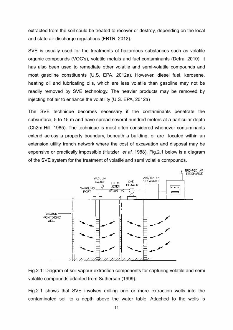
expensive or practically impossible (Hutzler et al. 1988). Fig.2.1 below is a diagram
of the SVE system for the treatment of volatile and semi volatile compounds.
Fig.2.1: Diagram of soil vapour extraction components for capturing volatile and semi
volatile compounds adapted from Suthersan (1999).
Fig.2.1 shows that SVE involves drilling one or more extraction wells into the
contaminated soil to a depth above the water table. Attached to the wells is

12
equipment such as a blower or vacuum pump, which pulls the air and vapour
through the soil up the well to the ground surface for treatment. The vacuum
monitoring well monitors the pressure of the air and vapour in the unsaturated zone.
SVE treatment can be applicable in both in situ and ex situ conditions. The latter is a
development of the in situ technique, the difference is that the soil would be
excavated for treatment and the treatment will be on the subsurface. Air is moved
through a stockpile of excavated contaminated material to promote volatilisation or
biodegradation of contaminants from the soil.
The SVE process requires a system for handling off gases. If the contamination
penetrates to the saturated zone or water table SVE and air sparging are often
considered at the same time to clean up both groundwater and soil (U.S. EPA,
2010a). Air sparging is an in situ physical/biological method involving the injection of
air (or other gases) below the water table to enhance volatilisation or biodegradation
of contaminants from the soil, water and the vapour phase (U.S. EPA, 2010a). There
are different types of soil vapour extraction systems which differ from each other by
the method used to transfer heat to the contaminated soil, and by the gas treatment
system used to treat the off-gases. The most popular method includes dual vapour
extraction, dual-phase extraction or multi-phase extraction (Defra, 2010). This SVE
method entails the use of a high vacuum system to remove contaminated soil or
groundwater.
The SVE process requires a system for handling off gases, this is necessary
because the volatile organic compounds typically present are hazardous due to their
toxicity and ignitability (U.S. EPA, 2006). In most cases direct discharge of the gases
without regulated treatment is unacceptable due to health, safety and public
concerns. The reason for pre-treatment of gases before discharging to the ambient
air is to improve the off-gas quality with minimal impact to human health or the
environment (U.S. EPA, 2006). The treatment technologies for off-gas treatment are
classified into four main groups by the (U.S. EPA, 2006):
Thermal – oxidation at high temperatures, contaminants are destroyed in
the vapour-phase.
Adsorption – the process of separating contaminants using a medium
13
or matrix Granular Activated Carbon (GAC).
Biological – use of living organisms to consume or metabolize
chemicals in the off-gas.
Emerging technologies – entail photocatalytic and non-thermal plasma
treatment, which destroy contaminants using ultraviolet (UV) light and
electrical energy respectively.
The selection of any off-gas technology depends on the nature of the distribution of
the contaminants in the subsurface, the site attributes and physical properties of the
chemical constituents and the overall remediation strategy. For example the thermal
oxidation system could be used to treat a wide range of SVE gases and is often
considered for VOC’s such as petroleum products due to its reliability in achieving
high destruction of the contaminants with good removal efficiency (U.S. EPA, 2006).
The system can oxidize from 95 per cent to more than 99 per cent of the influent
VOC (Bostrom, 2004). The three general type of thermal oxidation system include
direct-flame thermal oxidizers, flameless thermal oxidizers and catalytic oxidizers.
The potential advantages of SVE include its cost-effectiveness, the technique can
induce physical and biological processes, it is effective at removing many types of
pollution that can evaporate, it has minimal site disturbance and can treat many
organic compounds including diesel. In general, the wells and equipment are simple
to install and maintain and they can reach greater depths than methods that involve
digging up the soil (U.S. EPA, 2001). However, some hydrocarbons such as
petroleum products and contaminants with low water solubility are harder to volatilize
(U.S. EPA, 1996a). Other factors that may limit the applicability and effectiveness of
the SVE process include the presence of inorganic compounds and soil with a high
organic content (FRTR, 2012).
In addition, the applicability of SVE would most often depend on a field-pilot study
and high costs may be incurred to collect sufficient data that is required to design
and configure the system (U.S. EPA, 2012a). As well as costs associated with the
process, the excavation and material handling may pose hazardous emissions to the
surroundings, as exhaust air from the SVE system will require treatment to eliminate
possible harm to the public and the environment. Soil that has a high percentage of

14
fines and high degree of saturation will require higher vacuum or hinder the
operation of in situ SVE, which will also mean increased costs. In addition, due to off-
gas treatment, if residuals are condensed to a liquid or solid it may require treatment
or disposal, especially spent activated carbon which may need regeneration or
disposal. Despite these limitations the SVE technique has been technically
demonstrated and widely used and it has been selected for use in many superfund
sites in the United States of America (U.S. EPA, 2010a).
The technique has less environmental disturbance, is cost-effective and could be
used by facilitating extraction of higher concentrations of the contaminants when the
mass removal rate has reached an asymptotic level. Other remediation measures
such as natural attenuation or bioremediation can be adopted for further clean-up if
the remediation objectives have not been met. The technique could be used with
other methods depending on the circumstances and the remediation objective to be
achieved. For example the technique has proven to be effective in conjunction with
air sparging when groundwater is contaminated with evaporative compounds (U.S.
EPA, 2010a).
In the U.K., soil vapour extraction is normally considered when the contaminants
spread several hundred meters, extend across a property boundary, where there is a
high concentration of contaminants beneath a building or in an urban area where the
cost of re-location may be high. Soil vapour extraction can be applied to in situ and
ex situ conditions using physical and biological methods, although its usage in the
U.K has been limited (Defra, 2010).
2.5 Thermal desorption
Thermal processes use heat to increase the volatility, burn, decompose, destroy or
melt contaminants (NFESC, 1998). The technology is a thermally induced physical
separation process where contaminants are vaporised from a solid matrix and
transferred into a gas stream where they can easily be treated (Defra, 2010).
Thermal desorption is a new technology that permits on-site decontamination of the
soil by heating the contaminants to a temperature level where the chemicals
vaporise to a gaseous phase. This gas stream is collected or treated and even in
some cases heated to a higher temperature which destroys the contaminants.

15
Thermal desorption can be carried out on-site (without excavating the soil) as the soil
is heated to increase the removal efficiency of the contaminants, as illustrated in Fig.
2.2 and is referred to as in-situ thermal desorption (Baker et al. 2011). Ex-situ
thermal desorption is a similar process to the in-situ method with the exception that
the soil is excavated or stockpiled and introduced as a feed material. The ex-situ
system involves some pre- and post-processing of the soil especially when using
Low Temperature Thermal Desorption (LTTD) (U.S. EPA, 2012b). Excavated soils
are first screened to remove objects greater than 2 inches in diameter, which may be
crushed or shredded (U.S. EPA, 2012b). This means that the contaminated material
must be excavated from its original location following some degree of material
handling. Contaminated soils are excavated and transported to stationary facilities or
mobile units for treatment (U.S. EPA, 2012b).
Thermal desorption has been used widely in the U.S.A. for more than 12 years to
treat contaminated soil from gas plants (William and Brankley, 2006). In the U.K.
there are a number of sites where thermal desorption techniques are being
implemented and the regulators consider this as a viable alternative to landfill
(William and Brankley, 2006). Thermal desorption is also known to be highly effective
in treating soils contaminated with VOC’s, SVOC’s (semi-volatile organic
compounds), PAH’s, PCB’s, pesticides, cyanides and hydrocarbons and could be
applicable for in- situ and ex -situ conditions (Defra 2010).
The thermal desorption process applies heat to the contaminated media such as
soils, sediment, sludge or filter cake, to evaporate the contaminants into a gas
stream that is treated or managed. The treatment processes that are normally used
include: condensation, collection and combustion of the gases (U.S. EPA, 1996b).
The collection and condensation are usually treated off-site and combustion
treatments are carried out on the site following capture of the gasses. A typical site
has the following components as described in Figure.2.2 below:

16
Fig.2.2 Illustration of an in-situ thermal conducting heating system adapted from
Baker et al. (2011).
As shown in Figure 2.2 energy transfer is by thermal conduction and fluid convection
around the heaters as the heater bore is heated to an appropriate temperature. The
components comprise of a transformer that supplies power to the heaters, electrical
distribution controller for the heaters, vapour recovery wells, temperature and
pressure monitoring wells including an off-gas treatment system.
There are four main methods for in situ thermal treatment. These include injection
heating (hot air), electrical resistance heating, electromagnetic heating
(radiofrequency or microwave) and thermal conductive heating (FRTR, 2007; Unified
Facilities; CL: AIRE TD24 cited in Defra, 2010 and U.S EPA, 2006). The efficiency of
different thermal treatments will depend on applicability, the type of contaminants
and soil or groundwater conditions.
The fundamental principles of thermal desorption are to increase the temperature in
the ground which may promote contaminant removal by extraction or destruction.
Subsurface conditions can be conducive to easy degradation or managed for

17
disposal. Due to different operating temperatures thermal desorption can be
categorised into two groups. High temperature thermal desorption (HTTD) with
contaminants heated between 6000F to 12000F, and low temperature thermal
desorption (LTTD) with contaminants heated between 3000F to 6000F (NAVFAC,
1998). For in situ low temperature thermal desorption similar to Fig.2.2 the target
temperatures are in the range of 200OC to 350OC, depending on the physical and
chemical properties of the limiting contaminant (Johnson et al. 2009). The
applicability of the two different temperature conditions could be a function of soil
type, the depth of the contaminated matrix and the type and amount of contaminants
present (U.S.EPA, 2006).
The usual duration for VOC’s, such as diesel oil, is between 2 months to 1 year
depending on the site-specific requirements and the chosen heater spacing
(Johnson et al. 2009) and most projects usually take 1 to 2 month for demobilization
of equipment and restoration of the soil. But in a case where time is a determining
factor, the chosen technology and heater spacing can be varied to match the
expected project schedule at the expense of high energy usage. For instance in the
U.S. this is typically carried out for brownfield sites to be developed for the
construction of new homes Johnson et al. (2009) this is similar to the conceptual site
being evaluated in the study reported here.
The technology could be appropriate for complex sites in the U.K. such as
hydrocarbon contaminated sites where contaminants are not readily treatable and
the technique could be used especially in cases where quicker clean-up is needed or
where subsurface heterogeneities potentially limit the performance of other in situ
treatment alternatives. In addition, the technology allows soil to be cleaned on site
and reduces movement of vehicles transporting soils to landfill thereby saving fuel
and exhaust emissions which may be an environmental concern for most remedial
options in the U.K. However, the technology could be expensive as cost is driven by
energy and equipment costs and both are capital intensive (operation and
maintenance) and because the technique enhances the mobility of contaminants it
might lead to their migration outside the treatment zone.
2.6 Biological methods for hydrocarbon remediation
Current legislation, both in the EU. and U.K., in conjunction with economic drivers

18
has driven the search for alternative means of remediation for soils contaminated
with hydrocarbons. Bioremediation techniques have gained acceptance in the
remediation industry for the clean-up of chemically contaminated land (Jorgensen, et
al. 2000) and the technologies have been demonstrated to be feasible, quick, and
deployable in a wide range of physical settings. Soil bioremediation may be broadly
divided into in-situ and ex-situ techniques. According to (Xu and Lu, 2010) ex-situ
techniques include landfarming, composting, bioslurry and biopilling which are
carried out above ground using tilling, turning and applying oxygen and nutrients. In-
situ techniques involve the same biological treatment as ex situ but without
excavating the contaminated soil (Jorgensen et al. 2000).
The concept of the technique is based upon the enhancement of populations of
microorganisms either in the soil, or added to the soil to degrade the contaminants
(hydrocarbons). The technique gained popularity after the Exxon Valdez oil spill in
Alaska in 1989 (Margesin and Schinner, 1997). It was reported by Pritchard (1990)
that the Exxon Valdez spill was the cornerstone for a major study on bioremediation,
especially through the application of nutrients such as fertilizers.
The incident has confirmed that field studies provide the most convincing
demonstration of the effectiveness of bioremediation for oil polluted soils, whereas
laboratory studies do not account for the numerous real world situations
encountered. For example, the laboratory studies conducted by Bento et al. (2005) in
which all three technologies of bio-stimulation, bio-augmentation and natural
attenuation were evaluated and it was found that the number of diesel-degrading
microorganisms and heterotrophic population was not influenced by the
bioremediation treatments. Rather soil properties and the indigenous soil microbial
population affected the degree of biodegradation.
In a field study conducted by Venosa et al. (1992) on the Exxon Valdez oil spill it was
found that during a 27 day trial there was no significant difference between bio-
stimulation, bio-augmentation and natural attenuation. However, In a similar study of
the same Exxon Valdez spill the use of oleophilic (oil eating microbes) micro-
emulsions with urea as a nitrogen source, laureth phosphate as phosphate source,
and oleic acid as a carbon source and Customblen (reagent), used as nutrients for
shoreline treatment and applied over 120 km of the contaminated shoreline for

19
approximately 2-3 weeks, was investigated. The result from this second study
showed that remediation of the treated shoreline was greater than the natural
attenuation shoreline (Pritchard and Costa, 1991).
The practicality of bioremediation techniques was also shown during the Gulf war in
1991, when a huge amount of oil was spilt by the Iraqi soldiers returning from
Kuwait, covering about 770 km2 of the western coast of the Arabian Gulf and about
50 km2 of the Kuwait desert with crude oil from over 700 damaged oil wells (Cho et
al. 1997). After the incident there were arrays of field and laboratory studies to clean
up the soil and as such the efficiency of bioremediation techniques was fully tested.
Radwan et al. (1995) carried out a field study for a period of one year with eight
treatment types and their findings showed that a mixture of oil polluted soil and 3%
KN03 solution proved to be most effective in reducing the extractable alkanes to
about one-third of the original readings. However, repeated addition of nutrients such
as sewage sludge was inimical to alkanes biodegradation due to soil acidity.
In a similar study in the laboratory using Kuwait contaminated soil Cho et al. (1997)
applied Hyponex (soil with nutrient) and bark manure as a basic nutrient for
microorganisms and applied twelve other kinds of materials and surfactants (baked
diatomite, microporous glass, coconut charcoal and an oil-decomposing bacterial
mixture) to accelerate the biodegradation of hydrocarbons during 43 weeks
incubation. The results show that 15-33% of the contaminated oil was decomposed
and amongst the materials tested coconut charcoal was seen to enhance the
biodegradation of the hydrocarbon.
Since the incidents of Exxon Valdez and the Gulf war much has been achieved in the
field of bioremediation both in laboratory and field studies. The incidents have
prompted the development and refinement of the techniques at both a large and
small scale and have been the subject of debate and research efforts in recent
years. The demonstration of the significance of indigenous bacteria in degrading oil
has been fully identified (Radwan et al. 1995). The three types of bioremediation
including natural attenuation, bio-stimulation or bio-augmentation have been
optimally exploited (see; Bento et al. 2005; Nichols and Venosa 2008; Sarkar et al.
2005).
Both the Exxon Valdez and the Kuwait oil spill have provided background information

20
on the chemistry and biological nature of contaminants. As such the use of microbial
activities and chemical fingerprinting of contaminants have taken the centre stage in
current and future scientific thinking. Currently, chemical data and biological
techniques are adopted in assessing and describing the rate of hydrocarbon
degradation. The result of biological and chemical analysis of bioremediation
treatments can prove to be a useful prediction on how bioremediation should be
assessed and offer transparent lines of evidence to describe degradation rates
(Diplock et al. 2009).
Consequently, any bioremediation process must demonstrate the removal of the
contaminants and the rate of degradation must be higher than leaving the soil in its
original state (Bento et al. 2005). Hydrocarbon bioremediation can be promoted
either by stimulating the indigenous microorganisms, by the addition of nutrients and
oxygen or inoculation of an enriched microbial consortium into the soil (Liu et al.
2011; Kauppi et al. 2011). After several decades of studies of bioremediation there
are three main approaches to hydrocarbon bioremediation: natural attenuation, bio-
augmentation and bio-stimulation (Balba et al. 1998 and Bento et al. 2005).
2.6.1 Natural attenuation
Natural attenuation is the soils natural ability to degrade the contaminants without
external inputs. Natural attenuation is a clean-up technology that makes use of
naturally occurring microorganisms to mitigate contaminants that are present in the
soil. This is referred to as intrinsic bioremediation (Moreira et al. 2013). Natural
attenuation basically relies on the natural assimilative capacities of the soil to act
upon the contaminants (Simarro et al. 2013) and prevent their migration. However,
the technique is slow and uncontrolled because the method relies on indigenous
microorganisms to degrade the contaminants (Kauppi et al. 2011).
2.6.2 Bio-augmentation
Bio-augmentation is the addition of a microbial consortium made up of bacterial
species that have previously been isolated from a hydrocarbon contaminated soil
(Taccari et al. 2012). Thus the population of microorganisms added have already
been shown to be capable of removing a wide variety of hydrocarbons from the soil.
The ability of micro-organisms to degrade hydrocarbons has been known for many

21
years and Zobell, (1946) identified over 100 microbial species from 30 genera that
could degrade some type of hydrocarbons. These organisms are found in the
environment and are widely distributed in fresh and salt water, soil, and groundwater
(Borden et al. 1995). In practice the technique of bio-augmentation involves the
introduction of microorganisms that have been selected, for their ability to breakdown
hydrocarbons, and then cultured in the laboratory to increase numbers before being
added to the contaminated soil. These organisms may have been derived from the
existing contaminated soil or could have been obtained from a stock of microbes that
have been previously certified to degrade hydrocarbons. Once the microorganisms
enter the soil they selectively consume the hydrocarbons (Sarker et al. 2005) and
use them as a source of energy (Huang et al. 2013).
The bio-augmentation process may be enhanced by the addition of nutrients
essential for microbial growth, if soil analysis shows them to be lacking (Tsai et al.
2009). Nutrients commonly added are nitrogen and phosphorus (Gong, 2012).
However, the use of genetically engineered microorganisms, for use in
bioremediation, has seen little development over the past decade (Sayler and Ripp,
2000) due to ethical considerations and a lack of motivation from regulatory agencies
(Miller, 1997).
2.6.3 Bio-stimulation
Biostimulation is the introduction of nutrients in the form of organic and/or inorganic
materials into the soil. Natural attenuation is often limited due to the absence of
essential nutrients needed by the micro-organisms for growth; bio-stimulation is the
addition of these nutrients to optimise bacterial growth. The nutrients added could be
either organic or inorganic such as nitrogen and phosphorus (Sarka et al. 2005) or
other growth-limiting co-substrates (Nikolopoulo et al. 2013). Bio-stimuation
techniques have been shown to improve the biodegradation of oil under Antarctic
conditions and proved to be beneficial using nutrients and best experimental design,
constituting a promising alternative for some hydrocarbon-contaminated Antarctic
soil restoration (Dias et al. 2012).
The concept of bio-stimulation is that the addition of nutrients into the soil will
stimulate and increase the population of indigenous microorganisms. According to
Sarker et al. (2005) the indigenous microorganisms may or may not remove the

22
hydrocarbons from the soil or use it as a source of energy, but it is assumed that the
degradation occurs more quickly in comparison with natural attenuation as a result of
increased numbers of microorganisms due to increased levels of nutrients.
2.6.4 Factors affecting bioremediation
The environment exerts a significant influence on microbial activities and whilst
micro-organisms are present in any contaminated soil (Lee et al. 2012) the
availability of contaminants to the micro-organisms is influenced by a range of biotic
and abiotic factors. Factors that influence microbial degradation include: the
indigenous microbial populations; nutrient availability; oxygen; pH; temperature;
water content; bioavailability of contaminants and soil properties (Margesin and
Schinner, 1999; Taccari et al. 2012). During the bioremediation process the
optimisation of these factors will lead to the effective degradation of pollutants.
1. Temperature: This is an important abiotic factor for successful bioremediation of
contaminated land. Temperature exerts an influence on the nature and extent of
microbial hydrocarbon metabolism (Chang et al. 2010). In many temperate and cold
climates the degradation of aliphatic hydrocarbons is hindered by low ambient
temperatures during most of the year (Ferguson et al. 2008). Thus, some
environments are associated with extreme temperatures either in artic or semi-arid
regions. The U.K. is associated with cold temperatures during the winter and this
may limit the use of bioremediation.
In colder regions the rate of hydrocarbon degradation is seen to be very low and as
such the removal of hydrocarbons from the soil may be difficult and the contaminants
may remain in the ecosystem over a long period of time. In a study of bioremediation
of hydrocarbon contaminated soils in cold temperatures, such as the artic region
Whyte et al. (1998) noted that there was an increase in the viscosity of the oil in cold
climates and this reduced the movement of the oil through the soil thereby reducing
the chance of micro-organisms acting upon it.
However, there are cold-adapted indigenous hydrocarbon degraders in cold artic
regions because there are certain bacteria species that able to grow and metabolize
hydrocarbons over a wide temperature range (Chang et al. 2010). But a comparison
of oil decontamination at 100C to results reported at 250C – 300C underscores the
23
effectiveness of cold –adaptive degraders (Margesin, 2000). This shows a correlation
between decreasing temperatures and decreasing rates of enzymatic activities,
which are responsible for oil degradation. High temperatures tend to favour the use
of thermophilic bacteria for biodegradation of hydrocarbons. High volatilization and
solubility of some hydrocarbons at optimal temperatures influences toxicity and
allows biotransformation at high substrate concentrations (Whyte et al. 1998).
2. Oxygen: Most petroleum hydrocarbons are biodegradable under aerobic
conditions (Thapa et al. 2012). Oxygen can be seen as a co-substrate for enzymes
that catalyse the metabolism of hydrocarbons (Young, 1984). During bioremediation,
hydrocarbons are known to be oxidized (donate electrons) and an electron acceptor
(e.g oxygen) is reduced (Borden et al. 1994). There are a number of other known
electron acceptors including nitrate, iron oxide, water, sulphate and carbon dioxide.
In the bioremediation process if oxygen is depleted microorganisms may use other
oxidizing agents as an electron acceptor. However, oxygen is the preferred electron
acceptor due to microbial ability to obtain more energy from aerobic reactions.
3. Nutrient availability: The addition of nutrients to soil is to increase soil structure
and optimise the moisture content (Chang et al. 2010 and Abioye et al. 2012).
Nutrients commonly added are inorganic such as nitrogen and phosphorus (Chang
et al. 2010). But as the field of bioremediation continues to expand the application of
organic compounds becomes more popular in order to aid the metabolism of soil
microbes. In recent times bulking agents such as wood chips, vermiculite, animal
droppings, compostable municipal waste, poultry manure and other green wastes
are now used as nutrient supplements in the bioremediation of contaminated soil
(McMahon et al. 2008; Adesodun et al. 2007 and Defra, 2005 ).
4. Bioavailability of the contaminants and Indigenous microorganisms: One of
the challenging tasks of effective bioremediation is the ability of microorganisms to
degrade the contaminants to a residual point where it can be considered harmless to
the environment. The indigenous microorganisms are known to degrade
hydrocarbons more effectively than the introduced strains. This is because the
introduction of external oil degrading bacterial or known hydrocarbon degrading
bacteria may take a longer time to acclimatize to the contaminated environment.
In a laboratory experiment conducted by Cho et al. (1997) using contaminated soil

24
from the Kuwait desert, of the ten treatments they studied, the samples with oil
decomposing bacterial mixtures impeded the bioremediation process. In another
study by Radwan et al. (1995) using the same Kuwait desert contaminated soil, the
introduction of oil degrading bacteria was not effective in the removal of the
hydrocarbons from the soil whilst the optimization of indigenous oil degrading
bacteria demonstrated a significant reduction of hydrocarbons from the soil.
More so, in a study conducted by Kim et al. (2005), where three treatments
including the application of surfactant, oil-degrading bacteria and monitoring of
indigenous bacteria were evaluated it was found that the application of oil-degrading
bacteria in a concentration higher than the indigenous microbial populations
significantly increased the clean-up process. These finding’s to some extent
emphasize the role of dominance in microbial populations in terms of remediating
polluted soils. The indigenous organisms are known to have a niche within the
hydrocarbon contaminated site because they use the carbon as a source of energy.
As such if external bacteria are introduced they must be in a large quantity and have
the ability to dominate their indigenous counterparts. However, if the remediation
entails a large area the cost and complexity of using external bacteria could involve a
huge resource. There may also be regulatory concerns about the use of genetically
modified organisms.
5. Soil properties, pH, and water content: Environmental parameters such as
temperature, pH, moisture content, soil properties, quantity and bioavailability of
contaminants and redox potentials are significant for bioremediation (Fountoulakis et
al. 2009 and Margesin, 2000). The ability of the micro-organisms to adapt to the
environmental properties of the soil is a function of the nature and activity of the soil
bacterial community.
However, the modification of the environmental parameters could enhance bacterial
growth or survival. For example the measurement of pH in a soil is important to
understand the types of microbial species within that soil. This is because each
species of bacteria have their optimum pH value for growth. Thapa et al. (2012)
asserted that microbial growth and activity are readily affected by pH, temperature
and moisture. More so, soil pH may depend on other environmental factors such as
mineral and water content.

25
One important soil property in the bioremediation process is the value of moisture
content. Thus, water is an essential component in cell processes as it aids the
transportation of nutrients to the microbes. It also, serves as a medium for microbial
growth and regulates soil temperature. The water content in a soil can be determined
by measuring the soil water holding capacity.
Another dominant feature of soil properties is the clay-organic matter complexes.
The aggregation of the clay and organic matter complexes is an important element
governing microbial activities in soil matrices (Paul and Clark, 1998). The
composition of the clay-organic matter determines the availability of water infiltration,
oxygen tension and nutrient movement as required by microbial communities.
2.6.5 Disadvantages of bioremediation
In spite of the increased number of research studies investigating the use of
bioremediation, it has yet to be accepted as a routine treatment technology and the
environmental industry including the legislature are still wary of adopting the method
for the treatment of sites contaminated with hazardous chemicals. If bioremediation
offers benefits over other technologies, why has it not been more widely adopted to
treat environmental contamination?
One reason often put forward is that the physiochemical treatments are quick and
their outcome is predictable in the short term (Defra, 2010). More so, they are
relatively inexpensive considering the time frame required for bioremediation.
According to Juhassz et al. (2000) one of the difficulties of developing bioremediation
strategies lies in achieving as good or better results in the field as in the laboratory.
In addition there are numerous studies in the field of bioremediation that have shown
that out of the thousands of chemical compounds, in oil, only a few fractions are
known to be susceptible to biological degradation. Several bacteria and filamentous
fungi have been reported to detoxify and degrade hydrocarbons (Borras et al. 2010).
Fractions of hydrocarbon that have been shown to be biodegradable according to
Huang et al. (2013) includes; alkenes, aromatic hydrocarbons and polycyclic
aromatic compounds. These compounds are used by hydrocarbon degrading
microorganisms as carbon sources, breaking them down into fatty acids and then
into carbon dioxide (Prakash and Irfan, 2011; Haritash and Kaushik, 2009 and

26
Huang et al. 2013).
However, in a study conducted by Serrano et al. (2010), it was found that the
addition of a mixed bacterial consortium (Bioaugmentation) did not significantly affect
the biodegradation efficiency for polycyclic aromatic hydrocarbons (PAH’s) with low
molecular weights. Similarly a field study carried out by Garcia-Blanco et al. (2001)
on the shoreline of the St. Lawrence River found that the augmentation of nutrients
(biostimulation) did not have any major effects on the clean-up processes especially
when the oil had permeated significantly into the sediment.
In any bioremediation process the rationale for the application of exogenous
bacterial to the soil may be that the indigenous bacteria may not have the ability to
degrade the contaminants. But the importation of cultured bacteria strains is
assumed to lead to improved degradation, as the added culture are able to survive
and express their oil-degrading ability in the environment to which they are applied.
Bioremediation has been described as a multi-variable process, and the optimization
of the process through classical methods was inflexible, unreliable and time
consuming (Huang et al. 2013). One of the arguable shortcomings of bioremediation
is the unpredictability of the process, due to a lack of understanding of the behaviour
of microbial populations in natural environments and how physical, biological and
chemical factors interact to control their ability to breakdown environmental
pollutants.
One of the difficulties associated with bioremediation is the inability to effectively
evaluate the biodegradation process of the different bioremediation techniques due
to physical and chemical weathering, which may significantly affect the composition
and concentration of oil contamination (Nichols and Venosa, 2008). This could be as
a result of the polluted area being exposed to the contamination over a long time
period or at a newly polluted site the oil could be lost due to volatilization, adsorption
to organic compounds and other abiotic factors that are equally involved in the
reduction process (Adesodun and Mbagwu, 2008).
2.7 Monitoring and measurement of bioremediation
Evaluating the success of bioremediation may involve chemical, microbiological and
ecotoxicity assessment of soil polluted by oil, in order to improve the understanding

27
of the pollutants, microbial community dynamics and ecotoxicological effects of
various bioremediation strategies (Llado et al. 2012). Oil has been described as a
highly complex assemblage of organic compounds that no single analytical method
can entirely characterise (Al-Mutairi, et al. 2008). Hence the measurement of the
effectiveness of the bioremediation process may be inaccurate. It has been
suggested that the efficiency of the bioremediation process should be evaluated
using a chemical and toxicity test both during and post-remediation (Al-Mutairi et al.
2008). Llado et al. (2012) also state that acute toxicity tests would confirm the
improvement in the quality of the soil to give an insight into the progress of
bioremediation strategies.
Toxicity testing during bioremediation and post-bioremediation may serve as an
indicator of soil quality and the potential risk the contaminants pose to the natural
ecosystem (Margesin and Schinner, 1997). In a field study conducted by Salanitro et
al. (1997), evaluation of earthworms, seed germination and plant growth were used
to monitor total petroleum hydrocarbon (TPH) degradation. Their findings showed
that remediated soils were not toxic to earthworms and did not inhibit seed
germination after 10-12 months of treatment. The study showed that contaminated
soils could lose their toxicity and the potential to leach contaminants if successfully
bioremediated.
In recent times the measurement of hydrocarbon concentration by crop yield has
opened a frontier in the field of bioremediation, as plant growth has successfully
been used to measure the remediation of contaminated soils rather than as a
measure of soil toxicity. This emerging technology in many literatures has been
referred to as phytoremediation (Moreira et al. 2013). Phytoremediation is a low-cost
process based on microbial activation in the root zone and is regarded as a novel
method employed to remediate contaminated soil with VOC’s and SVOC’s (Defra,
2010).
At present there is no evidence of a universal TPH clean-up standard that can be
adopted, rather the efficiency of the clean-up is assessed using criteria based upon
risk-based assessments coupled to an evaluation of the environmental fate and
effects of the pollutants (Salanitro et al. 1997). In the United Kingdom the
contaminated land regime which is set out in part IIA of the Environmental Protection

28
Act 1990 (DETR, 2000) provides a risk based approach to the identification and
clean-up of sites which are considered to be contaminated. The risk to humans or
the wider environment is evaluated and land is only considered to be contaminated if
there is a source, pathway and receptor. The part IIA regime bestows the
responsibility for the identification and clean-up of contaminated land on local
authorities as the primary regulators (DETR, 2000). Appropriate remediation will
prevent, minimize or mitigate the effects upon human health and the environment. In
terms of hydrocarbons the commonly used measure under the U.K. regime is
chemical and biological assessment.
Most monitoring studies for bioremediation rely on the outcome of chemical analyses
such as gas chromatography or mass spectrometry to evaluate efficacy and infer
residual oil toxicity (Barthe, 1986). Therefore, there is a range of both chemical and
biological techniques that could be used to measure the efficiency of hydrocarbon
degradation both during and post-bioremediation. If the chemical and biological
assessment proved a degrading rate of contaminant concentration, then the
timeframe for the target to be achieved can be predicted.
The timeframe for a bioremediation objective to be achieved depends on the various
factors described (section 2.6.4.) above. In the review of Maila et al. (2005) the
success of bioremediation of TPH sites was noted in addition to their efficiency in
terms of percentage degradation of the TPH. Table 2.1 shows the duration of various
treatments of biostimuation and bioaugmentation which ranges from 3 months to 3
years depending on the treatment and contaminant types.

29
Bioremediation
techniques
Efficiency (%) of
oil removal
Microbial process including
the pollutant
Duration
References
11
Bio-augmentation
60 days
Lee et al. 2011
36.28%
Bio-stimulation
42 days
Ameh et al. 2012
83-93
Bio-stimulation PAH’s
161 days
Greenwood et al. 2009
78
Bio-stimulation PAH’s
90 days
Picado et al. 2001
75
Bio-stimulation
118 days
Benyahia et al. 2005
83
Bio-stimulation
126 days
Dadrasnia and
Agamuthu, 2012
92
Bio-stimulation
84 days
Abioye et al. 2012
Table 2.1: Reported success rates for bioremediation of TPH from different sites using bio-stimulation
and bio-augmentation including the percentage degradation and duration of the bioremediation process
Table 2.1 reports the results of studies into the bioremediation of hydrocarbon
contaminated land both in the U.K. and globally, which have indicated a period of 3
months to 3 years for the bioremediation objective to be met. Also in a study
conducted by PWTB (1999) in which samples from a variety of military operations in
Washrack were incubated and analysed, it was found that degradation levels
recorded met the reuse of soil level requirements in 6 months.
Another study in the U.K. where former gasworks sites owned by British Gas were
remediated (volume of treatable material 33,534 m3) the contaminants including
hydrocarbons were degraded and the site clean-up target was achieved in 6 months,
for all contaminants, at a trigger level recommended by the Environmental Agency
(Day et al. 1997). Another study that confirmed the efficacy of the bioremediation
process was the fieldwork conducted by Picado et al. (2001) in Portugal in which the
overall soil treatability of hydrocarbon contaminated soil detected a reduction of
30
PAH’s with 2,3,4 rings by 79 % within the period of 3 months.
The use of micro-organisms to remove hydrocarbon pollutants has been established
for decreasing the concentration of contaminants and reducing the risk to human
health and the environment. However, the use of the technique as a remedial
strategy at contaminated sites is still unpopular amongst remediation practitioners.
There are though strong drivers to increasingly adopt bioremediation as an effective
method to mitigate hydrocarbon contaminated soils (Diplock et al. 2009).
As such, chemical and biological data could be used to evaluate the efficiency of the
technique and could provide the regulatory body the metrics required to adopt the
technique as the most effective method to monitor oil contaminants from aquifers.
More so, assessment should provide a reasonable time frame for the remediation
objective to be achieved and should offer a transparent line of evidence to explain
degradation rates including the endpoint of the remediation target. Thus, laboratory
experiments must be effectively extrapolated to the field scale and biological
assessment and quantification of the bioavailability of hydrocarbons to bacteria,
degraders and heterotrophs should allow the evaluation of how bioremediation would
be measured (Diplock et al. 2009).
Therefore, the next section contains a review of some commonly used approaches,
some of which will be adopted to test the efficacy of the bioremediation technique
being evaluated in this study.
2.7.1 Biological techniques
Extensive efforts have been made in the field of bioremediation to investigate the
role of enzymatic reactions during the degradation of contaminated soil (Kaplan and
Kitts, 2004; Perry, 1984; Salminen, 2004; Venkatesan and Senthurpandian, 2006;
Zhang et al. 2006). Soil enzyme activities could then be used as indicators of
contaminant degradation as it incorporates information about microbial status and
the physicochemical condition of the soils (Chen, et al. 2003).
In the field of agriculture soil enzymes are often used as a biological marker of soil
fertility (Venkatesan and Senthurpandian, 2006) and the measurement of enzyme
activity in contaminated soils could also be used as a measure of changes in the
composition, structure and activity of microbial populations (Kaplan and Kitts, 2004).
31
The mechanisms underpinning the degradation of hydrocarbons, in the soil, are the
stimulation of growth and activity of hydrocarbon degrading micro-organisms in the
rhizosphere (Frick et al. 1999). Enzymes such as phosphatases, proteases, ureases
and pectinases secreted extracellularly by the micro-organisms into the soil could be
used as a measure of microbial activities (Venkatesan and Senthurpandian, 2006).
Measures such as microbial biomass and enzyme activity could be used to assess
both the health of the soil and the efficiency of the bioremediation process (Dick and
Tabatabai, 1992). Microbial plate counts on differing media will give an indication of
the populations of micro-organisms present whilst soil enzyme assays will give an
indication of microbial activities. Enzyme assays commonly used to assess the
efficacy of bioremediation include proteases, phosphatases, soil respiration and
dehydrogenases.
1. Protease Enzymes
Proteases are degradative enzymes that catalyze the hydrolysis of proteins (Ali and
Dahot, 2009). They are produced by a range of bacteria, actinomycetes and fungi
(Glenn, 1976). Protease activity is directly affected by the availability of carbon and
nitrogen (Geisseler and Howarth, 2008). The activity of protease has been described
in the literature. Kumar and Takagi (1999) asserted that soil proteins are hydrolysed
to peptides and amino acids by extracellular proteases. While Ali and Dahot, (2009)
described proteases as degrading enzymes that hydrolysed nitrogen compounds to
ammonium using urea and low molecular weight protein substrates.
Proteases have been extensively used in numerous fields but in bioremediation
protease activity could provide a better understanding of the biochemical processes
occurring in soil and demonstrate how biological parameters possess the potential to
act as sensitive indicators of soil ecological stress and restoration.
2. Phosphatase enzymes
The absorption of phosphate from organic compounds by micro-organisms and
plants is catalysed by the enzyme phosphatase. If concentrations of hydrocarbon
contaminants are high in the soil, phosphate is known to be a limiting nutrient for
microbial growth during bioremediation (URL1) hence concentrations of phosphatase
may be low. In the field of bioremediation it has been used to determine when

32
indigenous microbial populations are deficient in phosphate.
3. Dehydrogenase enzymes
Dehydrogenase enzymes are vital in the oxidation of organic matter in that they
transfer hydrogen from the organic substrate to the electron acceptor (Balba et al.
1998). More so, dehydrogenase may be used to measure process performance by
monitoring changes in the composition of the contaminants and biochemical process
parameters during bioremediation (Gong, 2012).
4. Soil respiration
In soil ecology, soil respiration is increasingly used for various purposes including the
diagnosis of the state of the soil in agricultural management. Respiration analysis
provides information on the biochemical processes occurring in the soil and is seen
as an important ecosystem process that releases carbon from the soil in the form of
carbon dioxide. Abiotic factors such as temperature, moisture and nutrient content,
as well as the level of oxygen uptake in the soil can all dictate the rate of soil
respiration.
In studies of bioremediation the possibility of obtaining basic information on the
biodegradability of contaminated soils, in terms of the supply of carbon, for microbial
growth and metabolism are well established (Nelson et al., 1996; Pagga et al. 1995).
Another study by Gomez and Sartaj (2013) measured the CO2 concentration inside
biopiles along with TPH percentage degradation. The results suggested that there
was biological activity inside the biopiles, confirming the successful adaptation of the
inoculated bacteria in the soil, which improved the efficiency of hydrocarbon
degradation.
Jorgensen et al. (2000) evaluated three different composting treatments using bark
chips, two commercial microbial inocula and nutrient amendments, in a field scale
trial, on a diesel oil contaminated soil. Three different treatments were evaluated by
measuring soil respiration rates. It was found that the treatment with the addition of
large amounts of organic matter produced more CO2 than the treatment with mixed
microbial inocula. Respiration as with enzyme activity can detect microbial activity in
the soil. It could therefore be used as a measure of the breakdown of hydrocarbon
contamination.

33
5. Microbial enumeration
In studies investigating the bioremediation of contaminated soil microbial counts are
normally carried out in order to determine both the numbers and types of
microorganisms present in the soil. They can be used to distinguish between fungi,
bacteria and actinomycetes (McMahon et al. 2008).
During bioremediation the identification of hydrocarbon degrading bacteria through
microbial counts can provide useful knowledge on soil biological activities and the
extent to which the indigenous microbial populations have acclimated to the site
conditions (Balba et al. 1998). The counts will also show if the soils have indigenous
microbial populations with the potential to support the bioremediation process. The
growth media most often used are mineral agar, malt agar, chelate mineral media
and R2A agar.
The field of bioremediation is expanding and over the past decade progress has
been made in terms of the identification of the various bacteria genera capable of
degrading hydrocarbon compounds at the field scale. Simarro et al. (2013) studied
the decontamination of creosote contaminated soil through microcosm assays,
evaluating changes in the bacteria community and toxicity. They characterised the
microbial population using deoxyribonucleic acid (DNA) extraction, molecular and
phylogenetic analysis.
The identification of species of bacteria with the aid of culture-independent molecular
biological techniques offers a new opportunity to better understand the dynamics of
microbial communities. Nucleic acid based molecular techniques for fingerprinting
the 16S ribosomal DNA of bacteria cells for the detection, description and
enumeration of bacterial targets has gained wide attention in modern microbial
ecology (Morales and Holben, 2009) and this approach is sometimes followed by the
sequencing of the gel bands to isolate the bacteria that are directly related to the
degradation of contaminants (Ciric et al. 2010).
2.7.2 Chemical analysis
The development and advancement in chemical fingerprinting and data interpretation
technique provides the opportunity for petroleum mixtures to be fractionated by
chromatography. The techniques have been used to monitor the distribution pattern
34
of petroleum hydrocarbons, analysis of source-specific marker compounds,
diagnostic ratios of specific oil constituents (Wang et al. 1999) and determination of
TPH levels in the soil (Moreira et al. 2013). There are a variety of techniques used to
screen soils contaminated with hydrocarbons including diesel, PAH’s and other
petroleum constituents, however, the use of chromatography has become popular.
This technique entails the separation of components in a mixture by partitioning
between a mobile phase and stationary phase. The types of chromatography
commonly used to screen or measure hydrocarbon constituents are:
2.7.3 Gas chromatography (GC)
This is a method for separating a mixture of compounds by partitioning the
components between a flowing gas (mobile phase) and non-volatile liquid phase
(stationary phase). GC is the most popular method and it is often used to screen
sediments for petroleum saturated and aromatic compounds and measure TPH. GC
can be used to determine the presence of petroleum compounds in a soil or water
and to qualitatively measure and examine their degradation rate (Wang et al., 1999).
GC has detectors such as the flame ionisation detector (FID), which is used to
measure TPH and an electro chemical detector (ECD), which is used to measure
chlorinated species. The GC-FID does provide a description picture of the major oil
components with the capability to monitor the effect of microbial degradation on the
loss of hydrocarbon at contaminated sites.
Another method is GC coupled with mass spectroscopy (GC-MS). The GC uses the
mass spectrometer to detect the components separated in the column. It can be
used to measure a sample in order to determine the pattern representing the
distribution of components (atom-molecules) by mass (mass to charge ratio). The
MS technique operates by bombarding a sample with electrons within a chamber
under vacuum. Then the molecules of the compounds become positively charged
due to the loss of electrons, forming fragmented ions, these fragmented ions pass
through a magnetic field where they are separated according to their mass. GC-MS
has a capillary that is capable of analysing the oil-specific biomarker compounds and
polycyclic aromatic hydrocarbons.
Other advanced methods for analysing hydrocarbon constituents are infrared
spectroscopy (IR), supercritical fluid chromatography (SFC), ultraviolet, isotope ratio

35
mass spectrometry and gravimetric (Wang et al. 1999 and Whittaker et al. 1996).
Adopting the improved analytical techniques to screen the components of petroleum
products to determine their concentrations depends on the total peak area between
a fixed retention times for the marker compounds, this gives the TPH concentration.
In the bioremediation process the concentration is usually calculated as a
percentage of degradation (Bento et al. 2005). Using chemical analysis to measure
hydrocarbons in soil would be as a result of degradation that is expected to occur
during the bioremediation process.
However, in an attempt to accelerate the degradation of the bioremediation process
nutrients could be added to augment the process and bio-waste could be added
(Abioye et al. 2012). Using waste in this manner will direct the flow of both
hazardous and biodegradable wastes from landfill to a sustainable reuse and offer
the opportunity for biodegradable waste not to be considered as residue, but as a
raw material for other processes. The next section will focus on waste management
in the U.K. and the use of biodegradable waste in bioremediation with the emphasis
being on BSG.
2.8 Waste management
The current combination of production, consumption and waste disposal in the world
is seen to be incongruent with sustainability principles. The current consumption
levels could be ascribed to a significant proportion of greenhouse gas emissions
emanating from the use of non-renewable resources, energy and water (WRAP,
2009). The goal of the United Kingdom government is to reduce waste, re-use,
recycle and recover value from wastes, which is an added value to the vision of the
living planet. These goals can be fulfilled if fewer natural resources are used and our
consumption of waste materials could be increased through re-use and recycling.
The U.K. government approach of the waste hierarchy is a strategy directed to all
parts of society from businesses, retailers, consumers, local authorities and the
waste management industry and requires them to take responsibility for the
management of waste (URL2) The waste strategy is meant to stimulate investment
in the infrastructure for the collection, recycling and recovery of waste and to improve
the market for recovered materials that would optimise value and energy recovered.

36
In the U.K. waste generation runs into 100 million tonnes ranging from household,
commerce and industry and most of the waste ends up in a landfill where the
biodegradable part generates methane a potent greenhouse gas (URL3).
In order to enforce the waste strategy the U..K Government has adopted the EU
Landfill Directive 99/31/EC which reduces the amount of harmful and biodegradable
waste going to landfill. The U.K. Landfill Regulation of 2002 is in compliance with the
EU Directive and states that by 2010, 2013, 2020 there should be a reduction in the
amount of waste sent to landfill of 75%, 50%, and 35% of 1995 levels respectively
(EC, 1999). The Directive targeted harmful and biodegradable waste which normally
results in emissions of greenhouse gases including methane and carbon dioxide.
The waste hierarchy bestows responsibility to various stakeholders in the waste
management industry including the following:
1. Prevention method: Whilst local authorities cannot stop consumers or retailers
from generating waste, businesses or manufacturers can build resource efficiency
into the business model to produce less waste by design. However, its total
prevention cannot be achievable.
2. Re-use of materials: This encourages the use of materials that would otherwise
become waste, which can provide a range of social, economic, and environmental
benefits (Defra, 2008). In the U.K. there are value driven organisations such as
voluntary and community organisations, charities, cooperatives, and social
enterprises that are involved in the process of re-use of waste. There are a 1000
third sector organisations working in the U.K. that participate in the re-use of un-used
material that would have been considered waste (URL3).
3. Recycle/recover: This is an initiative that encourages individual, corporations and
the waste management industry to reduce waste going to landfill. In the waste
strategy for England and Wales 2007, there are provisions for a voluntary code of
practice to set out guidelines for the provision of public access to recycling facilities.
The code of practice recommends five major elements that must be addressed for
recycling waste, they are:
provide recycling opportunities along with provisions for the correct disposal of
waste that cannot be recycled;

37
adopt standard signage on all recycle bins;
maintain and upkeep bins;
re-use, recycle and/
or compost the materials collected
Recycling now provides an avenue for the public to recycle their waste such as cans,
bottles and papers. The responsibility to maintain the recycling facilities rests with
the local authority, which in addition must provide a convenient recycling service for
household and commercial customers. In order to achieve this, the local authority
must invest in new infrastructure and provide local leadership and management for
waste. If a waste is not re-used or recycled then it could be composted as an
alternative to waste that cannot be physically recycled back to the system.
Composting of materials could take the form of anaerobic and aerobic breakdown
(Defra, 2007). Green waste composting is seen as a solution to the problem of
mitigating biodegradable waste volumes and to generate income from the sales of
compost materials (Probert et al. 2005 cited in McMahon et al. 2008). Compost
materials have become potentially useful in a wide range of applications such as
land reclamation, agriculture, top soil manufacturing, horticulture and home
gardening (McMahon et al. 2008).
4. Energy recovery: waste generation is unavoidable but the materials should be
seen as reusable resources. Waste such as feedstock, minerals, organic matter and
nutrients can be used for energy recovery (U.S. EPA, 1995a). The most common
source of energy recovery is through incineration and the capture of methane
generated at landfill sites. Incineration has become popular in most E.U. countries
due to it its energy recovery ability (Dijkraaf and Vollebergh, 2004). Incineration is the
controlled burning of waste at high temperatures. The organic constituents in the
waste are released as exhaust gas and the mineral matter is left as residual ash
(Dijkraaf and Vollebergh, 2004). In addition, landfill gas could be used to generate
electricity through the production of methane.
5. Disposal method: The EU landfill directive set thresholds that by 2010 the
amount of biodegradable waste going to landfill should be cut to 75% of the amount
produced in 1995; and by 2013 this should be reduced to 50% and by 2020 this

38
amount should be further reduced to 35% (Defra, 2005). Currently the final waste
disposal method is still dominated by landfill despite regional and national regulation
to curtail its popularity. It is often considered to be the worst option amongst the
waste hierarchy due to its use of space, high risk of leakages to air, water and soil
and that it releases less of the energy content of the waste as compared to
incineration (Dijkraaf and Vollebergh, 2004).
2.9 Classification of waste
In an attempt to manage waste, it is essential to identify and where possible quantify
the type of waste arising from various sources. Consequently, these classifications
will differ greatly in their economic potentials, their preferred disposal method such
as prevention, reduction, recycle and their final destination (Defra, 2011). In the U.K.
waste are classified by the Department of Environment Food and Rural Affairs
(Defra) The classifications include:
1. Agriculture waste: These wastes include pesticide containers, plastics such as
silage wrap, bags and sheet, packaging waste, tyres, batteries, clinical waste, oil and
old machinery. Agricultural waste includes a range of waste streams that originate
from agriculture or horticulture establishments.
2. Hazardous waste: This is a waste that contains hazardous properties that may
cause harm to human health or the environment. These include wastes resulting
from exploration, mining, quarrying, physical and chemical treatment of minerals.
Others are waste from agriculture such as horticulture, aquaculture, forestry, hunting,
fishing, and food preparation and processing. In addition, waste from wood
processing such as production of panel and furniture, pulp and paper, cardboard,
leather, fur and textile. Most Industrial waste comes from petroleum refineries,
natural gas purification, pyrolytic and treatment of coal. The list of hazardous wastes
is endless but can be accessed from the framework directives list put forward by the
European Union legislation.
3. Construction industry: This type of waste comes mostly from the demolition and
excavation sector. There is a major waste generation from the construction industry.
4. Inert waste: Waste is considered to be inert if it does not undergo any significant
physical, chemical or biological transformation. Inert waste does not dissolve burn or

39
otherwise chemically react. It does not biodegrade or adversely affect other matter it
comes in contact with. The total leachability, pollutant contact and eco-toxicity of inert
wastes are insignificant and do not pose any threat to the ecological system (WRAP,
2003).
5. Waste wood: These are wastes classified from sources in varying quantities and
levels of purity. There are 10 million tonnes of these types of waste produced in the
U.K. each year and the bulk of it goes to landfill (Defra, 2008). These types of waste
are regarded as biodegradable and they are generated mainly from the construction
and demolition sector, municipal solid waste and commercial and industrial sector.
BSG is a non-hazardous waste from the production of alcoholic and non-alcoholic
beverages (WRAP, 2010). The code for BSG in the European Waste Catalogue
(EWC) is 02 07 02 and it comes under waste from organic chemical processes
(WRAP, 2010). In the U.K. it is sold as an animal feedstuff, as a by-product, but in
excess it will go to landfill, hence in some circumstances it could considered as a
waste. In other parts of the world such as Asia it goes to landfill as a waste product
(Mussatto et al. 2006).
In the study reported here it will be used to evaluate the potential for the use of
biodegradable wastes in bioremediation because it was readily available. In addition,
BSG will also be used to evaluate the concept of using organic waste in the
bioremediation of contaminated land including their sustainability strands. These
evaluations are discussed in the next sections.
2.9.1 Brewery spent grain (BSG)
BSG is a type of industrial by-product from brewery processes all over the world in
both developed and developing countries. Other by-products of the brewery process
including spent hops, sludge, and yeast are all regarded as wastes (Levic et al.
2006). BSG is the most abundant brewery by-product, corresponding to about 85%
of the total 155 by-products produced (Tang et al. 2009). In the process of brewing
and packaging beer and spirits, such as whisky, the generation of by-products and
waste products is unavoidable (Levic et al. 2006). The annual world production of
beer is about 1.34 billion hectolitres and it is regarded as the fifth most consumed
beverage in the world after tea, carbonates, milk and coffee (Fillaudeau et al. 2006).

40
The EU are known to produce 3.4 million tonnes of BSG every year and the U.K.
produces over 0.5 million tonnes of this by-product annually (Stojceska et al. 2008).
BSG is of a high nutritive value and contains cellulose, hemicelluloses and lignin with
a high protein content, which varies according to its constituents. BSG is a
heterogeneous matrix comprising of a mixture of barley grain husk, pericarp and
fragments of endosperm (Forssell et al. 2008). It is the main by-product generated in
the brewing process, where barley malt is partially liquefied and the resultant liquor
(wort) is separated from the solid residues (BSG). The filtered wort is finally brewed
to beer. BSG has a high fibre content (cell wall carbohydrates) and is rich in proteins
and other minerals. This is due to the process of beer production when nearly all of
the starch is removed and the protein with other components become more
concentrated. The chemical composition of BSG is a function of barley variety,
harvest time, mashing condition, the quality and type of adjuncts used in the brewery
or the technology employed (Santos et al. 2003).
There are a number of reports on the constituents of BSG from different researchers
and biotechnologists. The protein and the lignin content in BSG depends on the raw
materials used and the processing method applied (Forssell et al. 2008). BSG
contains 31% of protein, 19% of pentosans, 16% of lignin, 12% starch and b-
glucans, 9% of cellulose, 9% of lipid, and 4% of ash (Prentice and Refsguard, 1978).
The chemical composition of BSG reported in several literatures was tabulated as
follows by Aliyu and Bala (2011):

41
Components
(% dry weight)
Kanauchi et
al.,(2005) Russ et
al.
(2005)
Mussatto and
Roberto (2006) Mussatto et
al, (2008) Adeniran et
al. (2008) Khidzir et al.
(2010)
Cellulose 25.4 23-25 16.8 16.8 - -
Hemicellulose - 30-35 28.4 28.4 - -
lignin 11.9 7.0-8 27.8 27.8 - -
Proteins 24 19-23 15.3 - 2.4 6.4
Ashes 2.4 4-4.5 4.6 4.6 709 2.3
Extractives - - 5.8 - - -
Others 21.8 - - 22.4 - -
Carbohydrates - - - - 3.3 -
Crude fibre - - - - 6.4 -
Moisture content - - - - - -
Lipid 10.6 - - - - 2.5
Acid detergent
fibre - - - - - 23.3
Total carbon (%) - - - - - 35.6
Total nitrogen (%) - - - - - 1.025
Table 2.2: Chemical composition of BSG as reported in the compilation of Aliyu and Bala (2011)
Due to the chemical composition and its varied attributes BSG has been found to be
useful in many fields including agriculture as animal feeds, in the food industry as
value-added compounds such as xylitric and lactic acid amongst others (Aliyu and
Bala, 2011) and because of its fibre rich and protein rich flour, it can be used as
ingredient in baking. Formulated foods are derived by grinding and sifting of dry BSG
(Chaudhary and weber 1990). It can also be used for microorganism cultivation or as
a raw material for extraction of compounds such as sugar, protein, acids and
antioxidants (Aliyu and Bala 2011). Apart from its usefulness in human nutrition and
animal feeds it could serve as alternative in biotechnological processes and for
energy production (Mussatto et al. 2006) and its use for the generation of biogas or
direct combustion are currently being investigated (Keller-Reinspach, 1992). In

42
addition, BSG possesses nutrients such as nitrogen, phosphorus and potassium (N,
P, K) which are limiting nutrients in hydrocarbon contaminated soil and these are
important elements for soil amendment and would be critical if used for
bioremediation.
2.9.2 BSG as a Bio-waste
BSG could be classified as an industrial waste according to the classification by
Defra. The Environment Agency, (2010) describe bio-waste as the biodegradable
components of municipal waste including organic industrial waste. Although BSG
could be put to many uses, it has received little attention as a marketable commodity
despite being produced in large quantities. Its disposal is often an environmental
problem (Mussatto et al. 2006). Brewery by-products including BSG are usually
disposed of to landfill where the organic carbon is converted into carbon dioxide and
methane (Mussatto et al. 2006).
There are numerous reports on the use of biodegradable waste to augment land
contamination in the field of bioremediation and it has been proved to be successful
for the bioremediation of contaminated soils (see Adesodun and Mbagwu et al. 2008;
Hickman and Reid, 2008; and Liebeg and Cutright, 1999; and Jorgenson et al.
2000). This technique becomes popular because the product provides nutrients for
microbial growth and hence enhances the breakdown of contaminants from the soil.
The current European Union directives that divert the amount of biodegradable
waste going to landfill coupled with the landfill tax have opened a new spectrum for
the alternative use of biodegradable waste. This study will discuss the options
available to utilise bio-waste for land remediation and consider how these fit into a
sustainable ethos with particular emphasis on BSG. The next section of this literature
review considers the sustainability of remediation of contaminated land and how
indicators for the measurement of sustainability could be developed.
2.10 Sustainability
Sustainability has been fully defined as ‘development, which meets the needs of the
present without jeopardising the ability of the future generation to meet their own
needs (WCED, 1987). The concept of sustainability could be seen to be product of a
national agenda because it encompasses all areas of national development. It

43
entails three strands – economic, environment and social (Defra, 2010).
Sustainability could be viewed differently by different groups of people depending on
the stakeholders involved. It is only through the understanding of the perspective of
each group that all stakeholders could come to a mutual agreement on a beneficial
intended goal. As such industrialised countries are becoming aware of the concept of
sustainability, with a broad-based government strategy being incorporated into the
economy from public to private projects. In most cases there is guidance on how
public sector proposals or projects should be appraised prior to commencement of
funding (Euro-Demo, 2006).
In the US for instance the strategy has been proposed in the ‘National Environmental
Act’ of 1969 compelling projects that have large impacts on the natural environment
and the rest of the society to be assessed (Moon, 2003). The US EPA developed
guidelines for preparing economic and environmental analysis of all costs and
benefits of private or public projects that affect the environment including social costs
(Moon, 2003). In the U.K. strategy for sustainable development, guidelines have
been proposed by HM treasury normally referred to as the ‘Green Book’. The book is
the best guide for all governmental departments and executive agencies and
includes projects of all types and sizes (HM Treasury, 2011). The goal is to promote
efficient resource allocation of any proposed government project and take into
cognizance of the wider social implications of the proposal.
The U.K. strategy for sustainable development has an aim of providing good quality
of life for present and future generations with objectives of maintaining a high and
stable level of economic growth without compromising the social progress and
effective protection of the environment. In other European countries, such as
Sweden and Norway the valuations of environmental projects have gained wider
attention and they are increasing in popularity in recent times (Moon, 2003).
In achieving the goal of sustainable development in the international scene there are
a number of initiatives that have evolved at a range of levels, international, regional
and nationally to protect human health and the environments. For example the
United Nation Framework Convention on Climate Change (UNFCCC) and Kyoto
protocol, have established a framework within which many countries, can take action
to mitigate the effects of Greenhouse gas (GHG) emissions. The countries that

44
signed up to the Kyoto agreement have committed to a domestic and national goal
by developing and promoting initiatives that will limit the volume of greenhouse
gases emitted given the targets set by the Kyoto agreement.
In addressing the three strands of sustainability there is a need for efficient
environmental regulations with empirical estimates of the costs and benefits of
environmental standards and policies (Cropper, 2000). The next sections will focus
on the application of sustainability to the remediation of contamination land and how
the three strands are measured.
2.10.1 Application of sustainability to remediation of contaminated land
Scientific information in the last decade suggests that global climate change can be
correlated with fossil fuel use and carbon dioxide releases into the atmosphere (Ellis
and Hadley, 2009) and remediation of contaminated land are usually associated with
the use of fossil fuel. As such, integrating sustainability into remediation projects has
attracted attention from remediation practitioners (Owsianiak, 2012). In the U.K.
there has been little work on the relative sustainability of remediation techniques
based on the evaluation of their wider environmental impacts (Harbottle et al. 2005).
The objectives of sustainable remediation is to achieve remedial goals using more
efficient, sustainable strategies that maximise resources and at the same time
protect air, water and land (Reddy and Adams, 2010).
However, the evaluation of all potential impacts in an integrated assessment process
are hardly achieved (Pollard, et al. 2001). This is because there is no single tool or
approach for identifying and evaluating the sustainability impacts of remediation
actions, as different tools focus on different elements of sustainability (Therivel,
2004). Thus, most remediation methods entail a wide range of activities that result in
environmental, social and economic impacts. In the past the most obvious impacts
are cost and duration and this informs the choice of appropriate technology
(Harbottle et al. 2005).
In the U.K. assessment of economic social and environmental impacts of
remediation is undertaken by an inter-government agency under the auspices of
Ministry of Environment. Policies and guidelines for assessing environmental
projects are directed by the Department of Environment Food and Rural Agency

45
(Defra), who provide a guidance role in setting the goals and objectives in achieving
sustainable remediation targets and it is the main repository of all U.K. remediation
data including sustainable indicators. The incorporation of all elements of
sustainability into decision making during site investigation, operation of treatment
systems, monitoring of treatment processes and progress and post remediation are
increasingly being promoted by the relevant governmental body. For example the
Environment Agency has produced guidance on the selection of remediation
methods, which allows the evaluation of the effects on soil, water, air and
ecosystems as a result of remediation processes (Postle et al. 1999).
There are varieties of tools used to evaluate the impacts or actions of remediation
methods and different tools are designed to deal with the different aspects of
sustainability (Therivel, 2004). However, there is no single tool or approach for
identifying and evaluating the sustainability impacts of any remediation method,
rather any tool should provide decision makers with information on how to minimize
any negative impacts or reject any actions with significant impacts (Thierivel, 2004).
Commonly used tools in the U.K. and elsewhere are cost and benefit analysis,
environmental impact assessment, cost-effective analysis, multi-criteria analysis,
sustainability analysis and life cycle analysis (EA, 1999, CL:AIRE, 2007, Hiester et
al. 2002; Moon, 2003, Owsianiak et al. 2012; SuRF-UK, 2010 and Therivel, 2004).
The adoption of any of these techniques should recognise all the embracing
concepts of the three strands of sustainability otherwise the agenda will fall short of
its ambitious objective.
The implementation of any remediation tool will necessitate the collection of data
covering the full range of sustainability issues. Data collection normally involves the
use of indicators relevant to the remediation activities. The next section will discuss
the metrics and indicators recommended to be used in the U.K. by Defra when
carrying out remediation projects.
2.10.2. Measurement of sustainable indicators in the U.K
The remediation techniques adopted in the U.K. show that the remediation industry
is still in its infancy in respect of measuring sustainability (Defra, 2010). CL:AIRE
(Contaminated Land: Application in Real Environment), developed a remediation
impact assessment tool on how to measure the sustainable elements of a project.

46
The tool is a spread sheet that stakeholders within the remediation industry can use
to assess sustainability of different remediation projects (SuRF-UK, 2010). The
parameters include pollutants, such as greenhouse gases, air, water, waste, and
environmental aspects of resources and people.
There is no single universally acceptable method of quantifying the impacts of
company activities on sustainability (Ellis and Hardley, 2009). But the Department of
Environmental Transport and Regions (DETR) in the U.K. provide indicators that
capture the link between economy and environmental performance. According to
Defra, (2008) there are 22 key performance indicators for U.K. businesses to
measure their environmental performance. These include:
a. Emissions to air
• Greenhouse gasses
• Acid rain, eutrophication and smog process
• Dust and particulates
• Ozone depleting substances
• Volatile organic compounds
• Metal emissions to air
b. Emissions to land
• Pesticides
• Metal emissions to land
• Acids and organic pollutants
• Waste (landfill, incinerator and recycling)
• Radioactive waste
c. Resource use
• Water use and abstraction
• Natural gas
• Oil
• Metals
• Coal
• Minerals
• Aggregate

47
• Forestry
• Agriculture
These are quantifiable metrics that reflect the environmental performance of the
economy. For stakeholders who want to measure their environmental performance
the appropriate use of these tools in alignment with recognised guidelines and
frameworks will demonstrate a progress toward sustainable development.
These set of guidelines are referred to as ‘Headline’ indicators of sustainable
development which increase the emphases on social implication of environmental
projects. The purpose of any environmental appraisal is not only to estimate the
costs and benefits but seek to refine possible options of achieving the same goal
with lower costs and greater environmental and social benefits. Since sustainability
is a relatively new concept in most segments of the developed world and even newer
to the remediation industry (Ellis and Harley, 2009), the Department of Environment,
Transport and Regions in conjunction with its inter-government agency, for many
years now, have provided guidance to the public and private sectors on how
environmental appraisal should be carried before funds are invested.
Recently, the U.K. sustainable remediation forum (SuRF-UK) provided a framework
document (SuRF-UK, 2010) on the mechanism for stakeholders to undergo
sustainability assessment using approved guidelines. These indicators do not
constitute a binding guidance for remediation practitioners but are recommended for
use when evaluating contaminated land and water. These indicators are described
below:

48
No. of impacts Environmental Social Economic
1
Impacts on air
(including climate
change
Impacts on human
health & safety;
Direct economic costs
& benefits
2
Impacts on soil;
Ethical &equity
consideration;
Indirect economic
costs and benefits;
3
Impact on water;
Impacts on
neighbourhoods or
region;
Employment and
capital gain;
4
Impact on ecology;
Community
involvement and
satisfaction;
Gearing
5
Use of natural
resources & generation
of waste;
Compliance with policy
objectives & strategies;
Life-span and project
risk
6
Intrusiveness.
Uncertainty and
evidence.
project flexibility
Table 2.3: Showing Categories of economic, environmental and social indicators
for sustainability assessment of remediation of contaminated sites adapted from
Defra 2010.
These 18 headline indicators for assessing soil and groundwater remediation were
developed by the United Kingdom’s Sustainable Remediation Forum (SuRF-UK) and
were obtained directly from the SuRF-UK report (2010). If these indicators are
optimally selected, designed and implemented remediation activities may impart
greater benefits than if the contaminants had been left untreated.
Generally, land and water remediation is embarked upon to mitigate risk to human
49
health including potential environmental, social and economic impacts. The process
of sustainable remediation necessitates an assessment of all aspects of remediation
processes. The process involves using indicators and other appropriate guidelines
and frameworks to measure the sustainability as recommended by Defra (2008).
The indicators are meant to address a range of issues that may be relevant and
provide assistance to practitioners to identify the most important factors associated
with the project that needs sustainability assessment. The indicators centre on the
three strands of sustainability which include:
1. The economic costs of remediation
Remediation costs have been viewed as site-specific due to the variability of
geological, hydrological, chemical factors and differences in remediation targets
(Defra, 2010). The economic costs of any remediation project are made up of the
direct costs of executing the project, which includes the costs of carrying out a
feasibility study, direct costs of labour, cost of acquiring land, cost of raw materials,
excavation or refill cost, landfill tax, and maintenance costs depending on the
remediation technology chosen (McEntee, 1991).
Other costs that cannot be easily quantified in remediation are the life span and
project risks. The economic cost of remediation is a major driver for the re-
development of sites in the U.K. in addition to the time frame for the remediation
objective to be met. If the remediation objectives are not on time there could be a
potential loss of investment and financial risk, especially if a loan has been obtained
to finance the project. However, the choice of meeting the objective is a function of
the remediation technique that is adopted. More so, costs that may be considered
include issues that could affect the work such as community disturbance,
contractual, environmental, procurement and technological risks, reputational
damage, energy use and waste generation (Defra, 2010).
Besides costs, there may be benefits that are associated with the remediation project
these include employment and capital gains of job creation. Others are skill levels
before and after remediation, and opportunities for education and training including
innovation and new skills. Some costs and benefits can easily be monetised
because they can directly be quantified by their activities and services. Whilst other
costs and benefits are difficult to assign a price to due to the difficulties of using

50
market metrics to quantify them, these include creating opportunities for inward
investment, use of funding schemes, and ability of the project to affect other projects
in the locality to enhance economic values.
2. Environmental costs
In appraising remediation projects the impacts encompass the life cycle of the
project and include: emissions, energy use, costs (direct and indirect), damage to
ecosystems, and emissions during and post remediation work. Measuring the
environmental impacts is an opportunity to assess the footprint of clean-up activities
throughout the life of the project.
Parameters included are: greenhouse gasses, air, water, waste and environmental
aspects of resources and people. In assessing environmental pollution in the U.K.
according to the Defra guidelines and framework, data are normally collected from
institutions such as the Department for Environmental Food and Rural Affairs (Defra,
2008), Department for Energy and Climate Change (DECC) and Devolved
Administration. The U.K. emission inventory is compiled by an inventory team AEA
technology (NAEI, 2008).
AEA compiled the data for the National Atmospheric Emission Inventory (NAEI) and
all types of atmospheric emissions from all sources (Mckinnon and Piecyk, 2009). As
the NAEI derives its data sources from the regulators, emission factors are typically
arrived at across range of sources that are representative of the sector. Emission
maps for the whole of the U.K. are routinely produced. These emission maps are
used by AEA and other organisations for a variety of government policy support work
at the national scale. Emission estimates in the U.K. are calculated by applying
emissions factors derived by NAEI to an appropriate activity.
3. The social costs of a remediation
This is a new phenomenon in the field of remediation which is still open to debate
both in terms of what the boundary is and the measurements that should be carried
out. In the SuRF-UK framework, social costs may account for social justice or
equality and questions that often surface are: is the spirit of the polluter pays
principle adhered to with regard to the distribution of impacts and benefits and are
the effects of works disproportionate to or more beneficial towards particular groups.

51
The social impacts may ask questions about the time scale of the impacts, if there
are issues of inter-generational equity and other ethical questions. Answers to these
questions determine the boundaries of how social costs should be measured.
The social element of sustainability may take the form of community satisfaction or
dissatisfaction, which cannot be measured generically, rather a qualitative
assessment is required to measure community satisfaction. In assessing social costs
the assessor must comply with policy objectives and strategies set by regulatory
bodies, codes of conduct set out nationally or by local authorities and/or in line with
industry working practices and expectations (Ellis and Hadley, 2009).
However, measuring the social elements of remediation is a difficult task to
undertake depending on the impacts that are being measured. There is a lack of
market to generate a price for such impacts, but the outcome for this lack of market
price is not accidental, rather markets are often missing this price due to the non-
excludable nature of the damage caused by the impacts. Although there are
economic techniques to establish monetary values for non-market impacts, they are
based on the inference of price. Money values for changes in biodiversity and direct
comparison with monetary values of alternative options, such as benefits of an
investment project certainly provide the bases for biodiversity policies (Nunes et al.
2001).
For example one way to assess the social benefits of removing toxic waste from a
site is to look at the impact of the site on adjacent house values over a given period
of time. House values generally are determined by the discounted value of the future
rents that would be accrued over time but if the existence of toxic waste at a site
causes rents to fall because the unit is less desirable then house prices close to the
site will decrease. Contaminated land or hazardous waste sites have a number of
local impacts, as residents will complain of odour, leachate, seepage, methane gas
build up, increased traffic flows, health risks, wind-blown litter, loss of visual
amenities and other environmental hazards. There is a high possibility that these
impacts could influence the value of local property. Social costs of remediation could
be captured and the impacts analysed in their respective nature and occurrences
(Kroeger and Manalo, 2006). According to Deaton and Hoehn (2004) there is a linear
relationship between property prices and distance from hazardous waste sites in the

52
U.S.A. However, if cleaning the site is carried out and all the environmental blights
are removed the price of houses located near the waste site is expected to rise.
Therefore, comparing the house value before and after the cleaning provides a
means of measuring the value captured as a result of the environmental
improvement.
2.10.3 Appraisal of the SuRF and Defra guidelines
In reviewing the recommendation of SuRF-UK, it is clear that some practices and
objectives of the guidelines can be achieved in any given remediation project.
However, it is not practical to implement all of the 18 indicators on every project in
that each remediation project is site-specific as the scenario in one site may differ
from other sites. As previously stated there are no standard metrics that currently
exist for assessing the relative sustainability of remediation alternatives.
In reviewing the environmental indicators recommended by SuRF-UK, many items
on the list can be converted into project metrics for sustainable remediation decision
making, provided all stakeholders agree on the approach at the inception of the
process when remedial alternatives are developed and considered. But there are
difficulties in agreeing on a particular approach in the remediation industry, at the
moment, because there are no regulatory standards and frameworks that
stakeholders must follow.
The lack of this framework can be seen in a review conducted under the guidance of
Defra (2010), in which a group of practitioners in the remediation industry were
surveyed, it was found that most of them evaluated their sustainability differently
using various techniques and matrices and they did not adhere to a particular
approach. Their decisions to assess their remediation impacts using different tools
and matrices was as a result of non-binding regulatory guidance that drives
remediation practitioners to use a particular approach on a project, even when the
project has the same inherent environmental, social and economic impacts.
At present the role of the regulator in the decision making process is limited and
advisory and practitioners evaluating sustainability of remediation projects are likely
to arrive at ambiguous or conflicting results for the same project given the same site
conditions (Ellis and Hadley, 2009). For example, there is no universally accepted
53
way of calculating the environmental element such as carbon dioxide and other
environmental footprints. This leads to the use of an array of carbon calculators
creating confusion and inaccurate information (Reddy and Adam, 2010).
In addition, the framework for measuring the environmental and social impacts
recommended by Defra/Surf still ignore some impacts especially when socio-
economic evaluation of the clean-up costs are due to secondary emissions or
community disturbance during remediation activities or the effect of existing
contaminants in that locality. However, the social matrices recommended by SuRF-
U.K. can comprehensively be adopted by remediation practitioners in the U.K. as
social impacts are usually measured by societal preferences, due to the absence of
market price. Most tools adopted for valuing social impacts are either revealed or
stated in the individual behaviour. Revealed or stated methods are based on impacts
on environment and human welfare (Randall, 1998).
The revealed and stated methods are popular in the U.S. and have been used to
examine the value of attributes that contribute to overall housing value, these
attributes include distance to hazardous waste site, environmental quality, such as
air pollution, odour and other negative externalities (Kiel and Zabel, 2001 and
Ihlandfeldt and Taylor, 2004). The valuation methods hinge on the economic value an
individual assigns to a particular goods or services (environment and social impacts).
This is commonly measured by the maximum amount of resources the individual
would be willing to give up in order to obtain the goods or services in questions
(Barbie, 2000). Most techniques chosen to value environmental goods are meant to
retrieve consumer’s preferences because the price of market goods generally
exhibits a clear value an individual places on them (Kroeger and Manalo, 2006).
In the U.K. social impacts occurring during the remediation process are not often
measured. Although scientific study does provide evidence of incremental noise
levels at certain municipal soil waste management facilities (composting, landfill and
gasification/pyrolysis) as well as noise and odour from landfill sites (Defra, 2005).
There are few or no studies that attempt to value social impacts during the
remediation process. This is because impacts such as community disturbance or
satisfaction, impacts on neighbours or the region and impacts on human health and
safety are difficult to quantify. It is not surprising that they are not measured given the

54
nature of the impacts. For example, there is no clear cut procedure of measuring the
remediation of a site that has a causal effect on the flow of traffic on adjacent roads
and this is often not taken into consideration when measuring social impacts on a
site.
Whilst coverage resulting from economic and environment impacts of the
remediation process is reasonable and comprehensive there are still large
uncertainties in the range of values provided for social impacts. It is difficult to use a
particular valuation method but some studies previously mentioned have used either
revealed or stated methods, in the US, allowing monetary values of social impacts to
be expressed. This will make it possible to compare, in common units the relative
health and environmental effect of different remediation methods.
Therefore, there is need to define the economic, social and environmental
assessments with appropriate guidelines and procedures to be followed, as this will
make sustainable remediation indicators more uniform even when measured by
different assessors.
2.10.4 Sensitivity analysis
This analysis focuses on how a conclusion on sustainability indicators depends on
certain assumptions that are used to arrive at the conclusions. In other words the
analysis tests whether the indicators used hold a wider confidence margin than
accounts for differences in measuring the impacts using various techniques. It has
been suggested that sensitivity analysis should be considered as an element of
sustainability assessment in order to determine the variation in input data and how
assumption can influence the overall outcome of an assessment (SuRF-UK, 2010).
These analyses are the inherent subjective values of the assessors, as it is possible
that different assessors presented with the same scenario and information may
arrive at a different assessment of the optimum solution. The purpose of the analysis
is to underpin the need for assessors to understand the variability of their data input
as any significant changes in certain inputs may alter the outcome of the
assessment.

55
2.10.5 Setting the boundaries of a sustainability assessment
Prior to undertaking a remediation sustainability assessment, there should be a
definition and agreed boundaries for the assessment (Ellis and Hadley, 2009). If
these boundaries are not pre-determined there is the possibility that different
assessors can make different assumptions in respect to the limit of the assessment
and this will make decisions difficult to achieve (SuRF-UK, 2010). The boundaries
should state which environmental, social and economic factors are to be taken into
consideration, and which benefits or impacts of the three strands should be
assessed. In addition the time/duration of the benefits/impacts of remediation of
contaminated land should be stated for example if it is 10years, 2 generations or
over 100 years and then the benefits/impacts should be measured over the agreed
timeframe. This all need to be considered at the initial stage.
2.11 Conclusions
Land contamination could be as a result of anthropogenic activities with most
pollution arising from past and present industrial activities. This has led to a number
of brownfield sites. Society has become attuned to the necessity of re-using
brownfield land for urban development.
There are a wide range of techniques that can be used to clean-up contaminated
brownfield sites including physicochemical, traditional and process based techniques
such as bioremediation and thermal desorption. The techniques used are associated
with activities that result in environmental, social and economic impacts; however,
there is growing recognition of the importance of making clean-up of contaminated
land more sustainable and thereby minimizing its economic, environmental and
social impacts.
Considering the sustainability of remediation projects has attracted attention from
remediation practitioners and other stakeholders and the three elements of
sustainability are increasingly being taken into account when a remediation
technology is being considered for use. Achieving sustainability in land remediation
is a current thinking in the circle of national sustainable development in the U.K. and
there is an expanding portfolio of initiatives, regulation, standards and guidelines
proposed by the U.K. Government through Defra. The purpose of sustainable
56
development in the remediation industry is to underpin the application of sustainable
principles through the development process of land regeneration and mitigate the
harmful effect of land contaminants posed to the environment and human well-being.
However, many brownfield development projects do not consider the ‘time’ costs of
redevelopment in terms of the sustainability of the potential remediation options. This
project will attempt to evaluate both the economic and environmental costs of
remediation using bioremediation with and without BSG as an example. The next
chapter reports on initial laboratory based investigation to determine the practicability
of this approach for diesel contaminated soils.

57
Chapter 3
MATERIALS and METHODS
3.1 Introduction
The aim of this chapter is to describe the methods used in the study and report on
the experiments carried out to evaluate them.
This entails a series of laboratory techniques including, those developed in the
laboratory for the analysis of the practical aspects of the remediation processes such
as soil preparation, experimental design and maintenance, microbiological methods,
analytical methods, statistical analysis and the evaluation of methods and
development of techniques.
Soil preparation describes how the soil was prepared before use including the
materials used in the study. The experimental design and maintenance describes
how the treatments were maintained throughout the experiment including
temperature, water added, pH recording and the amount of soil collected for
laboratory testing.
The microbiological methods describe the type of agar used in the study to
characterise the bacteria. R2A and oil agar were used in the classification of the
bacteria. The aim of choosing the oil agar was to investigate if the bacteria found in
the soil have the potential to degrade diesel. A similar study has been carried out by
Prakash and Irfan (2011) where bacteria that used crude oil as the sole carbon
source were characterised and their potentials to utilize the compounds in a mixture
of hydrocarbons as a substrate were determined. The R2A agar was used to
determine the bacteria counts in the treated soil. It is normally used to monitor viable
bacteria growth in environmental media (Pyle, et al. 1995).
The section on analytical methods describes how the sample from the treated soil
was chemically analysed using gas chromatography (GC) and describes the soil
extraction process prior to chemical analysis. It also describes the type of GC and
the analytical conditions used in analysing the soil.
The statistical analysis describes the types of statistical test used in the study and
the reasons for the choice of the different statistical tests.
58
The evaluation of methods and development of techniques includes the procedure
used for spiking the soil in the laboratory. This becomes necessary as the volume of
diesel that is to be added to the soil is small and as a result there is a need to
increase the volume of liquid, added to the soil, by diluting the diesel with another
solvent. This will ensure an even distribution of the diesel throughout the soil.
Acetone had been previously used in the laboratory to spike contaminated soil with
hydrocarbons (Sawada et al. 2004).
As such four solvents were investigated, including water, to determine which solvent
can homogenously mix the diesel in the soil. This development also involved the
determination of the percentage recovery of the diesel from the spiked soil. This was
carried out by adding a known amount of diesel to the soil and determining how
much can be recovered. A similar technique has been used by Cam and Gagni
(2001) to investigate the determination of petroleum hydrocarbons in spiked
agricultural soil using commercial diesel.
In addition, different percentage recoveries were compared. This was carried out to
determine if the amount of diesel recovered from the soil is proportional to the
volume added. In order to make these comparisons, different percentages of diesel
were added to a fixed amount of soil and the diesel compounds were extracted to
determine the amount recovered. This experiment is to further validate the
techniques of the study including the extraction procedures used for recovering the
diesel from the soil and the GC performance.
3.1.1 Laboratory work
A series of laboratory scale experiments were carried out to determine the
procedures to investigate if the addition of BSG would improve upon the degradation
of diesel contaminated soil with and without the addition of BSG, which was
investigated in chapter 4. The procedures include:
3.2 Soil preparation and experimental design
The soil sample used in all of the experiments was a loamy soil that was a mixture of
45% clay, 25% sand and 30% silt. This is an agricultural soil without any recent
nitrogen amendments. The soil was obtained from small organic farmland in Bowes
in Teesdale near Barnard Castle, U.K. The soil was initially sieved through a 2 mm

59
sieve to remove any stones or large particles. After the soil had been sieved it was
contaminated with diesel to the appropriate concentration. Full details of the method
used for the addition of the diesel can be found in section 3.7.1.
The contaminated soil was transferred into trays 30 cm in length and 21 cm wide.
The trays were covered with Goretex fibre, to replicate field scale remediation and
incubated at room temperature. The soil was not sterilised in order that the
indigenous microbial populations could be maintained. Three replicates of each
treatment were prepared. Before use the soil was subjected to chemical analysis
using gas chromatography (GC) to determine if the soil was free from hydrocarbon
contamination.
BSG was collected from Darwin Brewery, which is a micro-brewery with a capacity of
350 litres located at Enterprise Park in Sunderland. Prior to use the BSG was
collected and stored for 3-4 days at 40C, in the laboratory at the University of
Sunderland.10 litres of commercial diesel was purchased from a filling station in
Sunderland and stored at room temperature in a closed container. The same batch
of diesel was used throughout the experiments.
3.3 Experimental design and maintenance
Maintaining the experiments entailed routine mixing of the soil in the trays and
spraying it with water in order to maintain the soil moisture content. A constant
volume of water was added to the soil weekly throughout the experiment based on
the weight of soil in each treatment types. Water was sprayed onto the replicate
treatments to ensure that the soil did not become dry. The soil was aerated by
turning and mixing it thoroughly in order to achieve homogeneity of any amendments
added.
Three replicate samples were removed at a range of sampling times. From each
treatment 23.0 g of soil was removed for both microbial analysis and for the
determination of TPH.
The pH value of the soil was determined using a paste prepared by shaking 1 part of
the soil with 2.5 parts of distilled water (Hendershot and Lalande, 1993), readings
were taken using a Fisherbrand Hydrus 300 pH meter. Before the readings were
taken, the pH meter was calibrated using standard solutions.

60
3.4 Microbiological methods
3.4.1 Culture media
Microbial counts were performed using R2A agar and minimal (oil) media (Gong,
2012). The formulation of the R2A and oil media is represented in section 3.4.2. At
each sampling time 10 g of soil was mixed with 100 cms3 of 0.2% by volume
sterilised sodium pyrophosphate, for 30 minutes, at 200C using a shaker at 150 rpm
(Revolution per Minute). Thereafter 1 cm3 of the soil/pyrophosphate solution was
transferred into 9 cms3 of sterile saline solution and a ten-fold serial dilution was
carried out; that is from 10-1 to 10-10 according to the technique adopted in (Moreira
et al. 2013).
After the serial dilutions, 0.1 cms3 of the diluted solution was removed from each
sterile saline-soil/pyrophosphate mixture test tube and distributed onto petri-plates
containing R2A and oil agar media.
In the oil agar plate, a disc of filter paper impregnated with diesel was placed in the
lid of each plate. The diesel was used as a sole source of carbon for the organisms
to utilize (Balba et al. 1998). Both media plates were incubated at 250C and were
inspected after 24 hours for colony formation and thereafter every 24 hours. After 72
hours the number of colony forming units (CFU) per gram was determined (Gong,
2012). The colonies were counted using a bacterial count enumerating machine and
the results were recorded.

61
3.4.2 Formulation of media preparations used in the study
a) R2A agar
FORMULAE
Difco TM minimal agar Davis
Formula * per Litre
Grams
Yeast Extract 0.5
Proteose Peptone No. 3 0.5
Casamino Acids 0.5
Dextrose 0.5
Soluble Starch 0.5
Sodium Pyruvate 0.3
Dipotassium Phosphate 0.3
Magnesium Sulphate 0.05
Agar 15.0
Table 3.1: Composition and Formulation of R2A agar and concentration levels
measured in grams used in this study (URL 4).
R2A agar was developed by Reasoner and Geldreich (URL4) for bacteriological
plate counts of treated potable water and soil related heterotrophic micro-organisms
(URL4). The agar helps to stimulate the growth of bacteria of differing tolerances at a
lower incubation temperature and longer incubation times as it is nutritionally rich. It
has also been reported to improve the recovery of such micro-organisms (URL4).

62
b). Oil agar:
FORMULAE
Difco TM minimal agar Davis
Formula * per Litre
Grams
Monopotassium Phosphate 2.0
Dextrose 1.0
Ammonium Sulphate 0.5
Sodium Citrate 0.5
Dipotassium Phosphate 7.0
Magnesium Sulphate 0.1
Agar 15.0
Table 3.2: Composition and Formulation of oil agar and concentration level measured in
gram used in this study (URL5).
Oil agar is most suitable for growing selected heterotrophic microorganisms (Wrenn
and Venosa, 1996). In this media the carbon source is reduced unlike R2A agar and
other carbon sources such as hydrocarbons (including diesel) are added externally.
The micro-organisms which grow on this media would be able to breakdown the
diesel for their growth because of the minimal carbon present in the media itself
(Abioye et al. 2012). The agar was developed by Lederberg (URL5).

63
3.5 Analytical methods
3.5.1 Diesel extraction for gas chromatography
For each replicate sample 10 g of soil was collected according to Llado et al. (2012)
and weighed into a bottle and mixed with 20 cms3 of hexane. It was then placed in a
shaker at 100 rpm for 24 hours at room temperature. After 24 hours the samples
were filtered by vacuum funnel. Aliquots of the hexane extract were pipetted from the
bottle and sealed in a gas chromatography (GC) vial. Extracts were analysed as
soon as possible after extraction. If it became necessary to store the samples they
were kept at 40C. The method for the analysis of the hexane extract is described in
section of 3.5.2 below.
3.5.2 Chemical analysis of hydrocarbons
Hexane extracts were transferred to a vial of 1.5 cms3 for GC analysis using a (GC)
HP 5890, Hewlett Packard with a fused silica capillary column, equipped with a flame
ionization detector (FID), Agilent, USA (US EPA, 1995b). The column used was DB-1
(30m by 0.25mm) with nitrogen as the carrier gas, at a flow rate of 2 cms3 min-1.
The GC used in the study is shown in Figure 3.1

64
Fig. 3.1: showing Gas Chromatography (GC) HP 5890, Hewlett Packard with a fused
silica capillary column, equipped with a flame ionization detector (FID) which was
used in analysing the soil samples for all treatments in the study.
The temperature programme used was 650C min-1 60C min-1and 3000C for 2 mins.
This method was used throughout the experiments except experiment three (3) in
which helium was used as the carrier gas but all other conditions were maintained.
The extractable petroleum hydrocarbons were identified and quantified by
comparison of sample height and retention time to the control samples (blank
samples). Duplicates of control samples were run concurrently with the original
samples at 1:5. For every 5 treatment samples run a control sample was
concurrently run and any discrepancy between the control and the expected results
were analysed accordingly. Gas chromatography (GC) has been used by Paiga et al.
(2012) to determine the level of TPH in contaminated soils and the results of their
study demonstrated that GC had the capacity to accurately quantify TPH in soils,
irrespective of the contamination levels.
65
3.6. Statistical analysis used in the study
Test of significance for all results in the study
Statistical analysis used in the study was to determine the significant differences and
relationships between observed values. When a significance figure of (P<0.05) was
obtained the null hypothesis of no difference was rejected and the alternate
hypothesis of existence of differences in sample values was accepted.
Levenes’ test of homogeneity of variance was used to help determine the type of
statistical tests needed for the analysis and the results were further compared with a
Shapiro-Wilk test to test the normality of the data set. Histogram plots and Q Q plots
were also prepared. Although most of the tests were found not to be significant (p =
>0.05), some were significant (p = <0.05), which suggested a violation of the
assumption of normality (Pallant, 2007).
In the analyses paired t-test, independent t-test and the Mann–Whitney U test, which
is a non-parametric test were carried out. One way ANOVA a parametric equivalent
of Mann-Whitney U test was used where appropriate. However, despite the
Shapiro –Wilk test signifying that the data was non-normal, and some of the numeric
normality tests on the data appearing to give significant differences, a parametric test
as well as a non-parametric test were applied. This is because the distortions of
normality did not affect the tests ability to detect any differences and it has therefore
been possible to compare results from parametric and non-parametric tests and be
able to gain extra confidence from any conclusions drawn.
3.7. Evaluation of methods and development of techniques
3.7.1 Introduction
The purpose of these experiments was to standardize the methods to be used in the
main evaluation. First a procedure was developed to test the homogeneity of the
diesel in spiked soil using the same soil that would be used in future experiments.
This was carried out to ensure that the diesel was evenly distributed in the soil. The
second experiment was carried out to determine how much of the diesel added could
be recovered and the third experiment was to determine if the % recovered from the
soil is proportional to the volume of diesel added.

66
3.7.2 Soil spiking
As the volume of diesel that is to be added to the soil is small there is a need to
increase the volume of liquid, added to the soil, by diluting the diesel with another
solvent. This will ensure an even distribution of the diesel throughout the soil. The
soil was left in a fume cupboard for 6 hours to allow the volatile compounds to
evaporate. This first experiment was evaluated after the addition of the diesel/
solvent mixture and the most suitable solvent to be used in the study was
determined..
Table 3.3 represents the concentration of diesel and solvents including water used to
dilute the diesel.
Solvent Name Soil (g) Vol. of diesel
added to the
soil (cms3)
Vol. of solvent
(cms3)
Number of
Trays
Acetone 2000 200 80 3
Methanol 2000 200 80 3
Hexane 2000 200 80 3
Water 2000 200 80 3
Table 3.3: Showing grams of soil, diesel and solvents evaluated as possible
diluents for diesel.
The experiment comprises of four treatments which were replicated three times. For
each sample 2 kg of soil was placed in a tray. The solvents or water were added to
the soil in the ratio 1:25 and the soil solvent mixture was added to the diesel. The soil
diesel mixture was then mixed thoroughly. The soil was then transferred into trays
and the mixture was left for 24 hours. Figure. 3.2 below shows the soil and the trays
used in the laboratory.

67
Fig. 3.2 showing replicate trays containing 2kg of soil which the diesel/solvent
mixture were added.
After the addition of diesel and solvents each sample was extracted for chemical
analysis as described in section 3.5.1 and 3.5.2.
Fig 3.3: Showing total peak height as a measurement of TPH C9 – C23 recovered
using the different solvents; acetone, methanol, hexane and water.
There was a statistically significant difference between treatments as determined by
one-way ANOVA F (3, 48) = 5.160, p = .004. The post hoc (LSD) test revealed that
recovery rates from soil contaminated with diesel mixed with acetone (M = 18.7 SD =
8.3 SE = 2.30), p = .001, diesel mixed with methanol (M = 18.6 SD = 8.0 SE = 2.2 ),
p = .001 and diesel mixed with hexane (M = 16.4 SD = 6.9 SE 1.9 ), p =0.013 were
0
50
100
150
200
250
Tto
tal p
eak
he
igh
t C
9 -
C2
3 c
ms
Peak height Acetone, 187
Peak height, Methanol, 186
Peak height, Water, 92
Peak height, Hexane, 164
Diluents
Peak height Acetone, 187cms
Peak height, Methanol, 186 cms
Peak height, Water, 92 cms
Peak height, Hexane, 164 cms
Diluents
Tray containing soil Soil diesel/solvent mixture
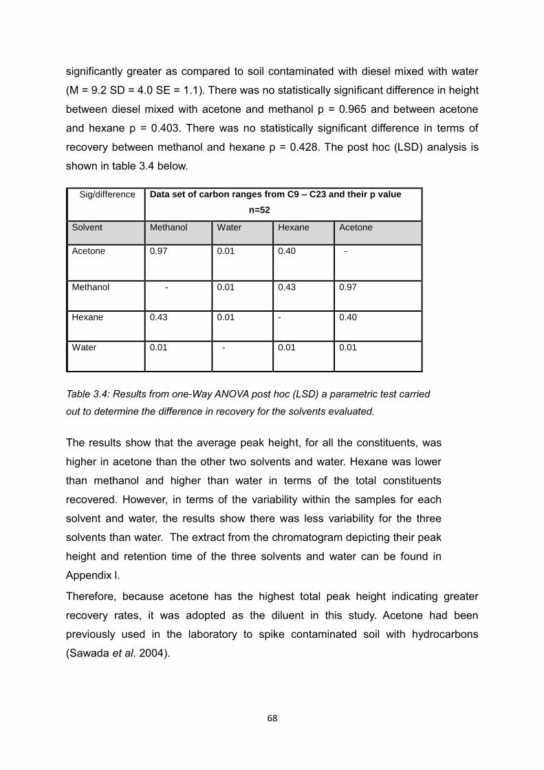
68
significantly greater as compared to soil contaminated with diesel mixed with water
(M = 9.2 SD = 4.0 SE = 1.1). There was no statistically significant difference in height
between diesel mixed with acetone and methanol p = 0.965 and between acetone
and hexane p = 0.403. There was no statistically significant difference in terms of
recovery between methanol and hexane p = 0.428. The post hoc (LSD) analysis is
shown in table 3.4 below.
Sig/difference Data set of carbon ranges from C9 – C23 and their p value
n=52
Solvent Methanol Water Hexane Acetone
Acetone 0.97 0.01 0.40 -
Methanol - 0.01 0.43 0.97
Hexane 0.43 0.01 - 0.40
Water 0.01 - 0.01 0.01
Table 3.4: Results from one-Way ANOVA post hoc (LSD) a parametric test carried
out to determine the difference in recovery for the solvents evaluated.
The results show that the average peak height, for all the constituents, was
higher in acetone than the other two solvents and water. Hexane was lower
than methanol and higher than water in terms of the total constituents
recovered. However, in terms of the variability within the samples for each
solvent and water, the results show there was less variability for the three
solvents than water. The extract from the chromatogram depicting their peak
height and retention time of the three solvents and water can be found in
Appendix l.
Therefore, because acetone has the highest total peak height indicating greater
recovery rates, it was adopted as the diluent in this study. Acetone had been
previously used in the laboratory to spike contaminated soil with hydrocarbons
(Sawada et al. 2004).

69
3.7.3 Percentage recovery
Recovery studies usually involve the addition of a known amount of analyte to a
sample and then determining what % of the amount can be detected (Sawada et al.
2004). In the study here the recovery rate was tested by adding a known amount of
diesel to a fixed amount of soil to determine the recovery %. In preparing the
experiment 1% of diesel was added to 1 kg of soil as described in the protocol in
section 3.5.1 and 3.5.2 and extracted in hexane solution. For comparison 1% of
diesel was extracted (not added to soil) in hexane solution as described in section
3.5.1 and 3.5.2. Both samples were replicated. The % recovery was determined by
comparing the percentage difference between TPH extracted from the soil diesel
mixture and that measured when the diesel was added directly to haxane.
Fig: 3.4: Recovery % of diesel when added to 1 kg soil under investigation, peak height is
based on carbons C9 – C23.
Figure 3.4 shows the average peak height of the treatment with 1% diesel without
soil and treatment with 1% diesel added to soil. The treatment with diesel only has a
total peak height of 41 cm, treatment with diesel and soil has a 28 cm level of peak
0
5
10
15
20
25
30
35
40
45
Tota
l pe
ak h
eig
ht
C9
-C2
3 c
ms
Diesel concentration, Diesel, 41 cms
Diesel concentration, Diesel + soil, 28 cms
1% diesel concentration

70
height. This is equivalent to 68% of the original diesel recovered from the soil. The
statistical test to show the significant difference is shown below.
An independent sample t-test indicated that the total peak height of diesel that was
added directly to the hexane was significantly higher (M = 219 SD = 128) than the
total peak height of diesel extracted from the soil (M = 80 SD = 43), t(20), 4.22, p =
.001, d = 1.18. Despite the differences between the samples the results showed that
the recovery % of diesel from the soil was 68% based upon a comparison of the
peak heights in figure 3.2. The remaining 32% could be attributed to volatilization
and evaporation of the diesel due to its volatile components.
3.7.4 Representation of the effect of concentration on % recovery
This is an analytical procedure to test the relationship between multiples samples.
This can be carried out by measuring known properties of different compounds in a
sample and the results are directly compared to the concentration (amount) of the
analyte in the sample (Harmonised, 2005). The aim here is to compare the
relationship between the different % recoveries to determine if the amount of diesel
added to the soil is proportional to the diesel recovered.
This experiment is to determine if the % recovery, as measured by peak height, is
proportional to the volume of diesel added. Diesel was added to 1 kg of soil at a
concentration of 0.5%, 1.5%, 2.5%, 3.5% and 4.5% (v/w) according to the spiking
procedures described in the protocol in section 3.7.1.Each of the diesel
concentrations was in triplicate as shown Figure 3.5 below:
Fig.3.5: showing replicate trays containing 1 kg of soil which the diesel/solvent
mixture were added at 1%, 1.5%, 2.5%, 3.5% and 4.5% concentration level.
After 24 hours the diesel was recovered by extracting in hexane as described in
Soil diesel/solvent mixture Tray containing soil
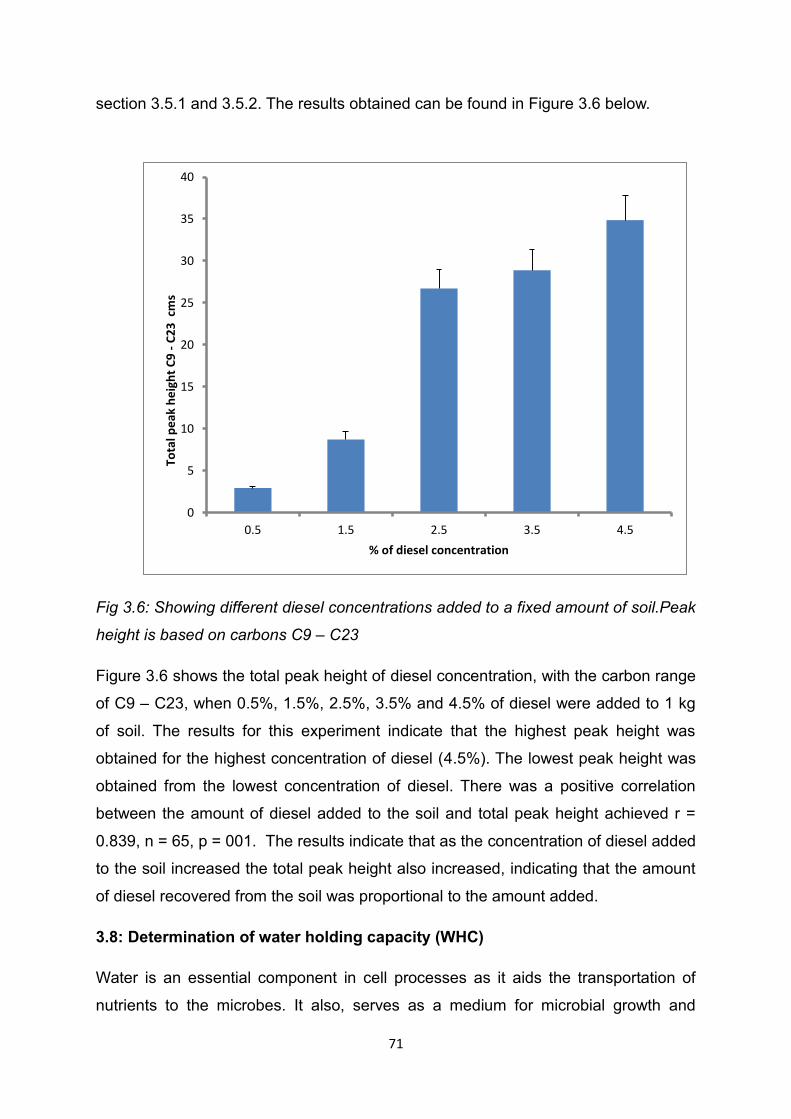
71
section 3.5.1 and 3.5.2. The results obtained can be found in Figure 3.6 below.
Fig 3.6: Showing different diesel concentrations added to a fixed amount of soil.Peak
height is based on carbons C9 – C23
Figure 3.6 shows the total peak height of diesel concentration, with the carbon range
of C9 – C23, when 0.5%, 1.5%, 2.5%, 3.5% and 4.5% of diesel were added to 1 kg
of soil. The results for this experiment indicate that the highest peak height was
obtained for the highest concentration of diesel (4.5%). The lowest peak height was
obtained from the lowest concentration of diesel. There was a positive correlation
between the amount of diesel added to the soil and total peak height achieved r =
0.839, n = 65, p = 001. The results indicate that as the concentration of diesel added
to the soil increased the total peak height also increased, indicating that the amount
of diesel recovered from the soil was proportional to the amount added.
3.8: Determination of water holding capacity (WHC)
Water is an essential component in cell processes as it aids the transportation of
nutrients to the microbes. It also, serves as a medium for microbial growth and
0
5
10
15
20
25
30
35
40
0.5 1.5 2.5 3.5 4.5
Tota
l pe
ak h
eig
ht
C9
- C
23
cm
s
% of diesel concentration
72
regulates soil temperature. The composition of a clay-soil and its organic matter
complexes govern microbial activities in the soil matrix (Paul & Clark, 1998). This
also, determines the availability of water infiltration, oxygen tension and nutrient
movement as required by microbial communities.
Calculating the water holding capacity (WHC) would enable the determination of the
volume of water that is needed to be added to the soil to enhance microbial growth
and maintain the soil structure. However, in the experiment here a consistent volume
of water was added to the soil to maintain the experiment and in all cases this was
85 cms3 for treatment without BSG and 176 cms3 for treatment with BSG in 1000 g
of soil, which is less than the field water holding capacity. The amount of water
added to the soil showed that the soil was moist but not waterlogged. The water
holding capacity for soil and BSG are calculated in Appendix 11 according to the
description in Grace et al. (2006) which is the water holding capacity expected to be
used in the field.
3.9 Conclusions
This chapter evaluates a range of techniques including those developed in the
laboratory for the analysis of the practical aspects of the bioremediation processes.
The methods covered were soil preparation and experimental design, experimental
maintenance, microbiological methods, analytical methods to be adopted, statistical
analysis and development of techniques.
The chapter also covered the use of various solvents to determine which solvent will
be used to increase the volume of diesel when spiking the soil in order to achieve an
even distribution of diesel in the soil. Acetone was adopted as the diluent to be used
throughout the experiment. The results from the chapter also showed that 68% of
diesel can be recovered from the soil when 1% of diesel was added to 1 kg of soil.
The method further showed that the amount of diesel added to the soil was
proportional to the amount recovered validating the extraction procedures and the
GC performance to be used in the main experiment (Chapter 4).
Therefore, the next chapter will evaluate if the use of BSG would improve upon the
bioremediation of soil contaminated with diesel fuel using the same methods.

73
Chapter 4
LABORATORY SCALE EVALUATION OF BIOREMEDIATION PLUS BSG
4.1. Introduction
The aim of this chapter is to investigate the use of BSG to improve the
bioremediation of soil spiked with diesel in the laboratory. Two experiments were
carried out - experiment (a) and (b). Experiment (a) investigated bioremediation,
including the addition of BSG to augment the bioremediation processes. The
experiment further studied the effects of the addition of a bacterial consortium.
Experiment (b) was a repeated bioremediation process to determine the consistency
of using the BSG, no bacterial consortium was added. The next sections will cover
the procedures used in carrying out the experiment, which includes a review of the
bioremediation techniques, methods, monitoring and maintaining the experiments,
microbial analysis, results of the experiment, discussions and conclusions.
4.1.1 Review of bioremediation techniques
The prerequisite for effective bioremediation of contaminated soil is the presence of
microorganisms able to degrade the contaminants (Suni and Romantschuk, 2004).
Several laboratory and field tests have demonstrated the effectiveness of
bioremediation in the clean-up of soil contaminated with hydrocarbons either using
indigenous microorganisms or by the inoculation of exogenous microbial consortia
(selected bacteria) (Benyahia et al. 2005, Lee et al. 2011 and Ameh et al. 2012).
A number of studies have focussed on the addition of organic wastes to improve
upon the bioremediation processes, these include the laboratory scale study
conducted by Cho et al. (1997) in which various nutrients such as Hyponex (compost
for soil amendment) and bark manure, baked diatomite, microporous glass and
coconut charcoal were used as a basic nutrient for microorganisms using Kuwait oil
contaminated soil. The purpose of the study was to accelerate the biodegradation of
hydrocarbons during 43 weeks incubation. The result shows that 15-33% of the
contaminated oil was decomposed and amongst the materials tested coconut
charcoal was seen to enhance the biodegradation of the hydrocarbons most
effectively.
74
A similar laboratory scale study was conducted at the Institute of Biological Sciences,
University of Malaya, Malaysia by Dadrasnia and Agamuthu (2010) to investigate the
biodegradation of diesel fuel in soil contaminated with 10% (w/w) diesel fuel
amended with 10% tea leaf, soy cake and potato skin for a period of 90 days (3
months). It was found in the study that 76% biodegradation of the oil was recorded
at day 84 with the treatment amended with soya cake. Whilst only 27% of the oil
was degraded in the control treatment. Potato skin and tea leaf recorded 64% and
53% biodegradation respectively.
The chapter reported here will focus on laboratory studies and seek to answer the
first objective of the study, does the addition of BSG improve upon the bacterial
breakdown of hydrocarbons and is the technique feasible? Therefore two
bioremediation experiments were carried out which include experiment (a) and (b),
the methods adopted are described in the next section. Experiment (a) was to
investigate bioremediation, including the addition of BSG to augment the
bioremediation processes, and the experiment was further studied with the addition
of a bacterial consortium. Whilst experiment (b) was a repeated bioremediation
experiment to determine the consistency of using the BSG no bacterial consortium
was added. Experiment (b) was carried out to further optimise the process by
studying the addition of BSG using different concentrations of diesel. The description
of the materials and experimental design employed in this chapter can be found in
section 3.2 to 3.8 in Chapter 3
4.2 Methods
Experiment (a)
The aim of this experiment was to investigate the remediation of diesel contaminated
soil using bioaugmentation and biostimulation in the laboratory. The composition of
the experiment consists of five treatment types as indicated in Table 4.1 below.

75
Treatment
Reference
% of diesel
in the soil
Grams of soil
+ diesel
Consortium
added
(cms3)
BSG grams
added (10%)
Number of
replicate
trays
1 -
1000
- -
3
2
0.5%
1000
- -
3
3
0.5%
1000
-
100
3
4
0.5%
1000
200
100
3
5
0.5%
1000
200
-
3
Table 4.1: Composition of the different treatments incubated in the laboratory including soil
only treatment, soil plus diesel (5,000 mg kg-1 soil), soil plus diesel (5,000 mg kg-1soil) plus
consortium, soil plus diesel (5,000 mg kg-1soil) plus consortium plus BSG and soil plus diesel
(5,000 mg kg-1soil) plus BSG
From Table 4.1 treatment (1) contains 1 kg of soil only and has no diesel or any
BSG. In treatment (2) 1 kg of soil was spiked with 0.5% diesel (v/w). The
composition of treatment (3) was made up of 1 kg of soil spiked by 0.5% diesel (v/w)
with the addition of 100 g of BSG. In treatment (4) 0.5% diesel (v/w) and 100 g of
BSG was added together with a microbial consortia at the rate of 20 cms3 of the
mature culture to 1000 g of soil. Treatment (5) contains soil with 0.5% diesel (v/w) in
addition to 100 g of BSG and 20 cms3 of the mature culture to 1000 g of soil. The
consortia in treatment 4 and 5 was sprayed onto the soil and then mixed evenly. The
bacteria used in the study are Achromobacter clevlandii and Stearothermophillus
rhizophila. The strains were supplied by Pattanathu Rahman from Teesside
University and had previously been characterised as hydrocarbon degrading
microorganisms isolated from contaminated river sediment. The layout of the soil
used is shown below in Fig. 4.1.

76
Fig. 4.1 showing replicate trays containing 1 kg of soil to which the diesel/solvent
mixture was added in the laboratory.
Diesel and BSG were added to the soil treatments as described above according to
the method detailed in section 3.2 and 3.7.1 Once prepared the trays were covered
with Goretex fibre to prevent evaporation of the diesel and incubated at room
temperature 180C to 250C for the period of the experiment. All of the experiments
were set up in triplicate.
4.2.1 Monitoring and maintaining the experiment
Maintaining and monitoring the experiment involved routine mixing of the soil and the
addition of water as described in section 3.3. Replicate samples were removed from
each treatment for microbiological enumeration and for TPH analysis. The same
protocol was applied for all treatments.
4.2.2 Microbial analysis
Quantifying the activity and number of aerobic microorganisms is an important step
in evaluating the bioremediation processes. In the study reported here microbial
counts were performed using R2A agar and oil agar as described in section 3.4.1.
4.3 Results of Experiment (a):
The findings from this study are presented in the following order.
4.3.1 TPH analysis
4.3.2 Statistical analysis
Soil diesel/solvent mixture
Tray containing soil
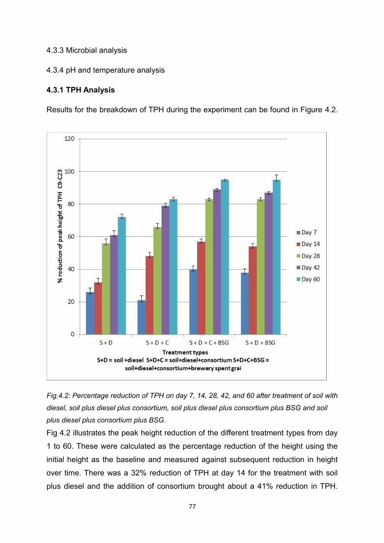
77
4.3.3 Microbial analysis
4.3.4 pH and temperature analysis
4.3.1 TPH Analysis
Results for the breakdown of TPH during the experiment can be found in Figure 4.2.
Fig.4.2: Percentage reduction of TPH on day 7, 14, 28, 42, and 60 after treatment of soil with
diesel, soil plus diesel plus consortium, soil plus diesel plus consortium plus BSG and soil
plus diesel plus consortium plus BSG.
Fig 4.2 illustrates the peak height reduction of the different treatment types from day
1 to 60. These were calculated as the percentage reduction of the height using the
initial height as the baseline and measured against subsequent reduction in height
over time. There was a 32% reduction of TPH at day 14 for the treatment with soil
plus diesel and the addition of consortium brought about a 41% reduction in TPH.
78
The introduction of BSG to the consortium resulted in a 56% reduction and the
treatment with soil plus diesel plus BSG also recorded a 56% reduction. At day 28
the treatment with soil plus diesel shown a reduction of 55% and the treatment with
soil plus diesel plus consortium has a reduction of 66% but the addition of BSG
brought about an 82% reduction in the total peak height. Whilst the treatment with
soil plus diesel plus BSG recorded an 83% reduction at day 28.
At day 42 the treatment with soil plus diesel has a reduction of 61% whilst the
addition of consortium led to a further reduction of 77% and the addition of BSG
resulted in an 89% reduction. The treatment with soil plus diesel plus BSG has a
TPH reduction of 87% at day 42.
Finally, at day 60 the treatment of soil plus diesel has a total reduction of 72% and
treatment with consortium has an 83% reduction. The addition of BSG to the
consortium led to a further reduction of 95% and treatment with soil plus diesel plus
BSG also recorded a total reduction of 95% at day 60 respectively.
4.3.2 Statistical results of TPH
The results from Fig. 4.2 above indicated that there were differences in the TPH
reduction in the various treatment types. Analysis of variance using one-way ANOVA
and a post hoc test to show the differences between the treatment types for day 1,
14, 28, 42, and 60 are presented below.
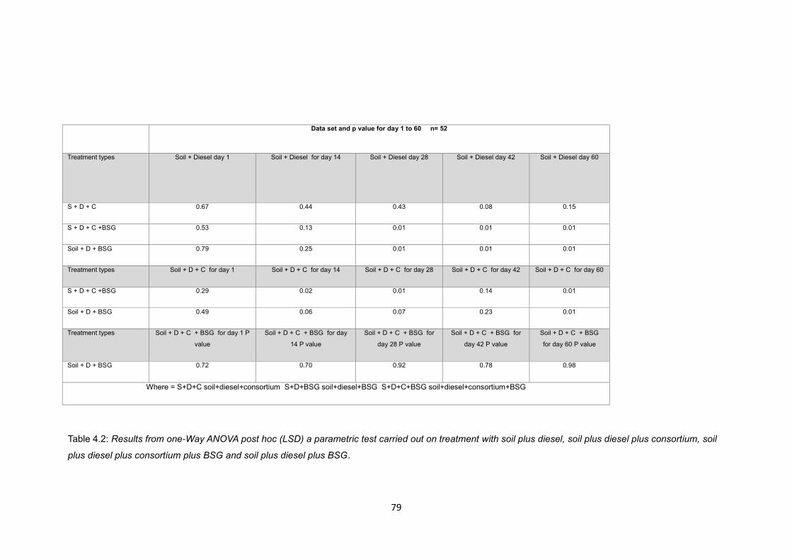
79
Data set and p value for day 1 to 60 n= 52
Treatment types Soil + Diesel day 1
Soil + Diesel for day 14 Soil + Diesel day 28
Soil + Diesel day 42
Soil + Diesel day 60
S + D + C 0.67 0.44 0.43 0.08 0.15
S + D + C +BSG 0.53 0.13 0.01 0.01 0.01
Soil + D + BSG 0.79 0.25 0.01 0.01 0.01
Treatment types Soil + D + C for day 1 Soil + D + C for day 14 Soil + D + C for day 28 Soil + D + C for day 42 Soil + D + C for day 60
S + D + C +BSG 0.29 0.02 0.01 0.14 0.01
Soil + D + BSG 0.49 0.06 0.07 0.23 0.01
Treatment types Soil + D + C + BSG for day 1 P
value Soil + D + C + BSG for day
14 P value Soil + D + C + BSG for
day 28 P value Soil + D + C + BSG for
day 42 P value Soil + D + C + BSG
for day 60 P value
Soil + D + BSG 0.72 0.70 0.92 0.78 0.98
Where = S+D+C soil+diesel+consortium S+D+BSG soil+diesel+BSG S+D+C+BSG soil+diesel+consortium+BSG
Table 4.2: Results from one-Way ANOVA post hoc (LSD) a parametric test carried out on treatment with soil plus diesel, soil plus diesel plus consortium, soil
plus diesel plus consortium plus BSG and soil plus diesel plus BSG.

80
Day1
There was no statistically significant difference between groups for the mean of
various treatment types as determined by one-way ANOVA F (3, 52) = 0.395, p =
0.757. The post hoc (LSD) test revealed that there was no significant difference
between the total peak height for treatment with soil plus diesel and soil plus diesel
plus consortium p = 0.670 and treatment with soil plus diesel plus consortium plus
BSG p = 0.534 and treatment with soil plus diesel plus BSG p = 0.790.
The treatment with soil plus diesel plus consortium did not statistically differ from
treatment with soil plus diesel plus consortium plus BSG p = 0.296 and treatment
with soil plus diesel plus BSG p = 0.490. There was no significant difference between
the treatment with soil plus diesel plus consortium plus BSG and treatment with soil
plus diesel plus BSG p = 0.721.
Day 14
There was no statistically significant difference between group means for the various
treatment types as determined by one-way ANOVA F (3, 52) = 2.190, p = 0.096. Post
hoc (LSD) test revealed that there was no statistically significant difference between
the total peak height for treatment with soil plus diesel and treatment with soil plus
diesel plus consortium p = 0.443 and treatment with soil plus diesel plus consortium
plus BSG p = 0.133 and treatment with soil plus diesel plus BSG p = 0.257.
There was no statistically significant difference in total peak height for treatment with
soil plus diesel plus consortium and treatment with soil plus diesel plus BSG p =
0.060. There was no significant difference between the treatment with soil plus diesel
plus consortium plus BSG and treatment with soil plus diesel plus BSG p = 0.704.
However, the treatment with soil plus diesel plus consortium plus BSG was
significantly lower in total peak height (M = 130 SD 63 SE 1.6) when compared to the
treatment of soil plus diesel plus consortium (M = 199 SD 87 SE 2.3), p = 0.025.
Day 28
There was a statistically significant difference between the group mean as
determined by one-way ANOVA F (3, 52) = 3.547, p = 0.021. Post hoc (LSD) test
revealed that the treatment with soil plus diesel was significantly higher in total peak

81
height (M = 106 SD 102 SE 2.7), compared to the treatment of soil plus diesel plus
consortium plus BSG (M = 37 SD 28 SE 0.7), p = 0.010 and the treatment with soil
plus diesel plus BSG (M = 39 SD 32 SE 0.8), p = 0.013.
However, there was no statistically significant difference between soil plus diesel
plus consortium and treatment with soil plus diesel (p = 0.433) and treatment with
soil plus diesel plus consortium plus BSG (p = 0.064) and treatment with soil plus
diesel plus BSG (p = 0.079). There was also no statistically significant difference in
total peak height between the treatments with soil plus diesel plus consortium plus
BSG and treatment with soil plus BSG p = 0.920.
Day 42
There was a statistically significant difference between group means as determined
by one-way ANOVA F (3, 52) = 4.263, p = 0.009. Post hoc (LSD) test revealed that
treatment with soil plus diesel was significantly higher in total peak height (M = 94
SD 96 SE 2.5) compared to treatments with soil plus diesel plus consortium plus
BSG (M = 24 SD 20 SE 0.5), p = 0.002 and treatment with soil plus diesel plus BSG
(M = 30 SD 26 SE 0.6), p = 0.005.
However, there was no statistically significant difference between soil plus diesel
plus consortium compared to treatment with soil plus diesel p = 0.089 and treatment
with soil plus diesel plus consortium plus BSG p = 0.147 and treatment with soil plus
diesel plus BSG p = 0.237. There was no statistically significant difference in
treatment with soil plus diesel plus consortium plus BSG when compared to
treatment with soil plus diesel plus BSG p = 0.783.
Day 60
There was a statistically significant difference between group mean as determined
by one-way ANOVA F (3, 52) = 5.301, p = 0.003. Post hoc (LSD) test revealed that
treatment with soil plus diesel was significantly higher in total peak height (M = 66
SD 72 SE 1.9), compared to treatment with soil plus diesel plus consortium plus
BSG (M = 11 SD 11 SE 0.3), p = 0.002 and treatment with soil plus diesel plus BSG
(M = 11 SD 11 SE 0.3), p = 0.001.
However, there was no significant difference in total peak height between the

82
treatment with soil plus diesel plus consortium and treatment with soil plus diesel p =
0.155 and treatment with soil diesel plus BSG p =0.061 and treatment with soil plus
diesel plus consortium plus BSG p = 0.064. And there was no significant difference
between treatment with soil plus diesel plus consortium plus BSG and treatment with
soil plus diesel plus BSG p = 0.984.
The above results (Table 4.2) indicate that there were differences in the TPH
reduction amongst treatment types. The one-way ANOVA test carried out on the data
showed these differences between the treatment types from day 1 to 60 as shown
Table 4.2 in addition of the summary of the post hoc test and their p values.
4.3.3 Microbial analysis
The microbial populations of the various soil treatments were enumerated based on
the two agar media R2A and oil agar. Microbial counts were performed on two
substrates R2A Agar and oil media with hydrocarbon as a food source, full details
can be found in Chapter 3. A summary of the mean values for both agar plates are
represented in Table 4.3 (log transformed).
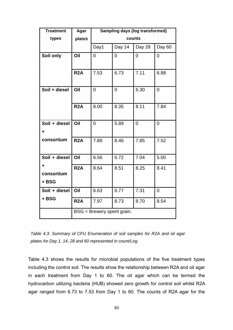
83
Treatment
types
Agar
plates
Sampling days (log transformed)
counts
Day1 Day 14 Day 28 Day 60
Soil only Oil
0 0 0 0
R2A
7.53 6.73 7.11 6.88
Soil + diesel Oil
0 0 6.30 0
R2A
8.00 8.35 8.11 7.84
Soil + diesel
+
consortium
Oil
0 5.89 0 0
R2A
7.89 8.46 7.85 7.52
Soil + diesel
+
consortium
+ BSG
Oil 6.56 6.72 7.04 5.00
R2A 8.64 8.51 8.25 8.41
Soil + diesel
+ BSG
Oil 6.63 6.77 7.31 0
R2A 7.97 8.73 8.70 8.54
BSG = Brewery spent grain.
Table 4.3: Summary of CFU Enumeration of soil samples for R2A and oil agar
plates for Day 1, 14, 28 and 60 represented in count/Log.
Table 4.3 shows the results for microbial populations of the five treatment types
including the control soil. The results show the relationship between R2A and oil agar
in each treatment from Day 1 to 60. The oil agar which can be termed the
hydrocarbon utilizing bacteria (HUB) showed zero growth for control soil whilst R2A
agar ranged from 6.73 to 7.53 from Day 1 to 60. The counts of R2A agar for the

84
treatments with soil and diesel ranged from 7.84 to 8.35 whilst oil agar counts were
only recorded on Day 28. Counts of hydrocarbon degrading bacteria (HUB) in the
treatment with soil plus diesel plus consortium showed a count of 5.89 at Day 14
only and the corresponding R2A agar ranged from 7.52 to 8.46 from Day 1 to 60.
The counts of hydrocarbon utilizing bacteria in soil plus diesel plus consortium plus
BSG ranged from 5.00 to 7.04 and the R2A agar ranged from 8.25 to 8.64 from day
1 to 60 respectively. Whilst that of the treatment with soil plus diesel plus BSG had
counts on R2A ranging from 7.97 to 9.73 and the oil agar ranged from 6.63 to 7.31
from Day 1 to 60 respectively.
Consequently, the counts on contaminated soil were higher than the control soil,
which does not have any BSG or consortium in both R2A and oil agar. Additionally,
the counts on the treatment with BSG were higher than treatment with no BSG.
Treatments with BSG recorded higher counts on both R2A and oil agar than the
treatment with soil and diesel and the consortium.
4.3.3.1 Statistical results of microbial counts
The results from Table 4.4 below indicate that there were differences in microbial
populations between the different soil treatments. Analysis of variance using one-
way ANOVA and a post hoc test to show the differences between the treatment types
for day 1, 14, 28, 42 and 60 were compared with the control soil and the results are
presented in Table 4.4.

85
Data set for p value for day 1 to 60 n=52
Treatment types Soil only for day 1 Soil only for day 14 Soil only for day 28 Soil only for day 60
So + D 0.31 0.01 0.09 0.01
S + D + C 0.64 0.01 0.07 0.13
S + D + C + BSG 0.01 0.01 0.15 0.01
S + D + BSG 0.05 0.01 0.03 0.01
Treatment types Soil + D for day 1 Soil + D for day 14 Soil + D for day 28 Soil + D for day 60
S + D + C 0.55 0.79 0.90 0.24
Soil + D + C +BSG 0.09 0.39 0.85 0.07
Soil + D+ BSG 0.57 0.88 0.42 0.02
Treatment types Soil + D + C for day 1 Soil + D + C for day 14 Soil + D + C for day 28 Soil + D + C for day60
Soil + D + C +BSG 0.01 0.50 0.77 0.01
Soil + D + BSG 0.17 0.91 0.48 0.02
Soil + D + C + BSG 1 Soil + D + C + BSG 14 Soil + D + C + BSG 28 Soil + D + C + BSG60
Soil + D + BSG 0.14 0.46 0.36 0.68
Where= S+D soil+diesel S+D+C soil+diesel+consortium S+D+C+BSG soil+diesel+consortium+BSG
S+D+BSG soil+diesel+BSG
Table 4.4: Results from one-Way ANOVA of microbial counts from day 1 to 60. Post hoc (LSD) a parametric test carried out on treatment with soil only treatment (control), soil plus diesel treatment,
soil plus diesel plus consortium, soil plus diesel plus consortium plus BSG and soil plus diesel plus BSG.

86
Day 1
There was a statistically significant difference between group mean as determined
by one-way ANOVA F (4, 20) = 2.946, p = .046. Post hoc (LSD) test revealed that
treatment with soil only (control) was significantly lower in microbial populations (M =
7.48 SD = 0.53 SE = 0.20) compared to treatment with soil plus diesel plus
consortium plus BSG (M = 8.90 SD = 0.38 SE = 0.22), p = 0.005 and treatment with
soil plus diesel plus BSG (M = 8.21 SD = 0.57 SE = 0.21), p = 0.051. However,
There was no statistically significant difference between treatment with soil only
(control) and treatment with soil plus diesel p = 0.312 and treatment with soil plus
diesel plus consortium p = 0.640.
Day 14
There was a statistically significant difference between group mean as determined
by one-way ANOVA F (4, 14) = 11.102, p = 0.001). Post hoc (LSD) test revealed that
bacteria numbers for the treatment with soil only (control) was significantly different
(M = 6.72 SD = 0.08 SE = 0.08) as compared to the treatment with soil plus diesel
(M = 8.41 SD 0.25 SE = 0.13), p = 0.001 and treatment with soil plus diesel plus
consortium plus BSG (M = 8. 70 SD 0.68 SE = 0.39), p = 0.001 and also treatment
with soil plus diesel plus consortium (M = 8.49 SD 0.38 SE = 0.17) , p = 0.001.
Day 28
There was no statistically significant difference between group mean as determined
by one-way ANOVA F (4, 12) = 1.677, p =0 .219). Post hoc (LSD) test revealed that
treatment with soil only (Control) was not statistically different in microbial
populations from treatment with soil plus diesel p = 0.095 and treatment with soil plus
diesel plus consortium p = 0.079 and treatment with soil plus diesel plus consortium
plus BSG p = 0.153. However, the treatment with soil only was significantly lower (M
= 7.06 SD = 0.18 SE = 0.11) compared to the treatment with soil plus diesel plus
BSG (M = 8.47 SD 0.42 SE = 0.42), p = 0.030.

87
Day 60
There was a statistically significant difference between group mean as determined
by one-way ANOVA F (4, 24) = 7.490, p =0 .001. Post hoc (LSD) test revealed that
the treatment with soil only was significantly lower in microbial populations (M = 7.00
SD = 0.25 SE = 0.12) compared to the treatment with soil plus diesel (M = 7.86 SD
= 0.89 SE = 0.34), p = 0.014 and treatment with soil plus diesel plus consortium plus
BSG (M = 8.40 SD = 0.28 SE = 0.11), p = 0.001 and treatment with soil plus diesel
plus BSG (M = 8.53 SD = 0.36 SE = 0.15), p = 0.001. However, there was no
statistically significant difference in microbial populations between soil only (control)
and treatment with soil plus diesel plus consortium p = 0.137. Details of the ANOVA
table and post hoc test are shown above in Table 4.4 above.

88
The soil pH changed little throughout the experiment. At the beginning of the
experiment the control soil had a pH of 6.7 and at day 42 it was 6.4 the pH taken at
day 60 was 6.5. The treated soil plus diesel had an initial pH of 5.8 which rose to 6.4
at day 28. This further increased to 6.9 at days 42 and 60 respectively. Similarly, the
treated soil plus diesel plus consortium had an initial pH of 5.9 which rose to 6.4 at
day 28 increasing to 6.9 at day 42 but dropping to 6.7 at day 60.
The treated soil plus diesel plus consortium plus BSG had an initial pH of 6.3 which
rose to 7.0 at day 28 and dropped to 6.6 at days 42 and 60 respectively. In a similar
pattern the treated soil plus diesel plus BSG also had an initial pH of 6.2 which rose
to 7.1 at day 28 but began to drop at days 42 and 60 to 6.9 and 6.6 respectively.

89
The average experimental temperatures recorded also changed throughout the
duration of the experiment ranging from 180C at day 1, to 220C at day 42 increasing
to 250C at day 60. The temperature was not control and could be regarded as warm
throughout the duration of the experiment.
4.4 Methods
Experiment (b)
This study was carried out to determine the biodegradation of diesel in soil to which
1% (v/w) of diesel had been added with/without the addition of 10% BSG. The aim of
this experiment was to further investigate the use of BSG in the bioremediation
process. In order to achieve this two treatments were investigated - treatment with
BSG and treatment without BSG. The amount of diesel used in each tray in this
experiment was 10,000 mg kg-1soil and experiment (a) was 5,000 mg kg-1soil. The
percentage of diesel added to the soil in experiment (b) was 1% compared to 0.5%
in experiment (a). The methods and materials used are described in the next section.
4.4.1 Method of experiment (b)
The materials used in the study are described in section 3.2.1, 3.2.2 and 3.2.3. Table
4.6 shows the composition of the treatments and how they were applied in the study.

90
From table 4.6 Treatment (1) contains 2 kg of soil only, which is the control sample
without BSG and treatment (2) contains 2 kg of soil which was contaminated with 1%
diesel (v/w). The composition of treatment (3) was the addition of 1% diesel to 2 kg
of soil plus 200 g BSG (w/w). Treatment (4) contains 2 kg of soil and 200 g BSG. The
diesel and BSG were added to the soil treatments according to the method detailed
in section 3.7.2. A photograph of the soil and trays is shown Fig.4.3.
Treatment types % of diesel in
the soil
Grams of soil
+ diesel
BSG
(10%)
added in
grams
Number of
trays
1 -
2000
-
3
2
1%
2000
-
3
3
1%
2000
200
3
4 -
2000
200
3
Table 4.6: Composition of the different treatments incubated in the laboratory
including soil only treatment (control), soil plus diesel (10,000 mg kg-1 soil), soil
plus diesel (10,000 mg kg-1) plus 200 g brewery spent grain and soil plus 200 g
brewery spent grain (control)
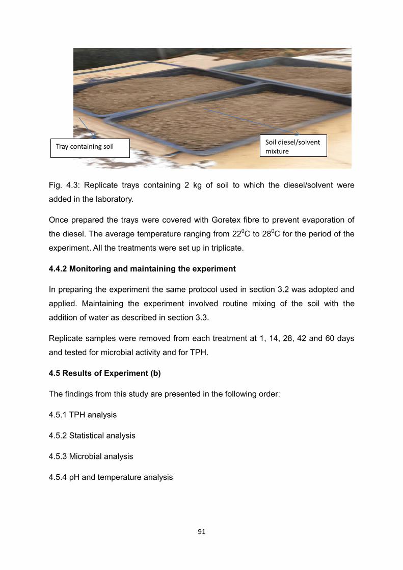
91
Fig. 4.3: Replicate trays containing 2 kg of soil to which the diesel/solvent were
added in the laboratory.
Once prepared the trays were covered with Goretex fibre to prevent evaporation of
the diesel. The average temperature ranging from 220C to 280C for the period of the
experiment. All the treatments were set up in triplicate.
4.4.2 Monitoring and maintaining the experiment
In preparing the experiment the same protocol used in section 3.2 was adopted and
applied. Maintaining the experiment involved routine mixing of the soil with the
addition of water as described in section 3.3.
Replicate samples were removed from each treatment at 1, 14, 28, 42 and 60 days
and tested for microbial activity and for TPH.
4.5 Results of Experiment (b)
The findings from this study are presented in the following order:
4.5.1 TPH analysis
4.5.2 Statistical analysis
4.5.3 Microbial analysis
4.5.4 pH and temperature analysis
Soil diesel/solvent mixture
Tray containing soil Soil diesel/solvent mixture
Tray containing soil
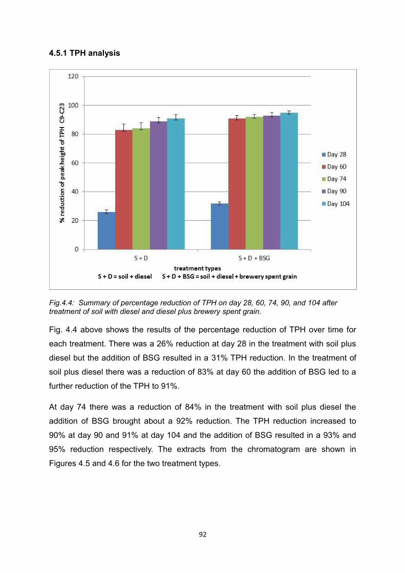
92
4.5.1 TPH analysis
Fig.4.4: Summary of percentage reduction of TPH on day 28, 60, 74, 90, and 104 after treatment of soil with diesel and diesel plus brewery spent grain.
Fig. 4.4 above shows the results of the percentage reduction of TPH over time for
each treatment. There was a 26% reduction at day 28 in the treatment with soil plus
diesel but the addition of BSG resulted in a 31% TPH reduction. In the treatment of
soil plus diesel there was a reduction of 83% at day 60 the addition of BSG led to a
further reduction of the TPH to 91%.
At day 74 there was a reduction of 84% in the treatment with soil plus diesel the
addition of BSG brought about a 92% reduction. The TPH reduction increased to
90% at day 90 and 91% at day 104 and the addition of BSG resulted in a 93% and
95% reduction respectively. The extracts from the chromatogram are shown in
Figures 4.5 and 4.6 for the two treatment types.

93
Fig 4.5: Extract from chromatogram for day 1, day 60 and day 90 for soil plus diesel showing
the degradation of the diesel over time.
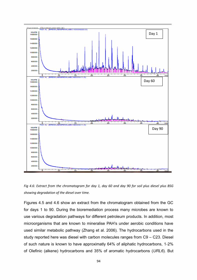
94
Fig 4.6: Extract from the chromatogram for day 1, day 60 and day 90 for soil plus diesel plus BSG
showing degradation of the diesel over time.
Figures 4.5 and 4.6 show an extract from the chromatogram obtained from the GC
for days 1 to 90. During the bioremediation process many microbes are known to
use various degradation pathways for different petroleum products. In addition, most
microorganisms that are known to mineralise PAH’s under aerobic conditions have
used similar metabolic pathway (Zhang et al. 2006). The hydrocarbons used in the
study reported here was diesel with carbon molecules ranges from C9 – C23. Diesel
of such nature is known to have approximatly 64% of aliphatic hydrocarbons, 1-2%
of Olefinic (alkene) hydrocarbons and 35% of aromatic hydrocarbons (URL6). But
Fig 4.4: Extract from chromatogram for day1, day 60 and day 90 for soil plus diesel plus brewery
spent grain showing degradation of diesel over time.
Day 1
Day 60
Day 90
95
hydrocarbons have a different degree of susceptibility to microbial attack. The order
of such decreasing susceptibility are n-alkanes > branched alkanes > aromatic of low
molecule weight > cyclic alkanes (Perry, 1984).
Figures 4.5 and 4.6 show the reduction patterns of the diesel compounds with the
high molecular weights expected to take a longer time to degrade. The light fractions
are expected to degrade within the early stage of bioremediation (Bento, et al. 2005).
In the study reported here it was observed in the GC monitoring that there was an
increase in the number of low molecular weights hydrocarbons within 28 days of the
experiment suggesting that the higher molecular weights were broken down,
resulting in an increased number of lower molecular weights hydrocarbons. The
increase in the number was qualitatively observed to be greater in soil treated with
BSG than soil without BSG. This study characterised the hydrocarbon degrading
bacteria responsible for degrading diesel contaminated soil using oil agar and
measured the total TPH using the peak height, each of the hydrocarbon constituents
were not identified. As such further studies are needed to determine if the increase in
low molecular weights hydrocarbons was as a result of the addition of the BSG used
to augment the bioremediation process.
The highest percentage of reduction in peak height was observed within 28 days of
the experiment part of this may be attributed to volatilisation and microbial attack on
the diesel compounds as reported in (Bento, et al. 2005). More so, from the results
of the soil microbiological enumeration presented in the study, it may be inferred that
the high percentage of diesel-degrading microorganisms indicates that there are
more heterotrophic microorganisms in the soil treated with BSG than soil without
BSG suggesting the population of oil degrading microorganisms influenced the
degradation process. According to Salminen (2004) in order for the products of the
tri-carboxylic acid TCA cycle (amino acids, protein, nucleotides and nucleic acids) to
be synthesised, a nitrogen, sulphur and phosphorous source is required, in the study
reported here BSG was added as a nutrient in the bioremediation process. The end
processes of respiration are CO2, water and the cell biomass (Salminen, (2004).
The reduction pattern for both treatment types has previously been presented as
percentages. At day 104 the treatment with soil plus diesel resulted in 91%
degradation and the introduction of BSG brought about a further reduction to 95%.

96
The statistical analysis carried out on the original data showed that there was a
statistically significant difference between the treatment with soil plus diesel and
treatment with soil plus diesel plus BSG p = 0.05.

97
4.5.2 Statistical results for TPH
The results from Table 4.7 indicate that there were differences in the TPH reduction in the various treatment types. Independent t-
test (parametric) and Mann-Whitney U statistical tests were conducted on the data to show the differences between the treatment
types for day 1, 28, 60, 74, 90 and 104. The reason for conducting the two tests was for the results to be compared and to gain
extra confidence from the conclusions that could be drawn.
Statistical Test Data set Day
1
Data set for Day 28
Data set for Day 60
Data set Day
74
Data set Day
90
Data set Day 104
Mann-Whitney U test (Non-
parametric)
0.41 0.16 0.01 0.01 0.78 0.01
Independent t-test(parametric) 0.41 0.13 0.01 0.01 0.06 0.01
Sample Size n= 36 n= 36 n=36 n=36 n=36 n=36
Where * = significant difference
Table 4.7:Results of TPH from Mann Whitney non-parametric test and a parametric independent t-test, carried out on soil plus diesel treatment
data and soil plus diesel plus BSG data on day 1, 28, 60, 74, 90 and 104.

98
Independent t-test (parametric)
Day 1
An independent-sample t-test indicated that there was no significant difference
between the total peak height for the treatment of soil plus diesel (M = 157, SD = 83)
compared to the treatment with soil plus diesel plus BSG (M = 135, SD = 78 ), t(34),
0.817, p = 0.419.
Day 28
An independent-sample t-test indicated that there was no significant difference
between the total peak height for the treatment of soil plus diesel (M = 119, SD = 60)
compared to the treatment with soil plus diesel plus BSG (M = 92, SD = 42), t (34)
1.528, p = 0.136.
Day 60
An independent-sample t-test indicated that the total peak height was statistically
higher in the treatment with soil plus diesel (M = 27, SD = 18) compared to the
treatment with soil plus diesel plus BSG (M = 12, SD = 8), t (24) 3.129, p = 0.005.
Day 74
An independent-sample t-test indicated that the total peak height was significantly
higher in the treatment with soil plus diesel (M = 24, SD = 16) compared to the
treatment with soil plus diesel BSG (M = 11, SD = 7), t (23) 3.272, p = 0.003.
Day 90
An independent-sample t-test indicated that there was no statistically significant
difference between the total peak height for the treatment with soil plus diesel (M =
15, SD = 11) compared to the treatment with soil plus diesel plus BSG (M = 9, SD =
8), t (34) 1.943, p = 0.060.
Day 104
An independent-sample t-test indicated that the total peak height was significantly

99
higher in the treatment with soil plus diesel (M = 14, SD = 11) compared to the
treatment with soil plus diesel plus BSG (M = 6, SD = 5), t (24) 2.628, p =0.015.
Detailed results of the independent t-test can be found in table 4.6 above.
Mann-Whitney U test (non-parametric)
A Mann-Whitney U test was conducted for all of the data across each day and
between the two treatment types. It revealed that :
Day 1
There was no statistically significant difference between the total peak height for
treatment with soil plus diesel (Mdn = 150, n = 36) compared to treatment with soil
plus diesel plus BSG (Mdn =135, n = 36), U = .136, z = 0.14, p = 0.411.
Day 28
There was no statistical significant difference between the total peak height for
treatment with soil plus diesel (Mdn = 120, n = 36) compared to treatment with soil
plus diesel plus BSG (Mdn =93, n = 36), U = .118, z = 0.232, p = 0.164
Day 60
A Mann-Whitney U test indicated that the treatment with soil plus diesel was
significantly higher in total peak height (Mdn = 28, n = 36) compared to the treatment
with soil plus diesel plus BSG (Mdn = 13, n = 36), U = .79, z = 0.44, p = 0.009.
Day 74
A Mann-Whitney U test indicated that the treatment with soil plus diesel was
significantly higher in total peak height (Mdn = 26, n = 36) compared to treatment
with soil plus diesel plus BSG (Mdn = 11, n = 36), U = .80, z = 0.43, p = 0.009.
Day 90
There was no statistically significant difference between the total peak height for
treatment with soil plus diesel (Mdn = 18, n = 36) compared to treatment with soil
plus diesel plus BSG (Mdn =8, n = 36), U = .107, z = 0.29, p = 0.078.
100
Day 104
A Mann-Whitney U test indicated that the treatment with soil plus diesel was
significantly higher in total peak height (Mdn = 13, n = 36) compared to treatment
with soil plus diesel plus BSG (Mdn = 5, n = 36), U = .94, z = 0.36, p = .031. Detailed
results of the Mann-Whitney U test can be found in table 4.7 above.
4.5.3 Microbial analysis
4.5.3.1 CFU Enumeration
The microbial populations of the various soil samples were enumerated based on the
two Agar plates (R2A and oil) over 90 days (Day 1, 14, 24, 56, 70 and 90). The R2A
agar is a general representation of the microbial populations and the oil agar should
indicate those bacteria capable of using diesel as a substrate. The results of R2A
and Oil agar are reported in Table 4.7 below in their respective log form.
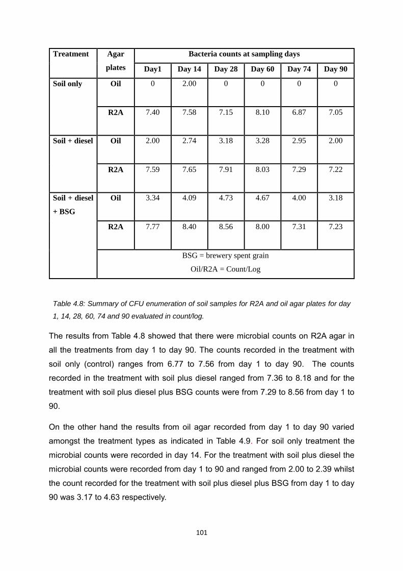
101
The results from Table 4.8 showed that there were microbial counts on R2A agar in
all the treatments from day 1 to day 90. The counts recorded in the treatment with
soil only (control) ranges from 6.77 to 7.56 from day 1 to day 90. The counts
recorded in the treatment with soil plus diesel ranged from 7.36 to 8.18 and for the
treatment with soil plus diesel plus BSG counts were from 7.29 to 8.56 from day 1 to
90.
On the other hand the results from oil agar recorded from day 1 to day 90 varied
amongst the treatment types as indicated in Table 4.9. For soil only treatment the
microbial counts were recorded in day 14. For the treatment with soil plus diesel the
microbial counts were recorded from day 1 to 90 and ranged from 2.00 to 2.39 whilst
the count recorded for the treatment with soil plus diesel plus BSG from day 1 to day
90 was 3.17 to 4.63 respectively.
Treatment Agar
plates
Bacteria counts at sampling days
Day1 Day 14 Day 28 Day 60 Day 74 Day 90
Soil only Oil
0 2.00 0 0 0 0
R2A
7.40 7.58 7.15 8.10 6.87 7.05
Soil + diesel Oil
2.00 2.74 3.18 3.28 2.95 2.00
R2A
7.59 7.65 7.91 8.03 7.29 7.22
Soil + diesel
+ BSG
Oil
3.34 4.09 4.73 4.67 4.00 3.18
R2A
7.77 8.40 8.56 8.00 7.31 7.23
BSG = brewery spent grain
Oil/R2A = Count/Log
Table 4.8: Summary of CFU enumeration of soil samples for R2A and oil agar plates for day
1, 14, 28, 60, 74 and 90 evaluated in count/log.

102
4.5.3.2 Statistical analysis of microbial populations
The results from Table 4.9 indicate that there were differences in microbial
populations between the different soil treatments. Analysis of variance using one-
way ANOVA and post hoc test to show the differences between the treatment types
for day 1, 14, 28, 42, 60, 74 and 90 and compared with the control soil are presented
below in Table 4.9.
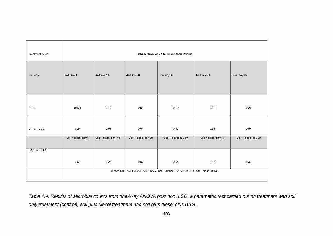
103
Treatment types
Data set from day 1 to 90 and their P value
Soil only
Soil day 1
Soil day 14
Soil day 28
Soil day 60
Soil day 74
Soil day 90
S + D
0.631
0.10
0.01
0.19
0.12
0.26
S + D + BSG
0.27
0.01
0.01
0.33
0.51
0.84
Soil + diesel day 1 Soil + diesel day 14 Soil + diesel day 28 Soil + diesel day 60 Soil + diesel day 74 Soil + diesel day 90
Soil + D + BSG
0.58
0.28
0.07
0.64
0.33
0.36
Where S+D soil + diesel S+D+BSG soil + diesel + BSG S+D+BSG soil +diesel +BSG
Table 4.9: Results of Microbial counts from one-Way ANOVA post hoc (LSD) a parametric test carried out on treatment with soil
only treatment (control), soil plus diesel treatment and soil plus diesel plus BSG.

104
Day 1
There was no statistically significant difference between group means as determined
by one-way ANOVA F(2,16) = 0.651, p = 0.535. Post hoc (LSD) test revealed that the
microbial population was not significantly higher in the treatment with soil only as
compared to the treatment with soil plus diesel p = 0.631 and treatment with soil plus
diesel plus p = 0.272. There were no significant differences in microbial populations
between the treatment with soil plus diesel plus BSG and the treatment with soil plus
diesel p = 0.586.
Day 14
There was a statistically significant difference between group mean as determined
by one-way ANOVA F(2,15) = 4.140, p = 0.037. Post hoc (LSD) test revealed that the
microbial populations in the treatment with soil only (control) was significantly lower
(M= 7.47 SD = 0.51 SE = 0.21) as compared to the treatment with soil plus diesel
plus BSG (M = 8.31 SD = 0.61 SE = 0.25), p = 0.012. However, there was no
statistically significant difference between the treatment with soil plus diesel,
treatment with soil only p = 0.103 and treatment with soil plus diesel plus BSG p =
0.281.
Day 28
There was a statistically significant difference between the group mean as
determined by one-way ANOVA F (2, 14) = 9.029, p = 0.003. Post hoc (LSD) test
revealed that the microbial populations in the treatment with soil only (control) was
significantly lower (M = 7.24 SD = 0.25 SE = 0.11) compared to treatment with soil
plus diesel (M = 8.01 SD = 0.60 SE = 0.21), p = 0.013 and treatment with soil plus
diesel plus BSG (M = 8.57 SD = 0.33 SE = 0.16), p = 0.001. However, there was no
significant difference between the treatment with soil plus diesel plus BSG and the
treatment with soil plus diesel p = 0.071.
Day 60
There was no statistically significant difference between group means as determined
by one-way ANOVA F (2,13) = 1.033, p = 0.384. Post hoc (LSD) test revealed that
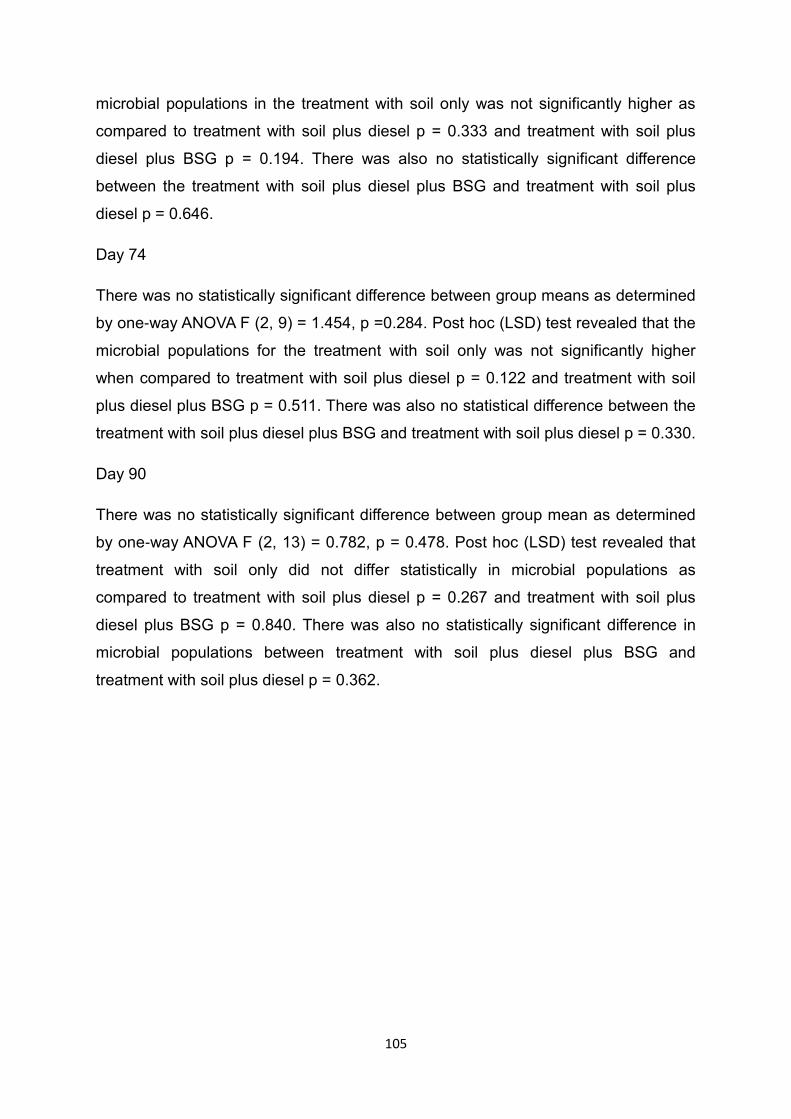
105
microbial populations in the treatment with soil only was not significantly higher as
compared to treatment with soil plus diesel p = 0.333 and treatment with soil plus
diesel plus BSG p = 0.194. There was also no statistically significant difference
between the treatment with soil plus diesel plus BSG and treatment with soil plus
diesel p = 0.646.
Day 74
There was no statistically significant difference between group means as determined
by one-way ANOVA F (2, 9) = 1.454, p =0.284. Post hoc (LSD) test revealed that the
microbial populations for the treatment with soil only was not significantly higher
when compared to treatment with soil plus diesel p = 0.122 and treatment with soil
plus diesel plus BSG p = 0.511. There was also no statistical difference between the
treatment with soil plus diesel plus BSG and treatment with soil plus diesel p = 0.330.
Day 90
There was no statistically significant difference between group mean as determined
by one-way ANOVA F (2, 13) = 0.782, p = 0.478. Post hoc (LSD) test revealed that
treatment with soil only did not differ statistically in microbial populations as
compared to treatment with soil plus diesel p = 0.267 and treatment with soil plus
diesel plus BSG p = 0.840. There was also no statistically significant difference in
microbial populations between treatment with soil plus diesel plus BSG and
treatment with soil plus diesel p = 0.362.
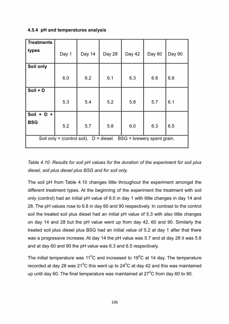
106
4.5.4 pH and temperatures analysis
Treatments
types
Day 1
Day 14
Day 28
Day 42
Day 60
Day 90
Soil only
6.0
6.2
6.1
6.3
6.8
6.8
Soil + D
5.3
5.4
5.2
5.8
5.7
6.1
Soil + D +
BSG
5.2
5.7
5.8
6.0
6.3
6.5
Soil only = (control soil). D = diesel. BSG = brewery spent grain.
Table 4.10: Results for soil pH values for the duration of the experiment for soil plus
diesel, soil plus diesel plus BSG and for soil only.
The soil pH from Table 4.10 changes little throughout the experiment amongst the
different treatment types. At the beginning of the experiment the treatment with soil
only (control) had an initial pH value of 6.0 in day 1 with little changes in day 14 and
28. The pH values rose to 6.8 in day 60 and 90 respectively. In contrast to the control
soil the treated soil plus diesel had an initial pH value of 5.3 with also little changes
on day 14 and 28 but the pH value went up from day 42, 60 and 90. Similarly the
treated soil plus diesel plus BSG had an initial value of 5.2 at day 1 after that there
was a progressive increase. At day 14 the pH value was 5.7 and at day 28 it was 5.8
and at day 60 and 90 the pH value was 6.3 and 6.5 respectively.
The initial temperature was 110C and increased to 190C at 14 day. The temperature
recorded at day 28 was 210C this went up to 240C at day 42 and this was maintained
up until day 60. The final temperature was maintained at 270C from day 60 to 90.

107
4.6 Discussion
The measurement of hydrocarbon degradation can be assessed using both chemical
and biological methods (CL:AIRE, 2006 and EA, 2010b), however effective
bioremediation cannot be measured using a single parameter. Several methods
used to assess microbial activities have provided a meaningful method of
characterising microbial communities during bioremediation. These include microbial
enumeration, soil respiration and enzyme activity such as dehydrogenase,
phosphate assay and proteases (Margesin, 2000). Measures such as microbial
biomass and enzyme activity could be seen as a possible means of evaluating the
healthy nature of the soil and the potential success of bioremediation (Dick and
Tabatabai, 1992). Dadrasnia and Agamuthu (2010) used microbial enumeration to
evaluate the bioremediation of diesel-contaminated soil, where organic wastes were
applied to augment the bioremediation process. Jorgensen et al.(2000) measured
microbial activity by measuring soil respiration for composting of contaminated soil in
biopiles in an ex-situ technology. Here organic matter, such as bark chips was added
to the contaminated soil as a bulking agent.
The committee of In Situ bioremediation has recommended strategies for evaluating
progress of bioremediation (EA, 2010a), these include: documented loss of
contaminants from the site, laboratory assays which should show that the
microorganisms from the site have the potential to transform the contaminants,
under the expected conditions at the site. One or more pieces of information should
demonstrate that biodegradation potentials can actually be realised in the field (EA,
2010b). TPH could be evaluated to determine the relative concentration of petroleum
in the soil. TPH may be recorded as mg/kg, ppm or as a relative percentage of the
total sample (U.S DOE, 1996).
Therefore, the purpose of this section is to discuss the results obtained from the
laboratory experiments on different bioremediation processes in addition to their
biological activities with regard to their usefulness for monitoring and for assessing
the results of the soil experimentally contaminated with diesel. Changes in diesel
concentration and the accompanying changes in microbial activities with time were
measured.

108
4.6.1 Microbial analysis
The composition of microbial populations in soils at contaminated sites can be
affected by the composition of the hydrocarbons in the soil (Admon, 2001). Addition
of diesel to soils provides a source of carbon for any micro-organisms present, but
the resultant increase in carbon may lead to an imbalance of nitrogen and
phosphorus, which may prove to inhibit microbial activities (Morgan and Watkinson,
1989 and Kim, 2005). Nitrogen and phosphorous can then be a limiting factor in the
bioremediation of hydrocarbon contaminated soils (Yang et al. 2009).
In the study presented here the plate count method was used to quantify the
population and activity of the soil micro-organisms and the technique used evaluated
the number of microbes (R2A) and their biodegradation potentials as measured by
their growth on oil agar. The results of the microbial counts, using R2A agar showed
there was a higher count in the soils with diesel and soil with BSG than the control
soil as indicated in both experiments. The statistical analysis showed that the control
soil was significantly lower than treated soil plus diesel and treatment with BSG p =
0.05. Although in experiment (b) there were lower microbial counts for R2A plates
in the control soil compared to the treatment with soil plus diesel and treatment with
BSG but there was no significant difference between these treatments except on
days 14 and 28 p = 0.05. However, the differences between the treatments in both
experiments could be due to the inherent heterogeneity of the mixture of soil
samples after the addition of BSG or the addition of consortium as indicated in Table
4.1 and Table 4.6.
The increase in microbial counts in R2A agar for soil with diesel and treatment with
amendment is expected because higher amounts of electron donors (from the
hydrocarbon substrate) can support larger populations of microorganisms. This
coupled with the addition of BSG which may bring additional bacteria, may also
explain the higher microbial counts with treatment with BSG. In determining the
possibility of bioremediation in hydrocarbon contaminated soil, the U.S EPA (United
States Environmental Protection Agency) suggests that there should be 10 x 103
colony forming units per gram of soil in contaminated soil (Ta – Chen, 2010). In the
present study the colony forming unit per gram of soil for both experiments exceeded
this threshold.
109
However, there are limitations to the use of plate count methods to quantify the
population and activity of soil microorganism in the study. This means increased
numbers of microorganisms in a particular treatment should not be assumed to
indicate the presence of microbes that can degrade the contaminants present or as
strong evidence of bioremediation occurring. Using R2A agar plate counts could be
misleading because of the thousands of different bacterial species in one gram of
soil of which less than 1% could be culturable (Rossello-Mora and Amann, 2001).
Besides, R2A agar contains simple sugars and is likely to grow those micro-
organisms unable to digest hydrocarbons. This means that R2A agar will only give a
general representation of the microbial populations of the soil. All these factors could
contribute to the varied cell counts found, in the sample, in this study.
However, the detection of microbial activities using oil media with hydrocarbons as a
carbon source could be used to determine the presence of hydrocarbon degrading
bacteria as reported by (Dadrasnia and Agamuthu, 2010). Hence the results
obtained with this media were used to evaluate the biodegradation potentials of the
bacteria in the diesel contaminated soil. These hydrocarbon degrading bacteria were
comparable to the R2A agar in all the treatment types. The difference between the
two media in each treatment type could be attributed to the richness in microbial
activities of the treatment with BSG and a lack of sufficient nutrients in the treatment
without BSG.
An analysis of the data in Table 4.3 and 4.8 shows that the growth rates of R2A and
oil agar were higher in treatments with BSG compared to treatments without BSG
experiments (a) and (b) respectively. In the present study the reasons attributed to
higher counts of bacteria in R2A and oil agar in soil with BSG could be due to the
presence of considerable quantities of nitrogen and phosphorus in the soil with BSG,
which are requisite nutrients for bacteria/ biodegradative activities (Adesodun and
Mbagwu, 2008).
BSG is a beverage industry by-product having food characteristics, it is used in
agriculture because of its high organic matter and is known to contain significant
energy resources from its organic content (Thomas and Rahman, 2006) and soil
organic matter content and biomass are related to microbial activities (Garcia-Gill,
2000). The BSG may provide organic material suitable for bacterial growth and the
110
growth on R2A media may not be indicative of bacterial that are breaking down the
diesel however, the growth found on the oil media had diesel as a source of carbon,
so bacterial growth here is indicative of those that can breakdown diesel.
In addition, the results of microbial counts in the two experiments showed that
microorganisms capable of using the diesel as a nutrient source were only isolated
from the contaminated soil with diesel and soil treated with diesel and BSG. These
organisms were rarely found in soil without hydrocarbon or treatment without
amendment. In experiment (a) the presence of the microbes were lowered across
the treatment types but in experiment (b) the microbes were dominant in all the
treatment types except the control soil. The difference between the two experiments
was due to the dilution series adopted in the study, as dilution series for experiment
(a) was 10-4 to 10-6 and experiment (b) was 10-2 to 10-4 . The dilution series with 10-4
to 10-6 recorded few or no counts in some treatments as shown in the results
section. Therefore, an increase in dilution series in experiment (b) resulted in a high
concentration of micro-organisms with the treatment, with BSG having higher
concentrations in both R2A and oil agar compared to treatment without BSG.
4.6.2 pH values and temperature
Hydrocarbon degrading bacteria are known to be sensitive to pH in the soil, which
may depend on biotic factors such as nutrients and water (Margesin and Schinner,
2001). The optimum pH value for oil degradation is 6.5 to 8.0 and the condition
required for microbial activities to thrive is between 5.5 to 8.8 (Vidali, 2001). Thus,
similar values were observed in all the soil samples during the bioremediation
process in experiments (a) and (b), except in the initial stage of the treatment in
experiment (b) where the addition of the diesel had a slight effect on soil pH. Soils
affected by crude oil are expected to have a lower pH value than similar unaffected
soils. The reason for low pH is that hydrocarbons may be expected to have free
cations giving them the properties of a weak acid (U.S DOE, 1996). However, the
addition of BSG and other factors such as temperature were seen to raise the pH
level. This suggests that BSG enhances the compounds that neutralise the acidity of
the soil brought about by the diesel contamination as reported by U.S DOE (1996).
Changes in temperatures are known to affect the utilization of substrate within
hydrocarbon mixtures (Mittal and Singh, 2009) and also temperature changes the

111
rate of carbon mineralization, through the reduction of alternative electron acceptors
(Van Hulzen, 1999). The temperature required for microbial activities range from 14
to 310C and the optimum value of temperature for oil degradation is 200C to 300C
(Vidali, 2001). A similar temperature was recorded in both experiments with a slight
variation at the beginning of the experiment as indicated in section 4.3.4 and 4.5.5.
The temperature condition in the study could be regarded as warm, which is known
to favour biologically driven degradation of compounds such as hydrocarbons (CL:
AIRE, 2007).
More so, microbes that are known to degrade hydrocarbons needs oxygen to
survive, in the study oxygen levels were not measured directly but a sufficient level
of soil aeration was achieved by turning the soil and the moisture content was
maintained accordingly. Thus, turning the soil enables the diesel and the soil/BSG
mixture to mix and be evenly distributed, as expected this enhances the process by
providing an enabling environment for the microbe colonies to have viable contact
with food and nutrients. Hence in these experiments conditions were optimised
which is something that may not happen in the field where environmental conditions
may impact on the success of achieving a bioremediation target. It has been
reported that bioremediation was delayed at a site in the U.S. by high moisture
conditions due to unseasonably wet weather from November 1995, until June 1996
and soil temperature below 50C or above 320C could retard or stop microbial
processes (U.S. DOE, 1996).
In the study here a consistent volume of water was added to the soil to maintain the
experiment and in all cases this was 85 cms3 for treatment without BSG and 176
cms3 for treatment with BSG in 1000 g of soil, which is less than the field water
holding capacity. The level of water added showed that the soil was moist but not
waterlogged and because water was added twice weekly, in addition to turning the
soil, the bacteria in the soil were expected to have a viable contact with the
contaminants. However, the use of sufficient water to meet the water holding
capacity and maintaining all environmental conditions may further enhance the
breakdown of the diesel contaminants. Further studies are needed to demonstrate
the practicality of the technique under field condition.
112
4.6.3 Total petroleum hydrocarbon (TPH)
Petroleum hydrocarbons such as diesel can be identified and quantified by
comparing sample chromatograms with calibration of the gas chromatograph with
diesel. Bento, (2005) calculated the percentage degradation of diesel oil as (TPH
control – TPH treatment/TPH control x 100) and the initial hydrocarbon values
establish the baseline or the starting point for a bioremediation project (U.S. DOE,
1996).
In the present study the progress of bioremediation was measured by calculating
the percentage degradation of the diesel contaminated soil by measuring the total
peak height and this was achieved by obtaining the initial hydrocarbon value, which
served as the starting point and measuring it with the progress of the bioremediation
process up to the last day of the experiment. From both experiments in Fig 4.1 and
4.2 there was an increasing reduction in the TPH using the total peak height in all
treatments with BSG/consortium and treatments without BSG. There are
disadvantages of using the total peak because it is difficult to determine the mass of
carbon, however, it could be used to calculate the percentage degradation and
compared to the extract from the chromatogram to show if degradation actually
occurred.
In the study here percentage reduction of total peak height was used for the amount
of diesel in the soil. Initially it has been evaluated that 68% of diesel can be
recovered from the soil according to the method in section 3.7.2 and Fig.3.4. This is
the amount of diesel that can be recovered in the soil when a given amount is added.
The initial soil concentrations of the diesel were 5,000 mg kg-1 and 10,000 mg kg-1
for experiment (a) and (b) (Table 4.1 and 4.6), however, given the 68% recovery
level the measurable concentration of diesel in the soil for experiments (a) and (b)
were 3,400 mg kg-1 and 6,800 mg kg-1 respectively. To this end the percentage
reduction and the degradation were based on these concentration levels for both
experiments.
In experiment (a) TPH reduction was measured by the total peak height in all the
treatment types from day 14, 28, 42 and 60. This was calculated as percentage
degradation as shown in Figure 4.1. The percentage degradation from experiment
(a) showed that at day 60 the treatment with soil plus diesel recorded 72%

113
degradation and the addition of consortium resulted in 83% degradation while the
addition of BSG resulted to further degradation of 95%. In experiment (b) TPH
reduction was also calculated as percentage degradation and reduction was
observed in all treatments at day 28, 42, 60, 74, 90 and 104 as indicated in Figure
4.2. The qualitative observation of the chromatogram for treated soil plus diesel and
treated soil plus diesel plus BSG are shown in Figure.4.3 and Figure 4.4 in the
results section shows that the lower molecular weight molecules breakdown more
quickly than those with a high molecular weight, which are considered to be
recalcitrant. The treatment with soil plus diesel plus BSG resulted in 95%
degradation. The statistical analysis for both treatments showed that there was a
significant difference between the treated soil with BSG and treated soil without BSG
p = 0.05.
The results from experiment (a) and (b) showed the effective bioremediation of
petroleum contamination. This is contrary to the study of Bento et al. (2005) which
carried out a comparative evaluation of soil contaminated with diesel collected from
Long Beach, California, USA and Hong Kong and China. The three technologies of
natural attenuation, biostimulation and bioaugmentation were evaluated. Natural
attenuation was the ability of the microbes present in the soil to degrade the
contaminants. Whilst biostimulation involved the addition of (NH4)2 and K2HPO4 and
bioaugmentation was the addition of a microbial consortium from selected species
isolated from a contaminated soil.
After 12 weeks of incubation all three treatment types showed different effects on
the degradation of TPH with bioaugmentation showing the greatest degradation in
Long beach soil and Hong Kong soil. Natural attenuation was more effective than
biostimuation (addition of nutrients). The light fraction (C12 – C23) degradation using
bioaugmentation in the Long Beach soil was 75% and biostimulation and natural
attenuation were 46% and 49% respectively. Whilst in the Hong Kong study, soil
bioaugmentation was 73% and biostimulation and natural attenuation were 45% and
46% accordingly.
In the present study biostimulation (addition of BSG) in experiment (a) was more
effective than bioaugmentation (addition of consortium) which was a treatment
without BSG. The reasons for this could be attributed to different conditions and

114
experimental design as the hydrocarbon degrading bacteria consortium used by
Bento et al. (2005) were those previously isolated from Long Beach, California. In
the present experiment the bacterial consortium used was obtained from Teesside
University and was known to be hydrocarbon degrading bacteria and the soil was a
spiked soil as compared to contaminated diesel oil obtained from the field.
In the results reported here the BSG may optimise the conditions by the addition of
organic nutrients as suggested by Dadrasnia and Agamuthu, (2013). In the study
reported by Dadrasnia and Agamuthu, (2013) tea leaf, soy cake, and potato skin
were used to augment the bioremediation of soil spiked with diesel for a period of 3
months in the laboratory. Their findings showed that hydrocarbon utilizing bacteria
were more abundant in the diesel polluted soil amended with different organic
wastes than of the unamended polluted soil.
Another study conducted by Ameh et al. (2012) investigated the effect of earthworms
on the bioremediation of soil contaminated with used engine oil amended with
poultry manure. The results of the study showed that the biodegradation rate of the
oil concentration of 5, 10, 15 and 20 g/kg of soil corresponded to equivalent
degradation of TPH by 16.91, 20.82, 34.68 and 36.28% respectively after 42 days of
treatment. These results can be compared to the use of biodegradable waste to
augment the bioremediation process. In this study experiment (a) and (b) showed
improved breakdown of TPH with addition of BSG which was previously calculated to
be 95% in 60 and 104 days of study in experiment (a) and (b) respectively.
However, oil bioremediation is limited by the availability of nitrogen and phosphorus
(Yang et al. 2009) and it has been suggested that the ratio of C: N: P required for
effective bioremediation was 120:10:1 (Ghazali et al. 2004) and in soils
contaminated with diesel the ratio TPH:N is 150:1 indicating that these soils are
deficient in nitrogen (Deuel, 1994). BSG which is known to have a high nutrient
content (Thomas and Rahman, 2006) could be the source of nutrients for
microorganisms.
In terms of hydrocarbon breakdown oil degraders are in most cases bacteria that
adapt to use these hydrocarbons as a carbon and energy source. In the study
reported here the micro-organisms may be capable of using the diesel as a food
source however, unless growth conditions are optimal, bacterial adaptions can be

115
slow and the degradation results are poor (Kauppi et al. 2011). The capacity of a
microbial population to degrade pollutants within an environmental matrix can be
enhanced by the addition of specific microorganisms to enhance the local population
or by the optimisation of the soil condition for the microbial populations present
(Fantroussi and Agathos, 2005). Bioaugmentation (addition of consortium) adopted
in the study involved two treatment types with one involving the mixing of the
consortium with soil and diesel and the other mixing the consortium with soil, diesel
and BSG. The result of the mixture of the consortium with BSG had the same
percentage degradation of TPH (95%) as the biostimuation in experiment (a).
In the results reported here BSG may optimise the conditions by the addition of
inorganic nutrients as suggested by Abioye (2012). This was seen in experiment (a)
when BSG was added to the soil plus diesel plus consortium and experiment (b)
where BSG was added to the soil plus diesel. Hydrocarbon degrading bacteria were
observed to be significantly high, hence giving a greater reduction of TPH compared
to the treatments without BSG.
4.7 Conclusions
The objective of bioremediation is to naturally remove the contaminants from the soil
in an environmentally safe manner by harnessing the efficiencies of biological,
physical and chemical processes in the soil. In order to establish the efficiencies of
the bioremediation process, the results of chemical and microbial data were used in
this study as a line of evidence of bioremediation degradation.
The functional responses of the soil microbial activities in the treatments with BSG
showed the dynamics of the bacteria in the soil as indicated by the oil agar in both
experiments. This suggests that the BSG is a potential source of nutrients in
augmenting the bioremediation process in that it has appreciable quantities of
nitrogen and phosphorus, which are necessary nutrients for biodegradation activities
(Adesodun and Mbagwu, 2008). When significant amounts of organic residues are
added to polluted soil such as hydrocarbon there would be an increase in oxygen
diffusion, porosity of the soil and adequate pH (Semple et al. 2001).
The BSG is associated with high water and nitrogen contents, which is likely to
supply nutrients to the microbial population present in the diesel contaminated soil,

116
thereby enabling the microorganisms to have a viable contact with the contaminants.
The BSG may also bring additional bacteria that help in the degradation process and
serve as a bulking agent to improve oxygen diffusion and may immobilize a greater
quantity of bacteria cells. This may be the reason for the increased breakdown and
degradation of TPH in treated soil with BSG.
In this study the application of the BSG and proper maintenance of the
environmental conditions were essential aspects for treating the soil. The results of
the microbial activities and chemical analysis could be used for prediction of
bioremediation of diesel contaminated soil using BSG as a nutrient, which is likely to
be the limiting factor in oil biodegradation (Nichols and Venosa, 2008).
The results presented in this chapter indicated that the use of BSG would reduce the
timeframe for bioremediation hence making it a more attractive option. There was a
greater growth of micro-organisms on oil agar indicating the presence of bacteria
capable of breaking down diesel after treatment with BSG. The use of BSG to aid the
bioremediation process may be due to it bringing populations of micro-organisms
that readily adapt to the use of diesel as a foodstuff. In the study here it improved
the reduction of diesel concentration of 3,400 mg kg-1 and 6,800 mg kg-1 by 95% in
experiment (a) and (b) respectively.
The aim of the laboratory feasibility study is to identify limiting factors and
recommend ways to mitigate these limitations in the field. In this study the laboratory
experiment is potentially useful because it would determine how to enhance the rate
of biodegradation of the diesel contaminated soil under controlled conditions. The
results can be used to provide information on estimated cost and duration of the
treatment.
The next chapters will evaluate the economic and environmental costs with and
without BSG based upon the timeframe for TPH reduction that have been
established in this chapter.

117
Chapter 5
IS THE USE OF BSG IN BIOREMEDIATION COST-EFFECTIVE?
5.1 Introduction
The aim of this chapter is determine the economic costs of using BSG to remediate
soil contaminated with diesel and make comparisons to the costs of other
remediation options to be considered in the study. The sections covered include the
use of BSG, discussions with the remediation expert and developing the case study
site. The chapter further describes methods used to derive the various costs used in
the study including justification for the costs adopted, sensitivity analysis, results,
discussions and conclusions.
5.1.1 The use of BSG to remediate diesel contaminated soil
The use of BSG as a nutrient to augment the bioremediation of contaminated land
has been shown to be successful in the laboratory (Chapter 3) and as such is a
promising technique both for the remediation of hydrocarbon contaminated soils and
as an alternative disposal option for the BSG. The technique is relatively simple and
the BSG may bring additional nutrients to the bioremediation process. However, it
would only be used in practice if the technique was found to be economically
feasible.
As the continued development of greenfield land is now considered to be
unsustainable and the reuse of brownfield sites has provided an alternative for
residential or commercial developments (Atkinson and Doick, 2010), the use of
bioremediation could provide a viable option for the regeneration and redevelopment
of contaminated land and the construction of low cost urban housing units. The use
of BSG to augment the process could reduce the time taken for the biological
breakdown to occur. Stakeholders in the U.K. remediation industry are becoming
increasingly focused on the economic costs of remediating contaminated land and
this is seen as one of the major drivers in remediating contaminated land (SuRF-,
2010).
There are some 300,000 ha of brownfield land, identified as posing a risk to both
human health and the wider environment due to contamination, including

118
hydrocarbon pollution, in the U.K. (Dixon et al. 2007). In addition the U.K.,
Government set a target of 151,031 new homes to be built from 2013 to 2033 in the
U.K., based on 2008-based population projections (CLG, 2012) and most of these
homes are to be built on brownfield sites. Hence there may be a need to build upon
contaminated land in the future and for the contamination to be remediated using a
method that is economically feasible.
Due to the importance of economic cost as one of the major drivers of remediation of
contaminated land (U.S. EPA, 1997), this study will carry out an assessment of the
total costs of using BSG to remediate contaminated land. This cost will then be
compared to the economic costs of other remediation options.
The following section will determine the cost of bioremediation using BSG and
compare the costs to other remediation methods. Firstly, a conceptual site model will
be devised representing a typical site in the U.K. The model will then be used to
determine the financial costs associated with bioremediation, with and without BSG,
together with a range of commonly used remediation options. The case study was
devised after consultation with a range of practitioners in the field of contaminated
land.
5.1.2 Discussions with the remediation expert and case study site
development
The economic costs utilised in the study were obtained from remediation practitioner
Grant Richardson referred to in this study as Pers.comm. Grant is a remediation
expert with 20 years of experience in a multi-disciplinary environmental consultancy
in the North East of England, working on contaminated land projects throughout the
U.K. He has undertaken remediation works in the areas of brownfield sites, the
petrochemical industry, petrol stations, landfill, scrap yards and former gas works,
including on-site treatment of fuel, solvent and chemical spillages.
A discussion with the remediation practitioner (Pers.comm, 2011), showed there was
a need to devise a hypothetical case study site, typical of a contaminated land site in
the U.K., that would be representative of all costs associated with the different
remediation methods to be considered in the study. A literature search found that
there are limited studies which address the issue of remediation costs therefore this
119
study seeks to determine the true financial costs associated with bioremediation,
with and without BSG. In addition remediation costs are strongly site-specific with
variability of geological, hydrological and chemical factors having large impacts
(SuRF-2010). Costs are also known to be influenced by how stringent the
remediation targets are and the differences in remediation targets could be affected
by the duration and impacts that may arise from the remediation methods
(Pers.comm, 2011).
In the discussions it was suggested that the case study site should be approximately
10 ha in size and the volume of contaminated soil should be 20,000 tonnes with a
total mass of 20,000 kg of diesel. This type of site is typical of many sites across the
U.K. and that was the reason for its adoption in this study. In order to clean-up the
site six different remediation methods were considered: bioremediation with and
without BSG, natural attenuation, landfill, SVE and thermal desorption. Sensitivity
analysis was carried out to determine the variation in input data. This will allow the
indicators used in carrying out the sensitivity analysis to hold a wider confidence
margin and enable the differences in measuring the impacts of various remediation
methods to be considered.
In order to account for the direct and indirect costs the proposed end use of the site
would be the development of 300 new homes, the site will be based in Sunderland.
The economic costs including hidden costs such as the time delay for development,
which is not normally considered during site investigation will be evaluated and
costed. Other remediation costs were derived from past and present company
reports, journals and current remediation works.
The conclusions drawn from the case study site showed that remediation costs are
site specific as costs at one site may not be used for other sites, however, some
costs relevant to one site may be useful in costing other remediation projects. The
cost model that has been developed could be used for similar sites provided the
conditions and the assumptions are the same. It cannot be generalised for all sites.
More so, the inclusion of indirect costs allows the time delay in any remediation
project to be evaluated and could be used to calculate the hidden costs associated
with different remediation techniques.

120
5.1.3 Developing the case study site
In developing the case study, to be evaluated in this project, the site was assumed to
be approximately 10 ha in size with significant levels of hydrocarbon contamination
that was identified underlying the area of the site. The approximate volume of
contaminated soil is 20,000 tonnes with a total mass of up to 20,000 kg of diesel. It is
an industrial site and the contaminated layer is to a depth of 10m. The site is known
to have had a range of uses including: fuel depot, transport yard, & warehousing, it is
now derelict and abandoned. An underground pipe which was corroded has left a
significant volume of hydrocarbon contamination in the soil. This type of site is typical
of many sites across the U.K. (Pers.comm, 2011, CL:AIRE, 2011). A developer has
recently purchased the site and intends to build 300 new houses
The project is set to regenerate the area with new housing being built. The area
already has housing surrounding it. The cost of acquiring the 10 ha of land similar to
the one described in the case study site, without contamination, in the U.K. is about
£1.5m depending on the location (Pers.comm, 2011 and U.K Land Directory, 2011).
However, with higher levels of contamination the value of the land would have been
reduced or acquired at no cost. The site preliminary conceptual model (Figure 5.1)
highlights the potential sources of contamination, pathways and receptors. The
requirement for the remediation of the site is limited to work necessary to prevent an
unacceptable risk to human health and the environment. The potential receptors of
the contaminants are residents, construction workers onsite, groundwater and the
nearby river. The site conceptual model shows the damaged underground tanks from
the former petrol station, which is close to residential properties and surface water
with potential receptors of the diesel contaminant. Although the diesel contaminants
do not affect groundwater, there is possibility of the vapour leaking down through the
saturated zone, which may lead to an impact on the natural ecosystem.

121
Figure 5.1: Conceptual site model for the hypothetical site to be used in the
research.
In remediating the land for residential purposes, the economic cost for five
remediation options will be evaluated. These include bioremediation (with BSG),
bioremediation (without BSG), landfill, thermal desorption, natural attenuation and
SVE. The scenario (Figure 5.1) is a typical conceptual contaminated land model in
the U.K. with potential pathways for the pollution being evaporation and the
movement of vapours into the housing, movement of any soluble pollutants into the
groundwater and into the river together with contamination of drinking water
abstracted from the river and the groundwater. Identification of these pathways
means that the site would need to be remediated.
The conceptual site model serves as the foundation for evaluating the restoration
potential of the site and the effectiveness of operating the remediation systems
considered. The goal of site remediation is to find the most cost-effective method of

122
reducing present and future risk by combining the three risk reduction techniques:
Source reduction – Achieved by employing the six remediation options
such as bioremediation with and without BSG, natural attenuation,
SVE, thermal desorption and landfill disposal option.
Pathway elimination – Examples include vapour collection systems
with the appropriate technology (off-gas facility), collection of leachate,
pumping to stop the migration of contaminants towards down- gradient
receptors such as land and water.
Protect receptors – Land use controls such as site fencing, surface
capping, digging restrictions, protective clothing, and groundwater well
restoration.
Although the complexity of risk assessment will vary from one remediation method to
another, there are several common elements that should be included in every
conceptual site model. These are similar to the three listed above, Table 5.1 shows
the six remediation options considered in the study and the details of their
remediation strategy. A risk assessment model is developed for the site in section
5.1.3 and appendix lV.

123
Techniques
Details
Bioremediation (with BSG)
The use of brewery spent grain to augment the bioremediation
processes.
Bioremediation (without
BSG)
The modification of the environmental condition of the soil by
adding water and turning the soil to ensure the microbes act on
the contaminants
Landfill
The contaminated soil will be excavated followed by disposal to a
suitable landfill, the excavated soil will be replaced with a certified
subsoil and topsoil.
Natural attenuation
No attempt to remove contaminants or to contain the contaminant
prior to redeveloping the site. Soil will be left at the site until
concentrations have reached an acceptable level.
Soil vapour extraction (SVE)
Soil vapour extraction is an in-situ technique which induces an
airflow through soil to enhance the volatilisation of the organic
contaminants and aerobic biodegradation of the contaminants.
In-situ Thermal desorption
Thermal desorption is principally a thermally induced physical
separation process where contaminants are vaporised from a solid
matrix and transferred into a gas stream where they are easily
treated or managed.
Table 5.1: Five potential remediation options adopted for the case study
site.
Table 5.1 gives details of the remediation options that will be evaluated in this study.
Bioremediation with and without BSG will be compared to disposal to landfill ‘dig and
dump’ the option most often used for a small sites of this nature (Pers.comm, 2011),
SVE, thermal desorption and the do nothing option, natural attenuation.
124
5.2. Methods
Any remediation project begins with a feasibility study, which determines the
necessary design for an effective remediation strategy. It has been assumed that the
initial site investigation has recommended the six options in Table 5.1. The cost of
the initial site investigation for this study was obtained from a remediation practitioner
who recommended that for a 10 ha site the costs would have been £1-2m
(Pers.comm, 2011). This cost will be the same for the six remediation techniques
being evaluated in this chapter.
The various values utilised to evaluate the different remediation options are
presented in Table 5.2. Most values were derived from the remediation practitioner
(Pers.comm, 2011), which include the cost of disposing of the soil and re-filling the
land, cost of labour during remediation work, cost of sampling the soil and the
number of samples for the site. Some values in Table 5.2 were also obtained from a
company report (Sirius, 2010) these included: the time frame for natural attenuation
to be completed and the type of machinery used including the diesel consumption
per day during remediation work.

125
No
Data Sources and date
1 10 ha land cost of £1-2M for site investigation
with equivalent 20,000 tonnes of soil (10,000 m3)
Pers.comm, 2011- meeting (26-08-2011)
2 Number of new houses that could be developed
on a 10 ha Brownfield site – 300 Units Waste &Resources Action program (WRAP, 2008);
Pers.comm, 2011- meeting
3 £540.00/ month rent for 3 bed unit from 0.1 to 1.5
miles from Sunderland City Centre. http://www.rightmove.co.uk/property-to-
rent/Sunderland.html (22-07-2011)
4 Cost of supervision for Foreman or Surveyor
@£900.00/ week
Pers.comm, 2011 –meeting (02-07-2011)
5 Cost of obtaining spent grain
Cost price of £38.00/tonne from supplier And £4.50/tonne for transporting BSG in the UK
taking into consideration fuel cost, including
driver and distance covered (haulage costs)
http://www.dairyco.org.uk/datum/farm-inputs/feed-
prices/uk-feed-prices.aspx
Ben-Hamed et al.(2012)
6 £100.00 every 100m3 for the cost of chemical
analysis in addition of £1.00 for the site plus cost
of interpreting and reporting (personnel cost).
Pers.comm, 2011 –meeting (26-08-2011)
7 14tonne excavator per day will use 70 litres
diesel at the current average cost of £1.40/ litre
Sirius Report 2011 (03-02-2010)
8 Welfare cost of £500.00 per month for the 10 ha
site.
Pers.comm, 2011- meeting
9 Cost of disposal to landfill
Soil handling cost £1.00/tonne, haulage cost
£6.00/tonne, disposal cost £30.00/tonne and
landfill tax cost £48.00/tonne and additional 20%
overhead costs. The total cost is £102.00/tonne. Distance from Sunderland to Hartlepool @30
miles (48.28 km)
Sanders and Vernon, 2009 ; Pers.comm, 2011- meeting
10 Cost of re-filling the soil
Topsoil cost £12.50/tonne, tilling and turning soil
including labour £2.00/tonne, transporting the soil
cost £5.00/tonne. The total cost of re-filling the
soil £19.50.00/tonne
Pers.comm, 2011- meeting
http://archive.defra.gov.uk/environment/waste/strategy/fact
sheets/la
11 Natural attenuation duration and sampling
Time for natural attenuation between 3-8 years
and should not take more than one generation
(15-30 years) Natural attenuation sampling once in every
month and expected to last for 5 years.
Pers.comm, 2011- meeting; Sirius report, 2010 and Defra
report, 2005

126
12 Sampling Brownfield site every 2 weeks during
remediation work
WRAP, 2009: Project code OBF001-042;
13 Number of sampling of Brownfield soils for TPH
should be 1 @100 m3
YAHPAC, 2010 version 1.2 and Pers.comm, 2011-
meeting
14 30 miles from Sunderland to Cleveland in
Hartlepool nearest landfill site
Pers.comm, 2011- meeting; www.augeanplc.com
15 Cost of remediation for SVE (In-Situ)
When >5000 m3 of soil remediated @£100.00
When < 5000 m3 of soil remediated @ £400.00
SVE in situ projects are typically completed in 1-
3 years
Defra, report (2010), : Davis, L., 2009 and FRTR
(URL4.1)
16 Field trial of the time scale for soil vapour
extraction in UK was 325 days (11 months)
CL: AIRE TDP 28, 2011
17 SVE treatment typically completed in 3 years Baker et al., 2008
Cost of remediation using Thermal
desorption (In-Situ)
When >5000 m3 of soil remediated @£144.00
When < 5000 m3 of soil remediated @ £168.00
Defra, report (2010) : Davis, L., 2009.
18 Thermal desorption projects are implemented
less than 12 months (In situ)
Defra, report (2010), FRTR, 2007 and Nathanial et al.,
2007
19 Using thermal desorption to remediate 11,100
m3 of soil using 147 heater wells for 169 days
(5.6 months)
Baker et al., 2008
Table 5.2: Data and sources of information used to derive the economic costs
presented in this chapter.
The site was assumed to be approximately 10ha with about 10,000 m3 of soil that
needed to be remediated. The purpose of the clean-up was for the site to be
redeveloped for low cost housing units. The average cost of 3 bed units located
between 0.1 to 1.5 miles from Sunderland city centre was estimated to be £540.00/
month.
Also included in the cost analysis was the cost of obtaining BSG taking into
consideration cost, labour, haulage and distance from Hartlepool to Sunderland.
Other costs considered were cost of supervision for foreman or surveyor, cost of soil
handling or haulage to dispose or refill the land, current landfill tax rate and the
overhead costs when the landfill disposal option was considered.
The cost of SVE and thermal desorption were determined from a recent Defra report
on the average cost of implementing SVE and thermal desorption in the U.K. These

127
costs also take into consideration the minimum and maximum costs for soil
quantities above and below 5,000 m3. The time frame for thermal and SVE methods
were derived from the same Defra report together with other completed remediation
projects (Baker et al. 2008). The next section provides detailed justification of the
values and costs used in the study reported here.
5.2.1 Justification for the values and costs adopted
The main aim of this research is to investigate the use of BSG to augment the
bioremediation process ‘Enhanced bioremediation’. Bioremediation is currently
considered as a cost-effective technique (Sayara et al. 2011) as it does not need
engineering technology to remove the contaminants.
The following section provides the justifications for the values used in the
assessment of the economic costs presented in this chapter (Table 5.2).
a. Costs associated with delayed development of the land
Bioremediation is a widely used technology and is often considered to be simple and
cost-effective when compared to other remediation methods (American Petroleum
Institute, 1983). It has been successfully applied in both the laboratory and field
studies and is particularly effective at degrading petroleum contamination (Balba et
al. 1998). However, bioremediation takes time and there will be costs associated with
the delayed development of the land.
In this chapter the time taken for hydrocarbon reduction to reach levels acceptable to
the regulators has been estimated as six months. This value is based upon the
results of the laboratory studies, reported in Chapter 3, together with corroboration
from other studies on the reduction of hydrocarbon contaminated soil to a level
allowing the re-use of the soil. However, this is a general estimate as bioremediation
is a site and season specific process and pilot studies are a pre-requisite for a full
scale remediation application (Balba et al. 1998). It has also been reported that field-
scale trials of bioremediation, for a hydrocarbon contaminated site in the U.K., take
three times as long, to achieve the same endpoint, as trials using the same soil
carried out under laboratory conditions (Diplock et al. 2009).
In the laboratory studies conducted for this study there was a reduction of 92-95 % of

128
TPH in 60 to 90 days when BSG was added and 72 to 90% when no BSG was
applied (Chapter 3). Therefore, using the factor of three reported by Diplock et al.
(2009) the time frame taken to reduce the hydrocarbon content of the soil to an
acceptable level would be 6 months (with BSG) and 9 months (in the absence of
BSG).
The cost of not developing the land during the period of remediation could be
calculated based upon the rentable value that would have been accrued, over the
period, if the housing units had been built. Currently the average rental value for 3
bed room units in Sunderland is £540.00/month (Table 5.2) for housing units situated
between 0.5 and 1.5 miles from the city centre where the case study site is situated.
As with bioremediation natural attenuation is also site specific as it depends on the
contaminants involved, the level of contaminants, environmental condition, the
amount of soil and other factors (EA, 2004). As the present study is based on a
hydrocarbon contaminated site a 5 years baseline will be adopted as the time frame
to achieve remediation objectives for natural attenuation. The 5 years baseline was
chosen because Sirius (Table 5.2) has an on-going remediation project associated
with a hydrocarbon contaminated site; it was initially estimated to be completed in 3
years but later projected to be completed in 5 years’ time based on the line of
evidence of the degradation. Although monitoring the natural attenuation of
contaminated land is expected to be achieved within a reasonable timescale. The
remediation objective should be achieved in less than one generation or 30 years
(EA, 2004).
The cost of the delayed development associated with natural attenuation can then be
calculated assuming a rental value for the housing of £540/month (Table 5.2).The
next remediation strategy considered in this chapter is excavation of the soil and its
disposal in a designated landfill. In terms of delayed development there would be
financial costs associated with this option as it is assumed that there would be time
delays associated with disposing and re-filling the earth with the amount of soil that
would be removed in this case 20,000 tonnes (Table 5.2).
The cost of the delayed development associated with landfill disposal option can
then be calculated assuming a rental value for the housing of £540/month (Table
5.2). The soil will be excavated and disposed in a designated landfill as not all
129
landfills will be willing to accept hazardous waste. The closest landfill to Sunderland
is in Hartlepool (Pers.comm, 2011) and it is 30 mile drive. Disposing of the soil to
landfill will require a 16 tonne lorry, which will require 6 trips/day, equivalent to
96/tonnes/day so to dispose of 20,000 tonnes of the hazardous waste will take 208
days.
Therefore, if more lorries are used for example 4 lorries, 384 tonnes of soil will be
disposed of daily. The time taken would be 8 weeks. The earth would be replaced
with the same amount of soil, which will take a similar number of days with total time
of 16 weeks (4 months). The renting value for this period of time will be apportioned
to the delay in disposing and replacing the soil, given previous calculation of £540.00
for 3 bed rooms in Sunderland (Table 5.2).
The duration of operation and maintenance of SVE for in-situ treatment is typically
medium to long term and cleaning the site using SVE can take years (typically
completed SVE projects take 1 to 3 years) (EPA, 2001, FRTR, 2012 and Defra, table
5.2). However, in a recent trial undertaken by Contaminated Land: Application in
Real Environment (CL: AIRE) 2011 in Kent in the United Kingdom to assess the
effectiveness and the commercial viability of combining SVE with in situ frequency
heating technology (ISRFH), in order to remove volatile (hydrocarbons) and semi-
volatile organics from the soil, it was found that a combination of SVE + ISRFH,
which was operated intermittently, led to the achievement of the removal of the
hydrocarbons from the soil in 60 days at a cost of £194/m3 and SVE alone removed
the hydrocarbon in 325 days at a cost of £174/m3.
It has also been reported that the type of soil and the volume of harmful chemicals
present will determine how long it will take to implement an in situ SVE system (U.S.
EPA, 2001). Typical SVE technologies achieve clean-up within 3 years (U.S. EPA,
2001, U.S.EPA, 2008a and Defra, 2010) with the time taken being dependent on the
remediation activities such as work plan preparation, equipment mobilization,
subsurface installation, above surface installation, start-up/operation and
demobilization and site restoration.
One of the limitations of SVE is the off-gas treatment needed: this is due to the
potential high cost of energy to heat the incoming SVE gas. In a series of studies
conducted by Bostrom, (2004) in the USA on the cost of energy for a catalytic

130
oxidizer, typical annual energy cost for the catalytic oxidizer system, operating at 100
to 200 standard cubic feet per minutes (scfm) ranges from $20 to $40/scfm for
natural gas and from $50 to $100 per scfm for electricity heated system.
In another study in the USA, the operating cost of implementing a catalytic oxidizer
with an off-gas flow rate of 250 scfm at maximum contaminant rate was $22.00/day.
A total mass of 10,000 pounds of contaminants was destroyed in 5 years of
remediation work and the daily cost of electricity was between $25 to $35/day. In a
similar study the extracted flow from the subsurface was 230 scfm, with maximum
contaminant extraction rate of 130 pounds/day for several weeks. During one year of
operation, the oxidizer destroyed 16,000 pounds of gasoline with an average cost of
$130/day. The project ran for over a year and the fuel cost for the period was
$48,000 (U.S. EPA, 2006).
The SVE technology that would be adopted in this study will require heating of the air
in order to enhance the volatilization of the diesel oil in the soil. Most petroleum
products are biodegradable to a certain degree but heavier products may be difficult
to remove. Some diesel compounds are less volatile and these compounds can be
removed by injecting hot air to enhance their volatility (U.S. EPA, 2012a). This may
result in additional costs for the SVE technique due to the high energy demand that
may be required, especially in the U.K., where energy costs are high compared to
the U.S. where the technique is more popular (William and Brankley, 2006). This will
be a limiting factor for SVE and the extended time delay that could be associated
with the technique may even prohibit the use of the SVE in cleaning-up soils. SVE
may not be viable for diesel contaminated soil because some components of diesel
are less volatile and may not readily be removed. That is why SVE technologies are
most often used in conjunction with other remediation method such as
bioremediation or natural attenuation in diesel contaminated sites - the volatile
compounds are removed by SVE and the less volatile compounds are removed by
bioremediation or natural attenuation.
However, in this study, the implementation of in situ SVE could be achieved in 3
years given the volume of soil that is involved and this is the Defra estimate in the
U.K. for large volumes of soil (Defra, 2010). Therefore, the cost of not developing the
land for 3 years will be calculated using the rental value that would have been

131
accrued if the housing units would have been built.
Remediating soil using thermal desorption may take from a few months to several
years, as the time it takes are functions of the size and depth of the polluted area,
the type of soil and the conditions present (Eugris, 2012). Thus, contaminant
concentration has a huge impact on the time scale to achieve thermal remediation
objectives. In a study conducted on a site used by the Navy and the National
Aeronautics and Space Administration (NASA) in the U.S. with contaminants of
approximately 55,607 lbs. (25,275.91kg), it took 279 days (9.3 months) to remove
the volatile organic compounds and semi-volatile organic compound from the soil
using thermal desorption (NAVFAC, 2007).
In another study a brownfield site of about 26 acres (10.52 ha), with contaminants
estimated to be 86,000 lbs. (39,008.94 kg) in New York, USA was remediated and
redeveloped using in situ thermal desorption (Heron et al. 2012). The dilapidated site
was contaminated with volatile organic compounds and semi-volatile organic
compounds and the total area of the site met the agreed clean-up standard within
320 days (11 months) of thermal treatment (Heron et al. 2012). A recent design to
implement full scale thermal enhanced SVE for the remediation of the unsaturated
zone of the soil in a former chloro-benzene process site in Illinois USA (Krummrich,
2011) with contaminants of 440,000 lbs. (199,580.64 kg) is anticipated to take 4
years from 2012 - July 2016.
Therefore, using thermal desorption technology could depend on the concentration
of contaminants and other factors such as design technique, geotechnical properties
of the soil, soil moisture content, and spacing between the heaters (Johnson et al.
2009). It has been estimated that the time scale to achieve the remediation objective
for thermal desorption with all regulatory requirements fulfilled is less than 6 months
for ex-situ thermal desorption and less than a year for in situ thermal desorption
(NAVFAC, 1998, Nathanial et al. 2007). A typical ex-situ thermal desorption project in
the U.S. takes about 4 months to be completed (U.S. EPA, 2008a).
In a study conducted in Denmark at Reerslev site, the selected technology was
thermal remediation by in situ thermal desorption, with simultaneous application of
conducting heating and SVE in removing dense non-aqueous phase liquids (Baker
et al. 2011). In the study a soil volume of 11,100 m3 was treated with 147 heater
132
wells and it took 169 days to achieve the remediation objective. The actual energy
consumption during the life of the in situ thermal desorption was 342 kWh/m3 and
was close to the initial estimate made using life cycle assessment. The initial cost
estimate of the life cycle assessment was 3.3 million Euros when 12,560 m3 of soil
was projected for remediation but the actual cost was 2.9 million Euros and 11,100
m3 volume of soil was remediated.
In the study reported here a similar thermal desorption technology would be
implemented to heat the 20,000 kg of contaminant concentration spreading over
10,000 m3 in the treatment area. This level of contaminants could be treated for 8
months using a similar level of treatment to the schemes described at the Reerslev
site. The 8 months estimated in the study would include 6 months for heating the soil
and 2 months for demobilizing the equipment, screening the soil and treating the
residuals of the captured gases (Johnson et al., 2009). More so, the 8 months
duration falls within the 1 year Defra and Atkins company report expected time frame
for in-situ thermal desorption projects to be completed in the U.K. ( Defra, 2010 and
Atkins report, 2007). Then the time it takes for the remediation activities to be
completed will be evaluated in terms of rental value that would have been generated
if the land was to be developed for the housing units. The rental value for a housing
unit has previously estimated to be £540.00/month.
b. Costs Associated with Disposal to Landfill
The costs associated with the disposal of the contaminated soil and replacement
with clean soil at the site can also be determined. The closest landfill, accepting
hazardous waste, is in Cleveland Hartlepool, owned by Augean plc at Port Clarence
(Table 5.2) a distance of 30 miles from Sunderland. For the volume of contaminated
soil at the site in Sunderland a total of 16 vehicles will require 1,250 trips to dispose
of the 20,000 tonnes of soil from the site.
Costs associated with landfill disposal include the cost of excavation, transporting
the soil and landfill costs. The current costs obtained from a remediation practitioner
(Pers.comm, 2011) include £1/tonne for the cost of tipping/handling the soil, £6/tonne
for haulage, £30/tonne for disposal and the landfill tax for hazardous waste which
stands at £48.00/tonne in 2011 plus an additional 20% overhead costs (Table 5.2).
The total cost derived from this estimate is £102.00/tonne to dispose of the soil to

133
landfill.
In addition topsoil would be needed to fill the areas of the site where the
contaminated soil has been removed. The topsoil is assumed to be obtained from a
single source, which has been inspected, tested and approved in advance by the
supervising engineer.
As 20,000 tonnes of contaminated soil was removed from the site the site would
need to be re-filled with the equivalent amount of soil. The topsoil that would be
required will be 20,000 tonnes and it will cost £12.50/tonne in addition to £5/tonne to
transport the soil to site assuming all soils would be obtained from the same location.
The earthwork and infilling of the soil will be conducted under the supervision of a
foreman or supervising engineer at the cost of £900.00 for one week (Table 5.1). The
earthwork machinery that would be used for infilling the soil together with labour
costs is at a rate of £2.00/tonne and earth working is expected to last for 8 weeks
(Pers.comm, 2011). Therefore the total cost of topsoil at the site will be £19.50/tonne
(£12.50+£5.00+£2.00).
In similar circumstances if the same 16 tonnes lorry loads are used to dispose of the
soil, the earth would be replaced with the same amount of soil, as such will take
similar number of days to fill the earth, which is equivalent to 8 weeks (2 months).
The total number of weeks for both disposal and re-filling is 16 weeks (4 months).
The rentable value for this period of time will be apportioned to the delay in disposing
and replacing the soil, given the previous calculation of £540.00 for 3 bed rooms in
Sunderland (Table 5.1). The total cost would be £648,000.00 for the 300 housing
units.
c. Costs associated with the use of BSG
The total costs of obtaining the BSG include the cost of buying the BSG and the cost
of transporting it to the site for use in bioremediation. Brewery firms are located all
over the U.K. and the U.K. produces over 0.5 million tonnes of BSG every year as
indicated in Chapter 2. The current average price of BSG at the time of compiling
this report is £38.00/tonne excluding transport costs (Table 5.2).
Since BSG would be purchased for the remediation work the cost of transporting the

134
waste to the remediation site will be adopted from the model developed by Ben-
Hamed, (2012). The model estimates £4.50/tonne/mile (Table 5.2), which takes into
account the transport, labour costs, distance covered, type of vehicle used, and the
fuel cost for transporting BSG within the U.K.
The brewery firm from which the BSG would be obtained is in Hartlepool, Camerons
Brewery, this is a large brewery that produces almost 7,500 tonnes/week. The cost of
£4.50/tonne is considered a reliable input into the project analysis, as the calculation
recognises the current inflation value and all variable costs involved in transporting
the BSG from the factory to the contaminated site (Ben-Hamed, 2012). The total
volume of BSG required for the study was 2000 tonnes given 10% of 20,000 tonnes
of contaminated soil that needs to be remediated (see Chapter 3).
d. Costs associated with monitoring the remediation process
Another cost that needs to be considered in the bioremediation process is the cost of
sampling the soil during the bioremediation process. This includes sampling the soil
for chemical and biological analysis. The regulatory standard (BS 10175, 2001) for
the investigation of potentially contaminated sites recommends 1-4 samples per ha
during the exploratory stages including desk studies and site walkover. However,
when assessing the suitability of a site during the remediation process the samples
should be carried out in a manner suited to the material being sampled and the
contaminants involved and there is need to agree with the local authority on how the
sampling would be designed (YHPAC, 2010).The frequency of samples will depend
on certain variables such as site history, heterogeneity of the contaminants, nutrient
availability and the use of the land (BS 10175, 2001).
Therefore sampling for the study during the bioremediation process will be 1 sample
per 100 m3 (Table 5.2). This is according to the recommendation contained in the
technical guidance for developers, landowners and consultants in the U.K. dealing
with brownfield sites for TPH (YHPAC, 2010). Since there is 20,000 tonnes which is
equivalent to 10,000 m3 the site will require 100 samples to be undertaken every two
weeks in order to monitor the degradation process. The two weeks’ time frame for
sampling the soil during the bioremediation process is in line with bioremediation of
hydrocarbon contaminated brownfield sites in the U.K. (Pers.comm, 2011 and
WRAP, 2009). Soil sampling would be carried out every two weeks for 16 weeks until

135
the remediation objective was achieved.
In a similar manner, a laboratory experiment was conducted in this study to monitor
the degradation of hydrocarbons. Samples of the soil, for chemical analysis, were
taken every two weeks throughout the bioremediation process until the remediation
objective was achieved (see chapter 3). Therefore, the cost of £101.00 for every 100
m3 of soil analysed (Table 5.2 Pers.comm, 2011 and EA, 2005) (including analysing,
interpreting and reporting) will be applied to the 100 samples required every two
weeks.
In order to demonstrate that natural attenuation is taking place the soil will need to
be sampled and analysed at regular intervals. Natural attenuation undertaken on the
on-going project by Sirius Limited (Sirius, 2010 Table 5.2) was carried out monthly
and expected to continue for 5 years which is the time frame for the remediation
objectives to be achieved. Sampling in the present study will be undertaken on a
monthly basis for 3 years and when there is evidence of degradation it will be
reduced to quarterly samples for the remaining two years. As such 100 samples will
be collected from the site based on a sampling regime of 1 sample for every 100 m3
at the costs of £101.00/100 m3 to cover 10,000 m3 including analysing, interpreting
and reporting (Table 5.2).
e. Costs associated with energy use
The concentration of volatile organic compound extracted using SVE system would
need continuous monitoring throughout the remediation period. Although the cost of
in situ SVE is site specific and is a function of the size of the site, the nature and
amount of the contaminants, and the hydrogeological setting (U.S. EPA, 1989).
These factors invariably influence the number of wells to be installed, the blower
capacity, the vacuum level required, and the length of time needed to clean up the
site.
The cost of implementing SVE in the U.K. has previously been stated to be £174/m3
when 480 m3 of soil was cleaned up. But the cost range estimated by Defra (2010),
for SVE in the U.K. is £400.00 when the volume of the soil is less than 5000 m3 to be
remediated and £100/m3 when the volume of the soil is greater than 5000 m3, as the
volume of soil to be remediated increases the cost/m3 decreases. This is one of the
136
advantages of SVE techniques (Sanders and Vernon, 2009). Therefore, the study
will adopt the Defra cost for higher volumes as the quantity of soil that would be
remediated in the study is 10,000 m3.
Thermal treatments offer quick clean-up times with high energy demand (U.S.EPA,
2008a) and are typically the most costly treatment group. The heating of the soil
requires a significant energy input and they are capital and operation & maintenance
intensive. In the Reersler site in Denmark where thermal desorption was successfully
used, the cost of the project was 2.9 million Euros including the cost of the energy.
The volume of soil remediated was 11,100 m3 and the heating period was 169 days.
The initial life cycle analysis projected the volume of the soil to be 12,560 m3 with an
associated cost of 3.3 million Euros and the project was expected to be completed
between 0.7 to 1 year. The remediation goal was achieved with 99.99 per cent of the
contaminants removed and no health or safety issues recorded and all stakeholders
including residents in the county were satisfied with the results of the remediation.
The Defra cost estimate was used in this study because the survey comprises of
U.K. remediation practitioners, technical vendors and environmental consultants.
The information provided is felt to be representative of the industry as a whole based
on the size and experience of the companies that participated (Defra, 2010). In
addition an estimate of thermal desorption, by remediation practitioners in the U.K.,
such as Atkins Company, have put the cost to be between £100-£250 for low heating
system (Atkins report, 2007) similar to the type used in this study. As such the value
of £144.00/m3 by Defra would be better estimates of the cost of thermal desorption
to be used in the present study.
f. Costs associated with management onsite
The labour and material costs of carrying out the bioremediation work include the
cost of hiring a tractor, the costs of its operation, including labour and fuel, together
with any welfare costs associated with running the facilities, throughout the period of
the remediation work.
These costs will vary depending on the size and nature of the contractor carrying out
the bioremediation. For instance, the remediation company might own the machinery
needed on-site, or it might hire the necessary equipment for the time period of the

137
bioremediation operation. The purchase costs of the equipment used on site is high
and some companies will hire it as and when needed. One other alternative used is
to outsource the earth moving work to a sub-contractor.
If the total earth works are put together it will cost £1.00/tonne to turn the soil during
the bioremediation process which includes the cost of labour, machinery, fuel and
others (Sanders and Vernon, 2009). The size of the earth work equipment is
approximately 14 tonnes consuming 70 litres of diesel/day (Sirius, 2010). This cost of
£1.00/tonne will be adopted in this study because it takes all activities that entail the
turning of the soil into consideration. Since there are 20,000 tonnes of soil that needs
remediation the cost will be applied to this volume of soil.
Other costs that are associated with the bioremediation work are the welfare costs of
running the facilities on site (organisation and maintenance costs). These include the
cost of providing a telephone on site, canteen, toilet, costs of running a generator if
there is no electricity and other administrative expenses. In a 10 ha contaminated
site these costs were estimated to be £500.00/month (Table 5.2).
More so, there would be welfare costs associated with the disposal and re-filling of
the site during landfill and this cost will be pro-rated according to the number of days
the landfill process would take, in this case is 16 weeks (4 months) and the cost will
be based on £500.00/month.
In conclusion the majority of costs used in this study were obtained from a
remediation practitioner, industry experts through interview, conference
presentations and workshop training and are the current prices in the remediation
industry given the present economic conditions. Using costs from a practitioner
provided an ideal situation for defining and assessing the baseline scenario for the
costs of any of the remediation options. Others are derived from an extensive
literature search that addresses the costs of similar technique. The next section will
present the results and the discussion that would follow.
5.3 Results
An analysis of costs for the different remediation options are presented in Table 5.3
below. The costs are derived from Table 5.2 which was presented on a unit volume
basis (cost/tonne). The analyses give an opportunity to isolate the direct and indirect

138
costs. The direct costs are incurred for carrying out the remediation activities such as
the cost of disposing of the contaminated soil to landfill, cost of re-filling the earth
with new soil, landfill tax, the cost of collecting BSG, labour and material costs during
remediation activities and soil sampling costs.
The indirect costs are made up of maintenance or organisational costs of carrying
out the remediation activities and the costs associated with the delay in developing
the land. The costs of delayed development were identified and attributed to each
technique. In this study they were based upon the rentable value that will be lost
whilst the remediation activities were going on. These indirect costs cut across the
six remediation options. The costs for the different remediation options are described
in the next sections.

139
Remediation
activities
BR BSG BRW BSG NA LD SVE TD
Direct costs
Disposal cost
(Including
landfill tax)
- - -
£2,040,000
Re-fill cost
(soil)
-
£390,000
BSG
£85,000.00
- - -
Material and
Labour cost
£240,000.00
£360,000
-
Operating
and
monitoring
£121,200
£181,800
£444,400
£14,400
£1,000,000
£1,440,000
Indirect
costs
Rental lost
£972,000
£1,458,000
£9,720,000
£648,000
£5,832,000
£1,296,000
Welfare
£3000.00
£4500
-
£2,000.00
Overall cost
£1,421,200
£2,004,300
£10,164,400
£3,094,400
£6,832,000
£2,736,000
Table 5.3: Results of economic costs including direct and indirect costs of the four chosen
remediation options(bioremediation with brewery spent grain-BR BSG, bioremediation
without brewery spent grain-BRW BSG, natural attenuation- NA, landfill disposal- LD, in
situ soil vapour extraction-SVE and in-situ thermal desorption- TD)
5.3.1 Direct Costs
5.3.1.1 Bioremediation with and without BSG
The total cost of BSG was £85,000.00. This is based on a cost of £38.00/tonne with
2000 tonnes being needed for bioremediation at the case study site in addition to the
cost of transportation. Transportation costs of £4.50/tonne were used assuming that
the distance from the brewery to the contaminated land site was 30 miles (Ben-
Hamed, 2012).
The sampling costs associated with testing the breakdown of the hydrocarbons in

140
the soil were derived from a cost of £101.00/100 m3 of soil in addition to personnel
costs. The total cost was based on 10,000 m3 of soil in the contaminated land, which
amounts to £20,000.00/month when the site is sampled twice a month. Since
bioremediation with BSG has previously been determined to take 6 months and the
soil would be sampled twice monthly and bioremediation without BSG takes 9
months the costs are £121,200.00 and £181,800.00 respectively. These costs were
grouped under operating and monitoring costs.
Other direct costs (material and labour costs) of bioremediation also include the cost
of turning and tilling the soil during the bioremediation process. This was estimated
at £1.00/tonne for the case study site. The soil needed turning every two weeks for a
period of 6 months for bioremediation with BSG and 9 months for bioremediation
without BSG and this amounts to £40,000/month, giving a total of £240,000 and
£360,000 for bioremediation with and without BSG respectively.
5.3.1.2 Natural Attenuation
The main direct cost for natural attenuation is the monitoring cost of sampling the soil
during the period of attenuation. It costs £101.00/100 m3 given that there are 10 ha
(10,000 m3 of soil) of land in the study the cost of sampling for one month will be
£10,100.00 including personnel costs. The sampling would be carried out on a
monthly basis for the first 3 years and quarterly for the remaining 2 years. As the
remediation objective for natural attenuation is expected to be achieved in 5 years
the total cost of sampling for the period would be £363,600.00 for monitoring, for 3
years on a monthly basis and £80,800.00 for monitoring quarterly, for the remaining
2 years. The total monitoring cost would be £444,400.00.
5.3.1.3 Disposal and re-filling the land
The direct cost of disposing of the contaminated soil to landfill from the case study
site was estimated at £102.00/tonne. Since there are 20,000 tonnes of soil for
disposal, the cost would be £2,040,000.00. In addition, to re-fill the site with topsoil
would cost £19.50/tonne, which amounts to £390,000.00. The total cost fo disposed
and replacement of the soil will be £2,430,000.00 given the same 20,000 tonnes of
soil that was excavated and disposed to landfill. An equivalent amount was used to
re-fill the land. Other direct costs associated with the landfill option are the cost of
141
labour (foreman or supervisor), this cost has been previously given to be
£900.00/week (Table 5.2) and since disposing and re-filling has previously given to
be 16 weeks (section 5.2.1. b) the total cost would be £14,400.00.
5.3.1.4 Soil vapour extraction (SVE)
The cost of in situ SVE in the study will adopt from the cost factor of the Defra range
for treated soil of more than 5000 m3. The estimate includes the number of wells, the
blower capacity and vacuum level required and the length of time needed to
remediate the site. The cost will also take into consideration the off-gas and water
treatment that would be extracted prior to disposal. The Defra report was seen to be
representative of the average cost, in the remediation sector, as it takes into
cognizance different remediation costs from different practitioners (Defra, 2010). In
situ SVE costs £100/m3 when large volumes of soil are remediated (Table 5.2). In
this study there is 20,000 tonnes of soil which is equivalent to 10,000 m3 (Table 5.2)
if the cost of £100/m3 is applied to the volume of soil the final costs will be
£1,000,000.
5.3.1.5 Thermal desorption
The cost of thermal desorption used in this study was adopted from a Defra report in
which the cost of treating more than 5000 m3 of soil was estimated to be £144/m3.
This cost includes operation and maintenance costs. This cost was considered as a
reliable cost of remediation for thermal desorption in the U.K. because Defra in its
report adopted it as their baseline when evaluating the cost of different remediation
strategies. If this cost was considered when remediating 20,000 tonnes of soil
(10,000 m3) the cost of thermal desorption in the study would be £1,440,000.
5.3.2 Indirect Costs
5.3.2.1 Bioremediation with and without BSG
The indirect costs associated with bioremediation were calculated based on the
period of time to achieve the remediation objective. The rentable value for a 3
bedroom house was previously valued at £540.00/month (Table 5.2) for the location
in the case study. If the bioremediation process takes 6 months the rentable value
that would have accrued over the period would be £3,240.00 per housing unit and for

142
300 housing units this will amount to £972,000.00 for bioremediation with BSG and
£1,458,000.00 for bioremediation without BSG.
The other indirect cost attributable to bioremediation is the cost of maintaining the
site during the period of remediation. For 10 ha of land the monthly cost was
previously valued to be £500.00 (Table 5.2). Since bioremediation with BSG
remediation objective would be achieved in 6 months it will cost £3,000 for
maintaining the site. Whilst bioremediation without BSG will cost £4,500.00 as the
time frame for remediation objective to be achieved was previously estimated to be 9
months.
5.3.2.2 Natural attenuation
The indirect costs associated with natural attenuation were calculated based upon
the time taken for the breakdown of the hydrocarbons. In this study the time for
natural attenuation to attain the remediation targets has been estimated to be 5
years. Leaving the land undeveloped for that period of time would lead to loss of
revenue due to the rental value that would have been accrued. The rental value for a
house in Sunderland where the project is sited was valued to be £540.00/month
(Table 5.2). For a year it will cost £6480.00 and for 5 years it will cost £32400.00. As
the housing units are 300 the total amount would be £9,720,000.00.
5.3.2.3 Disposal to Landfill
The indirect costs associated with landfill include the delay of 16 weeks (4 months)
that it would take for the soil to be disposed of and the site to be re-filled with new
topsoil and subsoil. The rentable value for 4 months was £2160.00 (£540.00/month)
and for 300 housing units the amount would be £648,000.00.
There will also be organisation and maintenance costs attributed to landfill, as the
disposal and reinstatement exercise will require 4 months to complete. The
administrative cost of maintaining the site is £500.00/month (Table 5.2) and for the
period of 4 months it would cost £2000.00.
5.3.2.4 Soil vapour Extraction (SVE)
SVE remediation objective has been previously estimated to be completed in 3 years
given the default value of 20,000 tonnes of soil (10,000 m3). The cost of not

143
developing the land for 3 years would be calculated on the rental value that would
have been lost if the land was not developed for housing units. In this study
£540.00/month (Table 5.2) was calculated for a housing unit, the cost for 3 years
would be £19,440.00 and if 300 housing units are to be built the total cost would be
£5,832,000.00.
5.3.2.5 Thermal desorption
The delay cost associated with thermal desorption is the time it takes to achieve the
remediation target. This has previously been stated to be 8 months and each
housing unit would generate an income of £540.00/month, the total delay cost would
amount to £4,320.00 for a housing unit and the total housing units considered in the
study were 300 this gives an equivalent amount of £1,296,000.00.
5.4 Sensitivity Analysis
Sensitivity analysis evaluates the various costs associated with each technique if the
conditions and certain factors were to change whilst other variables remain constant.
In calculating the cost of each technique the cost estimate used in arriving at the
result of Table 5.3, was the default cost when 20,000 tonnes of soil was remediated.
The sensitivity analysis in the next section will determine the cost of each technique
if any of the variables changes and the possible economic costs will be compared to
the default cost and will be prorated.
5.4.1 Economic Costs Associated with Varying Soil Quantities
This analysis determines the sensitivity of remediating different tonnages of soil.
Table 5.4 shows the analysis of the costs for the different amounts of soil that would
be remediated. The total costs in Table 5.4 are derived from the same cost estimate
used in arriving at Table 5.3 but different tonnes of soil are used (40,000, 10,000 and
4,000). These costs are made up of direct and indirect costs for the different
remediation options. The cost values from varying the soil from 4,000 to 40,000
tonnes were pro-rata to take all variables into consideration.

144
Qty soil
M3
BR –BSG
BR -WBSG
NA
LD
SVE
TD
20,000
£1,867,400
£2,546,100
£10,608,800
£5,835,000
£7,832,000
£4,176,000
10,000
£1,421,200
£2,004,300
£10,164,400
£3,080,000
£6,832,000
£2,736,000
5,000
£1,198,100
£1,733,400
£9,942,200
£1,377,500
£6,332,000
£2,016,000
2,000
£1,064,240
£1,570,860
£9,808,880
£567,250
£6,632,000
£1,632,000
BR- BSG = bioremediation plus brewery spent grain BR-WBSG = bioremediation without brewery
spent grain NA = natural attenuation LD = landfill SVE = soil vapour extraction TD = thermal
desorption Qty = Qunatity
Table 5.4: Economic costs of different remediation techniques with varying soil
quantities the costs were derived from the same estimates used for Table 5.3
The default estimate of 20,000 tonnes (10,000 m3) of soil and its related costs
depicts the typical amount of soil present across various derelict sites in the U.K.
(Pers.comm, 2011). The results from Table 5.4 shows that the bioremediation
technique has a higher cost when compared to landfill when a lower volume of soil
was remediated, in this case 2,000 m3 (4,000 tonnes) of soil. When comparing the
cost of bioremediation with landfill the cost of the former becomes lower as the
volume of soil increases for instance when 10,000, 20,000 and 40,000 tonnes of soil
were remediated the costs of bioremediation decreases compared to landfill. But the
comparison of bioremediation with natural attenuation does not follow this pattern, as
regardless of the volume of soil, that needed remediation, the cost of natural
attenuation is higher than bioremediation. More so, the cost of bioremediation with
BSG and bioremediation without BSG showed that the former were higher given

145
higher volumes of soil.
Contrary to the cost of bioremediation the costs of SVE was higher irrespective of
the volume of soil to be remediated. Thus, the cost of bioremediation with BSG was
£1,064,240.00 when 4,000 tonnes (2,000 m3) of soil was remediated and the cost of
SVE was £6,632,000.00. This further increase to £1,867,400.00 on bioremediation
when 40,000 tonnes (20,000 m3) was remediated and SVE cost stands at
£7,832,000.00. When comparing the cost of bioremediation with thermal desorption
the cost of bioremediation becomes lower as the volume of soil increases for
instance when 10,000, 20,000 and 40,000 tonnes of soil were remediated compared
to thermal desorption (Table 5.4).
Sensitivity analysis could be used to depict the costs of different remediation
techniques and show how variation in input data such as the time scale of the
different remediation targets, quantity of soil needing remediation, landfill taxes and
remediation strategy can affect the cost of any given remediation method. For
example, if the times scale for natural attenuation to achieve the remediation
objective is to be extended from 5 years to 10 years or reduced to 2 years the direct
and indirect costs would be impacted. Similarly, if landfill tax increased from
£38.00/tonne to £100.00/tonne the cost of disposing of the soil to landfill will go up
and the technique will be less attractive even when disposing of small amounts of
soil. Therefore, carrying out sensitivity analysis allows the input data to be varied and
costs to be determined in relation to the remediation goal. In this study the focus is
on time scale and conversion into monetary terms for the different remediation
options considered in the study.
5.5 Discussion
Economic cost estimation can be difficult, depending on the class of costs under
consideration, as it will normally require inputs from various disciplines including
accountants, economists and other specialists (HMTG, 2011). Costs of a project are
defined according to the different actions undertaken in a geographical unit and the
prices, quantities and the values for the total duration of the project (Edward-Jones,
2000).
The cost of a remediation project can be classified as direct and indirect. Direct costs

146
are activities that can be measured in terms of financial values ascribed to them and
can be quantified with some accuracy. These costs include the cost of site
investigation, acquiring land, excavation, labour and capital cost and costs of raw
materials (Sanders and Vernon, 2009 and EA, 1999) and other relevant costs
depending on the type of remediation technique (McEntee, 1991). While indirect
costs reflect activities that indirectly bring about costs during the period of
remediation, such as the time scale it takes for the remediation goal to be achieved,
the cost of maintaining the site during remediation activities and other indirect costs
include community disturbance, financial risk, procurement and technology risk
(SuRF-UK, 2010).
Categorising remediation costs in this way will enable practitioners to build a safe,
durable and economic structure (Tedd, 2001). In appraising any environmental
project HM treasury (U.K.) stipulates the indirect cost of a project should be brought
into the assessment. Although the costs associated to indirect costs could be difficult
to assess but should not be ignored simply because they cannot be easily costed
(HMTG, 2011).
Land remediation is becoming a growth sector in the U.K. and long term derelict and
vacant brownfield sites form a major proportion of brownfield land in many cities, not
only in the U.K. but also in other countries (Dixon et al. 2011). There is the need to
redevelop these sites as government targets for new homes have been increased
(CLG, 2012). The process is mainly driven by cost considerations (Euro Demo,
2006) with substantial amounts of money being spent on redeveloping contaminated
land (Taylor and Ramsy, 2005). Estimating the true costs will provide guidance to
remediation professionals and enable them to make informed decisions on the
choice of remediation strategy. Incorporation of the indirect costs is often problematic
for redevelopment projects and hence they may be omitted. Decisions are often
based upon costs that do not accurately reflect the true costs of redevelopment and
this can often bias decisions against bioremediation technology. Because the direct
cost of remediation can be quantified with some degree of accuracy they are often
used to justify the choice of adopting a remedial project.
Bioremediation techniques are often associated with long delays because the
process is slow and may result in high costs due to the time scale for the remediation

147
target to be achieved. However, in the study here the inclusion of indirect costs
which are associated with the delayed development of the land may make
remediation options such as bioremediation more feasible and comparable.
In terms of indirect costs Mohamed and Irani (2002) identified indirect costs to
include learning costs, costs of resistance and costs of redefining roles, and time
costs amongst others when evaluating direct and indirect costs that are involved in
information systems. They stated the time spent in training staff or undergoing
management training are not often reflected in the organisation accounting book
unless the organisation obtains a time recording system, where the indirect cost of
time spent in training would be accounted for as information system costs. Rather
the organisation would regard the indirect costs as hidden costs in addition to other
costs such as time spent in reading manuals, self-help activities, and informal job
training, which are not traceable.
In another study Love (2002), undertook a study on the indirect consequences
(financial cost) of re-work in construction projects and estimated the cost of rectifying
the defects of work left by sub-contractors and ascribes financial value to waiting
times (3 hour @ $35/hour) and loss of productivity as a result of the delay in
executing the job (4 hour @ $ 35/hour). It was found that the indirect cost was six
times higher than the direct costs.
In land remediation the evaluation of indirect costs associated with remediation can
be measured using different economic models. Messer et al. (2000) studied the long
term impacts of delayed clean-up on property values in communities neighbouring
prominent Superfund sites in the U.S. The research studied the sales prices of about
34,000 homes near sites of contamination in three metropolitan areas for 30 years
and found a correlation between delayed clean-up and loss of property values.
In the study reported here a case study site was developed. It is typical of brownfield
sites in the U.K. and this chapter evaluated the economic costs associated with the
remediation of 10,000 m3 of soil using a range of techniques including
bioremediation with BSG. The addition of the indirect costs makes bioremediation
comparable to other remediation options however this is unlikely to happen in
practice. Figure 5.2 below shows the total cost of remediating 10,000 m3 using the
different remediation options evaluated in the study.

148
Figure 5.2 Total costs for remediating 10,000 m3 of diesel contaminated soil using the
technologies assessed in this study.
Figure 5.2 is made of direct and indirect costs for the different remediation
techniques used in this study. The direct costs are the actual costs that have market
values and these costs can be easily monetised because they can be quantified by
their activities and services rendered. The results show that bioremediation with BSG
has a lower cost than bioremediation without BSG this is due to the costs associated
with delayed development which are greater for bioremediation without spent grain
than bioremediation with spent grain.
Ascribing values to indirect costs, such as the time delay in carrying out the
remediation work, could be compared with the monetary values of the alternative
options, such as the benefit stream of an investment project. In this case, it was
attributed to rental values that would have been accrued during the period of
remediation. The time of not putting the land into use can be comparable to the
amount of money that would be lost because of the delay in remediating the land.
The results from this study (Figure 5.3) showed that natural attenuation was less
0
1
2
3
4
5
6
7
8
9
10
BR+BSG BR-BSG NA LD SVE TD
cost
£ m
illio
n
BR+BSG = biormediation with brewery spent grain BR-BSG = biormedaition without brewery spent grain NA = natural attenuation LD = Landfill SVE = soil vapour
extraction TD = thermal desoption
20,000 tonnes of soil remediation
Direct
Indirect

149
attractive when the indirect cost was considered. This is because of the delay in
remediating the soil and the revenue that would have been lost in that timeframe. In
a similar pattern when comparing the landfill option to bioremediation with BSG the
landfill method required a shorter time (less indirect costs) to dispose of the
contaminated soil, yet it was less attractive to bioremediation in terms of total costs.
The high cost of landfill disposal can be attributed to include the capacity of the
landfill sites to accept contaminated materials, as very few landfill sites are
designated to receive hazardous waste in the U.K., there are also the costs of diesel,
distance from the landfill and the current landfill tax.
The interactions of these factors have a substantial impact on overall unit rates of the
soil disposed to landfill. However, if any of these factors changes to favoure landfill
the costs may become comparable to bioremediation.
The technique of SVE and thermal desorption have higher direct and indirect costs
(delayed) compared to bioremediation. The high costs are attributed to the energy
demand of the technology, which is high in the U.K. However, if this is compared in
another country, for instance the U.S. where energy costs are low, these techniques
could be comparable and this could be the reason why thermal desorption and SVE
are widely used in remediating hydrocarbon soils in the U.S. (Williams and Brankley,
2006). However, SVE is more effective in removing organic contaminants with
vapour pressure greater than 0.5 mm mercury and this includes chlorinated solvents,
such as trichloroethene (TCE), gasoline and many other toxic compounds found in
jet fuel (U.S. AFERP, 2001). In order to use the technique to remediate diesel soil air
injection will need to be promoted but some components of diesel may be difficult to
remove (U.S. EPA, 1991) and the time frame for removing these diesel components
will be significantly extended. This limitation may stall the use of SVE and make it
less attractive to remove diesel compounds from soil due to the indirect costs that
would be incurred.
High energy usage by thermal desorption may result in economic activities that
would lead to greenhouse gas emissions, which is likely to have consequences far
into the future. The U.K. government has set up effective ways of delivering the
required emissions to meet carbon budgets set under the Climate Change Act. Using
techniques such as thermal desorption in the U.K. will incur a carbon tax if proper

150
abatement technology is not used and this may add to the operating cost of this
technology.
To ensure the cost of carbon is better integrated into remediation costs and to reduce
overhead costs renewable energy is a key to low carbon energy in the future as this
will help to reduce GHG emissions and to diversify alternative energy sources.
Hence bioremediation will become attractive as the technology does not require high
energy demand.
However, categorising costs in this manner can aid sensitivity analysis in that a cost
that is fixed relative to one factor may change with another. SuRF-UK, (2010)
suggest that sensitivity analysis should be considered as an element of sustainability
assessment when evaluating remediation projects in order to accommodate the
variation in input data and how assumption can influence the overall outcome of an
assessment. The next section describes the sensitivity analysis of various
remediation options considered in the study.
5.6 Sensitivity analysis
The analysis focuses on how conclusions on the total costs depend on certain
assumptions used to arrive at the conclusions. In other words the analysis tests
whether the variables used hold a wider confidence margin that accounts for the
differences in measuring various costs. These analyses are inherent subjective
values of the assessors, as it is possible that different assessors presented with the
same scenario and information may arrive at different assessments or optimumal
solution. Therefore, the purpose of this analysis is to underpin the need for
assessors to understand the variability of their data input as any significant changes
in certain input may alter the outcome of the assessment. Hence in the present study
sensitivity analyses were carried out to take into account when different quantities of
soil were remediated and various costs associated with each technique if the
conditions and certain factors change while other variables remain constants.
5.6.1 Sensitivity analysis for comparing the costs of 40,000, 10,000 and 4,000
tonnes for the six different remediation options
The sensitivity analysis was derived from the same costs used to remediate 20,000
tonnes of soil in table 5.5.1 and the direct and indirect costs were pro-rata. This

151
analysis showed costs when 40,000, 10,000 and 4,000 tonnes of contaminated soil
is to be remediated. Fig. 5.3 below compared these costs with the different
remediation options.
Fig.5.3 conomic costs of remediating 40,000, 10,000 and 4,000 tonnes of soil using
the same estimate for Table 5.3
Figure 5.3 above shows how the cost is sensitive to the quantity of soil to be
remediated. When 40,000 tonnes (20,000 m3) soils is to be bio remediated the cost
rises, but with the lower amount of soil to be remediated the cost reduces. The
bioremediation treatment without BSG follows a similar pattern as the volume of soil
reduces the cost decreases.
When natural attenuation is considered the increase or decrease in the volume of
soil makes little or no changes to the costs of remediation, the reason being that the
technique takes the same time frame for soil to be remediated irrespective of the
volume of soil to be cleaned and the indirect cost that constitutes the bulk of the total
cost remains unchanged as indicated in Figure 5.3.
0
2
4
6
8
10
12
40,000 tonnes 10,000 tonnes 4,000 tonnes
Co
st £
mill
ion
s
BR+BSG = bioremediation + BSG BR-BSG= bioremediation- BSG NA= natural attenuation LD= landfill disposal SVE= soil vapour extraction TD= thermal desorption
BR + BSG
Br -BSG
NA
LD
SVE
TD

152
The consideration of the landfill option in the sensitivity analysis shows that the cost
of remediation is a function of the amount of soil to be remediated. There is a huge
decrease in the cost of landfill as the volume of soil reduces, the reason being that
the cost of the landfill tax decreases and the cost of disposing of the soil also
reduces and these have an effect on the direct and indirect cost of the landfill option.
The results from Figure 5.3 shows there is a sharp decrease in the costs of thermal
desorption as the volume of soil to be remediated decreases. The reason could be
attributed to lower energy cost. However, if thermal desorption can make use of
current technology such as a heat exchangers which can recover approximately 80%
of heat energy from the organic pollutant in the contaminated soil (URL7) and use
the energy as alternative power source, the operating costs will be reduced. The use
of this technology may make thermal desorption more comparable with
bioremediation especially when a large volume of soil is involved and the cost of the
carbon tax could be eliminated. However, this is not the case for SVE technique as
there are little or no changes as the quantity of soil varies in relation to the total cost.
This insensitivity of the cost in relation to the quantity could be attributed to the
indirect cost of delay and high fixed cost that is associated with the remediation
option.
Bioremediation becomes more promising and attractive to adopt when the volume of
soil is high such as 10,000 m3 (20,000 tonnes) and 20,000 m3 (40,000 tonnes)
Landfill option becomes attractive as the volume of soil decreases from 5,000 m3 to
2,000 m3 (4,000 tonnes) and comparable to other remediation options including
bioremediation and this could be the possible reason why most remediation
practitioners opt for landfill when the volume of soil is small.
The adoption of other techniques such as bioremediation without BSG, thermal
desorption and SVE in the study does not lead to a reduction in costs compared to
bioremediation irrespective of the volume of soil to be remediated as these
techniques are still characterised with high direct and indirect costs.
Consequently, bioremediation could be viewed as a good option and often not used
by remediation practitioners because of economics and the need to develop the land
on time (PWTB, 1999). Often in the U.K. landfill is considered the preferred option
(CL:AIRE, 2007). However, the cost associated with the delay is not easily quantified
153
in monetary terms and is often not considered in the selection of remedial options.
But expressing this delay in terms of the relevant opportunity cost of not using the
land during remediation activities and monetising it allows for the full cost of
remediation to be evaluated.
5.7. Conclusions
Remediation costs should normally be extended to cover the period of the useful
lifetime of the project. The costs to be considered should include direct and indirect
costs. In this study, using direct and indirect costs, the cheapest option was
bioremediation with BSG with natural attenuation being the most expensive option.
However, if the direct costs are used the cheapest would be natural attenuation and
the most expensive will be thermal desorption. Landfill, an option currently most
often used for this type of site in the U.K., showed that the evaluation of the direct
and indirect cost is in the middle of the cost hierarchy highlighted.
More so, in the study here sensitivity analysis is used to demonstrate how sensitive
remediation costs could be in practice, if certain conditions change. The sensitivity
analysis also shows that remediation costs are sensitive to certain conditions and
could be a function of the purpose of the site, technology used and duration of the
remediation works. The costs used in the present study were obtained from a
remediation practitioner (Pers.comm, 2011) and others were derived from a literature
search such as past remediation projects, company reports and Defra reports, which
is a repository of all remediation, work in the U.K. The feasibility of using these costs
was checked with the remediation practitioner (Pers.comm, 2011) in line with current
inflation levels before being used. But economic costs are only one aspect of
sustainable development hence the next chapter of this thesis goes on to evaluate
the environmental costs of the proposed options.
154
Chapter 6
ENVIRONMENTAL IMPACTS OF THE DIFFERENT REMEDIATION OPTIONS
ADOPTED IN THE STUDY
6.1 Introduction
This chapter aims to determine the environmental impacts of the six different
remediation options considered in the study in relation to air, water and land
pollution. Soil respiration measured in the laboratory was used to calculate the
amount of CO2 emitted during bioremediation of diesel contaminated soil
with/without the addition of BSG. In addition, data collection was used to derive other
sources of emissions for the different remediation methods considered in the study.
The remediation options considered in the study were quantitatively and qualitatively
evaluated in relation to the three media (air, water and land) to determine, which
remedial option is least environmentally sustainable. The next sections describe the
methods used to determine the environmental impacts of various remediation
options, including the determination of CO2, data collection, emission factors and
their justification, results, discussion and conclusion.
6.1.1 Environmental impacts and land contamination
The post industrial revolution saw a decline in environmental quality especially air,
water, land and the depletion of natural resources (Edward-Jones et al. 2000).
During the past two decades, public concern regarding environmental issues has
risen in line with awareness of increasing pollution levels, loss of natural habitat and
the effect of environmental degradation upon human health and well-being
(Bonnieux and Rainelli, 1999). Therefore, members of the industrial society are re-
thinking how behaviour, reliance on technology, and consumption of energy are
impacting on the environment.
Contaminated land remediation experts are also aware of the concerns and the
impacts of remediation activities on both the environment and in particular on global
climate change (Ellis and Hardley, 2009). Petroleum hydrocarbons are common
environmental contaminants and are ubiquitous in both the terrestrial and aquatic
environment (Muijs and Jonker, 2009). In addition there are a range of technologies

155
used in their clean-up, with the different technologies having differing impacts upon
the environment.
Previous chapters of this thesis have evaluated several methods in terms of their
effectiveness and their economic viability. The range of methods evaluated in the
study reported here can be divided into traditional engineered methods such as
landfill, natural attenuation and SVE and newer process-based methods such as
bioremediation and thermal desorption. The results reported in previous chapters
indicate that each of these methods differs in terms of cost, effectiveness and the
time scale required for clean-up. However, these remedial options may have
associated environmental impacts and health risks to both workers at the site and
the nearest neighbours.
The traditional engineering methods such as landfill or offsite disposal simply move
the contaminants to a different location (Mansfield and Mohan, 2002). Moving
contamination around the country for disposal in a landfill creates intrusion through
vehicle movements and may also increase the potential risk to human health and the
local environment through traffic accidents and exposure to dust (EA, 2004). The
Royal Commission for Environmental Pollution (RCEP) described engineered
methods as environmentally unsatisfactory compared to process based techniques
in that the process based techniques remove the contaminants from the soil and
break them down into harmless substances including CO2 and water (RCEP 1996).
However, these techniques are less familiar within the remediation industry as they
frequently lack a comprehensive history of usage (Mansfield and Moohan, 2002) and
may not be as environmentally friendly as initially thought.
In order to achieve sustainable remediation practices the environmental impacts of
bringing about the remediation process should be minimal and measurabl (CL: AIRE,
2007). Net environmental benefits have recently been identified as one of the main
drivers of remediation and if fully optimised are expected to result in effective clean-
ups that maximize the environmental benefit whilst protecting human health and the
environment (Ellis and Hardley, 2009). Additionally, the environmental impacts of
implementing the remediation process should not be more than the impacts of
leaving the land untreated (CL: AIRE, 2007).
In the U.K. environmental impacts that are associated with remediation activities

156
have been identified and are expected to be measured during remediation activities
according to SuRF-UK (2010). The template used by SuRF-UK in the measurement
of environmental impacts includes the following indicators: impacts to air, water, soil
and ecology, use of natural resources, waste generation (effluent discharge),
emissions of greenhouse gases, haulage distance, energy consumption, climate
change, biodiversity, water consumption, dust monitoring, vehicle movement (road
wear, road traffic accident and emissions) and carbon footprints. In the review of
Jackson and Roberts (2000) they asserted that in a situation where a long list of
indicators are provided when measuring the sustainability of projects, a shortlist
appropriate to the intended goal based on the desired characteristic for such
indicators should be chosen.
The study reported here seeks to determine the environmental impacts of
bioremediation with and without BSG. In order to achieve this aim the following four
techniques were evaluated in the study.
The impacts of bioremediation and natural attenuation will be evaluated
by determining the volumes of CO2 released using respirometry.
Selected key performance indicators considered significant to the
impacts of the remediation work will be evaluated in line with the
activities of the remediation techniques.
The environmental impacts on air, water and land resulting from the
different remediation activities will be evaluated through the collection
of secondary data.
The information obtained will be used to cost the environmental
impacts of bioremediation with and without BSG and the results will be
used to compare other remedial options such as landfill, natural
attenuation, SVE and thermal desorption.
6.2 Methods
An evaluation of the methodology developed to determine the environmental impacts
of remediation methods has been based on the case study site developed in Chapter
5. The scenario of the case study is a typical conceptual contaminated land model in

157
the U.K. (Pers.comms, 2011).
In the chapter reported here environmental impacts were determined for air, land and
water. Two techniques have been used to determine environmental impacts:
Practical methods – the measurements of CO2 release by respirometry.
Secondary data collection.
Both methods will be described in the following section.
6.2.1. Practical methods
The measurement of CO2 as a result of soil respiration is a means of measuring
carbon emissions and hence one of the environmental costs for biological
remediation of soils. Measuring CO2 emissions during the bioremediation process, in
the field, is problematic as it is difficult to capture the CO2 released accurately.
However, in the laboratory, using a common chamber method such as a closed flask,
where there is no air-circulation, the CO2 efflux can be accurately measured by
chemical titration after it has been absorbed into a solution.
The piece of work reported here seeks to determine emissions of CO2 during the
bioremediation process. The information that was obtained can then be used to cost
the environmental impact, in terms of greenhouse gas emissions, for bioremediation
with and without BSG. The materials used in the study have already been described
in sections 3.2.1, 3.2.2 and 3.2.3.
Table 6.1 below shows the composition of the treatments and how they were applied
in this study.
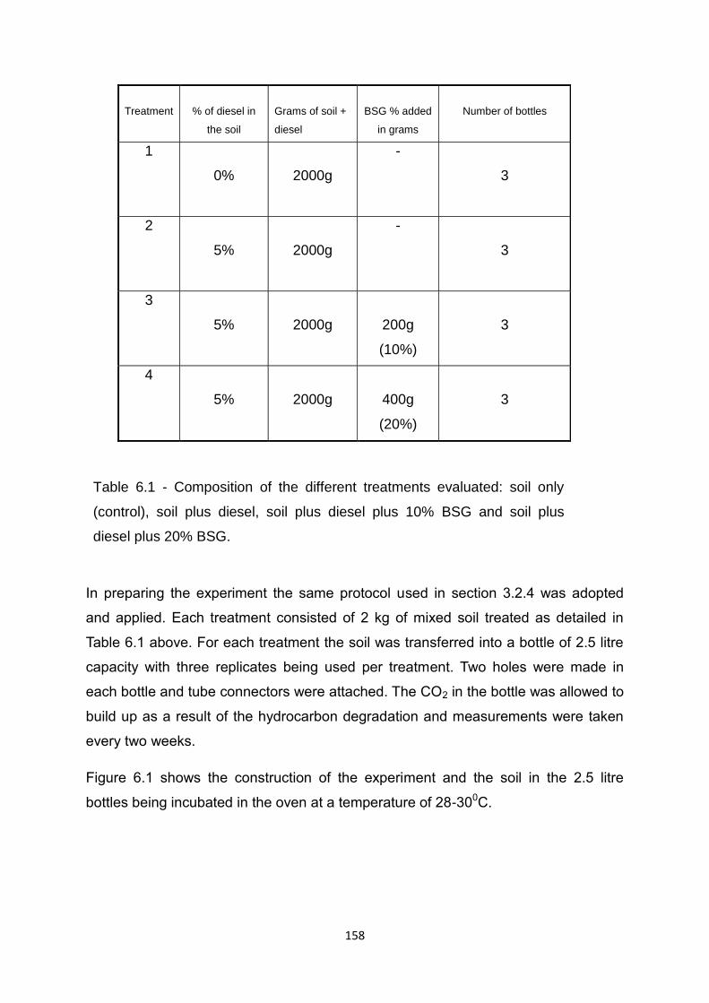
158
Treatment
% of diesel in
the soil
Grams of soil +
diesel
BSG % added
in grams
Number of bottles
1
0%
2000g
-
3
2
5%
2000g
-
3
3
5%
2000g
200g
(10%)
3
4
5%
2000g
400g
(20%)
3
Table 6.1 - Composition of the different treatments evaluated: soil only
(control), soil plus diesel, soil plus diesel plus 10% BSG and soil plus
diesel plus 20% BSG.
In preparing the experiment the same protocol used in section 3.2.4 was adopted
and applied. Each treatment consisted of 2 kg of mixed soil treated as detailed in
Table 6.1 above. For each treatment the soil was transferred into a bottle of 2.5 litre
capacity with three replicates being used per treatment. Two holes were made in
each bottle and tube connectors were attached. The CO2 in the bottle was allowed to
build up as a result of the hydrocarbon degradation and measurements were taken
every two weeks.
Figure 6.1 shows the construction of the experiment and the soil in the 2.5 litre
bottles being incubated in the oven at a temperature of 28-300C.

159
Figure 6.1- The 2.5 litre bottles containing the treatments: soil only, soil plus diesel,
soil plus diesel plus BSG (10%) and soil plus diesel plus BSG (20%)
The following method was adopted to determine the soil respiration at the end of
every two weeks.
6.2.2 Measurement of CO2 and determination of soil respiration
At the end of the two week period CO2 was captured from the bottles using an air
pump. It was collected by bubbling the air plus the CO2 through a solution of sodium
hydroxide. The procedure and method used in collecting the CO2 are broken down
into two sections below:
1. The CO2 trapped in the bottles was captured and transferred into a 250 cms3
Erlenmeyer flask. To do this one of the tubes in the bottle was inserted into an air
pump and the other tube was connected into the top of the 250 cms3 Erlenmeyer
flask, which has a stopper tube connected to it. Then another tube was connected
from the side of Erlenmeyer flask to an arm test tube. The arm test tube has an
opening at the side of it. Figure 6.2 illustrates a conceptual layout of the construction
and how the CO2 was trapped and contained.

160
Figure 6.2: Materials used to trap CO2 from the contaminated soil with diesel in the
laboratory including the air pump to transfer the CO2 into the Erlenmeyer flask and
the test tube used.
The trapped CO2 in the bottle was pumped slowly into the sealed Erlenmeyer flask,
which contains about 50 cms3 (Approximately 1M) of sodium hydroxide. The
pumping process took about 24 hours. The containment of the CO2 in such a closed
compartment and its transfer to a sealed apparatus allows the sodium hydroxide to
absorb the CO2. More so, the purpose of the side arm test tube was to capture
additional CO2 in that if the CO2 in the Erlenmeyer flask does not mix with the
sodium hydroxide the escaping CO2 would be trapped in the side arm test tube.
2. Prior to undertaking the titration the sodium hydroxide from the Erlenmeyer flask
and that from the side arm test tube were mixed in a 250 cm3 Erlenmeyer flask. The
excess sodium hydroxide and sodium carbonate are then titrated as described by
Crossno and Kalbus (1996) as follows:
(a) Each solution was titrated with 1M HCI using phenolphthalein as an indicator.
(b) The volume used was recorded for the first end point.
(c) 4 drops of methyl orange were added and the titration was continued until an

161
orange colour was obtained.
(d) The volume used to the second endpoint was recorded and the amount of CO2
derived from the soil calculated.
The equation used to obtain the mass of CO2 (g) was:
Volume of titrant (L) * molarity of standard acid * molecular weight of CO2
Where
Volume of titrant = 1st to 2nd endpoint
Molarity of standard acid = 1M HCI.
In order to arrive at the actual CO2 (g) the results of the control soil, which was a
treatment without any amendment or without any addition of diesel were deducted
either from the treatment with BSG or treatment without BSG. The average CO2
released from the 100 g of diesel added to the 2 kg of soil during bioremediation
recorded on Day 14, 28, 42, 56, 77, 98 and 129 days are reported in Tables 6.2 to
6.8.
Treatments
types
1 2 3 4 5
Volume of
titrant (L)
molarity
of
standard
acid
molecular
weight of
CO2
Control
soil
result
(g)
Results
(g) CO2
Bioremediation(
10% BSG)
27/1000 1 44.01 0.308 0.88
Bioremediation
20% BSG
30.5/1000 1 44.01 0.308 1.03
Bioremediation
(without BSG)
24.40/1000 1 44.01 0.308 0.77
Control soil 7/1000 1 44.01 0.308 -
Table 6.2: CO2 released after 14 days bioremediation with/without BSG

162
Day 42 CO2 emitted by four types
Treatments
types
1 2 3 4 5
Volume of
titrant (L)
molarity
of
standard
acid
molecular
weight of
CO2
Control
soil
result
(g)
Results
(g) CO2
Bioremediation
10% BSG
10/1000 1 44.01 0.0206 0.23
Bioremediation
20% BSG
12.33/1000 1 44.01 0.0206 0.34
Bioremediation
(without BSG)
9.33/1000 1 44.01 0.0206 0.21
Control soil 7/1000 1 44.01 0.0206 -
Table 6.4: CO2 released after 42 days bioremediation with/without BSG.
Treatments
1 2 3 4 5
Volume of
titrant (L)
molarity
of
standard
acid
molecular
weight of
CO2
Control
soil
result
(g)
Results
(g) CO2
Bioremediation
(10% BSG)
14.88/1000 1 44.01 0.118 0.54
Bioremediation
(20% BSG)
15.77/1000 1 44.01 0.118 0.58
Bioremediation
(without BSG)
8.83/1000 1 44.01 0.118 0.271
Control soil 2.67/1000 1 44.01 0.118 -
Table 6.3: CO2 released after 28 days bioremediation with/without BSG.
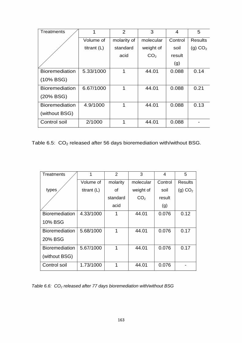
163
Treatments
types
1 2 3 4 5
Volume of
titrant (L)
molarity
of
standard
acid
molecular
weight of
CO2
Control
soil
result
(g)
Results
(g) CO2
Bioremediation
10% BSG
4.33/1000 1 44.01 0.076 0.12
Bioremediation
20% BSG
5.68/1000 1 44.01 0.076 0.17
Bioremediation
(without BSG)
5.67/1000 1 44.01 0.076 0.17
Control soil 1.73/1000 1 44.01 0.076 -
Table 6.6: CO2 released after 77 days bioremediation with/without BSG
Treatments
1 2 3 4 5
Volume of
titrant (L)
molarity of
standard
acid
molecular
weight of
CO2
Control
soil
result
(g)
Results
(g) CO2
Bioremediation
(10% BSG)
5.33/1000 1 44.01 0.088 0.14
Bioremediation
(20% BSG)
6.67/1000 1 44.01 0.088 0.21
Bioremediation
(without BSG)
4.9/1000 1 44.01 0.088 0.13
Control soil 2/1000 1 44.01 0.088 -
Table 6.5: CO2 released after 56 days bioremediation with/without BSG.

164
Treatments
types
1 2 3 4 5
Volume of
titrant (L)
molarity of
standard
acid
molecular
weight of
CO2
Control
soil
result (g)
Results
(g) CO2
Bioremediation
10% BSG
2.67/1000 1 44.01 0.038 0.080
Bioremediation
20% BSG
4.66/1000 1 44.01 0.038 0.17
Bioremediation
(without BSG)
2.67/1000 1 44.01 0.038 0.080
Control soil 0.87/1000 1 44.01 0.038 -
Table 6.7: CO2 released after 98 days bioremediation with/without BSG
Treatments
types
1 2 3 4 5
Volume of
titrant (L)
molarity
of
standard
acid
molecular
weight of
CO2
Control
soil
result
(g)
Results
(g) CO2
Bioremediation(
10% BSG)
4.66/1000 1 44.01 0.015 0.19
Bioremediation
20% BSG
11.55/1000 1 44.01 0.015 0.49
Bioremediation
(without BSG)
3.9/1000 1 44.01 0.015 0.16
Control soil 0.33/1000 1 44.01 0.015 -
Table 6.8: CO2 released after 129 days bioremediation with/without BSG

165
Sample
day
Soil + Diesel
CO2 (g)
Soil + Diesel + 10% BSG
CO2 (g)
Soil + Diesel + 20% BSG
CO2 (g)
Day 14 0.77 0.88 1.01
Day 28 0.27 0.54 0.58
Day 42 0.21 0.23 0.34
Day 56 0.13 0.14 0.21
Day 77 0.17 0.12 0.17
Day 98 0.08 0.08 0.17
Day 129 0.16 0.19 0.49
Total 1.79 2.18 2.97
Table 6.9: CO2 measured on days 14, 28, 42, 56, 77, 98 and 129 for soil plus
diesel, soil plus diesel plus BSG (10%) and soil plus diesel plus BSG (20%).
Table 6.9 provides a summary of the four treatment types of CO2 released when 100
g of diesel was added to (2 kg) of soil during bioremediation activities recorded on
Day 14, 28, 42, 56, 77, 98 and 129 days.
6.3 Data collection
The estimation of the CO2 emitted by bioremediation with and without BSG was
based on the laboratory experiment conducted in this study. The results showed that
using BSG resulted in more CO2 being emitted than in the absence of BSG. The
amount of CO2 obtained from the study was a useful means of ascribing data to the
environmental impacts of bioremediation. In order to assign values for other
remediation techniques information was sourced from a variety of sources such as a
literature search, including professional journals and publications, this information
was then applied to the hypothetical case study site.

166
Actual field data on environmental footprints for the full range of remediation
techniques used for contaminated land sites are sparse, in that it is impractical to
obtain environmental data that would be representative of all project applications,
site types, and conditions. Whilst some case study data are available for sites where
a specific remediation technique has been used the scenario may be difficult to apply
to other remediation methods or sites. Therefore, field data relevant to the
remediation scenario investigated here has been used, when available, to verify
some of the assumptions used in the analysis.
Data has been collected for land, air and water but values will only be assigned to
air, due to the limited availability of data for water and land, environmental emissions
to these media will be qualitatively assessed in relation to the hypothetical site under
study.
Key assumptions and inputs such as energy and emission conversion factors and
average energy used will be considered in the analysis. For example, electricity will
be used as a default factor for all energy consumption for the six different
remediation methods in the study and Heavy Goods Vehicle (HGVs) will be used to
deliver material and waste in the study because of the large volume of soil that was
involved. In addition, it is assumed that the six remediation options under
consideration will achieve more than 90 % of the remediation objective and they will
have the same level of efficiency in terms of removing the diesel contaminants from
the soil.
In this study the values for CH4 and N2O are presented as CO2 equivalent (CO2e)
using a global warming potential factor, consistent with reporting under the Kyoto
Protocol and the second assessment report of the Intergovernmental Panel on
Climate Change (IPCC). The emission of CO2 and other gases such as CH4 and
N2O are potential greenhouse gases (GHGs) and they play major roles in climate
change (IPCC, 2007). Each gas has a global warming potential measured as the
ratio of heat trapped by one metric tonne of gas to that of one tonne of CO2 over a
specific time period (TRUCOST, 2012) usually 100 years (Colpan et al., 2009). The
emissions of these GHGs multiplied by their Global Warming Potential (GWP) are
used to calculate the equivalent level of CO2e emissions (Colpan et al. 2009).
The conversion factors allow activities data such as litres of fuel used, number of

167
miles driven, tonnes of waste sent to landfill to be converted into kilograms of CO2
equivalent (Defra/DECCs, 2011). Therefore, CO2e is a term to describe the different
greenhouse gases in a common unit (Brander and Davis, 2012). The analysis used
in the study is structured so that data that is universally accepted can be used and
incorporated subject to adjustment in the units of measurement. The following
section shows the spread sheet including the inputs and assumption data used in the
analysis.
6.3.1 Emission factors and their Justification

168
The factors presented in table 6.10 were derived from the conversion factors
presented in (Defra/DECC, 2011). These emission factors are based on g per vehicle
km travel. They are used to calculate the g of pollutant concentration in the air. In the
U.K. emissions for key air pollutants such as NOx, PM10, PM2.5, NMVOC, and CO
are calculated by using speed related activity and vehicle flows on the road network.
The exceptions are CO2, CH4 and N2O which uses fuel consumption as a proxy for
the distribution of emissions. Emission estimates in the UK are calculated by
applying an emission factor to an appropriate activity as indicated below:
Emission = Factor x Activity
The emission factors are based on experimental measurements of emissions from
in-service vehicles of different types driven under a test cycle with different average
speeds (NAEI, 2006). Thus, pollutant concentrations in the air can be measured
through a vehicle driven cycle by using road traffic data, vehicle kilometres travelled
for different vehicle types and different road classifications on the U.K road network.
Emission factors are normally obtained from measurements on a number of sources
representatives of a particular sector (NAEI, 2008). For example emission factors for
vehicles pollutants are compiled by National Atmospheric Emission Inventory (NAEI)
using fuel consumption and emissions factors derived from the database held by the
Transport Research Laboratory (TRL) measured over different test cycles (NAEI,
2008). While activities data are derived from Government statistical sources such as
U.K. Energy statistics, Transport Statistics Great Britain and others such as U.K.
Petroleum Industries Association (UKPIA), which provide data on the sulphur content
of fuels (NAEI, 2008).
In the study here all greenhouse gas emissions have been converted into carbon
dioxide equivalent (CO2e) and it will be reflected in metric tonnes which are used in
reporting emissions under the Kyoto protocol. The CO2e for CO2, CH4 and N2O for
Heavy Goods vehicles such as tractors have already had CO2e incorporated in the
emissions factors presented in Table 6.10 and as such need not be calculated
separately. However, in the assessment of a particular remediation activity where
CO2e has not been reported, the conversion factors and their global warming
potential will need to be applied using the values in Table 6.10.1.

169
No. Data Values Sources/references
1 CO2 to CO2e 1 DEFRA/DECC, 2011 GHG conversion factor 2 CH4 to CO2e 21
3 N2O to CO2e 310
4 CO2 from electricity per kWh (1.37 ibs) equivalent in kg
0.6214 U.S. EIA, 2005 and Electricity power annual, 2005
Electricity consumed by SVE component over 3 years
5 Electricity consumption for Vacuum blower measured kWh
108,000 U.S. EPA, 2010
6 Electricity consumption for Off-gas treatment facility measured kWh
90,000
7 Electricity consumption for data monitoring and processing measured kWh
33,000
8 Electricity consumption for above ground treatment structure measured kWh
1,800
Total electricity consumed kWh
232,800
Electricity consumed by thermal desorption with a year
9 M3
of soil will generate electricity measured kWh
342 Baker, 2011 11 10,000 m
3 of soil will generate
electricity measures kWh 3,420,000
Fuel usage
12 For 9.7 miles amount of litres of fuel used for HGVs in U.K
4.54609 Department for transport and statistics, 2010
13 14 excavating tractor uses litres of diesel
70 Sirius, 2010
14 Litres of fuel used for bioremediation with BSG
910 Appendix lll
15 Litres of fuel used for bioremediation without BSG
1330 Appendix lll
Distance of site location
16 Estimated distance of the site in Sunderland To Hartlepool measured in km
48.28 Pers.comm, 2012- meeting
170
These values were used for calculating the CO2e for bioremediation with and without
BSG, natural attenuation, landfill disposal, SVE and thermal desorption. The values
use for the calculation of the various emissions is presented in Table 6.10.1 above.
The values for CO2e used in the study were derived from conversion factors
presented by Defra/DECC (2011). These are key pollutants that affect climate
change or lead global warming. Other CO2 calculations were from the use of
electricity and in the U.S. it was measured as 1.37 ibs/kWh, which is equivalent of
0.6214 kg/ kWh. In the study reported here the same value was used to calculate
electricity usage for SVE and thermal desorption. The electricity consumption was
based on components (machines) used in treating the volatile organic compounds or
the vapour gases. For SVE it was calculated for 3 years and for thermal desorption it
was based on m3 of soil per kWh (U.S. EPA, 2010a and Baker et al. 2011).
In the study reported here heavy goods vehicles (HGVs) were used in tipping,
transporting wastes and materials from the contaminated site to the disposable
location, they were also used in excavating and turning of the soil during the
bioremediation process. To derive the emission for a particular pollutant the emission
conversion factor is applied to the distance covered for that journey (NAEI, 2008).
The NAEI is the main repository of U.K. data on all types of atmospheric emission
from all sources (NAEI, 2012) and the activity data are obtained from the Department
of Transport (DFT). In order to derive the activities that lead to the emissions used in
the study the distance covered from Sunderland to Hartlepool was estimated to be
48.28 km (Pers.comm, 2011) and 4.54609 litres of fuel are expected to be used to
cover 9.7 miles (Dft, 2010). The heavy machinery used in excavating and turning the
soil is expected to consume 70 litres of fuel daily this value was used to derive the
amount of fuel used for bioremediation with and without BSG (Appendix 111).
As part of the commitments to the Convention on Long-Range Trans boundary Air
Pollution (CLRTAP), countries are mandated to submit emission projections for NOx,
SOx, NMVOC and NH3 under the Gothenburg Protocol (NAEI, 2012). These
pollutants are also covered under the Directive 201/81/EC of the European
Parliament and the Council on National Emissions Ceilings (NECD) and some of
these emissions are covered under the UN Framework Convention on Climate
Change (UNFCCC) including carbon dioxide, nitrous oxide, methane,
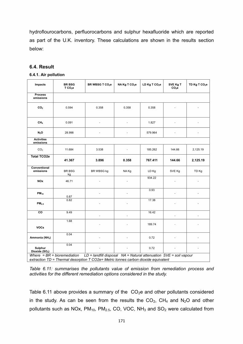
171
hydroflourocarbons, perfluorocarbons and sulphur hexafluoride which are reported
as part of the U.K. inventory. These calculations are shown in the results section
below:
6.4. Result
6.4.1. Air pollution
Impacts
BR BSG T CO2e
BR WBSG T CO2e
NA Kg T CO2e
LD Kg T CO2e
SVE Kg T
CO2e
TD Kg T CO2e
Process emissions
CO2
0.594
0.358
0.358
0.358
-
-
CH4
0.091
-
-
1.827
-
-
N2O
28.998
-
-
579.964
-
-
Activities emissions
CO2
11.684
3.538
-
185.262
144.66
2,125.19
Total TCO2e 41.367
3.896
0.358
767.411
144.66
2,125.19
Conventional emissions
BR BSG
kg
BR WBSG kg
NA Kg
LD Kg
SVE Kg
TD Kg
NOx
46.71
-
-
934.22
-
-
PM10
0.87
-
-
0.93 -
-
PM2.5
0.82 -
-
17.38 -
-
CO 9.49 -
-
16.42 -
-
VOCs
1.68 -
-
189.74
-
-
Ammonia (NH3)
0.04 -
-
0.72
-
-
Sulphur
Dioxide (SO2)
0.04 -
-
0.72
-
-
Where = BR = bioremediation LD = landfill disposal NA = Natural attenuation SVE = soil vapour extraction TD = Thermal desorption T CO2e= Metric tonnes carbon dioxide equivalent
Table 6.11: summarises the pollutants value of emission from remediation process and activities for the different remediation options considered in the study.
Table 6.11 above provides a summary of the CO2e and other pollutants considered
in the study. As can be seen from the results the CO2, CH4 and N2O and other
pollutants such as NOx, PM10, PM2.5, CO, VOC, NH3 and SO2 were calculated from

172
remediation processes and activities such as transportation and energy. The detailed
calculations of each remediation technique are described in the next section.
6.4.2 Bioremediation emissions
The total volume of CO2 evolved from the bioremediation process with BSG was
previously calculated to be 2.97 g and without BSG was 1.79 g when the soil volume
was 2 kg with 5% diesel contaminants (100 g) in Table 6.9. These values were
obtained from the respirometry experiment carried out in the laboratory in section
6.2.2. While in the hypothetical site used in the study the mass of contaminants was
20,000 kg (diesel) in the 10,000 m3 of soil. In order to arrive at the amount of C02 in
the study here the initial value of CO2 obtained in the laboratory was extrapolated.
Therefore, if the treatment with soil plus diesel plus 20% BSG generated 2.97 g of
CO2 when 100 g of diesel was added then CO2 that would be generated if 20,000 kg
(20,000,000 g) of contaminants were remediated can be calculated to be 594 kg
(2.97 * 20,000,000 /100). In order to calculate the CO2e the value of 594 are
converted into metric tonnes and the resultant value is multiplied by 1 which is the
standard of Global warming potential (table 6.10). The calculation is as follows:
1 metric tonnes = 1000 kg
594 kg CO2 = 0.594 metric tonnes CO2
0.594 metric tonnes CO2 * 1 = 0.594 metric tonnes CO2e.
However, in rationalising the values of CO2 in the study with treatment with BSG and
treatment without BSG it was evident in the laboratory study that the addition of BSG
emitted more CO2 than when the soil has no nutrient amendment (Table 6.9). This
will lead to a different time frame for the remediation target to be met. Since the goal
of the research is to achieve the same remediation target of more than 90% of the
diesel to be removed from the soil the bioremediation processes without the addition
of BSG would achieve the remediation objective but later than the treatment with
BSG (results of Chapter 4). But the C02 that would be emitted will be slower as
indicated in the respirometry results and this value is 1.79 g for 129 days.
The value of CO2 from bioremediation without BSG if 20,000 kg (20,000,000 g) of
contaminants were remediated can be calculated to be 358 kg (1.79 * 20,000,000
173
/100). In order to calculate the CO2e the value of 358 kg are converted into metric
tonnes and the resultant value is multiplied by 1 which is the standard of global
warming potential (table 6.10). The calculation is as follows:
1 metric tonnes = 1000 kg
358 kg CO2 = 0.358 metric tonnes CO2
0.358 metric tonnes CO2 * 1 = 0.358 metric tonnes CO2e.
Other emissions resulting from bioremediation include activities that result in CO2,
CH4 and N2O arising from the transportation of BSG from Hartlepool to Sunderland
and turning of the soil during bioremediation. Table 6.12 and 6.13 below shows the
calculation of CO2 CH4 and N2O resulting from transporting BSG from Hartlepool to
Sunderland.

174
Thus, the distance from Sunderland to Hartlepool has been determined to be 30
miles or 48.28 km (table 6.10). Since there was 2000 tonnes of BSG to be delivered
using 16 tonne load lorries. It was estimated that it would take 125 trips to deliver the
2000 tonnes BSG. The total distance covered given the 125 trips would be 12,070
km.
Pollutants
Factors gCOe per
vehicle KM
Kilometre travel
Emissions gCOe
CO2 at 0% load
671.5
6,035
4,052,502.5
CO2 at 100% load
863.4
6,035
5,210,619
Total 12,070 9,263121.5
Table 6.12: Loading vehicle factors for 0% and 100% which were applied
to the kilometre travel to derive the emissions gCO2 for BSG as a result of
the vehicle movement from Hartlepool to Sunderland.
Pollutants
Factors gCOe per
vehicle KM
Kilometre travel
Emissions gCOe
CH4 at 0% and 100%
load
0.36
12,070
4,345.2
N2O at 0% and 100%
load
7.75
12,070
93,542.5
Table 6.13: Loading vehicle factors for CH4 and N2O at 0% and 100%
which were applied to the kilometre travel to derive the emissions gCO2 for
BSG as a result of the vehicle movement from Hartlepool to Sunderland.

175
However, there are different emission factors for running a vehicle empty and for full
loads; as such 671.5 g was the emission factor for running a vehicle empty and
863.4g for running a full loaded vehicle (Table 6.10). Applying the different emission
factors of running a vehicle empty and full load would amount to 4,052,502.50 gCO2e
and 5,210,619 gCO2e for empty and full loading respectively. Therefore, the total CO2
to transport the BSG from Hartlepool to Sunderland would be 9,263,121.50 gCO2e
(9,263.12 kgCO2e). Similarly, the values of emissions for CH4 and N2O are calculated
by multiplying their respective emission factors to the total distance covered to
deliver the BSG from Hartlepool to Sunderland. From Table 6.13 the value for CH4 is
4,345.20 g (4.345 kg) and N2O 93,542.50 g (93.543 kg). As CO2e are usually
measured in metric tonnes the derived value is divided by 1000 and the resultant
value is multiplied by 21 and 310 for CH4 and N2O respectively, which are the
standard of global warming potential (table 6.10The calculation is as follows:
For CH4
1 metric tonnes = 1000 kg
4.345 kg CO2 = 0.004345 metric tonnes CO2
0.004345 metric tonnes * 21 = 0.091 tonnes CO2e
For N2O
1 metric tonnes = 1000 kg
93.543 kg CO2e = 0.093543 metric tonnes CO2e
0.093543 metric tonnes * 310 = 28.998 tonnes CO2e
In addition, CO2 emissions with bioremediation were also associated with the use of
14 tonne excavator machinery, which has been estimated to consume diesel fuel of
910 litres for bioremediation with BSG and 1,330 litres for bioremediation without
BSG.

176
Applying the emission factor for a heavy tractor of 2.66 kg (table 6.10) to the amount
of red diesel consumed by the tractor during turning and tilling would amount to
2,420.60 kgCO2 and 3,537.80 kgCO2e for bioremediation with BSG and
bioremediation without BSG respectively. To derive the total CO2e from
bioremediation with BSG would be the summation of the CO2 from combustion of
fossil fuel by freight transportation of the BSG and CO2 from turning the soil during
bioremediation, which amounts to 11,683.72 kg CO2e (2,420.60 kg + 9,263.12 kg).
As CO2e are usually measured in metric tonnes the derived value are divided by
1000. The calculation is as follows:
For bioremediation
1 metric tonnes = 1000 kg
11,683.72 kg CO2e = 11.684 metric tonnes CO2e
For bioremediation without BSG
1 metric tonnes = 1000 kg
3,537.80 kg CO2 = 3.5378 metric tonnes CO2e.
Pollutants
Factors
kgCO2e
Amount diesel
used/litres
Emissions
kgCO2e
Kg/CO2e/Litre (bioremediation
with BSG)
2.66
910
2,420.60
KgCO2e/Litre (bioremediation
without BSG)
2.66
1330
3,537.80
Table 6.14: Calculation of CO2e derived by multiplying emission factors by
the amount of diesel consumed for bioremediation with BSG and
bioremediation without BSG as a result of the use of excavator machine.

177
Emissions from NOx, PM10, PM2.5, CO, VOC, NH3, and SOx which are recorded in g
per km, emissions values in table 6.15 are derived by multiplying their activities data
which is the distance covered for transporting BSG with their respective emission
factors. The total distance travelled has been determined to be 12,070 km given the
125 trips and the emission factors can be found in Table 6.10. The value for NOx
was calculated to be 46,710.9 g, PM10 869.04 g for PM2.5 estimated to be 820.76 g
CO 9,487.02 g, VOC 1,677.73 g, NH3 36.21 g, and SOx 36.21 g.
6.4.3. Natural attenuation processes (CO2)
Few studies have evaluated the mass of CO2 released during natural attenuation.
However, over the estimated five year period for breakdown to occur it is likely that
all of the hydrocarbon present will be broke down and released as CO2.
However, the laboratory study using BSG showed that CO2 generated when 20%
BSG was added to the soil was 2.97 g at the end of 129 days and CO2 generated
without the addition of BSG was 1.79 g (table 6.9) at day 129. Natural attenuation
Pollutants Factors
g/ km
Vehicle Kilometre
travel
Total
Emissions g
Nitrox oxide (NOx) 3.870 12,070 46,710.9
Particulate Matter
(PM10)
0.072 12,070 869.04
Particulate Matter
(PM2.5)
0.068 12,070 820.76
Carbon Monoxide
(CO)
0.786 12,070 9,487.02
Volatile organic
compound (VOC)
0.139 12,070 1,677.73
Ammonia (NH3) 0.003 12,070 36.21
Sulphur Dioxide (SO2) 0.003 12,070 36.21
Table 6.15: showing calculation of NOx, PM10, PM2.5, CO, VOC, CO, NH3
and SO2 emitted by vehicle movements through the delivery of brewery
spent grain from Hartlepool to Sunderland.

178
occurs without human intervention and CO2 release will be slower than when the
condition of the soil is modified such as with the addition of BSG. It was evident in
the laboratory study that the addition of BSG emitted more CO2 than when the soil
has no nutrient amendment. Therefore, CO2 from natural attenuation will be equated
to that found in the laboratory study when no BSG was added because given the five
years duration the same amount of CO2 would be emitted but in a slower manner
and the amount generated was expected to be equivalent to 1.79 g over a 5 year
period.
In addition, the 5 year baseline adopted to achieve natural attenuation in the study
could be regarded as a good situation for defining and assessing the baseline
scenario because the data was obtained from a remediation company performance
report, project manager and vendor (Sirius, 2010). Since the contaminant
concentration was 20,000 kg the CO2 that would evolve from the natural attenuation
is expected to be equivalent to the amount generated when bioremediation without
BSG was an alternative. This is because the process follows a similar pattern, as
microbial activities result in the degradation of the organic compounds.
The results of the respirometry study have determined the value of CO2 without the
addition of BSG to be 1.79 g and the expected remediation objective was to be
achieved in 9 months. Also, the same amount of CO2 would be emitted if natural
attenuation was adopted and the remediation objective was expected to be achieved
in 5 years given the 20,000 kg of contaminants the total CO2 would be 358 kg (1.79 *
20,000,000/100). In order to calculate the CO2e the value of 358 kg are converted
into metric tonnes and the resultant value is multiplied by 1 which is the standard of
global warming potential (table 6.10). The calculation is as follows:
1 metric tonnes = 1000 kg
358 kg CO2 = 0.358 metric tonnes CO2
0.358 metric tonnes CO2 * 1 = 0.358 metric tonnes CO2e.
6.4.4. Landfill disposal option (CO2)
Landfills have the potential for a range of negative impacts on the environment and
human health, including a major cause of pollution to groundwater and surface water

179
across Europe (Defra, 2005). The presence of wastes in landfills will result in the
decay of the organic matter and generation of CH4 and CO2. Landfills have been
identified as significant anthropogenic sources of atmospheric CH4 and are believed
to account for 6-18% of the total CH4 emissions in the world (Houde et al. 1997).
When oxygen is used up bacteria begin to produce CH4. The more oxygen is present
in a landfill, the longer aerobic bacteria can decompose waste (URL8). But if the
waste is highly compacted (without oxygen), CH4 production will begin earlier as the
aerobic bacteria are replaced by methane-producing anaerobic bacteria (URL8) and
CH4 is generated in the landfill as the waste decomposes.
CH4 lifetime in the atmosphere is much shorter than CO2 but CH4 is more efficient at
trapping radiation than CO2 (EPA, 2010b). The comparative impact of CH4 on climate
change is over 20 times that of CO2 over a 100 year period (EPA, 2010b). However,
CH4 produced at landfills need not be released to the atmosphere but can be used
as landfill gas. CH4 and CO2 landfill gas can be recovered and used directly in local
electrical generators or as a feedstock for producing natural gas (EPA, 2010b). But in
the calculation reported here breakdown of wastes in landfill will only be assessed as
CO2 production. However, wastes deposited in landfill are usually converted to both
CO2 and CH4 and will eventually be expected to disperse to the environment as CO2
and CH4.
The emission of CO2 from landfill in the study reported here would be calculated
from the degradation of the organic compound. It was assumed in the study that
20,000 kg of contaminant was deposited in the landfill. The 20,000 kg of contaminant
would be used as a proxy to evaluate the amount of CO2 that would be evolved
when the contaminated soil was landfilled. Although CO2 from biodegradable waste
does not pose a risk to the environment however if it emanates from hydrocarbons it
would contribute to global warming and should be estimated when reporting
emissions (IPCC, 2006).
Therefore, the 20,000 kg of contaminants depicted in the conceptual site model
would be assumed to have been dispersed to the environment when landfill disposal
was a possible option. Because depositing the contaminated soil to landfill will
require a longer time for the waste to be degraded in the landfill the value of CO2
adopted for natural attenuation and bioremediation without BSG will be used as the

180
same amount of contaminants that would have been emitted. This value is
necessary because soil contaminated with diesel fuel is regarded as biodegradable
waste and falls under the classification of hazardous waste (Defra, 2005) and in
landfill deposited wastes are allowed to degrade over time and are converted to CO2
and CH4.
In the study here the value of CO2e during bioremediation without BSG was
previously estimated to be 358 kg. In order to calculate the CO2e the value of 358 kg
are converted into metric tonnes and the resultant value is multiplied by 1 which is
the standard of global warming potential (table 6.10). The calculation is as follows:
1 metric tonnes = 1000 kg
358 kg CO2 = 0.358 metric tonnes CO2
0.358 metric tonnes CO2 * 1 = 0.358 metric tonnes CO2e.
There are also other CO2 emissions associated with landfill disposal as a result of
the movement of vehicles for the disposal and re-fill of the contaminated soil. The
emissions are calculated by multiplying the distance travelled by the vehicle and the
emission factors related to the journey. Table 6.16 and 6.17 show the calculations of
CO2 for disposing and re-filling the earth from Sunderland to Hartlepool.

181
Pollutants
Factors gCO2e per
vehicle KM
Kilometre travel
Emissions
gCO2e
CO2 at 0% load
671.5
60,350
40,525,025
CO2 at 100%
load
863.4
60,350
52,106,190
Total
120,700
92,631,215
Table 6.16: Calculation of gCO2e emissions derived by multiplying emission
loading factors of CO2 to kilometres travelled during vehicle movement including
empty and full load for disposal of the soil from Sunderland to Hartlepool.
Pollutants
Factors gCOe per vehicle
KM
Kilometre travel
Emissions gCOe
CO2 at 0%
load
671.5
60,350
40,525,025
CO2 at
100% load
863.4
60,350
52,106,190
Total 120,700 92,631,215
Table 6.17: Calculation of gCO2e emissions derived by multiplying emission
loading factors of CO2 to kilometre travel during vehicle movement including
empty and full load for re-filling the site with new topsoil from Hartlepool to
Sunderland
The conversion factor for running empty Heavy Goods Vehicles (HGVs) and a full
load were previously calculated as 671.5 and 863.4 respectively (table 6.10). It has
previously been estimated in chapter 5 that it would take 384 tonnes of soil to be

182
disposed of daily using 16 lorry loads. The 20,000 tonnes of soil would require 1,250
trips to cover the entire journey and the distance from Sunderland to Hartlepool was
previously estimated to be 48.28 km. In order to complete a journey the lorry is
expected to run a full load and an empty load to dispose of the soil. Therefore, it will
require 120,700 km to dispose of the 20,000 tonnes taking into consideration running
the vehicle empty and full (48.28 X2 = 96.56 X 1250).
Since CO2 are calculated based on the consumption of fuel used and the total
distance covered for the entire journey. Table 6.16 and 6.17 shows the total distance
travelled and the emission factors taking into consideration the consumption of fuel
used when the vehicle is run empty and full and applying the related emission factors
would amount to CO2 of 185,262,430 g for disposing of the soil and for re-filling the
site. In order to calculate the CO2e the value of both disposing and re-filling are
added together (92,631,215 g * 2 = 185,262,430 g) and converted into metric tonnes
and multiplied by 1 which the global warming potential. The calculation is as follows:
1 metric tonnes = 1000 kg
185,262.43 kg CO2e = 185.262 metric tonnes
185.262 metric tonnes * 1 = 185.262 metric tonnes CO2e

183
In addition, there were other emissions of CH4 and N2O that are calculated from the
total kilometres travelled for disposing of and re-filling the soil. Table 6.18 and 6.19
shows the total values of CH4 and N2O calculated in gCO2e per km. The total
distance covered for disposing of the soil has previously been estimated to be
120,700 km including empty and full loads and the emissions factors of CH4 and N2O
are the same values (table 6.10).
Applying the related emission factors would amount to 86,904g and 1,870850g for
disposing and for re-filling the site for CH4 and N2O respectively. These include the
net values from Table 6.18 and 6.19 for CH4 (43,452 +43,452 = 86,904 g) and N2O
(935,425 + 935,425 = 1,870,850 g). As CO2e are usually measured in metric tonnes
Pollutants Factors gCO2e per
vehicle KM
Kilometre travel Emissions gCO2e
CH4 at 0% and
100% load
0.36 120,700 43,452
N2O at 0% and
100% load
7.75 120,700 935,425
Table 6.18: Calculations of CH4 and N2O emissions by multiplying
kilometre travel by emission loading factors including full and empty
loading during disposing of the soil to landfill from Sunderland to
Hartlepool.
Pollutants Factors gCO2e per
vehicle KM
Kilometre travel Emissions gCO2e
CH4 at 0% and
100% load
0.36 120,700 43,452
N2O at 0% and
100% load
7.75 120,700 935,425
Table 6.19: Calculations of CH4 and N2O emissions by multiplying
kilometre travel by emission loading factors including full and empty
loading during re-filling of the soil from Hartlepool to Sunderland.
184
the derived value is divided by 1000 and the resultant value is multiplied by 21 and
310 for CH4 and N2O respectively, which are the standard of global warming
potential (table 6.10).
The calculation is as follows:
For CH4
1 metric tonnes = 1000 kg
86.904 kg CO2e = 0.087 metric tonnes
0.087 metric tonnes * 21 = 1.827metric tonnes CO2e
For N2O
1 metric tonnes = 1000 kg
1,870.85 kg CO2e = 1.871 metric tonnes CO2e
1.871 metric tonnes * 310 = 579.964 metric tonnes CO2e.
Other conventional emissions associated with vehicles movement were NOx, PM10,
PM2.5, CO, VOC, NH3 and SO2. Vehicle movements for disposing of soil to landfill
and re-fill of the site were already estimated to be 241,400 km which was a
combination of a distance of 120,700 km for disposal of the soil and 120,700 km for
re-filling of the site (table 6.18 and 6.19.).

185
Applying the various emissions factors to the distance travelled would result in the
total emissions for a particular pollutant. Table 6.20 showed the total emissions for
the different pollutants calculated in g per km for NOx is 934,218 g, for PM10 would
be 17,380.8 g, PM2.5 16,415.20 g, CO 189,740.40 g, VOC 33,554.60 g, NH3 724.20 g
and SO2 724.20 g.
6.4.5. Soil vapour extraction (CO2)
SVE involves the contaminants being captured by a ventilation system, pre-heated,
and thoroughly mixed and combusted at a high temperature. The contaminants are
converted to innocuous end products in the form of CO2 and water. Sufficient heating
of a volatile organic compound in the presence of oxygen will convert the VOCs to a
harmless end product (AICE, 1993 and U.S EPA, 2006.).
Using SVE treatment facility such as thermal treatment technologies could destroy
hydrocarbons in a vapour stream at an elevated temperature by oxidizing the
hydrocarbons to CO2 and water (U.S EPA, 2006). Catalytic oxidation is regarded as
the most common thermal treatment off-gas technology; the system uses a catalyst
together with heat to oxidize contaminants in a vapour stream (U.S. EPA, 2004). The
Pollutants Factors
g/km
Vehicle Kilometre travel Emissions g
Nitrox oxide (NOx) 3.870 241,400 934,218
Particulate Matter
(PM10)
0.072 241,400 17,380.8
Particulate Matter
(PM2.5)
0.068 241,400 16,415.20
Carbon Monoxide (CO) 0.786 241,400 189,740.40
Volatile organic
compound (VOC)
0.139 241,400 33,554.60
Ammonia (NH3) 0.003 241,400 724.20
Sulphur Dioxide (SO2) 0.003 241,400 724.20
Table 6.20: Calculation of NOx, PM10, PM2.5, CO, VOC, CO, NH3 and SO2
emitted by vehicle movement through disposing and re-filling of the soil
from Hartlepool to Sunderland and values are derived by multiplying the
kilometre travel by various emission factors.
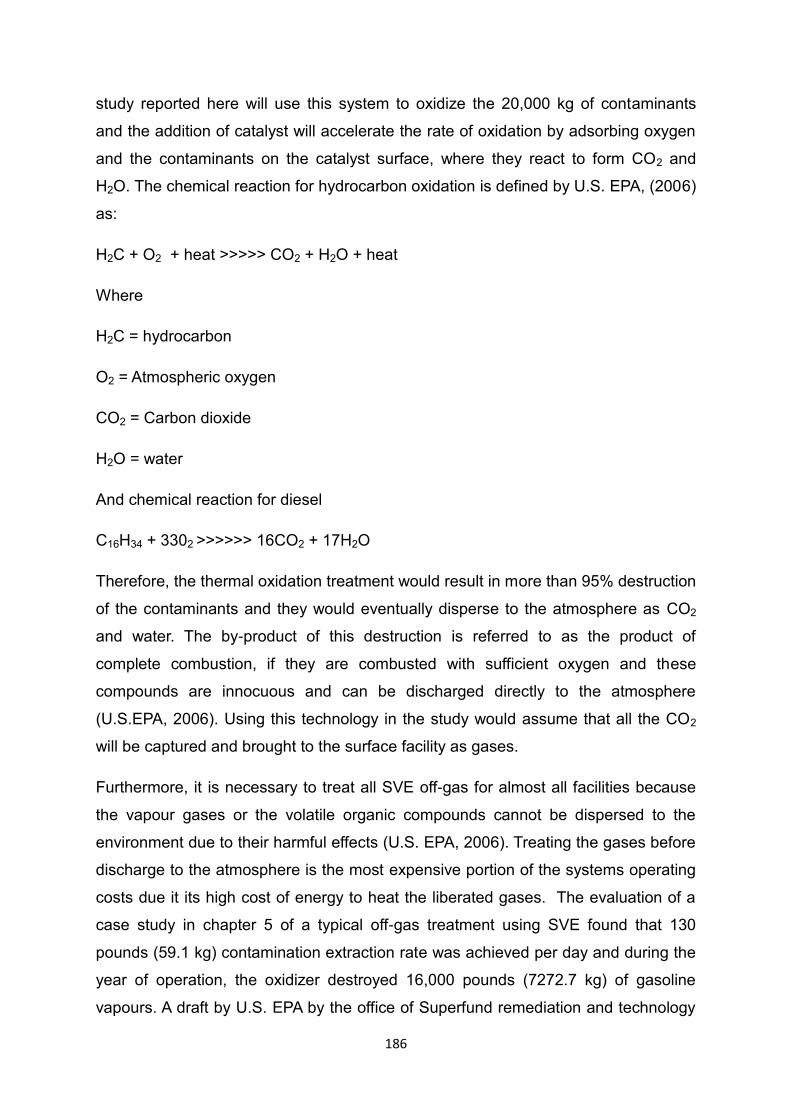
186
study reported here will use this system to oxidize the 20,000 kg of contaminants
and the addition of catalyst will accelerate the rate of oxidation by adsorbing oxygen
and the contaminants on the catalyst surface, where they react to form CO2 and
H2O. The chemical reaction for hydrocarbon oxidation is defined by U.S. EPA, (2006)
as:
H2C + O2 + heat >>>>> CO2 + H2O + heat
Where
H2C = hydrocarbon
O2 = Atmospheric oxygen
CO2 = Carbon dioxide
H2O = water
And chemical reaction for diesel
C16H34 + 3302 >>>>>> 16CO2 + 17H2O
Therefore, the thermal oxidation treatment would result in more than 95% destruction
of the contaminants and they would eventually disperse to the atmosphere as CO2
and water. The by-product of this destruction is referred to as the product of
complete combustion, if they are combusted with sufficient oxygen and these
compounds are innocuous and can be discharged directly to the atmosphere
(U.S.EPA, 2006). Using this technology in the study would assume that all the CO2
will be captured and brought to the surface facility as gases.
Furthermore, it is necessary to treat all SVE off-gas for almost all facilities because
the vapour gases or the volatile organic compounds cannot be dispersed to the
environment due to their harmful effects (U.S. EPA, 2006). Treating the gases before
discharge to the atmosphere is the most expensive portion of the systems operating
costs due it its high cost of energy to heat the liberated gases. The evaluation of a
case study in chapter 5 of a typical off-gas treatment using SVE found that 130
pounds (59.1 kg) contamination extraction rate was achieved per day and during the
year of operation, the oxidizer destroyed 16,000 pounds (7272.7 kg) of gasoline
vapours. A draft by U.S. EPA by the office of Superfund remediation and technology
187
innovation estimated electricity consumption and CO2 emission for typical SVE
system in U.S. In the analysis the annual estimated electricity use for 3 years was
232,148 kWh (U.S. EPA, 2008a) and this estimate has been used to project CO2 by
the U.S. EPA from 2008 to 2030.
However, a similar evaluation carried out in 2010 using best management practices
(BMPs) and the sampling of electricity consumed by SVE components for three
years excluding system design and construction was estimated to be 232,800 kWh
(U.S. EPA, 2010a). This could emit 184 tons of CO2 based on the average U.S fuel
mix, which is equivalent to the electricity used by nearly 22 homes a year (U.S. EPA,
2010a).
In the study here using the same SVE components (table 6.10) such as thermal
oxidation where the treatment facility will oxidize the diesel pollutants and convert it
into CO2 and water. The harmless products would be discharged to the atmosphere
and it would be monitored by the use of a continuous detection systems (FID) used
by AAA construction (URL7) where any incomplete combustion will be checked and
treated accordingly and in compliance with the limit of the laws.
Since 20,000 kg of contaminants will be destroyed in a 3 year period for the
remediation objective to be met, it would require the same amount of energy of
232,800 kWh specified above to destroy all the contaminants. But the use of this
facility will generate CO2, due to electricity consumption and CO2 emitted/kWh
generated is 1.37 Ibs or 0.6214 kg (table 6.10). Convertibly the SVE treatment during
the 3 years of operation will generate a total CO2 of 144,661.92 kg (232,800 *
0.6214). In order to calculate the CO2e the value of 144,661.92 kg are converted
into metric tonnes and the resultant value is multiplied by 1 which is the standard of
global warming potential (table 6.10). The calculation is as follows:
1 metric tonnes = 1000 kg
144,661.92 kg CO2 = 144.662 metric tonnes CO2
144.662 metric tonnes CO2 * 1 = 144.662 T CO2e.
6.4.6. Thermal desorption
In the in-situ thermal desorption facility, vaporization is the main mechanism used to

188
enhance recoveries of volatile organic compounds. The in situ thermal desorption
method had been designed and implemented and consistently produced more than
95% mass removal in clay soil (Baker et al. 2008). The technique in the present
study involves the simultaneous application of heat by thermal conduction and SVE
to remove the diesel from the soil. The processes involve using recovery wells to
capture both liquids and gases and transport them to the subsurface facility for
treatment. Thus, various residuals are usually generated from the thermal process.
Some of these are hazardous others are non-hazardous, but diesel fuels are
certainly hazardous and would be condensed to a liquid form or treated as off-gas.
In the case study reviewed in chapter 5 the energy consumption during in situ
thermal desorption when 11,100 m3 of soil volume for 6 months was treated was 342
kWh/m3. This corresponds to 3,796,200 kWh of electricity use for 11,100 m3 when all
the components that used electricity were included. According to the review
conducted by the U.S. EPA, (2008b) where all the components that use electricity or
energy were reviewed and analysed at Superfund clean-up sites using five
remediation technologies including thermal desorption to treat contaminated material
such as hydrocarbon, it was found that electricity usage accounts for 89% of total
energy cost. The amount of electricity use accounted for 95% of total CO2 emissions
and fuel accounted for 5%.
In the study here if the same technology that was used to remediate the 11,100 m3 in
the Reerslev site in Denmark, was used, the remediation target could be achieved in
6 months. Converted to the actual soil volume of 10,000 m3 in the study here in
order to achieve up to 95% clean-up level for 6 months using the same in situ
thermal desorption facility, would require predicted energy of 3,420,000 kWh of (342
kWh/ m3 * 10,000 ). The contaminant would be captured and destroyed in an
afterburner which is a surface facility to treat off-gas materials. The amount of
contaminants to be treated was previously estimated to be 20,000 kg of organic
compounds. But CO2 emitted per kWh of electricity was estimated to be 1.37 Ibs
(0.6214 kg) as indicated in table 6.10. Then the thermal desorption facility in the
study is expected to operate for six months and will generate a total CO2 of
2,125,188 kg (3,420,000 x 0.6214 kg). In order to calculate the CO2e the value of
2,125,188 kg are converted into metric tonnes and the resultant value is multiplied
by 1 which is the standard of global warming potential (table 6.10). The calculation

189
is as follows:
1 metric tonnes = 1000 kg
2,125,188 kg CO2 = 2,125.19 metric tonnes CO2
2,125.19 metric tonnes CO2 * 1 = 2,125.19 T CO2e.
6.5. Impacts of remediation activities on water and land
Pollution incidents are most likely to lead to water or land damage where the incident
results in serious contamination of soil on the surrounding land. In addition, the
mitigation action put in place should not contribute additional damage to the land or
surrounding water. The majority of times environmental damage may be in the form
of new pollution, as a result of chemical use, during the period of remediation or from
transferring the contaminants to a different location where it may affect surface water
or underground water. In the study here the hydrocarbon contamination does not
affect underground water or surface water as shown in the hypothetical site.
However, the adoption of any remediation method could result in contamination of
underground water or surface water.
Over the years, many methods for dealing with contaminated soil have been
developed. Increasingly regulators and remediation practitioners are now
considering the assessment of the risk that may follow different remediation methods
(EA, 2004). Therefore, it is always important to consider not only the risk posed by
an existing situation, but also the emerging risk that might arise from the action of a
given remediation technique (EA, 2004). Table 6.21 and 6.22 describes the potential
impacts of the five remediation options considered in the study in relation to water
and land. The effect of each of the remediation methods are described in the next
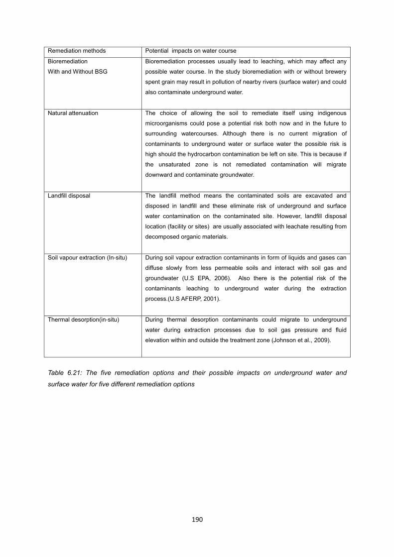
190
Remediation methods Potential impacts on water course
Bioremediation
With and Without BSG
Bioremediation processes usually lead to leaching, which may affect any
possible water course. In the study bioremediation with or without brewery
spent grain may result in pollution of nearby rivers (surface water) and could
also contaminate underground water.
Natural attenuation The choice of allowing the soil to remediate itself using indigenous
microorganisms could pose a potential risk both now and in the future to
surrounding watercourses. Although there is no current migration of
contaminants to underground water or surface water the possible risk is
high should the hydrocarbon contamination be left on site. This is because if
the unsaturated zone is not remediated contamination will migrate
downward and contaminate groundwater.
Landfill disposal
The landfill method means the contaminated soils are excavated and
disposed in landfill and these eliminate risk of underground and surface
water contamination on the contaminated site. However, landfill disposal
location (facility or sites) are usually associated with leachate resulting from
decomposed organic materials.
Soil vapour extraction (In-situ)
During soil vapour extraction contaminants in form of liquids and gases can
diffuse slowly from less permeable soils and interact with soil gas and
groundwater (U.S EPA, 2006). Also there is the potential risk of the
contaminants leaching to underground water during the extraction
process.(U.S AFERP, 2001).
Thermal desorption(in-situ) During thermal desorption contaminants could migrate to underground
water during extraction processes due to soil gas pressure and fluid
elevation within and outside the treatment zone (Johnson et al., 2009).
Table 6.21: The five remediation options and their possible impacts on underground water and
surface water for five different remediation options

191
Remediation methods Potential impacts on land and facility
Bioremediation With and Without BSG
The process could impact surrounding buildings as a result of leachate from
contaminated soil mixing with BSG. There may be potential risk of leachate
to underground facility or water because the tilling and turning of the soil are
carried out above surface. Although any leachate migrating out of the
treatment site are collected and treated see risk assessment table in section
5.1.3 and appendix lV.
Natural attenuation
The process could impact on any facility or land due to the possibility of
leaching. However, the technique is non- intrusive with limited human
interference. But as the technique relies on the indigenous bacteria to
degrade the soil the process will be slow and uncontrollable.
Landfill disposal
The process does not constitutes any negative impacts on the site as the
contaminated soil are excavated and disposed of and new soil are used to fill
the earth.
Soil vapour extraction (In-situ)
The process could be vulnerable to a high risk to the nearby structure and
underground utilities from the high level of the volatile compounds (diesel).
There could be also explosive risk in nearby structure and underground
utilities from high level of volatile organic compounds and risk from direct
contact with soil vapour such as the exposure to utility installation worker to
contaminated soil. (U.S. AFERP, 2001).
Thermal desorption (In-situ)
There is typical concern about geotechnical stability and damage to
foundations, building or underground utilities. However, control measures are
usually in place as cases are dealt with relatively easily on a site-specific
basis (Johnson, et al., 2009).
Table 6.22: The five different remediation options and their possible impacts on land.
6.5.1. Bioremediation with and without BSG effect on land and water pollution
The adoption of a bioremediation technique could result in leachate percolating
through the soil and possibly entering into the nearby water course as a result of
uncontrolled discharge of suspended sediment as indicated in the hypothetical site.
The leaching may contain the organic waste from the BSG and the hydrocarbons
from the soil and water running off the compacted soil may contribute to diffuse

192
pollution as indicated in table 6.21. This assessment is in accordance with (SuRF,
2010) guidelines which indicate that remediation impacts on water may result from
the release of contaminants such as nutrients and dissolved organic carbon which
will impact on the quality of water.
In addition, the benefits of bioremediation include safe operations, facilitated
materials balance and process controllability (U.S. EPA, 2008b). In the study here
the processes were carried out above ground as tilling and turning of the soil are
carried out on the surface but the potential of leaching to occur from the mixture of
BSG and contaminated soil may affect under or above ground water as shown in the
case study site and indicated in table 6.22. However, control measures could be put
in place to collect leachate from the soil, in the form of trenches excavated around
the treatment location to collect any escaping leachate, which is then sent for
treatment. The risk assessment model in section 5.1.3 addresses the potential risk of
leaching from bioremediation in the study.
6.5.2. Natural attenuation effect on land and water pollution
Natural attenuation technology is referred to as intrinsic bioremediation (Borden et al.
1995) because the process relies on the natural assimilative capacities of the ground
to act on the contaminants (Simarro et al. 2013).The technique also relies on
indigenous microorganisms to degrade the contaminants (Suni and Romantschuk,
2004). The process seems slow and uncontrollable as there is limited human
interferences. There would be no damage to the land or aquifer as a result of use of
the technique as it does not involve the use of heavy machinery or chemicals that
may lead to additional burdens on the soil.
However, climate scenarios in the U.K. such as wetter winters, hotter and drier
summers, rising air temperature, increased storminess and heavier rainfall (Hulme et
al. 2002) could have impacts on technique such as natural attenuation. Thus, severe
weather conditions may have damaging effects on soils with potential impacts for
any ground contamination especially shallow untreated contaminated sites as
depicted in this study in that during winter there may be a seasonal rise in
groundwater levels which can bring clean groundwater in contact with the diesel
contaminants. More so, higher intensity rainfall will challenge soil infiltration capacity
and double the risk of soil erosion and spread of the diesel oil beyond the expected

193
area.
Therefore, the remediation method of natural attenuation in the study may result in
water and land pollution although the hypothetical site shows that the contamination
does not affect the saturated zone and the surface water course. However, since the
natural attenuation will take a minimum of 5 years to achieve based on the
remediation schedule in this study there is an increasing risk of contamination from
eroded soil if the environmental conditions change over time for instance flooding
could impact on surface water and contribute to pollution of site drainage water and
the surrounding land.
6.5.3. Landfill disposal effect on land and water pollution
The adoption of landfill remediation may not lead to any water or land pollution within
the site as the soil would be excavated and disposed in a landfill and clean soil
would be used to replace it. The process involves the contaminants being transferred
to a different location. The volume of contaminated soil at the site in Sunderland is
20,000 tonnes and a total of 16 vehicles will require 1,250 trips to dispose of the soil.
In addition topsoil was used to fill the areas of the site where the contaminated soil
has been removed. The dig and dump method does not have any impact on the
water or surrounding buildings but may increase the risk to human health and
environment through traffic accidents and exposure to dust (EA, 2004).
6.5.4. Soil vapour extraction (SVE) effect on land and water pollution
The remediation technique of SVE considered in the study here would remove the
contaminants from the soil and destroy them using an above ground treatment
process. The treated vapour stream would contain undesirable by-products but they
are the products of complete combustion, CO2 and H2O and they can be released to
the atmosphere because the compounds are innocuous (U.S. EPA, 2006) and may
not have an effect on land and water Using SVE involves several mechanisms but
recovery wells are used to capture both liquid and gases and transport them to the
surface facility for treatment. During the engineering process of air injection there is
the possibility of dangerous vapour migration into buildings or underground utilities
but control processes are usually put in place to mitigate against such an
occurrence. More so, vapour treatment facility is usually designed to meet air
194
discharge regulatory requirements however there could be a risk to groundwater
based on the leaching of contaminants from soil during the extraction process.
6.5.5. Thermal desorption effect on land and water pollution
Thermal desorption considered in the study would produce secondary waste streams
including solids, water condensate and oil condensate, each of which may require
analysis to determine the best disposal/recycle options. During the thermal
desorption process there may be the possibility of an explosive risk to nearby
structures and underground utilities from high levels of volatile organics. This is
because the technique would use a non-oxidizing process to vaporize the
hydrocarbon through the application of heat and as a result of drilling the earth. It
may impact the nearby structure with a risk of high level explosions due to the
volatile nature of the contaminants. But these have not been a significant barrier to
in situ thermal desorption techniques as the concerns regarding land and water
pollution are addressed as part of the project implementation process (Johnson et al.
2009).
However, due to the high temperature used to treat the contaminants the treated soil
would be subjected to weight loss as a result of pyrolysis of the petroleum products
in the soil and even soil that does not have petroleum contaminants in the
surrounding treatment zone may lose weight significantly as temperature rises. Thus,
weight loss could be caused by not only moisture evaporation but also by
decomposition of humus materials. In addition there may be some minerals such as
carbonate salts found in the soil, which could be subjected to high temperatures by
the soil vapour extraction technology (Lee et al. 1998). In addition, contaminants can
diffuse slowly from less permeable soil and interact with soil gas and groundwater,
which may occur during pyrolysis (U.S. EPA, 1996a). Thus, there is a potential of
underground water or land pollution as the process generates waste streams such
as spent carbon and condensed water, which may be disposed in landfill.
6.6. Discussion
During remediation of contaminated soils there are a range of environmental impacts
associated with different remediation techniques. For example bioremediation has
been associated with leachate from decomposing organic matter percolating into the
195
soil and possibly into nearby watercourses and the potential release of any micro-
organisms into the wider environment (Komilis and Ham, 2006).
In addition, bioremediation techniques involve the use of heavy machinery such as
excavator/tractors, petrol and diesel-engine motor vehicles. The use of these
machines, poses a major threat to clean air as they emit a wide variety of pollutants
including CO, NOx, VOCs and PM10, which have an increasing impact on air quality
(Defra, 2010).
In the context of soil remediation environmental burdens caused by the remediation
itself includes impacts on resource consumption, energy usage, transportation
emissions, and toxicity (Ellis and Hardley, 2009). Hence in the present study it is
important to establish the magnitude of emissions from the range of remediation
techniques considered in the study and evaluate which technique is more
sustainable if applied under the same conditions. The discussions of the findings are
presented below:
6.6.1. Process and activities emissions
There are two classifications of emissions under review in the study here - process
and activities based emissions. The process based emissions were referred to in the
study as emissions resulting from the diesel contaminants during remediation, which
may be vaporised/volatised or used by micro-organisms and converted to CO2 and
water during remediation. It is emissions that result from the contaminant (diesel)
directly during remediation. Whilst the activities emissions are as a result of the use
of energy or electricity during the period of remediation these include the use of
heavy goods vehicles or heavy machinery during remediation. The activities
emissions were as a result of remediation activities and not from the diesel
contaminants in the soil. These two classifications are discussed below:
6.6.2. Process emissions from bioremediation technique
Soil respiration is an influential component of the biosphere’s carbon cycle as it
makes up about three-quarters of total ecosystem respiration (Law et al. 2001). Soil
respiration is a major aspect of soil-quality and an indicator of soil fertility (Staben et
al. 1997). But the release of CO2 from the soil has been in the front line of intense
studies in recent years, due to its controversial aspect on global warming potentials

196
(Luo et al. 2001). Therefore, measuring soil CO2 respiration is a medium to assess
biological soil fertility. Bioremediation processes involve the degradation of organic
compounds in the soil and may result in CO2 being emitted (Walworth and Reynolds,
1995) especially when it is enhanced by the addition of organic wastes such as BSG
and this may have an impact on the environment.
In a study conducted in the laboratory by Benyahia et al. (2005) using the method of
measuring CO2 based on the standard titrimetric determination of CO2 trapped in a
concentrated NaOH solution, the bioremediation process yielded a much greater
respiration rate and resulted in a reduction of 75% of oil in the soil in 118 days.
In the study here the respirometry experiment was carried out to determine the
volume of CO2 evolved in the presence and absence of BSG. This information was
then used to review the environmental costs associated with the process. It has been
asserted by (Reddy and Adams, 2010) that measuring environmental impacts of
remediation should include metrics such as CO2 emission per unit of treated soil
(tonne/kg), energy per unit treated mass (kWh/kg), air pollution (kg or tonnes), waste
generation (kg/tonnes) and water consumptions (m3 or gallons). In terms of the
calculation of environmental costs there is a need to ascribe actual values to the
various factors costed (Defra, 2008).
The results from the respirometry in the study indicate that addition of BSG results in
higher microbial activity, as indicated by an increase in emissions of CO2, which was
higher than the treatment without BSG this might be expected as the microbes will
break down the spent grain as well as the diesel contaminating the soil.
From the results in this study BSG will be beneficial in terms of its ability to enhance
the bioremediation process but it could result in a greater environmental impact, in
terms of the release of greenhouse gas emissions.
The adoption of the respirometry technique described here could be one means of
ascribing a value to environmental impacts, in terms of the release of CO2. The
quantitative measurement of CO2 can then be added to the social and economic
costs to determine how sustainable a remediation option could be (SURF-2010). The
value of process emissions from bioremediation with and without BSG has been
estimated to be 0.594 TCO2e. and 0.358 TCO2e respectively (Table 6.11).

197
6.6.3. Process emissions from natural attenuation and landfill disposal
CH4 and CO2 are generated in landfill as waste decomposes. In the study here focus
was only on CO2 which was previously calculated as 0.358 TCO2e (Table 6.11). But
landfill gas can also generate economic benefits for the community as it reduces the
need to use more polluting energy from coal and oil when landfill gas is produced.
Whilst CO2 from natural attenuation has been previously calculated from the
anaerobic decomposition of the organic waste to be 0.358 TCO2e (Table 6.11)
6.6.4. Process emissions from SVE and thermal desorption
In the past thermal, chemical and physical treatment methods have failed to
eliminate the pollution problem because these techniques only transfer the pollution
to a new phase such as air pollution. But with the use of a thermal facility such
thermal oxidizer, which is equipped with a heat exchanger and the combustion gas is
used to pre-heat the incoming contaminated gas (FRTR, 1999), means vaporization
is the main mechanism used to enhance recoveries of volatile organic compounds.
Thus, various residuals are usually generated from the process and in the study it
would be hazardous because diesel fuels are certainly hazardous, which would be
condensed to liquid and treated as off-gas. The in situ thermal desorption method
had been designed and implemented and consistently produced more than 95%
mass removal in clay soil (Baker et al. 2008).
Therefore, the thermal oxidation treatment would result in more than 95% destruction
of the contaminants and they would eventually disperse to the atmosphere as CO2
and water. The by-product of this destruction is referred to as the product of
complete combustion, if they are combusted with sufficient oxygen and these
compounds are innocuous and can be discharged directly to the atmosphere
(U.S.EPA, 2006). Using this technology it is assumed that all the CO2 will be
captured and brought to the surface facility as vapour gases and uses recovery wells
to capture both liquid and gases.
The treated vapour stream would contain undesirable by-products but they are the
products of incomplete combustion (U.S.EPA, 2006). Thus, sufficient heating of the
volatile organic compound in the off-gas facility in the presence of oxygen will
convert the VOCs to a harmless end product (AICE, 1993 and Suthersan, 1999).

198
These can be released to the atmosphere as CO2 and water subject to meeting the
requirement of local air discharge regulations (U.S.EPA, 2006).
Thermal oxidation equipment is currently used for destroying contaminants in the
exhaust gas from air strippers and SVE systems (FRTR, 1999). VOCs are thermally
destroyed at temperatures ranging from 600 to 10000C using a solid catalyst. Initially,
the contaminated air is directly pre-heated to reach a temperature necessary to
initiate the catalytic oxidation of the VOCs. Thereafter, the pre-heated VOC-laden air
is passed through a bed of solid catalysts where the VOCs are rapidly oxidized. The
effluent is either discharged or pumped back as a fluid recycling and the VOCs in the
gas stream are completely destroyed (FRTR, 1999).
However the thermal oxidation system could use a chamber system to combust the
VOCs as described in NFESE, (1998) where contaminants are vaporized in the
treatment chamber and swept away by the air stream and as they pass through a
burn chamber they become part of the combustion process and the contaminants
are destroyed. The VOCs actually serve as a form of supplement fuel in the burn
chamber; helping to heat the circulating gas stream (URL7) and emissions from the
chamber in the study here are regarded as part of the activities emission which are
discussed in the next section.
More so, SVE in the study here would adopt a similar technology of catalytic or
thermal oxidation to treat the air stream laden with volatile compounds (VOCs). Heat
recovery equipment would be installed with a thermal oxidation system to pre-heat
the VOC-laden air stream as described in (Suthersan, 1999). Pre-heating the
incoming stream reduces the amount of fuel that is needed to maintain the
combustion temperature as the VOCs would be used as supplementary fuel.
Although low concentration VOCs streams may not have the oxidation energy
required to maintain the combustion temperatures there is a need for other source of
energy. In the case study site the 20,000 kg of diesel contaminants in the soil would
be combusted and used as a supplemental fuel in addition to other sources of
energy to provide energy for the SVE facility. Although, there may be an element of
process emission (VOC’s) associated with thermal desorption and SVE system.
These emissions were considered as minimal in the study because the facility used
to treat the captured gases or liquid as the VOC laden air was captured by a

199
ventilation system, pre-heated, thoroughly mixed and combusted at high
temperature.
In the study emissions resulting from VOC’s were not evaluated for SVE and thermal
desorption rather they were considered as emissions resulting from the use of
energy, which were grouped as part of the activities emissions. Thus, process
emissions were recorded for bioremediation with and without BSG, natural
attenuation and landfill disposal option. The next sections will discuss the emissions
resulting from remediation activities such as transportation and the use of energy to
arrive at the total emissions measured as CO2e.
6.7 Activities emissions from transportation, use of energy and other
remediation activities
Bioremediation with BSG and other remediation options in the study have emissions
resulting from the use of heavy good vehicles and energy from electricity. For
bioremediation with BSG and without BSG, emissions from the use of heavy goods
vehicles and excavator machines for turning and tilling the soil has been estimated in
terms of CO2 (section 6.4.2). The addition of these emissions to other gases such as
CH4 and N2O are converted into their Global Warming potential (GWP). These three
gases represented as a single value allow different emissions from other remediation
methods to be compared using their GWP. The results section of Table 6.11 has
already converted the three gases into CO2e for the different remediation options
including bioremediation with BSG. Figure 6.3 below shows the comparison of the
CO2e of bioremediation with and without BSG to other remediation options
considered in the study such as landfill, natural attenuation, SVE and thermal
desorption.

200
Fig.6.3: Summarises the pollutants value of emission from remediation and activities
for the different remediation options consider in the study with estimation of their
CO2e.
From Fig. 6.3 bioremediation with BSG was slightly higher than bioremediation
without BSG and natural attenuation because of the movement of heavy goods
vehicles used to transport the BSG from Hartlepool to Sunderland. Landfill disposal
and thermal desorption were much higher than bioremediation due to the high
energy demand of the technology and their associated high CO2 emissions.
However, the results of this study were not in agreement with the study of Baker et
al.( 2011) in which life cycle assessments were conducted at five sites where in situ
thermal desorption was compared with SVE and landfill disposal and the values of
CO2, CH4 and N2O were converted as a single value (CO2e) with their GWP. In that
study thermal desorption in each instance had lower overall environmental impacts
and costs. The reasons for the lower environmental impacts of thermal desorption in
the Baker study was that it would require 240 km to dispose of the soil to landfill and
SVE was expected to be completed in 100 years due to the difficulties of
implementing the technology in that particular site, as compared to 3 years in the
study reported here.

201
In the study here thermal desorption was compared to process based technology
such as bioremediation and there are few or no studies that have made this analysis
because of the difficulties of measuring the environmental footprint of
bioremediation. In addition, the traditional methods of SVE and landfill presented in
this study differ from the Baker study in that the distance covered from Hartlepool
was estimated to be 48 km and SVE average completion time in the UK is 3 years
(Defra, 2010). According to the results in this study thermal desorption, landfill
disposal and SVE produced heavy impacts while bioremediation yielded lesser but
different impacts. This makes bioremediation more comparable in terms of
environmental cost and thermal desorption the least favourable environmental
option.
Landfill disposal has higher CO2 emissions compared to other remediation options in
the study including bioremediation with/without BSG, natural attenuation and SVE.
Thermal desorption in the results reported here has higher CO2 compared to landfill
disposal but landfill is associated with CH4 the impact of which is greater on climate
change, over 20 times that of CO2 (EPA, 2010b). This may make landfill disposal
less attractive when compared to bioremediation, natural attenuation and SVE. It
also an indication that economic activities that could lead to higher greenhouse gas
emissions today are likely to have consequences far into the future (Defra/DECC’s,
2011).
6.8 Other conventional air pollutants
There are emissions, which have increasing impacts on urban air quality as a result
of emission from motor vehicles. The effects of these emissions on air quality are
almost entirely due to vehicle exhaust emissions (Atkin, Report 2007). These are
major threats to clean air and are emitted by petrol and diesel-engine motor vehicles
(Defra, 2010). In the study here these pollutants are only applicable to landfill and
bioremediation as they involved the use of motor vehicle to transport contaminated
soil and BSG. Table 6.11 provides summary values of these emissions emitted to the
atmosphere during remediation activities, which include NOx, PM10, PM2.5, CO, NH3
and SO2. According to the EC (2013) humans can be adversely affected by exposure
to air pollutants in ambient air. Due to their health effects the European Union has
developed an extensive body of legislation that established health based standards

202
to limit the values emitted or concentrations in the atmosphere.
In the study here these emissions, which are associated with landfill and
bioremediation methods were measured. Other remediation options such as thermal
desorption and SVE, which emit similar forms of pollutants including CO and some
oxides of substances like sulphur and nitrogen were not calculated as they are
completely or partially eliminated during the remediation process (U.S. EPA, 2006).
For example thermal desorption facility used by AAA Construction and Development
(URL7) used a system of continuous detection air emissions to monitor pollutants
such as CO and substances like sulphur and nitrogen coming from the afterburner
facility to ensure compliance with the limit of the law and eliminate such hazardous
substances. The facility used for thermal desorption is made to follow the ATEX
Directives. ATEX is a conventional name for Directives 94/9/EC of the Europeans
Union for the regulation of equipment intended for use in hazardous area (URL7).
Whilst SVE equipment is subject to regulation of the ATEX Directives and the facility
is expected to meet the emission standard for NH3 and CO, because of the
insignificant nature of the emissions from the engines use to power the SVE facility
the calculations are not considered in the study here.
The landfill disposal option emitted more of these pollutants than bioremediation due
to the distance covered to dispose of the contaminated soil, which was 241,400 km,
whilst bioremediation covered a total distance of 12,070 km, however, these
pollutants should be treated based on their individual merit because of the air quality
standard set by European Commission on the concentration of these pollutants in
the atmosphere. According to the EU Daughter Directive, (EU, 2013) the limit value
of NO2 is 200 µg/m3 in 1 hour and 50 µg/m3 in 24 hours for PM10. The concentration
value for PM2.5 is 25µg /m3 in 1 year and CO is set for 10 µg /m3. The limit value for
SO2 is set for 350 µg /m3 and there is no limit value for NH3 because it is not
regulated by the Directive.
In practice emissions from these pollutants are not considered during remedial
selection but Defra, (2010) recommend that these should be calculated as part of
sustainable remediation. Exceeding EU concentrations due to remediation activities
seems practically impossible but remediation activities such as movement of
vehicles could contribute immensely to the limit values. In the study using HGVs to

203
dispose of the contaminated soil to landfill was estimated to take 1,250 trips from
Sunderland to Hartlepool. Hot exhaust and cold start emission for 1,250 trips using
HGVs diesel engines should be considred, in terms of pollutants emitted from
collection to disposal points. Whilst the bioremediation technique has been estimated
to be 125 trips to deliver the BSG from Hartlepool to Sunderland although the
number of trips is lower compared to landfill but the collection and disposal points
need to be considered in respect of the EU limit value.
In the study here emission values for NOx, PM10, PM2.5, CO, NH3 and SO2 resulting
from the movement of vehicles for transporting BSG are minimal compared to
landfill. But in practice consideration should be given to the location and time of
activities because exceeding these values are based on measurement per m3 in a
particular area and the averaging period depends on the pollutants under
consideration. However, the values of these emissions in the study between
bioremediation with BSG and landfill disposal option are comparable. Despite the
uncertainty of the concentration of these emissions in various locations covered in
this study the total sum of the impacts meant that with regard to overall evaluation of
NOx, PM10, PM2.5, CO, NH3 and SO2, landfill seems to be environmentally the most
undesirable option for removal of the diesel from the site, compared to
bioremediation when vehicle miles covered by the two remediation methods are
considered.
6.9 Water impacts
In the study here the six remediation options considered were in-situ and ex-situ
such as landfill, which entail excavating and transporting the contaminated soil to
designated landfill. Bioremediation with and without BSG and natural attenuation
could significantly alter the ambient aquifer pH and nitrate concentration if there is
migration to the surrounding water course or beyond the treatment zone in the case
of flooding during bioremediation. For instance the mixture of BSG added to the
diesel contaminated soil could migrate to the sub-surface water. In the study here the
soil pH or the relative acidity of the soil was measured in the laboratory in chapter (4)
and the microbe colonies were able to thrive in the soil. This is because a fairly
narrow pH range encourages microbial colonies (U.S. DOE, 1996). This may not be
the case in the hypothetical site model as the soil tested in the laboratory had diesel

204
concentrators of 5,000 mg/kg-1 soil and 10,000 mg/kg-1 soil for experiment (a) and (b)
respectively. However, in the case study site the diesel concentration was previously
estimated to be 20,000 kg in the 10,000 m3 soil and this may pose a potential
environmental hazard if there was leaching to the surrounding water course as
hydrocarbons such as diesel may be expected to have a lower pH with properties of
a weak acid (U.S. DOE, 1996).
There may be little or no impact of thermal desorption on ground water because
heating the soil generally reduces the solubility of the diesel preventing migration to
ground water and the contaminants would be captured as vapour gasses and
brought to the surface for further treatment. The same can be said of SVE where the
contaminants are captured and treated in an off-gas treatment facility without
migrating to underground water.
The landfill disposal option simply moves the contaminants to a different location
without having any impacts on the surrounding water course. However, during
digging or excavation of the soil with heavy machinery there is the possibility that the
soil could be damaged and could lead to a source of water pollution. But this is
normally dealt with as part of implementation process.
When considering in-situ technology Defra, (2010) recommend that potential
contaminants that can significantly alter the pH of the surrounding water course or
beyond the treatment zone should be evaluated. The impacts on water are not
considered in the study reported here as there was not time to investigate this aspect
in detail, future work could include an assessment of the constituents of leachate
generated by the bioremediation process. While the diagnosis of the nature of the
impact of water is an essential prerequisite for successful remediation of
contaminated land, in many cases some type of evaluation will be required prior to
the remediation work. As there are many different types of impacts on water, so there
are many different forms of solution.
6.10 Land impacts
One of the aims of this research is to achieve the clean-up of soil contaminated with
diesel oil and the remediation options considered have been adjudged to be capable
of achieving more than 90 per cent clean-up level. Complete removal of the diesel
205
from the soil with a particular remediation technique may alter the soil organic matter
and lead to biological perturbation. In the study here quantitative values will not be
assigned to any impacts resulting from land as the information required to undertake
such assessment are judged to be site specific to a particular remediation option.
Nevertheless, attempt have been made to clarify the likely significant of the impacts
for selected remediation options.
The bioremediation technique enhanced by the addition of BSG was found to
changes the soil pH (chapter 4) and improved the removal of the diesel from the soil.
Enhanced bioremediation can affect the organic matter and nutrient balance of the
soil, which may lead to a change in the balance of the localised existing ecosystem
functionality. Although toxicity testing was not carried out in the study to determine
the effect of the BSG on the soil, in a study carried out at the University of
Sunderland by Ben-Hamed, (2012) to assess alternative agricultural uses of spent
grains and investigating the effect of BSG on plant growth, found that after twelve
weeks of study the weight of leaves and roots increased with the level of BSG
added. The results did not show any deficiency of plant growth as a result of the
addition of the BSG that may alter the biological status of the soil but further
research is needed to establish the state of the soil biological functions when BSG
are added to soil contaminated with diesel oil as this may affect the organic nutrients
of the soil.
The impacts of natural attenuation on land include the contaminants remaining in the
ambient air for a long time. They are also likely to remain in the sub-surface for
longer due to reliance on natural processes. This may make the condition of natural
attenuation unpredictable because of the potential for contaminant migration, which
may result in secondary emissions heavier than the original impact. In the study here
it may impact on the nearby water course, if there is flooding or possible
underground water migration. The natural attenuation technique could be compared
to bioremediation without the addition of BSG in that both do not have any
amendment added but the latter was enhanced through turning the soil and
maintaining the water holding capacity of the soil. Whilst their impacts have not been
measured for land both has comparable environmental footprints.
The environmental impact of landfill on land is likely to be significant as the physical
properties of the soil are altered by excavating the soil and filling the site with new

206
soil. This is because indiscriminate removal of soil organic matter and organisms
changes the biological state of the soil. The new soil may not possess the excavated
soils ecosystem functionality. But the use of the site in the study is for housing
development and as such replacing with clean soil is unlikely to have a significant
impact on ecosystem functionality.
The environmental impact of SVE has not been recorded in the UK possibly as the
technique is not commonly used as compared to other countries such as The
Netherlands, Germany and U.S. where it is widely used as a mature technology
(Defra, 2010). But a few studies have shown that during vapour extraction air
injection could lead to dangerous vapour migration to buildings and underground
facilities. This impact is not evaluated in the study reported here.
Thermal desorption is a process technology that raises the temperature of the soil
which may encourage a temporary increase in biological activity of the soil. But the
technique could have the potential to damage the soil structure. This is because a
high temperature may impact on the organic matter of the soil and could have a
sterilising effect on the biological activity and consequently on the long term localised
biodiversity (Defra, 2010).
In the U.K. the first two projects that used this technology were in Teddington, a
former gasworks site in which electrical conductive heating, similar to the one
described in this project was used in 2006. The other was in Harwell (U.K.) where
electrical conductive heating was combined with SVE. According to the Defra Report
both projects were successful. However, the present study does not evaluate the
impacts of thermal desorption on land but due to the high temperature used to
capture the gases there could be a sterilizing effect on the soil, which could stunt
biological activity and inhibit ecosystem functionality (Defra, 2010).
6.11 Conclusions
The careful evaluation of remediation methods is important if resources are not to be
wasted and environmental and health risks are to be minimised. In the study here
environmental impacts of using BSG to augment bioremediation was compared to
other remediation methods, such as bioremediation without BSG, landfill, natural
attenuation, SVE and thermal desorption.

207
The results of the CO2 emissions from bioremediation with and without BSG were
monitored over a timeframe and bioremediation with BSG was higher than the
emissions from natural attenuation. In the field these values are expected to be the
same irrespective of the total timeframe for natural attenuation to be achieved due to
the mass balance of CO2. In addition, because BSG is a biodegradable by-product it
is expected to emit CO2 to the atmosphere if used in bioremediation. Hence the
carbon footprints of any bioremediation process using organic waste are expected to
be greater than that of natural attenuation. However, if the biodegradable by-product
was to be landfilled the CO2 would still be emitted.
Thermal desorption was the least environmentally friendly technique followed by
landfill disposal and SVE as compared to bioremediation with BSG in terms of the
amount of CO2 emitted. The reasons for high CO2 from thermal desorption and SVE
was due to the high energy demands of the technologies. The techniques of thermal
desorption and SVE in this study did not generate any CO2 from the process of
remediating the soil as the contaminants were captured, treated and disposed of
safely but the implementation incurred high rates of electricity and fuel consumption.
This evaluation underscores why all inputs in remediation activities and processes
are important and should be calculated during the remediation process.
Landfill disposal also has higher CO2 emissions when compared to bioremediation
with BSG due to the high fuel consumption used by the heavy goods vehicle for the
disposal of the contaminated soil and re-filling of the land. This showed that the
contaminants were moved from one location to another and the activities involved
also generated CO2 and added to the net emissions of CO2 from landfill disposal.
Landfill is also associated with CH4 if the contaminated soil is deposited in the landfill
due to an anaerobic decomposition of the organic matter and the impact of CH4 on
climate change is 20 times greater than CO2 over a 100 year period. Landfill is
associated with other pollutants that affect local air quality such as NOx, PM10, PM2.5,
CO, NH3 and SO2. The overall consideration of these impacts may make landfill
disposal less attractive. In practice these emissions may not be considered, as a
typical site of this nature in the U.K. is usually landfilled due to the short time
required to remediate the site.
The environmental impact of the GHG’s from the results showed that bioremediation
208
with BSG was lower than thermal desorption and SVE but was associated with
different pollutants that affect local air quality. These include pollutants such as NOx,
PM10, PM2.5, CO, NH3 and SO2. Therefore, there is need for future discussion
concerning what constitutes the highest environmental footprint between GHG and
other air quality emissions during remediation selection process. This has become
necessary due to the health effects of these emissions and currently the pollutants
are not often considered when choosing the best method for remediating
contaminated sites. These local air pollutants are associated with bioremediation
with BSG and landfill disposal option and their values in this study are negligible.

209
Chapter 7
DISCUSSION
7.1. Introduction
In the last decade there has been an increased awareness of the impact of
greenhouse gasses on the environment and as such individuals, organisations and
governments have come to realise that emissions of greenhouse gasses need to be
reduced (Loo, 2009). Extensive research has been carried out aimed at explaining
the changes in climate due to greenhouse gasses and to explore the means by
which they can be countered. One of the commonly accepted methods to reduce
climate change is the reduction of the greenhouse gas emissions (Schers, 2006).
Pollutants such as CO2, CH4 and N2O trap the outgoing infrared radiation from the
earth’s surface. This process is often referred to as the greenhouse effect, which
adds to the net energy input of the lower atmosphere and results in regional and
global changes in climate parameters including temperature and rainfall (Rastogi et
al. 2002). Global climate change has been judged to be correlated with the use of
fossil fuel (Ellis and Hardley, 2009) but remediation techniques including landfill
disposal, SVE, natural attenuation, thermal desorption and bioremediation are
associated with different impacts, which may contribute during the process of
removing pollutants from the soil, air and water.
Methods commonly used to clean-up hydrocarbon polluted soil involve heavy
engineering methods which typically offer relatively quick-fix solutions and could be
expensive with high environmental and social impacts (CL: AIRE, 2007 and Defra,
2010). Historically in the U.K. and elsewhere soils contaminated with hydrocarbons
are usually disposed of to landfill. But this technique cannot be viewed as
sustainable due to its high environmental footprint. There is also legislation from
the European Union and U.K. government which sets targets for the reduction of
biodegradable and hazardous wastes going to landfill and there has been a
decrease in the number of landfill sites that will accept hazardous waste such as
hydrocarbons. This has resulted in fewer landfill sites and higher landfill tax to
dispose of contaminated soils which are normally classified as hazardous waste.
As such legislative and economic drivers have driven the need for alternative options

210
for the clean-up of polluted land and bioremediation is an increasingly popular
option. Bioremediation optimizes the biological system already present in the soil
and degrades the contaminants to an innocuous end or harmless product (Hamby,
1996). The technique is thought to be safe, reliable and environmentally friendly
because it relies on the natural assimilative capacities of the soil to breakdown the
contaminants (Nichols and Venosa, 2008).
However, the breakdown process can be slow. As it relies on the indigenous
microorganisms to degrade the contaminants there is t a need to improve the natural
breakdown processes by the addition of nutrients or other growth limiting co-
substrates not normally present in sufficient quantity in the soil. Nutrients normally
added could be organic or inorganic. Organic wastes could be a source of both
nutrients and microorganisms to improve upon the breakdown of the hydrocarbon
polluted soil (Walworth et al. 2003). Utilizing biodegradable waste in this manner
would divert the waste stream from landfill. BSG is a by-product from the brewery
processes with high water and nutrient content (Thomas and Rahman, 2006). It is
currently disposed of as an animal feed. However, the amount generated means that
the demand for the product is not as high as the volume produced.
However, using organic wastes/by-products, including BSG, to augment the
bioremediation process may be associated with potential environmental impacts.
These could include leachate from the decomposing organic matter that may
percolate through the soil and possible release of microorganisms into the
atmosphere (Komolis and Ham, 2006). In addition, the bioremediation process may
involve movement of vehicles to transport the BSG from the brewery to the
contaminated site and this could result in emissions of CO2. As such the technique
may not be economically feasible or as environmentally friendly as initially thought.
In addition, the costs of not developing the land, as the time taken for the
bioremediation target to be achieved may be greater, than adopting other quicker
methods such as landfill.
In order to achieve sustainable remediation the impacts of a given remediation
option should not be more than leaving the contaminants untreated. Hence in the
present study it is important to balance the economic, social and environmental
impacts of using BSG to remediate contaminated soil with diesel. Since a discussion

211
of the results obtained has been presented at the end of each chapter, this final
discussion will give an overview of the study and draw attention to the main findings.
7.2. Does the addition of BSG improve the bioremediation of hydrocarbon
contaminated soil?
The results of both experiments carried out for the study reported here, showed a
reduction of 95% in diesel contamination was achieved in 104 days in experiment (2)
and 60 days in experiment (1) after the addition of BSG as compared to the
treatment without BSG, which recorded 91% in experiment (2) and 72% in
experiment (1) respectively.
The microbiological results showed the hydrocarbon utilizing bacteria in soil
amended with BSG were appreciably higher compared to those without the BSG.
The likely reason for this is that BSG is known to have a high nitrogen content
(Thomas and Rahman, 2006) and is a necessary nutrient for bacteria biodegradative
activities. It has also been reported in other studies that there are high quantities of
nitrogen and phosphorus in organic wastes, with appreciable quantities of nitrogen in
BSG (Abioye et al. 2012 and Joo et al. 2007) and this can then be a limiting factor in
the bioremediation of hydrocarbon contaminated soils (Yang, 2009).
The results of the biological and chemical analysis answer the first question of the
research that the use of BSG improved upon the bioremediation of diesel
contaminated soil. However, remediation of contaminated land has been previously
described as being an expensive and technically difficult process and cost is
considered as one of the major drivers of remediation (Euro-Demo, 2006). The
assessment of the total cost of using BSG to remediate contaminated soil was
carried out. In order to achieve this, a case study site was developed. Pollution at the
site was diesel with an approximate volume of 20,000 kg spread over an area of
10,000 m3 and the contaminants were found on the unsaturated area of the site. The
next section discusses the results obtained from the case study site.
7.3 Is the use of bioremediation with BSG economically viable?
In order to calculate the actual cost of using BSG to remediate diesel contaminated
soil a case study site was developed. The purpose of remediating the site was to
build 300 new homes for residential purposes. The site preliminary conceptual model
212
in chapter 5 highlights the potential sources of contaminants, pathways and
receptors.
To determine the economic costs of using the BSG to remediate the soil all costs
associated with the processes were evaluated including direct and indirect costs.
There is a need to compare the economic cost of using BSG to remediate the soil
taking ‘time’ into consideration and making comparisons to other remediation options
such as landfill, natural attenuation, SVE and thermal desorption, which are used in
the U.K. and elsewhere.
The timeframe for the remediation objective to be realised in the field, using BSG
has been estimated to be six months (chapter 5) and this timeframe was used when
estimating indirect economic costs associated with delayed development at the site.
There are limited studies that address the ‘true’ cost of remediation of contaminated
land, as cost is a site specific issue (Defra, 2010).The true costs of remediation are
not often calculated by remediation practitioners because costs relating to one site
may not be applicable to other sites meaning that decisions as to the choice of
remediation technique to be used may not be based upon accurate and realistic
costings.
The cost of using BSG to remediate the soil was calculated including the direct and
indirect costs associated with the technique. The direct cost is the actual costs that
can easily be quantified because they have market value. Whilst indirect costs could
be described as costs that reflect activities that indirectly induce costs during the
period of remediation, such as the time scale it takes to achieve the remediation
objective and other hidden costs that are not normally considered during the
remedial selection process. Categorising costs in this manner will allow remediation
practitioners to build safe, durable and economic structures (Tedd, 2001) and make
an informed decision on the actual remediation costs as this falls into the ethos of
sustainable development.
The total costs of using BSG to augment the bioremediation process in the case
study site showed that bioremediation, with BSG was a viable option and cheaper
than other remediation methods considered in the study. In addition, the results of
the cost model in the study demonstrated how costs are sensitive to certain
213
conditions and could be a function of the purpose of the site, the technology used
and the duration of the remediation works.
However, economic cost is only one strand of sustainability. Hence there is need to
investigate the environmental cost of using BSG to augment the bioremediation
process.
7.4. What are the environmental costs of bioremediation using BSG?
Historically, the major concerns in selecting a remediation technique in the UK have
been costs and feasibility (CL: AIRE, 2006). This is beginning to change with greater
appreciation of environmental and social impacts and the consideration of these
elements would be valuable in the design of a sustainable remediation project. The
case study site presented here compared the environmental cost of bioremediation,
with the use of the BSG, with other remediation options such as landfill disposal,
natural attenuation,SVE and thermal desorption.
As the bioremediation process relies on the optimization of indigenous
microorganisms to break down the contaminants, diesel will be broken down and
released as CO2 and water. This will generate emissions that will affect climate
change with global warming potentials. More so, the use of heavy goods vehicles to
transport the BSG and the use of heavy machinery for tilling and turning the soil
during bioremediation activities will result in emissions to atmosphere.
Whilst finding the most suitable technology for the remediation of a contaminated
site, environmental sustainability of the chosen technology is becoming an important
consideration. However, it is far more difficult to evaluate environmental costs, as
compared to economic costs, due to the difficulties of ascribing financial values to
environmental impacts and the inability to arrive at accurate figures. Hence for many
remediation projects environmental evaluations are not considered and in situations
where evaluation is carried out various values are derived from different assessors,
even when the projects are of the same nature. For example a group of practitioners
in the remediation industry were surveyed in the U.K., and it was found that most of
them evaluated their environmental sustainability differently using various techniques
and matrices and they did not adhere to a particular approach (SuRF-U.K, 2010).
Reddy and Adams, (2010) asserted that there is no universally accepted way of

214
calculating the environmental elements including CO2 and other environmental
footprints and this has led to an array of carbon calculators that have been
developed over the past few years creating confusion and inaccurate information. An
attempt to measure emissions associated with bioremediation, with the use of BSG,
has been carried out in this thesis. A laboratory experiment was conducted to
determine the CO2 associated with bioremediation methods and the measurement of
all the environmental impacts including land and water media and the results were
compared to other remediation options considered in the study.
Table 7.1 below shows the overall impacts on each of the environmental media.
Media
Overall impacts (most impacted)
Overall impacts (less impacted)
Air pollution
Thermal desorption, landfill and soil vapour extraction
Bioremediation with and without BSG and natural attenuation
Water pollution
Bioremediation with and without BSG and natural attenuation
Soil vapour extraction and thermal desorption
Land pollution
Natural attenuation, soil vapour extraction and thermal desorption
Bioremediation and landfill
Table 7.1 The overall impacts on the three media of air, water and land pollution.
From the results in Table 7.1 air emissions involved the quantitative evaluation of the
impacts of the six remediation options and values were ascribed to the emissions
and comparisons were made amongst the different remediation methods. It was
found that natural attenuation was the most environmentally friendly followed by
bioremediation without and with BSG. Thermal desorption was the least
environmentally friendly option. SVE and landfill disposal options were higher in
terms of environmental cost than bioremediation with BSG. This valuation was based
on the amount of greenhouse gases emitted by each remediation technique.
There were other pollutant emissions that affect local air quality and these emissions

215
were only associated with landfill and bioremediation with BSG, due to the use of
heavy good vehicles to transport the diesel contaminated soil and the transportation
of the BSG from one location to another. The pollutants include CO, NOx, VOCs and
PM10. These emissions are not normally considered in practice during selection,
design and implementation of sustainable remediation technologies at contaminated
sites and incorporating these elements will pave a way to determine which air
pollutants should be considered.
Water and land media were assessed qualitatively without ascribing values to their
impacts. This highlights the problem of assigning values to all environmental media.
There is a need for accurate costing models that cut across the three environmental
media.
The work presented in this study has shown the evaluation of six different
remediation methods qualitatively and quantitatively. The evaluation was based on
economic feasibility and the environmental cost of implementing the different
technologies. A comparative assessment of bioremediation and other remediation
techniques showed that bioremediation, with BSG, seems promising as compared to
other options due to its low economic costs and reduced environmental impact.
But will these meet the criteria of sustainable remediation without taking into
consideration the social strand of sustainability? The next section will introduce this
social element.
7.5. What are the social elements of the use of BSG to remediate diesel
contaminated soil?
The social element of remediation according to SuRF-UK, (2010) are actions that
impacts on human health and safety, ethical equity considerations, impacts on
neighbourhoods or regions, community involvement and satisfaction, compliance
with policy objectives and strategies and uncertainty. These are regarded as social
indicators that should be measured during remediation of groundwater and land
contamination.
The social focus with the use of BSG to remediate diesel contaminated land would
involve risks to site workers, neighbours and the public from remediation work
including hazardous process emissions such a PM10 and PM2.5, noise, odour, dust,

216
and chemical exposure of the diesel contaminants (as it was carried out above
ground) during excavation and turning of the soil by heavy machinery.
The social impacts resulting from the movement of heavy goods vehicles to deliver
the 2,000 tonnes of BSG to the site and the impacts of traffic within the locality
should be considered. These impacts according to the guidelines in (SuRF-UK,
2010) should be measured if the remediation activities may have an effect on
neighbourhoods. Different remediation technologies are associated with different
levels of impact that will affect community satisfaction.
In the study here the social element may also include benefits such as the use of
minimal water during remediation and the use of recycled by-product material, which
is an alternative option to disposing of the by-product. These benefits and other
impacts mentioned above would be compared to other remediation options
considered in the study to determine which option is most sustainable when
remediating diesel contaminated soil. Hence there is need to evaluate the social
elements of all of the remediation methods considered in this study, however, due to
time constraints the social strand was not evaluated, but it is an area of concern that
should be addressed. The expected social benefits of using BSG to augment
bioremediation include:
The process encourages the re-use of by product material.
The process diverts BSG from landfill if it is not being used as
feedstock.
Minimize risk to site workers and neighbours through reduced
movement of heavy goods vehicles when compared to landfill.
Noise level is minimal compared to other methods such as SVE and
thermal desorption.
There is a reduction in emissions compared to other options in the
study.
Minimal uses of water compared to other remediation options such as
thermal desorption and SVE.

217
Land is put into alternative use as the project provides affordable
houses and re-generates the area with 300 new homes.
Therefore, sustainable remediation aims to balance the remediation practices,
processes, and technologies with the need to use less energy and resources, reduce
emissions, without negative impacts on the lives of occupants, neighbours, and
ecosystems during the implementation of the remediation techniques (Gimpelson,
2011). Various qualitative and quantitative analytical methods can be used to provide
the neccessary information and sustainable remediation methods, which entail
balancing multiple factors to create a holistic assessment of each method to select
the one that provides the greatest benefit for all.

218
Chapter 8
CONCLUSIONS
8.1 Introduction
The work presented in this study has shown that the addition of BSG has resulted in
the bioremediation of diesel contaminated soil and breakdown of the diesel by 95%
(concentration 3,400 mg kg-1) over 60 days and 95% (concentration 68,000 mg kg-1)
over 104 days. It also showed that the technique is an economically viable option
with reduced environmental costs. A comparative assessment of bioremediation and
other remediation techniques in the study showed that bioremediation with BSG
seems promising due to its low economic and environmental costs. The evaluation
was based on economic feasibility and the environmental cost of implementing the
different technologies.
Amongst the remediation options considered natural attenuation was an attractive
remediation technique in the study but there was a high economic cost associated
with not developing the site coupled with cumulative impacts that would occur during
its characteristic long duration. The same can be said of the SVE technique, which
has a long duration to achieve the remediation objective and high economic costs
due to the likelihood of the SVE system being unable to extract some diesel
components. SVE and thermal desorption techniques are technologies that
encourage controlled contaminant partitioning between the environmental media in
that contaminants are moved from soil to liquid or from liquid to air.
The excavation and disposal option will result in immediate and long term emissions
due to emissions from heavy goods vehicles to transport the contaminated soil from
one location to another (immediate) and the breakdown of the contaminants in the
landfill site (long-term) will generate CH4. In addition, the impact of CH4 on climate
change is over 20 times that of CO2 over a 100 year period.
Remediation technologies such as bioremediation have been identified in the study
as needing a low energy input and shorter treatment time due to the augmentation of
the BSG to speed up the process.

219
Summary of key findings:
The economic and environmental impacts of remediating the soil using
BSG to augment the bioremediation process is less than the impacts
of leaving the site untreated.
It is a technology that promotes the re-use and utilization of by-product
materials such as BSG.
It is a technique that reduces energy consumption associated with site
remediation.
The bioremediation processes minimize the risk to public health and
the environment in a cost-effective manner and at a reasonable time
frame compared to other options.
It minimizes the emission of air pollution and GHGs and minimizes
impacts to land and ecosystems.
8.2 Recommendation for future work
There is need for the technology to be transferred to the field in order to demonstrate
the practicality of the technique.
Other future work needed includes:
The bioremediation process of using BSG was successful in the laboratory but there
is need for field scale trials across a range of soil types.
There is also a need to obtain accurate quantitative values for
environmental impacts for water and land.
The addition of BSG may bring with it other micro-organisms and
nutrients. This needs to be investigated.
There is a need to investigate the CO2 released from the BSG itself
during the bioremediation process.
There is need to measure the social element of sustainability in order
to have a holistic assessment of the bioremediation process.

220
In terms of sustainable remediation there is a need to develop
indicators for the social impacts.
The results of this study showed that thermal desorption was the least
environmentally friendly option. Bioremediation and natural attenuation were the
most environmentally friendly method. SVE and landfill disposal option were higher
in terms of environmental costs than bioremediation with BSG. This valuation was
based on the amount of greenhouse gas emitted by each remediation techniques.
However, the results of the potential impacts on other media, such as land and
water, indicate that the six remediation technologies do have environment impacts
with variations with each media.

221
9. References
• Abioye, O.P., Agamuthu, P. and Abdul Aziz, A.R. (2012) Biodegradation of
Used motor oil in soil using organic waste amendments. Biotechnology
research international 2012, pp.1 – 8.
• Adekunle, I. M. (2011) Bioremediation of soils contaminated with Nigeria
petroleum products using composted municipal wastes. Bioremediation
Journal, 15, pp.230-241.
• Adesodun, J. K., Davidson, D. A., and Mbagwu, J. S. C .( 2007) ‘Soil Faunal
activity of an oil-polluted tropical alfisol amended with organic wastes as
determine by micromorphological observations’. Applied Soil Ecology 39, pp
46-57.
• Adesodun, J. K. and Mbagwu, J. S. C. (2008) ‘Bioremediation of wastes-
lubricating petroleum oil in a tropical alfilso as mediated by animal droppings’.
Bioresource Technology 99, pp 5659-5665.
• Admon, S. Green, M., Avnimelech, Y. (2001) Biodegradation kinetics of
hydrocarbons in soil during land treatment of oily sludge. Bioremediation
Journal, (5), pp.193-209.
• Ali, A. and Dahot, M.U. (2009) Characterization of crude alkaline protease of
soybean seeds. Sindh Univ. Res. Journ. (Sci.Ser), 41,(2), pp.7-14.
• Ali, S. and Bala, M. (2011) Brewer’s spent grain: A review of its potentials and
applications. Africa Journal of biotechnology, 10(3), pp.324-331.
• Al-Mutairi N., Bufarsan., Al-Rukaibi. (2008) Ecorisk evaluation and treatability
potential of soil contaminated with petroleum hydrocarbon-bases fuels.
Chemosphere 74. pp 142-148.
• Ameh, A. O., Mohammed-Dabo, I.A., Ibrahim, S., Ameh, J. B., Tanimu, Y.,
and Bello, T. K. (2012) Effect of earthworm inoculation on the bioremediation
of used engine oil contaminsted soil. Int. Journal Biol. Chem. Sci. 6(1),
pp.493-503.
• American Institutes of Chemical Engineers (AICE) (1993) Reducing and
222
controlling volatile organic compounds. Centre for Waste Reduction
Technologies, New York.
• American petroleum institutes, (1983) Land treatment practice in the
petroleum industry, report prepared by environmental research technology
Inc. Washington, DC.
• Andreottola, G., Dallago, L., and Ferrarese. ( 2008) Feasibility study for the
remediation of groundwater contaminated by organolead compounds. Journal
pf Hazardous Materials, 156, pp.488-498.
• Atkins report, (2007) Development of hazardous waste pre-treatment: final
report. Job No. 5050571.
• Atkinson G. and Diock, T. (2010) Brownfield land regeneration to
Greenspace: improving the sustainability credential of regeneration project
through process modelling.
• Balba, M. T., Al-Awadhi, N., and AL-Daher, R. (1998) Bioremediation of oil-
contaminated soil: microbialogical methods for feasibility assessment and field
evaluation; Journal of microbiological methods. 32, pp.155-164.
• Barbie, E.B. (2000) Valuing the environment as input: review of application to
mangrove-fishery linkage. Ecological economics. 35, pp.47-61.
• Baker, R.S., Bierschenk, J.M., LaChance, J., Galigan, J.P., and Tarmasiewicz,
D. (2008) Why In Situ thermal desorption can be the most cost-effective
remediation method for many sites. Battlle press, Columbus, OH.
• Baker, R.S., Burdett, T., Nelson, S.G., Faubye, M., Ploug, N., and Holm, J.
(2011) Sustainable remediation state practice. International Conference
University of Massachusetts Amherst.
• Barthe, R. (1986) Biotechnology of petroleum pollutant biodegradation.
Microbiology Ecology, 12, pp.155-172.
• Ben-hamed U. (2012) An analysis of the use of brewery spent grain : a case
study of the U.K. brewery industry. Thesis (Ph.D) at University of Sunderland.
Ethos ID: uk.bl.ethos 556491.

223
• Bento, F. M., Camango, F. A. O., Okeke, B. C., Franken Berger, W. T. (2005)
‘Comparative bioremediation of soil contaminated with diesel oil by natural
attenuation, biostimulation and bioagmentation’. Bioresource Technology 96,
pp.1049-1055.
• Benyahia, F., Abdulkarim, Chaalal, Z. O., and Hasanain, H. (2005)
Bioremediation of crude oil contaminated soils- A Black Art or an Engineering
Challenge? Institution of Chemical Engineers 83(B4), pp.364-370.
• Bennedsen, M. B., Scott, J.P., and Hartley, J. D. (1985) Use of vapour
extraction system in site removal of volatile organic compounds from soil.
Proceedings of the National conference on hazardous wastes and hazardous
materials, HMCRI. 92-95.
• Bonnieux, F. and Rainelli, P. (1999) Contingent valuation methodology and
EU institutional framework: valuing environmental preference, theory and
practices of the contingent valuation method in US, EU, and developing
Countries, New York Univeristy Press, 585-612.
• Borras, E., Caminal, G., Serra, M., Novotny, C. (2010) Effect of soil bacteria
on the ability of polycyclic aromatic hydrocarbon (PAHs) removal by trameters
versi-colour and irpex lacteus from contaminated soil. Biology and
Biochemistry, 42, pp.2087-2093
• Borden, R.C., Gomez, C.A., and Becker, M.T. (1994) Geochemical indicators
off intrinsic bioremediation. Ground water. 33, 2, pp.181-189.
• Borden, R.C., Gomez, C.A., Becker, M.T. (1995) Geochemical Indicators of
Intrinsic Bioremediation. Ground water 33 No 2 pp.180-186.
• Bostrom, D. (2004) Project Experience with Oxidation System” By Dan
Bostrom, Senior Program Manager. ENSR, 2004c.
• British standard (BS:10172) (2001) Investigation of potentially contaminated
sites- code of practice.
• Cam, D and Gagni, S., (2001) Determination of petroleum hydrocarbons in
contaminated soils using soilid-phase microextraction with gas

224
chromatography-mass spectrometry. Journal of chromatographic science,(
39), pp.481-486.
• Chang, W., Dyen, M., Spagnuolo, L., Simon, P., Whyte, L. and Ghoshal, S.
(2010) Biodegradation of semi- and non-volatile petroleum hydrocarbon in
aged, contaminated soils from a sub-Artic site: Laboratory pilot-scale
experiments at site temperatures. Chemosphere, 80, pp.319-326.
• Cho, B., Chino, H., Tsuji, H., Kunito, T., Nagaoka, K., Otsuka, S., Yamashita,
K., Matsumoto, S., Oyaizu, H. (1997) Laboratory –Scale Bioremediation of
Oil-Contaminated Soil of Kuwait with Soil Amendment Materials.
Chemosphere. 35, (7), pp. 1599-1611.
• Chaudhary, V.K. and Weber., F.E. (1990) Dietary fibre ingredients obtained
by processing brewer’s dried grain. Journal of food science, 55, pp.551-553
• Chen, S.K. Edwards, C.A., Subler, S. (2003) The influence of two agricultural
biostimuation on nitrogen transformation microbial activity, and plant growth in
soil microcosms. Soil Biology and Biochemistry, 35, pp.9-19.
• CH2M-HILL Inc. Reston, VA. (1985) Remediation planning/field investigation
team: Verona well field- Thomas solvent company, battle Creek, Michigan,
operable unit feasibility study.
• Ciric, L., Griffiths, R.I., Philip, J.C. and Whiteley, A.S. (2010) Field scale
molecular analysis for the monitoring of bacteria community structures during
on-site diesel bioremediation. Bioresource Technology,101, pp5235-5241.
• Collins, P.H. (2001) Dictionary of Ecology and the Environmental, Fourth ed.
Peter Collin Publishing, London.
• Contaminated Land: Applications in Real Environments (CL:AIRE),
(2006) Project SIReN: The Site for Innovative Research into Monitored
Natural Attenuation. Subr:im bulletin January 2006.
• Contaminated Land: Applications in Real Environments (CL:AIRE),
(2007) Uncover the true impacts of remediation. Subr:im bulletin sub 2 March
2007.
225
• Contaminated Land: Applications in Real Environments (CL: AIRE),
(2011) In situ radio frequency heating (ISRFH) of hydrocarbon contaminated
chalk at a former service station in Kent, 2011 TDP28.
• Community and Local Government (CLG), (2012) Statistical data set: live
tables on household projections: published on 10 November, 2012.
• Covino, S. Svobodova, K., Cvancarova, M., Annibale, A., Petruccioli, M.,
Federici, F., kresinova, Z., Galli, E. and Cajthaml, T. (2010) Inoculum carrier
and contaminant bioavailability affect fungal degradation performance of PAH-
contaminated solid matrices from a wood preservation plant. Chemosphere,
79, pp.855-864.
• Cropper, M.L. (2000) Has economics research answer the needs of
environmental policy? Journal of Environmental economics and management,
39, pp.328-350.
• Crossno, S.K., Kalbus, L.H., Kalbus, G.E. (1996) Determinations of carbon
dioxide by titration: new experiment for general physical and quantitartive
analysis courses. American Chemical Society, Vol.73(2), pp.175-176.
• Dadrasnia, A. and Agamuthu, P. (2010) Enhanced degradation of diesel-
contaminated soil using organic waste. Malaysia Journal of Science, 29(3),
pp.225-230.
• Dadrasnia, A. and Agamuthu, P. (2013) Organic wastes to enhance phyto-
treatment of diesel-contaminated soil. Waste management resources, 31(11),
pp.1133-1139
• Day, S.J., Morse, G.K., and Lester, J.N. (1997) The cost effectiveness of
contaminated land remediation strategies. Science of total environment, 201,
pp.125-136.
• Deaton, B. J. and Hoehn, J. P. (2004) Hedonic analysis of hazardous waste
sites in the presence of other urban disamenities. Environmental. Science and
Policy, 7, pp.499-508.
• Defra, (2005) Key factors about: waste and recycling. (Available:
226
www.defra.gov.uk).
• Defra, (2006) Environmental Protection Act 1990 : Part 11A, contaminated
land. (Available: www.defra.gov.uk).
• Defra, (2007) Introductory guide to option for division of biodegradable
municipal waste from landfall. (Avalable : www.defra.gov.uk).
• Defra, (2008) Industrial pollution control regimes. ( avalable :
www.defra.gov.uk).
• Defra, (2010) Contaminated land remediation final reports defra research
project. SP1001.
• Defra/WAG, (2010) Simplification of contaminated land statutory guidance.
Impact Assessment IA NO: Defra 1133.
• Defra/DECC’s, (2011) Guidance of GHG conversion factors for company
reporting: methodology paper for emission factors. (Available:
www.defra.gov.uk).
• Defra, (2011) Guidiance on applying the waste hierarchy to hazardous waste.
Published November, 2011, PB13687 (Available: www.defra.gov.uk).
• Department of Transport (DFT), (2010) Reported road casualties in Great
Britain: Main results. Pp.1-4.
• DETR, (2000) Waste Strategy for England and Wales. Départment for the
Environnent, Transport and Régions, HMSO, London.
• Deuel L.E and Holliday G.H. (1994) Soil Remediation for Petroleum
Extraction Industry. Pennwell Publishing Company.
• Dias, R. M., Ruberto, L., Hernandez, E., Vazquez, S. C., Balbo, A. L., Del
Panno, M. T. and Mac Cormack. (2012) Bioremediation of an aged diesel oil-
contaminated Antarctic soil: Evaluation of the site on site biostimuation
strategy using different nutrients sources. International Biodeterioration and
Biodegradation, 75, pp.96-103.
• Dick, W.A. and Tabatabai, M.A. (1992) Potential uses of soil enzymes. In:

227
Metting, B.(ed). Soil Microbial Ecology, Marcel Dekker, New York, pp.95-127.
• Dijkgraaf, E., and Vollebergh, H.R.J. (2004). Burn or Bury? A social cost
comparison of final waste disposal methods. Ecological Economics, 50,
pp.233-247.
• Diplock, E.E., Mardin, D.P., Killham, K.S., and Paton, G.I. (2009) Predicting
bioremediation of hydrocarbons: laboratory to field scale. Environ. Pollution,
57, pp.1831-1840.
• Dixon, T., Raco, M., Catney, P., and Lerner, D. (2007). Sustainable Brownfield
regeneration: Liveable Places from Problem Spaces, Wiley-Blackwell.
• Dixon, T., Otsuka, N. and Abe, H. (2011) Critical success factors in urban
brownfield regeneration: an analysis of hardcore sites in Manchester and
Osaka during the economic recession (2009-10). Environmant and planning
A, 43 (4), pp.961-980.
• EC, (1999) Council Directive of 26 April 1999 on the landfill of waste
(1999/31/Ec). Official Journal of the European Communities L/182/1,
167/1999.
• EC, (2013) Air quality standard. Factsheet clean air for all. (Avialable:
http://ec.europa.eu/environment/air/quality/standards.htm
• Edward-Jones, G., Davis, B., Hussain, S. ( 2000) Ecological economic: an
introduction. Blackwell Science Ltd.
• Ellis, D.E. and Hadley, P.W. (2009) Sustainable remediation white paper-
integrating sustainable principles, practices, and metrics into remediation
projects.
• Environmental Agency (EA), (1999) Cost and benefit Associated with
Remediation of Contaminated Groundwater: A Review of the Issues,
Research and Development: Technical Report p278.
• Environmental Agency (EA), (2004). Mobilising nature’s armoury: monitored
natural attenuation- dealing with pollution using natural processes. British
Geological survey. IPR/42-21C.

228
• Environmental Agency (EA), (2005) The UK approach for evaluating human
health risks from petroleum hydrocarbons in soils. Science report p5-080/tr3.
• Environmental Agency (EA), (2010a) Remediation position statements.
Operational instruction. Version 3. Doc.No. 226-06.
• Environmental Agency (EA), (2010b) Verification of remediation of land
contamination. Report: Sc030114/R1.
• European Co-ordination Action Demonstration (Euro-Demo), (2006)
European platform for demonstration of efficient soil and groundwater
remediation. Report on case studies. Project No. (GOCE) 003985. Available:
http://www.eurodemo.info/
• European Groundwater and Contaminated Land Remediation
Information System (EUGRIS), (2012) Is a web-based information platform
for contaminated land and groundwater. Available : http://www.eugris.info
(accessed on the 12th of March, 2012).
• Fountoulakis, M.S., Terzakis, S., Kalogerakis, N. and Manios, T., (2009)
Removal of polycyclic aromatic hydrocarbons and linear alkylbenzene
sulfonates from domestic wastewater in pilot constructed wetland and a gravel
filter. Ecological Engineering, 33, pp.1702-1709.
• Federal Remedaition Technology Roundtable (FRTR), (1999) Common
treatment technologies for non-halogenated VOCs. Available on:
http://www.environmental-expert.com/articles/common-treatment-
technologies-for-nonhalogenated-vocs-860
• Federal Remediation Technology Roundtable (FRTR), (2012) Remediation
technologies screening matrix and reference guide, version 4.0. Soil vapour
extraction. Avialable on : http://www.frtr.gov/matrix2/section4/4-7.html.
• Ferguson, S.H., Powell, S.M., Snape, L., Gibson, J. A. E., Franzmann, P.D.,
(2008) Effect of temperature on the microbial ecology of a hydrocarbon-
contaminated Antartic soil: implication for high temperature remediation. Cold
Region Science Technology, 53, pp.115-129.

229
• Fillaudeau, L., Blanpain-Avet, P., and Daufin, G. (2006) Water, wastewater
and waste management in brewery industries. Cleaner production, 14,
pp.463-471.
• Forssell, P., Kontkanen, H., Schols, H.A., Hinz, S., Eijsink, V.G.H., Treimo, J.,
Robertson, J.A., Waldron, K.W., Faulds, C.B., and Buchert, J. (2008)
Hydrolysis of breweryon spent grain by carbohydrate degrading enzymes.
The institutes of brwerying and distilling, 114, (4), pp.306-314.
• Frantroussi, S.I and Agathos, S.N. (2005) Is bioaugmentation a feasible
strategy for pollutant removal and site remediation. Current Opinion in
Microbiology ,8, pp.268-275.
• Frick, C.M., Farrel, R.E., and Germida, J.J. (1999) Assessment of
phytoremediation as an insitu technique for cleaning oil contaminated sites.
Petroleum technology alliance Canada: Calgary, Canada, pp.88.
• Garcia-Blanco, S., Motelab, M., Venosa, A.D., Suidan, M.T., Lee, K., King,
D.W. (2001) Restoration of the oil-contaminated Saint Lawrence River
shoreline: Bioremediation and Phytoremediation. American petroleum
institutes, Washington DC, pp.303-308.
• Garcial-Gill, J.C., Plaza, C., Soler-Rovira, P., Polo, A. (2000) Long term
effects of municipal soild waste compost application on soil enzyme activities
and microbial biomass. Soil Biology and Biochemestry, 32, pp.1907-1913.
• Geisseler, D. and Horwath. (2008) Regulation of extracellular protease
activity in soil in response to different sources and concentrations of nitrogen
and carbon. Soil biology and biochemistry, 40, pp.3040-3048.
• Ghazali, M.F., AbdulRaham, R.N.Z., Salleh, A.B., Basri, M. (2004)
Biodegradation of hydrocarbons in soil by microbial consortium. International
Biodeterioration and Biodegradation, 54(6), pp.845-852.
• Gimpelson, J.L. (2011) Evaluation criteria to select sustainable remediation
methods. A report of description of case. Available on share on LinkedIn.
• Grace, C., Hart, M. and Brookes, P.P. (2006) Laboratory manual of the soil
230
microbial biomass group. Rothamsted research, pp.1-64
• Glenn, A.R. (1976) Production of extracellular proteins by bacteria. Annual
review of microbiology, 30, pp.41-62.
• Gomez, F. and Sartaj, M. (2013) Field scale ex-situ bioremediation of
petroleum contaminated soil under cold climate conditions. International
Biodeterioration and Biodegradation, 85, pp.375-382.
• Gong, X. (2012) Remediation of weathered petroleum oil-contaminated soil
using a combination of biostimuation and modified fenton oxidation.
International Biodeterioration and Biodegradation, 70, pp.89-95.
• Greenwood, P.F., Wibrow, S., George, S.J., Tibbett, M. (2008) Hydrocarbon
biodegradation and soil microbial community response to repeated oil
exposure. Organic Geochemistry.
• Harbottle., M., Smith, S., Al-Tabbaa., and Guthrie. (2005) Technical
sustainable of brownfield land remediation. Paper presented to the SUBR:IM
Conference.
• Harbottle, M.J. and Al-Tabbaa, A. (2006) Combining stabilisation/solidification
with biodegradation to enhance long-term remediation performance.
Proceeding of the second Iasted International Conferencce on Advance
Technology in the Environmental Field, Lanzarote, pp.222-227.
• Harbottle, M.J., Al-Tabbaa, A., Evans, C.( 2007) A comparison of the
technical sustainability of in-situ stabilization/solidification with disposal to
landfill. Journal of hazardous materials, 141, pp.430-440.
• Haritash, A.K. and Kaushik, C.P. (2009) Biodegradation aspects of polycyclic
aromatic hydrocarbons (PAHs): a review. Journal of Hazardous Material, 169,
pp.1-15
• Hamby, H.M. (1996) Site remediation techniques supporting environmental
restoration activities- a review. The siceience of the total environment, 191,
pp.203-224.
• Harmonised, I. (2005) International conference on harmonisation of technical

231
requirement for registration of pharmaceuticals for humans. Validation of
analyte procedure: Text and methodology, Q2 (R)
• Head, I. M. (1998) Bioremediation: towards a credible technology.
Microbiology, 144, pp.599-608.
• Hendershot, W.H. and Lalande, H. (1993) Soil reaction and exchangeable
acidity. In: Carter, M.R. (Ed), Soil sampling and method of analysis. Canada
Society of Soil Science, Lewis Publishers, Borca Raton USA.
• Heron, G., LaChance, J., Bierschenk, J., Parker, K., Vinci, S., Woodmanese,
R., and Scneider, J. (2012) Combining Thermal Treatment with MNA at a
Brownfield DNAPL Site. U.S.A.
• Hickman, Z.A. and Reid, B.J. (2008) The co-application of earthworm
(Dendrobaena veneta) and compost to increase hydrocarbon losses from
diesel contaminated soils. Environmental International, pp.1-2.
• Hiester, U., Schrenk., V., and Weiss. T. (2002) Environmental balancing of
cold SVE and Thermally enhanced soil vapour extraction- practical support for
decision makers. Institutes of hydraulic engineering, University of Stuttgart.
• HM Treasury (HMTG): The Green Book. (2011) Appraisal and Evaluation in
Central Government. Treasury Guidance, London:TSO.
• Houde, A., Kawakami, H.S., Stern, A. and Zhou, G. (1997) Material and
process for separating carbon dioxide from methane. Gas Research Institutes
USA.
• Huang, L., Xie, J., Lv, Y. B., Shi, X., Li, G., Liang, F. and Lian, J. (2013)
Optimization of nutrient component for diesel oil degradation by Acinetobacter
beijerinckii ZRS. Marine Pollution Bulletin, vol.76, pp.325-332.
• Hulme, M., Jenkins, G.J. Lu, X., Turnpenny, J. R., Mitchell, T.D., Jones, R.G.,
Lowe, J., Murphy, J.M., Hassell, D., Boorman, P., McDonald, R. and Hill, S.
(2002) Climate change scenarios for the United Kingdom: the UKCIP02
Scientific Report. Tyndall Centre for Climate Change Research.
• Hutzler, N.J., Murphy, B.E., and Gierke, J.S. (1998) State of technology
232
review soil vapour extraction system. E.P.A. Hazardous Waste Eng. Res.
Lab., Cincinnati, OH.
• Ihlandfeldt, K.R. and Taylor, L.O. (2004) Externality effects of small-scale
hazardous waste sites: evidence from urban commercial property markets
Environmental economic management, 47, pp.117-139.
• Intergovernmental Panel on Climate Change (IPCC), (1995) IPCC Second
assessment-climate change: a report of the intergovernmental panel on
climate change. Cambridge University press, Cambridge.
• Intergovernmental Panel on Climate Change (IPCC), (2006) IPCC
Guidelines for national greenhouse gas inventories, Vol.1-5
• Intergovernmental Panel on Climate Change (IPCC), (2007) Fourth
assessment report: Climate change 2007. Intergovernmental panel on
Climate Change. Cambridge University Press. Cambridge.
• Jackson, T. and Robert, P. (2000) A review of indicators of sustainable
development: A report for Scottish Enterprise Tayside. Geddes centre for
planning research.
• Johnson, P. Dahlen, P., and Triplett, J. (2009) Critical evaluation of state of
the art in situ thermal treatment technique for DNAPL source zone treatment.
ESTCP project ER-0314.
• Joo, H.S. Phae, C.G., and Shoda, M. (2007) Degradation of diesel oil in soil
using a food waste composting process. Biodegradation, 18, (.5), pp.597-607.
• Jorgensen, K.S., Puustinen, J., and Suortti. (2000) Bioremediation of
petroleum hydrocarbon-contaminated soil by composting in biopiles.
Environmental Pollution, 107, pp.245-254.
• Juhaasz, A., Stanley, G. A., Britz, M.L. (2000) Degradation of high molecular
weight PAHs in contaminated soil by a bacterial consortium: effects on
Microtox and mutagenicity bioassays. Bioremed. J. 4, pp. 271-283.
• Kaplan, C.W. and Kitts, C.L. (2004) Bacterial succession in a petroleum land
treatment unit. Applied environmental microbiology, 70(3), pp.1777.

233
• Kauppi, S. Sinkkeonen, A., Romantschuk, M. (2011) Enhancing
bioremediation of diesel fuel contaminated soil in a boreal climate:
composition of biostimulation and bioaugmentation. International
Biodeterioration and biodegradation,65, pp.359-368.
• Keller-Reinspach, H.W. (1992) Residues and waste from brewery plants,
possibilities for recycling and disposal. Brauwelt international, 3, 287-293.
• Kiel, K.A. and Zabel, J. (2001) Estimating the economic benefits of clean up
superfund sites: the case of Woburn, Massachussetts. Real estate finance
economic, 2, pp.163-184.
• Kim, S., Choi, D. H., Sim, D. S., Oh, Y. (2005) Evaluation of bioremediation
effectiveness on crude oil-contaminated sand. Chemosphere 59, pp. 845-852.
• Komilis, D.P. Ham, R.K. (2006) Carbon dioxide and ammonia emissions
during composting of mixed paper, yard waste and food waste management
26, pp.62-70.
• Kroeger, T. and Manalo, P. (2006) A review of the economic benefits of
species and habitat conservation. Report prepared for Doris duke charitable
foundation. Washington DC: Conservation Program, Defenders of Wildlife.
• Krummrich, W.G. (2011) 100% Design- thermally enhanced soil vapour
extraction system strategic environmental solution.
• Kumar, C.G. and Takagi., H. (1999) Microbial alkaline proteases: from a
bioindustries viewpoint. Biotechnology Advances,17, pp.561-594.
• Law, B.E., Thornton, P., Irvine, J., Van Tuyl, S., and Anthoni, P. (2001) Carbon
storage and fluxes in ponderosa pine forests at different development stages.
Global Changes Biol, (7), pp.755-777.
• Lee, J.K., Park, D., Kim, B., Dong, J., and Lee, S. (1998) Remediation of
petroleum contaminated soils by fluidized thermal desorption. Waste
Management, 18, pp.503-507.
• Lee, J., Kwon, T., Cho, Y., Kang, H and Jung, W. (2011) Application of
Bioremediation to soil contaminated by Lubricants Around Railroad Turnouts.

234
International Journal of Railway, 4, (1), pp.1-4.
• Lee, M., WOO, S. and Ten, L. N. (2012) Characterization of novel diesel-
degrading strains Acinetobacter haemolyticus MJ01 and Acinetobacter
johnsonii MJ4 isolated from oil-contaminated soil. World Journal Microbiology
Biotechnology, 28, pp.2057-2067
• Levic, J., Sredanovic, S., and Levic, L. (2006) New feeds from brewery by-
product. Romanian Society of Biological Sciences, 11, (.2), pp.2611-2618.
• Liebeg, E.W. Cutright, T.J. (1999) The investigation of enhanced
bioremediation through the addition of macro and micro nutrients in a PAH
contaminated soil. International Biodeterioration and Biodegradation 44, pp.
55-64..
• Liu, P. W., Chang, T.C., Whang, L.M. and Kao, C.H. (2011) Bioremediation of
petroleum hydrocarbon contaminated soil: Effects of strategies and microbial
community shift. International Biodeterioration and Biodegradation, 65,
pp.1119-1127.
• Llado, S., Solanas, A.M., Lapuente, J., Borras, M. and Vinas, M. (2012) A
diversifield approach to evaluate biostimulation and bioaugmentation
strategies for heavy-oil contaminated soil. Science of the Total
Environmental,435-436, pp.262-269.
• Loo, T. (2009) A methodology for calculating CO2 emissions from transport
and an evaluation of the impact of European Union emission regulation.
• Luo, Y., Wan, S., Hui, D., and Wallace, L.L. (2001) Acclimatization of soil
respiration to warming in a tall grases prairie, Nature, (413), pp.622-625
• Love, P.E.D. (2002) Auditing the indirect consequences of rework in
construction: a case based approach. Managerial Auditing Journal, 17 (3),
pp.138-146.
• Maila, M.P. and Cleote, T.E. (2005) Bioremediation of petroleum
hydrocarbons through landfarming: Are simplicity and cost-effective the only
advantages? Review in Environmental Science and Bio/technology,3, pp.349-
235
360.
• Manssfield, R.M. and Moohan, J.A.J. (2002) The evaluation of land
remediation methods. Land Contamination and Reclamation,10(1).
• Margesin, R. (2000) Potential of cold-adapted microorganisms for
bioremediation of polluted alpine soils. International bio deterioration and
biodegradation,46, pp.3-10.
• Margesin, R. Schinner, F. (1997) Bioremediation of diesel-oil-contaminated
alpine soils at low temperatures. Appl Microbial Biotechno. 47 pp.462-468.
• Margesin, R. and Schinner, F. (1999) Biological decontamination of oil spills
in cold environments. Journal of Chemical Technology and Biotechnology, 74,
pp.1-9.
• Margesin, R and Schinner, F. (2001) Biodegradation and bioremediation of
hydrocarbons in extreme environments. Applied microbiology biotechnol, 56,
pp.650-663.
• McEntee, J. (1991) Recycling derelict land, site investigation, edited by
George Fleming, Institution of Civil Engineers, Thomas Telford Ltd.
• McKinnon, A.C. and Piecyk.. (2009) Measurement of C02 emission from
road freight transport: A review of UK experience. Energy Policy, 37, pp.3733-
3742.
• McMahon, V., Garg, B., Aidred, D., Hobb, G., Smith, R., Tothill, I.E. (2008)
‘composting and bioremediation process evaluation of wood waste materials
generated from the construction and demolition indistry’. Chemosphere, 71,
pp.1612-1628.
• Messer, K., Schulze, W., Hackett, K., Cameron, T., and Mcclelland, G. (2000)
Can stigma explain large property value losses? The psychology and
economics of Superfund. Environmental and resources economics, 33,
pp.299-324.
• Miller, H. (1997) The EPA’s war on bioremediation. Nat Biotechnol, 15,
pp.486.
236
• Mittal, A. and Singh, P. (2009) Polycyclic aromatic hydrocarbon degradation
by developed consortium in microcosms study. International Journal of
Microbiology,7,(1).
• Mohamed, S., and Irani, Z. (2002) Developing taxonomies of information
system indirect human costs. Paper presented at the international conference
on system thinking in management, University of Salford, Salford.
• Moon, E. (2003) The development and application of economic valuation
techniques and their use in environmental policy- A survey- Energy transport
and environment, pp.1-34.
• Morales, S.E. and Holben, W.E. (2009) Empirical testing of 16S rRNA Gene
PCR primer pairs reveals variance in target specificity and efficacy not
suggested by In Silico Analysis. Applied and environmental microbiology,
75(9), pp.2677-2683.
• Moreira, I. T. A., Oliveira, O. M. C., Triguis, J. A., Queiroz, A. F. S., Ferreira, S.
L.C., Martin, M.S. C., Silva, A. C. M. and Falcao, B. (2013) Phytoremediation
in mangrove sediment impacted by persistent total petroleum hydrocarbons
(TPH’s) using Avicennia schaueriana. Marine Pollution Bulletin, 67, pp.130-
136.
• Morgan, P. and Watkinson, R. J. (1989) Hydrocarbon degradation in soils and
methods for soil biotreatment. CRC Critical Reviews in Biotechnology, (8),
pp.305-333.
• Muijs, B. and Joner, M.T.O. (2009) Evaluation of clean-up agent for total
petroleum hydrocarbon analysis in biota and sediments. Journal of
chromatography.
• Mussatto, S. I., Dragone, G., Roberto, I. C. (2006) Brewers’ spent grain:
generation, characteristics and potential applications. Review: Journal of
Cereal Science, 43, pp. 1-14.
• National Atmospheric Emission Inventory (NAEI), (2006) Emission
mapping methodology. AEAT/ENV/R/2696.(Available :
naei.defra.gov.uk/index.php)

237
• National Atmospheric Emission Inventory (NAEI), (2008) NAEI UK
mapping methodology. (Available : naei.defra.gov.uk/index.php).
• National Atmospheric Emission Inventory (NAEI), (2012) Road transport
emission factors. (available: http://uk-
air.defra.gov.uk/reports/cat07/1203221052 UK llR 2012 final.pdf).
• Nathanial, J., Bardos, O., Nathanial, P. (2007) Contaminated land
management: Ready reference, land quality press and EPP publication.
• Naval facilities engineering command (NAVFAC), (1998) Application guide
for thermal desorption system. Technical report TR-2090-ENV.
• Naval facilities engineering command (NAVFAC), (2007) Final report- cost
and performance review of electrical resistance heating for source treatment.
Technical report TR-2279-ENV.
• Naval facilities enginerring service centre (NFESC), (1998) Overview of
thermal desorption technology. Contract report CR98.008-ENV. Port
Heeneme, California 93043-4370.
• Nelson, E.C., Water, M.V., Bossert, I.D., Martin, G. (1996) Enhancing
biodegradation of petroleum hydrocarbons with guanidinium fatty acids.
Environmental Sch. And Technol. 30, pp.2406-2411.
• Nichols, W.J. and Venosa, A.D. (2008) Summary of the literature on the use
of commercial bioremediation agents for cleanup of oil-contaminated
environents. International oil spill conference.
• Nikolopoulou, M., Eickenbusch, P., Pasadakis, N. and Venieri, D. (2013)
Microcosm evaluation of autochthonous bioaugmentation to combat marine oil
spills. New biotechnology, vol.30, pp.734-742.
• Nunes, P. A.L. Bergh, V. D., Jeroen, C.J.M., (2001) Economic valuation of
biodiversity: sense or nonsence. Ecological Economics, 39, pp.203-222.
• Owsianiak, M., Lemming, G., Hauschild, M.Z., and Bjerg, P.L.(2012)
Assessing environmental sustainability of remediation technologies in a life
cycle perspective is not so easy. Environmental science and technology.

238
• Paiga, P., Mendes, L., Ailbergaria, J.T., Delurue-Matos, C.M. (2012)
Determination of total petroleum hydrocarbon in soil from different location
using infrared spectrophotometry and gas chromatography. Chemical papers,
66(8), pp.771-721.
• Pagga, U., Beimborn, D.B., Boelens, J., and De Wilde, B. (1995)
Determination of the aerobic biodegradation ability of polymetric material in a
labaoratory controlled composting test. Chemoshere, 31(11), pp.4475-4487.
• Pallant, J. (2007) SPSS Survival Manuel: A step by step guide to data
analysis using Spss for windows 3rd Edition, McGraw Hill: Open University
Press.
• Paul, E.A. and Clark, F.E. (1989) Soil microbiology and biochemistry,
Academic press, New York, pp.46-48.
• Perry, J.J. (1984) Microbial Metabolism of Cyclic Alkanes. In R. M. Atlas (ed.),
Petroleum Microbiology. New York: Macmillan Publishing,. pp.61-98.
• Picado, A., Nogueira, A., Baeta-Hall, L., Mendonca, E., Rodriques, M.F.,
Saagua, M., Martin, A., and Anselmo, M. (2001) Landfarming in PAH-
contaminated soil. Journal of Environmental Science and Health, 36, (69).
• Pollard, S.T., Fisher, J., Twigger-Rose, C. and Brookes, A. (2001)
Approaches to decision support in the context of sustainable development. In
NATO/CCMS Pilot Study, Evaluation of Demonstrated and Emerging
Technologies for the Treatment of Contaminated land and Groundwater
(Phase lll) 200 Special Session, Decision Support Tools, EPA 542-R-01-002.
• Postle, M., Fenn, T., Grosso, A. and Steeds, J. (1999) Cost- benefit analysis
for remediation of land contamination. Environmental Agency Technical
Report P316, December 1999.
• Public works technical bulletin (PWTB), (1999) Biodegradation of
pol.contaminated washrack sludge. U.S. Army Corps of Engineers,
Washington DC. Bulletin 420-49-27.
• Prakash and Irfan, (2011) Pseudomonas aeruginosa is present in crude oil

239
contaminated sites of Barmer region. Journal of bioremediation and
biodegradation 2 (5).
• Prentice, N. and Refsguard, J.M. (1978) Enzymatic hydrolysis of brewers’
spent grain. Journal of the American Society of Brewing Chemists, 36,
pp.196-200.
• Pritchard, H.P. (1990) Bioremediation of oil contaminated beach material in
prince William Sound, Alaska. Paper presented at the 199th National meeting
of the American chemical society, Boston, MA,. Abstract Environment 154.
• Pritchard, P.H. and Costa, C.F. (1991) EPA’s Alaska oil spill bioremediation
project. Environ. Sci. Technol. 25, pp.72-379.
• Pyle, B.H., Broadway, S.C and Mcfeters, G.A., (1995) Arapid direct method
for enumerating respiring enterohemorrhagic Escherichia coli. Applied.
Environmental. Microbiology., 61(7), pp.2614-2619.
• Randall, A. (1998) Beyond the crucial experiment: mapping the performance
characteristics of contingent valuation. Resources energy economic. Vol.20.
• Radwan, S.S., Sorkhoh, N.A., Fardoun, F., and Al-Hasan., (1995) Soil
management enhancing hudrocarbon biodegradation in the polluted Kuwaiti
desert. Appl Microbiol Biotechnol, 44, pp.265-270.
• Rastogi, M., Singh, S., and Pathak. (2002) Emission of carbon dioxide from
soil. Current Science, 82(.5), pp.510-517.
• Reddy, K.R. and Adams, J.A. (2010) Toward green and sustainable
remediation of contaminated site. Department of civil and materials
engineering, University of Illinois, Chicago. Pp.1223-1227.
• Rossello-Mora, R. and Amann, R. (2001) The species concept of
prokaryotes. FEMS Microbiological Reviews, (25), pp.36-67
• Royal Commission on Environmental Pollution (RCEP), (1996)
Sustainable Use of Soil. HMSO, London.
• Salanitro, J.P., Dorn, P.B., Huesemann, M.H., Moore, K.O., Rhodes., I.A.,

240
Jackson, L.M.R., Vipon, T.E., Western, M.W., and Wisniewski, H.L. (1997)
Crude oil hydrocarbon bioremediation and soil ecotoxicity assessment.
Environmental Science Technology, 31(6), pp.1769-1776.
• Salminen, J.M. (2004). Potential for Aerobic and Anaerobic Biodegradation of
Petroleum Hydrocarbons in Boreal Subsurface. Biodegradation, 15, pp. 29-
39.
• Sanders, D. and Vernon, D. (2009) Cost model land remediation. Economics.
pp.55-59.
• Santos, M., Jimenez., Bartolome, B., Gomez-Cordoves, C., Nozal, M.J.D.
(2003) Variability of Brewer’s spent grain within a brewery. Food Chemistry,
80, pp.17-21.
• Sarkar, D., Ferguson, M., Datta, R., Birnbaum, S. (2005) Bioremediation of
petroleum hydrocarbon in contaminated soils: Comparison of biosolids
addition, carbon supplementation, and monitored natural attenuation.
Environmental pollution 136, 187-195.
• Serrano, S.L., Santos, C., Menezes, R. C., Faria, F. A., Franciscon, E.,
Grossman, M. and Durrant, L. (2010) Bioremediation of a polyaromatic
hydrocarbons contaminated soil by native soil microbiota and
bioaugmentation with isolated microbial consortia. Bioresources Technology,
100, pp.4669-4675.
• Sawada, A., Kanai, K., Fukushima, M. (2004) Preparing of Artificially spiked
soil with polycyclic aromatic hydrocarbons for soil pollution analysis. Analytical
science, 20, pp.239 -241.
• Sayara, T., Borras, E., Caminal, G., Sarra, M. and Sanchez, A. (2011)
Bioremediation of PAHs-contaminated soil through composting: Influence of
bioaugmentation and biostiumulation on contaminant biodegradation.
International Biodeterioration and Biodegradation, 65, pp.859-865.
• Sayler, G. S. and Ripp, S. (2000) Field applications of genetically engineered
microorganisms for bioremediation processes. Current opinion in
biotechnology, 11, pp.286-289.

241
• Schers, R. (2006) Determining a method for calculating CO2 emissions in
transport and the effect of emission regulations on supply chain design for
chemical company.
• Semple, K. T., Reid, B. J., and Fermor, T. R. (2001) Impact of composting
strategies on the treatment of soil contaminated with organic pollutants: a
review. Environmental Pollution, 112, pp 269-283.
• Simarro, R., Gonzalez, N., Baustista, L.F. and Molina, M.C. (2013)
Assessment of efficiency of in situ bioremediation techniques in a creosote
polluted soil: Change in bacterial community. Journal of Hazadous Material,
262, pp.158-167.
• Sirius, (2010) Company document of remediation works extracted from yearly
report in 2010
• Staben, M.L., Bezdicek, D.F., Smith, J.L., and Fauci, M.F. (1997) Assessment
of soil quality in conservation reserve program and wheat-fallow soils. Soil
Science Society of America Journal,.61, pp.124-130.
• Stojceska, V., Paul, A., Andrew, P., Senol, I. ( 2008) The recyclying of brwer’s
processing by-product into ready-to-eat snack using extrusion technology.
Cereal Sci. 47, pp.469-479.
• Suni, S., Romantschuk, M. (2004) Mobilization of bacteria in soil by electro-
osmosis’. Fems Microbiology Ecology 49, pp 51-57.
• Sustainable Remediation Forum UK (SuRF-UK), (2010) Framework for
Assessing the Sustainability of Soil and Groundwater Remediation: final
report.
• Suthersan, S. S. (1999) Soil Vapour extraction. Remedaition engineering:
design and concept. Boca Ration: CRC Press LLC.
• Swannell, R.P., Lee, K., Mcdonagh, M. (1996) Field evaluations of marine oil
spill bioremediation. Microbiological Reviews, 60, 342-365.
• Taccari, M., Milanovic, Comitini, F., Casucci, C. and Ciani, M. (2012) Effect of
biostimulation and bioaugmentation on diesel removal and bacterial

242
community. International Biodeterioration and Biodegradation, vol.66, pp.39-
46.
• Ta-Chen, L., Po-Tsen, P., Sheng-Shung, C. (2010) Ex-situ bioremediation of
oil contaminated soil. Journal of Hazardous Materials, 176 (1-3), pp.27-34.
• Thapa, B., Ajay, K. C. and Anish, G. (2012) A reviews on bioremediation of
petroleum hydrocarbon contaminated soil. Journal of Science, Engineering
and Technology, vol.8, pp.164-170.
• Tang, D., Yin, G., He, Y., Hu, S., Li, B., Li, L., Liang, H., Borthakur, D. (2009)
Recovery of protein from brewery’s spent grain by Ultrafiltration. Biochem
engineer journal, 48, pp.1-15.
• Taylor, D.P. and Ramsey, M.H. (2005) Cost-effective investigation of
contaminated land: application of the innovative OCL method to organic
contamination. Land contamination and reclamation, 12(1), pp.11-21.
• Tedd, P., Charles, J.A., and Driscoll, R. (2001) Sustainable brownfield re-
development – risk management. Engineering Geology, 60, pp.333-339.
• Therivel, L. (2004) Sustainable Urban Environment- Metrics, Models and
Toolkits: Analysis of sustainable/society tools. Reported to the sue-Mot
consortium.
• Thomas, K.R. Rahman, P.K.S.M. (2006) Brewery waste. Strategies for
sustainability: A review. Aspects of Applied Biology 80, pp.1-5.
• TRUCOST, (2012) Capturing the experiences of global businesses and
investors. The pilot programme 20125 year book. Integrated Reporting (IR).
Available at : http://www.trucost.com/glossary-of-terms
• Tsai, T. T., Kao, C. M., Surampalli, R.Y. and Chien, H.Y. (2009) Enhanced
bioremediation of fuel-Oil contaminated soils: Laboratory feasibility study.
Journal of Environmental Engineering, 135, pp.845-853.
• U.K. Land Directory, (2011) Land for sale in Tyne and Wear. Available from:
http:www.uklanddirectory.org.uk/building-land-plot-sales-tynea.

243
• U.S. AFERP, (2001) Final guidance on soil vapours extraction optimization.
Air force centre for environmental excellence Brooks, AFB, Texas. No.
F116323-94-D0024, D.039.
• U.S. DOE, (1996) Bioremediation technique on crude oil contaminated soils in
Ohio. Final report includes the quarterly report ended 12/31/96.
• U.S. EPA, (1989). Terra Vac, In Situ Vacuum Extraction System, EPA RREL,
Application Analysis Report, Cincinnati, OH,, EPA Report EPA/540/A5-89/003.
• U.S. EPA, (1991) Guide for conducting treatability studies under CERCLA,
soil vapour extraction, EPA/540/2-91/019A.
• U.S. EPA, (1995a) Decision-makers’ Guide to Solid Waste Management.
Vol,(2), EPA 530-R-95-023, EPA, Washington, D.C.
• U.S. EPA, (1995b) Nonhalogenated organics using GC/FID. Test methods for
evaluating solid waste, method 8015B.
• U.S. EPA, (1996a) Soil vapours extraction implémentation expériences. Solid
Waste and Emergency Response. PB95-963315.
• U.S. EPA, (1996b) A citizen guide to thermal desorption. Solid Waste and
Emergency Response. EPA 542-F-96-005
• U.S. EPA, (1997) Rules of thumb for Superfund remedy selection. EPA 540-
R-97.
• U.S. E.P.A, (2001) A citizen guide to soil vapours extraction and air sparging.
Solid Waste and Emergency Response. EPA 542-F-01-006
(www.epa.gov/superfund/sites).
• U.S. EPA, (2006) Off- Gas Treatment Technologies for Soil Vapour Extraction
System State of the Practice. Solid Waste Emergency Response. EPA-542-
R-05-028.
• U.S. EPA, (2008a) Green Remediation: Energy consumption and carbon
dioxide emission at Superfund clean-up. Office of Superfund remediation and
technology innovation (available : www.emsus.com).
244
• U.S. EPA, (2008b). Green Remediation: incorporating sustainable
Environmental Practices into Remediation of Contaminated Sites. Office of
solid waste and emergency response (US) EPA 542-R-08-002.
• U.S. EPA, (2010a) Green remediation best management practices: Soil
vapours extraction and air sparging. Office of Solid Waste and Emergency
Response, EPA542-F-10-007 March 2010.
• U.S EPA, (2010b) Methane and nitrous oxide emissions from natural sources:
U.S EPA, Washington, DC USA.
• U.S EPA, (2012) Soil vapour extraction : Excerpt from OUST publication on
how to evaluate alternative clean-up technologies for underground storage
tank: A guide for correction action plan review (EPA510-B-95-007)
• U.S EPA, (2012) Low temperature thermal desorption. How to evaluate
alternative clean-up technologies for underground storage tank sites. A guide
for corrective action plan reviewers. EPA 510-B-95-007
• Van Hulzen, J. B., Segers, R., Bodegom, P.M. and Leffelaar, P.A. (1999)
Temperature effects on soil methane production: An explanation for observed
variability. Soil Biology and Biochemistry, 31, pp.1919-1929
• Venkatesan, S. and Senthurpandian., (2006) Comparison of enzyme activity
with depth under tea plantations and forested sites in south India. Geoderma,
137, pp.212-216.
• Venosa, A.D., Haines, A.D and Allen, D.M. (1992) Efficacy of commercial
inocula in enhancing biodegradation of weathered crude oil contaminating a
prince William Sound beach. Journal of Ind. Microbiology, 10, pp1-11.
• Vidali, M. (2001) Bioremedaition. An overview; Pure Applied Chemistry. 73,
(7); pp.1163-1172.
• Wang, Z.D., Fingas, M., Page, D.S. (1999) Oil spil identification. Journal of
Chromatography. 843, pp.369-411.
• Wang, H.P., (2012) The study on oil pollution environmental treatment based
on micro-biological degradation. Adv. Mater. Res.480, pp.422-430

245
• Walworth, J.L. and Reynolds, C.M. (1995) Bioremediation of a petroleum
contaminated cyric soil: effects of phosphorus, nitrogen and temperature.
Journal of Soil Contaminated,4(3), pp.299-310.
• Walworth, J.L. Woolard, C.R., and Harris, K.C. (2003) Nutrient amendments
for contaminated peri-glacial soils: use of cod bone meal as a controlled
release nutrient source. Cold regions science and technology, 37, pp.81-88.
• Whittaker, M., Pollard, S.J.T., Anthony, E.F., Preston, T. (1996)
Characterisation of refractory waste at hydrocarbon-contaminated sites-11.
Screening of reference oils by stable carbon isotope fingerprinting.
Environmental pollution, 94, 2, pp.195-203.
• Whyte, L.G., Hawari, J., Zhou, E., Bourbonniere, L., Innes, W.E., and Green,
C.W. (1998) Biodegradation of variable-chain-length alkanes at low
temperatures by a Psychrotrophic rhodococcus sp. Applied and
Environmental microbiology, pp.2578-2584.
• Williams, W.L.T. and Brankley, T.W. (2006) Factors affecting soil clean-up
levels achievable by thermal desorption technologies at MGP sites. Land
contamination and Reclamation,14, (2) pp.209-217.
• World Commission on Environment and Development, (1987) Our
common future. Oxford University press, Oxford.
• WRAP, (2003) Assessing the option and requirement for stability and maturity
testing of composts. The Waste and Resources Action Programme, Banbury,
Oxon, UK.
• WRAP, (2008) Portland’s largest brownfield site revealed as WRAP latest
trailblazer : Available from: www.wrap.org.uk/composting
• WRAP, (2009). Brownfield trailblazer final report: Use of PAS 100 compost as
an amendment for the bioremediation of hydrocarbons. Material change for a
better environment. Project code:OBF001-042: Available from :
www.wrap.org.uk
• WRAP, (2010) Anaerobic digestate: End of waste criteria for the production
246
and use of quality output from anaerobic digestion of source-segregated
biodegradable waste. Environmental agency.
• Wrenn, B.A and Venosa, A.D. (1996) selective enumeration of aromatic and
aliphatic hydrocarbon degrading bacteria by most-probable-number
procedure. Journal of Microbiol, 42, pp.252-258
• Xu, Y. and Lu, M. (2010) Bioremediation of crude oil contaminated soil:
Comparison of different biostimuation and bioaugmentation treatments.
Journal of Hazardous Materials, pp.395-401.
• Yang, S., Jin, H., Wei, Z., He, R., Ji, Y., Li, X., Yu S. (2009) Biodegradation of
oil spill in cold environment: a review Pedosphere, 19(3), pp.371-381.
• Yorkshire and Humberside pollution Advisory Council (YHPAC), (2010)
Verification requirements for cover system: technical guidance for developers,
landowners and consultants, version1.2
• Young, L.A. (1984) Anaerobic degradation of aromatic compounds. In:
Marcel-Dekker-Inc., New York. Pp.487-523.
• Zhang, X., Cheng, S. and Sun, S. (2006) Microbial PAH-Degradation in soil:
Degradation pathway and contributing factors. Pedosphere 16(5), pp.555-565.
• Zobell, C.E. (1946) Action of microorganisms on hydrocarbon. Bacteria. Rev.
10 pp 149.

247
Appendix1
Appendix ll:
The soil used was the agricultural soil described in section 3.2.1 above. The
experiment was set up with 10 g of soil. This was weighed into a crucible. The
crucible was then weighed before being placed on a metal tray and put into an oven
that had been pre-heated to the temperature of 1050C.
The soil was left at this temperature for 24 hours then taken out and allowed to cool
in a desiccator. The crucible plus the soil was then reweighed. The following method
was adopted to calculate the WHC for soil and brewery spent grain:
Fresh weight of sample= (Weight of crucible + fresh soil) – weight of crucible
Dry weight of sample= (weight of crucible + dry soil) – weight of crucible
Appendix I: Summary of the Gas chromatographic profiles of three solvent and
water put on the same scale and the carbon range measures
Acetone
water
Hexane
Methanol

248
Dry matter per cent content (DM %) = (Dry weight of soil/fresh weight of soil) x 100%
Moisture per cent content MC%= 100-DM
Once the moisture content of the soil has been determined the water holding
capacity can be found by using the following procedure.
A series of beakers was suspended from clamps. These were set up in replicate for
soil and grain in addition to 2 blanks. Attached to the mouth of each beaker was a
short length of rubber tubing (8 cm). Each tube has a clip which is tightly closed to
prevent it from leaking.
Each beaker was then lined with wool glass. Then 50 g of soil per replicate was
weighed and transferred into the beaker. The blank samples contain only wool glass.
A 50 cms3 measuring cylinder was placed beneath each beaker. 50 cms3 of water
was then poured into each funnel and left for more than 30 minutes to saturate the
soil. After 30 minutes the clips to the tube were loosened to allow the water to drain
from the beaker down to the cylinder which was held beneath the funnel. After 30
minutes the final volume of water from each cylinder was collected. The same
procedure was repeated for grain.
Therefore, the volume of water retained by the soil and grain is calculated from 50 –
(volume water retained by glass wool + volume water collected) ml = A
The volume of water retained by the glass wool would be the initial 50 cms3 of water
poured into the beaker = 50 cms3 – the volume of water collected from the blanks.
To calculate soil and grain WHC cms3 water held at 100% WHC per 100 g oven
dried and soil or grain) 2A + MC% = WHC (cms3 100 g fresh soil and grain ) = B
cms3.
Then: (B cms3/ soil or grain DM) x 100 = cms3 of water held by 100 g oven dried soil
or grain at 100% WHC.
The WHC of soil and spent grain used in the study was calculated separately below:
Soil and grain water holding capacity
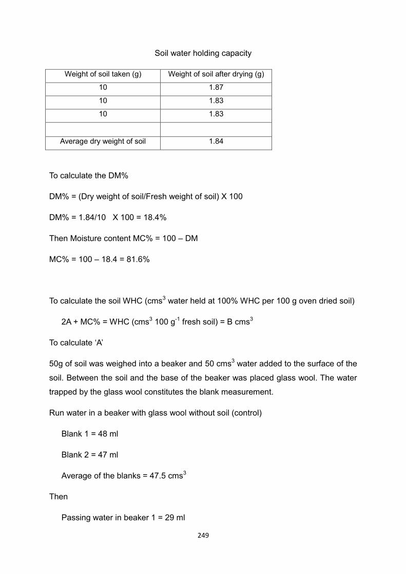
249
Soil water holding capacity
Weight of soil taken (g) Weight of soil after drying (g)
10 1.87
10 1.83
10 1.83
Average dry weight of soil 1.84
To calculate the DM%
DM% = (Dry weight of soil/Fresh weight of soil) X 100
DM% = 1.84/10 X 100 = 18.4%
Then Moisture content MC% = 100 – DM
MC% = 100 – 18.4 = 81.6%
To calculate the soil WHC (cms3 water held at 100% WHC per 100 g oven dried soil)
2A + MC% = WHC (cms3 100 g-1 fresh soil) = B cms3
To calculate ‘A’
50g of soil was weighed into a beaker and 50 cms3 water added to the surface of the
soil. Between the soil and the base of the beaker was placed glass wool. The water
trapped by the glass wool constitutes the blank measurement.
Run water in a beaker with glass wool without soil (control)
Blank 1 = 48 ml
Blank 2 = 47 ml
Average of the blanks = 47.5 cms3
Then
Passing water in beaker 1 = 29 ml

250
Passing water in beaker 2 = 23 ml
Passing water in beaker 3 = 25 ml
Average of run water = 25.7 ml
To calculate A
The volume of water retained by the soil was calculated from: 50 – (volume of
water retained by the glass wool + volume water collected) cms3
Water retained by soil ‘A’ = 50 – (2.5 ml + 25.7 ml) = 21.8 cms3
Where the volume of water retained by the glass wool (glass wool) = 50 ml – the
volume of water collected from the blank, which was: 50 – 47.5 = 2.5 cms3
Therefore: 2A + MC% = WHC (cms3 100 g-1 fresh soil) = B cms3
B ml = 2 (21.8) + 81.6 = 125.2 cms3
Then WHC = B cms3/ soil DM X 100 =
125.2/18.6 = 6.73 cms3 100 g of soil
125.2/18.6 X 100 = 673%
i.e 100 g of dry soil would contain 673 g of H2O
Total mass = 673 + 100 = 773 g
H2O % = 87.06% or 12.94 dry matter content.
Or
8706 cms3 per kg = 870%.
Dry weight and water holding capacity of spent brewery waste:
• Dry matter content (DM) spent grain:
Grain taken for each: 50 g
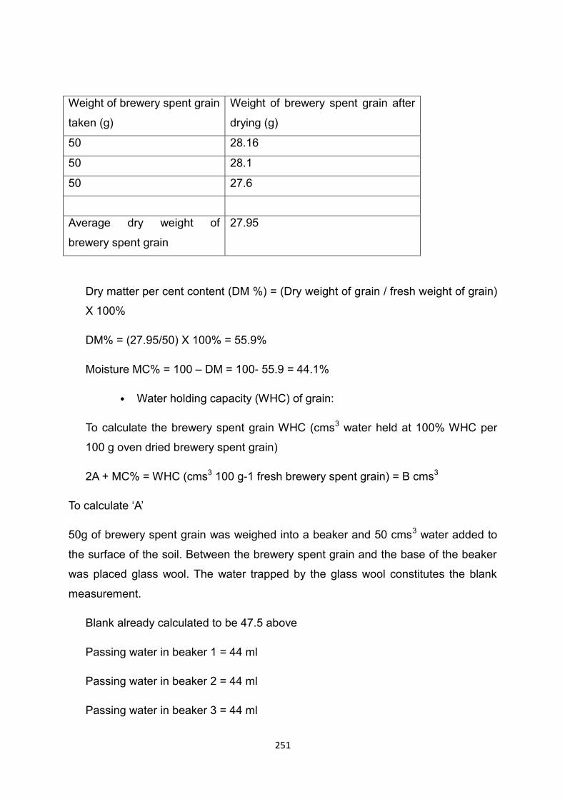
251
Weight of brewery spent grain
taken (g)
Weight of brewery spent grain after
drying (g)
50 28.16
50 28.1
50 27.6
Average dry weight of
brewery spent grain
27.95
Dry matter per cent content (DM %) = (Dry weight of grain / fresh weight of grain)
X 100%
DM% = (27.95/50) X 100% = 55.9%
Moisture MC% = 100 – DM = 100- 55.9 = 44.1%
• Water holding capacity (WHC) of grain:
To calculate the brewery spent grain WHC (cms3 water held at 100% WHC per
100 g oven dried brewery spent grain)
2A + MC% = WHC (cms3 100 g-1 fresh brewery spent grain) = B cms3
To calculate ‘A’
50g of brewery spent grain was weighed into a beaker and 50 cms3 water added to
the surface of the soil. Between the brewery spent grain and the base of the beaker
was placed glass wool. The water trapped by the glass wool constitutes the blank
measurement.
Blank already calculated to be 47.5 above
Passing water in beaker 1 = 44 ml
Passing water in beaker 2 = 44 ml
Passing water in beaker 3 = 44 ml

252
Average of run water = 44 ml
The volume of water retained by the grain was calculated from: 50 – (volume of
water retained by the muslin cloth + volume of water collected) cms3 = A which is
50 – (2.5 ml + 44 ml ) = 3.5 ml.
The volume of water retained by the glass wool = 50 ml – the volume of water
collected from the blanks = 50 – 47.25 = 2.5 cms3
To calculate grain WHC (cms3 water held at 100% WHC per 100 g oven dried
grain) 2A + MC% = WHC (ml 100 g-1 fresh grain) = B ml
B ml = 2 (3.5) + 44.1 = 51.1 cms3 Then
B ml / grain of DM X 100 = cms3 of water held by 100 g oven dried grain at 100%
WHC where
51.1/55.9 = 0.9141
WHC = 51.1/55.9 X 100 = 91.41%
i.e 100 g of dry brewery spent grain would contain 91.41 g of H2O
Total mass 91.41 + 100 = 191.41 g
H2O% = 47.76% or 52.24 dry matter content.
or
4776 cms3 per 1 kg of brewery spent grain or 478%

253
Appendix lll
Diesel used during tilling/turning of the soil during bioremediation with brewery
waste
Tilling the soil = 70 litre per day
First month tilling = 3 times
every month for 5 month = 2 times
The litres for first month = 210
The litres for 5 month = 700
The total litres for bioremediation with brewery waste = 910
Diesel used during tilling/turning of the soil during bioremediation without brewery
waste
Tilling the soil = 70 litre per day
First month tilling = 3 times
every month for 8 month = 2 times
The litres for first month = 210
The litres for 8 month = 1,120
The total litres for bioremediation without brewery waste = 1,330
Table 6.1: showing Calculation of litre of diesel used during tilling/turning of the soil during
bioremediation with brewery waste and without brewery spent grain.
Appendix lV
Conceptual Site RISK ASSESSMENT
TASK
Remediation of diesel contaminated site in Sunderland (case study site) for six
different remediation methods including natural attenuation, landfill disposal option,
soil vapour extraction, thermal desorption and bioremediation with and without
brewery spent grain
PRINCIPAL HAZARDS
Risk could arise due to the following hazards

254
• Collision with moving vehicles used during remediation activities.
• Migration of the pollutants to nearby water course and underground
water during remediation work- water contamination
• Emissions from hazardous waste such diesel from the soil – air
pollution.
• Risk of damaging underground pipe or utility services as a result of
excavating the soil or installing machines into the ground.
• Risk of dealing with volatile compounds
• Risk of environmental activist stopping the work or community
disturbance
PERSONS AT RISK AND ENVIRONMENTAL RISK
• Workers on site
• General public
• Ground water
• Surface water
• Air pollution
SIGNIFICANT RISKS
• Injuries due to collision with moving vehicles during remediation
• Air pollution due to release of CO2 and other air pollutants.
• Risk due contaminants migration to surface and underground water.
• Damage to underground pipes and utilities
• Risk of explosions of volatile compounds- diesel

255
CONSEQUENCES
• Serious water pollution, which is harmful to human, animal and water
life.
• Vehicle accidents could result to serious injury and death
• Hazardous chemical such as diesel which is carcinogenic
CONTROL MEASURES ( for remediation methods if there are available)
• Trenches are dug around the contaminated site to collect leaching
during bioremediation with and without brewery spent grain.
• Collected leaching is treated and monitor all time
• For soil vapour extraction and thermal desorption preventive measured
are in place to avoid underground water contamination by using state
of the heart technology. In addition nitrogen is added to capture gases
to prevent risk of explosion (during treatment and off-gas facility).
• Permission will be seek from local authority to closed the designated
site and road sign are put on site to warn of any danger especially from
heavy good vehicles.
• Air samples from thermal facility and soil vapour off-gas treatment plant
are checked to make sure meet regulatory requirement.

256
Appendix V
Electronic resources (internet)
URL-1 Soil phosphatase hand out (online) Available from:
http://www.envsci.rutgers.edu/~phelps/handout.pdf.
(Accessed on 29/09/2009)
URL-2 Introduction to waste hierarchy (online) Available from:
http://www.theengineer.co.uk/assets/getasset.aspx?liAssetID=25331.
(Accessed on 12/09/2009.)
URL-3 Waste strategy for England (WSFE) (2007) Available from:
: www.defra.gov.uk (Accessed on 05/10/2010).
URL-4 Formulation of R2A agar (online) Available from:
http://www.bd.com/ds/technicalCentre/inserts/R2A_agar_Davis.pdf
(Accessed on 10/08/2009)
URL-5 Formulation of Minimal agar (online) Available from:
http://www.bd.com/ds/technicalCentre/inserts/Minimal_agar_Davis.pdf
(Accessed on 10/08/2009)
URL-6: 17 Centers for Disease Control and Prevention. Toxicological Profile for Fuel
Oils. Available from: http://www.atsdr.cdc.gov/toxprofiles/tp75-c3.pdf (Last accessed:
08 December 2012)
URL- 7:
http://www.mpcd.info/index.php?option=com_content&view=article&id=443&Itemid=1
77
URL-8: EPA: overview of greenhouse gas: Methane emissions (Available:

257
http://epa.gov/climatechange/ghgemissions/gases/ch4.html)