interpreting regression results - college of...

Interpreting Regression Results

Although we classify the fitting procedure into different categories (such as linear fitting, nonlinear fitting), methods of interpreting the regression results are similar. For example, we can tell how good the fit is from R-square, reduced Chi-square value, diagnose the fitting result by residual analysis, etc. We will briefly explain how to interpret the regression result below.

Illustration of the Least-Squares Method

The most common method used to estimate the parameter values is the "least-squares method." The least-squares method minimizes the sum of the squares of the deviations of the theoretical data points from the experimental ones. This sum is the residual sum of squares and is computed as

The best-fit curve minimizes RSS. This figure illustrates the concept of least-squares fitting to a simple linear model (Note that multiple regression and nonlinear fitting are similar).

Topics covered in this section:

Illustration of the Least-Squares Method

Goodness of Fit

Confidence and Prediction Bands

Covariance and Correlation

Ellipse Plots

Significance of Parameters

Graphic Residual Analysis

The Fitting Process–Convergence, Tolerance and Dependencies

Model Diagnosis Using Dependency Values

Reference

of 18Interpreting Regression Results

1/15/2012file:///C:/Users/bknowlton/AppData/Local/Temp/~hh2A4C.htm

The Best-Fit Curve represents the assumed theoretical model. For a particular point (xi, yi) in the original

dataset, the corresponding theoretical value at xi is denoted by .

If there are two independent variables in the regression model, the least square estimation will minimize the deviation of experimental data points to the best fitted surface. When there are more then 3 independent variables, the fitted model will be a hypersurface. In this case, the fitted surface (or curve) will not be plotted when regression is performed.

Goodness of Fit

How good is the fit? One obvious metric is how close the fitted curve is from the actual data points. From the previous topic, we know that the residual sum of square (RSS) or the reduced chi-square value is a quantitative value that can be used to evaluate this kind of distance. However the value of residual sum of square (RSS) varies from dataset to dataset, making it necessary to rescale this value to a uniform range. On the other hand, one may want to use the mean of y value to describe the data feature. If it is the case, the fitted curve is a horizontal line, and the predictor x, cannot linearly predict the y value. To verify this, we first calculate the variation between data points and the mean, the "total sum of squares" about the mean, by

In least-squares fitting, the TSS can be divided into two parts: the variation explained by regression and that not explained by regression:

Clearly, the closer the data points are to the fitted curve, the smaller the RSS and the greater the proportion of the total variation that is represented by the SSreg. Thus, the ratio of SSreg to TSS can be used as one

The regression sum of squares, SSreg, is that portion of the variation that is explained by the regression model.The residual sum of squares, RSS, is that portion that is not explained by the regression model.



measure of the quality of the regression model. This quantity -- termed the coefficient of determination -- is computed as:

From the above equation, we can see that when using a good fitting model, R2 should vary between 0 and 1. A value close to 1 indicates that the fit is a good one.

Mathematically speaking, the degrees of freedom will affect R2. That is, when adding variables in the model, R2 will rise, but this does not imply a better fit. To avoid this effect, we can look at the adjusted R2:

From the equation, we can see that adjusted R2 overcomes the rise in R2, especially when fitting a small sample size (n) by multiple predictor (k) model. Though we usually term the coefficient of determination as "R-square", it is actually not a "square" value of R. For most cases, it is a value between 0 and 1, but you may also find negative R^2 when the fit is poor. This occurs because the equation to calculate R2 is R2 = 1 − RSS / TSS. The second term will be larger then 1, when a bad model is used.

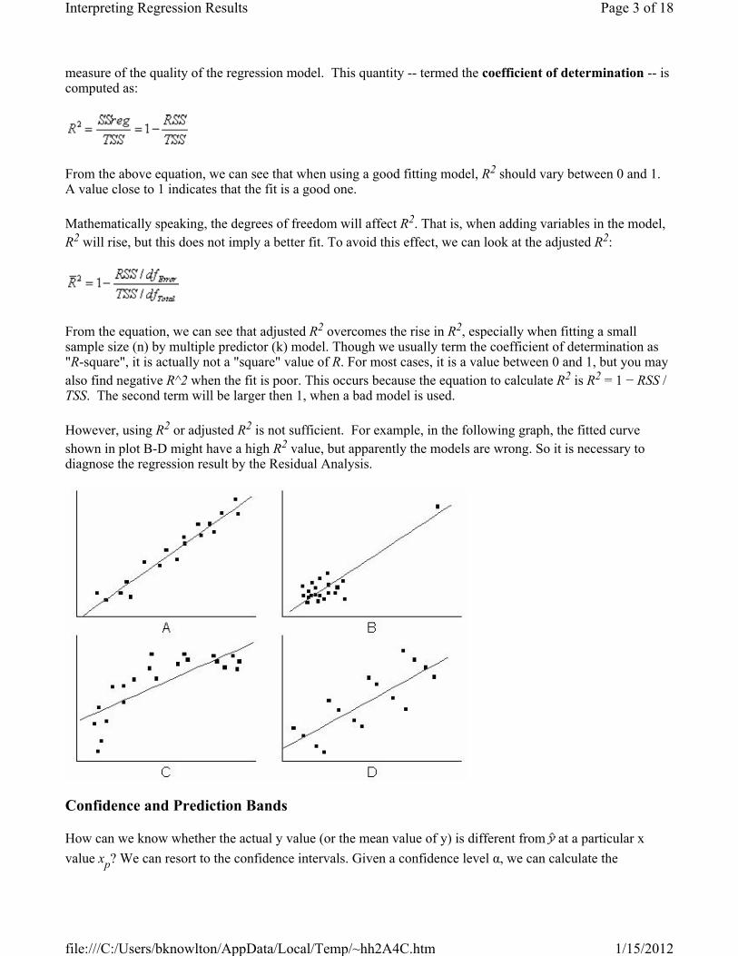
However, using R2 or adjusted R2 is not sufficient. For example, in the following graph, the fitted curve shown in plot B-D might have a high R2 value, but apparently the models are wrong. So it is necessary to diagnose the regression result by the Residual Analysis.

Confidence and Prediction Bands

How can we know whether the actual y value (or the mean value of y) is different from at a particular x value xp? We can resort to the confidence intervals. Given a confidence level α, we can calculate the



confidence interval for by:

In the following figure, for a chosen confidence level (95% by default), the confidence bands show the limits of all possible fitted lines for the given data. In other words, we have 95% confidence to say that the best-fit line (possibly one of the dash lines in the figure below) lies within the confidence bands.

From the expression of confidence interval, we know that the width of the confidence band is proportional to the standard error of predicted y value, sε. So the band will become narrower as the standard error decreases; if the error is zero, the confidence band will "collapse" into one single line. Besides, the term can

also affect the band width. The further xp is from , the greater becomes. Therefore, the confidence bands usually flare outward near the ends of the data range.

The case of prediction band is similar, but it uses a different expression:

It is different from the expression of confidence interval in that there is a constant term. Thus, the prediction band is wider than the confidence band.

The prediction band for the desired confidence level (1−α) is the interval within which 100(1−α)% of all the experimental points in a series of repeated measurements are expected to fall. By default, α is equal to 0.05. For a prediction band with (1−α)=0.95, we have 95% confidence to say that an expected data point will fall within this interval. In other words, if we add one more experiment data point whose independent variable is within the independent variable range of the original dataset, there is 95% chance that the data point will



appear within the prediction band.

Covariance and Correlation

The covariance value indicates the correlation between two variables, and the matrices of covariance in regression show the inter-correlations among all parameters. The diagonal values for covariance matrix is equal to the square of parameter error.

The correlation matrix rescales the covariance values so that their range is from -1 to +1. A value close to +1 means the two parameters are positively correlated, while a value close to -1 indicates negative correlation. And a zero value indicates that the two parameters are totally independent.

Ellipse Plots

We can use ellipse plots to graphically examine correlation in simple linear fitting. During linear regression, the two variables, X and Y are assumed to follow the bivariate normal distribution. This distribution is the co-effect of (X, Y) and is shaped like a bell surface.

For a given confidence level, such as 95%, we can conclude that 95% of variables pairs (x, y) will fall in the confidence area included by the upper ellipse, and the projection of the confidence area on XY plane is the confidence ellipse for prediction. The confidence ellipse for the population mean use the same idea and just shows the confidence ellipse of the mean ( , ).

The shape of the ellipse is determined by the correlation coefficient, r. Strong correlation means a long a(major semiaxis) and a short b (minor semiaxis). Also, the orientation of the ellipse also depends on r.

Significance of Parameters

Is every term in the regression model significant? Or does every predictor contribute to the response? The t-tests for coefficients answer these kinds of questions. The null hypothesis for a parameter's t-test is that this parameter is equal to zero. So if the null hypothesis is not rejected, the corresponding predictor will be viewed as insignificant, which means that it has little to do with the response.

The t-test can also be used as a detection tool. For example, in polynomial regression, we can use it to determine the proper order of the polynomial model. We add higher order terms until a t-test for the newly-



added term suggests that it is insignificant.

Graphic Residual Analysis

The residual is defined as:

Residual plots can be used to assess the quality of a regression. Currently, five types of residual plots are supported by the linear fitting dialog box:

Residual vs. Independent

Residual vs. Predicted Value

Residual vs. Order of the Data

Histogram of the Residual

Residual Lag Plot

These residual plots can be used to assess the quality of the regression. You can examine the underlying statistical assumptions about residuals such as constant variance, independence of variables and normality of the distribution. For these assumptions to hold true for a particular regression model, the residuals would have to be randomly distributed around zero.

Different types of residual plots can be used to check the validity of these assumptions and provide information on how to improve the model. For example, the scatter plot of the residuals will be disordered if the regression is good. The residuals should not show any trend. A trend would indicate that the residuals were not independent. On the other hand, a histogram plot of the residuals should exhibit a symmetric bell-shaped distribution, indicating that the normality assumption is likely to be true.

Checking the error variance

Checking the process drift

Checking independence of the error term

Checking normality of variance

Improving the regression model using residuals plots

Detecting outliers by transforming residuals

Residual contour plots for surface fitting

Checking the error variance

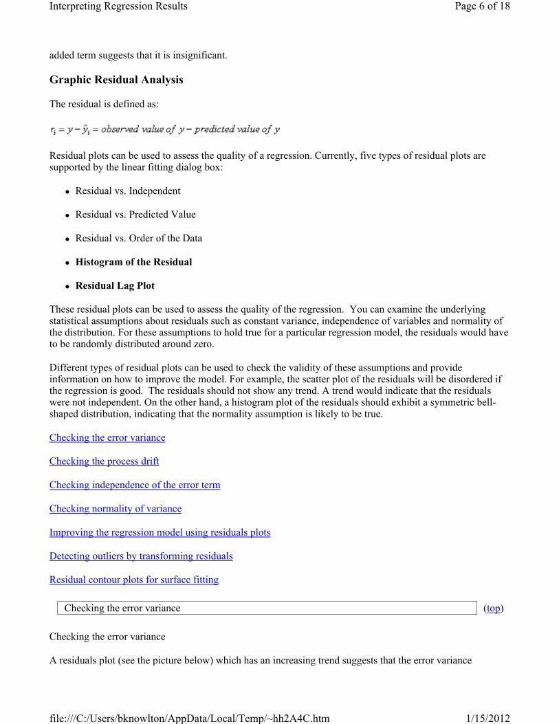
A residuals plot (see the picture below) which has an increasing trend suggests that the error variance

Checking the error variance (top)



increases with the independent variable; while a distribution that reveals a decreasing trend indicates that the error variance decreases with the independent variable. Neither of these distributions are constant variance patterns. Therefore they indicate that the assumption of constant variance is not likely to be true and the regression is not a good one. On the other hand, a horizontal-band pattern suggests that the variance of the residuals is constant.

Checking the process drift

The Residual vs. Order of the Data plot can be used to check the drift of the variance (see the picture below) during the experimental process, when data are time-ordered. If the residuals are randomly distributed around zero, it means that there is no drift in the process.

Checking the process drift (top)



Checking independence of the error term

The Residual Lag Plot (see the picture below), constructed by plotting residual (i) against residual (i-1), is useful for examining the dependency of the error terms. Any non-random pattern in a lag plot suggests that the variance is not random.

If the data being analyzed is time series data (data recorded sequentially), the Residual vs. Order of the Dataplot will reflect the correlation between the error term and time. Fluctuating patterns around zero will indicate

Checking independence of the error term (top)



that the error term is dependent.

Residual Lag Plot showing that the error term is independent.



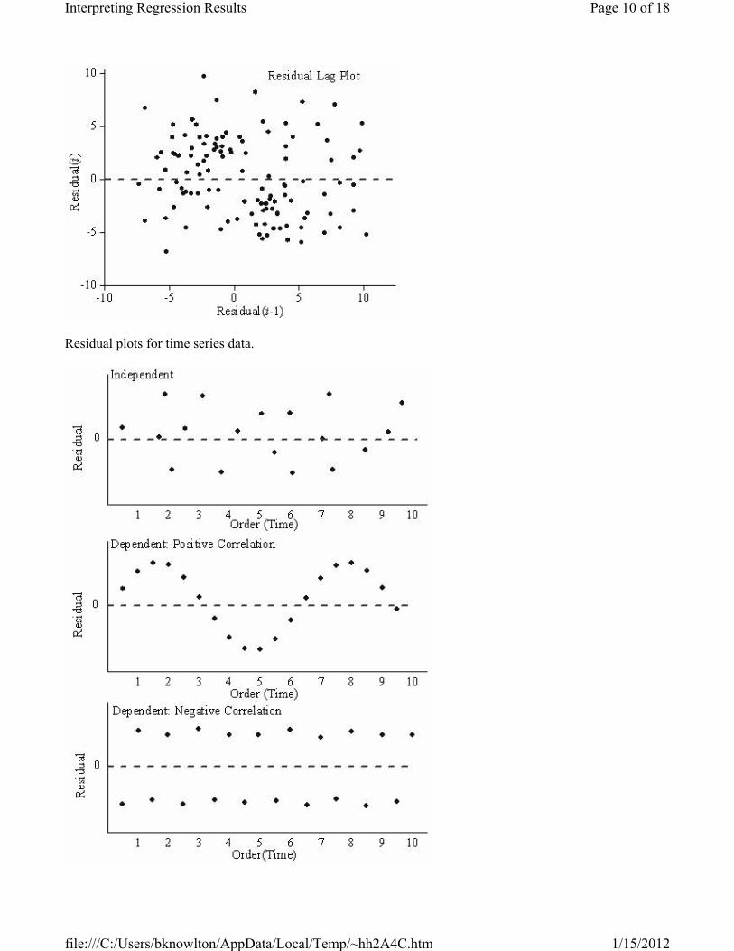
Residual plots for time series data.



Checking normality of variance

The Histogram of the Residual can be used to check whether the variance is normally distributed. A symmetric bell-shaped histogram which is evenly distributed around zero indicates that the normality assumption is likely to be true. If the histogram indicates that random error is not normally distributed, it suggests that the model's underlying assumptions may have been violated.

Histogram of the Residuals showing that the deviation is normally distributed.

Improving the regression model using residuals plots

The pattern structures of residual plots not only help to check the validity of a regression model, but they can also provide hints on how to improve it. For example , a curved pattern in the Residual vs. Independent plot suggests that a higher order term should be introduced to the fitting model.

Checking normality of variance (top)

Improving the regression model using residuals plots (top)



This is only one example and, certainly, there is much more that can be surmised from studying residual plot patterns. We suggest that you refer to the statistical references given at the end of this chapter/section, for more information.

Detecting outliers by transforming residuals

When looking for outliers in your data, it may be useful to transform the residuals to obtain standardized, studentized or studentized deleted residuals. These transformed residuals are computed as follows:

Standardized

Studentized

Studentized deleted

In the equations for the Studentized and Studentized deleted residuals, hi is the ith diagonal element of the matrix, P:

Detecting outliers by transforming residuals (top)



where F is the partial derivatives matrix for a nonlinear regression model.

In a linear regression model, the independent matrix, X, is simply equal to F:

As an example of the use of transformed residuals, standardized residuals rescale residual values by the regression standard error, so if the regression assumptions hold -- that is, the data are distributed normally --about 95% data points should fall within 2σ around the fitted curve. Consequently, 95% of the standardized residuals will fall between -2 and +2 in the residual plot.

These variations of residual plots are very useful in detecting outliers. For example, in the Standardized Residual vs. Independent Plots, the residuals are rescaled by the regression standard error. If the regression assumption holds, that is, the data is distributed normally, about 95% data points should be located within 2σ around the fitted curve, and consequently, 95% of the standardized residuals will fall between -2 and +2, as shown in the graph below.

So residuals out of this range should be more closely examined, because these points may be outliers.

Residual contour plots for surface fitting

When fitting a surface with an OriginPro built-in function, a contour plot of residuals in the XY plane is produced. Contour intervals are determined by the sigma value (the model error). As in the case of 2D fitting, a good fit of the regression surface should produce no recognizable patterns in the contour plot of the residuals.

The Fitting Process Convergence, Tolerance and Dependencies

Residual contour plots for surface fitting (top)



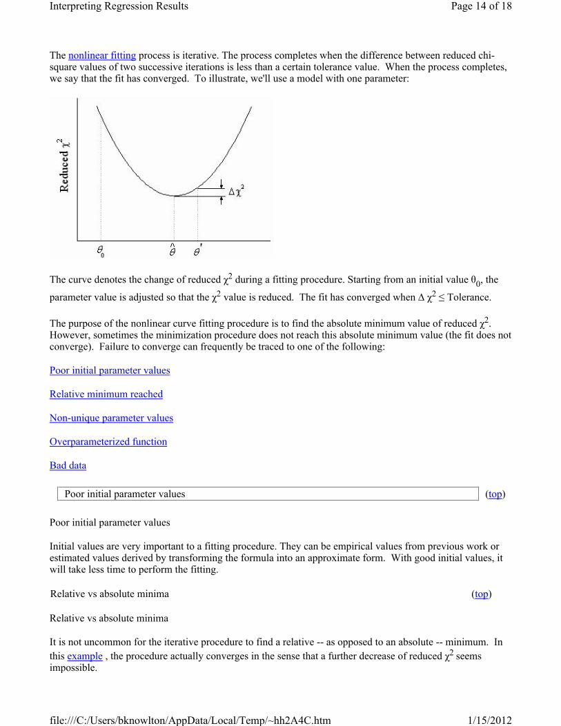
The nonlinear fitting process is iterative. The process completes when the difference between reduced chi-square values of two successive iterations is less than a certain tolerance value. When the process completes, we say that the fit has converged. To illustrate, we'll use a model with one parameter:

The curve denotes the change of reduced χ2 during a fitting procedure. Starting from an initial value θ0, the

parameter value is adjusted so that the χ2 value is reduced. The fit has converged when ∆ χ2 ≤ Tolerance.

The purpose of the nonlinear curve fitting procedure is to find the absolute minimum value of reduced χ2. However, sometimes the minimization procedure does not reach this absolute minimum value (the fit does not converge). Failure to converge can frequently be traced to one of the following:

Poor initial parameter values

Relative minimum reached

Non-unique parameter values

Overparameterized function

Bad data

Poor initial parameter values

Initial values are very important to a fitting procedure. They can be empirical values from previous work or estimated values derived by transforming the formula into an approximate form. With good initial values, it will take less time to perform the fitting.

Relative vs absolute minima

It is not uncommon for the iterative procedure to find a relative -- as opposed to an absolute -- minimum. In this example , the procedure actually converges in the sense that a further decrease of reduced χ2 seems impossible.

Poor initial parameter values (top)

Relative vs absolute minima (top)



The problem is that you do not even know if the routine has reached an absolute or a relative minimum. The only way to be certain that the iterative procedure is reaching an absolute minimum is to start fitting from several different initial parameter values and observe the results. If you repeatedly get the same final result, it is unlikely that a local minimum has been found.

Non-unique parameter values

The most common problem that arises in nonlinear fitting is that no matter how you choose the initial parameter values, the fit does not seem to converge. Some or all parameter values continue to change with successive iterations and they eventually diverge, producing arithmetic overflow or underflow. This should indicate that you need to do something about the fitting function and/or data you are using. There is simply no single set of parameter values which best fit your data.

Over-parameterized functions

If the function parameters have the same differential with respect to independent variables, it may suggest that the function is overparameterized. In such cases, the fitting procedure will not converge. For example in the following model

A is the amplitude and x0 is the horizontal offset. However, you can rewrite the function as

In other words, if, during the fitting procedure, the values of A and x0 change so that the combination B

remains the same, the reduced χ2 value will not change . Any attempts to further improve the fit are not likely to be productive.

Non-unique parameter values (top)

Over-parameterized functions (top)



If you see one of the following, it indicates that something is wrong:

The parameter error is very large relative to the parameter value. For example, if the width of the Gaussian curve is 0.5 while the error is 10, the result for the width will be meaningless as the fit has not converged.

The parameter dependence (for one or more parameters) is very close to one. You should probably remove or fix the value of parameters whose dependency is close to one, since the fit does not seem to depend upon the parameter.

Note, however, that over-parameterization does not necessarily mean that the parameters in the model have no physical meanings. It may suggest that there are infinite solutions and you should apply constraints to the fit process.

Bad data

Even when the function is not theoretically overparameterized, the iterative procedure may behave as if it were, due to the fact that the data do not contain enough information for some or all of the parameters to be determined. This usually happens when the data are available only in a limited interval of the independent variable(s). For example, if you are fitting a non-monotonic function such as the Gaussian to monotonic data, the nonlinear fitter will experience difficulties in determining the peak center and peak width, since the data can describe only one flank of the Gaussian peak.

Model Diagnosis Using Dependency Values

We can also assess the quality of a fit model using the Dependency value. A value close to 1 indicates that the function may be (but is not necessarily) overparameterized and that the parameter may be redundant. You should include restrictions to make sure that the fitting model is meaningful. In this example, where sample data is fitted by the ExpDecay1 function:

Bad data (top)



You can see that the Dependency values for parameters x0 and A1 are large, which suggests that these two variables are highly dependent. In other words, one parameter varies with the other, without changing the R2

value. This means that the result may not valid. We can see from the graph that the X value starts from about 500. To compensate for this, we can perform the fitting by fixing x0 as 500 to generate a reasonable dependency result:

Moreover, dependent parameters may also lead to some meaningless results. For example, if we fit the same data by ExpDec1 model, the result may be as follows:



You can see that the parameter value A is too large and may not make sense. In this case, we should use bounds or constraints to limit the parameter values so that they fall within a reasonable range.

References

Bruce Bowerman, Richard T. O'Connell. 1997. Applied Statistics: Improving Business Processes. The McGraw-Hill Companies, Inc.

Sanford Weisberg. 2005. Applied Linear Regression. Third Edition. John Wiley & Son, Inc., Hoboken, New Jersey.

William H. Press et al. 2002. Numerical Recipes in C++, 2nd ed. Cambridge University Press: New York.

Marko Ledvij. Curve Fitting Made Easy. The Industrial Physicist. Apr./May 2003. 9:24-27.



interpreting regression results - college of...

Documents