interpreting and presenting statistical resultsweb.stanford.edu/~tomz/software/clarsc.pdf ·...
TRANSCRIPT
Interpreting and Presenting Statistical
Results
Mike Tomz Jason Wittenberg Harvard University
APSA Short Course September 1, 1999
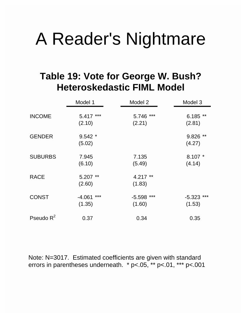
A Reader's Nightmare
Table 19: Vote for George W. Bush? Heteroskedastic FIML Model
Note: N=3017. Estimated coefficients are given with standard errors in parentheses underneath. * p<.05, ** p<.01, *** p<.001
INCOME 5.417 *** 5.746 *** 6.185 **(2.10) (2.21) (2.81)
GENDER 9.542 * 9.826 **(5.02) (4.27)
SUBURBS 7.945 7.135 8.107 *(6.10) (5.49) (4.14)
RACE 5.207 ** 4.217 **(2.60) (1.83)
CONST -4.061 *** -5.598 *** -5.323 ***(1.35) (1.60) (1.53)
Pseudo R2 0.37 0.34 0.35
Model 1 Model 2 Model 3
Our method helps researchers
• Convey results in a reader-friendly manner
• Uncover new facts about the political world
The method does not require
• collecting new
data
• changing the statistical model
• introducing new
assumptions
This course has three parts.
1. The problem 2. A solution 3. Examples, with
software
Good methods of interpretation should satisfy three criteria:
1. Convey numerically precise
estimates of the quantities of substantive interest
2. Include reasonable estimates of uncertainty about those estimates
3. Require no specialized knowledge to understand
The most common methods of interpretation do not satisfy our criteria.
1. Listing coefficients and se's
• not intrinsically interesting • hard to understand
1. Computing expected values or first differences exclusively
• ignores sampling error and fundamental uncertainty
Best current practice
• “Fitted”, “predicted” (expected)
values
Compute an expected value of the dependent variable given the estimated coefficients and interesting values of the explanatory variables.
• First Differences
Compute the difference between two expected values.
Both ignore sampling error and fundamental uncertainty.
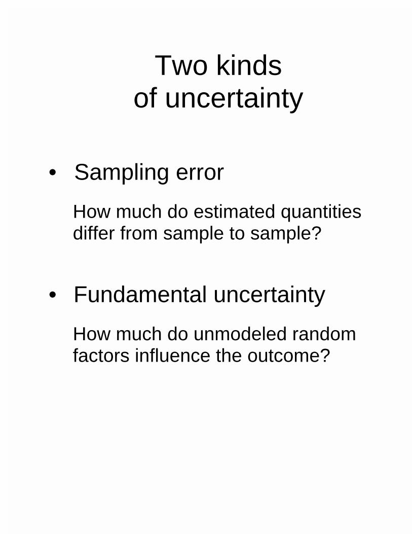
Two kinds of uncertainty
• Sampling error
How much do estimated quantities differ from sample to sample?
• Fundamental uncertainty
How much do unmodeled random factors influence the outcome?
A better method
Our Goal
To obtain precise quantities of interest and estimates of uncertainty that are easy to understand.
The technique
Use simulation to extract all available information from a statistical model.
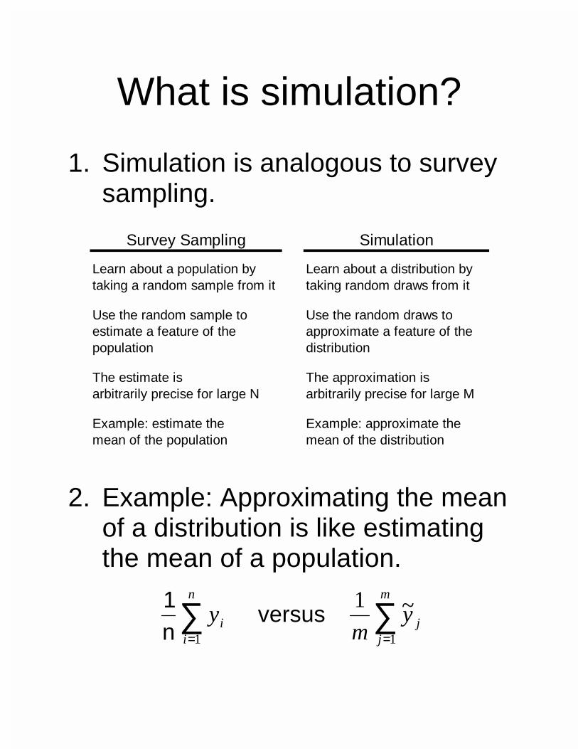
What is simulation?
1. Simulation is analogous to survey sampling.
Survey Sampling Simulation
Learn about a population by taking a random sample from it
Learn about a distribution by taking random draws from it
Use the random sample to estimate a feature of the population
Use the random draws to approximate a feature of the distribution
The estimate is arbitrarily precise for large N
The approximation is arbitrarily precise for large M
Example: estimate the mean of the population
Example: approximate the mean of the distribution
2. Example: Approximating the mean of a distribution is like estimating the mean of a population.
∑∑==
m
jj
n
ii y
my
11
~1 versus
n1
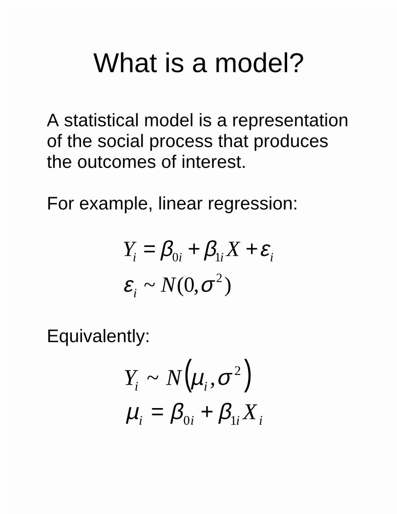
What is a model? A statistical model is a representation of the social process that produces the outcomes of interest. For example, linear regression:
),0(~ 2
10
σεεββ
N
XY
i
iiii ++=
Equivalently:
( )iiii
ii
X
NY
10
2,~
ββµσµ
+=
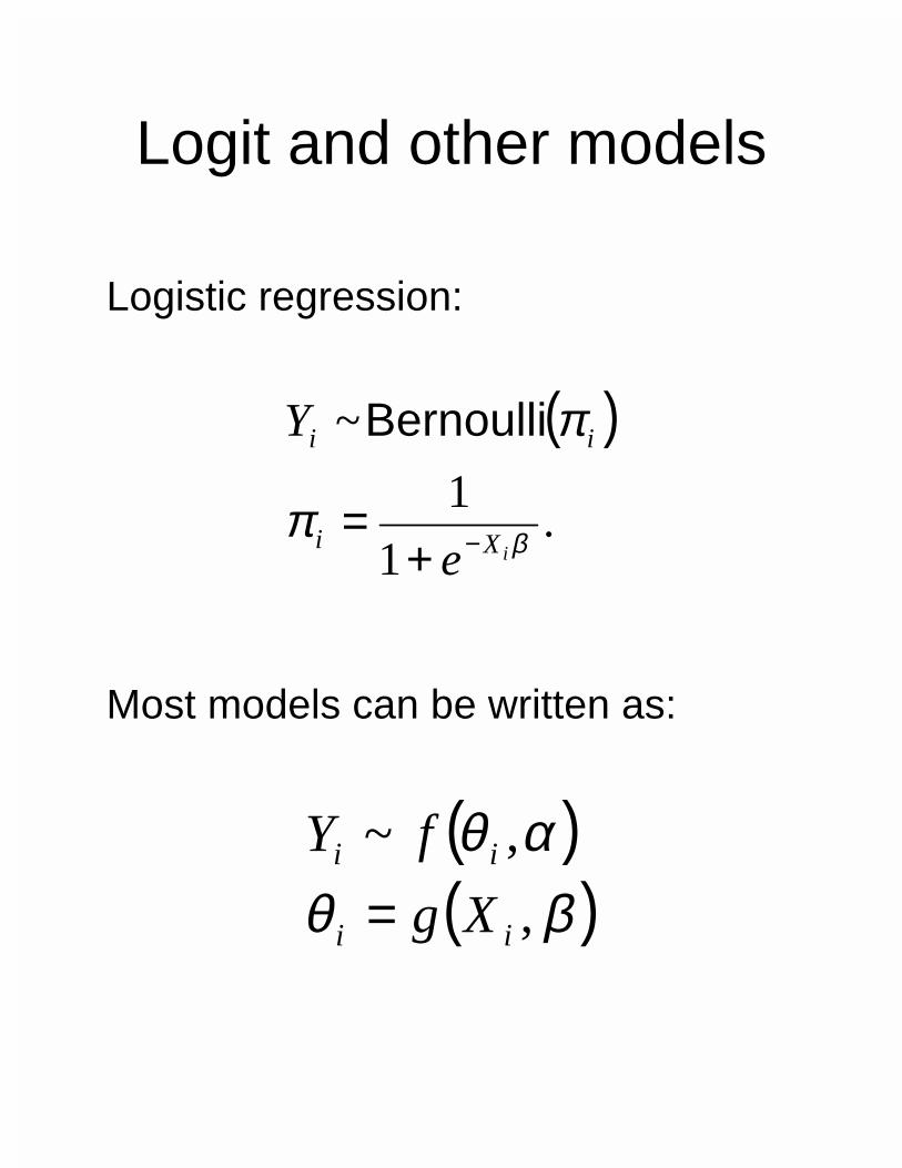
Logit and other models Logistic regression:
( )
.1
1
~
βπ
π
iXi
ii
e
Y
−+=
Bernoulli
Most models can be written as:
( )( )βθ
αθ,
,~
ii
ii
Xg
fY
=
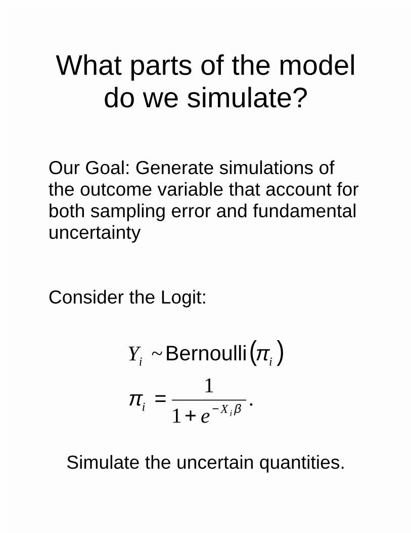
What parts of the model do we simulate?
Our Goal: Generate simulations of the outcome variable that account for both sampling error and fundamental uncertainty Consider the Logit:
( )
.1
1
~
βπ
π
iXi
ii
e
Y
−+=
Bernoulli
Simulate the uncertain quantities.
How do we simulate the parameters?
1. Obtain the estimated
coefficients and variance matrix
2. Draw (simulate) the
parameters from a multivariate normal distribution
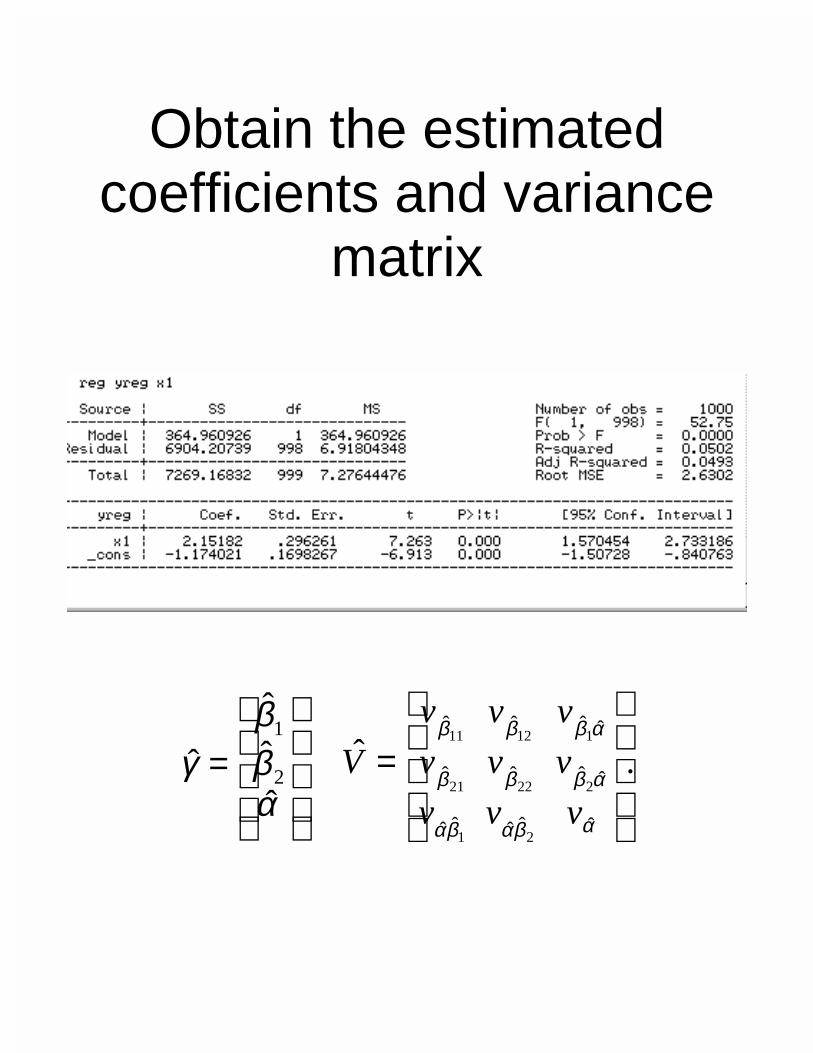
Obtain the estimated coefficients and variance
matrix
=
αββ
γˆ
ˆˆ
ˆ 2
1
.ˆ
ˆˆˆˆˆ
ˆˆˆˆ
ˆˆˆˆ
21
22221
11211
=
αβαβα
αβββ
αβββ
vvv
vvv
vvv
V
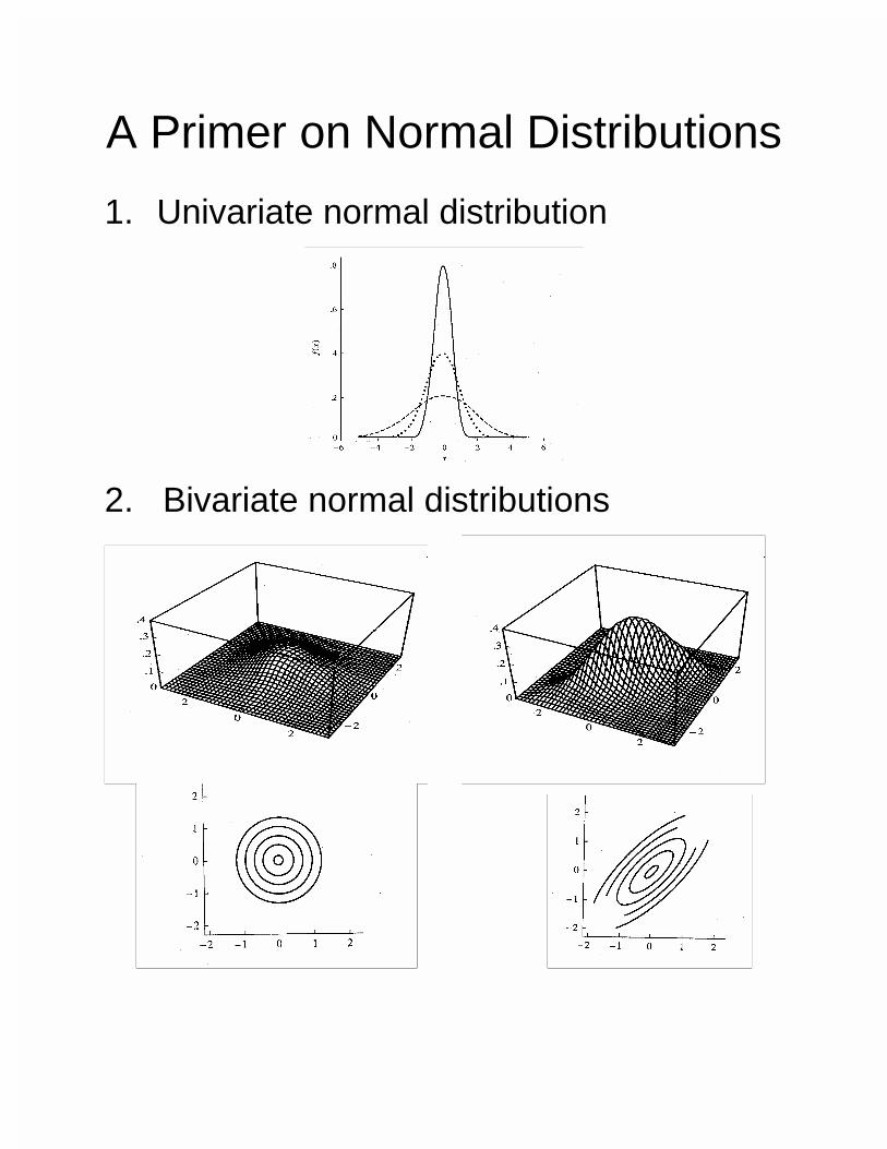
A Primer on Normal Distributions
1. Univariate normal distribution
2. Bivariate normal distributions
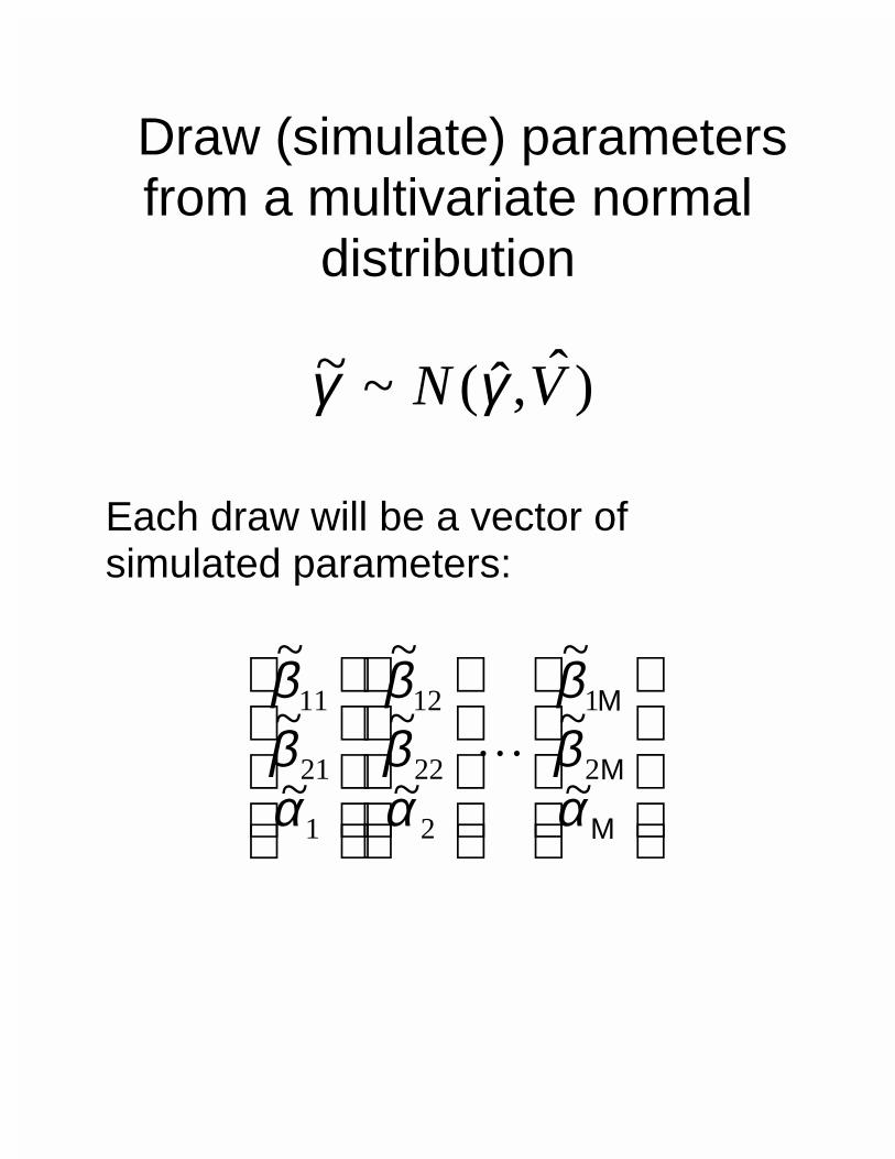
Draw (simulate) parameters from a multivariate normal
distribution
)ˆ,ˆ(~~ VN γγ
Each draw will be a vector of simulated parameters:
M
M
M
αββ
αββ
αββ
~
~~
~
~~
~
~~
2
1
2
22
12
1
21
11
�
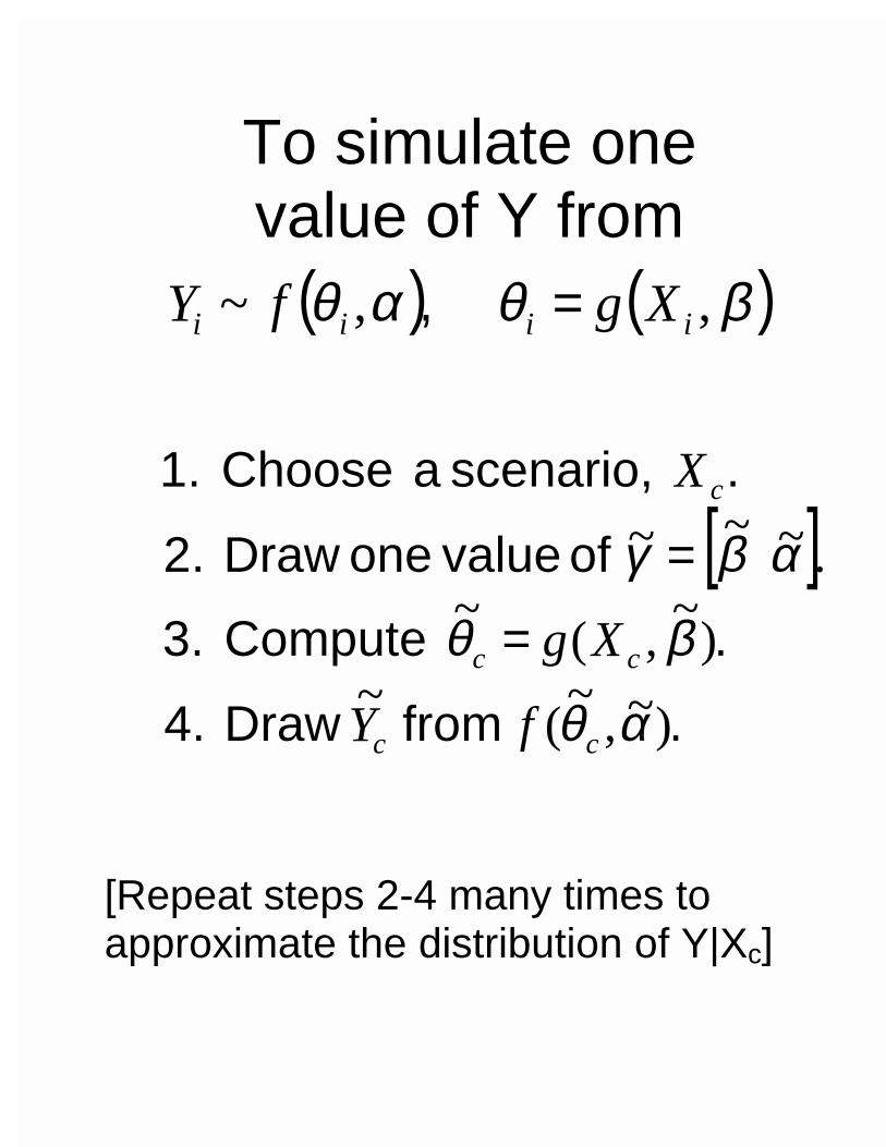
To simulate one value of Y from
( ) ( )βθαθ ,,~ iiii XgfY = ,
[ ]
. from Draw 4.
. Compute 3.
of value oneDraw 2.
. scenario, a Choose 1.
)~,~
(~
)~
,(~
.~~~
αθ
βθ
αβγ
cc
cc
c
fY
Xg
X
=
=
[Repeat steps 2-4 many times to approximate the distribution of Y|Xc]
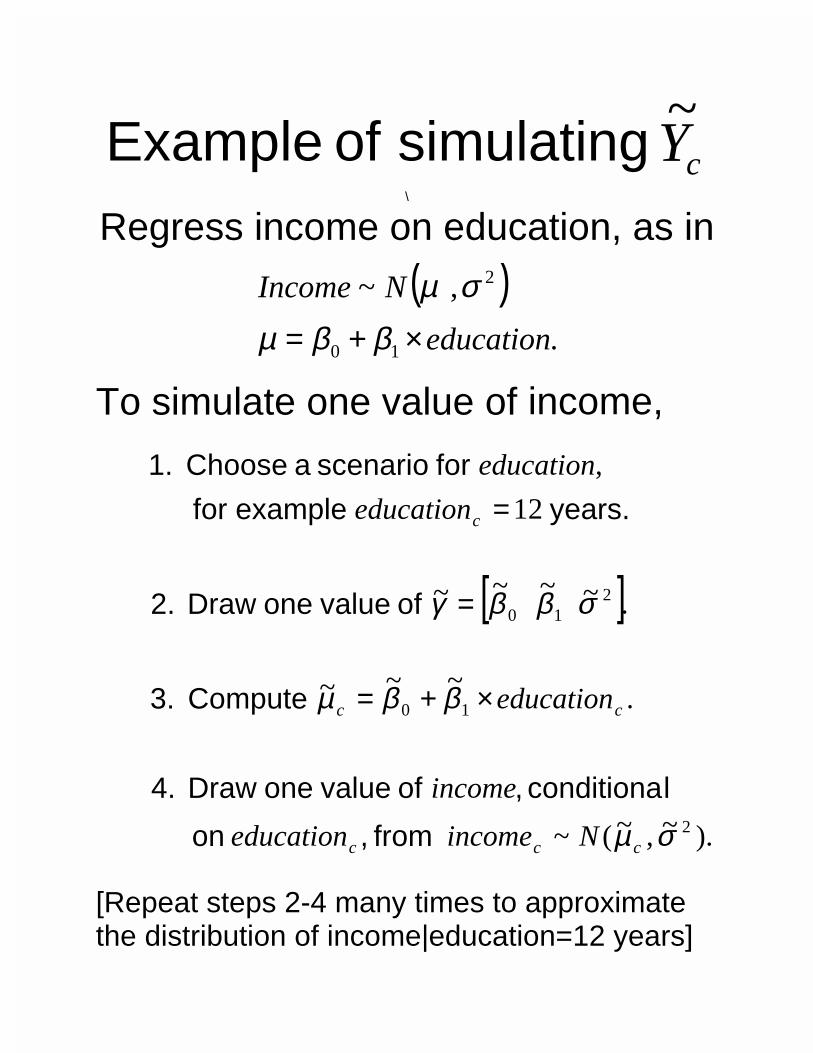
cY~
simulating of Example \
Regress income on education, as in
( ).
,~
10
2
education
NIncome
×+= ββµσµ
To simulate one value of income,
[ ]
).~,~(~
.~~~
.~~~~
12
,
2
10
210
σµ
ββµ
σββγ
ccc
cc
c
Nincomeeducation
income
education
education
education
from , on
lconditiona , of value oneDraw 4.
Compute 3.
of value oneDraw 2.
years. example for
for scenario a Choose 1.
×+=
=
=
[Repeat steps 2-4 many times to approximate the distribution of income|education=12 years]
:including quantity,any
compute can we With cY~
• Predicted values • Expected values
• First differences
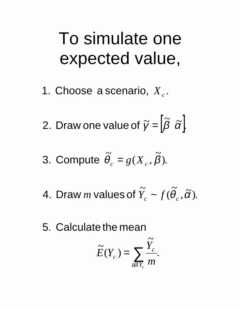
To simulate one expected value,
[ ]
.~
)(~
)~,~
(~
)~
,(~
.~~~
~∑=
=
=
cY
cc
cc
cc
c
m
YYE
fYm
Xg
X
all
mean the Calculate 5.
. ~ of values Draw 4.
. Compute 3.
of value oneDraw 2.
. scenario, a Choose 1.
αθ
βθ
αβγ
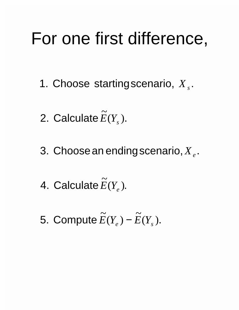
For one first difference,
).(~
)(~
)(~
.
).(~
se
e
e
s
s
YEYE
YE
X
YE
X
− Compute 5.
. Calculate 4.
scenario, ending an Choose 3.
Calculate 2.
. scenario, starting Choose 1.
With many draws of the quantity of interest, we
can calculate:
• Average values • Confidence intervals
• Anything else we want!
Tricks for simulating parameters
1. Simulate betas and
ancillary parameters. 2. Transform parameters to
make them unbounded and symmetric.
Tricks for simulating the quantity of interest
1. Increase simulations for
more precision, reduce for computational speed.
2. Reverse transformations
of the dependent variable. 3. Advanced users can take
shortcuts to simulate the expected value and other quantities.
The method in practice (Please try this at home!)
There are three main steps.
1. Estimate the model and simulate the parameters.
2. Choose a scenario for the explanatory variables.
3. Simulate quantities of interest.
We provide software to get you started.
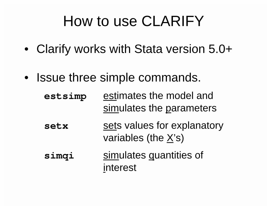
How to use CLARIFY • Clarify works with Stata version 5.0+ • Issue three simple commands.
estsimp estimates the model and simulates the parameters
setx sets values for explanatory variables (the X’s)
simqi simulates quantities of interest
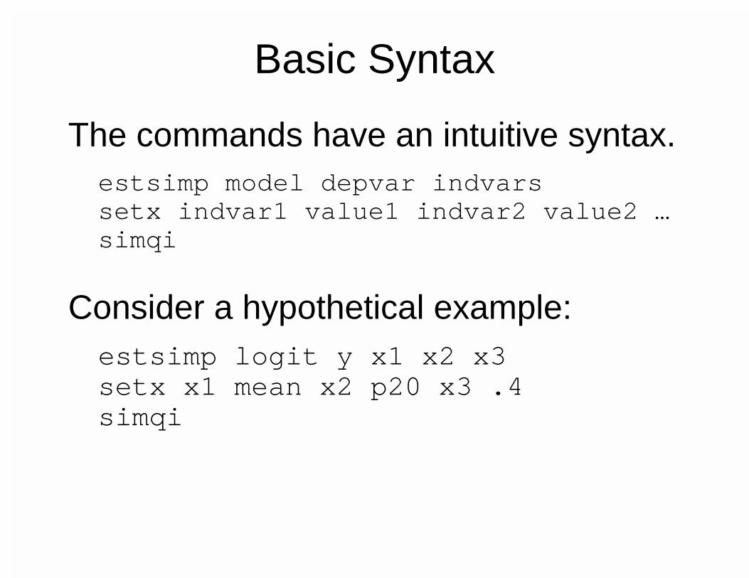
Basic Syntax
The commands have an intuitive syntax.
estsimp model depvar indvars setx indvar1 value1 indvar2 value2 … simqi
Consider a hypothetical example:
estsimp logit y x1 x2 x3 setx x1 mean x2 p20 x3 .4 simqi
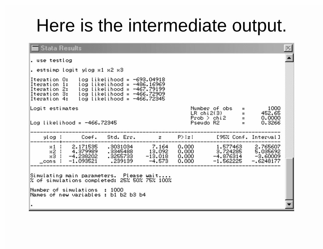
Here is the intermediate output.
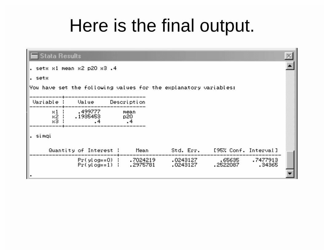
Here is the final output.
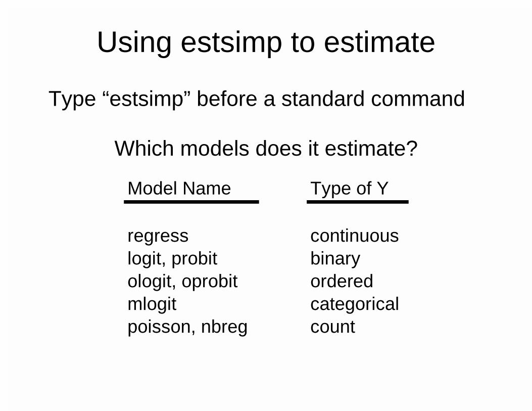
Using estsimp to estimate Type “estsimp” before a standard command
Which models does it estimate?
Model Name Type of Y
regress continuouslogit, probit binaryologit, oprobit orderedmlogit categoricalpoisson, nbreg count
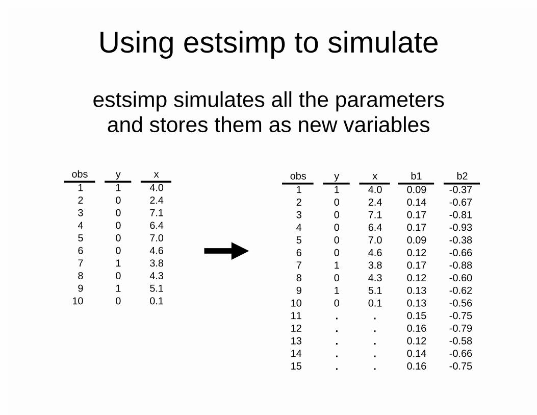
Using estsimp to simulate
estsimp simulates all the parameters
and stores them as new variables
y1 1 4.0 0.09 -0.372 0 2.4 0.14 -0.673 0 7.1 0.17 -0.814 0 6.4 0.17 -0.935 0 7.0 0.09 -0.386 0 4.6 0.12 -0.667 1 3.8 0.17 -0.888 0 4.3 0.12 -0.609 1 5.1 0.13 -0.62
10 0 0.1 0.13 -0.5611 . 0.15 -0.7512 . 0.16 -0.7913 . 0.12 -0.5814 . 0.14 -0.6615 . 0.16 -0.75
.
.
.
obs x b1 b2
.
.
y1 1 4.02 0 2.43 0 7.14 0 6.45 0 7.06 0 4.67 1 3.88 0 4.39 1 5.1
10 0 0.1
obs x
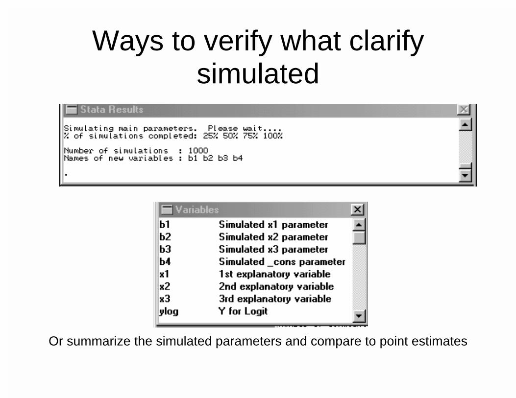
Ways to verify what clarify simulated
Or summarize the simulated parameters and compare to point estimates
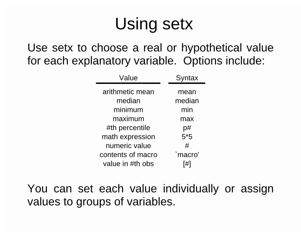
Using setx
Use setx to choose a real or hypothetical value for each explanatory variable. Options include:
You can set each value individually or assign values to groups of variables.
Value Syntax
arithmetic mean meanmedian median
minimum minmaximum max
#th percentile p#math expression 5*5numeric value #
contents of macro `macro'value in #th obs [#]
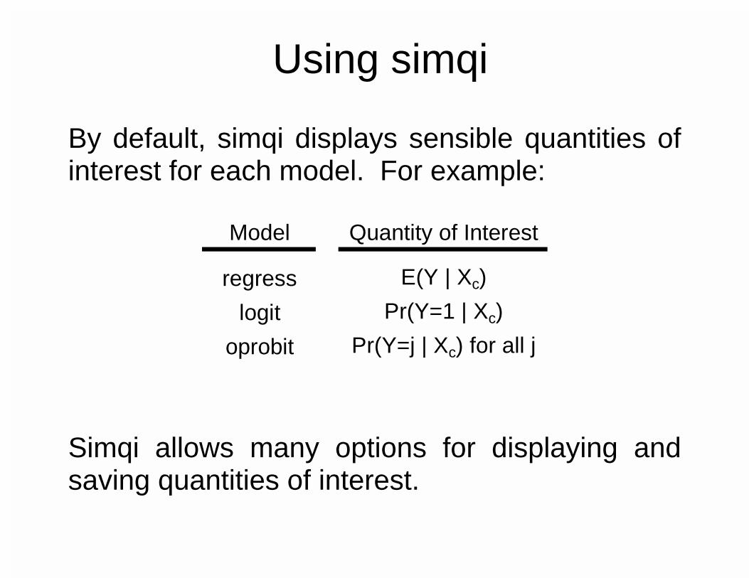
Using simqi
By default, simqi displays sensible quantities of interest for each model. For example:
Simqi allows many options for displaying and saving quantities of interest.
Model Quantity of Interest
regress E(Y | Xc)
logit Pr(Y=1 | Xc)
oprobit Pr(Y=j | Xc) for all j
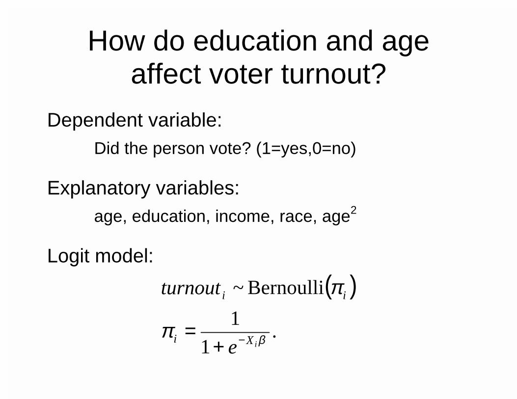
How do education and age affect voter turnout?
Dependent variable:
Did the person vote? (1=yes,0=no)
Explanatory variables:
age, education, income, race, age2
Logit model:
( )
.1
1
Bernoulli~
βπ
π
iXi
ii
e
turnout
−+=
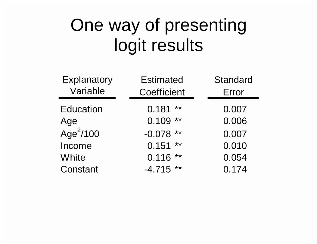
One way of presenting logit results
ExplanatoryVariable
Education 0.181 ** 0.007Age 0.109 ** 0.006Age2/100 -0.078 ** 0.007Income 0.151 ** 0.010White 0.116 ** 0.054Constant -4.715 ** 0.174
StandardError
EstimatedCoefficient
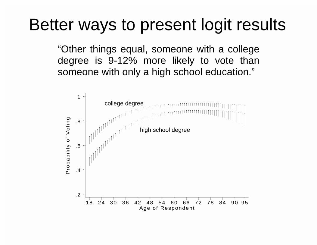
Better ways to present logit results
“Other things equal, someone with a college degree is 9-12% more likely to vote than someone with only a high school education.”
Pro
ba
bil
ity
of
Vo
tin
g
Age of Respondent18 24 30 36 42 48 54 60 66 72 78 84 90 95
.2
.4
.6
.8
1college degree
high school degree
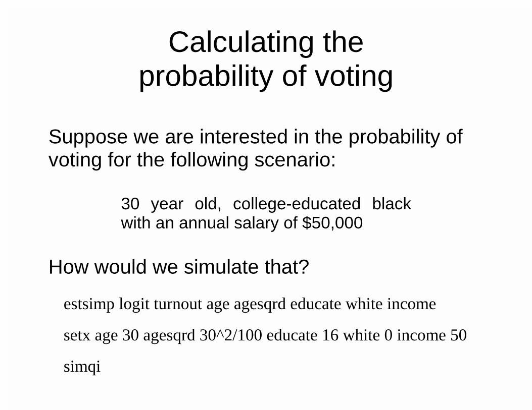
Calculating the probability of voting
Suppose we are interested in the probability of voting for the following scenario:
30 year old, college-educated black with an annual salary of $50,000
How would we simulate that?
estsimp logit turnout age agesqrd educate white income
setx age 30 agesqrd 30^2/100 educate 16 white 0 income 50
simqi
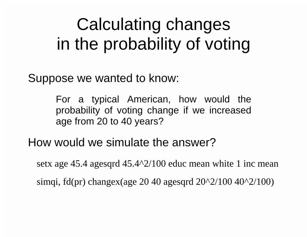
Calculating changes in the probability of voting
Suppose we wanted to know:
For a typical American, how would the probability of voting change if we increased age from 20 to 40 years?
How would we simulate the answer?
setx age 45.4 agesqrd 45.4^2/100 educ mean white 1 inc mean
simqi, fd(pr) changex(age 20 40 agesqrd 20^2/100 40^2/100)
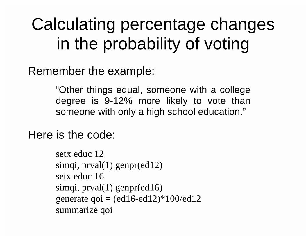
Calculating percentage changes in the probability of voting
Remember the example:
“Other things equal, someone with a college degree is 9-12% more likely to vote than someone with only a high school education.”
Here is the code:
setx educ 12 simqi, prval(1) genpr(ed12) setx educ 16 simqi, prval(1) genpr(ed16) generate qoi = (ed16-ed12)*100/ed12 summarize qoi
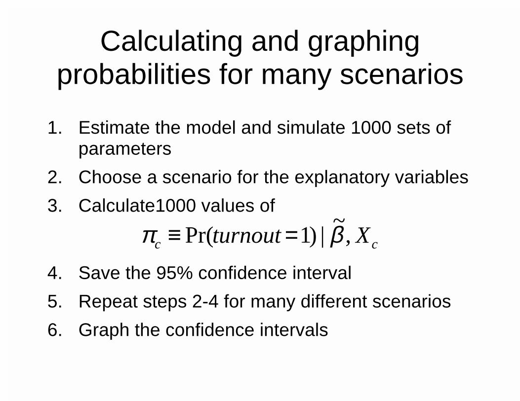
Calculating and graphing probabilities for many scenarios
1. Estimate the model and simulate 1000 sets of
parameters
2. Choose a scenario for the explanatory variables
3. Calculate1000 values of
cc Xturnout ,~
|)1Pr( βπ =≡
4. Save the 95% confidence interval
5. Repeat steps 2-4 for many different scenarios
6. Graph the confidence intervals
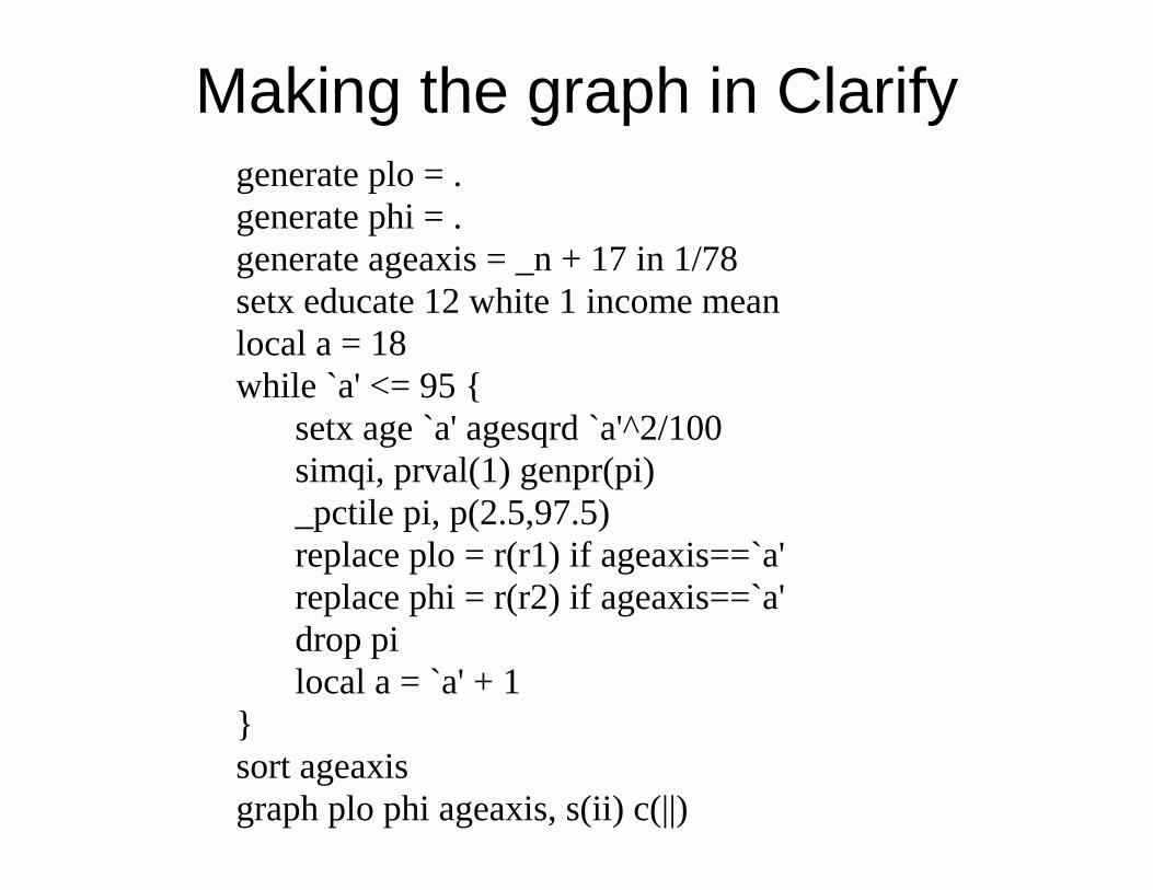
Making the graph in Clarify
generate plo = . generate phi = . generate ageaxis = _n + 17 in 1/78 setx educate 12 white 1 income mean local a = 18 while `a' <= 95 { setx age `a' agesqrd `a'^2/100 simqi, prval(1) genpr(pi) _pctile pi, p(2.5,97.5) replace plo = r(r1) if ageaxis==`a' replace phi = r(r2) if ageaxis==`a' drop pi local a = `a' + 1 } sort ageaxis graph plo phi ageaxis, s(ii) c(||)
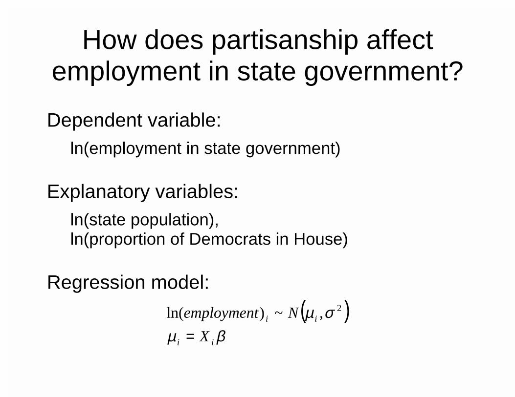
How does partisanship affect employment in state government? Dependent variable:
ln(employment in state government) Explanatory variables:
ln(state population), ln(proportion of Democrats in House)
Regression model:
( )βµ
σµ
ii
ii
X
Nemployment
=
2,~)ln(
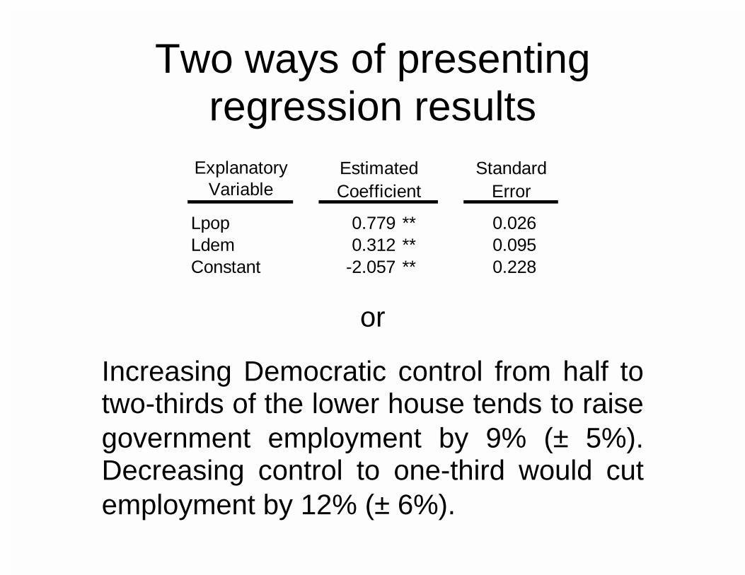
Two ways of presenting regression results
Explanatory
Variable
Lpop 0.779 ** 0.026Ldem 0.312 ** 0.095Constant -2.057 ** 0.228
Estimated StandardCoefficient Error
or
Increasing Democratic control from half to two-thirds of the lower house tends to raise government employment by 9% (± 5%). Decreasing control to one-third would cut employment by 12% (± 6%).
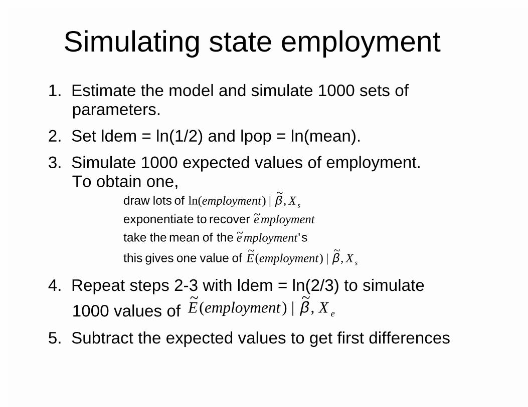
Simulating state employment
1. Estimate the model and simulate 1000 sets of parameters.
2. Set ldem = ln(1/2) and lpop = ln(mean).
3. Simulate 1000 expected values of employment. To obtain one,
s
s
XemploymentE
mploymente
mploymente
Xemployment
,~
|)(~
~
~,
~|)ln(
β
β
of value one gives this
s' the of mean the take
recover to teexponentia
of lotsdraw
4. Repeat steps 2-3 with ldem = ln(2/3) to simulate
1000 values of eXemploymentE ,~
|)(~ β
5. Subtract the expected values to get first differences
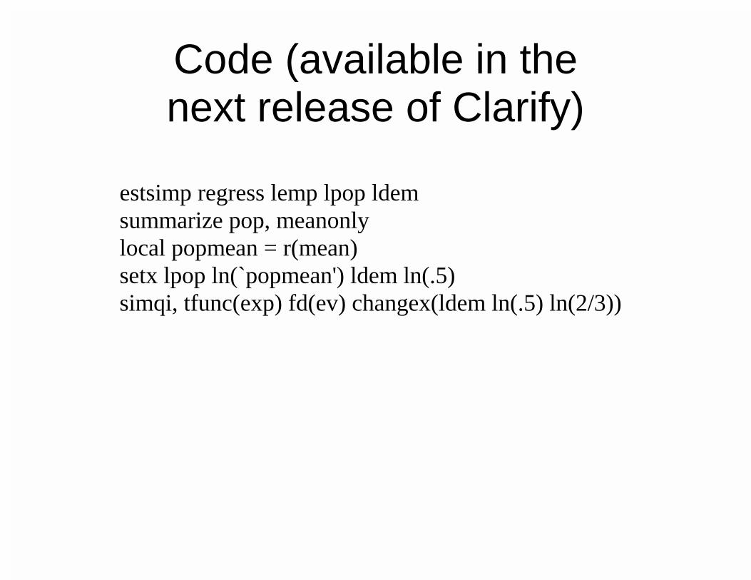
Code (available in the next release of Clarify)
estsimp regress lemp lpop ldem summarize pop, meanonly local popmean = r(mean) setx lpop ln(`popmean') ldem ln(.5) simqi, tfunc(exp) fd(ev) changex(ldem ln(.5) ln(2/3))
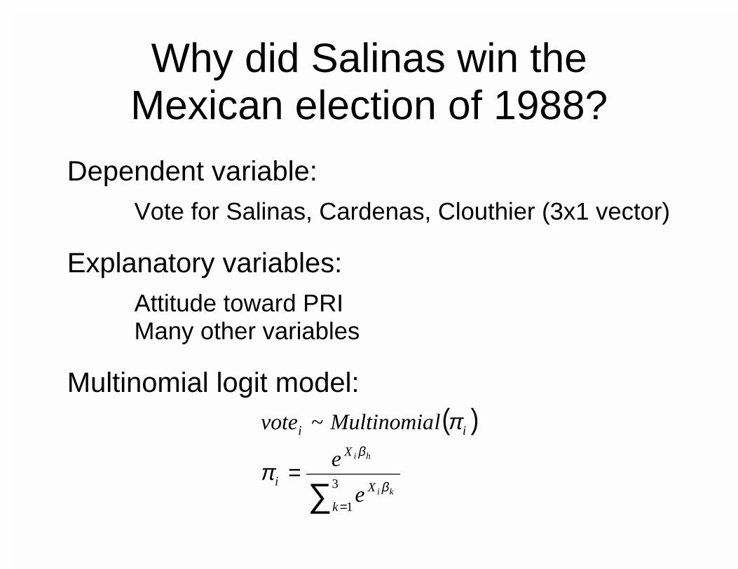
Why did Salinas win the Mexican election of 1988?
Dependent variable:
Vote for Salinas, Cardenas, Clouthier (3x1 vector)
Explanatory variables:
Attitude toward PRI Many other variables
Multinomial logit model:
( )
∑ =
=3
1
~
k
X
X
i
ii
ki
hi
e
e
lMultinomiavote
β
β
π
π
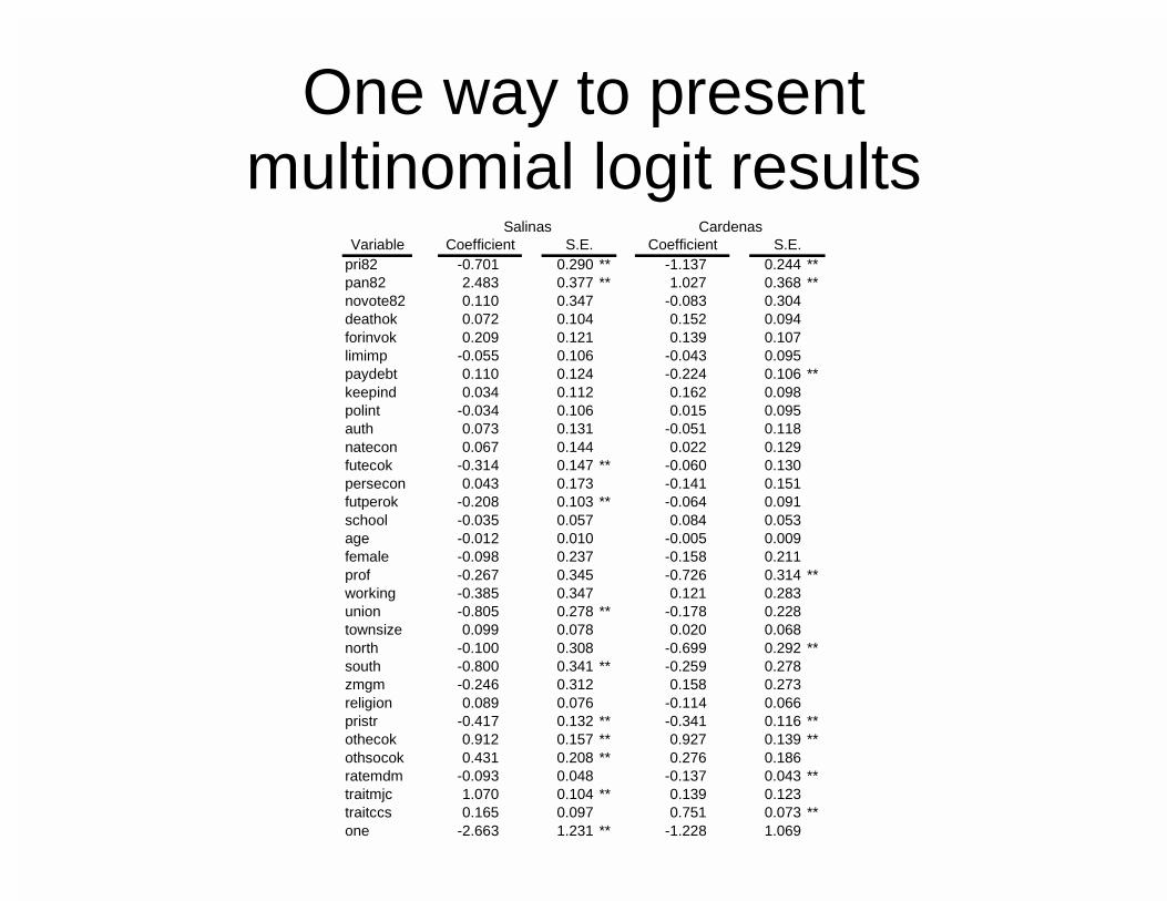
One way to present multinomial logit results
Variablepri82 -0.701 0.290 ** -1.137 0.244 **pan82 2.483 0.377 ** 1.027 0.368 **novote82 0.110 0.347 -0.083 0.304deathok 0.072 0.104 0.152 0.094forinvok 0.209 0.121 0.139 0.107limimp -0.055 0.106 -0.043 0.095paydebt 0.110 0.124 -0.224 0.106 **keepind 0.034 0.112 0.162 0.098polint -0.034 0.106 0.015 0.095auth 0.073 0.131 -0.051 0.118natecon 0.067 0.144 0.022 0.129futecok -0.314 0.147 ** -0.060 0.130persecon 0.043 0.173 -0.141 0.151futperok -0.208 0.103 ** -0.064 0.091school -0.035 0.057 0.084 0.053age -0.012 0.010 -0.005 0.009female -0.098 0.237 -0.158 0.211prof -0.267 0.345 -0.726 0.314 **working -0.385 0.347 0.121 0.283union -0.805 0.278 ** -0.178 0.228townsize 0.099 0.078 0.020 0.068north -0.100 0.308 -0.699 0.292 **south -0.800 0.341 ** -0.259 0.278zmgm -0.246 0.312 0.158 0.273religion 0.089 0.076 -0.114 0.066pristr -0.417 0.132 ** -0.341 0.116 **othecok 0.912 0.157 ** 0.927 0.139 **othsocok 0.431 0.208 ** 0.276 0.186ratemdm -0.093 0.048 -0.137 0.043 **traitmjc 1.070 0.104 ** 0.139 0.123traitccs 0.165 0.097 0.751 0.073 **one -2.663 1.231 ** -1.228 1.069
Coefficient S.E. S.E.CoefficientCardenasSalinas
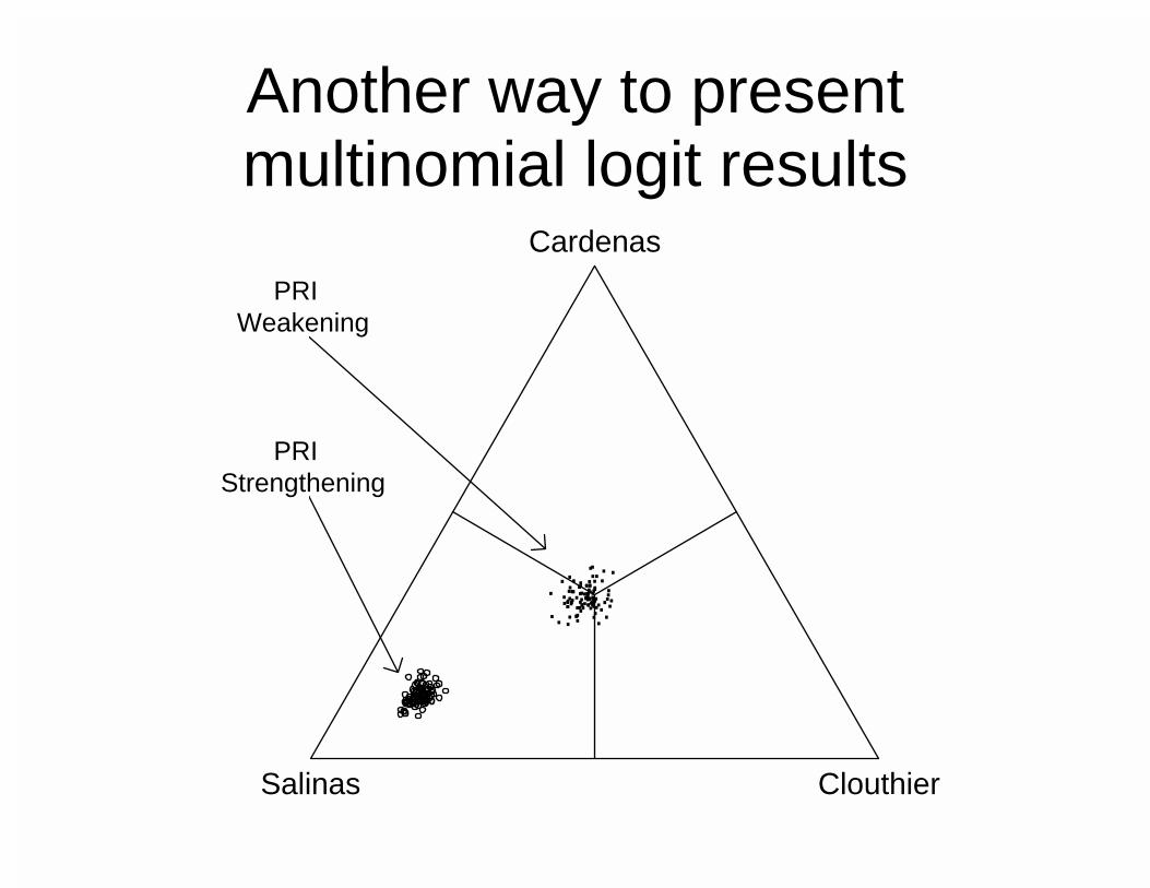
Another way to present multinomial logit results
Cardenas
ClouthierSalinas
.. ... .....
. ... ...
. .... ... ...... .
......
..
...
...... .....
. ..... ....
.. .....
... ....
..... .... ... .... .
. ... .
PRI Weakening
PRI Strengthening
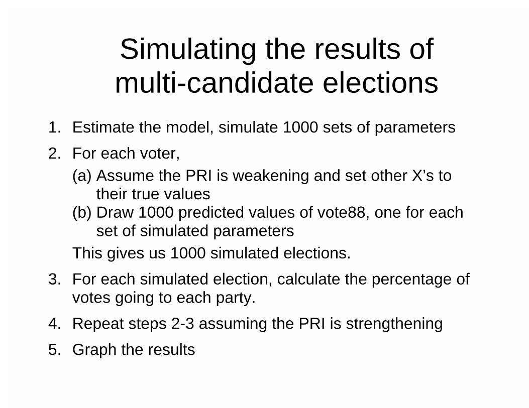
Simulating the results of multi-candidate elections
1. Estimate the model, simulate 1000 sets of parameters
2. For each voter,
(a) Assume the PRI is weakening and set other X’s to their true values
(b) Draw 1000 predicted values of vote88, one for each set of simulated parameters
This gives us 1000 simulated elections.
3. For each simulated election, calculate the percentage of votes going to each party.
4. Repeat steps 2-3 assuming the PRI is strengthening
5. Graph the results
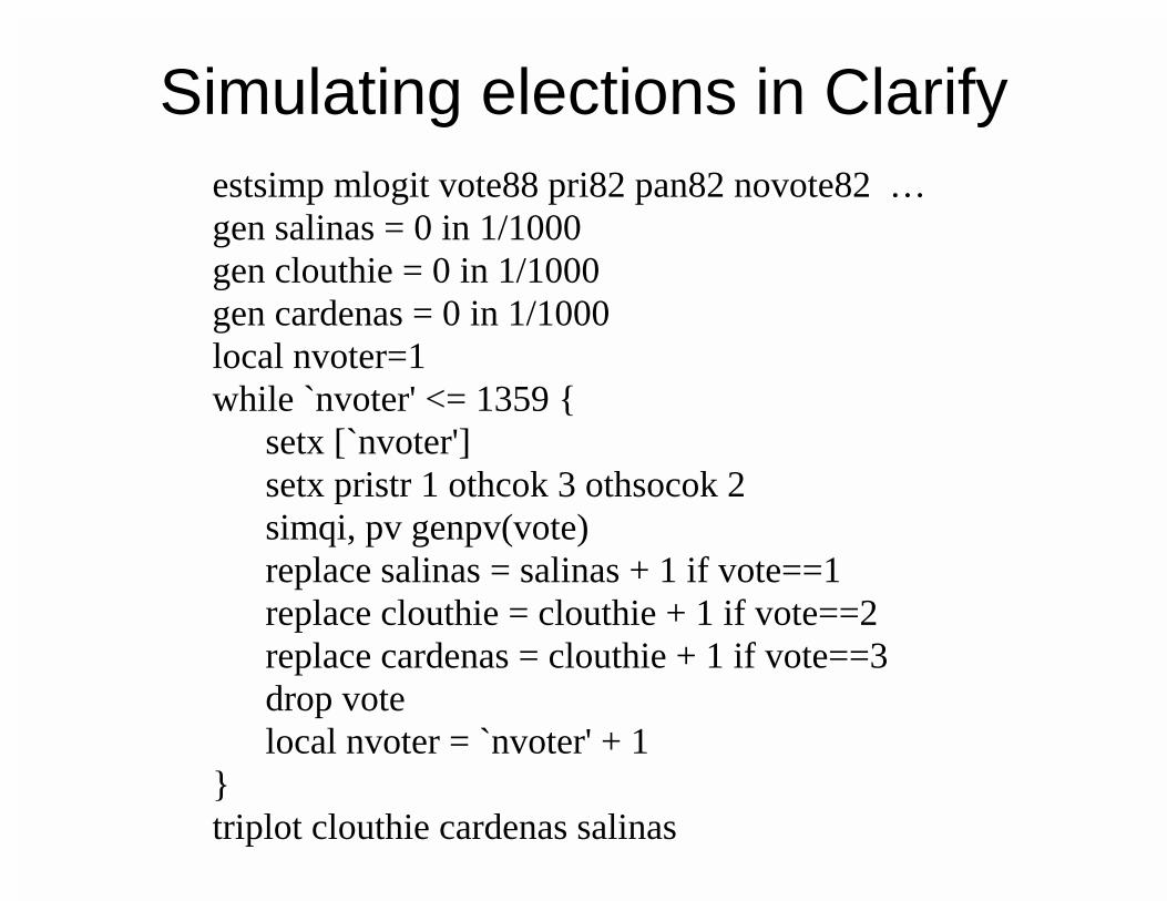
Simulating elections in Clarify
estsimp mlogit vote88 pri82 pan82 novote82 … gen salinas = 0 in 1/1000 gen clouthie = 0 in 1/1000 gen cardenas = 0 in 1/1000 local nvoter=1 while `nvoter' <= 1359 { setx [`nvoter'] setx pristr 1 othcok 3 othsocok 2 simqi, pv genpv(vote) replace salinas = salinas + 1 if vote==1 replace clouthie = clouthie + 1 if vote==2 replace cardenas = clouthie + 1 if vote==3 drop vote local nvoter = `nvoter' + 1 } triplot clouthie cardenas salinas
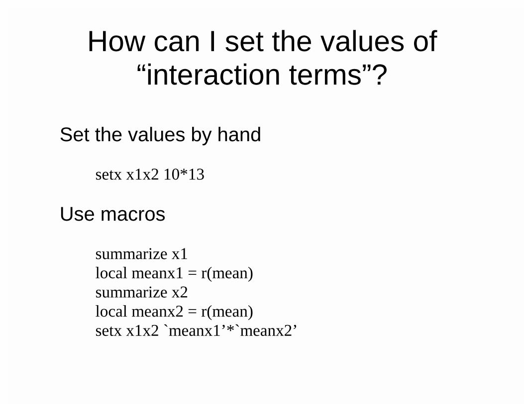
How can I set the values of “interaction terms”?
Set the values by hand
setx x1x2 10*13 Use macros
summarize x1 local meanx1 = r(mean) summarize x2 local meanx2 = r(mean) setx x1x2 `meanx1’*`meanx2’
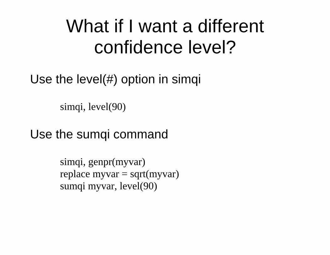
What if I want a different confidence level?
Use the level(#) option in simqi
simqi, level(90) Use the sumqi command
simqi, genpr(myvar) replace myvar = sqrt(myvar) sumqi myvar, level(90)
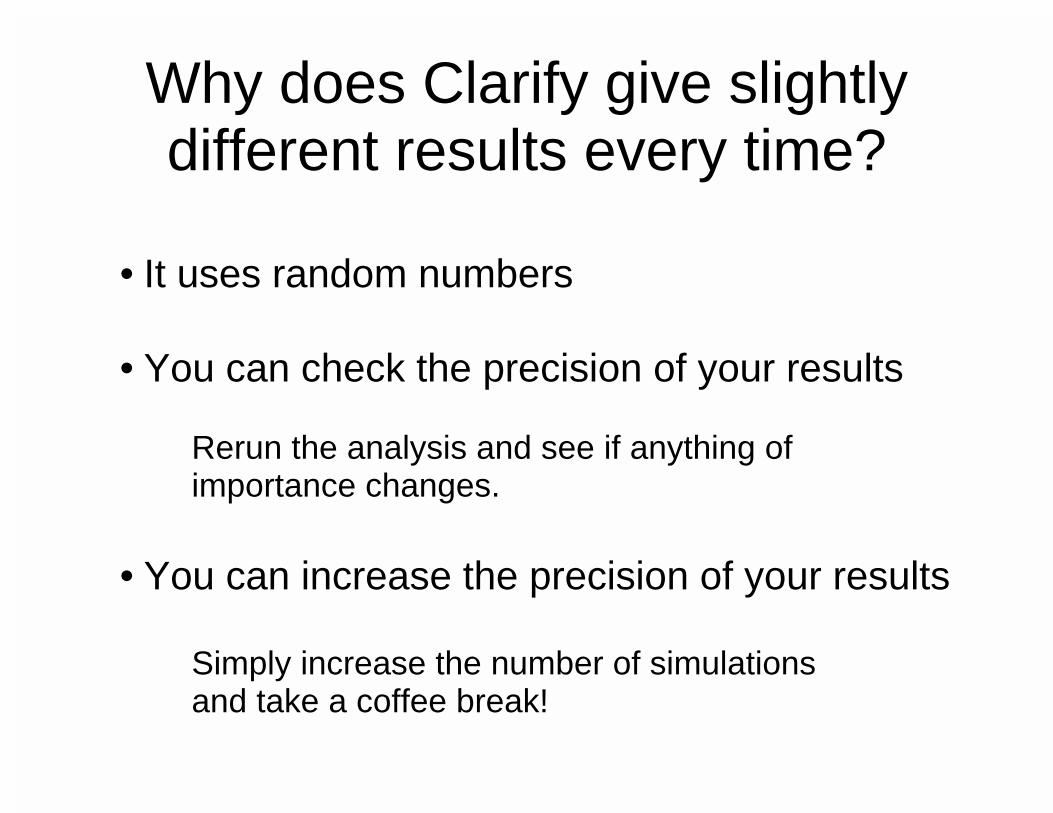
Why does Clarify give slightly different results every time?
• It uses random numbers
• You can check the precision of your results
Rerun the analysis and see if anything of importance changes.
• You can increase the precision of your results
Simply increase the number of simulations and take a coffee break!