interpreting and presenting regression resultsinterpreting and presenting regression results...
TRANSCRIPT
Interpreting and Presenting Regression Results
Frederick J. Boehmke
Department of Political ScienceUniversity of Iowa
Prepared for presentation at the University of Kentucky.
February 29, 2008
Boehmke Interactions Workshop February 29, 2008 1 / 40
Introduction
Setup of interaction hypotheses.
Boehmke Interactions Workshop February 29, 2008 2 / 40
Introduction
Setup of interaction hypotheses.
Discussion of common claims.
Boehmke Interactions Workshop February 29, 2008 2 / 40
Introduction
Setup of interaction hypotheses.
Discussion of common claims.
Implementing tests.
Boehmke Interactions Workshop February 29, 2008 2 / 40
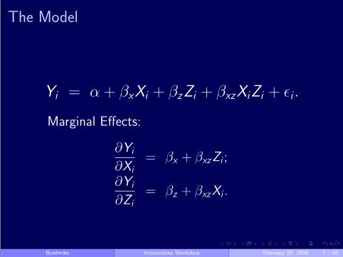
The Model
Yi = α + βxXi + βzZi + βxzXiZi + εi .
Marginal Effects:
∂Yi
∂Xi
= βx + βxzZi ;
∂Yi
∂Zi
= βz + βxzXi .
Boehmke Interactions Workshop February 29, 2008 3 / 40
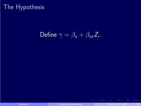
The Hypothesis
Define γ = βx + βxzZi .
Boehmke Interactions Workshop February 29, 2008 4 / 40
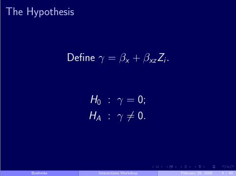
The Hypothesis
Define γ = βx + βxzZi .
H0 : γ = 0;
HA : γ 6= 0.
Boehmke Interactions Workshop February 29, 2008 4 / 40
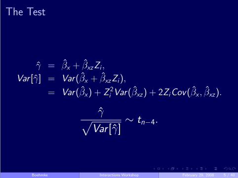
The Test
γ̂ = β̂x + β̂xzZi ,
Var [γ̂] = Var(β̂x + β̂xzZi),
= Var(β̂x) + Z 2
i Var(β̂xz) + 2ZiCov(β̂x , β̂xz).
γ̂√
Var [γ̂]∼ tn−4.
Boehmke Interactions Workshop February 29, 2008 5 / 40

Frequently Overhead
1 I don’t need to include Xi .
Boehmke Interactions Workshop February 29, 2008 6 / 40

Frequently Overhead
1 I don’t need to include Xi .2 I can interpret β̂x directly.
Boehmke Interactions Workshop February 29, 2008 6 / 40

Frequently Overhead
1 I don’t need to include Xi .2 I can interpret β̂x directly.3 The coefficients are not significant.
Boehmke Interactions Workshop February 29, 2008 6 / 40
I Don’t Need to Include X
1 Maybe you have no prediction about its direct effect.
Boehmke Interactions Workshop February 29, 2008 7 / 40
I Don’t Need to Include X
1 Maybe you have no prediction about its direct effect.2 Maybe you have a theory that says its direct effect
is zero.
Boehmke Interactions Workshop February 29, 2008 7 / 40
I Don’t Need to Include X
1 Maybe you have no prediction about its direct effect.2 Maybe you have a theory that says its direct effect
is zero.3 Maybe you have a lot of correlation between X and
X × Z .
Boehmke Interactions Workshop February 29, 2008 7 / 40
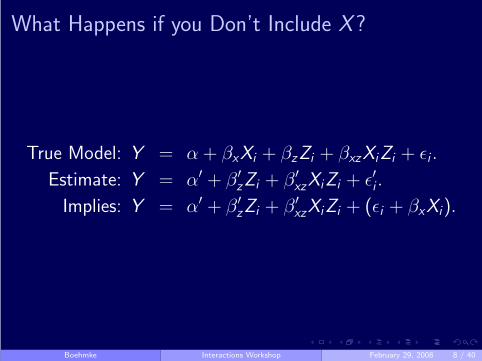
What Happens if you Don’t Include X ?
True Model: Y = α + βxXi + βzZi + βxzXiZi + εi .
Estimate: Y = α′ + β′zZi + β′
xzXiZi + ε′i .
Implies: Y = α′ + β′zZi + β′
xzXiZi + (εi + βxXi).
Boehmke Interactions Workshop February 29, 2008 8 / 40
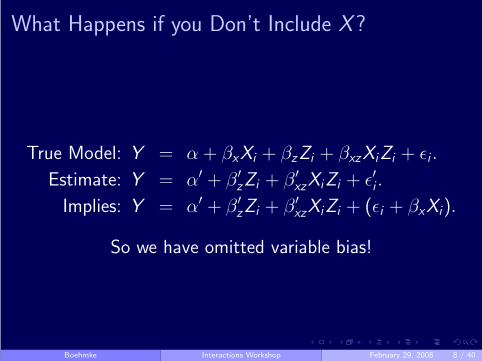
What Happens if you Don’t Include X ?
True Model: Y = α + βxXi + βzZi + βxzXiZi + εi .
Estimate: Y = α′ + β′zZi + β′
xzXiZi + ε′i .
Implies: Y = α′ + β′zZi + β′
xzXiZi + (εi + βxXi).
So we have omitted variable bias!
Boehmke Interactions Workshop February 29, 2008 8 / 40
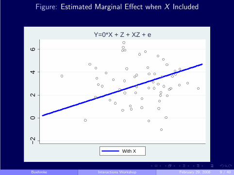
Figure: Estimated Marginal Effect when X Included
−2
02
46
With X
Y=0*X + Z + XZ + e
Boehmke Interactions Workshop February 29, 2008 9 / 40
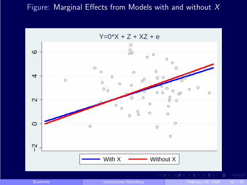
Figure: Marginal Effects from Models with and without X
−2
02
46
With X Without X
Y=0*X + Z + XZ + e
Boehmke Interactions Workshop February 29, 2008 10 / 40
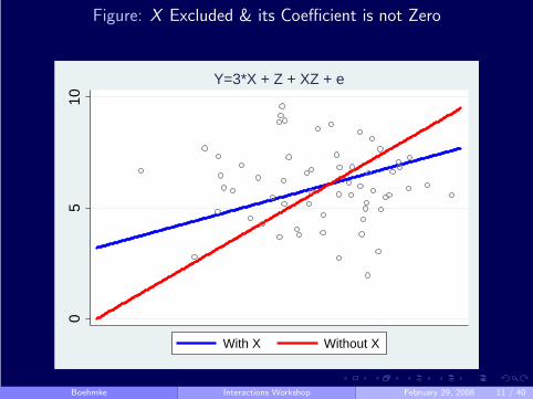
Figure: X Excluded & its Coefficient is not Zero
05
10
With X Without X
Y=3*X + Z + XZ + e
Boehmke Interactions Workshop February 29, 2008 11 / 40
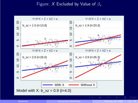
Figure: X Excluded by Value of βx
b_xz = 1.0 (t=13.8)
05
1015
20Y=0*X + Z + XZ + e
b_xz = 1.9 (t=23.3)
05
1015
20
Y=3*X + Z + XZ + e
b_xz = 2.9 (t=26.0)
05
1015
20
Y=6*X + Z + XZ + e
b_xz = 3.9 (t=26.3)
05
1015
20
Y=9*X + Z + XZ + e
Model with X: b_xz = 0.9 (t=4.0)
With X Without X
Boehmke Interactions Workshop February 29, 2008 12 / 40
Figure: It Gets Worse!
Boehmke Interactions Workshop February 29, 2008 13 / 40
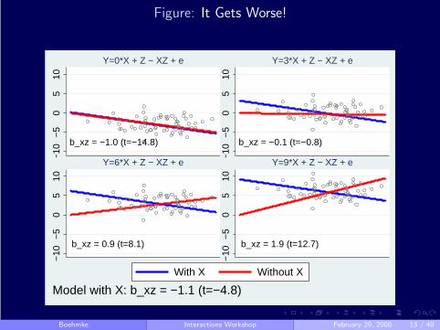
Figure: It Gets Worse!
b_xz = −1.0 (t=−14.8)
−10
−5
05
10Y=0*X + Z − XZ + e
b_xz = −0.1 (t=−0.8)
−10
−5
05
10
Y=3*X + Z − XZ + e
b_xz = 0.9 (t=8.1)
−10
−5
05
10
Y=6*X + Z − XZ + e
b_xz = 1.9 (t=12.7)
−10
−5
05
10
Y=9*X + Z − XZ + e
Model with X: b_xz = −1.1 (t=−4.8)
With X Without X
Boehmke Interactions Workshop February 29, 2008 13 / 40
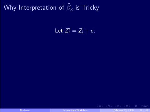
Why Interpretation of β̂x is Tricky
Let Z ′i = Zi + c .
Boehmke Interactions Workshop February 29, 2008 14 / 40
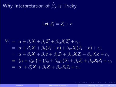
Why Interpretation of β̂x is Tricky
Let Z ′i = Zi + c .
Yi = α + βxXi + βzZ′i + βxzXiZ
′i + εi ,
= α + βxXi + βz(Zi + c) + βxzXi(Zi + c) + εi ,
= α + βxXi + βzc + βzZi + βxzXiZi + βxzXic + εi ,
= (α + βzc) + (βx + βxzc)Xi + βzZi + βxzXiZi + εi ,
= α′ + β′xXi + βzZi + βxzXiZi + εi .
Boehmke Interactions Workshop February 29, 2008 14 / 40
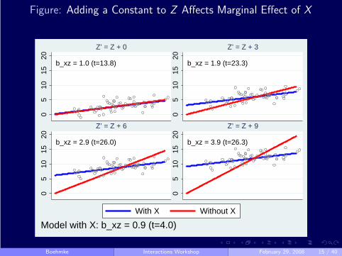
Figure: Adding a Constant to Z Affects Marginal Effect of X
b_xz = 1.0 (t=13.8)
05
1015
20Z’ = Z + 0
b_xz = 1.9 (t=23.3)
05
1015
20
Z’ = Z + 3
b_xz = 2.9 (t=26.0)
05
1015
20
Z’ = Z + 6
b_xz = 3.9 (t=26.3)
05
1015
20
Z’ = Z + 9
Model with X: b_xz = 0.9 (t=4.0)
With X Without X
Boehmke Interactions Workshop February 29, 2008 15 / 40

Just Look at the Significance of the Coefficients
Coefficients possess only limited information.
Boehmke Interactions Workshop February 29, 2008 16 / 40

Just Look at the Significance of the Coefficients
Coefficients possess only limited information.
As we’ve seen, coefficients on constitutive terms aremeaningless.
Boehmke Interactions Workshop February 29, 2008 16 / 40

Just Look at the Significance of the Coefficients
Coefficients possess only limited information.
As we’ve seen, coefficients on constitutive terms aremeaningless.
Need to test whether marginal effect is significant atdifferent values of Z .
Boehmke Interactions Workshop February 29, 2008 16 / 40

Table: Number of Citizen Interest Groups per State, 1990
Initiative State 88.50 ∗ ∗ 85.24(41.72) (93.45)
Total Population 17.53 ∗ ∗ 17.56 ∗ ∗(3.92) (4.04)
Citizen Ideology 1.89 2.02(2.88) (4.34)
Initiative × Ideology −0.23(5.83)
Constant 80.54 82.15(56.38) (70.23)
Boehmke Interactions Workshop February 29, 2008 17 / 40
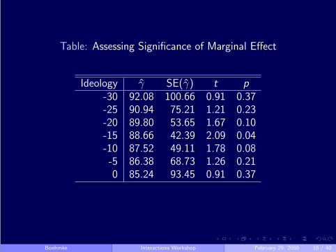
Table: Assessing Significance of Marginal Effect
Ideology γ̂ SE(γ̂) t p
-30 92.08 100.66 0.91 0.37-25 90.94 75.21 1.21 0.23-20 89.80 53.65 1.67 0.10-15 88.66 42.39 2.09 0.04-10 87.52 49.11 1.78 0.08-5 86.38 68.73 1.26 0.210 85.24 93.45 0.91 0.37
Boehmke Interactions Workshop February 29, 2008 18 / 40
Implementing Interaction Tests in Stata
1 Using Stata’s test command.
Boehmke Interactions Workshop February 29, 2008 19 / 40
Implementing Interaction Tests in Stata
1 Using Stata’s test command.
2 Using Clarify suite.
Boehmke Interactions Workshop February 29, 2008 19 / 40
Implementing Interaction Tests in Stata
1 Using Stata’s test command.
2 Using Clarify suite.
3 Using grinter.
Boehmke Interactions Workshop February 29, 2008 19 / 40
Implementing Interaction Tests in Stata
1 Using Stata’s test command.
2 Using Clarify suite.
3 Using grinter.
4 Using formulas.
Boehmke Interactions Workshop February 29, 2008 19 / 40
Implementing Interaction Tests in Stata
1 Using Stata’s test command.
2 Using Clarify suite.
3 Using grinter.
4 Using formulas.
5 Using simulations.
Boehmke Interactions Workshop February 29, 2008 19 / 40
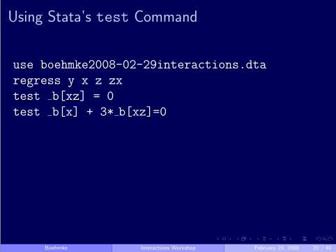
Using Stata’s test Command
use boehmke2008-02-29interactions.dta
regress y x z zx
test b[xz] = 0
test b[x] + 3* b[xz]=0
Boehmke Interactions Workshop February 29, 2008 20 / 40
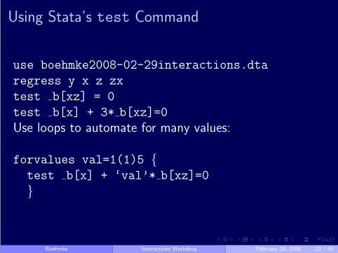
Using Stata’s test Command
use boehmke2008-02-29interactions.dta
regress y x z zx
test b[xz] = 0
test b[x] + 3* b[xz]=0
Use loops to automate for many values:
forvalues val=1(1)5 {test b[x] + ‘val’* b[xz]=0
}
Boehmke Interactions Workshop February 29, 2008 20 / 40
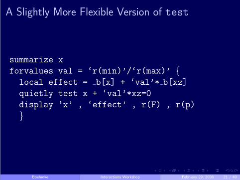
A Slightly More Flexible Version of test
summarize x
forvalues val = ‘r(min)’/‘r(max)’ {local effect = b[x] + ‘val’* b[xz]
quietly test x + ‘val’*xz=0
display ‘x’ , ‘effect’ , r(F) , r(p)
}
Boehmke Interactions Workshop February 29, 2008 21 / 40
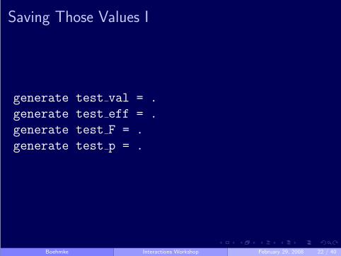
Saving Those Values I
generate test val = .
generate test eff = .
generate test F = .
generate test p = .
Boehmke Interactions Workshop February 29, 2008 22 / 40
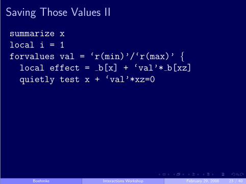
Saving Those Values II
summarize x
local i = 1
forvalues val = ‘r(min)’/‘r(max)’ {local effect = b[x] + ‘val’* b[xz]
quietly test x + ‘val’*xz=0
Boehmke Interactions Workshop February 29, 2008 23 / 40
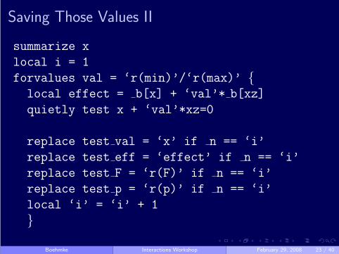
Saving Those Values II
summarize x
local i = 1
forvalues val = ‘r(min)’/‘r(max)’ {local effect = b[x] + ‘val’* b[xz]
quietly test x + ‘val’*xz=0
replace test val = ‘x’ if n == ‘i’
replace test eff = ‘effect’ if n == ‘i’
replace test F = ‘r(F)’ if n == ‘i’
replace test p = ‘r(p)’ if n == ‘i’
local ‘i’ = ‘i’ + 1
}
Boehmke Interactions Workshop February 29, 2008 23 / 40
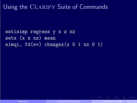
Using the Clarify Suite of Commands
estisimp regress y x z xz
setx (x z xz) mean
simqi, fd(ev) changex(x 0 1 xz 0 1)
Boehmke Interactions Workshop February 29, 2008 24 / 40
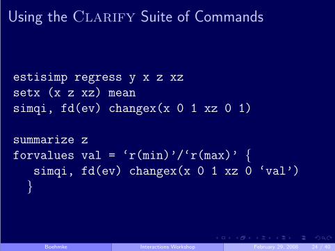
Using the Clarify Suite of Commands
estisimp regress y x z xz
setx (x z xz) mean
simqi, fd(ev) changex(x 0 1 xz 0 1)
summarize z
forvalues val = ‘r(min)’/‘r(max)’ {simqi, fd(ev) changex(x 0 1 xz 0 ‘val’)
}
Boehmke Interactions Workshop February 29, 2008 24 / 40

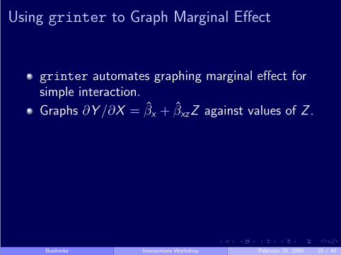
Using grinter to Graph Marginal Effect
grinter automates graphing marginal effect forsimple interaction.
Boehmke Interactions Workshop February 29, 2008 25 / 40
Using grinter to Graph Marginal Effect
grinter automates graphing marginal effect forsimple interaction.
Graphs ∂Y /∂X = β̂x + β̂xzZ against values of Z .
Boehmke Interactions Workshop February 29, 2008 25 / 40
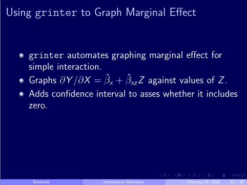
Using grinter to Graph Marginal Effect
grinter automates graphing marginal effect forsimple interaction.
Graphs ∂Y /∂X = β̂x + β̂xzZ against values of Z .
Adds confidence interval to asses whether it includeszero.
Boehmke Interactions Workshop February 29, 2008 25 / 40
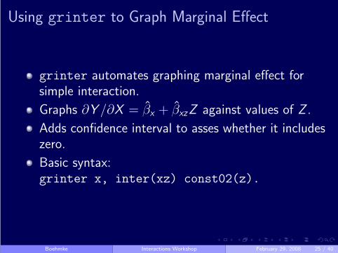
Using grinter to Graph Marginal Effect
grinter automates graphing marginal effect forsimple interaction.
Graphs ∂Y /∂X = β̂x + β̂xzZ against values of Z .
Adds confidence interval to asses whether it includeszero.
Basic syntax:grinter x, inter(xz) const02(z).
Boehmke Interactions Workshop February 29, 2008 25 / 40
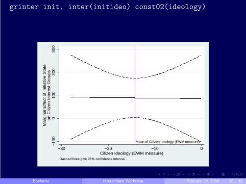
grinter init, inter(initideo) const02(ideology)
Mean of Citizen Ideology (EWM measure)
−10
00
100
200
300
Mar
gina
l Effe
ct o
f Ini
tiativ
e S
tate
on C
itize
n In
tere
st G
roup
s
−30 −20 −10 0Citizen Ideology (EWM measure)
Dashed lines give 95% confidence interval.
Boehmke Interactions Workshop February 29, 2008 26 / 40
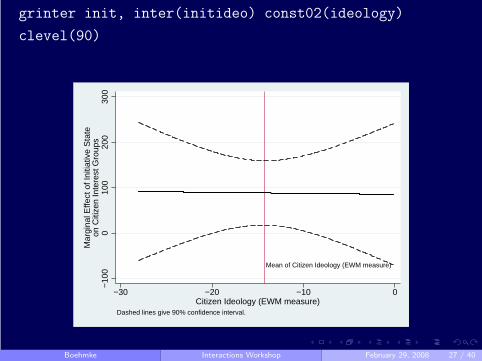
grinter init, inter(initideo) const02(ideology)
clevel(90)
Mean of Citizen Ideology (EWM measure)
−10
00
100
200
300
Mar
gina
l Effe
ct o
f Ini
tiativ
e S
tate
on C
itize
n In
tere
st G
roup
s
−30 −20 −10 0Citizen Ideology (EWM measure)
Dashed lines give 90% confidence interval.
Boehmke Interactions Workshop February 29, 2008 27 / 40
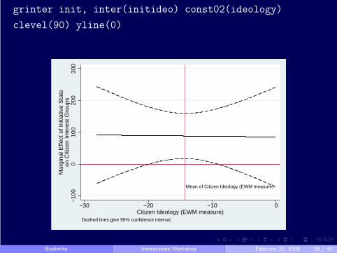
grinter init, inter(initideo) const02(ideology)
clevel(90) yline(0)
Mean of Citizen Ideology (EWM measure)
−10
00
100
200
300
Mar
gina
l Effe
ct o
f Ini
tiativ
e S
tate
on C
itize
n In
tere
st G
roup
s
−30 −20 −10 0Citizen Ideology (EWM measure)
Dashed lines give 90% confidence interval.
Boehmke Interactions Workshop February 29, 2008 28 / 40
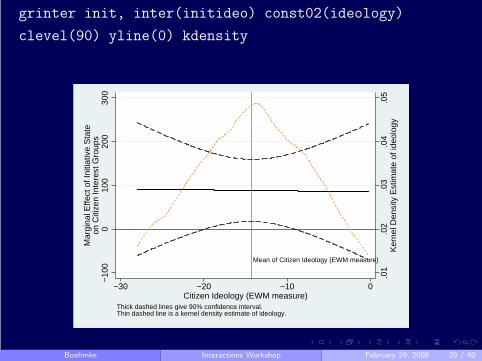
grinter init, inter(initideo) const02(ideology)
clevel(90) yline(0) kdensity
Mean of Citizen Ideology (EWM measure)
.01
.02
.03
.04
.05
Ker
nel D
ensi
ty E
stim
ate
of id
eolo
gy
−10
00
100
200
300
Mar
gina
l Effe
ct o
f Ini
tiativ
e S
tate
on C
itize
n In
tere
st G
roup
s
−30 −20 −10 0Citizen Ideology (EWM measure)
Thick dashed lines give 90% confidence interval.Thin dashed line is a kernel density estimate of ideology.
Boehmke Interactions Workshop February 29, 2008 29 / 40

Figure: A More Complicated Example
−15
−10
−5
05
Mar
gina
l Effe
ct
0 .1 .2 .3 .4 .5Legislative Professionalism
Severe Deficiencies
Boehmke Interactions Workshop February 29, 2008 30 / 40
Marginal Effects in Non-Linear Models
More difficult than in OLS since marginal effectdepends on all covariates.
Boehmke Interactions Workshop February 29, 2008 31 / 40

Marginal Effects in Non-Linear Models
More difficult than in OLS since marginal effectdepends on all covariates.
But the basic principle remains the same: determine
∂Y /∂X .
Boehmke Interactions Workshop February 29, 2008 31 / 40
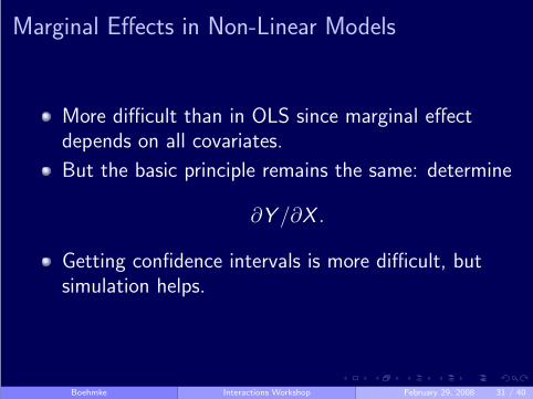
Marginal Effects in Non-Linear Models
More difficult than in OLS since marginal effectdepends on all covariates.
But the basic principle remains the same: determine
∂Y /∂X .
Getting confidence intervals is more difficult, butsimulation helps.
Boehmke Interactions Workshop February 29, 2008 31 / 40
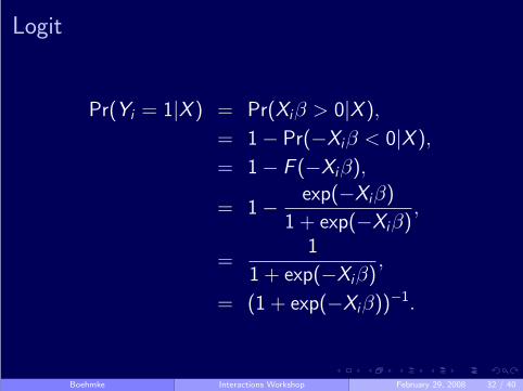
Logit
Pr(Yi = 1|X ) = Pr(Xiβ > 0|X ),
= 1 − Pr(−Xiβ < 0|X ),
= 1 − F (−Xiβ),
= 1 −exp(−Xiβ)
1 + exp(−Xiβ),
=1
1 + exp(−Xiβ),
= (1 + exp(−Xiβ))−1.
Boehmke Interactions Workshop February 29, 2008 32 / 40
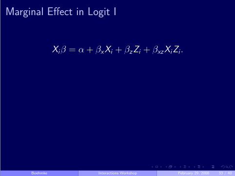
Marginal Effect in Logit I
Xiβ = α + βxXi + βzZi + βxzXiZi .
Boehmke Interactions Workshop February 29, 2008 33 / 40
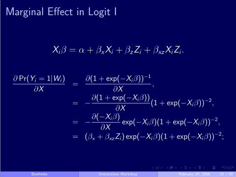
Marginal Effect in Logit I
Xiβ = α + βxXi + βzZi + βxzXiZi .
∂ Pr(Yi = 1|Wi)
∂X=
∂(1 + exp(−Xiβ))−1
∂X,
= −∂(1 + exp(−Xiβ))
∂X(1 + exp(−Xiβ))−2,
= −∂(−Xiβ)
∂Xexp(−Xiβ)(1 + exp(−Xiβ))−2,
= (βx + βxzZi) exp(−Xiβ)(1 + exp(−Xiβ))−2;
Boehmke Interactions Workshop February 29, 2008 33 / 40
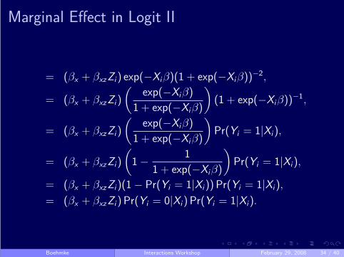
Marginal Effect in Logit II
= (βx + βxzZi) exp(−Xiβ)(1 + exp(−Xiβ))−2,
= (βx + βxzZi)
(
exp(−Xiβ)
1 + exp(−Xiβ)
)
(1 + exp(−Xiβ))−1,
= (βx + βxzZi)
(
exp(−Xiβ)
1 + exp(−Xiβ)
)
Pr(Yi = 1|Xi),
= (βx + βxzZi)
(
1 −1
1 + exp(−Xiβ)
)
Pr(Yi = 1|Xi),
= (βx + βxzZi)(1 − Pr(Yi = 1|Xi)) Pr(Yi = 1|Xi),
= (βx + βxzZi) Pr(Yi = 0|Xi) Pr(Yi = 1|Xi).
Boehmke Interactions Workshop February 29, 2008 34 / 40
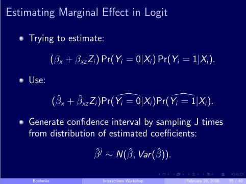
Estimating Marginal Effect in Logit
Trying to estimate:
(βx + βxzZi) Pr(Yi = 0|Xi) Pr(Yi = 1|Xi).
Use:
(β̂x + β̂xzZi) ̂Pr(Yi = 0|Xi) ̂Pr(Yi = 1|Xi).
Generate confidence interval by sampling J timesfrom distribution of estimated coefficients:
β̂j ∼ N(β̂, Var(β̂)).
Boehmke Interactions Workshop February 29, 2008 35 / 40
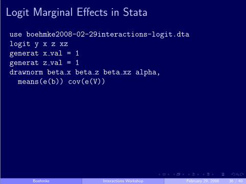
Logit Marginal Effects in Stata
use boehmke2008-02-29interactions-logit.dta
logit y x z xz
generat x val = 1
generat z val = 1
drawnorm beta x beta z beta xz alpha,
means(e(b)) cov(e(V))
Boehmke Interactions Workshop February 29, 2008 36 / 40
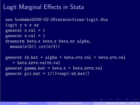
Logit Marginal Effects in Stata
use boehmke2008-02-29interactions-logit.dta
logit y x z xz
generat x val = 1
generat z val = 1
drawnorm beta x beta z beta xz alpha,
means(e(b)) cov(e(V))
generat xb hat = alpha + beta x*x val + beta z*z val
+ beta xz*x val*z val
generat gamma hat = beta x + beta xz*z val
generat pi1 hat = 1/(1+exp(-xb hat))
Boehmke Interactions Workshop February 29, 2008 36 / 40
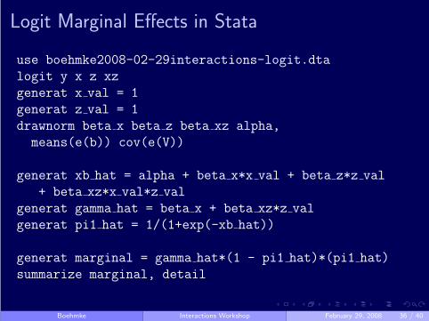
Logit Marginal Effects in Stata
use boehmke2008-02-29interactions-logit.dta
logit y x z xz
generat x val = 1
generat z val = 1
drawnorm beta x beta z beta xz alpha,
means(e(b)) cov(e(V))
generat xb hat = alpha + beta x*x val + beta z*z val
+ beta xz*x val*z val
generat gamma hat = beta x + beta xz*z val
generat pi1 hat = 1/(1+exp(-xb hat))
generat marginal = gamma hat*(1 - pi1 hat)*(pi1 hat)
summarize marginal, detail
Boehmke Interactions Workshop February 29, 2008 36 / 40
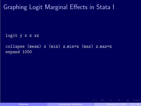
Graphing Logit Marginal Effects in Stata I
logit y x z xz
collapse (mean) x (min) z min=z (max) z max=z
expand 1000
Boehmke Interactions Workshop February 29, 2008 37 / 40
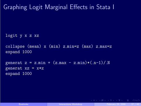
Graphing Logit Marginal Effects in Stata I
logit y x z xz
collapse (mean) x (min) z min=z (max) z max=z
expand 1000
generat z = z min + (z max - z min)*( n-1)/ N
generat xz = x*z
expand 1000
Boehmke Interactions Workshop February 29, 2008 37 / 40
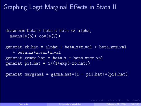
Graphing Logit Marginal Effects in Stata II
drawnorm beta x beta z beta xz alpha,
means(e(b)) cov(e(V))
generat xb hat = alpha + beta x*x val + beta z*z val
+ beta xz*x val*z val
generat gamma hat = beta x + beta xz*z val
generat pi1 hat = 1/(1+exp(-xb hat))
generat marginal = gamma hat*(1 - pi1 hat)*(pi1 hat)
Boehmke Interactions Workshop February 29, 2008 38 / 40

Graphing Logit Marginal Effects in Stata III
collapse (mean) marginal (p5) marg lb=marginal (p95)
marg ub=marginal, by(z)
Boehmke Interactions Workshop February 29, 2008 39 / 40
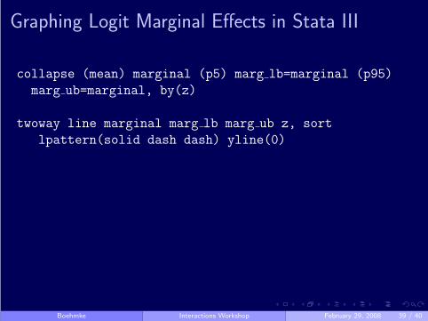
Graphing Logit Marginal Effects in Stata III
collapse (mean) marginal (p5) marg lb=marginal (p95)
marg ub=marginal, by(z)
twoway line marginal marg lb marg ub z, sort
lpattern(solid dash dash) yline(0)
Boehmke Interactions Workshop February 29, 2008 39 / 40
Graphing Logit Marginal Effects in Stata III
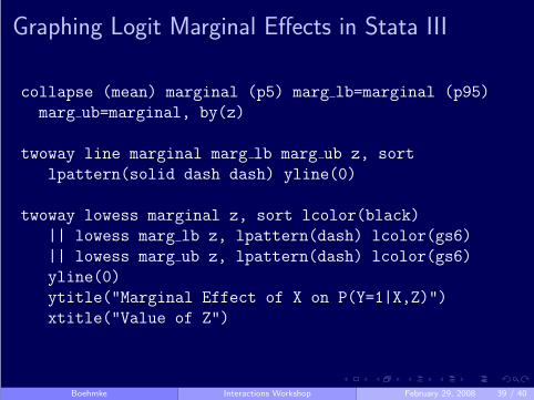
collapse (mean) marginal (p5) marg lb=marginal (p95)
marg ub=marginal, by(z)
twoway line marginal marg lb marg ub z, sort
lpattern(solid dash dash) yline(0)
twoway lowess marginal z, sort lcolor(black)
|| lowess marg lb z, lpattern(dash) lcolor(gs6)
|| lowess marg ub z, lpattern(dash) lcolor(gs6)
yline(0)
ytitle("Marginal Effect of X on P(Y=1|X,Z)")
xtitle("Value of Z")
Boehmke Interactions Workshop February 29, 2008 39 / 40
Conclusion
Lots of bias can emerge if constitutive terms notincluded.
Boehmke Interactions Workshop February 29, 2008 40 / 40
Conclusion
Lots of bias can emerge if constitutive terms notincluded.
Even if you have a theory, probably best to includethem.
Boehmke Interactions Workshop February 29, 2008 40 / 40
Conclusion
Lots of bias can emerge if constitutive terms notincluded.
Even if you have a theory, probably best to includethem.
Many ways to assess significance.
Boehmke Interactions Workshop February 29, 2008 40 / 40
Conclusion
Lots of bias can emerge if constitutive terms notincluded.
Even if you have a theory, probably best to includethem.
Many ways to assess significance.
Same principle allows calculation for any estimatoror form of interactions.
Boehmke Interactions Workshop February 29, 2008 40 / 40