interpreting regression models · web viewdraft: long-statacorp-2013-08-07.docx interpreting...

Indiana University

Interpreting regression models using Stata Scott Long August 13, 2013 Draft: document.docx.docx

Interpreting regression models

1980s Interpreting log-linear and multinomial

models to support substantive research

1991 Markov: A Statistical Environment for GAUSS

1996 change.ado and genpred.ado in Stata 4

1997 Regression Models for Categorical and Limited

Dependent Variables

1997 Markov 2.5

Page 1

Working with StataCorp

1998 Bill Sribney on post-estimationBill Gould on returns

1999 SPost with Jeremy Freese

2000 David Drukker and StataPress

2001 Regression Models for Categorical Dependent Variables with Statawith Jeremy Freese.

Page 2

Continuing work...2005 Regression Models with Stata, 2nd

2005 SPost9 20,000 downloads.

2008 The Workflow of Data Analysis using Stata

2009 Stata 11 and margins and factor variables.

2011 Stata 12 with marginsplot2012 SPost13 for 3rd edition

2013 Stata 13

Page 3

Stata at IndianaMy students appeared in class wearing...

Page 4

Goals for visiting StataCorpDemo SPost13 wrappers for marginso Did we miss something? Are there better ways to do things?

o Do our new methods of interpretation make sense?

Other SPost13 commandso Why we wrote themo Why StataCorp might want to improve them

Things we'd like to see in Stata

Page 5

Interpretation using predictions

With multiple outcomes and K predictors...

Page 6

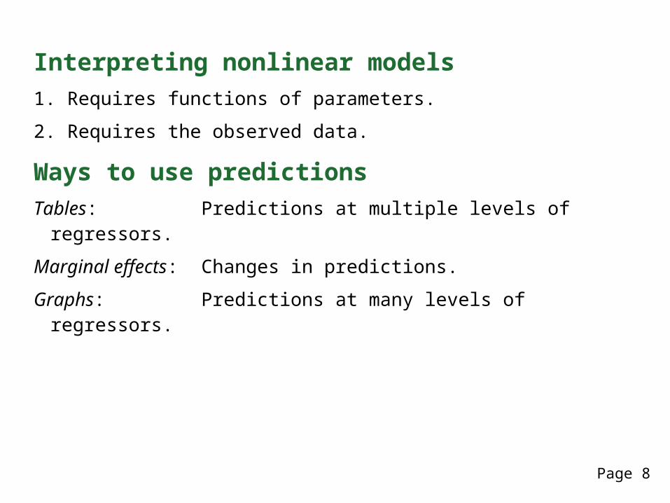
Interpreting nonlinear models1. Requires functions of parameters.

2. Requires the observed data.

Ways to use predictionsTables: Predictions at multiple levels of regressors.

Marginal effects: Changes in predictions.

Graphs: Predictions at many levels of regressors.

Page 7

The toolsOfficial Statamarginsmarginsplot

SPost13 wrappers for margins and lincommtable: tables of predictions

mchange: marginal effects

mgen: predictions to plot

mlistat: compact at() matrix listing

mlincom: tables of linear combinations (wrapper for lincom)

Why not simply use margins and marginsplot?

Page 8

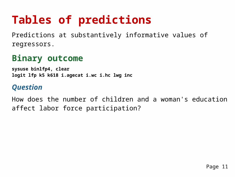
Tables of predictionsPredictions at substantively informative values of regressors.

Binary outcomesysuse binlfp4, clearlogit lfp k5 k618 i.agecat i.wc i.hc lwg inc

Question

How does the number of children and a woman's education affect labor force participation?

Page 9

margins. margins, atmeans at(wc=(0 1) k5=(0 1 2 3))

Adjusted predictions Number of obs = 753Model VCE : OIM

Expression : Pr(lfp), predict()

1._at : wc = 0 k5 = 0 k618 = 1.353254 (mean) 1.agecat = .3957503 (mean) 2.agecat = .3851262 (mean) 3.agecat = .2191235 (mean) 0.hc = .6082337 (mean) 1.hc = .3917663 (mean) lwg = 1.097115 (mean) inc = 20.12897 (mean)

2._at : wc = 0:::snip:::3._at : wc = 0:::snip:::4._at : wc = 0:::snip:::5._at : wc = 1:::snip:::

Page 10

6._at : wc = 1:::snip:::7._at : wc = 1:::snip:::8._at : wc = 1:::snip:::

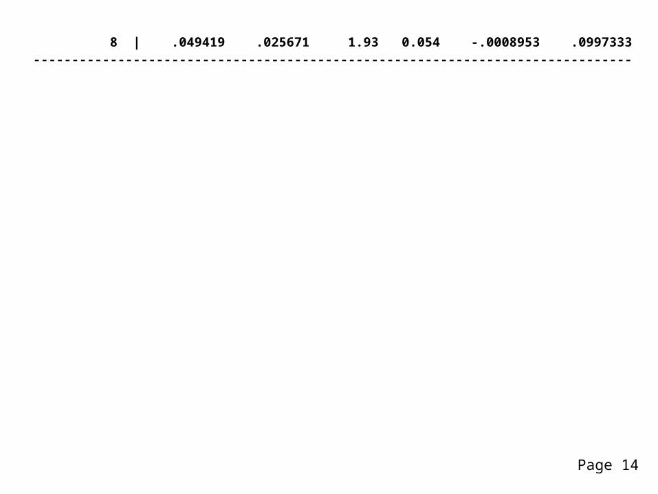
------------------------------------------------------------------------------ | Delta-method | Margin Std. Err. z P>|z| [95% Conf. Interval]-------------+---------------------------------------------------------------- _at | 1 | .6035431 .0256741 23.51 0.000 .5532229 .6538633 2 | .2746181 .0359919 7.63 0.000 .2040752 .3451609 3 | .0860471 .0280757 3.06 0.002 .0310198 .1410744 4 | .0228776 .0121605 1.88 0.060 -.0009566 .0467119 5 | .771705 .0349691 22.07 0.000 .7031668 .8402432 6 | .4567078 .0566536 8.06 0.000 .3456687 .5677469 7 | .1729059 .0532296 3.25 0.001 .0685779 .277234 8 | .049419 .025671 1.93 0.054 -.0008953 .0997333------------------------------------------------------------------------------

Page 11

mtable: simple. mtable, atmeans at(wc=(0 1) k5=(0 1 2 3)) <= pass through to margins

Expression: Pr(lfp)

| 1. | wc k5 pr ----------+----------------------------- 1 | 0 0 0.604 2 | 0 1 0.275 3 | 0 2 0.086 4 | 0 3 0.023 5 | 1 0 0.772 6 | 1 1 0.457 7 | 1 2 0.173 8 | 1 3 0.049

Constant values of at() variables

2. 3. 1. k618 agecat agecat hc lwg inc ----------------------------------------------------------------- 1.353 0.385 0.219 0.392 1.097 20.129

Page 12

mtable: building a table. qui mtable, atmeans at(wc=0 k5=(0 1 2 3)) estname(NoCol)

. qui mtable, atmeans at(wc=1 k5=(0 1 2 3)) estname(College) ///> atvars(_none) right

. mtable, atmeans dydx(wc) at(k5=(0 1 2 3)) estname(Diff) stats(est p) ///> atvars(_none) names(columns) right

k5 NoCol College Diff p------------------------------------------------ 0 0.604 0.772 0.168 0.000 1 0.275 0.457 0.182 0.001 2 0.086 0.173 0.087 0.013 3 0.023 0.049 0.027 0.085

Page 13

margins. foreach iout in 1 2 3 4 { 2. margins, at(yr89=(0 1) male=(0 1)) atmeans predict(outcome(`iout')) 3. }


Expression : Pr(warm==1), predict(outcome(1))

1._at : yr89 = 0:::snip:::------------------------------------------------------------------------------ | Delta-method | Margin Std. Err. z P>|z| [95% Conf. Interval]-------------+---------------------------------------------------------------- _at | 1 | .0981207 .0074061 13.25 0.000 .083605 .1126365 2 | .1868221 .0117184 15.94 0.000 .1638545 .2097897 3 | .0604381 .0053787 11.24 0.000 .049896 .0709802 4 | .1195914 .0095217 12.56 0.000 .1009293 .1382536------------------------------------------------------------------------------

Page 15


Expression : Pr(warm==2), predict(outcome(2)):::snip:::

------------------------------------------------------------------------------ | Delta-method | Margin Std. Err. z P>|z| [95% Conf. Interval]-------------+---------------------------------------------------------------- _at | 1 | .3069102 .0125571 24.44 0.000 .2822987 .3315216 2 | .4029306 .0127015 31.72 0.000 .378036 .4278251 3 | .2265499 .0119914 18.89 0.000 .2030473 .2500525 4 | .3398556 .0137531 24.71 0.000 .3129002 .3668111------------------------------------------------------------------------------

:::snip:::

:::snip:::

Page 16

mtable: quick. mtable, at(yr89=(0 1) male=(0 1)) atmeans

Expression: Pr(warm)

| 1. 1. | yr89 male 1 SD 2 D 3 A 4 SA ----------+----------------------------------------------------------- 1 | 0 0 0.098 0.307 0.415 0.180 2 | 0 1 0.187 0.403 0.316 0.094 3 | 1 0 0.060 0.227 0.442 0.271 4 | 1 1 0.120 0.340 0.391 0.150

Constant values of at() variables

1. 2. 3. 4. white age edcat edcat edcat prst----------------------------------------------------------------- 0.877 44.935 0.341 0.196 0.171 39.585

Page 17

mtable: building. qui mtable, at(yr89=0 male=1) atmeans rowname(Men) clear roweq(1977). qui mtable, at(yr89=0 male=0) atmeans rowname(Women) below roweq(1977). qui mtable, dydx(male) at(yr89=0) atmeans rowname(M-W) below roweq(1977)

. qui mtable, at(yr89=1 male=1) atmeans rowname(Men) below roweq(1989)

. qui mtable, at(yr89=1 male=0) atmeans rowname(Women) below roweq(1989)

. qui mtable, dydx(male) at(yr89=1) atmeans rowname(M-W) below roweq(1989)

. qui mtable, dydx(yr89) at(male=1) atmeans rowname(77to89) below roweq(Men)

. mtable, dydx(yr89) at(male=0) atmeans rowname(77to89) below roweq(Women)

| 1 SD 2 D 3 A 4 SA ----------+--------------------------------------- 1977 | Men | 0.187 0.403 0.316 0.094 Women | 0.098 0.307 0.415 0.180 M-W | 0.089 0.096 -0.099 -0.086 1989 | Men | 0.120 0.340 0.391 0.150 Women | 0.060 0.227 0.442 0.271 M-W | 0.059 0.113 -0.051 -0.121 Men | 77to89 | -0.067 -0.063 0.075 0.055 Women | 77to89 | -0.038 -0.080 0.027 0.091

Page 18

SUGGESTION 1.margins for multiple outcomes

o Joint estimation, not simply accumulation over outcomes

2. Compact summary of at() values.

Page 19

Marginal effects

Pr(y=1|x)x Pr(y=1|x)

x

Pr(

y=1|

x)

x x+1brm_dc_partial.do jsl 2013-04-12

Mathematically, ...

Page 20

Marginal change

Discrete change

Page 21

Binary outcomesysuse binlfp4, clearlogit lfp k5 k618 i.agecat i.wc i.hc lwg inc

Question

How to assess the magnitudes of the effects?

mchange. mchange

logit: Changes in Pr(lfp) | N = 753

| Change P>|z|----------------+----------------------1.wc | 0 to 1 | 0.1624 0.0002 k5 | +1 cntr | -0.2818 0.0000 +SD cntr | -0.1503 0.0000 Marginal | -0.2888 0.0000 k618 | +1 cntr | -0.0136 0.3354 +SD cntr | -0.0180 0.3353

Page 22

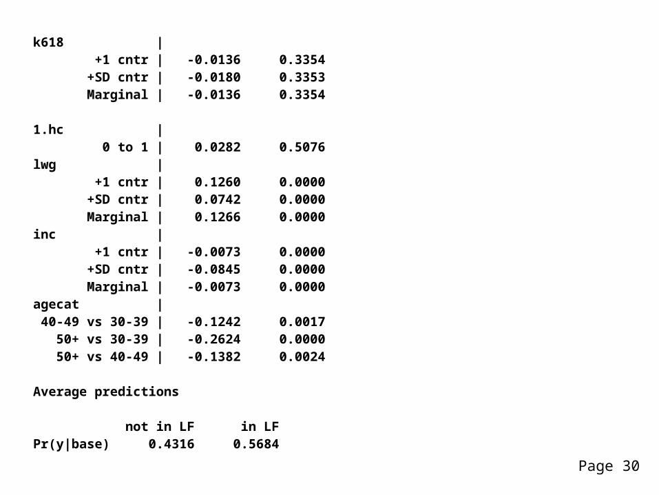
Marginal | -0.0136 0.3354

1.hc | 0 to 1 | 0.0282 0.5076 lwg | +1 cntr | 0.1260 0.0000 +SD cntr | 0.0742 0.0000 Marginal | 0.1266 0.0000 inc | +1 cntr | -0.0073 0.0000 +SD cntr | -0.0845 0.0000 Marginal | -0.0073 0.0000 agecat | 40-49 vs 30-39 | -0.1242 0.0017 50+ vs 30-39 | -0.2624 0.0000 50+ vs 40-49 | -0.1382 0.0024

Average predictions

not in LF in LFPr(y|base) 0.4316 0.5684

1: Predictions averaged over the sample.

Page 23

mchange with options (edited). mchange, stats(from to change pvalue)

logit: Changes in Pr(lfp) | N = 753

| From To Change P>|z|----------------+--------------------------------------------1.wc | 0 to 1 | 0.5251 0.6875 0.1624 0.0002 k5 | +1 cntr | 0.7040 0.4222 -0.2818 0.0000 +SD cntr | 0.6420 0.4917 -0.1503 0.0000 Marginal | . . -0.2888 0.0000 inc | +1 cntr | 0.5720 0.5648 -0.0073 0.0000 +SD cntr | 0.6101 0.5257 -0.0845 0.0000 Marginal | . . -0.0073 0.0000 agecat | 40-49 vs 30-39 | 0.5521 0.6764 -0.1242 0.0017 50+ vs 30-39 | 0.4139 0.6764 -0.2624 0.0000 50+ vs 40-49 | 0.4139 0.5521 -0.1382 0.0024

Average predictions

not in LF in LFPr(y|base) 0.4316 0.5684

Page 24


Page 25

marginsmargins, at(k5=gen(k5-.5)) at(k5=gen(k5+.5)) post lincom _b[2._at]-_b[1._at] est restore blmmargins, at(k5=gen(k5-.2619795189419575)) /// at(k5=gen(k5+.2619795189419575)) post lincom _b[2._at]-_b[1._at] est restore blmmargins, dydx(k5)margins, at(k618=gen(k618-.5)) at(k618=gen(k618+.5)) post lincom _b[2._at]-_b[1._at] est restore blmmargins, at(k618=gen(k618-.6599369652141052)) /// at(k618=gen(k618+.6599369652141052)) post lincom _b[2._at]-_b[1._at] est restore blmmargins, dydx(k618)margins, at(wc=(0 1)) post lincom _b[2._at]-_b[1._at] est restore blmmargins, at(hc=(0 1)) post lincom _b[2._at]-_b[1._at] est restore blmmargins, at(lwg=gen(lwg-.5)) at(lwg=gen(lwg+.5)) post lincom _b[2._at]-_b[1._at] est restore blmmargins, at(lwg=gen(lwg-.2937782125573122)) ///

Page 26

at(lwg=gen(lwg+.2937782125573122)) post lincom _b[2._at]-_b[1._at] est restore blmmargins, dydx(lwg)margins, at(inc=gen(inc-.5)) at(inc=gen(inc+.5)) post lincom _b[2._at]-_b[1._at] est restore blmmargins, at(inc=gen(inc-5.817399266696214)) /// at(inc=gen(inc+5.817399266696214)) post lincom _b[2._at]-_b[1._at] est restore blmmargins, dydx(inc)margins agecat, pwcompare

Page 27

dcplot: marginal effect plotter (meplot would be a better name)dcplot, mcolor(rainbow)

12 3 4

1 234

1 234

1234

12 3 4

12 3 4

0 to 1

0 to 1

0 to 1

SD change

SD change

SD change

1.yr89

1.male

1.white

age

ed

prst

-.1 -.05 -.01 .04 .09Discrete Change in Outcome Probability

Page 30

marginsforeach iout in 1 2 3 4 { margins, at(yr89=(0 1) ) post predict(outcome(ìout')) lincom _b[2._at] - _b[1._at] estimate restore olm margins, at(male=(0 1) ) post predict(outcome(ìout')) lincom _b[2._at] - _b[1._at] estimate restore olm margins, at(white=(0 1) ) post predict(outcome(ìout')) lincom _b[2._at] - _b[1._at] estimate restore olm margins, at(age=gen(age - .5) ) at(age=gen(age + .5) ) /// post predict(outcome(ìout')) lincom _b[2._at] - _b[1._at] estimate restore olm margins, at(age=gen(age - 8.389516848965164) ) /// at(age=gen(age + 8.389516848965164) ) post predict(outcome(ìout')) lincom _b[2._at] - _b[1._at] estimate restore olm margins, dydx(age) predict(outcome(ìout')) margins, at(ed=gen(ed - .5) ) at(ed=gen(ed + .5) ) /// post predict(outcome(ìout')) lincom _b[2._at] - _b[1._at] estimate restore olm margins, at(ed=gen(ed - 1.58041337227172) ) /// at(ed=gen(ed + 1.58041337227172) ) post predict(outcome(ìout')) lincom _b[2._at] - _b[1._at]

Page 31

estimate restore olm margins, dydx(ed) predict(outcome(ìout')) margins, at(prst=gen(prst - .5) ) at(prst=gen(prst + .5) ) /// post predict(outcome(ìout')) lincom _b[2._at] - _b[1._at] estimate restore olm margins, at(prst=gen(prst - 7.24612929840372) ) /// at(prst=gen(prst + 7.24612929840372) ) post predict(outcome(ìout')) lincom _b[2._at] - _b[1._at] estimate restore olm margins, dydx(prst) predict(outcome(ìout'))}

Page 32

What logit output might look like | Coef OR P>|z| AME P>|z|-------------+----------------------------------------------lfp | k5 | -1.392 0.249 0.000 -0.150 0.000 k618 | -0.066 0.936 0.336 -0.018 0.335 wc | 0.798 2.220 0.001 0.162 0.000 hc | 0.136 1.146 0.508 0.028 0.508 lwg | 0.610 1.840 0.000 0.074 0.000 inc | -0.035 0.966 0.000 -0.084 0.000 40-49vs30-39 | 1.481 4.396 0.000 -0.124 0.002 50+vs30-39 | 0.854 2.349 0.005 -0.262 0.000 50+vs40-49 | 0.202 1.224 0.500 -0.138 0.002 Constant | 1.014 2.757 0.000

Page 33

AME and MEMA sometimes less than fruitful debate...

MEM

AME

Should you replace one mean with another?o What is the question you are trying to answer?o Maddala's 1980 advice was pretty good.

Page 34

Distribution of ME'sMarginal change for income

AME|

MEM|0

.1.2

.3.4

Frac

tion

-.008 -.006 -.004 -.002 0Marginal change of inc on Pr(LFP)

Page 35

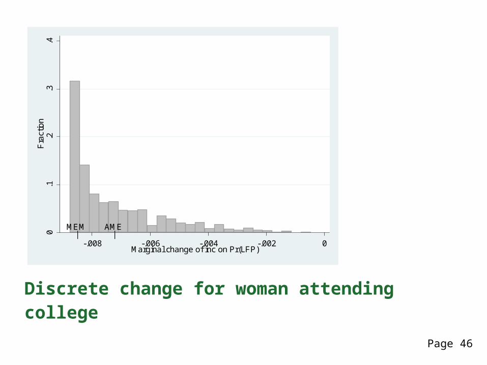
Discrete change for woman attending college

AME|

MEM|0

.1.2

.3Fr

actio

n

0 .05 .1 .15 .2Discrete change of wc on Pr(LFP)

Page 36

Compute marginal effects (not recommended)predict double prhat if e(sample)gen double mcinc = prhat * (1-prhat) * _b[inc]label var mcinc "Marginal change of inc on Pr(LFP)"

Compute effects: with mgen (not recommended)mgen, dydx(wc) over(caseid) stub(wc) noselabel var wcdydx "Discrete change of wc on Pr(LFP)"

Compute effects with predict (not recommended)gen wc_orig = wcreplace wc = 0predict double prhat0replace wc = 1predict double prhat1replace wc = wc_origdrop wc_origgen double dcwc = prhat1 - prhat0label var dcwc "Discrete change of wc on Pr(LFP)"

SUGGESTION 1. Let predict predict anything margins can compute.

2. Add gen() option to margins to save any variables with its predictions.Page 37

Linked marginal effects1. As observed and at means are part of a continuum.2. It is too limiting to think of these as either/or.3. Consider "strongly linked" variables which are handled by factor variables.4. Weakly linked variables can be handed with at(x=gen())

Start with strongly linked variables...

Page 38

Age and age-squared are strongly linked

Page 39

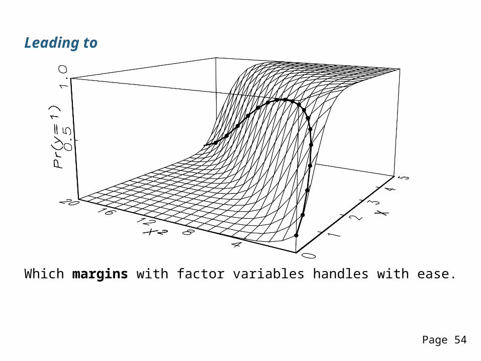
Leading to

Which margins with factor variables handles with ease.

Page 40

Modeling the effect of height and weight on arthritislogit arthritis c.age i.female i.ed3cat height weight

The question

Does height "by itself" increase the probability of arthritis?

The problem

1. Height and weight are linked.

2. Increasing height, holding weight constant is not the question.

3. Allow height to increase and let weight increase a corresponding amount.

o The type of problem has many applications.

Page 41

Estimate the model. sysuse svyhrs3, clear. svyset secu [pweight=kwgtr], strata(stratum) ///> vce(linearized) singleunit(missing). svy: logit arthritis c.age i.female i.ed3cat height weight. estimates store lgt

Predict weight from height. svy: reg weight height. local a = _b[_con]. local b = _b[height]

Compute std. dev. of height. svy: mean height. estat sd. local sd = el(r(sd),1,1). estimates restore lgt

Page 42

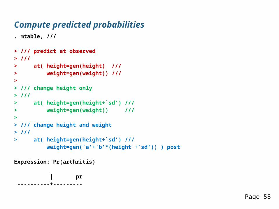
Compute predicted probabilities. mtable, ///

> /// predict at observed> ///> at( height=gen(height) ///> weight=gen(weight)) ///>> /// change height only> ///> at( height=gen(height+`sd') ///> weight=gen(weight)) ///>> /// change height and weight> ///> at( height=gen(height+`sd') /// weight=gen(`a'+`b'*(height +`sd')) ) post

Expression: Pr(arthritis)

| pr ----------+--------- 1 | 0.570 2 | 0.538 3 | 0.589

Page 43

Discrete changes: mlincom

Instead of lincom _b[2._at] - _b[1._at]

. mlincom 2 - 1, rowname(height_only)

| lincom pvalue ll ul --------------+---------------------------------------- height_only | -0.031 0.000 -0.046 -0.017

. qui mlincom 3 - 1, rowname(and_weight) add

. mlincom 3 - 2, rowname(2nd_difference) add

| lincom pvalue ll ul --------------+---------------------------------------- height_only | -0.031 0.000 -0.046 -0.017 and_weight | 0.020 0.008 0.005 0.034 2nd_differnce | 0.051 0.000 0.046 0.056

Page 44

Table with global and local meansGlobal means. sysuse binlfp4, clear. logit lfp i.wc k5 k618 i.agecat i.hc lwg inc

. qui mtable, atmeans at(wc=0 k5=(0 1 2 3)) estname(NoCol)

. qui mtable, atmeans at(wc=1 k5=(0 1 2 3)) estname(College) ///> atvars(_none) right. mtable, atmeans dydx(wc) at(k5=(0 1 2 3)) estname(Diff) stats(est p) ///> atvars(_none) names(columns) right


. matrix k5wc_global = _mtab_displayed

Page 45

Local means. mtable, over(k5) at(wc=0) estname(NoCol) atmeans atvars(k5)

Expression: Pr(lfp)

| 1. 2. 3. 1. | wc k5 k618 agecat agecat hc ----------+------------------------------------------------------------ 1 | 0 0 1.28 .436 .269 .358 2 | 0 1 1.75 .212 .0169 .517 3 | 0 2 1.31 .0385 0 .538 4 | 0 3 1.33 0 0 1 5 | 1 0 1.28 .436 .269 .358 6 | 1 1 1.75 .212 .0169 .517 7 | 1 2 1.31 .0385 0 .538 8 | 1 3 1.33 0 0 1

| | lwg inc pr ----------+----------------------------- 1 | 1.11 20 0.583 2 | 1.03 20.8 0.337 3 | 1.18 17.6 0.154 4 | 1.08 46.1 0.017 5 | 1.11 20 0.757 6 | 1.03 20.8 0.530 7 | 1.18 17.6 0.288

Page 46

8 | 1.08 46.1 0.037. qui mtable, over(k5) at(wc=1) estname(College) atmeans atvars(_none) right. mtable, over(k5) dydx(wc) estname(Diff) atmeans stats(est p) ///> atvars(_none) names(columns) right


. matrix k5wc_localk5 = _mtab_displayed

Page 47

Comparing global and local means | Global | Local | Global - Local k5 | NoCol Col Diff | NoCol Col Diff | NoCol Col Diff------+---------------------+---------------------+--------------------- 0.00 | 0.60 0.77 0.17 | 0.58 0.76 0.17 | -0.02 -0.02 0.01 1.00 | 0.27 0.46 0.18 | 0.34 0.53 0.19 | 0.06 0.07 0.01 2.00 | 0.09 0.17 0.09 | 0.15 0.29 0.13 | 0.07 0.11 0.05 3.00 | 0.02 0.05 0.03 | 0.02 0.04 0.02 | -0.01 -0.01 -0.01

Page 48

Plots with global and local meansIf time permits...

Predictions with global means. sysuse binlfp4, clear. logit lfp k5 k618 i.agecat i.wc i.hc lwg inc, nolog

. mgen, at(inc=(0(10)100)) atmeans stub(global_) predlabel(Global means)

Variables computed by the command:

. margins , at(inc=(0(10)100)) atmeans

Variable Obs Unique Mean Min Max Label------------------------------------------------------------------------------global_pr 11 11 .3608011 .0768617 .7349035 Global meansglobal_ll 11 11 .2708139 -.0156624 .6641427 95% lower limitglobal_ul 11 11 .4507883 .1693859 .8056643 95% upper limitglobal_inc 11 11 50 0 100 Family income exclud...------------------------------------------------------------------------------

Page 49

Predictions with local means. gen inc10k = trunc(inc/10) // income in 10K categories. mtable, over(inc10k) atmeans stat(est ll ul)

Expression: Pr(lfp)

| 2. 3. 1. 1. | k5 k618 agecat agecat wc hc ----------+------------------------------------------------------------ 1 | .202 1.43 .303 .222 .121 .0808 2 | .261 1.29 .363 .215 .212 .312:::snip:::

| | lwg inc pr ll ul ----------+------------------------------------------------- 1 | .922 7.25 0.641 0.584 0.698 2 | 1.08 15.1 0.600 0.559 0.642:::snip:::

. matrix tab = r(table)

. matrix tab = tab[1...,8..11]

. matrix colnames tab = local_inc local_pr local_ll local_ul

. svmat tab, names(col)

. label var local_pr "Local means"

. label var local_ll "95% lower limit"

. label var local_ul "95% upper limit"

. label var local_inc "Family income excluding wife's"

Page 50

Comparing global and local predictions0

.25

.5.7

51

Pr(

In L

abor

For

ce)

0 20 40 60 80 100Family income excluding wife's

Global means Local means

Page 52

Beyond the parametersOrdinal models are very restrictive

SD D N

A

SA

01

Pro

babi

lity

0 20 40 60 80 100Age

Pr(Strongly agree) Pr(Disagree)Pr(Agree) Pr(Strongly disagree)Pr(Neutral)

lcda13lec-orm-anderson-ordinalmodel scott long 2013-04-27

Page 53

Party identification. use partyid01, clear. tab party5, miss

Party: |1StDem 2Dem |3Indep 4Rep | 5StRep | Freq. Percent Cum.------------+----------------------------------- 1_SD | 266 19.25 19.25 2_D | 427 30.90 50.14 3_I | 151 10.93 61.07 4_R | 369 26.70 87.77 5_SR | 169 12.23 100.00------------+----------------------------------- Total | 1,382 100.00

. nmlab party5 age income black female highschool college

party5 Party: 1StDem 2Dem 3Indep 4Rep 5StRepage Ageincome Income (Thousands of dollars)black Respondent is blackfemale Respondent is femalehighschool High school is highest degreecollege College is highest degree

Page 54

ologit of partyid. ologit party5 age10 income10 i.black i.female i.highschool i.college. listcoef, help

ologit (N=1382): Factor Change in Odds

Odds of: >m vs <=m (More Republican vs Less Republican)

---------------------------------------------------------------------- party5 | b z P>|z| e^b e^bStdX SDofX-------------+-------------------------------------------------------- age10 | -0.06359 -2.037 0.042 0.9384 0.8988 1.6783 income10 | 0.09611 4.792 0.000 1.1009 1.3060 2.7781 1.black | -1.47593 -9.824 0.000 0.2286 0.6014 0.3445 1.female | -0.15711 -1.584 0.113 0.8546 0.9244 0.50011.highschool | 0.29417 1.943 0.052 1.3420 1.1563 0.4937 1.college | 0.64204 3.543 0.000 1.9004 1.3250 0.4383---------------------------------------------------------------------- b = raw coefficient z = z-score for test of b=0 P>|z| = p-value for z-test e^b = exp(b) = factor change in odds for unit increase in X e^bStdX = exp(b*SD of X) = change in odds for SD increase in X SDofX = standard deviation of X

Page 55

Parallel regression assumption. brant

Brant Test of Parallel Regression Assumption

Variable | chi2 p>chi2 df-------------+-------------------------- All | 89.84 0.000 18-------------+-------------------------- age10 | 42.87 0.000 3 income10 | 2.11 0.550 3 1.black | 12.82 0.005 3 1.female | 6.54 0.088 31.highschool | 2.92 0.404 3 1.college | 12.24 0.007 3----------------------------------------

A significant test statistic provides evidence that the parallelregression assumption has been violated.

SUGGESTION 1. Results of tests should be clearly explained (like chibar2).

Page 56

AMEmchangedcplot age10 income10, ...

12345

1 2 3 45

SD change

SD change

age10

income10

-.06 -.04 -.02 0 .02 .04 .06Discrete Change in Outcome Probability

OLM: average marginal effects

Page 57

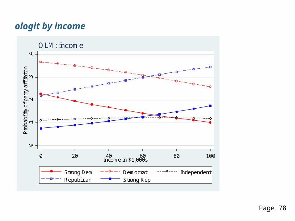
ologit by income0

.1.2

.3.4

Pro

babi

lity

of p

arty

affi

liatio

n

0 20 40 60 80 100Income in $1,000s

Strong Dem Democrat IndependentRepublican Strong Rep

OLM: income

Page 59

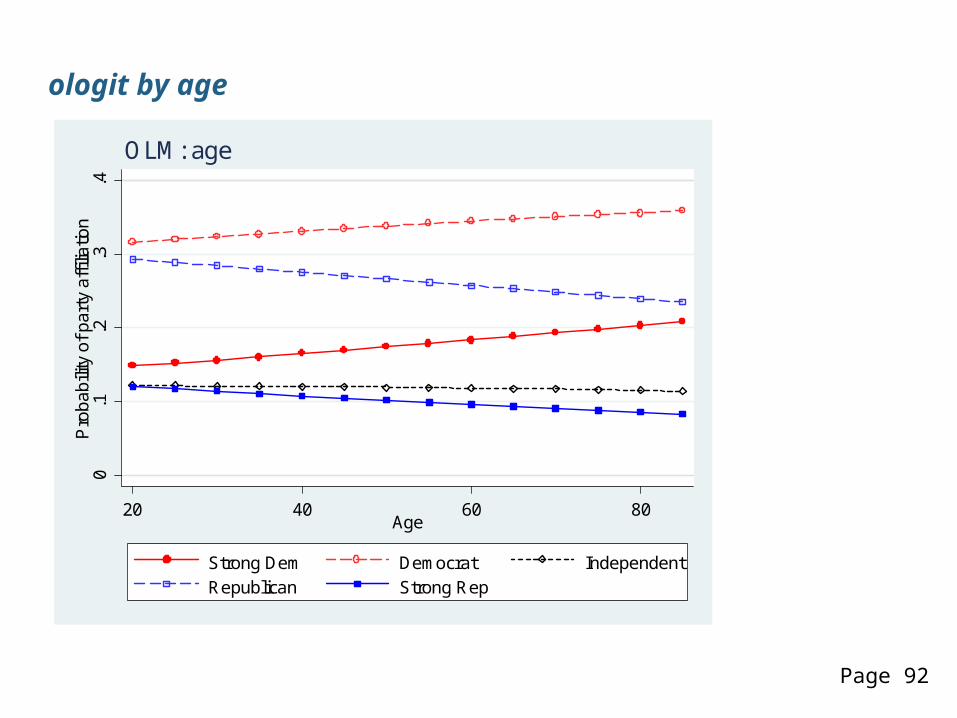
ologit by age0

.1.2

.3.4

Pro

babi

lity

of p

arty

affi

liatio

n

20 40 60 80Age


OLM: age

Page 60

mlogit of partyid. mlogit party5 age10 income10 i.black i.female i.highschool i.college::: snip :::

. mlogtest age10 income10, wald

Wald tests for independent variables (N=1382)

Ho: All coefficients associated with given variable(s) are 0

| chi2 df P>chi2-------------+------------------------- age10 | 43.815 4 0.000 income10 | 22.985 4 0.000---------------------------------------

Page 61

. listcoef age10 income10

mlogit (N=1382): Factor Change in the Odds of party5

Variable: age10 (sd=1.6783108)

Category 1 : Category 2 | b z P>|z| e^b e^bStdX--------------------------+---------------------------------------------1_SD : 2_D | 0.23617 4.761 0.000 1.2664 1.48641_SD : 3_I | 0.31618 4.781 0.000 1.3719 1.70001_SD : 4_R | 0.24533 4.576 0.000 1.2780 1.50941_SD : 5_SR | 0.02819 0.438 0.662 1.0286 1.04842_D : 1_SD | -0.23617 -4.761 0.000 0.7896 0.67282_D : 3_I | 0.08001 1.287 0.198 1.0833 1.1437:::snip:::5_SR : 4_R | 0.21714 3.594 0.000 1.2425 1.4397------------------------------------------------------------------------

Variable: income10 (sd=2.7781476):::

. mchange

. local min = log(.1)

. local max = log(3)

. local graphnm "`pgm'-partyid-mnlm-orplot"

. orplot, dc mcolors(`partycolor') min(`min') max(`max').

Page 62

mlogit odds ratio plot with ame'sorplot age10 income10, dc

12_

3_4_

5

1_2_

3_

45

SD change

SD change

age10

income10

0.50 0.71 1.00 1.41 2.00Odds Ratio Scale Relative to Category 2_D

-.69 -.35 0 .35 .69Logit Coefficient Scale Relative to Category 2_D

Page 63

mlogit AMEmchangedcplot age10 income10, std(ss) min(-.06) max(.06) gap(.02) ...

12 34 5

1 2 3 45

SD change

SD change

age10

income10

-.06 -.04 -.02 0 .02 .04 .06Discrete Change in Outcome Probability

MNLM: average marginal effects

Page 64

mlogit Probabilities to plot. mgen, atmeans at(`at_age') stub(mnlmage):::snip:::

. mgen, atmeans at(`at_inc') stub(mnlminc):::snip:::

Page 65

mlogit by income0

.1.2

.3.4

Pro

babi

lity

of p

arty

affi

liatio

n

0 20 40 60 80 100Income in $1,000s


#14 statcorp scott long 2013-08-03

MNLM: income

Page 66

ologit by income0

.1.2

.3.4

Pro

babi

lity

of p

arty

affi

liatio

n

0 20 40 60 80 100Income in $1,000s


OLM: income

Page 68

mlogit by age0

.1.2

.3.4

Pro

babi

lity

of p

arty

affi

liatio

n

20 40 60 80Age


MNLM: age

Page 70

ologit by age0

.1.2

.3.4

Pro

babi

lity

of p

arty

affi

liatio

n

20 40 60 80Age


OLM: age

Page 71

Post-estimation test & fitbrant: parallel regression test

mlogtest, wald or lr. mlogtest, lr

Likelihood-ratio tests for independent variables (N=337)

Ho: All coefficients associated with given variable(s) are 0

| chi2 df P>chi2-------------+------------------------- white | 8.095 4 0.088 ed | 156.937 4 0.000 exper | 8.561 4 0.073---------------------------------------

Why I'd like this included in the mlogit output...

Page 73

Base BlueCol: 0 significant coefficients e^b P>|z| WhiteCol: BlueCol 1.3978 0.720 Prof : BlueCol 1.7122 0.501 Craft : BlueCol 0.4657 0.227 Menial : BlueCol 0.2904 0.088

Base Craft: 1 significant coefficient e^b P>|z| BlueCol : Craft 2.1472 0.227 WhiteCol: Craft 3.0013 0.179 Prof : Craft 3.6765 0.044 Menial : Craft 0.6235 0.434

Base Menial: 1 significant coefficient e^b P>|z| Craft : Menial 1.6037 0.434 BlueCol : Menial 3.4436 0.088 WhiteCol: Menial 4.8133 0.082 Prof : Menial 5.8962 0.019

Page 74

Base Prof: 2 significant coefficients e^b P>|z| WhiteCol: Prof 0.8163 0.815 BlueCol : Prof 0.5840 0.501 Craft : Prof 0.2720 0.044 Menial : Prof 0.1696 0.019

Base WhiteCol: 0 significant coefficients e^b P>|z| ------------------+-------------------Prof : WhiteCol 1.2250 0.815 BlueCol : WhiteCol 0.7154 0.720 Craft : WhiteCol 0.3332 0.179 Menial : WhiteCol 0.2078 0.082

mlogtest, combineTesting if outcome categories are significantly differentiated.

mlogtest, iiaVarious not very useful but highly requested IIA tests.

Page 75

countfit: borrowed by SAS's countreg . countfit art fem mar kid5 phd ment, gen(cfeg) replace ///> inflate(fem mar kid5 phd ment) maxcount(6) ///

---------------------------------------------------------------------- Variable | Base_PRM Base_NBRM Base_ZIP ---------------------------------+------------------------------------art | Gender: 1=female 0=male | 0.799 0.805 0.811 | -4.11 -2.98 -3.30 Married: 1=yes 0=no | 1.168 1.162 1.109 | 2.53 1.83 1.46 Number of children < 6 | 0.831 0.838 0.866 | -4.61 -3.32 -3.02 PhD prestige | 1.013 1.015 0.994 | 0.49 0.42 -0.20 Article by mentor in last 3 yrs | 1.026 1.030 1.018 | 12.73 8.38 7.89 Constant | 1.356 1.292 1.898 | 2.96 1.85 5.28 ---------------------------------+------------------------------------lnalpha | Constant | 0.442 | -6.81

And so on for all models...Page 76

Comparison of Mean Observed and Predicted Count

Maximum At MeanModel Difference Value |Diff|---------------------------------------------PRM 0.091 0 0.026NBRM -0.015 3 0.006ZIP 0.054 1 0.015ZINB -0.019 3 0.008

PRM: Predicted and actual probabilities

Count Actual Predicted |Diff| Pearson------------------------------------------------0 0.301 0.209 0.091 36.4891 0.269 0.310 0.041 4.9622 0.195 0.242 0.048 8.5493 0.092 0.135 0.043 12.4834 0.073 0.061 0.012 2.1745 0.030 0.025 0.005 0.7606 0.019 0.010 0.009 6.8837 0.013 0.004 0.009 17.8158 0.001 0.002 0.001 0.3009 0.002 0.001 0.001 1.550------------------------------------------------Sum 0.993 0.999 0.259 91.964

And so on for all models summarized as a graph...

Page 77

-.1-.0

50

.05

.1O

bser

ved-

Pre

dict

ed

0 1 2 3 4 5 6 7 8 9Articles in last 3 yrs of PhD

PRM NBRMZIP ZINB

Note: positive deviations show underpredictions.

Page 78

Tests and Fit Statistics

PRM BIC= 3343.026 AIC= 3314.113 Prefer Over Evidence------------------------------------------------------------------------- vs NBRM BIC= 3169.649 dif= 173.377 NBRM PRM Very strong AIC= 3135.917 dif= 178.196 NBRM PRM LRX2= 180.196 prob= 0.000 NBRM PRM p=0.000------------------------------------------------------------------------- vs ZIP BIC= 3291.373 dif= 51.653 ZIP PRM Very strong AIC= 3233.546 dif= 80.567 ZIP PRM Vuong= 4.180 prob= 0.000 ZIP PRM p=0.000------------------------------------------------------------------------- vs ZINB BIC= 3188.628 dif= 154.398 ZINB PRM Very strong AIC= 3125.982 dif= 188.131 ZINB PRM-------------------------------------------------------------------------NBRM BIC= 3169.649 AIC= 3135.917 Prefer Over Evidence------------------------------------------------------------------------- vs ZIP BIC= 3291.373 dif= -121.724 NBRM ZIP Very strong AIC= 3233.546 dif= -97.629 NBRM ZIP------------------------------------------------------------------------- vs ZINB BIC= 3188.628 dif= -18.979 NBRM ZINB Very strong AIC= 3125.982 dif= 9.935 ZINB NBRM Vuong= 2.242 prob= 0.012 ZINB NBRM p=0.012-------------------------------------------------------------------------ZIP BIC= 3291.373 AIC= 3233.546 Prefer Over Evidence------------------------------------------------------------------------- vs ZINB BIC= 3188.628 dif= 102.745 ZINB ZIP Very strong AIC= 3125.982 dif= 107.564 ZINB ZIP LRX2= 109.564 prob= 0.000 ZINB ZIP p=0.000

Page 79

fitstatThese are generally not very useful, so don't waste time computing them.... fitstat

Measures of Fit for logit of lfp

Log-Lik Intercept Only: -514.873 Log-Lik Full Model: -452.724D(744): 905.447 LR(8): 124.299 Prob > LR: 0.000McFadden's R2: 0.121 McFadden's Adj R2: 0.103ML (Cox-Snell) R2: 0.152 Cragg-Uhler(Nagelkerke) R2: 0.204McKelvey & Zavoina's R2: 0.215 Efron's R2: 0.153Tjur's Discrimination Coef: 0.153 Variance of y*: 4.192 Variance of error: 3.290Count R2: 0.676 Adj Count R2: 0.249AIC: 923.447 AIC/N: 1.226BIC: 965.064 k: 9.000

Page 80

ic compare. logit lfp i.wc k5 k618 age i.hc lwg inc. fitstat, ic saving(nofv). logit lfp i.wc k5 k618 i.agecat i.hc lwg inc. fitstat, ic using(nofv) dif

Current nofv DifferenceModel: logit logitN: 753 753 0AIC 923.447 921.266 2.181AIC/N 1.226 1.223 0.003BIC 965.064 958.258 6.805k 9.000 8.000 1.000BIC (deviance) -4022.857 -4029.663 6.805BIC' -71.307 -78.112 6.805

Difference of 6.805 in BIC provides strong support for saved model.

SUGGESTION 1. A "lrtest" like command for use with IC measures.

Page 81

Listing coefficients. listcoef, help

zip (N=915): Factor Change in Expected Count

Observed SD: 1.926069

Count Equation: Factor Change in Expected Count for Those Not Always 0

---------------------------------------------------------------------- art | b z P>|z| e^b e^bStdX SDofX-------------+-------------------------------------------------------- fem | -0.20914 -3.299 0.001 0.8113 0.9010 0.4987 mar | 0.10375 1.459 0.145 1.1093 1.0503 0.4732 kid5 | -0.14332 -3.022 0.003 0.8665 0.8962 0.7649 phd | -0.00617 -0.199 0.842 0.9939 0.9939 0.9842 ment | 0.01810 7.886 0.000 1.0183 1.1872 9.4839---------------------------------------------------------------------- b = raw coefficient z = z-score for test of b=0 P>|z| = p-value for z-test e^b = exp(b) = factor change in expected count for unit increase in X e^bStdX = exp(b*SD of X) = change in expected count for SD increase in X SDofX = standard deviation of X

Page 82

Binary Equation: Factor Change in Odds of Always 0

---------------------------------------------------------------------- Always0 | b z P>|z| e^b e^bStdX SDofX-------------+-------------------------------------------------------- fem | 0.10975 0.392 0.695 1.1160 1.0563 0.4987 mar | -0.35401 -1.115 0.265 0.7019 0.8458 0.4732 kid5 | 0.21710 1.105 0.269 1.2425 1.1806 0.7649 phd | 0.00127 0.009 0.993 1.0013 1.0013 0.9842 ment | -0.13411 -2.964 0.003 0.8745 0.2803 9.4839---------------------------------------------------------------------- b = raw coefficient z = z-score for test of b=0 P>|z| = p-value for z-test e^b = exp(b) = factor change in odds for unit increase in X e^bStdX = exp(b*SD of X) = change in odds for SD increase in X SDofX = standard deviation of X

Page 83

Suggestionmargins related

1. More compact output.

2. Multiple outcomes in same estimation.

3. Save individual observations: margins, gen()4. Let predict predict everything that margins can estimate

5.margins, at(x=gen(x+sd(x)): egen() for at()6.marginsplot: save graphing variables and allow multiple outcomes

7.margins, autopost: automatically save current estimation command if it is in memory; if not in memory, load the one that was autoposted.

8. Better ways to incorporate local predictions: over(x=gen())?

Page 84

Data analysis1. A unified method for collecting results.

2. lrtest type command for ic

3. vuong function to compare models.

4.datasignature to detect all changes (controlled by save and use)

5. sem: LCA

Really useful that seem easy1.tab with variable name and variable label; values with value labels.

2.svy: means for fv's

3.reallyclearall4. fastcd by Nick Winter

Page 85

Programming1. Better tools for factor variables (or let Jeff make house calls)

o factor variables have greatly increased the barrier to user written commands.

2. r(table) for all commands with all key results (e.g., lincom)

3. Stronger controls for value labels

Graphics 1. 3d wireframe graphics

For workflow1. help mix not help me!

Move the best functions of SPost into Stata

Page 86

Thank you

Page 87

Contents

INTERPRETING REGRESSION MODELS.................................................................................................................1

WORKING WITH STATACORP..........................................................................................................................2

CONTINUING WORK...................................................................................................................................... 3

STATA AT INDIANA........................................................................................................................................4

GOALS FOR VISITING STATACORP.................................................................................................................... 5

Demo SPost13 wrappers for margins.................................................................................................5Other SPost13 commands.................................................................................................................. 5Things we'd like to see in Stata...........................................................................................................5

INTERPRETATION USING PREDICTIONS...............................................................................................................6

Interpreting nonlinear models............................................................................................................7Ways to use predictions......................................................................................................................7

THE TOOLS.................................................................................................................................................. 8

Official Stata........................................................................................................................................8SPost13 wrappers for margins and lincom.........................................................................................8Why not simply use margins and marginsplot?..................................................................................8

TABLES OF PREDICTIONS.................................................................................................................................9

Binary outcome...................................................................................................................................9

Page 88

Categorical outcomes....................................................................................................................... 14

MARGINAL EFFECTS.................................................................................................................................... 20

Marginal change............................................................................................................................... 21Discrete change................................................................................................................................ 21Binary outcome.................................................................................................................................22

Question.......................................................................................................................................22mchange with options (edited)....................................................................................................24

Ordinal outcomes............................................................................................................................. 27

WHAT LOGIT OUTPUT MIGHT LOOK LIKE..........................................................................................................32

AME AND MEM.......................................................................................................................................33

MEM................................................................................................................................................. 33AME.................................................................................................................................................. 33Should you replace one mean with another?...................................................................................33

DISTRIBUTION OF ME'S...............................................................................................................................34

Marginal change for income.............................................................................................................34Discrete change for woman attending college.................................................................................35

LINKED MARGINAL EFFECTS...........................................................................................................................37

Age and age-squared are strongly linked..........................................................................................38Leading to.................................................................................................................................... 39

Modeling the effect of height and weight on arthritis......................................................................40

Page 89

The question.................................................................................................................................40The problem.................................................................................................................................40Estimate the model......................................................................................................................41Predict weight from height..........................................................................................................41Compute std. dev. of height.........................................................................................................41

TABLE WITH GLOBAL AND LOCAL MEANS.........................................................................................................44

Global means....................................................................................................................................44Local means...................................................................................................................................... 45Comparing global and local means...................................................................................................47

PLOTS WITH GLOBAL AND LOCAL MEANS.........................................................................................................48

Predictions with global means..........................................................................................................48Predictions with local means............................................................................................................49Comparing global and local predictions............................................................................................50

BEYOND THE PARAMETERS........................................................................................................................... 51

Ordinal models are very restrictive...................................................................................................51Party identification........................................................................................................................... 52ologit of partyid................................................................................................................................ 53

Parallel regression assumption....................................................................................................54AME............................................................................................................................................. 55ologit by income...........................................................................................................................56ologit by age................................................................................................................................ 57

Page 90

mlogit of partyid............................................................................................................................... 58mlogit odds ratio plot with ame's................................................................................................60mlogit AME.................................................................................................................................. 61mlogit Probabilities to plot...........................................................................................................62mlogit by income..........................................................................................................................63ologit by income...........................................................................................................................64mlogit by age............................................................................................................................... 65ologit by age................................................................................................................................ 66

POST-ESTIMATION TEST & FIT.......................................................................................................................67

brant: parallel regression test...........................................................................................................67mlogtest, wald or lr...........................................................................................................................67mlogtest, combine............................................................................................................................69mlogtest, iia...................................................................................................................................... 69countfit: borrowed by SAS's countreg..............................................................................................70fitstat.................................................................................................................................................74ic compare........................................................................................................................................ 75Listing coefficients............................................................................................................................ 76

SUGGESTION..............................................................................................................................................78

margins related.................................................................................................................................78Data analysis..................................................................................................................................... 79Really useful that seem easy.............................................................................................................79Programming.................................................................................................................................... 80

Page 91

Graphics............................................................................................................................................80For workflow.....................................................................................................................................80Move the best functions of SPost into Stata.....................................................................................80

THANK YOU...............................................................................................................................................81

Page 92

interpreting regression models · web viewdraft: long-statacorp-2013-08-07.docx interpreting...

Documents