1

Department of Economics

1. Introduction

Econometrics Working Paper EWP1101

ISSN 1485-6441

Interpreting Dummy Variables in Semi-logarithmic Regression

Models: Exact Distributional Results

David E. Giles

Department of Economics, University of Victoria Victoria, B.C., Canada V8W 2Y2

January, 2011

Author Contact: David E. Giles, Dept. of Economics, University of Victoria, P.O. Box 1700, STN CSC, Victoria, B.C., Canada V8W 2Y2; e-mail: dgiles@uvic.ca; Phone: (250) 721-8540; FAX: (250) 721-6214

Abstract

Care must be taken when interpreting the coefficients of dummy variables in semi-logarithmic regression models. Existing results in the literature provide the best unbiased estimator of the percentage change in the dependent variable, implied by the coefficient of a dummy variable, and of the variance of this estimator. We extend these results by establishing the exact sampling distribution of an unbiased estimator of the implied percentage change. This distribution is non-normal, and is positively skewed in small samples. We discuss the construction of bootstrap confidence intervals for the implied percentage change, and illustrate our various results with two applications: one involving a wage equation, and one involving the construction of an hedonic price index for computer disk drives.

Keywords Semi-logarithmic regression, dummy variable, percentage change, confidence interval

JEL Classifications C13, C20, C52

2

1. Introduction

Semi-logarithmic regressions, in which the dependent variable is the natural logarithm of the

variable of interest, are widely used in empirical economics and other fields. It is quite common

for such models to include, as regressors, “dummy” (zero-one indicator) variables which signal

the possession (or absence) of qualitative attributes. Specifically, consider the following model:

l

i

m

jjjii DcXbaYln

1 1)( , (1)

where the iX ’s are continuous regressors and the jD ’s are dummy variables.

The interpretation of the estimated regression coefficients is straightforward in the case of the

continuous regressors in (1): 100 ib is the estimated percentage change in Y for a small change

in iX . However, as was pointed out initially by Halvorsen and Palmquist (1980), this

interpretation does not hold in the case of the estimated coefficients of the dummy variables. The

proper representation of the proportional impact, pj, of a zero-one dummy variable, Dj , on the

dependent variable, Y, is ]1)[exp( jj cp , and there is a well-established literature on the

appropriate estimation of this impact. More specifically, and assuming normal errors in (1),

Kennedy (1981) proposes the consistent (and almost unbiased)

estimator, 1))]ˆ(ˆ5.0exp(/)ˆ[exp(ˆ jjj cVcp , where jc is the OLS estimator of jc , and )ˆ(ˆjcV is

its estimated variance. Giles (1982) provides the formula for the exact minimum variance

unbiased estimator of jp , and Van Garderen and Shah (2002) provide the formulae for the

variance of the latter estimator, and the minimum variance unbiased estimator of this variance.

Derrick (1984) and Bryant and Wilhite (1989) also investigate this problem.

Surprisingly, this literature is often overlooked by some practitioners who interpret jc as if it

were the coefficient of a continuous regressor. However, there is a diverse group of empirical

applications that are more enlightened in this respect . Examples include the studies of Thornton

and Innes (1989), Rummery (1992), Levy and Miller (1996), MacDonald and Cavalluzzo (1996),

Lassibille (1998), Malpezzi et al. (1998) and Fedderson and Maennig (2009). There is general

agreement on the usefulness of jp (although see Krautmann and Ciecka, 2006 for an alternative

3

viewpoint). However, the literature is silent on the issue of the precise form of the finite-sample

distribution of this statistic. Such information is needed in order to conduct formal inferences

about jp . Asymptotically, of course, jp is the maximum likelihood estimator of jp , by

invariance, and so its limit distribution is normal, in general. As we will show, however,

appealing to this limit distribution can be extremely misleading even for quite large sample sizes.

In addition, Hendry and Santos (2005) show that jp will be inconsistent and asymptotically non-

normal for certain specific formulations of the dummy variable, so particular case must be taken

in such cases.

In the next section we provide more details about the underlying assumptions for the problem

under discussion and introduce some simplifying notation. Our main result, the density function

for jp , is derived in section 3, and in section 4 we present some numerical evaluations and

simulations that explore the characteristics of this density. Section 5 discusses the construction of

confidence intervals for jp based on jp , and two empirical applications are discussed in section

6. Section 7 concludes.

2. Assumptions and Notation

Consider the linear regression model (1) based on n observations on the data:

l

i

m

jjjii DcXbaY

1 1)ln( ,

(where the continuous regressors may also have been log-transformed, without affecting any of

the following discussion or results), and the random error term satisfies ),0(~ 2IN . Let jjd

be the jth diagonal element of 1)'( XX , where ),....,,,.....,,( 2121 ml DDDXXXX . In addition,

let jc be the OLS estimator of jc , so that ),(~ˆ 2jjjj dcNc . The usual unbiased estimator of the

variance of jc is

uddcV jjjjj )/(ˆ)ˆ(ˆ 22 ,

where )( mln , vee /)'(ˆ 2 , e is the OLS residual vector, and 2~ u .

Giles (1982) shows that the exact minimum variance estimator of pj is

4

1!

))ˆ(ˆ5.0(

)2/(

)2/()2/()ˆexp(~

0

i

ij

i

jj i

cV

icp

. (2)

He also shows that the approximation, jp , provided by Kennedy (1981) is extremely accurate

even in quite small samples. Van Garderen and Shah (2002) offer some further insights into the

accuracy of this approximation, and provide strong evidence that favours its use. They show that

jp~ may be expressed more compactly as

14/)ˆ(ˆ;)2/()ˆexp(~10 jjj cVFcp , (3)

where .);(.10 F is the confluent hypergeometric limit function (e.g., Abramowitz and Segun,

1965, Ch.15 ; Abadir, 1999, p.291). In addition, they derive the variance of jp~ , the exact

unbiased estimator of this variance, and a convenient approximation to this variance estimator as

is discussed in section 5 below.

Hereafter, and without loss of generality, we suppress the “j” subscripts to simplify the notation.

Our primary objective is to derive the density function of the following statistic, which estimates

the proportional impact of a dummy variable on the variable Y itself, in (1):

1))]ˆ(ˆ5.0exp(/)ˆ[exp(ˆ cVcp .

Note that 1ˆ p .

3. Main Result

First, consider the two random components of p , and their joint probability distribution.

Lemma 1: Let )ˆexp(cx , and ))ˆ(ˆ5.0exp( cVy . The joint probability p.d.f. of x and y is:

)}2/(][lnexp{)(ln"),( 2212/))/(1(1 2

dcxyyxkyxf d ,

where

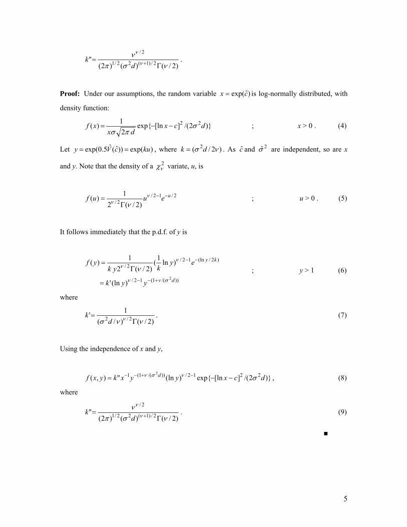
5

)2/()()2("

2/)1(22/1

2/

d

k .

Proof: Under our assumptions, the random variable )ˆexp(cx is log-normally distributed, with

density function:

)}2/(][lnexp{2

1)( 22 dcx

dxxf

; x > 0 . (4)

Let )exp())ˆ(ˆ5.0exp( kucVy , where )2/( 2 dk . As c and 2 are independent, so are x

and y. Note that the density of a 2 variate, u, is

2/12/2/ )2/(2

1)( ueuuf

; u > 0 . (5)

It follows immediately that the p.d.f. of y is

))/(1(12/

)2/(ln12/2/

2

)(ln'

)ln1

()2/(2

1)(

dv

ky

yyk

eykyk

yf

; y > 1 (6)

where

)2/()/(

1'

2/2

dk . (7)

Using the independence of x and y,

)}2/(][lnexp{)(ln"),( 2212/))/(1(1 2

dcxyyxkyxf d , (8)

where

)2/()()2("

2/)1(22/1

2/

d

k . (9)

■

6

We now have the joint p.d.f. of the two random components of p , and this can now be used to

derive the pd.f. of p itself.

Theorem 1: The exact finite-sample density function of p is

2/)1(24/)2(

2/2/

)(2)1ˆ()ˆ(

2

dp

evpf

))(;5.1,4/)2(())4/(

2)())(;5.0,)4/((

)4/)2((

1 211

211

FF ; 1ˆ p

where is the regression degrees of freedom, 2 is the regression error variance, d is the

diagonal element of the 1)'( XX matrix associated with the dummy variable in question, c is the

true value of the coefficient of that dummy variable, )2/(1 2d , cp )1ˆln( , and

.);.,(.11F is the confluent hypergeometric function (e.g., Gradzshteyn and Ryzhik, 1965,

p.1058).

Proof: Consider the change of variables from x and y to )(ln cxw and yyxp /)(ˆ . The

Jacobian of the transformation is 2)]1ˆ/()[exp( pcw , so

12/221)/( )]1ˆln()}[/()]()2/[(exp{)1ˆ(")ˆ,(2 pcwdcwwpkpwf dv ;

for cpwp )1ˆln(;1ˆ . (10)

The marginal density of p can then be obtained as

dwpcwdcwwpkpf d 12/221)/( )]1ˆln()}[/()]()2/[(exp{)1ˆ(")ˆ(2

,

(11)

where cp )1ˆln( .

Making the change of variable, )1ˆln( pcwz , we have

7

0

2212/1)/( )}/())]1ˆln((2/)[(exp{)1ˆ(")ˆ(2

dzdpzzzpkpf d . (12)

Then, defining )/(1 2d , (12) can be written as:

0

)()2/(12/]2/)1ˆln([1 22

)1ˆ(")ˆ( dzezepkpf zzpv . (13)

Then, using the integral result 3.462 (1) of Gradzshteyn and Ryzhik (1965, p.337),

))(()2/()1ˆ(")ˆ( 2/4/4/)(]2/)1ˆln([1 22

Deepkpf pv (14)

for 1ˆ p , where (.)D is the parabolic cylinder function (Gradzshteyn and Ryzhik, 1965,

p.1064). Using the relationship between the parabolic cylinder function and (Kummer’s)

confluent hypergeometric function, we have:

)2/)(;5.1,4/)2(())4/(

2)()2/)(;5.0,)4/((

)4/)2((

1

2))((

211

211

4/])([4/2/

2

FF

eD

(15)

where the confluent hypergeometric function is defined as (Gradzshteyn and Ryzhik, 1965,

p.1058):

............!3)2)(1(

)2)(1(

!2)1(

)1(1

!)(

)();,(

32

011

z

ccc

aaaz

cc

aaz

c

a

j

z

c

azcaF

j

j

j

j

(16)

Parenthetically, Pochhammer’s symbol is

1

0 )(

)()()(

j

kj

jk

, (17)

where it is understood that empty products in its construction are assigned the value unity. So,

recalling the definition of "k in (9), the density function of p can be written as:

8

2/)1(24/)2(

2/2/

)(2)1ˆ()ˆ(

2

dp

evpf (18)

))(;5.1,4/)2(())4/(

2)())(;5.0,)4/((

)4/)2((

1 211

211

FF ; 1ˆ p

■

4. Numerical Evaluations

Given its functional form, the numerical evaluation of the density function in (18) is non-trivial.

A helpful discussion of confluent hypergeometric (and related) functions is provided by Abadir

(1999), for example, and some associated computational issues are discussed by Nardin et al.

(1992) and Abad and Sesma (1996). In particular, it is well known that great care has to be taken

over the computation of the confluent hypergeometric functions, and the leading term in (18) also

poses challenges for even modest values of the degrees of freedom parameter, . Our evaluations

were undertaken using a FORTRAN 77 program, written by the author. This program

incorporates the double-precision complex code supplied by Nardin et al. (1989), to implement

the methods described by Nardin et al. (1992), for the confluent hypergeometric function; and the

GAMMLN routine from Press et al. (1992) for the (logarithm of the) gamma function. Monte

Carlo simulations were used to verify the exact numerical evaluations, and hence the validity of

(18) itself.

Figures 1 and 2 illustrate )ˆ( pf for small degrees of freedom and various choices of the other

parameters in the p.d.f.. The true value of p is 6.39 in Figure 1, and its values in Figure 2 are

2980.0 (c = 8) and 4446.1 (c = 8.4).

The quality of a normal asymptotic approximation to )ˆ( pf has been explored in a small Monte

Carlo simulation experiment, involving 5,000 replications, with code written for the SHAZAM

econometrics package (Whistler et al., 2004). The data-generating process used is

iiiii cDXbXbaY 2211)ln( ;

],0[...~ 2 Ndiii ; i = 1, 2, 3, …., n. (19)

9

Figure 1: p.d.f.'s of p-hat( v = 5, c = 2, d = 0.022)

0.00

0.05

0.10

0.15

0.20

0.25

0.30

0.35

0.40

-2.0 -1.0 0.0 1.0 2.0 3.0 4.0 5.0 6.0 7.0 8.0 9.0 10.0

p-hat

f(p

-ha

t)

sigma-squared = 100

sigma-squared = 50

Figure 2: p.d.f.'s of p-hat(v = 10, d = 1.5, sigma-squared = 2.4)

0.0E+00

5.0E-04

1.0E-03

1.5E-03

2.0E-03

2.5E-03

3.0E-03

3.5E-03

-4.0 0.0 4.0 8.0 12.0 16.0 20.0 24.0 28.0 32.0 36.0 40.0 44.0 48.0 52.0 56.0

p-hat

f(p

-hat

)

c = 8

c = 8.4

10

The regressors X1 and X2 were (pre-) generated as 21 and standard normal variables respectively,

and held fixed in repeated samples. We considered a range of sample sizes, n, to explore both the

finite-sample and asymptotic features of )ˆ( pf ; and we set a = 1, b1 = b2 = 0.1 c = 0.5, and

22 . The implied true value of p is 0.65, and the value of d is determined by the data for X,

the construction of the dummy variable, D, and the sample size, n, and two cases can be

considered. First, the number of non-zero values in D is allowed to grow at the same rate of n, so

the usual asymptotics apply. In this case we set D = 1 for i = 1, 2, …, )2/(n , and zero otherwise.

The sample 2R values for the fitted regressions are typical for cross-section data. Averaged over

the 5,000 replications, they are in the range 0.423 (n = 10) to 0.041 (n = 15,000). Second, the

number of the non-zero values in D is fixed at some value, Dn , in which case the usual

asymptotics do not apply. More specifically, in this second case the OLS estimator of c is

inconsistent, and its limit distribution is non-normal. This arises as a natural generalization of the

results in Hendry and Santos (2005), for the case where Dn = 1. In this second case we set Dn =

5, and assign only the last five values of D to unity, without loss of generality.

Table 1 reports summary statistics from this experiment, namely the %Bias of p , and the

standard deviation and skewness and kurtosis coefficients for its empirical sampling distribution.

All of the p-values associated with the Jarque-Bera (J-B) normality test are essentially zero,

except the one indicated. As we can see, for Case 1 (where standard asymptotics apply) the

consistency of p is reflected in the decline in the % biases and standard deviations as n

increases. For small samples, the distribution of p has positive skewness and excess kurtosis, as

expected from Figures 1 and 2. In Case 2 the usual asymptotics do not apply. The inconsistency

of p is obvious, as is the non-normality of its limit distribution. The latter is positively skewed

with large positive excess kurtosis. Figures 3 and 4 illustrate the sampling distributions of p

when n = 1,000, for Case 1 and Case 2 respectively in Table 1.

11

Table 1: Characteristics of Sampling Distribution for p

Case 1: )2/(nnD

n d %Bias( p ) S.D.( p ) Skew Excess Kurtosis

10 0.528 13.057 2.470 5.395 47.425

20 0.202 4.335 1.187 2.338 9.431

50 0.081 4.280 0.722 1.535 4.457

100 0.040 1.987 0.484 0.979 1.878

1000 0.004 0.696 0.149 0.165 -0.029

5000 0.001 0.177 0.065 0.156 0.197

15000 4103 0.045 0.037 0.070 0.034*

Case 2: 5Dn

n d %Bias( p ) S.D.( p ) Skew Excess Kurtosis

10 0.462 9.100 2.091 4.225 29.437

20 0.282 5.587 1.490 3.636 29.490

50 0.192 2.811 1.171 2.508 12.452

100 0.190 4.461 1.147 2.220 8.459

1000 0.168 -1.152 1.013 1.839 6.302

5000 0.167 -0.991 1.034 2.119 8.618

15000 0.167 -1.794 1.013 2.075 7.596

* J-B p-value = 0.115. J-B p-values for all other tabulated cases are zero, to at least 3 decimal places.

12

13

5. Confidence Intervals

For very large samples, p converges to the MLE of p, and the usual asymptotics apply. So,

inferences about p can be drawn by constructing standard (asymptotic) confidence intervals by

using the approximation )]ˆ(,0[)ˆ( pVNppnd , where

1)]ˆ([);2/())ˆ(exp()ˆ2exp()ˆ( 210 cVFcVcpV (20)

is derived by van Garderen and Shah (2002, p.151). They also show that the minimum variance

unbiased estimator of )ˆ( pV is

)ˆ(ˆ;)2/()ˆ(ˆ)4/(;)2/([)ˆ2exp()ˆ(ˆ

102

10 cVFcVFcpV . (21)

Here, )ˆ(ˆ cV is just the square of the standard error for c from the OLS regression results, and

.)(.;10 F is the confluent hypergeometric limit function defined in section 2. Van Garderen and

Shah (2002, p.152) suggest using the approximately unbiased estimator of )ˆ( pV , given by

))ˆ(ˆ2exp())ˆ(ˆexp()ˆ2exp()ˆ(~

cVcVcpV , (22)

and they note that in this context it is superior to the approximation based on the delta method.

So, using (22) and the asymptotic normality of p , large-sample confidence intervals are readily

constructed.

In small samples, however, the situation is considerably more complicated. Although p is

essentially unbiased (case 1), and a suitable estimator of its variance is available, Figures 1 and 2

and the results in Table 1 indicate that the sampling distribution of p is far from normal, even for

moderate sample sizes. The complexity of the density function for p in (18), and the associated

c.d.f., strongly suggest the use of the bootstrap to construct confidence intervals for p.

14

We have adapted the Monte Carlo experiment described in section 4 to provide a comparison of

the coverage properties of bootstrap percentile intervals and intervals based (wrongly) on the

normality assumption together with the variance estimator )ˆ(~

pV . We use 1,000 Monte Carlo

replications and 999 bootstrap samples – the latter number being justified by the results of Efron

(1987, p.181). In applying the bootstrap to the OLS regressions we use the “normalized residuals”

(Efron, 1979; Wu, 1986, p.1265). We limit our investigation to “Case 1” as far as the construction

of the dummy variable in model (19) is concerned, so that the usual asymptotics apply to c (and

hence p ).

The results appear in Table 2, where cL and cU are the lower and upper end-points of the 95%

confidence intervals. It will be recalled from Table 1 that the density for p is positively skewed.

So, in the case of the bootstrap confidence intervals the upper and lower end-points are taken as

the 0.025 and 0.975 percentiles of the bootstrap samples for p , averaged over the 999 such

samples. In the case of the normal approximation the limits are )ˆ(~

96.1ˆ pVp . In each case,

average values taken over the 1,000 Monte Carlo replications are reported in Table 2. A standard

bootstrap confidence interval has second-order accuracy. That is, if the intended coverage

probability is, say, α, then the coverage probability of the bootstrap confidence interval is

)( 1 nO . We also report the actual coverage probabilities (CP), and their associated standard

errors, for the intervals based on the normal approximation and )ˆ(~

pV . The confidence intervals

based on the normal approximation are always “shifted” downwards, relative to the bootstrap

intervals. The associated CP values are less than 0.95, but approach this nominal level as the

sample size increases. For sample sizes 100n the coverage probabilities of the approximate

intervals are within two standard errors of 0.95. Finally, we see that the constraint, p > -1, is

violated by the approximate intervals for 20n .

The simple bootstrap confidence intervals discussed here can, no doubt, be improved upon by

considering a variety of refinements to their construction, including those suggested in DiCiccio

and Efron (1996) and the associated published comments. However, we do not pursue this here.

15

Table 2: 95% Confidence Intervals for p

n Bootstrap Normal Approximation Using )ˆ(~

pV

cL cU cL cU CP (s.e.)

10 -0.800 21.436 -1.982 3.236 0.777 (0.059)

20 -0.515 4.769 -1.174 2.421 0.882 (0.021)

30 -0.436 3.622 -0.954 2.142 0.898 (0.015)

40 -0.306 3.059 -0.724 2.063 0.912 (0.012)

50 -0.270 2.719 -0.632 1.915 0.917 (0.011)

100 -0.055 1.883 -0.251 1.547 0.935 (0.008)

500 0.283 1.111 0.239 1.052 0.947 (0.007)

1000 0.384 0.968 0.362 0.939 0.948 (0.007)

5000 0.521 0.781 0.517 0.774 0.950 (0.007)

10000 0.559 0.743 0.557 0.740 0.950 (0.007)

15000 0.575 0.725 0.574 0.723 0.950 (0.007)

6. Applications

We consider two simple empirical applications to illustrate the various results discussed above.

The first application compares both the point and interval estimates of a dummy variable’s

percentage impact when these estimates are calculated in two ways: first, by naïvely interpreting

the coefficient in question as if it were associated with a continuous regressor; and second, using

the appropriate (and widely recommended) p100 , together with a bootstrap confidence interval.

The second application goes beyond the simple interpretation of the results of a semi-logarithmic

model with dummy variables, and shows how to construct an appropriate hedonic price index,

together with confidence intervals for each period’s index value that take account of the non-

standard density for p discussed in section 3. The effects of incorrectly using a normal

approximation are also illustrated.

16

6.1 Wage Determination Equation

Our first example involves the estimation of a simple wage determination equation. The data are

from the “CPS78” data-set provided by Berndt (1991). This data-set relates to 550 randomly

chosen employed people from the May 1978 current population survey, conducted by the U.S.

Department of Commerce. In particular, we focus on the sub-sample of 36 observations relating

to Hispanic workers. The following regression is estimated by OLS:

,

)(

654

3212

321

FEcSERVcSALESc

PROFcMANAGcUNIONcEXbEXbEDbaWAGEln (23)

where WAGE is average hourly earnings; ED is the number of years of education; and EX is the

number of years of labour market experience. The various zero-one dummy variables are: UNION

(if working in a union job); MANAG (if occupation is managerial/administrative); PROF (if

occupation is professional/technical); SALES (if occupation is sales worker); SERV (if occupation

is service worker); and FE (if worker is female).

The regression results, obtained using EViews 7.1 (Quantitative Micro Software, 2010), appear in

Table 3. The estimated coefficients have the anticipated signs and all of the regressors are

statistically significant at the 5% level. The various diagnostic tests support the model

specification. Importantly, the Jarque-Bera test supports the assumption that the errors in (23) are

normally distributed, as required for our analysis.

Table 4 reports estimated percentage impacts implied by the various dummy variables in the

regression. These have been calculated in two ways. First, we provide naïve estimates, based on

the incorrect (but frequently used) assumption that they are simply jc100 , where jc is the OLS

estimate of the jth dummy variable coefficient. Second, we report results based on the almost

unbiased estimator, jp100 . In each case, 95% confidence intervals are presented. The intervals

based on the naïve estimates are constructed using the standard errors reported in Table 3,

together with the Student-t critical values. The intervals based on the (almost) unbiased estimates

of the percentage impacts are bootstrapped, using 999 bootstrap samples.

17

Table 3: (Log-)Wage Determination Equations

(Hispanic Workers)

Const. 0.8342 (5.00) [0.00]

ED 0.0369 (2.69) [0.01]

EX 0.0267 (3.05) [0.00]

EX2 -0.0004 (-2.28) [0.02]

UNION 0.4551 (3.89) [0.00]

MANAG 0.3811 (2.89) [0.00]

PROF 0.4732 (4.93) [0.00]

SALES -0.4276 (-4.43) [0.00]

SERV -0.1512 (-1.82) [0.04]

FE -0.2791 (-3.66) [0.00]

n 36

2R 0.6388

J-B {p} 4.2747 {0.12}

RESET {p} 0.7263 {0.55}

BPG {p} 8.3423 {0.50}

White {p} 7.1866 {0.62}

Note: t-values appear in parentheses. These are based on White’s heteroskedasticity-consistent standard

errors. One-sided p-values appear in brackets. J-B denotes the Jarque-Bera test for normality of the errors;

RESET is Ramsey’s specification test (using second, third and fourth powers of the predicted values); BPG

and White are respectively the Breusch-Pagan-Godfrey and White nR2 tests for homoskedasticity of the

errors.

18

Table 4: Estimated Percentage Impacts of Dummy Variables

Dummy Variable Naïve ( jc100 ) Almost Unbiased ( jp100 )

UNION 45.51 56.56

[21.51 69.50] [28.52 91.81]

MANAG 38.11 45.12

[11.01 65.20] [-20.64 142.74]

PROF 47.32 59.79

[27.60 67.03] [18.15 112.03]

SALES -42.76 -35.09

[-62.60 -22.92] [-55.51 -7.45]

SERV -15.12 -14.33

[-32.19 1.95] [-29.12 4.32]

FE -27.91 -24.57

[-43.57 -12.25] [-36.06 -11.28]

Note: 95% confidence intervals appear in brackets. In the case of the almost unbiased percentage impacts,

the confidence intervals are based on a bootstrap simulation.

As expected from Table 1 of Halverson and Palmquist (1980), the percentage impacts in Table 4

are always algebraically larger when estimated appropriately than when estimated naïvely. These

differences can be substantial – for example, in the case of the PROF dummy variable the naïve

estimator understates the impact by 12.5 percentage points. In addition, the bootstrap confidence

intervals based on jp100 are wider than those based on jc100 in four of the six cases in Table

4. In the case of the MANAG dummy variable the respective interval widths are 163.4 and 54.2

percentage points. For the PROF dummy variable the corresponding widths are 93.9 and 39.4

percentage points. Except for the SERV and FE dummy variables, the naïve approach results in

confidence intervals that are misleadingly short.

19

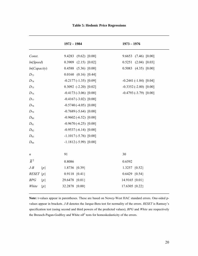
6.2 Hedonic Price Index for Disk Drives

As a second example, we consider regressions for computing hedonic price indices for computer

disk drives, as proposed by Cole et al. (1986). Their (corrected) data are provided by Berndt

(1991), and comprise a total of 91 observations over the years 1972 to 1984, for the U.S.. The

hedonic price regression is of the form:

84

7321 )()()(

jjj DcCapacitylnbSpeedlnbaPriceln , (24)

where Price is the list price of the disk drive; Speed is the reciprocal of the sum of average seek

time plus average rotation delay plus transfer rate; and Capacity is the disk capacity in

megabytes; and the dummy variables, Dj, are for the marketing years, 1973 to 1984. Some basic

OLS results, obtained using EViews 7.1, appear in Table 5. The associated hedonic price indices

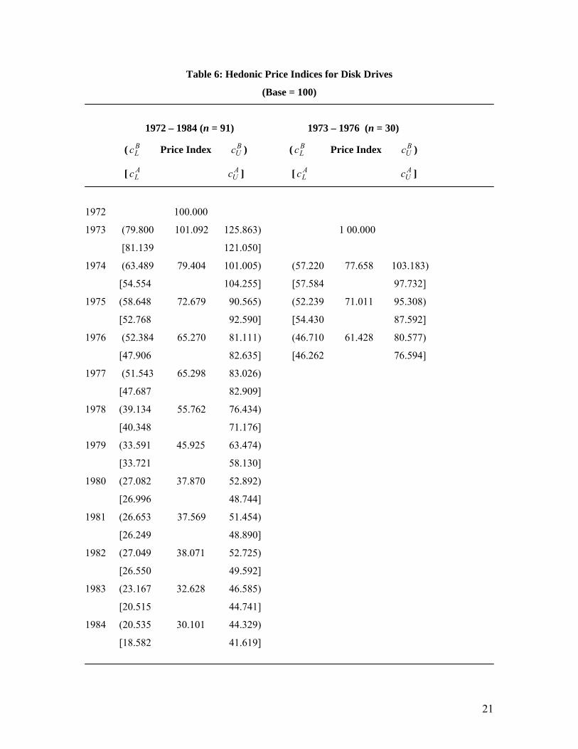
are presented in Table 6, with 95% confidence intervals.

Two sample periods are considered – the full sample of 91 observations, and a sub-sample of 30

observations. In each case, the Jarque-Bera test again supports the assumption that the errors in

(24) are normally distributed, as required for our various analytic results, and the RESET test

suggests that the functional forms of the regressions are well specified. Although there is some

evidence that the errors are heteroskedastic, we have compensated for this by reporting Newey-

West consistent standard errors. Two 95% confidence intervals are given for the price indices in

each year in Table 6. The end-points BLc and B

Uc relate to the bootstrap percentile intervals, based

on 999 bootstrap samples, for price index values based on p . The end-points for the approximate

confidence intervals, obtained using )ˆ(~

pV and a normal approximation for the sampling

distribution of p , are denoted ALc and A

Uc .

20

Table 5: Hedonic Price Regressions

1972 – 1984 1973 – 1976

Const. 9.4283 (9.62) [0.00] 9.6653 (7.46) [0.00]

ln(Speed) 0.3909 (2.15) [0.02] 0.5251 (2.04) [0.03]

ln(Capacity) 0.4588 (5.36) [0.00] 0.5083 (4.35) [0.00]

D73 0.0160 (0.16) [0.44]

D74 -0.2177 (-1.35) [0.09] -0.2441 (-1.84) [0.04]

D75 0.3092 (-2.20) [0.02] -0.3352 (-2.80) [0.00]

D76 -0.4173 (-3.06) [0.00] -0.4793 (-3.79) [0.00]

D77 -0.4167 (-3.02) [0.00]

D78 -0.5740 (-4.05) [0.00]

D79 -0.7689 (-5.64) [0.00]

D80 -0.9602 (-6.52) [0.00]

D81 -0.9670 (-6.25) [0.00]

D82 -0.9537 (-6.14) [0.00]

D83 -1.1017 (-5.76) [0.00]

D84 -1.1812 (-5.99) [0.00]

n 91 30

2R 0.8086 0.6592

J-B {p} 1.8736 {0.39} 1.3257 {0.52}

RESET {p} 0.9118 {0.41} 0.6429 {0.54}

BPG {p} 29.6478 {0.01} 14.9165 {0.01}

White {p} 32.2878 {0.00} 17.6305 {0.22}

Note: t-values appear in parentheses. These are based on Newey-West HAC standard errors. One-sided p-

values appear in brackets. J-B denotes the Jarque-Bera test for normality of the errors. RESET is Ramsey’s

specification test (using second and third powers of the predicted values); BPG and White are respectively

the Breusch-Pagan-Godfrey and White nR2 tests for homoskedasticity of the errors.

21

Table 6: Hedonic Price Indices for Disk Drives

(Base = 100)

1972 – 1984 (n = 91) 1973 – 1976 (n = 30)

( BLc Price Index B

Uc ) ( BLc Price Index B

Uc )

[ ALc A

Uc ] [ ALc A

Uc ]

1972 100.000

1973 (79.800 101.092 125.863) 1 00.000

[81.139 121.050]

1974 (63.489 79.404 101.005) (57.220 77.658 103.183)

[54.554 104.255] [57.584 97.732]

1975 (58.648 72.679 90.565) (52.239 71.011 95.308)

[52.768 92.590] [54.430 87.592]

1976 (52.384 65.270 81.111) (46.710 61.428 80.577)

[47.906 82.635] [46.262 76.594]

1977 (51.543 65.298 83.026)

[47.687 82.909]

1978 (39.134 55.762 76.434)

[40.348 71.176]

1979 (33.591 45.925 63.474)

[33.721 58.130]

1980 (27.082 37.870 52.892)

[26.996 48.744]

1981 (26.653 37.569 51.454)

[26.249 48.890]

1982 (27.049 38.071 52.725)

[26.550 49.592]

1983 (23.167 32.628 46.585)

[20.515 44.741]

1984 (20.535 30.101 44.329)

[18.582 41.619]

22

First, consider the results in Table 6 for the period 1973 to 1976. All of the approximate

confidence intervals are shorter (and misleadingly “more informative”) than those computed

using the bootstrap to mimic the true sampling distribution of p . For 1975, for example, the

approximate interval is of length 33.2, while the appropriate interval has length 43.1. The results

for the period 1972 to 1984 exhibit the same phenomenon in seven of the twelve years. These

results also demonstrate another unsettling feature of the approximate intervals. Consider the

values of the price index in 1973 and 1974. The appropriate 95% confidence interval for 1974,

namely (63.489 , 101.005), does not (quite) cover the point estimate of the index in 1973, namely

101.092. This suggests that the measured fall in the price index from 101.092 to 79.404 is

statistically significant at the 5% level. We reach the same conclusion by comparing the

appropriate confidence interval for 1973 with the point estimate of the index in 1974. In contrast,

we come to exactly the opposite conclusion if we make such comparisons using the approximate

confidence interval for 1974 and the point estimate for the index in 1973: the notional 21.45%

drop in prices from 1973 to 1974 is not statistically different from zero.

7. Conclusions

The correct interpretation of estimated coefficients of dummy variables in a semi-logarithmic

regression model has been discussed extensively in the literature. However, incorrect

interpretations are easy to find in empirical studies. We have explored this issue by extending the

established results in several respects. First, we have derived the exact finite-sample distribution

for Kennedy’s (1981) widely used (almost) unbiased estimator of the percentage impact of such a

dummy variable. This is found to be positively skewed for small samples, and non-normal even

for quite large sample sizes. Second, we have demonstrated the effectiveness of constructing

bootstrap confidence intervals for the percentage impact of interest, based on the correct

underlying distribution. Together, these contributions fill a gap in the known results for the

sampling properties of the correctly estimated percentage impact. Finally, two empirical

examples illustrate that with modest sample sizes, very misleading results can be obtained if the

dummy variables’ coefficients are not interpreted correctly; or if the non-standard distribution of

the implied percentage changes is ignored, and a normal approximation is blithely used instead.

Acknowledgement

I am very grateful to Ryan Godwin and Jacob Schwartz for several helpful discussions and for

their comments and suggestions.

23

References

Abad, J. and J. Sesma (1996). Computation of the regular confluent hypergeometric function.

Mathematica Journal, 5(4), 74-76.

Abadir, K. M. (1999). An introduction to hypergeometric functions for economists. Econometric

Reviews, 18, 287–330.

Abramowitz, M. and I. A. Segun, eds. (1965). Handbook of Mathematical Functions With

Formulas, Graphs, and Mathematical Tables, New York: Dover.

Berndt, E. R. (1991). The Practice of Econometrics: Classic and Contemporary, Reading, MA:

Addison-Wesley.

Bryant, R. and A. Wilhite (1989). Additional interpretations of dummy variables in

semilogarithmic equations. Atlantic Economic Journal, 17, 88.

Cole, R, Y. C. Chen, J. A. Barquin-Stollemann, E. Dulberger, N. Helvacian and J. H. Hodge

(1986). Quality-adjusted price indexes for computer processors and selected peripheral

equipment. Survey of Current Business, 66, 41-50.

Derrick, F. W. (1984). Interpretation of dummy variables in semilogarithmic equations: Small

sample implications. Southern Economic Journal, 50, 1185-1188.

DiCiccio, T. J. and B. Efron (1996). Bootstrap confidence intervals. Statistical Science, 11, 189-

228.

Efron, B. (1979). Bootstrap methods: Another look at the jackknife. Annals of Statistics, 7, 1-26.

Efron, B. (1987). Better bootstrap confidence intervals. Journal of the American Statistical

Association, 82, 171-185.

Fedderson, A. and W. Maennig (2009). Arenas versus multifunctional stadiums: which do

spectators prefer? Journal of Sports Economics, 10, 180-191.

Giles, D. E. A. (1982). The interpretation of dummy variables in semilogarithmic equations.

Economics Letters, 10, 77–79.

Gradshteyn, I. S., Ryzhik, I. W. (1965). Table of Integrals, Series, and Products (ed. A.

Jeffrey), 4th ed., New York: Academic Press.

Halvorsen, R. and R. Palmquist (1980). The interpretation of dummy variables in semilogarithmic

equations. American Economic Review, 70, 474–475.

Hendry, D. F. and C. Santos (2005), Regression models with data-based indicator variables.

Oxford Bulletin of Economics and Statistics, 67, 571-595.

Kennedy, P. E. (1981). Estimation with correctly interpreted dummy variables in semilogarithmic

equations. American Economic Review, 71, 801.

24

Krautmann, A. C. and J. Ciecka (2006). Interpreting the regression coefficient in semilogarithmic

functions: a note. Indian Journal of Economics and Business, 5, 121-125.

Lassibille, G. (1998). Wage gaps between the public and private sectors in Spain.

Economics of Education Review, 17, 83-92.

Levy, D. and T. Miller (1996). Hospital rate regulations, fee schedules, and workers’

compensation medical payments. Journal of Risk and Insurance, 63, 35-47.

Malpezzi, S., G. Chun, and R. Green (1998). New place-to-place housing price indexes for U.S.

metropolitan areas, and their determinants. Real Estate Economics, 26, 235-51.

MacDonald, J. and L. Cavalluzzo (1996). Railroad deregulation: pricing reforms, shipper

responses, and the effects on labor. Industrial and Labor Relations Review, 50, 80-91.

Nardin, M., W. F. Perger and A. Bhalla (1989). Algorithm 707: Solution to the confluent

hypergeometric function. FORTRAN 77 Source Code, Collected Algorithms of the

ACM, http://www.netlib.org/toms/707 .

Nardin, M., W. F. Perger and A. Bhalla (1992). Algorithm 707: Solution to the confluent

hypergeometric function. Transactions on Mathematical Software, 18, 345-349.

Press, W. H., S. A. Teukolsky, W. T. Vettering and B. P. Flannery (1992). Numerical Recipes in

FORTRAN: The Art of Scientific Computing, 2nd ed., New York: Cambridge University

Press.

Quantitative Micro Software (2010). EViews 7.1, Irvine, CA: Quantitative Micro Software.

Rummery, S. (1992). The contribution of intermittent labour force participation to the gender

wage differential. Economic Record, 68, 351-64.

Thornton, R. and J. Innes (1989). Interpreting semilogarithmic regression coefficients in labor

research. Journal of Labor Research, 10, 443-47.

Van Garderen, K. J. and C. Shah (2002). Exact interpretation of dummy variables in

semilogarithmic equations. Econometrics Journal, 5, 149-159.

Whistler, D., K. J. White, S. D. Wong and D. Bates (2004). SHAZAM Econometrics Software,

Version 10: User’s Reference Manual, Vancouver, B.C.: Northwest Econometrics.

Wu, C. F. J. (1986). Jackknife, bootstrap and other resampling methods in regression

analysis. Annals of Statistics, 14, 1261-1295.