interim report ir-01-070 us newsprint demand forecasts to...
TRANSCRIPT

International Institute forApplied Systems AnalysisSchlossplatz 1A-2361 Laxenburg, Austria
Tel: +43 2236 807 342Fax: +43 2236 71313
E-mail: [email protected]: www.iiasa.ac.at
Interim Reports on work of the International Institute for Applied Systems Analysis receive onlylimited review. Views or opinions expressed herein do not necessarily represent those of theInstitute, its National Member Organizations, or other organizations supporting the work.
Interim Report IR-01-070
US Newsprint Demand Forecasts to 2020Lauri Hetemäki ([email protected])Michael Obersteiner ([email protected]) and ([email protected])
Approved by
Sten NilssonLeader, Forestry Project
21 December 2001
ii
Contents
1 INTRODUCTION 1
2 BACKGROUND 2
3 EMPIRICAL MODELS 53.1 Classical Approach 5
3.2 Bayesian Model 6
3.3 Newspaper Circulation Model 8
4 THE DATA 10
5 EMPIRICAL RESULTS 115.1 Time Series Properties 11
5.2 Classical Model 13
5.3 Bayesian Model 18
5.4 Newspaper Circulation Model 19
5.5 Comparing the Forecasts 21
6 SUMMARY AND CONCLUSIONS 22
REFERENCES 24
APPENDIX I: THE BAYESIAN NORMAL-GAMMA REGRESSION MODEL 27
APPENDIX II: TIME SERIES PROPERTIES OF THE DATA 29
APPENDIX III: ESTIMATION RESULTS 37
iii
Abstract
The purpose of this study is to provide projections of newsprint demand for the UnitedStates (US) up to 2020. Three different approaches were used to compute theprojections. First, various specifications of the standard model used in forest productdemand literature, which we call the classical model, were estimated using annual datafrom 1971–2000. The results indicated that structural change in the newsprintconsumption pattern took place at the end of the 1980s. The classical model fails toexplain and forecast the structural change. It appears that changes related to thedevelopment of consumers’ preferences and information technology (IT) may havecaused the break down of the widely accepted positive relationship between the grossdomestic product (GDP) and newsprint demand. These observations motivated theformulation of alternative models. Thus, a Bayesian model that allows industry experts’prior knowledge about the future demand for newsprint to be included in the projectionswas estimated. Also, an ad hoc model, in which newsprint demand is a function ofchanges in newspaper circulation, was used to compute projections. Finally, theforecasts of these models are evaluated along with some of the existing projections.Besides providing an outlook for US newsprint demand, the study contributes to theexisting literature of long-term forest product demand by raising some methodologicalquestions and by applying new models to compute projections. Contrary to some recentprojections (e.g., FAO), the results indicate that US newsprint demand is likely todecline in the long run.

iv
Acknowledgments
The authors are grateful to the Finnish National Technology Agency (Tekes) forfinancially supporting this research.
We would like to sincerely thank Peter Ince for providing the information relating to theRPA projection.

v
About the Authors
While working on this paper, Lauri Hetemäki was a visiting senior research fellow atthe Fisher Center for the Strategic Use of Information Technology, University ofCalifornia, Berkeley, USA. His home institute is the Finnish Forest Research Institute(METLA), Finland. Michael Obersteiner is a research scholar in IIASA’s ForestryProject as well as at the Institute for Advanced Studies, Vienna, Austria.
1
US Newsprint Demand Forecasts to 2020Lauri Hetemäki and Michael Obersteiner
1 Introduction
The subject of newsprint demand has a long tradition in forest products literature.According to Buongiorno (1996), the first study using econometric methods to analyzeforest product markets was a study by Pringle (1954), in which he analyzed newsprintdemand in the United States (US). Since Pringle’s study, a large number of studies havebeen published on this topic. In addition, some organizations, such as the Food andAgriculture Organization of the United Nations (FAO) and the US Forest Service,regularly produces (roughly every 5 years) long-term forest products projections, whichalso include projections for US newsprint consumption. The purpose of theseprojections is, among others, to provide background information for policymakingconcerning the forest sector. The most recent FAO study was published in 1999 and theUS Forest Service study in 2001 (FAO, 1999a; Haynes, 2001).
The US newsprint market is particularly interesting to study due to its globalsignificance and the methodological challenges it raises. It is the world’s largestnewsprint market, being slightly larger than the whole European market, and consumingabout one third of the world’s total production of newsprint. Roughly about half of thisconsumption is based on imported newsprint (mainly from Canada). It is clear thatchanges in the US market will also have important implications to world newsprintmarkets. Furthermore, the US newsprint market turns out to be a challenging and topicalmarket to study from the methodological perspective. It appears that since the end of the1980s, structural change has taken place in newsprint consumption in the US, which theconventional forest products demand studies fail to explain and forecast. In particular,the historical relationship between newsprint consumption and economic activity (GDP)seems to have changed in recent years in the US. Therefore, there is also a need toreassess the performance of the models used to forecast newsprint demand.
In this study, the long-term US newsprint forecasts are computed using three differentmethods. First, various specifications of a model which has dominated forest productdemand literature for decades and which we name the “classical model” are estimated.In the classical model, the economic activity variable (GDP) and the price of newsprintare assumed to be the determinants of newsprint demand. Secondly, a Bayesianvariation of the classical model is estimated. This approach allows to include subjectiveprior information, such as industry experts’ views, to the estimation and forecasting ofnewsprint demand. To our knowledge, Bayesian methods have not yet been applied toforest economics literature in this way. However, as recent studies show, Bayesian

2
methods can be very useful for forecasting purposes and the approach has becomeincreasingly popular in applied econometrics (e.g., West and Harrison, 1997; Pole et al.,1999; Bauwens et al., 1999). The third method used is an ad hoc model, which includesthe changes in newspaper circulation as an explanatory variable, thus named as“newspaper circulation model”. Although, this model is not derived from economictheory (like the classical model), it can be justified on the basis of pragmatic reasoningand prior data analysis.
The results indicate that the sign of elasticity in newsprint demand with respect to GDPmay have turned from positive to negative. Moreover, the GDP parameter is no longerstatistically significant when a post-1987 sample is used for the estimation. Also, thenewsprint price variable does not appear to contain significant explanatory power, ifpost-1987 data is used. Finally, the overall conclusion from the various projections isthat the US newsprint demand is likely to decline in the next 20 years.
This paper is organized as follows. Section 2 provides the background for US newsprintdemand projections and discusses some of the existing studies; Section 3 presents thetheoretical and empirical methodology of the different approaches used in the presentstudy; Section 4 describes the data; Section 5 reports the empirical results; and finally inSection 6 some conclusions and general remarks are provided.
2 Background
The long-term projections of the future consumption of forest products have significantpractical relevance, since they are likely to influence government policymaking andprivate decision-making concerning the forest sector. Indeed, in the US the Forest andRangeland Renewable Resources Planning Act of 1974 (RPA) actually requires theSecretary of Agriculture to periodically conduct assessments of the nation’s renewableresources and their future development. In order to accomplish this objective, the USForest Service produces so-called RPA Timber Assessment studies, which also includelong-term projections for forest product consumption. These types of interests in the USand other countries sparked significant efforts in the late 1970s to build large scale andmore sophisticated models for forest products projections and forest policy analysis.The most well known outcomes of these efforts are the TAMM model (Adams andHaynes, 1980), the GTM model (Kallio et al., 1987), and the PELPS model (Zhang etal., 1993).1 These studies, along with the Solberg and Moiseyev (1997) study thatsurveys the European forest products modeling literature, give a good picture of thestate-of-the-art in long-term forest products forecasting.
FAO has been publishing long-term projections since the beginning of the 1960s, themost recent being the FAO (1999a) outlook study. This report, which is based on thePELPS model, provides projections for global forest products consumption, production,trade, and prices up to 2010.2 The most recent RPA Timber Assessment (Haynes, 2001)
1 For a discussion of the projections and the methods see, e.g., Buongiorno (1977; 1996), Baudin andBrooks (1995), and FAO (1999b).2 Although FAO (1999a, b) calls its projection model the Global Forest Products Model (GFPM), itsunderlying principles are the same as the PELPS model (Zhang et al., 1993).
3
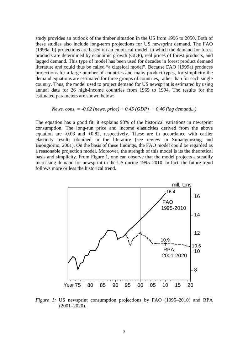
study provides an outlook of the timber situation in the US from 1996 to 2050. Both ofthese studies also include long-term projections for US newsprint demand. The FAO(1999a, b) projections are based on an empirical model, in which the demand for forestproducts are determined by economic growth (GDP), real prices of forest products, andlagged demand. This type of model has been used for decades in forest product demandliterature and could thus be called “a classical model”. Because FAO (1999a) producesprojections for a large number of countries and many product types, for simplicity thedemand equations are estimated for three groups of countries, rather than for each singlecountry. Thus, the model used to project demand for US newsprint is estimated by usingannual data for 26 high-income countries from 1965 to 1994. The results for theestimated parameters are shown below:
News. cons. = -0.02 (news. price) + 0.45 (GDP) + 0.46 (lag demandt-1)
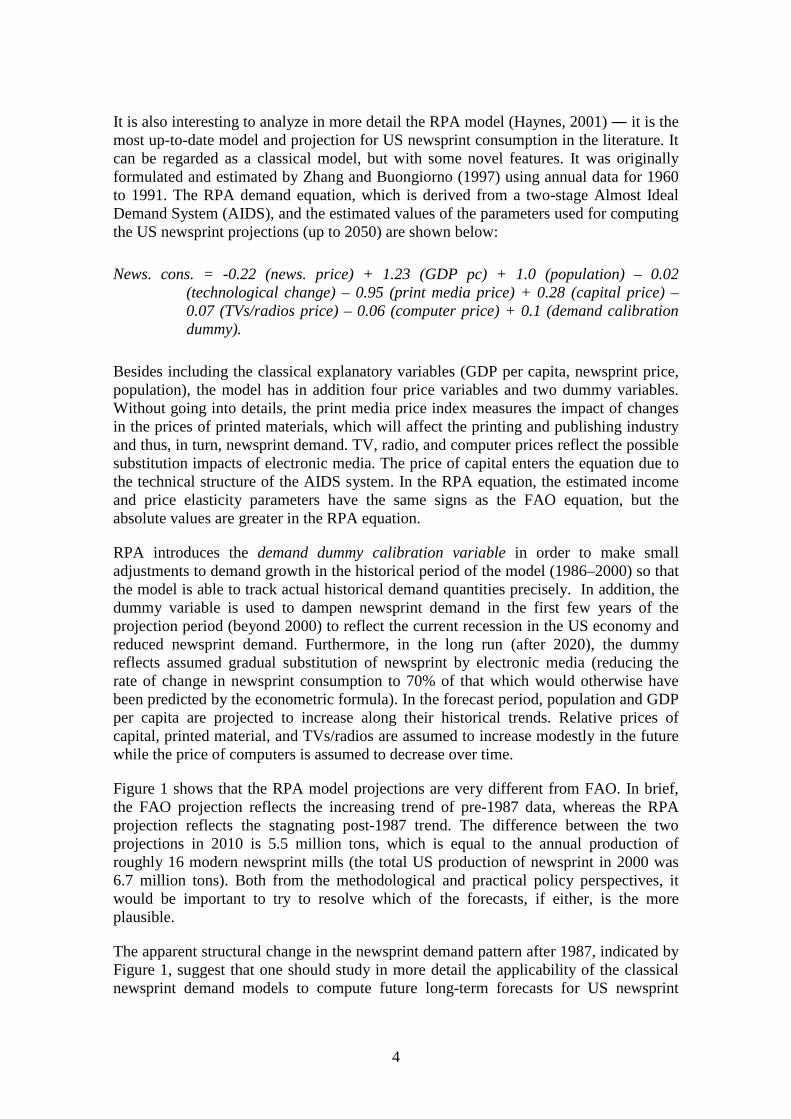
The equation has a good fit; it explains 98% of the historical variations in newsprintconsumption. The long-run price and income elasticities derived from the aboveequation are -0.03 and +0.82, respectively. These are in accordance with earlierelasticity results obtained in the literature (see review in Simangunsong andBuongiorno, 2001). On the basis of these findings, the FAO model could be regarded asa reasonable projection model. Moreover, the strength of this model is its the theoreticalbasis and simplicity. From Figure 1, one can observe that the model projects a steadilyincreasing demand for newsprint in the US during 1995–2010. In fact, the future trendfollows more or less the historical trend.
8
10
12
14
16
75 80 85 90 95 00 05 10 15 20
RPA
FAO1995-2010
2001-2020
mill. tons
Year
16.4
10.9I 10.6
Figure 1: US newsprint consumption projections by FAO (1995–2010) and RPA(2001–2020).
4
It is also interesting to analyze in more detail the RPA model (Haynes, 2001)― it is themost up-to-date model and projection for US newsprint consumption in the literature. Itcan be regarded as a classical model, but with some novel features. It was originallyformulated and estimated by Zhang and Buongiorno (1997) using annual data for 1960to 1991. The RPA demand equation, which is derived from a two-stage Almost IdealDemand System (AIDS), and the estimated values of the parameters used for computingthe US newsprint projections (up to 2050) are shown below:
News. cons. = -0.22 (news. price) + 1.23 (GDP pc) + 1.0 (population) – 0.02(technological change) – 0.95 (print media price) + 0.28 (capital price) –0.07 (TVs/radios price) – 0.06 (computer price) + 0.1 (demand calibrationdummy).
Besides including the classical explanatory variables (GDP per capita, newsprint price,population), the model has in addition four price variables and two dummy variables.Without going into details, the print media price index measures the impact of changesin the prices of printed materials, which will affect the printing and publishing industryand thus, in turn, newsprint demand. TV, radio, and computer prices reflect the possiblesubstitution impacts of electronic media. The price of capital enters the equation due tothe technical structure of the AIDS system. In the RPA equation, the estimated incomeand price elasticity parameters have the same signs as the FAO equation, but theabsolute values are greater in the RPA equation.
RPA introduces the demand dummy calibration variable in order to make smalladjustments to demand growth in the historical period of the model (1986–2000) so thatthe model is able to track actual historical demand quantities precisely. In addition, thedummy variable is used to dampen newsprint demand in the first few years of theprojection period (beyond 2000) to reflect the current recession in the US economy andreduced newsprint demand. Furthermore, in the long run (after 2020), the dummyreflects assumed gradual substitution of newsprint by electronic media (reducing therate of change in newsprint consumption to 70% of that which would otherwise havebeen predicted by the econometric formula). In the forecast period, population and GDPper capita are projected to increase along their historical trends. Relative prices ofcapital, printed material, and TVs/radios are assumed to increase modestly in the futurewhile the price of computers is assumed to decrease over time.
Figure 1 shows that the RPA model projections are very different from FAO. In brief,the FAO projection reflects the increasing trend of pre-1987 data, whereas the RPAprojection reflects the stagnating post-1987 trend. The difference between the twoprojections in 2010 is 5.5 million tons, which is equal to the annual production ofroughly 16 modern newsprint mills (the total US production of newsprint in 2000 was6.7 million tons). Both from the methodological and practical policy perspectives, itwould be important to try to resolve which of the forecasts, if either, is the moreplausible.
The apparent structural change in the newsprint demand pattern after 1987, indicated byFigure 1, suggest that one should study in more detail the applicability of the classicalnewsprint demand models to compute future long-term forecasts for US newsprint
5
consumption. The classical model implicitly assumes that the structure and behavior ofthe forest product markets remains the same as in the past. In particular, the projectionsare very sensitive to the assumptions concerning GDP growth. Besides the importanceof being able to accurately forecast the future GDP growth rate, it is important that therelationship between economic activity and demand for forest products remains stable.For the US, however, the relationship between newsprint consumption and GDP growthappears to have changed recently (see Section 5.1).
The RPA model acknowledges the recent structural changes and introduces dummyvariables and the impact of electronic media to try to capture these changes toprojections. The model implies that the relative prices between newsprint and electronicmedia are important determinants of newsprint demand. However, the underlyingstructure of the model is still the classical type, with GDP and the newsprint pricevariable playing an important role. Moreover, the dummy variables do not explain whythe structural changes have taken place.
In summary, the results from the literature and the data indicate that it is necessary toanalyze in more detail the apparent structural change in US newsprint demand, and theability of the conventional models to explain the more recent data. Also, there seems tobe a need to experiment with new types of models that would reflect the recent changesin consumers’ media behavior, and could be used for long-term forecasting purposes.
3 Empirical Models
In this Section, the empirical models used to project newsprint demand in the US from2001 to 2020 are presented. First, the “classical” model commonly used in foresteconomics literature is presented. Then the Bayesian approach is described, and finallythe so-called “newspaper circulation model” is outlined.
3.1 Classical Approach
The basic structure of the econometric models used to project forest products demandhas not changed significantly over time (see, e.g., McKillop, 1967; Kallio et al., 1987;Solberg and Moiseyev, 1997; Simangunsong and Buongiorno, 2001). Typically, thetheoretical background of the models is production theory, according to which the forestproduct enters as an intermediate input in the manufacturing production function alongwith other inputs. Assuming a behavioral hypothesis, e.g., cost minimization, allowsone to formulate an optimization problem from which the demand for the forest productcan be derived. Typically, this setting produces a demand function, such as the one inthe Global Forest Products Model (GFPM) (FAO, 1999a, b) and in Simangunsong andBuongiorno (2001), and expressed as equation (3.1):
ikikik,ik
a
ikikikik DXPaD ησσ1−= , (3.1)
where ikD is the demand in the ith country for commodity k, 1−D is demand in the
previous year, P is the price of the commodity, X is gross domestic product, and ηασ ,,
6
are the elasticities with respect to price, GDP, and past demand. For example, in thepresent case, i denotes the US and k denotes newsprint. The empirical modelcorresponding to equation (3.1), after logarithmic transformation and using theempirical data corresponding to the theoretical variables, can be written as:
ttnewstUSAtnewstnews dGDPpad εβββ ++++= − )ln()ln()ln()ln( 1,3,2,10, , (3.2)
where tnewsd , is the quantity of newsprint consumption in the US, tnewsp , is the real price
of newsprint, tUSAGDP , is the real gross domestic product in the US, 1, −tnewsd is a lagged
dependent variable measuring the possibility that in the short-run demand may adjustonly partially, tε is the error term, and t is a subscript denoting the time period. Since
the variables are in logarithmic form, the β -parameters can be interpreted directly aselasticities. Typically, the studies assume that the signs of the elasticities are known apriori. For example, Simangunsong and Buongiorno (2001:161) state that on the basisof the universality of economic laws of demand “one would expect the price elasticityof demand to be non-positive and the GDP elasticity to be non-negative”. In order toguarantee that the elasticities get correct signs and magnitudes, they can be restricted ordirected in empirical estimation to fulfill this objective. Indeed, in Simangunsong andBuongiorno (2001) the so-called Stein-rule shrinkage estimator is used for this purpose.
In the present study, various specifications of equation (3.2) are used to estimate thedemand for US newsprint demand and to compute long-term forecasts. However, in theestimation process, the signs or absolute values of the elasticities are not restricted.Also, the performance of the model is analyzed by estimating it for different datasamples, and by formally testing whether structural change has taken place.
3.2 Bayesian Model
The motivation for using the Bayesian model is the acknowledgement that besides thehistorical time series data, there can be other information that is helpful in making long-term projections. For example, forest industry experts may have reasonable and usefulviews about future forest products market developments. Through their experience andknowledge about the industry, technology, and markets experts may have informationthat can help to project future newsprint consumption patterns. Therefore, byincorporating subjective expert views, one may be able to improve on the informationset on which the “classical” projections are based. The Bayesian approach provides onepossible method to coherently incorporate this type of information into econometricforecasting models.
Bayesian methods have become increasingly popular in empirical applications in recentdecade (see, e.g., Bauwens et al., 1999; West and Harrison, 1997).3 Indeed, current theliterature is so large that one can identify many different methods within the Bayesianapproach. However, to our knowledge, the genuine Bayesian estimation with informed
3Important factors behind this popularity are the increasing computer capacity and availability of softwarepackages for Bayesian estimation.
7
priors has not been previously applied in forest products demand literature.4 A numberof Bayesian textbooks exist that explain the principles and differences of this approachrelative to the frequentist statistical methods (e.g., Pole et al., 1999; West and Harrison,1997). Here, only a brief description of one particular Bayesian method and themotivation of using it to forecast long-run newsprint demand in the US are given.
The starting point of our Bayesian framework is the above classical demand model.However, the Bayesian model allows the industry experts’ knowledge about therelationship between newsprint consumption and GDP growth to be incorporated in theestimation. For example, if the industry experts believe that GDP growth does not havean impact on newsprint demand in the future, one could reset the mean value of theprior distribution of GDP accordingly. Notationally, this can be expressed as movingfrom the classical model or pure model based prior )( 1−tt DGDPp to the Bayesian post-
intervention prior ),( 1 ttt IDGDPp − , where tI denotes the external information available
from the experts at time t. tI is called the prior information set and hereafter prior. The
prior of GDP is then combined with the information from observed data that isquantified probabilistically by the likelihood function. The resulting synthesis of priorand likelihood information is the posterior distribution of information. In other words,the posterior distribution quantifies the collection of the industry experts’ beliefs aboutthe GDP and the information gained from inference using historical data.
The Bayesian framework in the present study is also based on the classical equation[equation (3.2)] but, unlike the “frequentist approach”, the Bayesian model assumes aprior distribution for the GDP parameter ( 2β ). In this case, we used an informed prior
for the estimation of 2β , while all of the other parameters in equation (3.2) werederived using a so-called diffuse prior adding no additional information to the parameterestimation other than historical data.
Obviously, the choice of a particular prior distribution for the GDP parameter can havesubstantial impact on posterior model probabilities and the results. The technical detailson how the industry experts’ “informed prior information” is incorporated in ourBayesian econometric model is described in Appendix I. Here, we only present thegeneral idea.
The Bayesian parameters (posteriori) were estimated using the Normal-Gammaregression model. The Normal-Gamma model is a mixed distribution model where priorinformation is assumed to be distributed according to a gamma distribution, which iscombined with normally distributed parameters from time-series data. The estimationmethod used is ordinary least squares (OLS), as described in equations (A6) and (A7) inAppendix I. As prior information, we used information that was derived from USnewsprint consumption scenarios that three industry experts produced. Scenarios fornewsprint consumption were established by the industry experts up to 2013 in 5-yearintervals from 1998 onward. The methodology is briefly described in Section 4 and
4Simangunsong and Buongiorno (2001) use an “iterative empirical Bayesian estimator”, which isbasically a Stein-rule shrinkage estimator in the dynamic setting. The approach is qualitatively differentfrom the Bayesian method used here.
8
more detail is given in Obersteiner and Nilsson (2000). From the historical time seriesdata and the information provided by the experts, a panel data set was constructed andused to estimate equation 3.2. For the parameter estimation of the ‘expert model’ weused the OLS fixed effects estimator. Finally, for the computation of the Normal-Gamma regression model, the newsprint consumption data for the period 1987–2000was used.
3.3 Newspaper Circulation Model
The data on US newsprint consumption, GDP, and newsprint price indicate that thehistorical relationship between these variables appears to have changed after 1987 (seeSection 5 and Figure 4 for more details). Therefore, it is of interest to analyze whetherother variables exist that could explain the recent changes in the newsprint market andcontain important “causal” relationship to newsprint demand. Here, we experiment witha model that uses changes in newspaper circulation as an explanatory variable, whichwe therefore name “the newsprint circulation model”.
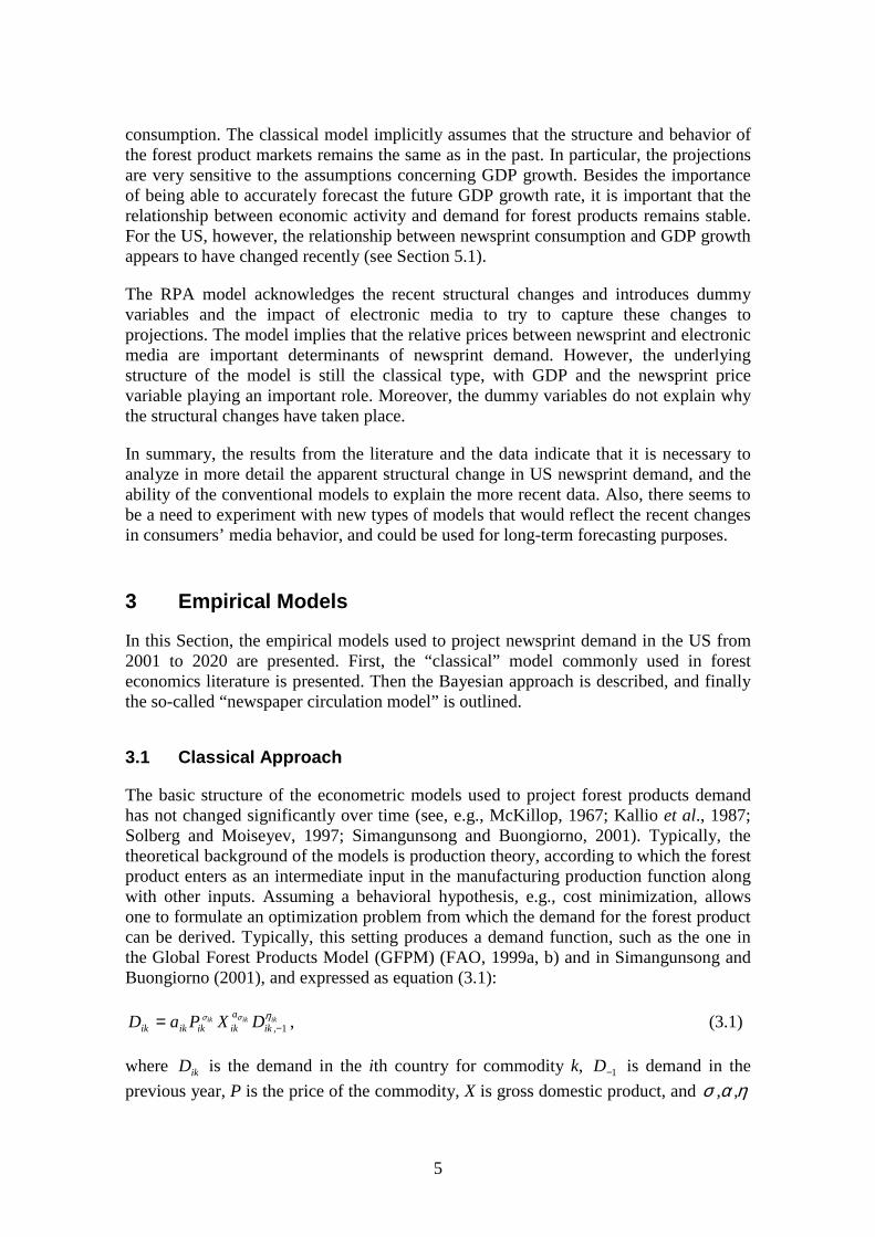
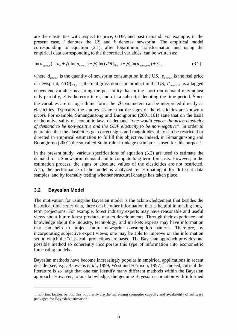
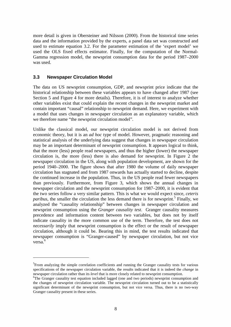
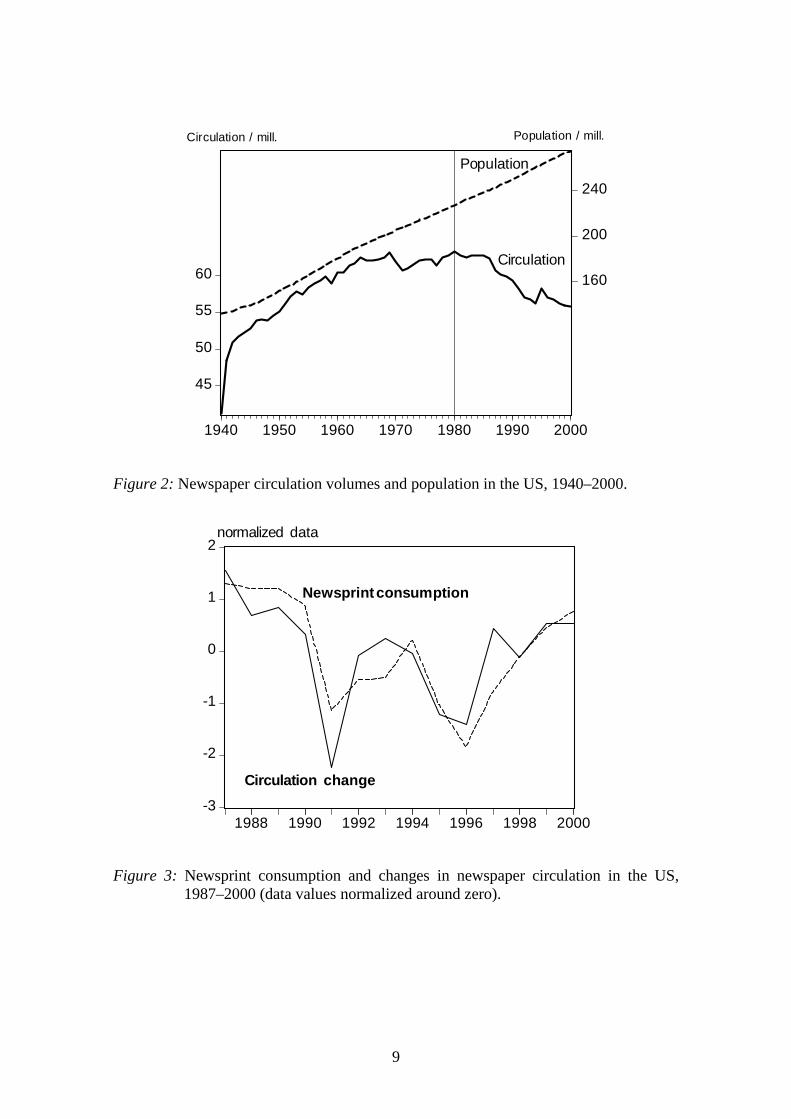
Unlike the classical model, our newsprint circulation model is not derived fromeconomic theory, but it is an ad hoc type of model. However, pragmatic reasoning andstatistical analysis of the underlying data suggest that changes in newspaper circulationmay be an important determinant of newsprint consumption. It appears logical to think,that the more (less) people read newspapers, and thus the higher (lower) the newspapercirculation is, the more (less) there is also demand for newsprint. In Figure 2 thenewspaper circulation in the US, along with population development, are shown for theperiod 1940–2000. The figure shows that after 1980 the volume of daily newspapercirculation has stagnated and from 1987 onwards has actually started to decline, despitethe continued increase in the population. Thus, in the US people read fewer newspapersthan previously. Furthermore, from Figure 3, which shows the annual changes innewspaper circulation and the newsprint consumption for 1987–2000, it is evident thatthe two series follow a very similar pattern. This is what we would expect since, ceterisparibus, the smaller the circulation the less demand there is for newsprint.5 Finally, weanalyzed the “causality relationship” between changes in newspaper circulation andnewsprint consumption using the Granger causality test. Granger causality measuresprecedence and information content between two variables, but does not by itselfindicate causality in the more common use of the term. Therefore, the test does notnecessarily imply that newsprint consumption is the effect or the result of newspapercirculation, although it could be. Bearing this in mind, the test results indicated thatnewspaper consumption is “Granger-caused” by newspaper circulation, but not viceversa.6
5From analyzing the simple correlation coefficients and running the Granger causality tests for variousspecifications of the newspaper circulation variable, the results indicated that it is indeed the change innewspaper circulation rather than its level that is more closely related to newsprint consumption.6The Granger causality test equation included lagged (one and two periods) newsprint consumption andthe changes of newsprint circulation variable. The newsprint circulation turned out to be a statisticallysignificant determinant of the newsprint consumption, but not vice versa. Thus, there is no two-wayGranger causality present in these series.
9
45
50
55
60 160
200
240
1940 1950 1960 1970 1980 1990 2000
Circulation
Population
Circulation / mill. Population / mill.
Figure 2: Newspaper circulation volumes and population in the US, 1940–2000.
-3
-2
-1
0
1
2
1988 1990 1992 1994 1996 1998 2000
Circulation change
Newsprintconsumption
normalized data
Figure 3: Newsprint consumption and changes in newspaper circulation in the US,1987–2000 (data values normalized around zero).
10
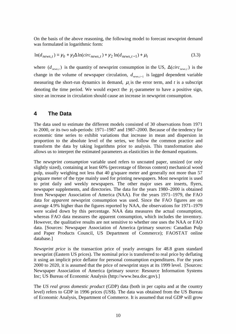
On the basis of the above reasoning, the following model to forecast newsprint demandwas formulated in logarithmic form:
ttnewstnewstnews dcircd µγγγ ++∆+= − )ln()ln()ln( 1,2,10, (3.3)
where )( ,tnewsd is the quantity of newsprint consumption in the US, )( ,tnewscirc∆ is the
change in the volume of newspaper circulation, 1, −tnewsd is lagged dependent variable
measuring the short-run dynamics in demand, tµ is the error term, and t is a subscript
denoting the time period. We would expect the 1γ -parameter to have a positive sign,since an increase in circulation should cause an increase in newsprint consumption.
4 The Data
The data used to estimate the different models consisted of 30 observations from 1971to 2000, or its two sub-periods: 1971–1987 and 1987–2000. Because of the tendency foreconomic time series to exhibit variations that increase in mean and dispersion inproportion to the absolute level of the series, we follow the common practice andtransform the data by taking logarithms prior to analysis. This transformation alsoallows us to interpret the estimated parameters as elasticities in the demand equations.
The newsprint consumption variable used refers to uncoated paper, unsized (or onlyslightly sized), containing at least 60% (percentage of fibrous content) mechanical woodpulp, usually weighing not less that 40 g/square meter and generally not more than 57g/square meter of the type mainly used for printing newspapers. Most newsprint is usedto print daily and weekly newspapers. The other major uses are inserts, flyers,newspaper supplements, and directories. The data for the years 1980–2000 is obtainedfrom Newspaper Association of America (NAA). For the years 1971–1979, the FAOdata for apparent newsprint consumption was used. Since the FAO figures are onaverage 4.9% higher than the figures reported by NAA, the observations for 1971–1979were scaled down by this percentage. NAA data measures the actual consumption,whereas FAO data measures the apparent consumption, which includes the inventory.However, the qualitative results are not sensitive to whether one uses the NAA or FAOdata. [Sources: Newspaper Association of America (primary sources: Canadian Pulpand Paper Products Council, US Department of Commerce); FAOSTAT onlinedatabase.]
Newsprint price is the transaction price of yearly averages for 48.8 gram standardnewsprint (Eastern US prices). The nominal price is transferred to real price by deflatingit using an implicit price deflator for personal consumption expenditures. For the years2000 to 2020, it is assumed that the price of newsprint stays at its 1999 level. [Sources:Newspaper Association of America (primary source: Resource Information SystemsInc; US Bureau of Economic Analysis (http://www.bea.doc.gov).]
The US real gross domestic product (GDP) data (both in per capita and at the countrylevel) refers to GDP in 1996 prices (US$). The data was obtained from the US Bureauof Economic Analysis, Department of Commerce. It is assumed that real GDP will grow

11
by 2.40% annually between 2001 and 2020. This is the same assumption that FAO(1999a) uses for its projections for the US from 1995 to 2010. The population data andprojections for 2020 refer to mid-year population and were obtained from the USCensus Bureau.
The US daily newspaper circulation refers to volume number in millions. [Source:Newspaper Association of America (http://www.naa.org/info/facts01/index.html).]
For the derivation of the Bayesian prior, the scenario plots constructed by a group ofresearch and development (R&D) managers of the paper industry were used. Theexperts participated in an online course on ‘Managing Technology for Value Delivery’at the University of British Columbia (Procter, 2000), in which scenarios for future USnewsprint demand were formulated. The expert group used a methodology for scenarioplotting developed by Obersteiner and Nilsson (2000). According to this methodology,course participants were asked to give quantitative input for about three main forcefactors determining the development of the US newsprint market. These force factorswere: (1) economic and life style development, (2) substitution of newspaper contentbetween paper and electronic media, and (3) newsprint intensity of newspaper making(basically future changes in the weight and size of the average newspaper). Thesefactors were allowed to vary for different population cohorts, distinguished by gender,age, and education, in order to model demographic shifts due to ageing and educationtriggered changes in the consumption pattern. Population trajectories were computed byIIASA’s Population Project (Lutz and Goujon, 2001) and were, thus, exogenousinformation to the experts. After the initial scenarios were formulated, they wereiteratively discussed, commented and improved by course participants.
There were only three experts that provided full scenarios during the course. It is clearthat the number of experts is very small, and therefore the results may not begeneralized to reflect the view of the whole industry, but rather represents a case study.However, from the Bayesian methodological point of view, the small number of expertsis not a critical issue for being able to use the method.
5 Empirical Results
5.1 Time Series Properties
Before the actual estimation of the different models, the time series properties of theunderlying data were analyzed using graphs, autocorrelation functions, AugmentedDickey-Fuller (ADF) and Philips-Perron (PP) tests, and various cointegration tests. Theresults indicated that newsprint consumption, GDP, and newsprint price series are non-stationary series (the results are shown in Appendix II).7 The various cointegration testresults pointed to the possibility of either zero or one cointegration relationship betweenthese variables. The newspaper circulation change series is on the border of being a I(0)
7The ADF tests were run both with and without the deterministic trend. According to the ADF test results,newsprint consumption, GDP, and price series can be regarded as I(1)-series at the 5% significance level.

12
or I(1) series ― the null hypothesis of non-stationarity can almost be rejected at the 5%level. The correlogram and the graph of the series suggest that it is a stationary series.
What implications should the above unit root and cointegration test results have tomodeling, estimation, and interpretation of the results? Clearly, when there are non-stationary variables in the models, particular concern should be attached to thepossibility of spurious regressions and biases in standard errors. However, from themodel strategy perspective, the results do not give unambiguous guidance. For example,in a recent survey, Allen and Fields (1999) conclude that the econometric literaturegives no generally accepted principles on how one should utilize the unit root andcointegration test results for model strategy. In the present study, this question is madeeven more difficult due to the small sample, which casts doubt as to the robustness ofunit root and cointegration tests, and also makes it difficult to estimate equations withlarge number of variables or systems models (in some specifications only 14observations were used, see below). In the present study, a strategy of trying to keep themodel specifications as simple as possible, given that the specifications were stillstatistically robust on basis of a number of different miss-specification tests, waschosen.
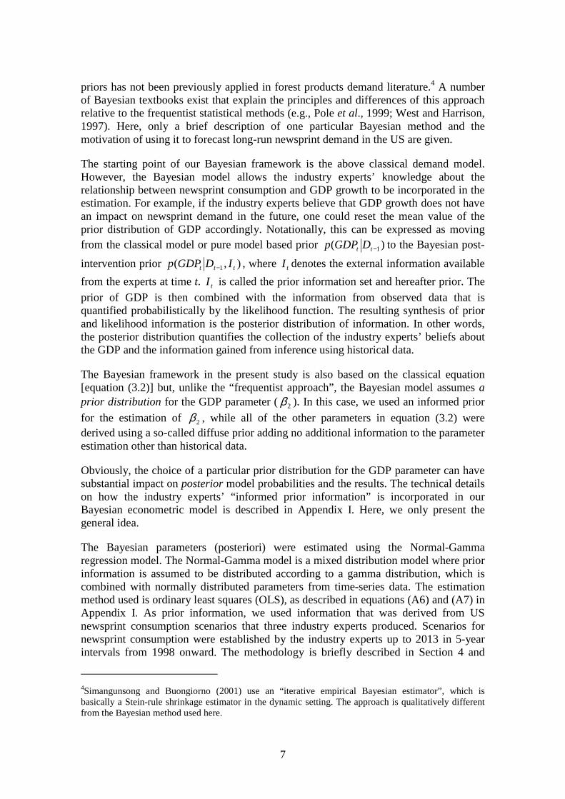
The initial analysis of the graphs and descriptive statistics of the data indicated that itwould be informative to estimate the models for various sample periods. Figure 4 showsthe newsprint consumption, real price, and real GDP series for the period 1971–2000(the series are in logarithms and normalized around 0). The trend in newsprintconsumption increased during 1971–1987, except for the periods relating to the oilcrises (1973–1975 and 1980–1982). After 1987, newsprint consumption started tostagnate, indicating a structural change in the pattern. Figure 4 also shows that thereason for stagnating newsprint consumption is probably not related to GDP ornewsprint price, since real GDP has continued to increase along its long-run trend andreal newsprint price has continued its declining trend.8 These changing patterns betweenthe series can also be observed in the simple correlation coefficients shown in Table 1.For the sample period, 1971–1987, the correlation coefficient between newsprintconsumption and real GDP is positive and very high (0.91), while for the period 1987–2000 it is negative and markedly lower (-0.25). Similarly, major changes in the signsand absolute values of the correlation coefficients between newsprint consumption andprice series, and between price series and GDP has taken place. However, wheninterpreting the latter correlation coefficients, one should be aware of the significantjump in the price series during 1995–1996.
In summary, the data analysis shows that the results are likely to be very sensitive to theparticular sample period used for the estimation. This suggests that one shouldexperiment with estimating the models for various time periods, instead of only usingthe whole sample period data.
8Also, the stagnation cannot be related to population growth, since it has also continued to increase alongthe long-run trend.

13
-3
-2
-1
0
1
2
1975 1980 1985 1990 1995 2000
GDP
Price
Newsprint
Normalized values
Year
Figure 4: US newsprint consumption, real GDP, and real newsprint price, 1971–2000.
Table 1: Correlation coefficients.
SAMPLE LGDP LPRICER
LNEWS 1971–20001971–19871987–2000
0.850.91-0.25
-0.48-0.090.29
LGDP 1971–20001971–19871987–2000
-0.650.27-0.59
5.2 Classical Model
Due to the structural break in the data, estimations of the classical model werecomputed for the following three periods: 1971–2000, 1971–1987, and 1987–2000. Thelatter two sub-periods have very few observations (17 and 14, respectively) and theresults should therefore be interpreted with caution. Still, the sub-period estimations arelikely to produce more meaningful results than using the whole sample. Besidesestimating the basic classical model for different observation periods, three differentmodel specifications were also estimated. Because of possible simultaneity between thenewsprint consumption and its price, a simple vector-autoregressive (VAR) systemsmodel was also estimated. Moreover, a static version of the classical model wascomputed. Finally, a specification where the impact of population changes wereincorporated by using the newsprint consumption per capita as an dependent variableand the GDP per capita as an explanatory variable was computed. Table 2 provides thesummary of the estimation results.
14
Table 2: Estimation results.
MODELestimatedperiod
Constantsr
GDPlr
GDPsr
Pricelr
PriceLaggedDemand
∆ Newsp.Circulat.
2_
R
B-G serialcorrelation
5% level
1. Classical1971–2000
-0.09(0.17)
0.08(1.05)
0.33 -0.01(0.17)
-0.05 0.77(6.09)
0.87 No
2. ClassicalVAR1971–2000
-0.35(0.70)
0.09(1.22)
0.09 0.05(0.80)
0.05 0.79(6.02)
0.87 No
3. Classical1971–1987
3.07(5.12)
0.70(6.57)
0.84 -0.49(4.79)
-0.58 0.16(1.18)
0.95 No
4. Classical1987–2000
0.93(0.80)
-0.01(0.07)
-0.01 -0.02(0.30)
-0.06 0.66(2.01)
0.17 No
5. ClassicalStatic1971–2000
-1.61(2.41)
0.44(7.18)
0.09(0.91)
0.72 Yes
6. ClassicalPer Capita1971–2000
0.68(0.71)
0.03(1.20)
0.13 -0.01(0.11)
-0.01 0.76(6.15)
0.87 No
7. BayesianPrior Panel1989–2013
1.10(2.30)
-0.06(2.22)
-0.54(5.09)
1.14(22.79)
0.98 No
8. BayesianPosterior1987–2000
0.92(0.46)
-0.02(0.10)
-0.04(0.24)
0.71(1.17)
No
9. NewspaperCirculation1987–2000
1.25(6.43)
0.51(6.47)
3.11(10.56)
0.92 No
Note: t-values are in parentheses.
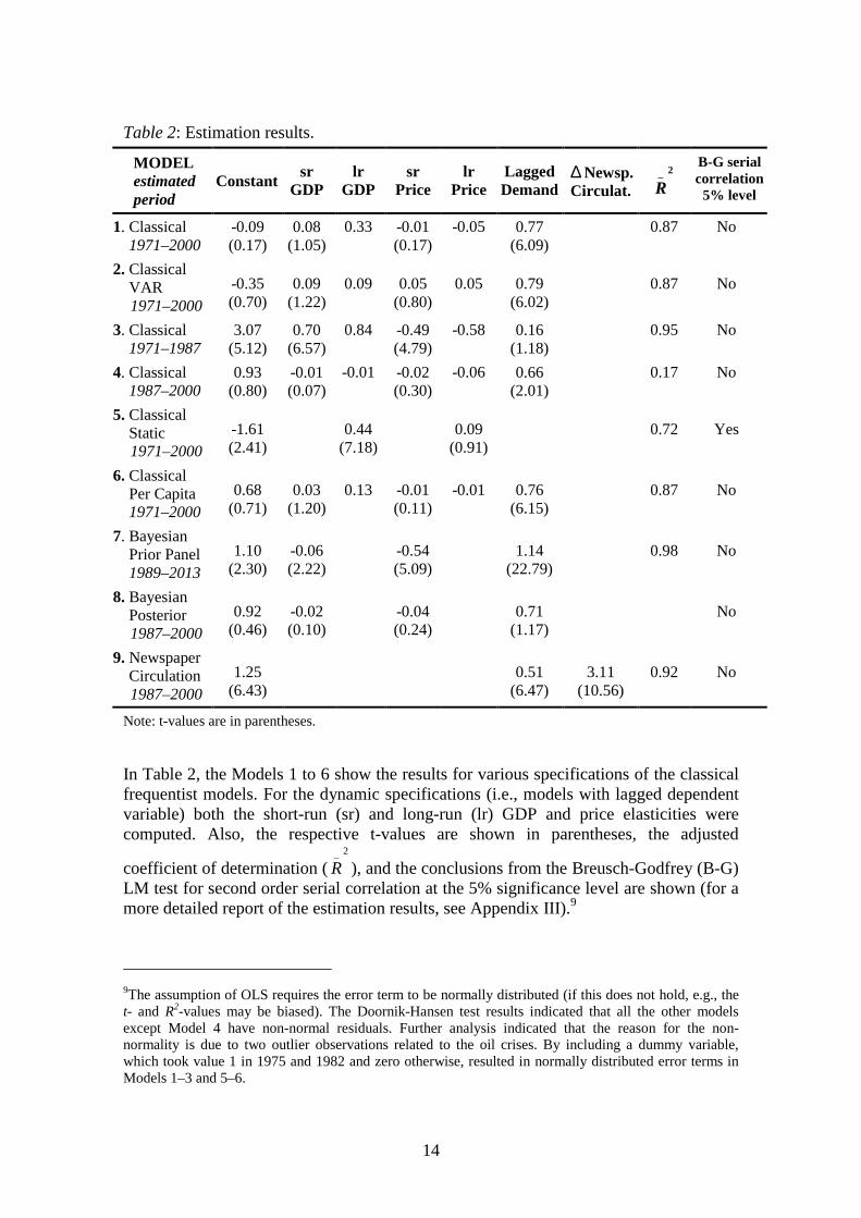
In Table 2, the Models 1 to 6 show the results for various specifications of the classicalfrequentist models. For the dynamic specifications (i.e., models with lagged dependentvariable) both the short-run (sr) and long-run (lr) GDP and price elasticities werecomputed. Also, the respective t-values are shown in parentheses, the adjusted
coefficient of determination (2_
R ), and the conclusions from the Breusch-Godfrey (B-G)LM test for second order serial correlation at the 5% significance level are shown (for amore detailed report of the estimation results, see Appendix III).9
9The assumption of OLS requires the error term to be normally distributed (if this does not hold, e.g., thet- and R2-values may be biased). The Doornik-Hansen test results indicated that all the other modelsexcept Model 4 have non-normal residuals. Further analysis indicated that the reason for the non-normality is due to two outlier observations related to the oil crises. By including a dummy variable,which took value 1 in 1975 and 1982 and zero otherwise, resulted in normally distributed error terms inModels 1–3 and 5–6.
15
In analyzing how well the different specifications succeed in explaining the historical
changes in newsprint consumption (2_
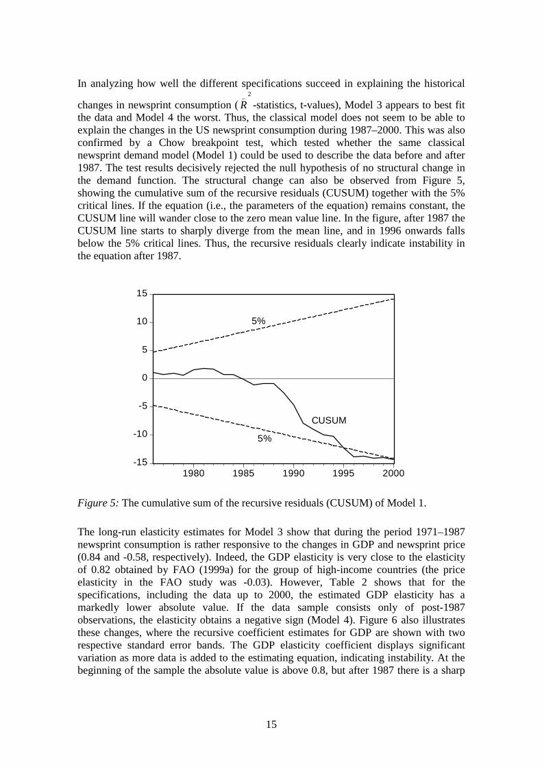
R -statistics, t-values), Model 3 appears to best fitthe data and Model 4 the worst. Thus, the classical model does not seem to be able toexplain the changes in the US newsprint consumption during 1987–2000. This was alsoconfirmed by a Chow breakpoint test, which tested whether the same classicalnewsprint demand model (Model 1) could be used to describe the data before and after1987. The test results decisively rejected the null hypothesis of no structural change inthe demand function. The structural change can also be observed from Figure 5,showing the cumulative sum of the recursive residuals (CUSUM) together with the 5%critical lines. If the equation (i.e., the parameters of the equation) remains constant, theCUSUM line will wander close to the zero mean value line. In the figure, after 1987 theCUSUM line starts to sharply diverge from the mean line, and in 1996 onwards fallsbelow the 5% critical lines. Thus, the recursive residuals clearly indicate instability inthe equation after 1987.
-15
-10
-5
0
5
10
15
1980 1985 1990 1995 2000
CUSUM
5%
5%
Figure 5: The cumulative sum of the recursive residuals (CUSUM) of Model 1.
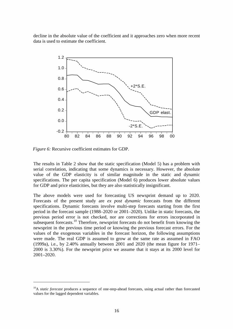
The long-run elasticity estimates for Model 3 show that during the period 1971–1987newsprint consumption is rather responsive to the changes in GDP and newsprint price(0.84 and -0.58, respectively). Indeed, the GDP elasticity is very close to the elasticityof 0.82 obtained by FAO (1999a) for the group of high-income countries (the priceelasticity in the FAO study was -0.03). However, Table 2 shows that for thespecifications, including the data up to 2000, the estimated GDP elasticity has amarkedly lower absolute value. If the data sample consists only of post-1987observations, the elasticity obtains a negative sign (Model 4). Figure 6 also illustratesthese changes, where the recursive coefficient estimates for GDP are shown with tworespective standard error bands. The GDP elasticity coefficient displays significantvariation as more data is added to the estimating equation, indicating instability. At thebeginning of the sample the absolute value is above 0.8, but after 1987 there is a sharp
16
decline in the absolute value of the coefficient and it approaches zero when more recentdata is used to estimate the coefficient.
-0.2
0.0
0.2
0.4
0.6
0.8
1.0
1.2
80 82 84 86 88 90 92 94 96 98 00
GDP elast.
+2*S.E.
-2*S.E.
Figure 6: Recursive coefficient estimates for GDP.
The results in Table 2 show that the static specification (Model 5) has a problem withserial correlation, indicating that some dynamics is necessary. However, the absolutevalue of the GDP elasticity is of similar magnitude in the static and dynamicspecifications. The per capita specification (Model 6) produces lower absolute valuesfor GDP and price elasticities, but they are also statistically insignificant.
The above models were used for forecasting US newsprint demand up to 2020.Forecasts of the present study are ex post dynamic forecasts from the differentspecifications. Dynamic forecasts involve multi-step forecasts starting from the firstperiod in the forecast sample (1988–2020 or 2001–2020). Unlike in static forecasts, theprevious period error is not checked, nor are corrections for errors incorporated insubsequent forecasts.10 Therefore, newsprint forecasts do not benefit from knowing thenewsprint in the previous time period or knowing the previous forecast errors. For thevalues of the exogenous variables in the forecast horizon, the following assumptionswere made. The real GDP is assumed to grow at the same rate as assumed in FAO(1999a), i.e., by 2.40% annually between 2001 and 2020 (the mean figure for 1971–2000 is 3.30%). For the newsprint price we assume that it stays at its 2000 level for2001–2020.
10A static forecast produces a sequence of one-step-ahead forecasts, using actual rather than forecastedvalues for the lagged dependent variables.
17
The forecast results for 2010 and 2020 are shown in Table 3. First, the FAO (1999a) andRPA (Haynes, 2001) projections are shown.11 FAO’s projection is based on estimating aclassical newsprint demand equation using data up to 1994 and making forecasts from1995 to 2010. Model 3 is estimated using data from 1971–1987 and forecasts are for theperiod 1988–2020. All the other specifications provide forecasts from 2001 to 2020(RPA actually provides projections up to 2050).
Table 3: Forecasts for US newsprint consumption (in millions metric tons).
MODEL 1994 2000 2010 2020
Actual values 11.9 12.2FAO (1999a) 13.5 16.4RPA (Haynes, 2001) 10.9 10.6
1. Classical 1971–2000 13.9 15.12. Classical VAR 1971–2000 13.3 14.33. Classical 1971–1987 18.0 21.8 26.8 32.74. Classical 1987–2000 11.9 11.85. Classical Static 1971–2000 14.4 15.96. Classical Per Capita 1971–2000 15.3 17.37. Bayesian Prior Panel 1989–2013 11.9 11.78. Bayesian Posterior 1987–2000 12.1 11.99. Newspaper Circulation 1987–2000 11.1 7.4
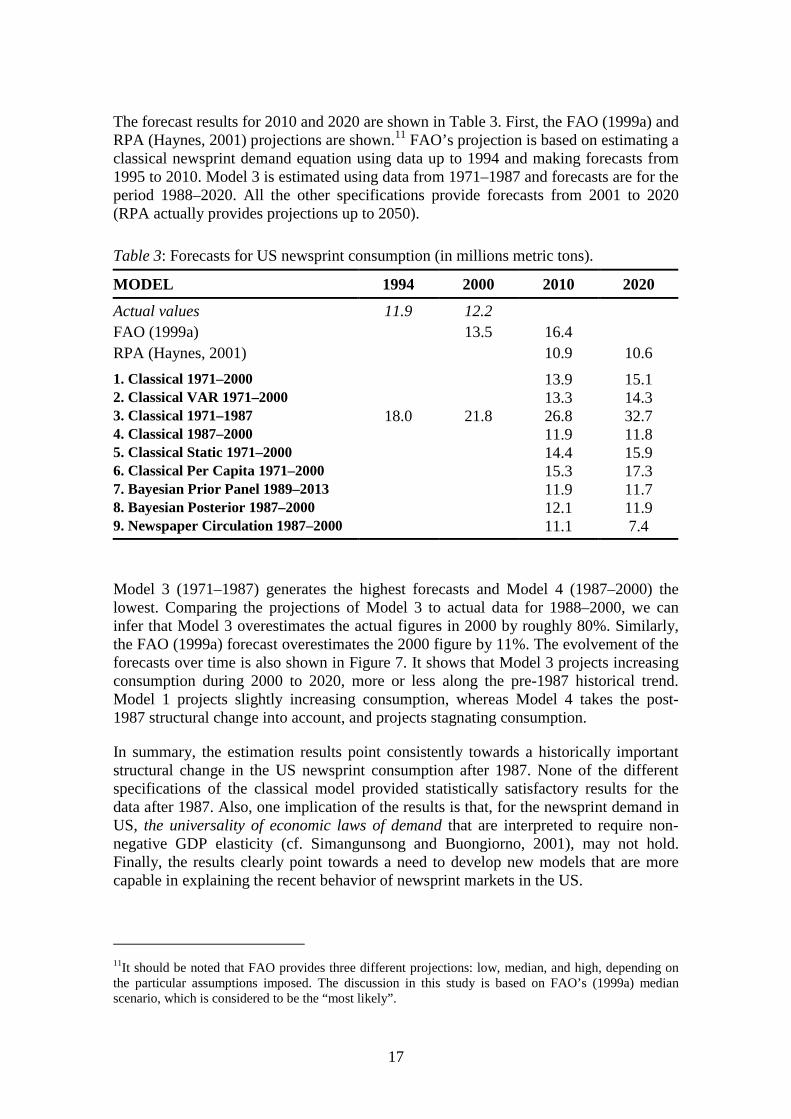
Model 3 (1971–1987) generates the highest forecasts and Model 4 (1987–2000) thelowest. Comparing the projections of Model 3 to actual data for 1988–2000, we caninfer that Model 3 overestimates the actual figures in 2000 by roughly 80%. Similarly,the FAO (1999a) forecast overestimates the 2000 figure by 11%. The evolvement of theforecasts over time is also shown in Figure 7. It shows that Model 3 projects increasingconsumption during 2000 to 2020, more or less along the pre-1987 historical trend.Model 1 projects slightly increasing consumption, whereas Model 4 takes the post-1987 structural change into account, and projects stagnating consumption.
In summary, the estimation results point consistently towards a historically importantstructural change in the US newsprint consumption after 1987. None of the differentspecifications of the classical model provided statistically satisfactory results for thedata after 1987. Also, one implication of the results is that, for the newsprint demand inUS, the universality of economic laws of demand that are interpreted to require non-negative GDP elasticity (cf. Simangunsong and Buongiorno, 2001), may not hold.Finally, the results clearly point towards a need to develop new models that are morecapable in explaining the recent behavior of newsprint markets in the US.
11It should be noted that FAO provides three different projections: low, median, and high, depending onthe particular assumptions imposed. The discussion in this study is based on FAO’s (1999a) medianscenario, which is considered to be the “most likely”.
18
8
12
16
20
24
28
32
36
00 02 04 06 08 10 12 14 16 18 20
Model 1
Model 3
Model 4
mill. tons
Year
Figure 7: Forecasts from classical models, 2001–2020.
5.3 Bayesian Model
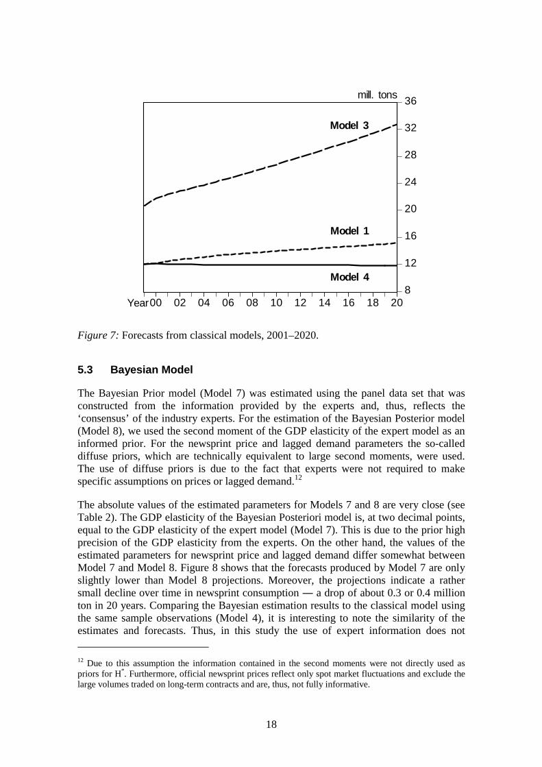
The Bayesian Prior model (Model 7) was estimated using the panel data set that wasconstructed from the information provided by the experts and, thus, reflects the‘consensus’ of the industry experts. For the estimation of the Bayesian Posterior model(Model 8), we used the second moment of the GDP elasticity of the expert model as aninformed prior. For the newsprint price and lagged demand parameters the so-calleddiffuse priors, which are technically equivalent to large second moments, were used.The use of diffuse priors is due to the fact that experts were not required to makespecific assumptions on prices or lagged demand.12
The absolute values of the estimated parameters for Models 7 and 8 are very close (seeTable 2). The GDP elasticity of the Bayesian Posteriori model is, at two decimal points,equal to the GDP elasticity of the expert model (Model 7). This is due to the prior highprecision of the GDP elasticity from the experts. On the other hand, the values of theestimated parameters for newsprint price and lagged demand differ somewhat betweenModel 7 and Model 8. Figure 8 shows that the forecasts produced by Model 7 are onlyslightly lower than Model 8 projections. Moreover, the projections indicate a rathersmall decline over time in newsprint consumption ― a drop of about 0.3 or 0.4 millionton in 20 years. Comparing the Bayesian estimation results to the classical model usingthe same sample observations (Model 4), it is interesting to note the similarity of theestimates and forecasts. Thus, in this study the use of expert information does not
12 Due to this assumption the information contained in the second moments were not directly used aspriors for H*. Furthermore, official newsprint prices reflect only spot market fluctuations and exclude thelarge volumes traded on long-term contracts and are, thus, not fully informative.
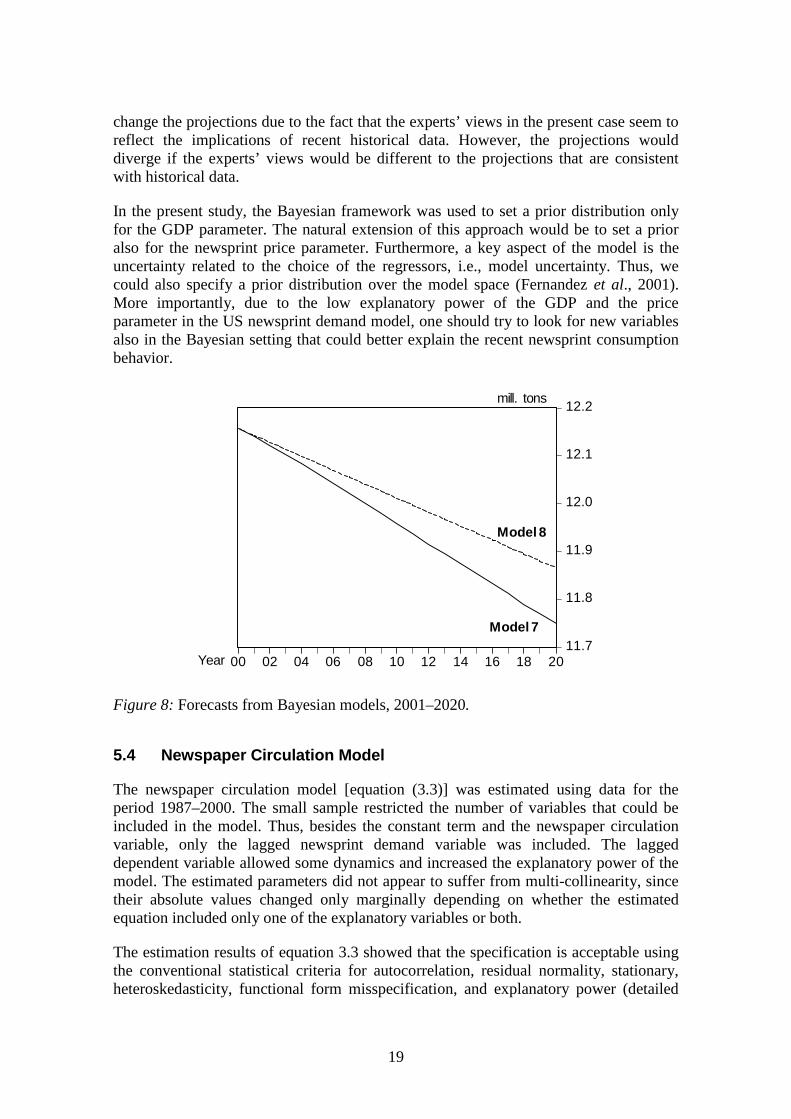
19
change the projections due to the fact that the experts’ views in the present case seem toreflect the implications of recent historical data. However, the projections woulddiverge if the experts’ views would be different to the projections that are consistentwith historical data.
In the present study, the Bayesian framework was used to set a prior distribution onlyfor the GDP parameter. The natural extension of this approach would be to set a prioralso for the newsprint price parameter. Furthermore, a key aspect of the model is theuncertainty related to the choice of the regressors, i.e., model uncertainty. Thus, wecould also specify a prior distribution over the model space (Fernandez et al., 2001).More importantly, due to the low explanatory power of the GDP and the priceparameter in the US newsprint demand model, one should try to look for new variablesalso in the Bayesian setting that could better explain the recent newsprint consumptionbehavior.
11.7
11.8
11.9
12.0
12.1
12.2
00 02 04 06 08 10 12 14 16 18 20
Model 8
Model 7
mill. tons
Year
Figure 8: Forecasts from Bayesian models, 2001–2020.
5.4 Newspaper Circulation Model
The newspaper circulation model [equation (3.3)] was estimated using data for theperiod 1987–2000. The small sample restricted the number of variables that could beincluded in the model. Thus, besides the constant term and the newspaper circulationvariable, only the lagged newsprint demand variable was included. The laggeddependent variable allowed some dynamics and increased the explanatory power of themodel. The estimated parameters did not appear to suffer from multi-collinearity, sincetheir absolute values changed only marginally depending on whether the estimatedequation included only one of the explanatory variables or both.
The estimation results of equation 3.3 showed that the specification is acceptable usingthe conventional statistical criteria for autocorrelation, residual normality, stationary,heteroskedasticity, functional form misspecification, and explanatory power (detailed
20
results shown in Appendix III). However, it should be borne in mind that the robustnessof these results are subject to the problems related to the small sample. The absolutevalue of the changes in newspaper circulation parameter indicates that, ceteris paribus,a 1% increase in newspaper circulation would lead to a 3.1% increase in newsprintdemand (see Table 2). Thus, newsprint demand appears to be very elastic with respectto circulation.
In order to be able to compute the conditional forecasts, assumptions about thedevelopment of newspaper circulation during 2001 to 2020 had to be made. These werebased on recent data on newspaper circulation and households “consumption” of media,and on the findings of some recent US media studies (e.g., NAA, 2001; UCLA, 2001).Looking at historical development from 1987 onwards, when newspaper circulationstarted to decline, we observe that circulation declined on average by 0.48% annuallyduring 1987–2000. However, the annual average rate of decline has acceleratedsomewhat, being 0.59% for the last five years. The declining interest in newspapers isapparent also in the data on media consumption of US households. Table 920 in theStatistical Abstracts of the United States (2000), shows how many hours householdsannually spend on different media. According to these statistics, households spent 10%less time reading newspapers in 2000 than in 1992, while at the same time increasingInternet consumption by 2050%. Although the relative change in Internet consumptionis huge, its absolute significance is small due to the very low starting level.Nevertheless, the underlying tendency is declining newspaper consumption andsimultaneous increase in Internet consumption. A similar pattern was found in a recentstudy by the North American Newspaper Association (NAA, 2001:4), which surveyedthe media behavior of a nationally representative sample of 4003 adults, aged 18 andover. According to the study “The first and perhaps most significant finding of the studyis the decline in penetration of traditional media including newspapers, TV, and radioand the concurrent rise in the use of the Internet as a source of news and information”.The study also reports evidence that the two phenomena are connected, i.e., theincreasing usage of the Internet accelerates the decline in newspaper readership. Thesefindings are supported by other studies, such as the NAA (2001) and UCLA (2001)survey studies.13
In the newspaper circulation model, the above data and surveys were interpreted toimply an increasing rate of decline in newspaper circulation in the US during 2001 to2020. In particular, we assumed that US newspaper circulation is declining by 1%annually during 2001–2005, by 2% annually during 2006–2010, by 4% annually during2011–2015, and by 8% annually during 2016–2020. These numbers are ad hoc, andshould not be taken as precise projections, but rather as one possible scenario fornewspaper circulation development. More important than the absolute numbers is thegeneral trend. The above numbers assume that no dramatic change is taking place andthat the rate of circulation decline increases steadily. We regard the assumptions to bemoderate rather than extreme.
13 It may be noted, that newsprint consumption is stagnating also in Japan and in some Europeancountries.
21
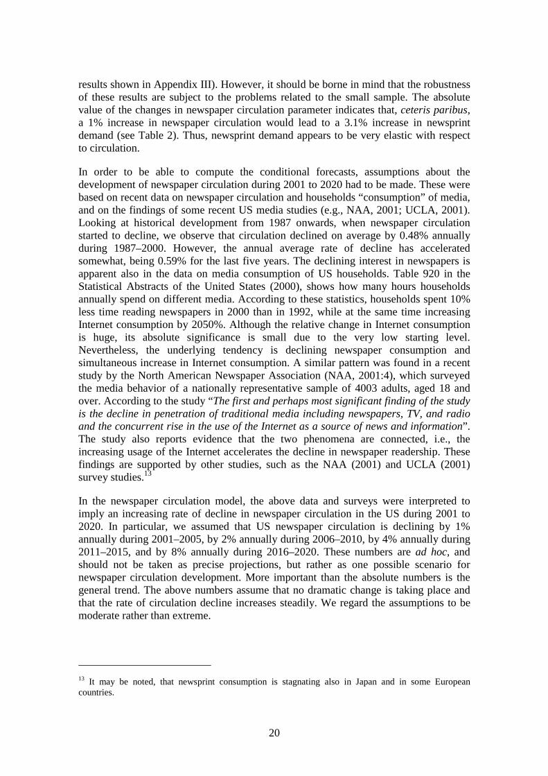
The dynamic forecasts of the newspaper circulation model based on the aboveassumptions are shown in Figure 9. According to the projection, newsprint consumptionis declining rather steadily up to 2010, after which the speed of decline increases. Thispattern clearly reflects the assumptions made about the newspaper circulation decline.The newsprint circulation model forecast that in 2020 the newsprint consumption wouldbe 7.6 million tons, which is equivalent to the level last experienced in the mid-1960s.
7
8
9
10
11
12
13
00 02 04 06 08 10 12 14 16 18 20
Model 9
7.6
mill. tons
Year
Figure 9: Forecasts from newspaper circulation model, 2001–2020.
5.5 Comparing the Forecasts
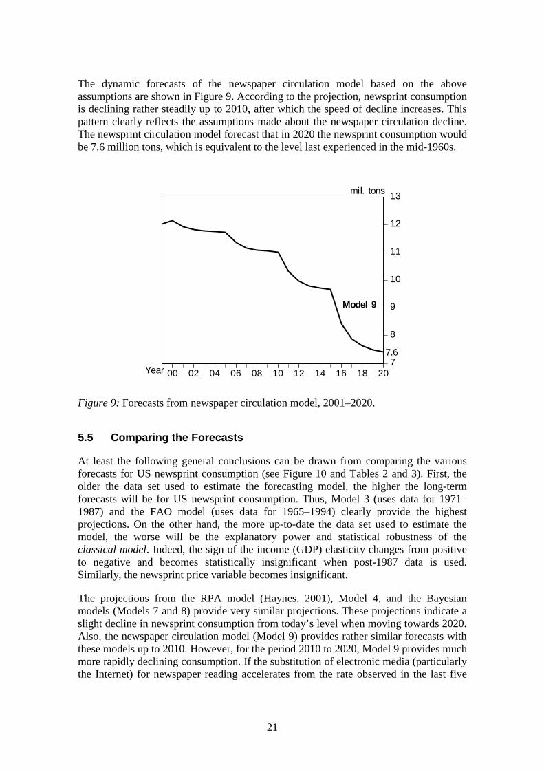
At least the following general conclusions can be drawn from comparing the variousforecasts for US newsprint consumption (see Figure 10 and Tables 2 and 3). First, theolder the data set used to estimate the forecasting model, the higher the long-termforecasts will be for US newsprint consumption. Thus, Model 3 (uses data for 1971–1987) and the FAO model (uses data for 1965–1994) clearly provide the highestprojections. On the other hand, the more up-to-date the data set used to estimate themodel, the worse will be the explanatory power and statistical robustness of theclassical model. Indeed, the sign of the income (GDP) elasticity changes from positiveto negative and becomes statistically insignificant when post-1987 data is used.Similarly, the newsprint price variable becomes insignificant.
The projections from the RPA model (Haynes, 2001), Model 4, and the Bayesianmodels (Models 7 and 8) provide very similar projections. These projections indicate aslight decline in newsprint consumption from today’s level when moving towards 2020.Also, the newspaper circulation model (Model 9) provides rather similar forecasts withthese models up to 2010. However, for the period 2010 to 2020, Model 9 provides muchmore rapidly declining consumption. If the substitution of electronic media (particularlythe Internet) for newspaper reading accelerates from the rate observed in the last five
22
years or so, the projections of Model 9 may very well turn out to be the most accurate ofthe various projections presented in this study.
8
10
12
14
16
75 80 85 90 95 00 05 10 15 20
FAO
Model 4
Model 8
RPA
Model 9
mill. tons
Year
16.4
7.4
Figure 10: Forecasts from various models.
From the practical policy perspective, the differences in the projections are significantand troubling. Depending on whether newsprint consumption will follow the FAOprojection or instead that of Model 9 or even the RPA projection, very differentadjustments would be required in the US newsprint production and its imports (mainlyfrom Canada). The FAO projection would imply more or less the “business-as-usual”pattern for the newsprint industry, while the Model 9 projection would imply major cutsin domestic productions and imports.
6 Summary and Conclusions
In the present study, forecasts for the US newsprint demand for 2001 to 2020 werecomputed using various approaches. The results shed light both on the methodologicalquestions relating to modeling newsprint demand, as well as providing new forecasts fornewsprint consumption.
The results indicated that the classical forest products demand model, still commonlyused in forest economics literature, could not explain or forecast the recent structuralchange in the US newsprint consumption. Both the income (GDP) and newsprint pricevariable turned out to be insignificant determinants of newsprint demand. Moreover, theresults of this study indicate that one should not rule out the possibility of negative
23
income elasticity. However, the negative sign of the income elasticity is usuallyinterpreted in the literature to be inconsistent with the demand theory and reflect anerror in the model, estimation, or data (Simangunsong and Buongiorno, 2001;Buongiorno et al., 2001). So far, this may not have been a particularly large issue, sincein the literature negative income elasticities for forest products demand are rarelyreported. For example, Simangunsong and Buongiorno (2001) summarize the resultsfrom 9 studies published between 1978 and 2000, and the results show that for the 10different forest product categories covered (including newsprint), not a single negativeincome elasticity was obtained.
Recent data and studies on the US media behavior point out that people read lessnewspapers, while simultaneously increasing the consumption of electronic media,especially the Internet (NAA, 2001; UCLA, 2001). It may be that economic wealth (i.e.,GDP) is one of the factors that allow this substitution to take place. The higher the GDP,the more wealth households have to buy relative expensive computers and the servicesrequired, such as Internet accounts and modems. Also, the more households there arewith access to the Internet, the more likely that there is substitution between printednewspapers and consumption of the Internet. Thus, this could imply negative incomeelasticity of demand for newsprint. On the other hand, it may be the case that at someincome level newsprint consumption starts to be independent of income. Our estimationresults suggest that the latter conclusion may be relevant for the US today.
In order to resolve the problems relating to the classical newsprint demand model, weproposed two alternative approaches ― the Bayesian model and the newspapercirculation model. The Bayesian model allowed combining historical data with“forward looking” information concerning the GDP elasticity. This model should,however, be regarded more as an illustrative case of the Bayesian approach in a familiarclassical setting, rather than a genuine alternative to the classical model. This means itpresented a methodology that allows forest sector analysts to incorporate the ‘future’into the conventional classical demand model by using informed prior. In future studies,the Bayesian approach could be extended in a number of ways that would differentiate itmore clearly from the classical framework.
The newspaper circulation model is clearly an alternative to the classical model, sinceneither the GDP nor the newsprint price variable are included in forecasting long-termnewsprint consumption. On the basis of pragmatic reasoning and data analysis, it wasconcluded that the changes in newspaper circulations could be an important indicator offuture newsprint consumption. Consequently, an ad hoc newspaper circulation modelwas formulated and estimated. This very simple model performed rather well. However,a challenge remains in the future to extend the model to also include variables that couldaccount for the changes in the size and grammage of newspapers. The latter factors willalso directly affect the demand for newsprint. For example, the size of the averageprinted version of a newspaper and the grammage of newsprint is likely to decreaseduring 2001 to 2020. The major driving force behind this is the movement ofadvertisements (specially classified) to other media, and changes in editorial and othercontent to online-newspapers. Thus, these factors will most likely enhance the decliningtrend of newsprint demand.

24
The general conclusion from the study is that US newsprint consumption is more likelyto decline than increase in the long-term. Of the various model specifications, thenewsprint circulation model provided the lowest forecasts ― 7.6 million tons for 2020― which is equivalent of the level last experienced in the mid-1960s.
REFERENCESAdams, D. and R. Haynes (1980). The 1980 Softwood Timber Assessment Market
Model: Structure, Projections, and Policy Simulation. Forest Science Monograph,22.
Allen, G. and R. Fields (1999). Econometric Forecasting Principles and Doubts: UnitRoot Testing First, Last, or Never? Presented at the 19th International Symposiumon Forecasting, 27–30 June 1999, Washington, DC, USA.
Baudin, A. and D. Brooks (1995). Projections of Forest Products Demand, Supply andTrade in ETTS V. ECE/TIM/DP/6. United Nations Economic Commission forEurope, Geneva, Switzerland.
Bauwens, L., M. Lubrano and J.-F. Richard (1999). Bayesian Inference in DynamicEconometric Models. Oxford University Press, UK.
Buongiorno, J. (1977). Long-Term Forecasting of Major Forest Products Consumptionin Developed and Developing Economies. Forest Science, Vol. 23, No. 1, pp. 13–25.
Buongiorno, J. (1996). Forest Sector Modeling: A Synthesis of Econometrics,Mathematical Programming, and System Dynamics Methods. InternationalJournal of Forecasting, Vol. 12, pp. 329–343.
Buongiorno, J., C.-S. Liu and J. Turner (2001). Estimating International Wood andFiber Utilization Accounts in the Presence of Measurement Errors. Journal ofForest Economics, 7:2, pp. 101–128.
FAO (1999a). Global Forest Products Consumption, Production, Trade and Prices:Global Forest Products Model Projections to 2010. Working PaperGFPOS/WP/01, Food and Agriculture Organization of the United Nations (FAO),Rome, Italy.
FAO (1999b). The Global Forest Products Model (GFPM): Users Manual and Guide toInstallation. Working Paper GFPOS/WP/02, Food and Agriculture Organizationof the United Nations (FAO), Rome, Italy.
Fernandez, C., E. Ley and M. Steel (2001). Model Uncertainty in Cross-country GrowthRegressions. Journal of Applied Econometrics, Vol. 16, Issue 5, pp. 563–576.
Hamilton, J.D. (1994). Time Series Analysis. Princeton University Press, Princeton,USA.
Haynes, R. (2001). An Analysis of the Timber Situation in the United States:1997-2050. General Technical Report PNW-GTR-xxx. USDA Forest Service,Pacific Northwest Research Station, Portland, Oregon, USA, forthcoming.

25
Hendry, D.F. and J.A. Doornik (1997). Empirical Econometric Modelling using PcGive9.0 for Windows. International Thomson Business Press, London, UK.
Kallio, M., D.P. Dykstra and C. Binkley, eds. (1987). The Global Forest Sector: AnAnalytical Perspective. Wiley, New York, USA.
Lutz, W. and A. Goujon (2001). The World’s Changing Human Capital Stock: Multi-State Population Projection by Educational Attainment. Population andDevelopment Review, 27(2), pp. 323–339, June.
McKillop, W.L.M. (1967). Supply and Demand for Forest Products ― An EconometricStudy. Hilgardia, 38 (1), pp. 1–132.
NAA (2001). Leveraging Newspaper Assets: A Study of Changing American MediaUsage Habits, 2000. Research Report. Downloaded from and available on theInternet: http://www.naa.org. October 2001.
Obersteiner, M. (1998). The Pan Siberian Forest Industry Model (PSFIM): ATheoretical Concept for Forest Industry Analysis. Interim Report IR-98-033.International Institute for Applied Systems Analysis, Laxenburg, Austria.
Obersteiner, M. and S. Nilsson (2000). Press-imistic Futures? ― Science BasedConcepts and Models to Assess the Long-term Competitiveness of Paper Productsin the Information Age. Interim Report IR-00-059. International Institute forApplied Systems Analysis, Laxenburg, Austria.
Pole, A., M. West and J. Harrison (1999). Applied Bayesian Forecasting and TimeSeries Analysis. Chapman and Hall, USA.
Pringle, S. (1954). An Econometric Analysis of the Demand for Newsprint in the UnitedStates. Ph.D. Dissertation, Syracuse University, USA.
Procter, A. (2000). Managing Technology for Value Delivery. Course Manuscript,Department of Wood Science, University of British Columbia, Vancouver,Canada.
Simangunsong, B.C.H. and J. Buongiorno (2001). International Demand Equations forForest Products: A Comparison of Methods. Scandinavian Journal of ForestResearch, 16, pp. 155–172.
Solberg, B. and A. Moiseyev, eds. (1997). Demand and Supply Analyses ofRoundwood and Forest Products Markets in Europe ― Overview of PresentStudies. First Workshop of the Concerted Action Project AIR3-CT942288,Helsinki, Finland, 3–5 November 1995, Helsinki, 1997. EFI Proceedings No. 17,European Forest Institute (EFI), Helsinki, Finland, 418 p.
Statistical Abstracts of the United States (2000). US Census Bureau. Downloaded fromand available on the Internet: http://www.census.gov/statab/www/.
UCLA (2001). Surveying the Digital Future: Year Two. University of California, LosAngeles (UCLA) Internet Report 2001, Center for Communication Policy.Downloaded from and available on the Internet: http://ccp.ucla.edu, 29 November2001.
West, M. and J. Harrison (1997). Bayesian Forecasting and Dynamic Models.Springer-Verlag Series in Statistics, USA.

26
Zhang, Y. and J. Buongiorno (1997). Communication Media and Demand for Printingand Publishing Papers in the United States. Forest Science, Vol. 43, No. 3, pp.362–377.
Zhang, Y., J. Buongiorno and P. Ince (1993). PELPS III: A Microcomputer Price-endogenous Linear Programming System for Economic Modeling. ResearchPaper FPL-RP-526. USDA Forest Service, Forest Product Laboratory, Madison,Wisconsin, USA.
27
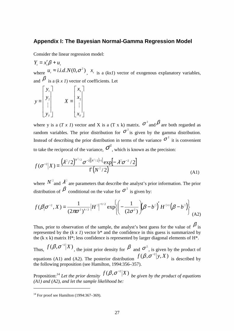
Appendix I: The Bayesian Normal-Gamma Regression Model
Consider the linear regression model:
ttt uxY +′= β
where ),0(... 2σNdiiut ≈ , tx is a (kx1) vector of exogenous explanatory variables,
and β is a (k x 1) vector of coefficients. Let
=
=
TT x
x
x
X
y
y
y
yMM2
1
2
1
where y is a (T x 1) vector and X is a (T x k) matrix.2σ and β are both regarded as
random variables. The prior distribution for2σ is given by the gamma distribution.
Instead of describing the prior distribution in terms of the variance2σ it is convenient
to take the reciprocal of the variance,2−σ , which is known as the precision:
( ) ( )[ ] [ ]( )2/
2/exp2/)(
212/22/
2
∗
−∗−−∗−
Γ−=
∗∗
NXf
NN σλσλσ(A1)
where∗N and
∗λ are parameters that describe the analyst’s prior information. The prior
distribution of β conditional on the value for2σ is given by:
( ) ( )
−′−
−= ∗−∗∗−∗− bHbHXf
kββ
σπσσβ 1
2
2/1
2/2
2
)2(
1exp
)2(
1),(
(A2)
Thus, prior to observation of the sample, the analyst’s best guess for the value of β isrepresented by the (k x 1) vector b* and the confidence in this guess is summarized bythe (k x k) matrix H*; less confidence is represented by larger diagonal elements of H*.
Thus,),( 2 Xf −σβ
, the joint prior density for β and2σ , is given by the product of
equations (A1) and (A2). The posterior distribution),,( 2 Xyf −σβ
is described bythe following proposition (see Hamilton, 1994:356–357).
Proposition:14 Let the prior density),( 2 Xf −σβ
be given by the product of equations(A1) and (A2), and let the sample likelihood be:
14 For proof see Hamilton (1994:367–369).
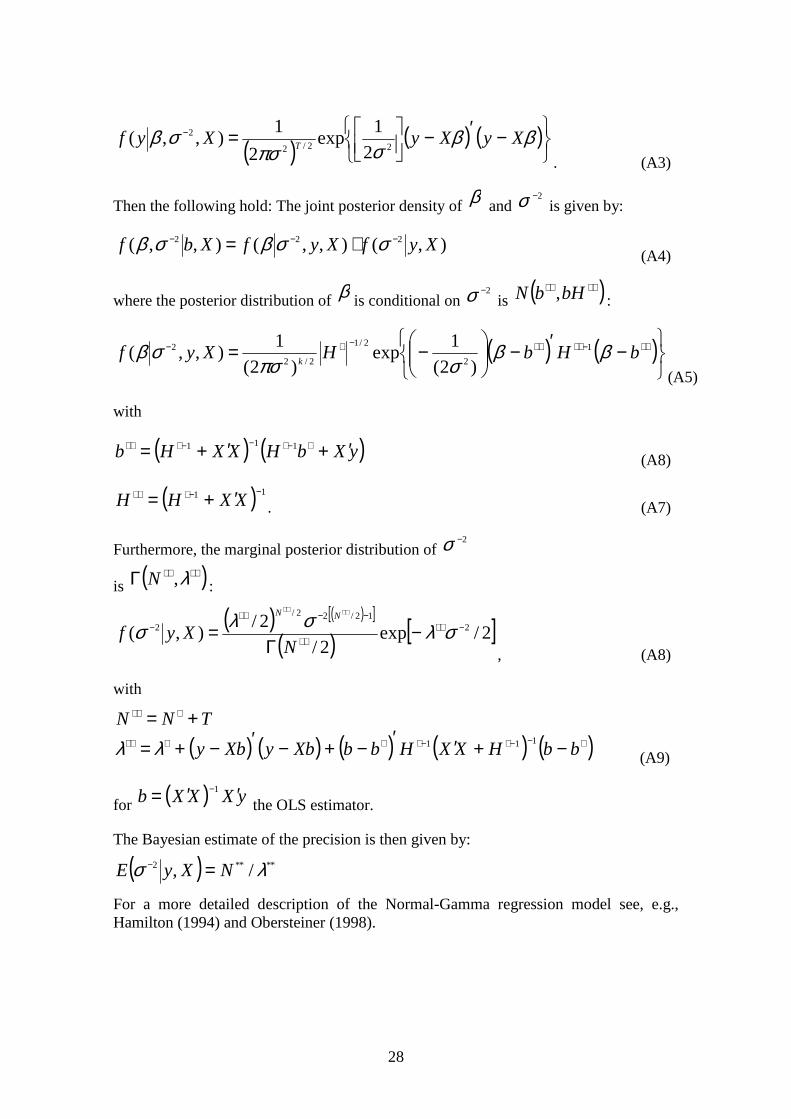
28
( ) ( ) ( )
−′−
=− ββ
σπσσβ XyXyXyf T 22/2
2
2
1exp
2
1),,(
. (A3)
Then the following hold: The joint posterior density of β and2−σ is given by:
),(),,(),,( 222 XyfXyfXbf −−− ⋅= σσβσβ(A4)
where the posterior distribution of β is conditional on2−σ is ( )∗∗∗∗ bHbN , :
( ) ( )
−′−
−= ∗∗−∗∗∗∗−∗− bHbHXyfk
ββσπσ
σβ 1
2
2/1
2/2
2
)2(
1exp
)2(
1),,(
(A5)
with
( ) ( )yXbHXXHb ′+′+= ∗−∗−−∗∗∗ 111
(A8)
( ) 11 −−∗∗∗ ′+= XXHH . (A7)
Furthermore, the marginal posterior distribution of2−σ
is ( )∗∗∗∗Γ λ,N :
( ) ( )[ ]
( ) [ ]2/exp2/
2/),( 2
12/22/
2 −∗∗∗∗
−−∗∗− −
Γ=
∗∗∗∗
σλσλσN
XyfNN
, (A8)
with
TNN += ∗∗∗
( ) ( ) ( ) ( ) ( )∗−−∗−∗∗∗∗∗ −+′′−+−′−+= bbHXXHbbXbyXby111λλ (A9)
for ( ) yXXXb ′′= −1
the OLS estimator.
The Bayesian estimate of the precision is then given by:
( ) ****2 /, λσ NXyE =−
For a more detailed description of the Normal-Gamma regression model see, e.g.,Hamilton (1994) and Obersteiner (1998).
29
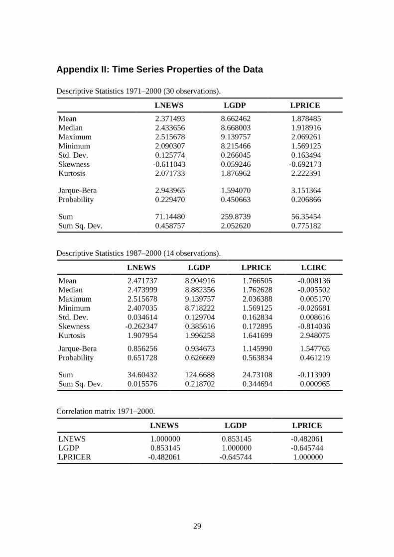
Appendix II: Time Series Properties of the Data
Descriptive Statistics 1971–2000 (30 observations).
LNEWS LGDP LPRICE
Mean 2.371493 8.662462 1.878485Median 2.433656 8.668003 1.918916Maximum 2.515678 9.139757 2.069261Minimum 2.090307 8.215466 1.569125Std. Dev. 0.125774 0.266045 0.163494Skewness -0.611043 0.059246 -0.692173Kurtosis 2.071733 1.876962 2.222391
Jarque-Bera 2.943965 1.594070 3.151364Probability 0.229470 0.450663 0.206866
Sum 71.14480 259.8739 56.35454Sum Sq. Dev. 0.458757 2.052620 0.775182
Descriptive Statistics 1987–2000 (14 observations).
LNEWS LGDP LPRICE LCIRC
Mean 2.471737 8.904916 1.766505 -0.008136Median 2.473999 8.882356 1.762628 -0.005502Maximum 2.515678 9.139757 2.036388 0.005170Minimum 2.407035 8.718222 1.569125 -0.026681Std. Dev. 0.034614 0.129704 0.162834 0.008616Skewness -0.262347 0.385616 0.172895 -0.814036Kurtosis 1.907954 1.996258 1.641699 2.948075
Jarque-Bera 0.856256 0.934673 1.145990 1.547765Probability 0.651728 0.626669 0.563834 0.461219
Sum 34.60432 124.6688 24.73108 -0.113909Sum Sq. Dev. 0.015576 0.218702 0.344694 0.000965
Correlation matrix 1971–2000.
LNEWS LGDP LPRICE
LNEWS 1.000000 0.853145 -0.482061LGDP 0.853145 1.000000 -0.645744LPRICER -0.482061 -0.645744 1.000000
30
Correlation matrix 1971–1987.
LNEWS LGDP LPRICE
LNEWS 1.000000 0.914902 -0.086354LGDP 0.914902 1.000000 0.273656LPRICER -0.086354 0.273656 1.000000
Correlation matrix 1987–2000.
LNEWS LGDP LPRICE LCIRC
LNEWS 1.000000 -0.245365 0.295374 0.836755LGDP -0.245365 1.000000 -0.555644 -0.115412LPRICER 0.295374 -0.555644 1.000000 0.071325LCIRCCH 0.836755 -0.115412 0.071325 1.000000
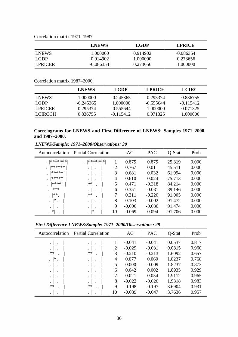
Correlograms for LNEWS and First Difference of LNEWS: Samples 1971–2000and 1987–2000.
LNEWS/Sample: 1971–2000/Observations: 30
Autocorrelation Partial Correlation AC PAC Q-Stat Prob
. |*******| . |*******| 1 0.875 0.875 25.319 0.000. |****** | . | . | 2 0.767 0.011 45.511 0.000. |***** | . | . | 3 0.681 0.032 61.994 0.000. |***** | . | . | 4 0.610 0.024 75.713 0.000. |**** | .**| . | 5 0.471 -0.318 84.214 0.000. |*** | . | . | 6 0.351 -0.031 89.146 0.000. |**. | .**| . | 7 0.211 -0.220 91.005 0.000. |* . | . | . | 8 0.103 -0.002 91.472 0.000. | . | . | . | 9 -0.006 -0.036 91.474 0.000. *| . | . |* . | 10 -0.069 0.094 91.706 0.000
First Difference LNEWS/Sample: 1971–2000/Observations: 29
Autocorrelation Partial Correlation AC PAC Q-Stat Prob
. | . | . | . | 1 -0.041 -0.041 0.0537 0.817
. | . | . | . | 2 -0.029 -0.031 0.0815 0.960.**| . | .**| . | 3 -0.210 -0.213 1.6092 0.657. |* . | . | . | 4 0.077 0.060 1.8237 0.768. | . | . | . | 5 0.000 -0.009 1.8237 0.873. | . | . | . | 6 0.042 0.002 1.8935 0.929. | . | . | . | 7 0.021 0.054 1.9112 0.965. | . | . | . | 8 -0.022 -0.026 1.9318 0.983.**| . | .**| . | 9 -0.198 -0.197 3.6904 0.931. | . | . | . | 10 -0.039 -0.047 3.7636 0.957
31
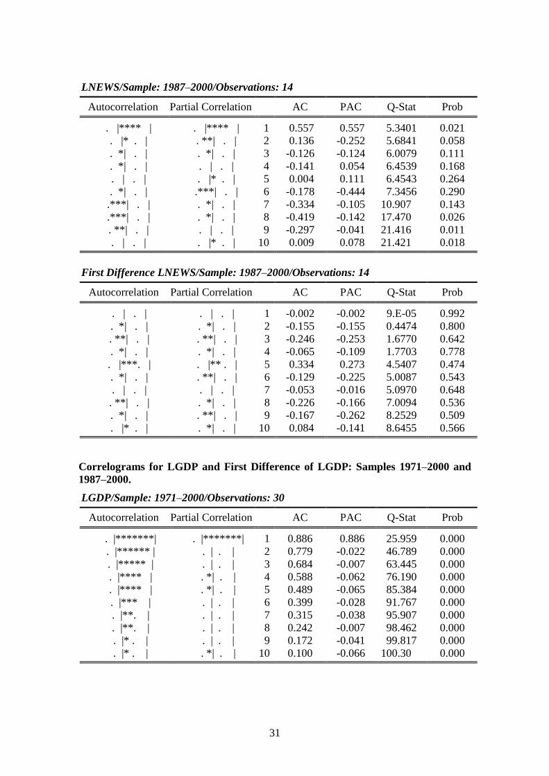
LNEWS/Sample: 1987–2000/Observations: 14
Autocorrelation Partial Correlation AC PAC Q-Stat Prob
. |**** | . |**** | 1 0.557 0.557 5.3401 0.021. |* . | . **| . | 2 0.136 -0.252 5.6841 0.058. *| . | . *| . | 3 -0.126 -0.124 6.0079 0.111. *| . | . | . | 4 -0.141 0.054 6.4539 0.168. | . | . |* . | 5 0.004 0.111 6.4543 0.264. *| . | .***| . | 6 -0.178 -0.444 7.3456 0.290.***| . | . *| . | 7 -0.334 -0.105 10.907 0.143.***| . | . *| . | 8 -0.419 -0.142 17.470 0.026. **| . | . | . | 9 -0.297 -0.041 21.416 0.011. | . | . |* . | 10 0.009 0.078 21.421 0.018
First Difference LNEWS/Sample: 1987–2000/Observations: 14
Autocorrelation Partial Correlation AC PAC Q-Stat Prob
. | . | . | . | 1 -0.002 -0.002 9.E-05 0.992. *| . | . *| . | 2 -0.155 -0.155 0.4474 0.800. **| . | . **| . | 3 -0.246 -0.253 1.6770 0.642. *| . | . *| . | 4 -0.065 -0.109 1.7703 0.778. |***. | . |** . | 5 0.334 0.273 4.5407 0.474. *| . | . **| . | 6 -0.129 -0.225 5.0087 0.543. | . | . | . | 7 -0.053 -0.016 5.0970 0.648. **| . | . *| . | 8 -0.226 -0.166 7.0094 0.536. *| . | . **| . | 9 -0.167 -0.262 8.2529 0.509. |* . | . *| . | 10 0.084 -0.141 8.6455 0.566
Correlograms for LGDP and First Difference of LGDP: Samples 1971–2000 and1987–2000.
LGDP/Sample: 1971–2000/Observations: 30
Autocorrelation Partial Correlation AC PAC Q-Stat Prob
. |*******| . |*******| 1 0.886 0.886 25.959 0.000. |****** | . | . | 2 0.779 -0.022 46.789 0.000. |***** | . | . | 3 0.684 -0.007 63.445 0.000. |**** | . *| . | 4 0.588 -0.062 76.190 0.000. |**** | . *| . | 5 0.489 -0.065 85.384 0.000. |*** | . | . | 6 0.399 -0.028 91.767 0.000. |**. | . | . | 7 0.315 -0.038 95.907 0.000. |**. | . | . | 8 0.242 -0.007 98.462 0.000. |* . | . | . | 9 0.172 -0.041 99.817 0.000. |* . | . *| . | 10 0.100 -0.066 100.30 0.000
32
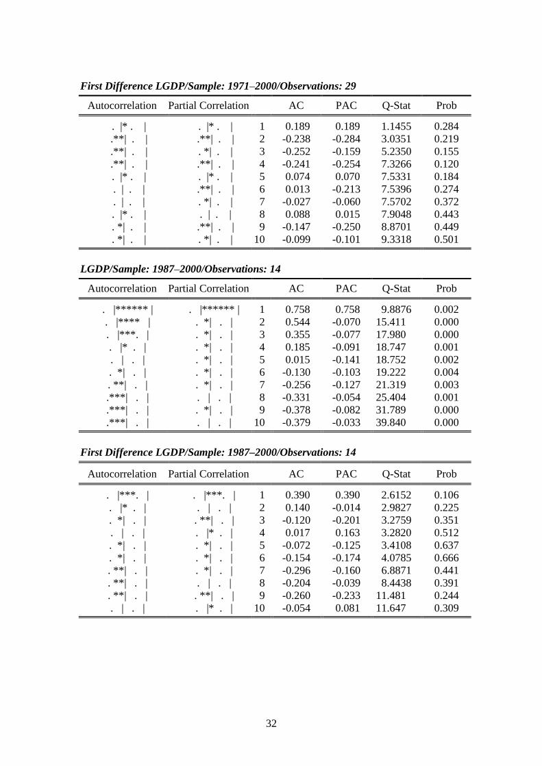
First Difference LGDP/Sample: 1971–2000/Observations: 29
Autocorrelation Partial Correlation AC PAC Q-Stat Prob
. |* . | . |* . | 1 0.189 0.189 1.1455 0.284.**| . | .**| . | 2 -0.238 -0.284 3.0351 0.219.**| . | . *| . | 3 -0.252 -0.159 5.2350 0.155.**| . | .**| . | 4 -0.241 -0.254 7.3266 0.120. |* . | . |* . | 5 0.074 0.070 7.5331 0.184. | . | .**| . | 6 0.013 -0.213 7.5396 0.274. | . | . *| . | 7 -0.027 -0.060 7.5702 0.372. |* . | . | . | 8 0.088 0.015 7.9048 0.443. *| . | .**| . | 9 -0.147 -0.250 8.8701 0.449. *| . | . *| . | 10 -0.099 -0.101 9.3318 0.501
LGDP/Sample: 1987–2000/Observations: 14
Autocorrelation Partial Correlation AC PAC Q-Stat Prob
. |****** | . |****** | 1 0.758 0.758 9.8876 0.002. |**** | . *| . | 2 0.544 -0.070 15.411 0.000. |***. | . *| . | 3 0.355 -0.077 17.980 0.000. |* . | . *| . | 4 0.185 -0.091 18.747 0.001. | . | . *| . | 5 0.015 -0.141 18.752 0.002. *| . | . *| . | 6 -0.130 -0.103 19.222 0.004. **| . | . *| . | 7 -0.256 -0.127 21.319 0.003.***| . | . | . | 8 -0.331 -0.054 25.404 0.001.***| . | . *| . | 9 -0.378 -0.082 31.789 0.000.***| . | . | . | 10 -0.379 -0.033 39.840 0.000
First Difference LGDP/Sample: 1987–2000/Observations: 14
Autocorrelation Partial Correlation AC PAC Q-Stat Prob
. |***. | . |***. | 1 0.390 0.390 2.6152 0.106. |* . | . | . | 2 0.140 -0.014 2.9827 0.225. *| . | . **| . | 3 -0.120 -0.201 3.2759 0.351. | . | . |* . | 4 0.017 0.163 3.2820 0.512. *| . | . *| . | 5 -0.072 -0.125 3.4108 0.637. *| . | . *| . | 6 -0.154 -0.174 4.0785 0.666. **| . | . *| . | 7 -0.296 -0.160 6.8871 0.441. **| . | . | . | 8 -0.204 -0.039 8.4438 0.391. **| . | . **| . | 9 -0.260 -0.233 11.481 0.244. | . | . |* . | 10 -0.054 0.081 11.647 0.309
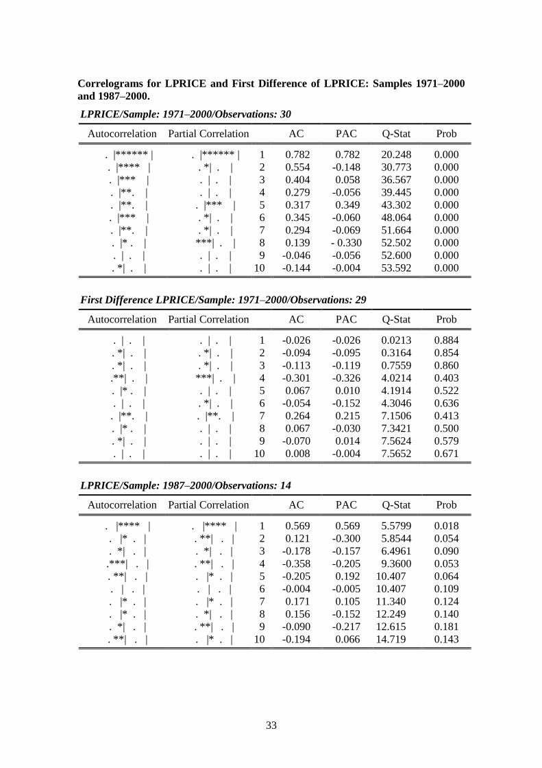
33
Correlograms for LPRICE and First Difference of LPRICE: Samples 1971–2000and 1987–2000.
LPRICE/Sample: 1971–2000/Observations: 30
Autocorrelation Partial Correlation AC PAC Q-Stat Prob
. |****** | . |****** | 1 0.782 0.782 20.248 0.000. |**** | . *| . | 2 0.554 -0.148 30.773 0.000. |*** | . | . | 3 0.404 0.058 36.567 0.000. |**. | . | . | 4 0.279 -0.056 39.445 0.000. |**. | . |*** | 5 0.317 0.349 43.302 0.000. |*** | . *| . | 6 0.345 -0.060 48.064 0.000. |**. | . *| . | 7 0.294 -0.069 51.664 0.000. |* . | ***| . | 8 0.139 - 0.330 52.502 0.000. | . | . | . | 9 -0.046 -0.056 52.600 0.000. *| . | . | . | 10 -0.144 -0.004 53.592 0.000
First Difference LPRICE/Sample: 1971–2000/Observations: 29
Autocorrelation Partial Correlation AC PAC Q-Stat Prob
. | . | . | . | 1 -0.026 -0.026 0.0213 0.884. *| . | . *| . | 2 -0.094 -0.095 0.3164 0.854. *| . | . *| . | 3 -0.113 -0.119 0.7559 0.860.**| . | ***| . | 4 -0.301 -0.326 4.0214 0.403. |* . | . | . | 5 0.067 0.010 4.1914 0.522. | . | . *| . | 6 -0.054 -0.152 4.3046 0.636. |**. | . |**. | 7 0.264 0.215 7.1506 0.413. |* . | . | . | 8 0.067 -0.030 7.3421 0.500. *| . | . | . | 9 -0.070 0.014 7.5624 0.579. | . | . | . | 10 0.008 -0.004 7.5652 0.671
LPRICE/Sample: 1987–2000/Observations: 14
Autocorrelation Partial Correlation AC PAC Q-Stat Prob
. |**** | . |**** | 1 0.569 0.569 5.5799 0.018. |* . | . **| . | 2 0.121 -0.300 5.8544 0.054. *| . | . *| . | 3 -0.178 -0.157 6.4961 0.090.***| . | . **| . | 4 -0.358 -0.205 9.3600 0.053. **| . | . |* . | 5 -0.205 0.192 10.407 0.064. | . | . | . | 6 -0.004 -0.005 10.407 0.109. |* . | . |* . | 7 0.171 0.105 11.340 0.124. |* . | . *| . | 8 0.156 -0.152 12.249 0.140. *| . | . **| . | 9 -0.090 -0.217 12.615 0.181. **| . | . |* . | 10 -0.194 0.066 14.719 0.143
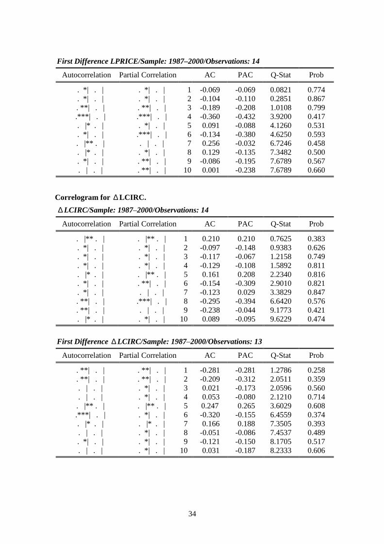
34
Correlogram for ∆ LCIRC.
∆ LCIRC/Sample: 1987–2000/Observations: 14
Autocorrelation Partial Correlation AC PAC Q-Stat Prob
. |** . | . |** . | 1 0.210 0.210 0.7625 0.383. *| . | . *| . | 2 -0.097 -0.148 0.9383 0.626. *| . | . *| . | 3 -0.117 -0.067 1.2158 0.749. *| . | . *| . | 4 -0.129 -0.108 1.5892 0.811. |* . | . |** . | 5 0.161 0.208 2.2340 0.816. *| . | . **| . | 6 -0.154 -0.309 2.9010 0.821. *| . | . | . | 7 -0.123 0.029 3.3829 0.847. **| . | .***| . | 8 -0.295 -0.394 6.6420 0.576. **| . | . | . | 9 -0.238 -0.044 9.1773 0.421. |* . | . *| . | 10 0.089 -0.095 9.6229 0.474
First Difference ∆ LCIRC/Sample: 1987–2000/Observations: 13
Autocorrelation Partial Correlation AC PAC Q-Stat Prob
. **| . | . **| . | 1 -0.281 -0.281 1.2786 0.258
. **| . | . **| . | 2 -0.209 -0.312 2.0511 0.359. | . | . *| . | 3 0.021 -0.173 2.0596 0.560. | . | . *| . | 4 0.053 -0.080 2.1210 0.714. |** . | . |** . | 5 0.247 0.265 3.6029 0.608.***| . | . *| . | 6 -0.320 -0.155 6.4559 0.374. |* . | . |* . | 7 0.166 0.188 7.3505 0.393. | . | . *| . | 8 -0.051 -0.086 7.4537 0.489. *| . | . *| . | 9 -0.121 -0.150 8.1705 0.517. | . | . *| . | 10 0.031 -0.187 8.2333 0.606
First Difference LPRICE/Sample: 1987–2000/Observations: 14
Autocorrelation Partial Correlation AC PAC Q-Stat Prob
. *| . | . *| . | 1 -0.069 -0.069 0.0821 0.774
. *| . | . *| . | 2 -0.104 -0.110 0.2851 0.867. **| . | . **| . | 3 -0.189 -0.208 1.0108 0.799.***| . | .***| . | 4 -0.360 -0.432 3.9200 0.417. |* . | . *| . | 5 0.091 -0.088 4.1260 0.531. *| . | .***| . | 6 -0.134 -0.380 4.6250 0.593. |** . | . | . | 7 0.256 -0.032 6.7246 0.458. |* . | . *| . | 8 0.129 -0.135 7.3482 0.500. *| . | . **| . | 9 -0.086 -0.195 7.6789 0.567. | . | . **| . | 10 0.001 -0.238 7.6789 0.660
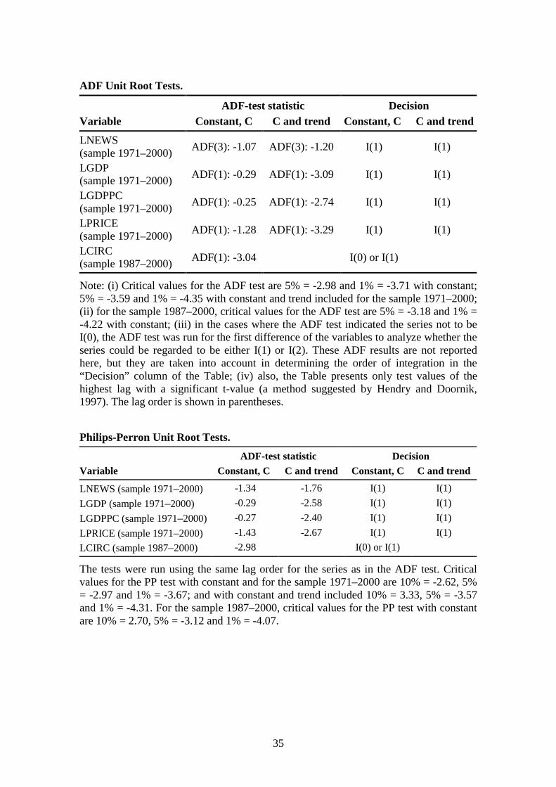
35
ADF Unit Root Tests.
ADF-test statistic DecisionVariable Constant, C C and trend Constant, C C and trend
LNEWS(sample 1971–2000)
ADF(3): -1.07 ADF(3): -1.20 I(1) I(1)
LGDP(sample 1971–2000)
ADF(1): -0.29 ADF(1): -3.09 I(1) I(1)
LGDPPC(sample 1971–2000)
ADF(1): -0.25 ADF(1): -2.74 I(1) I(1)
LPRICE(sample 1971–2000)
ADF(1): -1.28 ADF(1): -3.29 I(1) I(1)
LCIRC(sample 1987–2000)
ADF(1): -3.04 I(0) or I(1)
Note: (i) Critical values for the ADF test are 5% = -2.98 and 1% = -3.71 with constant;5% = -3.59 and 1% = -4.35 with constant and trend included for the sample 1971–2000;(ii) for the sample 1987–2000, critical values for the ADF test are 5% = -3.18 and 1% =-4.22 with constant; (iii) in the cases where the ADF test indicated the series not to beI(0), the ADF test was run for the first difference of the variables to analyze whether theseries could be regarded to be either I(1) or I(2). These ADF results are not reportedhere, but they are taken into account in determining the order of integration in the“Decision” column of the Table; (iv) also, the Table presents only test values of thehighest lag with a significant t-value (a method suggested by Hendry and Doornik,1997). The lag order is shown in parentheses.
Philips-Perron Unit Root Tests.
ADF-test statistic DecisionVariable Constant, C C and trend Constant, C C and trend
LNEWS (sample 1971–2000) -1.34 -1.76 I(1) I(1)
LGDP (sample 1971–2000) -0.29 -2.58 I(1) I(1)
LGDPPC (sample 1971–2000) -0.27 -2.40 I(1) I(1)
LPRICE (sample 1971–2000) -1.43 -2.67 I(1) I(1)
LCIRC (sample 1987–2000) -2.98 I(0) or I(1)
The tests were run using the same lag order for the series as in the ADF test. Criticalvalues for the PP test with constant and for the sample 1971–2000 are 10% = -2.62, 5%= -2.97 and 1% = -3.67; and with constant and trend included 10% = 3.33, 5% = -3.57and 1% = -4.31. For the sample 1987–2000, critical values for the PP test with constantare 10% = 2.70, 5% = -3.12 and 1% = -4.07.
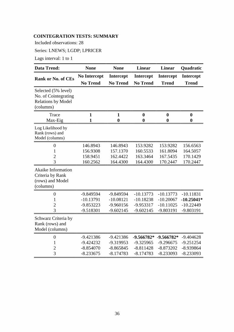
36
COINTEGRATION TESTS: SUMMARYIncluded observations: 28
Series: LNEWS; LGDP; LPRICER
Lags interval: 1 to 1
Data Trend: None None Linear Linear Quadratic
No Intercept Intercept Intercept Intercept InterceptRank or No. of CEs
No Trend No Trend No Trend Trend Trend
Selected (5% level)No. of CointegratingRelations by Model(columns)
Trace 1 1 0 0 0Max-Eig 1 0 0 0 0
Log Likelihood byRank (rows) andModel (columns)
0 146.8943 146.8943 153.9282 153.9282 156.65631 156.9308 157.1370 160.5533 161.8094 164.50572 158.9451 162.4422 163.3464 167.5435 170.14293 160.2562 164.4300 164.4300 170.2447 170.2447
Akaike InformationCriteria by Rank(rows) and Model(columns)
0 -9.849594 -9.849594 -10.13773 -10.13773 -10.118311 -10.13791 -10.08121 -10.18238 -10.20067 -10.25041*2 -9.853223 -9.960156 -9.953317 -10.11025 -10.224493 -9.518301 -9.602145 -9.602145 -9.803191 -9.803191
Schwarz Criteria byRank (rows) andModel (columns)
0 -9.421386 -9.421386 -9.566782* -9.566782* -9.4046281 -9.424232 -9.319953 -9.325965 -9.296675 -9.2512542 -8.854070 -8.865845 -8.811428 -8.873202 -8.9398643 -8.233675 -8.174783 -8.174783 -8.233093 -8.233093
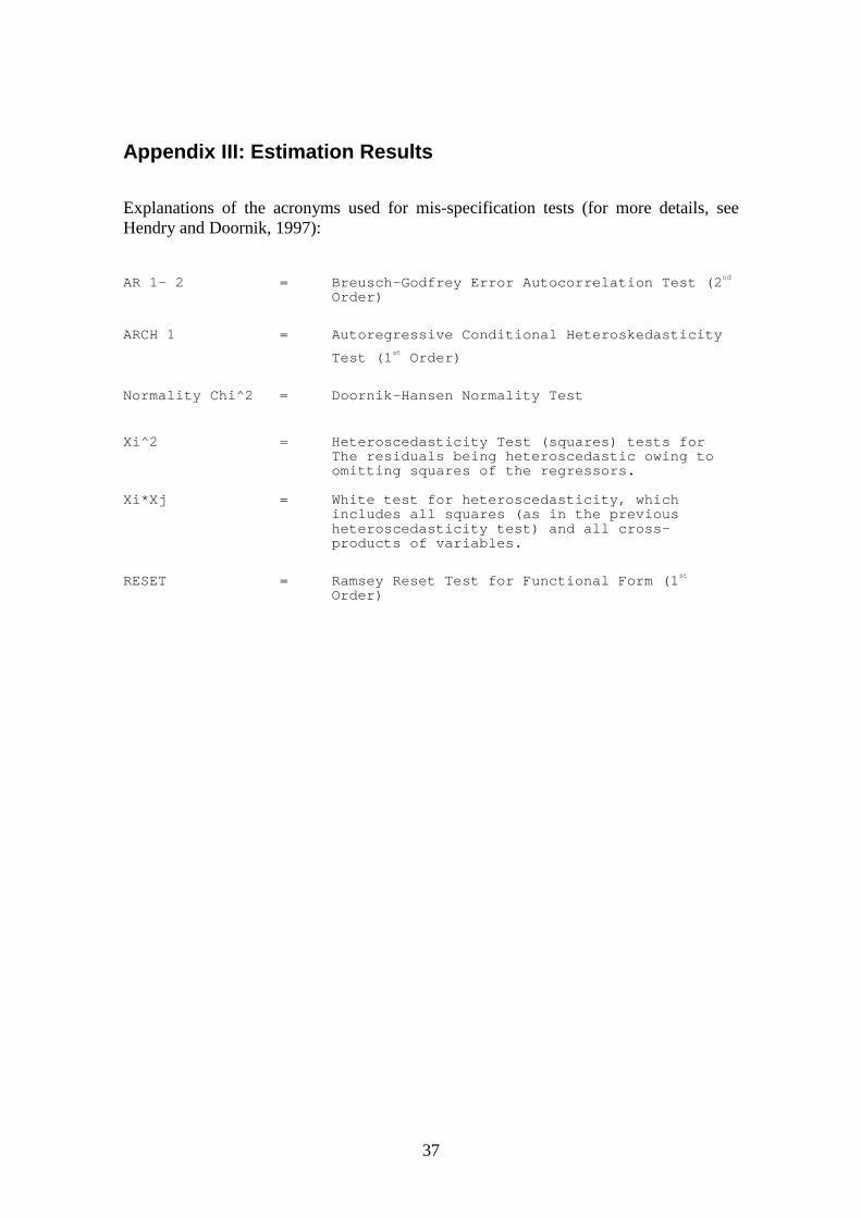
37
Appendix III: Estimation Results
Explanations of the acronyms used for mis-specification tests (for more details, seeHendry and Doornik, 1997):
AR 1- 2 = Breusch-Godfrey Error Autocorrelation Test (2nd
Order)
ARCH 1 = Autoregressive Conditional Heteroskedasticity
Test (1st Order)
Normality Chi^2 = Doornik-Hansen Normality Test
Xi^2 = Heteroscedasticity Test (squares) tests forThe residuals being heteroscedastic owing toomitting squares of the regressors.
Xi*Xj = White test for heteroscedasticity, whichincludes all squares (as in the previousheteroscedasticity test) and all cross-products of variables.
RESET = Ramsey Reset Test for Functional Form (1st
Order)
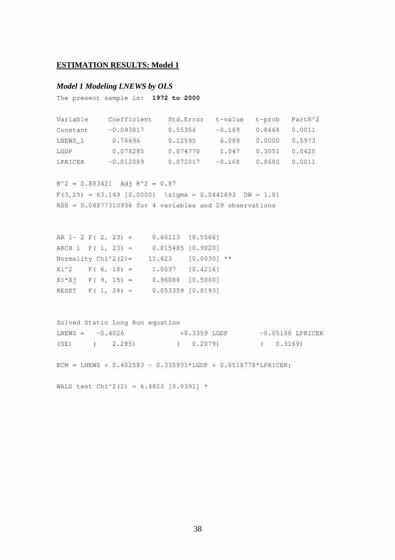
38
ESTIMATION RESULTS: Model 1
Model 1 Modeling LNEWS by OLSThe present sample is: 1972 to 2000
Variable Coefficient Std.Error t-value t-prob PartR^2
Constant -0.093817 0.55356 -0.169 0.8668 0.0011
LNEWS_1 0.76696 0.12595 6.089 0.0000 0.5973
LGDP 0.078285 0.074770 1.047 0.3051 0.0420
LPRICER -0.012089 0.072017 -0.168 0.8680 0.0011
R^2 = 0.883421 Adj R^2 = 0.87
F(3,25) = 63.149 [0.0000] \sigma = 0.0441693 DW = 1.81
RSS = 0.04877310936 for 4 variables and 29 observations
AR 1- 2 F( 2, 23) = 0.60113 [0.5566]
ARCH 1 F( 1, 23) = 0.015485 [0.9020]
Normality Chi^2(2)= 11.623 [0.0030] **
Xi^2 F( 6, 18) = 1.0597 [0.4216]
Xi*Xj F( 9, 15) = 0.96088 [0.5060]
RESET F( 1, 24) = 0.053359 [0.8193]
Solved Static Long Run equation
LNEWS = -0.4026 +0.3359 LGDP -0.05188 LPRICER
(SE) ( 2.285) ( 0.2079) ( 0.3169)
ECM = LNEWS + 0.402583 - 0.335931*LGDP + 0.0518778*LPRICER;
WALD test Chi^2(2) = 6.4823 [0.0391] *
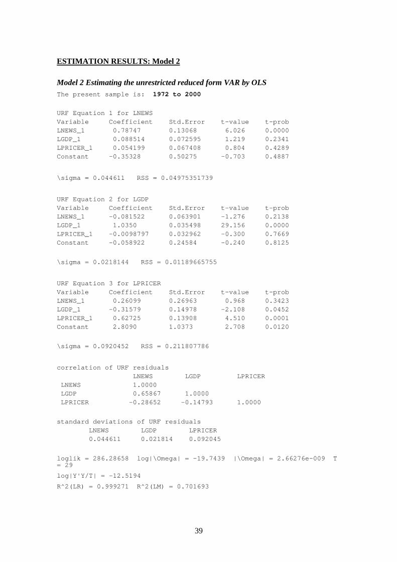
39
ESTIMATION RESULTS: Model 2
Model 2 Estimating the unrestricted reduced form VAR by OLSThe present sample is: 1972 to 2000
URF Equation 1 for LNEWSVariable Coefficient Std.Error t-value t-probLNEWS_1 0.78747 0.13068 6.026 0.0000LGDP_1 0.088514 0.072595 1.219 0.2341LPRICER_1 0.054199 0.067408 0.804 0.4289Constant -0.35328 0.50275 -0.703 0.4887
\sigma = 0.044611 RSS = 0.04975351739
URF Equation 2 for LGDPVariable Coefficient Std.Error t-value t-probLNEWS_1 -0.081522 0.063901 -1.276 0.2138LGDP_1 1.0350 0.035498 29.156 0.0000LPRICER_1 -0.0098797 0.032962 -0.300 0.7669Constant -0.058922 0.24584 -0.240 0.8125
\sigma = 0.0218144 RSS = 0.01189665755
URF Equation 3 for LPRICERVariable Coefficient Std.Error t-value t-probLNEWS_1 0.26099 0.26963 0.968 0.3423LGDP_1 -0.31579 0.14978 -2.108 0.0452LPRICER_1 0.62725 0.13908 4.510 0.0001Constant 2.8090 1.0373 2.708 0.0120
\sigma = 0.0920452 RSS = 0.211807786
correlation of URF residualsLNEWS LGDP LPRICER
LNEWS 1.0000LGDP 0.65867 1.0000LPRICER -0.28652 -0.14793 1.0000
standard deviations of URF residualsLNEWS LGDP LPRICER0.044611 0.021814 0.092045
loglik = 286.28658 log|\Omega| = -19.7439 |\Omega| = 2.66276e-009 T= 29
log|Y'Y/T| = -12.5194
R^2(LR) = 0.999271 R^2(LM) = 0.701693
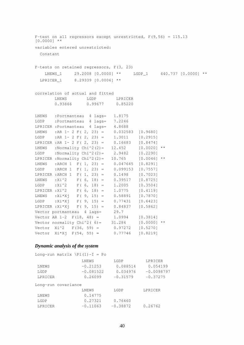
40
F-test on all regressors except unrestricted, F(9,56) = 115.13[0.0000] **
variables entered unrestricted:
Constant
F-tests on retained regressors, F(3, 23)
LNEWS_1 29.2008 [0.0000] ** LGDP_1 440.737 [0.0000] **
LPRICER_1 8.29339 [0.0006] **
correlation of actual and fittedLNEWS LGDP LPRICER0.93866 0.99677 0.85220
LNEWS :Portmanteau 4 lags= 1.8175LGDP :Portmanteau 4 lags= 7.2246LPRICER :Portmanteau 4 lags= 4.8688LNEWS :AR 1- 2 F( 2, 23) = 0.032583 [0.9680]LGDP :AR 1- 2 F( 2, 23) = 1.3011 [0.2915]LPRICER :AR 1- 2 F( 2, 23) = 0.16683 [0.8474]LNEWS :Normality Chi^2(2)= 12.452 [0.0020] **LGDP :Normality Chi^2(2)= 2.9482 [0.2290]LPRICER :Normality Chi^2(2)= 10.765 [0.0046] **LNEWS :ARCH 1 F( 1, 23) = 0.047645 [0.8291]LGDP :ARCH 1 F( 1, 23) = 0.099153 [0.7557]LPRICER :ARCH 1 F( 1, 23) = 0.1498 [0.7023]LNEWS :Xi^2 F( 6, 18) = 0.39517 [0.8725]LGDP :Xi^2 F( 6, 18) = 1.2005 [0.3504]LPRICER :Xi^2 F( 6, 18) = 1.0775 [0.4119]LNEWS :Xi*Xj F( 9, 15) = 0.58891 [0.7870]LGDP :Xi*Xj F( 9, 15) = 0.77431 [0.6423]LPRICER :Xi*Xj F( 9, 15) = 0.84837 [0.5862]Vector portmanteau 4 lags= 29.7Vector AR 1-2 F(18, 48) = 1.0994 [0.3814]Vector normality Chi^2( 6)= 31.284 [0.0000] **Vector Xi^2 F(36, 59) = 0.97272 [0.5270]Vector Xi*Xj F(54, 55) = 0.77746 [0.8219]
Dynamic analysis of the system
Long-run matrix \Pi(1)-I = Po
LNEWS LGDP LPRICERLNEWS -0.21253 0.088514 0.054199LGDP -0.081522 0.034976 -0.0098797LPRICER 0.26099 -0.31579 -0.37275
Long-run covarianceLNEWS LGDP LPRICER
LNEWS 0.14775LGDP 0.27321 0.76460LPRICER -0.11063 -0.38872 0.26762
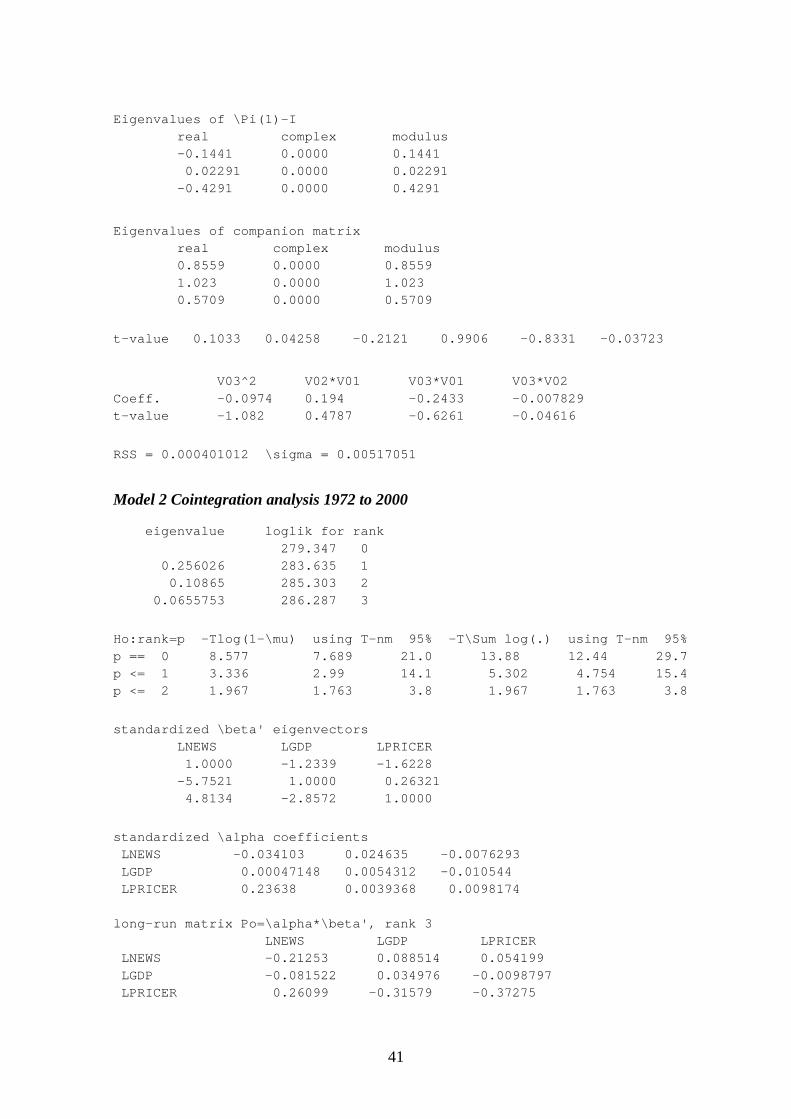
41
Eigenvalues of \Pi(1)-Ireal complex modulus-0.1441 0.0000 0.14410.02291 0.0000 0.02291
-0.4291 0.0000 0.4291
Eigenvalues of companion matrixreal complex modulus0.8559 0.0000 0.85591.023 0.0000 1.0230.5709 0.0000 0.5709
t-value 0.1033 0.04258 -0.2121 0.9906 -0.8331 -0.03723
V03^2 V02*V01 V03*V01 V03*V02Coeff. -0.0974 0.194 -0.2433 -0.007829t-value -1.082 0.4787 -0.6261 -0.04616
RSS = 0.000401012 \sigma = 0.00517051
Model 2 Cointegration analysis 1972 to 2000
eigenvalue loglik for rank279.347 0
0.256026 283.635 10.10865 285.303 2
0.0655753 286.287 3
Ho:rank=p -Tlog(1-\mu) using T-nm 95% -T\Sum log(.) using T-nm 95%p == 0 8.577 7.689 21.0 13.88 12.44 29.7p <= 1 3.336 2.99 14.1 5.302 4.754 15.4p <= 2 1.967 1.763 3.8 1.967 1.763 3.8
standardized \beta' eigenvectorsLNEWS LGDP LPRICER1.0000 -1.2339 -1.6228
-5.7521 1.0000 0.263214.8134 -2.8572 1.0000
standardized \alpha coefficientsLNEWS -0.034103 0.024635 -0.0076293LGDP 0.00047148 0.0054312 -0.010544LPRICER 0.23638 0.0039368 0.0098174
long-run matrix Po=\alpha*\beta', rank 3LNEWS LGDP LPRICER
LNEWS -0.21253 0.088514 0.054199LGDP -0.081522 0.034976 -0.0098797LPRICER 0.26099 -0.31579 -0.37275
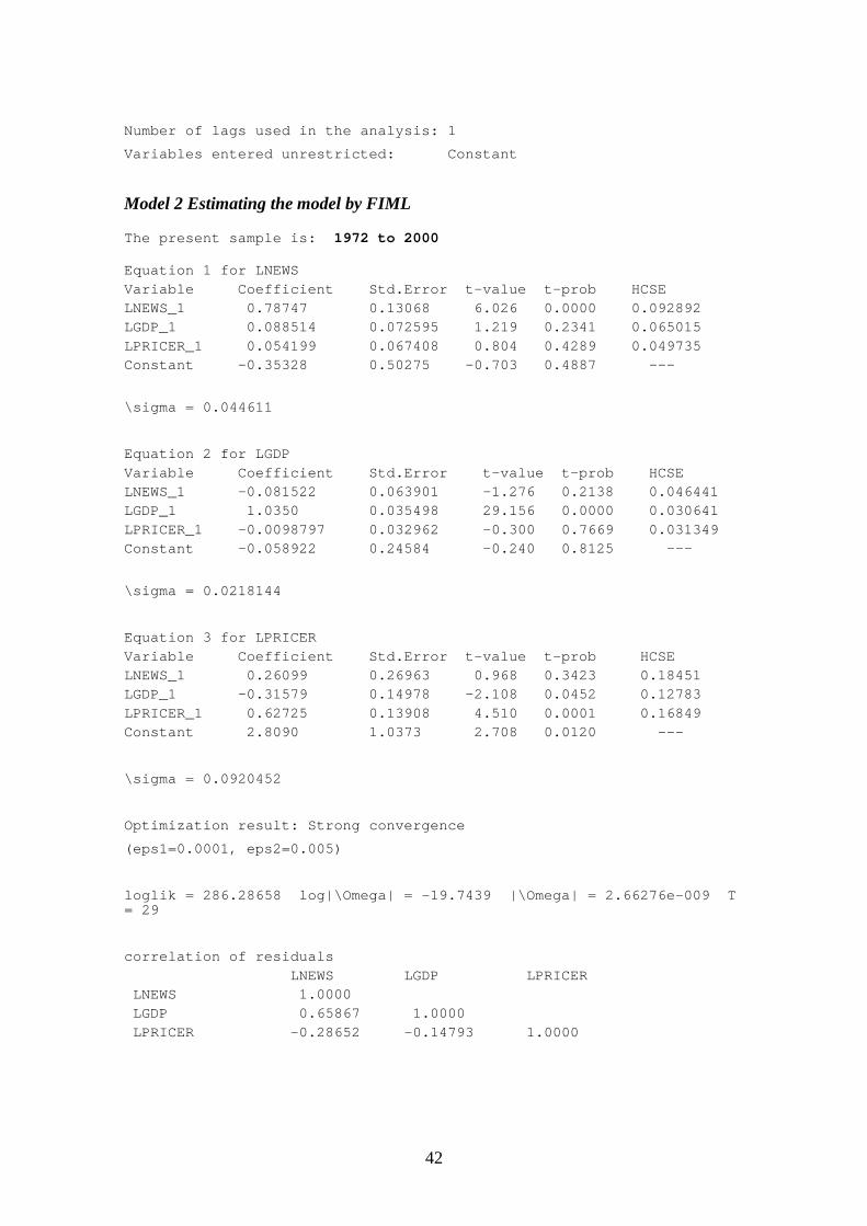
42
Number of lags used in the analysis: 1
Variables entered unrestricted: Constant
Model 2 Estimating the model by FIML
The present sample is: 1972 to 2000
Equation 1 for LNEWSVariable Coefficient Std.Error t-value t-prob HCSELNEWS_1 0.78747 0.13068 6.026 0.0000 0.092892LGDP_1 0.088514 0.072595 1.219 0.2341 0.065015LPRICER_1 0.054199 0.067408 0.804 0.4289 0.049735Constant -0.35328 0.50275 -0.703 0.4887 ---
\sigma = 0.044611
Equation 2 for LGDPVariable Coefficient Std.Error t-value t-prob HCSELNEWS_1 -0.081522 0.063901 -1.276 0.2138 0.046441LGDP_1 1.0350 0.035498 29.156 0.0000 0.030641LPRICER_1 -0.0098797 0.032962 -0.300 0.7669 0.031349Constant -0.058922 0.24584 -0.240 0.8125 ---
\sigma = 0.0218144
Equation 3 for LPRICERVariable Coefficient Std.Error t-value t-prob HCSELNEWS_1 0.26099 0.26963 0.968 0.3423 0.18451LGDP_1 -0.31579 0.14978 -2.108 0.0452 0.12783LPRICER_1 0.62725 0.13908 4.510 0.0001 0.16849Constant 2.8090 1.0373 2.708 0.0120 ---
\sigma = 0.0920452
Optimization result: Strong convergence
(eps1=0.0001, eps2=0.005)
loglik = 286.28658 log|\Omega| = -19.7439 |\Omega| = 2.66276e-009 T= 29
correlation of residualsLNEWS LGDP LPRICER
LNEWS 1.0000LGDP 0.65867 1.0000LPRICER -0.28652 -0.14793 1.0000
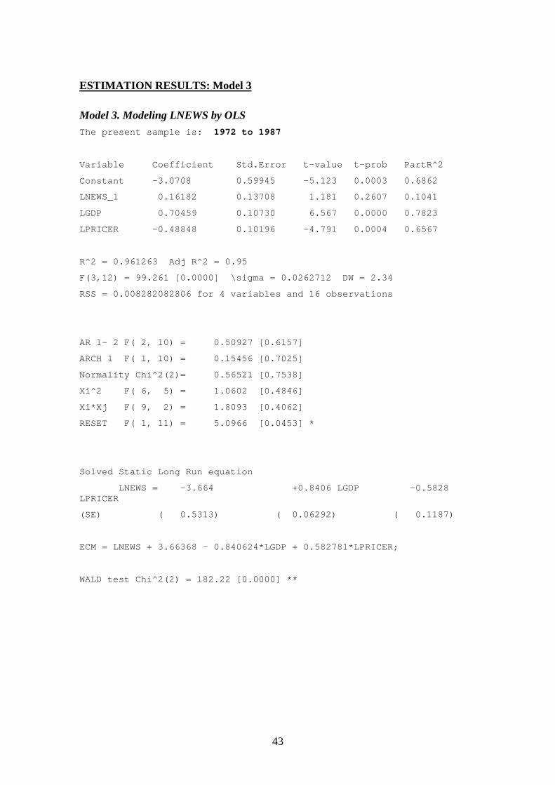
43
ESTIMATION RESULTS: Model 3
Model 3. Modeling LNEWS by OLSThe present sample is: 1972 to 1987
Variable Coefficient Std.Error t-value t-prob PartR^2
Constant -3.0708 0.59945 -5.123 0.0003 0.6862
LNEWS_1 0.16182 0.13708 1.181 0.2607 0.1041
LGDP 0.70459 0.10730 6.567 0.0000 0.7823
LPRICER -0.48848 0.10196 -4.791 0.0004 0.6567
R^2 = 0.961263 Adj R^2 = 0.95
F(3,12) = 99.261 [0.0000] \sigma = 0.0262712 DW = 2.34
RSS = 0.008282082806 for 4 variables and 16 observations
AR 1- 2 F( 2, 10) = 0.50927 [0.6157]
ARCH 1 F( 1, 10) = 0.15456 [0.7025]
Normality Chi^2(2)= 0.56521 [0.7538]
Xi^2 F( 6, 5) = 1.0602 [0.4846]
Xi*Xj F( 9, 2) = 1.8093 [0.4062]
RESET F( 1, 11) = 5.0966 [0.0453] *
Solved Static Long Run equation
LNEWS = -3.664 +0.8406 LGDP -0.5828LPRICER
(SE) ( 0.5313) ( 0.06292) ( 0.1187)
ECM = LNEWS + 3.66368 - 0.840624*LGDP + 0.582781*LPRICER;
WALD test Chi^2(2) = 182.22 [0.0000] **
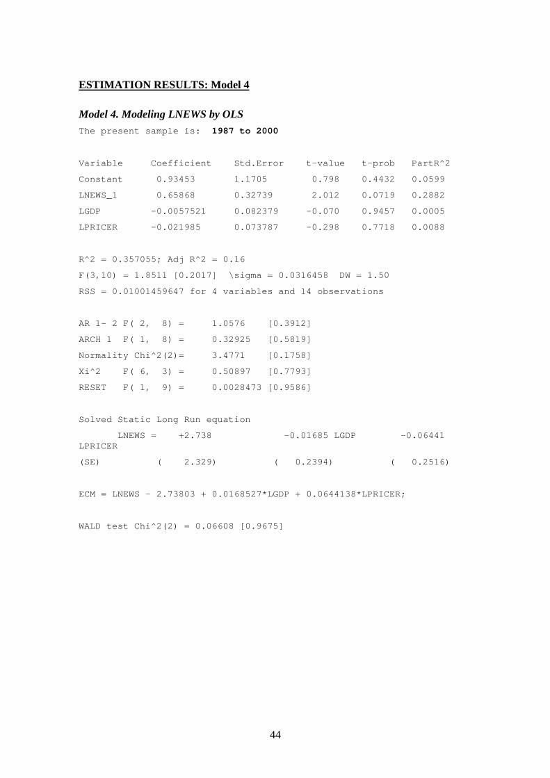
44
ESTIMATION RESULTS: Model 4
Model 4. Modeling LNEWS by OLSThe present sample is: 1987 to 2000
Variable Coefficient Std.Error t-value t-prob PartR^2
Constant 0.93453 1.1705 0.798 0.4432 0.0599
LNEWS_1 0.65868 0.32739 2.012 0.0719 0.2882
LGDP -0.0057521 0.082379 -0.070 0.9457 0.0005
LPRICER -0.021985 0.073787 -0.298 0.7718 0.0088
R^2 = 0.357055; Adj R^2 = 0.16
F(3,10) = 1.8511 [0.2017] \sigma = 0.0316458 DW = 1.50
RSS = 0.01001459647 for 4 variables and 14 observations
AR 1- 2 F( 2, 8) = 1.0576 [0.3912]
ARCH 1 F( 1, 8) = 0.32925 [0.5819]
Normality Chi^2(2)= 3.4771 [0.1758]
Xi^2 F( 6, 3) = 0.50897 [0.7793]
RESET F( 1, 9) = 0.0028473 [0.9586]
Solved Static Long Run equation
LNEWS = +2.738 -0.01685 LGDP -0.06441LPRICER
(SE) ( 2.329) ( 0.2394) ( 0.2516)
ECM = LNEWS - 2.73803 + 0.0168527*LGDP + 0.0644138*LPRICER;
WALD test Chi^2(2) = 0.06608 [0.9675]
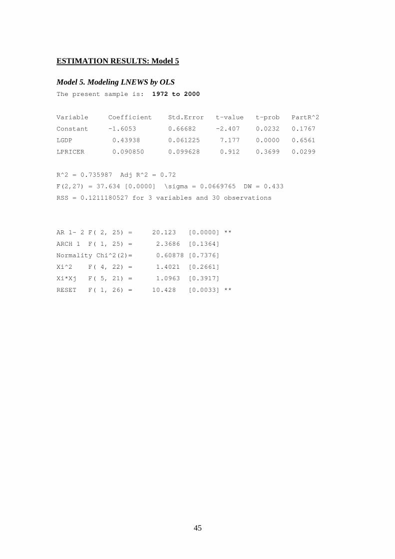
45
ESTIMATION RESULTS: Model 5
Model 5. Modeling LNEWS by OLSThe present sample is: 1972 to 2000
Variable Coefficient Std.Error t-value t-prob PartR^2
Constant -1.6053 0.66682 -2.407 0.0232 0.1767
LGDP 0.43938 0.061225 7.177 0.0000 0.6561
LPRICER 0.090850 0.099628 0.912 0.3699 0.0299
R^2 = 0.735987 Adj R^2 = 0.72
F(2,27) = 37.634 [0.0000] \sigma = 0.0669765 DW = 0.433
RSS = 0.1211180527 for 3 variables and 30 observations
AR 1- 2 F( 2, 25) = 20.123 [0.0000] **
ARCH 1 F( 1, 25) = 2.3686 [0.1364]
Normality Chi^2(2)= 0.60878 [0.7376]
Xi^2 F( 4, 22) = 1.4021 [0.2661]
Xi*Xj F( 5, 21) = 1.0963 [0.3917]
RESET F( 1, 26) = 10.428 [0.0033] **
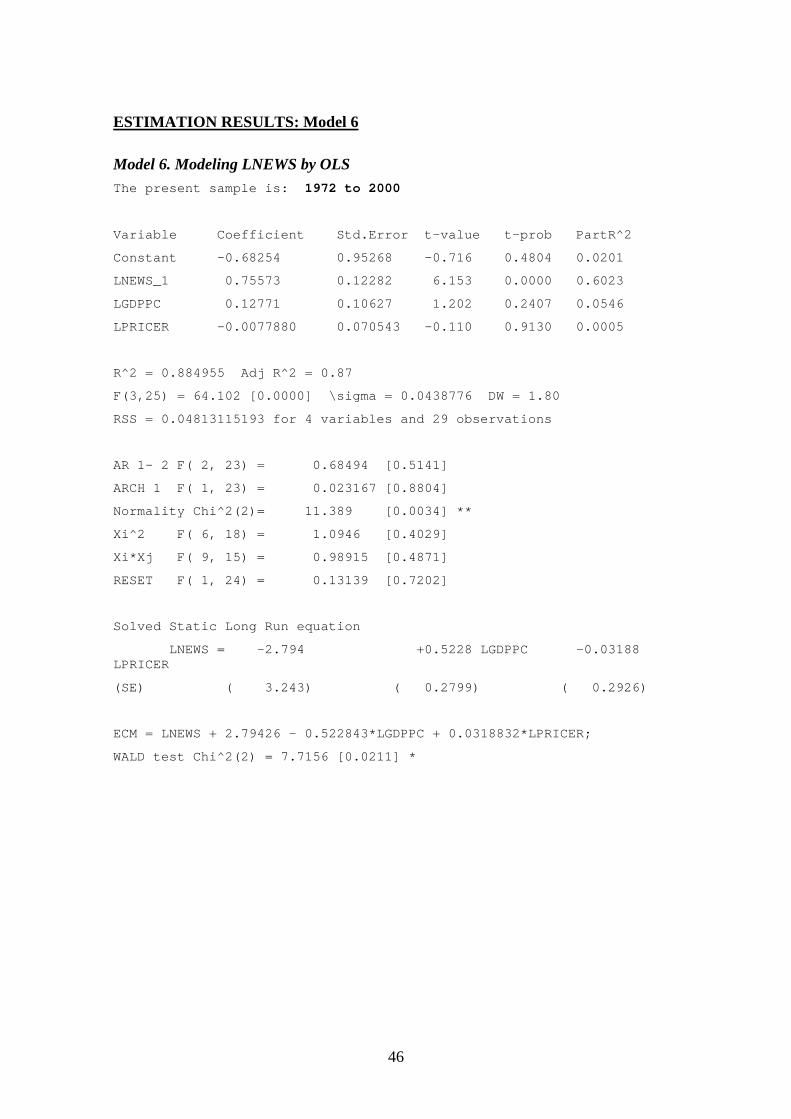
46
ESTIMATION RESULTS: Model 6
Model 6. Modeling LNEWS by OLSThe present sample is: 1972 to 2000
Variable Coefficient Std.Error t-value t-prob PartR^2
Constant -0.68254 0.95268 -0.716 0.4804 0.0201
LNEWS_1 0.75573 0.12282 6.153 0.0000 0.6023
LGDPPC 0.12771 0.10627 1.202 0.2407 0.0546
LPRICER -0.0077880 0.070543 -0.110 0.9130 0.0005
R^2 = 0.884955 Adj R^2 = 0.87
F(3,25) = 64.102 [0.0000] \sigma = 0.0438776 DW = 1.80
RSS = 0.04813115193 for 4 variables and 29 observations
AR 1- 2 F( 2, 23) = 0.68494 [0.5141]
ARCH 1 F( 1, 23) = 0.023167 [0.8804]
Normality Chi^2(2)= 11.389 [0.0034] **
Xi^2 F( 6, 18) = 1.0946 [0.4029]
Xi*Xj F( 9, 15) = 0.98915 [0.4871]
RESET F( 1, 24) = 0.13139 [0.7202]
Solved Static Long Run equation
LNEWS = -2.794 +0.5228 LGDPPC -0.03188LPRICER
(SE) ( 3.243) ( 0.2799) ( 0.2926)
ECM = LNEWS + 2.79426 - 0.522843*LGDPPC + 0.0318832*LPRICER;
WALD test Chi^2(2) = 7.7156 [0.0211] *
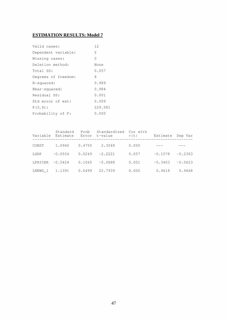
47
ESTIMATION RESULTS: Model 7
Valid cases: 12
Dependent variable: Y
Missing cases: 0
Deletion method: None
Total SS: 0.057
Degrees of freedom: 8
R-squared: 0.989
Rbar-squared: 0.984
Residual SS: 0.001
Std error of est: 0.009
F(3,8): 229.581
Probability of F: 0.000
Standard Prob Standardized Cor withVariable Estimate Error t-value >|t| Estimate Dep Var----------------------------------------------------------------------
CONST 1.0960 0.4755 2.3048 0.050 --- ---
LGDP -0.0554 0.0249 -2.2221 0.057 -0.1578 -0.2363
LPRICER -0.5424 0.1065 -5.0888 0.001 -0.3403 -0.0623
LNEWS_1 1.1391 0.0499 22.7939 0.000 0.9618 0.9668
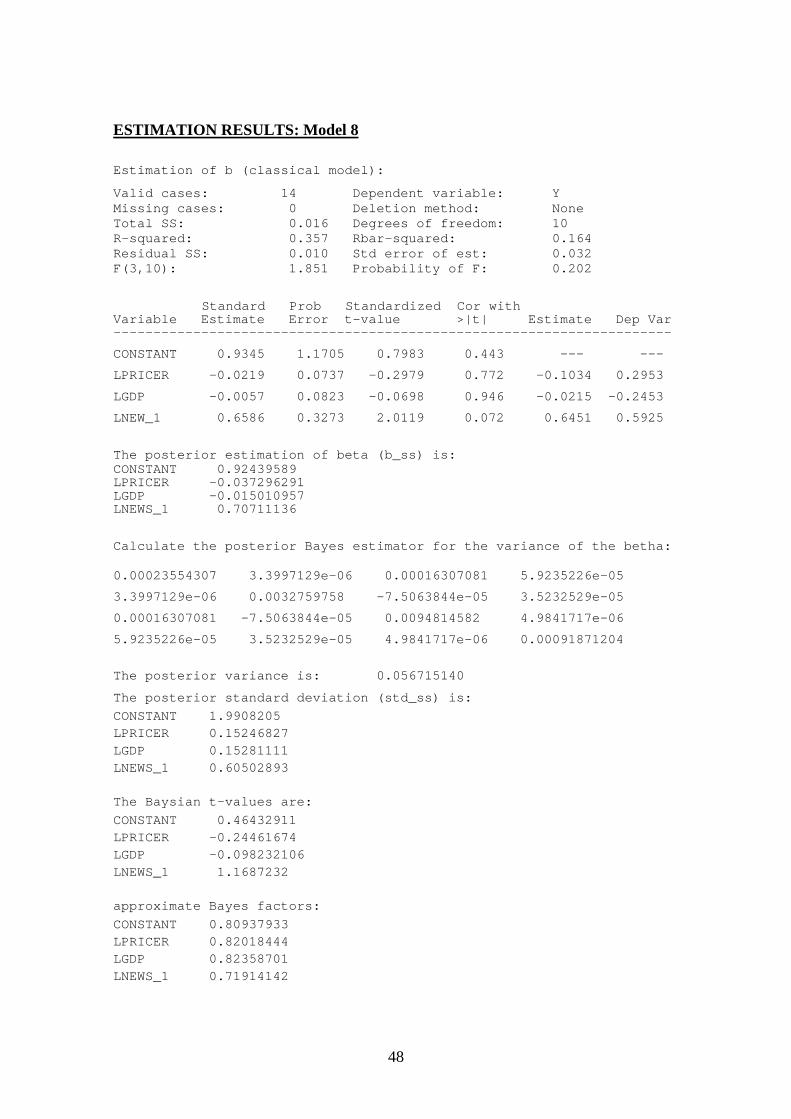
48
ESTIMATION RESULTS: Model 8
Estimation of b (classical model):
Valid cases: 14 Dependent variable: YMissing cases: 0 Deletion method: NoneTotal SS: 0.016 Degrees of freedom: 10R-squared: 0.357 Rbar-squared: 0.164Residual SS: 0.010 Std error of est: 0.032F(3,10): 1.851 Probability of F: 0.202
Standard Prob Standardized Cor withVariable Estimate Error t-value >|t| Estimate Dep Var----------------------------------------------------------------------
CONSTANT 0.9345 1.1705 0.7983 0.443 --- ---
LPRICER -0.0219 0.0737 -0.2979 0.772 -0.1034 0.2953
LGDP -0.0057 0.0823 -0.0698 0.946 -0.0215 -0.2453
LNEW_1 0.6586 0.3273 2.0119 0.072 0.6451 0.5925
The posterior estimation of beta (b_ss) is:CONSTANT 0.92439589LPRICER -0.037296291LGDP -0.015010957LNEWS_1 0.70711136
Calculate the posterior Bayes estimator for the variance of the betha:
0.00023554307 3.3997129e-06 0.00016307081 5.9235226e-05
3.3997129e-06 0.0032759758 -7.5063844e-05 3.5232529e-05
0.00016307081 -7.5063844e-05 0.0094814582 4.9841717e-06
5.9235226e-05 3.5232529e-05 4.9841717e-06 0.00091871204
The posterior variance is: 0.056715140
The posterior standard deviation (std_ss) is:
CONSTANT 1.9908205LPRICER 0.15246827LGDP 0.15281111LNEWS_1 0.60502893
The Baysian t-values are:
CONSTANT 0.46432911LPRICER -0.24461674LGDP -0.098232106LNEWS_1 1.1687232
approximate Bayes factors:
CONSTANT 0.80937933LPRICER 0.82018444LGDP 0.82358701LNEWS_1 0.71914142
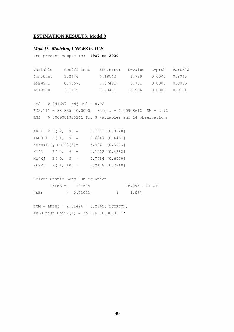
49
ESTIMATION RESULTS: Model 9
Model 9. Modeling LNEWS by OLSThe present sample is: 1987 to 2000
Variable Coefficient Std.Error t-value t-prob PartR^2
Constant 1.2476 0.18542 6.729 0.0000 0.8045
LNEWS_1 0.50575 0.074919 6.751 0.0000 0.8056
LCIRCCH 3.1119 0.29481 10.556 0.0000 0.9101
R^2 = 0.941697 Adj R^2 = 0.92
F(2,11) = 88.835 [0.0000] \sigma = 0.00908612 DW = 2.72
RSS = 0.0009081333261 for 3 variables and 14 observations
AR 1- 2 F( 2, 9) = 1.1373 [0.3628]
ARCH 1 F( 1, 9) = 0.6347 [0.4461]
Normality Chi^2(2)= 2.406 [0.3003]
Xi^2 F( 4, 6) = 1.1202 [0.4282]
Xi*Xj F( 5, 5) = 0.7784 [0.6050]
RESET F( 1, 10) = 1.2118 [0.2968]
Solved Static Long Run equation
LNEWS = +2.524 +6.296 LCIRCCH
(SE) ( 0.01021) ( 1.06)
ECM = LNEWS - 2.52426 - 6.29623*LCIRCCH;
WALD test Chi^2(1) = 35.276 [0.0000] **