1

IMPROVED OPTICAL FLOW ESTIMATION METHOD FOR

DEEPFAKE VIDEOS

Ali Bou Nassif*, Qassim Nasir, Manar Abu Talib, Omar Mohamed Gouda {anassif, nasir, mtalib, u19104867}@sharjah.ac.ae

University of Sharjah, Sharjah, UAE, Zip: 27272

Abstract

Creating deepfake multimedia, and especially deepfake videos, has become much easier these days due

to the availability of deepfake tools and the virtually unlimited numbers of face images found online.

Research and industry communities have dedicated time and resources to develop detection methods to

expose these fake videos. Although these detection methods have been developed over the past few

years, synthesis methods have also made progress, allowing for the production of deepfake videos that

are harder and harder to differentiate from real videos. This research paper proposes an improved optical

flow estimation-based method to detect and expose the discrepancies between video frames.

Augmentation and modification are used to improve the system’s overall accuracy. Furthermore, the

system is trained on Graphics Processing Units (GPUs) and Tensor Processing Units (TPUs) to explore

the effects and benefit of each type of hardware in deepfake detection. TPUs were found to have shorter

training times compared to the GPUs. VGG-16 is the best performing model when used as backbone for

the system, as it achieved around 82.0% detection accuracy when trained on GPUs and 71.34% accuracy

on TPUs.

Keywords: Deepfake; Optical flow; Tensor Processing Units (TPU); GPU; Convolutional Neural

Networks (CNNs)

* Corresponding Author: Ali Bou Nassif

2

1. Introduction

Deepfake multimedia (manipulated images, video and audio) have grown to become more and

more of a threat to public opinion [1]. These fake multimedia are easily spread all over the world

thanks to social media platforms that connect people with a click of a button [2]. Seeing a

manipulated deepfake video of a public figure can alter a citizen’s opinions or political stance within

seconds. The term deepfake refers to manipulated multimedia generated using Artificial

Intelligence (AI) based tools [3].

The most disruptive type of deepfake is a manipulated video in which a target person’s face is

replaced by another face, while keeping the target’s facial expression [4]. Although these generated

videos can be very realistic and hard to detect, they are very easy to create. The availability of a

wide variety of images and online videos has helped to provide enough data to create a huge number

of fake videos. Anyone can generate these videos by combining the data available with free and

open-source tools like FaceApp [5]. Some positive applications of deepfake tools can be seen in

movie productions, photography and even video games [6]. However, deepfake technology has

been infamously used for malicious purposes, like creating fake news. To address the problem of

the malicious use of deepfake technology, the research and commercial communities have

developed a number of methods to verify the integrity of multimedia files and to detect deepfake

videos. Most of the methods attempt to detect deepfake videos by analyzing pixel values [7,8].

These methods rely on the visual artifacts created while placing the fake face on the target face.

The artifacts are significant because they represent missing information that the deep neural

network did not see in the training data (e.g. teeth), sometimes because it is hidden behind another

object (e.g. hair strand). The deep network cannot estimate the information and therefore assigns it

a lower quality in the deepfake version, or even creates holes in these parts [9].

3

Figure 1- Difference between real (top) and fake (bottom) frames passed to optical flow estimator.

However, the situation has changed considerably with recent developments in deep learning

networks. These artifacts are now less common than before and can no longer be seen in the new

videos [10]. On the other hand, extracting other useful data from the video’s spatial and temporal

information has proved to be effective. The estimated pattern of apparent motion over the length of

time is called optical flow. This paper discusses how optical flow information can be exploited to

detect anomalies in manipulated videos.

This research paper presents an effective technique to detect deepfake videos based on optical

flow estimation. A sequence-based approach is used to detect the temporal discrepancies of a video.

Inter-frame correlations are extracted using optical flow and are then used as input in a

Convolutional Neural Network (CNN) classifier. An example of applying optical flow estimation

on real and fake frames can be seen in Figure 1. The proposed method is investigated using multiple

neural networks to form the backbone of the system. TPUs are used to train another version of the

system and a comparison is presented in this research. Furthermore, multiple methods of deepfake

detection are tested on various datasets. Experiments are conducted using fine-tuning and

augmentation techniques in order to improve the system. As this is the first work that uses TPU as

training hardware to detect deepfakes, the research community can build and modify this work to

explore TPU capabilities in detection methods. Furthermore, optical flow information in deepfakes

has not yet been fully explored. This method can be utilized to build new detection methods.

4

The system achieves detection accuracy of 82% when trained on GPU and has been trained and

tested on multiple datasets. Multiple CNN models were tested to determine what should be used as

a backbone for this system, and the VGG family had the best results. Augmentations were

implemented to improve overall accuracy, but none of the augmentations were found to improve

accuracy.

This paper has been laid out as follows: the related work on deepfake detection techniques is

discussed in Section 2, while Section 3 presents background information related to the detection

technique presented in this paper. Section 4 describes the methodology and modifications proposed

in this paper to improve the overall accuracy of the system. Section 5 discusses the preparations

and preprocessing done before the experiments, followed by an examination of the experiments

conducted and their results in Section 6. Finally, Section 7 draws conclusions.

2. Related Work

A brief overview of related research work is discussed in this section.

Matern et al [9] proposed a method that focused on exploiting visual artifacts in generated and

manipulated faces. The authors focused on the three most notable artifacts in the deployed detection

method. The first artifact is the discoloration of the eyes. When a face generation algorithm creates

a new face, the data points are interpolated between faces to find a plausible result. The algorithm

tries to find two eyes from different faces that are matching in color. Utilizing the knowledge

obtained by observing the fake data, the authors created their dataset from ProGan [11] and Glow

[12] face generation datasets and generated deepfake and face2face [13] images using data from

the Celeb-A dataset. Although the dataset used was limited to a small number, the results, as seen

in Table 1, are very promising in this method.

Qi et al [6] proposed an effective detection method utilizing remote visual

photoplethysmography (PPG). Capturing and comparing the heartbeat rhythms of both the real and

fake faces is the key idea of this method. The PPG monitors small changes of skin color caused by

5

the blood moving through the face [14]. Using this information, PPG calculates an accurate

estimation of the person’s heartbeat. The general concept assumes that fake faces should have a

disrupted or non-existent heartbeat rhythm compared to the normal rhythms produced by real

videos. The authors have done extensive testing on FaceForensics++ [7] and DFDC [15] datasets

to demonstrate not only the effectiveness but also the generality of this method on different

deepfake techniques.

Guera et al [16] proposed a temporal method to detect deepfake videos. The system utilizes CNN

to extract features from a video on the frame-level. The extracted features are then used to train a

recurrent neural network (RNN). The network learns to classify if the input video has been altered

or not. The key advantage of this method is that it considers a sequence of frames when detecting

deepfake videos. The authors chose to train the system on the HOHA dataset [17] because this

dataset contains a realistic set of sequence samples from famous movies from which most deepfake

videos are generated.

Amerini et al [18] proposed a detection method exploiting the discrepancies in optical flow in

fake faces as compared to real ones. The system transfers extracted cropped faces from video to

PWC-Net [19], an optical flow CNN predictor. The authors conducted their tests on two well-

known networks: VGG-16 [20] and ResNet50 [21]. Transfer learning was utilized to reduce training

time and improve system accuracy. FaceForensics++ [7] uses multiple manipulation methods that

the authors used in their tests. The three methods used are deepfakes, face2face, and face swap.

Only the binary detection accuracy of face2face was shared in the research paper, with VGG-16

and ResNet50 detecting AI-generated faces with an accuracy of 81.61% and 75.46% respectively.

Jeon et al [8] proposed a light-weight robust fine-tuning neural network-based classifier capable

of detecting fake faces. This system excels in its use of existing classification networks and its ease

in fine-tuning these networks. The authors aim to reuse popular pre-trained models and fine-tune

them with new images to increase detection accuracy. The system takes the cropped face images

from the videos and transfers them to the backbone model, which is trained on a large number of

6

images (78,000 images training/validation). The preliminary results show a substantial

improvement in the accuracy of the models, with around 2 to 3% on the Xception [22] models and

33 to 40% for SqueezeNet models. The datasets used in this research paper included PGGAN [23],

deepfakes, and face2face from the FaceForensics++ [7] dataset. The proposed augmentations and

fine-tuning were applied only to the raw pixels of the image. However, discrepancies in the raw

images, as mentioned before, are decreasing and may disappear entirely in the near future. Instead,

implementing these techniques on the networks that analyze optical flow may increase the

efficiency of these networks.

To overcome these limitations, we propose a system that is based on exploiting optical flow

inconsistencies in video to detect deepfake videos using pre-trained CNNs and augmentations.

Table 1 shows a comparison between the various deepfake detection methods discussed in this

section, including the method proposed in this work.

The main contribution of this work can be summarized as follows:

• Improved accuracy: The proposed method is more accurate overall than other methods

that utilize optical flow.

• Detecting multiple deepfake techniques: Tests are conducted on several deepfake

techniques including Deepfakes and face2face.

• Experimenting with fine-tuning techniques: New augmentation techniques proposed by

Jeon et al [8] are implemented with the proposed method to improve accuracy in this paper.

• Using several models as a backbone: Further experiments on several networks are

conducted and compared to achieve the best accuracy out of all networks.

• Detecting multiple datasets: Several deepfake datasets are used in this work and compared.

• Using TPU and GPU on the proposed method: The system is also trained on TPUs and

compared with the GPU results as well.

7

Table 1: Summary of related work in deepfake detection

(*) means all types of manipulation methods were used in the paper.

Research Paper Year Method Domain Datasets Hardware Accuracy

DeepRhythm

[6] 2020

Heartbeat

rhythms using

PPG with

attention

network

Dual-

spatial-

temporal

FF++*

DFDC GPU

Accuracy:

98.0%

FDFtNet [8] 2020

Augmentation

of pretrained

CNN

Pixel-

Level

detection

PGGAN,

FF++ -

Deepfake,

FF++ -

Face2Face

GPU

AUROC:

0.994

Accuracy:

97.02%

Face X-Ray

[24] 2020

Detection of

blending

boundaries in

the image

Pixel-

Level

detection

FF++*

DFDC

DFD

Celeb-DF

GPU AUC: 95.4

Visual

Artifacts [9] 2019

Visual

artifacts

(eyes, teeth

and nose &

face border)

Pixel-

Level

detection

Glow,

ProGan,

celeb-A GPU

AUROC:

0.866

Optical Flow

[18] 2019

Inter-frame

correlations

using optical

flow

Spatio-

temporal FF++ -

Face2Face GPU

Accuracy:

81.61%

Recurrent

Neural

Networks [16]

2019

Recurrent

Neural

Network

Spatio-

temporal HOHA GPU

Accuracy:

97.1%

FF++ - Xception

[7] 2019

CNN-based

Image

classification

Pixel-

Level

detection

FF++*

GPU

Accuracy:

96.36%

Eye Blinking

[25] 2018

Discrepancies

in eye

blinking

across the

frames

Spatio-

temporal CEW GPU

AUROC:

0.98

This research

paper 2020

Inter-frame

correlations

using optical

flow

Spatio-

temporal

FF++ -

Deepfake,

FF++ -

Face2Face

Celeb-DF,

DFDC

GPU, TPU

AUROC:

0.879

Accuracy:

82%

8

3. Background

This section contains a brief overview of the inner mechanisms of deepfake and its types.

Furthermore, different deepfake datasets are briefly discussed and compared based on dataset size

and techniques used. An introduction about optical flow along with a short description of the most

effective method used in this paper is also presented.

3.1 Deepfake

The power of AI has been harnessed to generate forged visual and audio content and new

methods are continually being introduced. Most of these methods produce realistic video or audio

segments that are difficult to recognize. The ability to produce such high-quality forensics is the

result of an advancement in Generative Adversarial Networks (GANs) and Autoencoders (AEs)

[26].

GANs enhancements led to major improvements in image generation and video prediction. The

fundamental principle of GANs is that a generator and a discriminator are trained concurrently. The

generator produces fake reconstruction samples by using input from a random source [26]. The

technique of the GAN is to make the generated reconstructions appear closer to a natural image.

This is done by moving these reconstructions towards high probability regions in search space that

contains photo-realistic images. The discriminator is trained to distinguish real samples of a dataset

from forged reconstructions. The training of the discriminator ends when convergence occurs,

which is done when the distribution produced by the generator matches the data distribution [7]. In

more advanced approaches for deepfakes, GANs can be used along with Autoencoders (AEs) to

generate fake images and videos.

Various methods are being used in deepfake generation techniques. They can be classified

according to the type of media forged. Deepfake types can be classified as shown in Table 2.

9

Table 2 - Types of deepfake manipulation

Type Photo Audio Video

Description

This type

includes

manipulations

done on images,

i.e.: to generate a

non-existent face

image.

This type includes any type of

manipulation done on audio

records, i.e.: impersonating or

changing a person’s voice.

This type includes

manipulations done on

videos.

Class • Face and

Body swapping.

• Impersonating person’s

voice.

• Changing a person’s voice.

• Speech to text usage to

change part of audio to a

specific text.

• Face-swapping.

• Face-morphing.

• Full body

puppetry.

Example • FaceApp [5].

• Synthesizing Obama:

Learning lip sync from

audio [27].

• Waveglow [28]

• Face2Face [13]

• Pose Transfer [29]

3.2 Deepfake Datasets

As mentioned in the previous section, there are different categories of DeepFake manipulations.

In this section, datasets related to face swapping and facial expression manipulation are presented.

They are also used in this work as shown in Table 3.

Table 3 - Deepfake datasets

Dataset Year Size (videos) Techniques

FF++ [7] 2019 1000 real 7000

fake (all

techniques)

Deepfakes, Face2face,

Face swap, NeuralTextures

Celeb-DF v2

[10]

2020 590 / 5,639 Deepfakes

DFDC [15] 2020 19,154 / 100,000 Deepfakes

FaceForensics++ [7] is one of the most utilized datasets in deepfakes. This dataset is generated

from 1000 pristine videos available on Internet. Many manipulation techniques have been applied

to generate fake videos from these 1000 videos. The techniques used can be classified into two

10

categories: computer graphics-based and two-learning based approaches. Computer graphics-based

approaches include such techniques as Face2Face and FaceSwap. Examples of the two-learning

based approaches include DeepFakes and NeuralTextures. One of the features of the dataset is that

it supports a variety of video qualities, which is an important factor in video forensics and the

deepfakes paradigm.

Celeb-DF [10] is a large-scale video dataset that consists of 2 million frames that correspond to

5,693 deepfake videos. This dataset is characterized by diversity in the gender, age and ethnic group

of its subjects, as its videos are sourced from YouTube. Using an enhanced deepfake synthesis

method, fake videos are generated from the source videos. The recently introduced Celeb-DF v2

overcomes the shortcoming of the original version of the dataset, as it has significantly fewer

notable visual artifacts.

A new challenging dataset that has been introduced lately is Deepfake Detection Challenge

dataset (DFDC) [15]. This dataset consists of more than 100,000 videos that takes into consideration

variability in gender, skin tone, age, varying lighting conditions and head poses. Currently, DFDC

dataset is the largest publicly available face swap video dataset. The forgery videos are generated

using several techniques including deepfake, GAN-based and non-learned methods.

3.3 Optical flow

One of the key problems in computer vision is optical flow estimation. However, this field is

making steady progress, which can be seen in the current methods on the Middlebury optical flow

benchmark [30]. Optical flow estimation is the estimation of the displacement between two images

and is conducted at the pixel level. Multiple approaches were introduced to make this type of

estimation conclusive. Horn and Schunck introduced the variational approach, in which brightness

constancy and spatial smoothness are coupled and passed to an energy function [31]. However,

using energy functions is computationally expensive, especially for real-time applications. To

11

overcome this problem, CNNs are adopted to maximize speed and minimize cost. One of the top-

performing methods that uses CNNs is PWC-Net [19].

Figure 2 - PWC-Net Network Architecture [19]

PWC-Net, as shown in Figure 2, utilizes pyramid, wrapping and cost volume processing along

with CNN, building a feature pyramid from the two input images. Unlike approaches like FlowNet

[32], which uses fixed-image pyramids, PWC-Net employs learnable feature pyramids [19]. A cost

volume is constructed at the top level of the pyramid by comparing the features of a pixel in the

first image with the corresponding features in the second image. The cost volume is constructed

using a small search range, as the topmost levels have small spatial resolution. The cost volume and

features of the first image are passed to a CNN to estimate flow at the top level. PWC-Net passes

to the next level the estimated flow that has been upsampled and rescaled [19].

PWC-Net warps features of the second image toward the first using the upsampled flow at the

second level from the top. Using the features of the first image and the warped features, PWC-Net

constructs a cost volume. This process repeats until the desired level is reached [19].

4. Methodology

In this section, the proposed method is described. The method’s overall architecture is presented

in Figure 3. The architecture uses several different approaches to improve the system’s overall

accuracy. GPU-based, TPU-based and augmented approaches of the proposed system are presented.

12

4.1 Proposed Architecture

As presented in Figure 3, the proposed system starts with a preprocessing stage in which the

person’s face is extracted before analyzing the video. In this preprocessing stage, the frames of the

video are extracted and saved on the system disk. The extracted frames are much larger in size than

the source video. Furthermore, in this system, the interest region is the face. The frames are

therefore passed to MTCNN [33], which detects the faces in the frames, and then to OpenCV [34],

which crops the frames to contain only faces and ensures that the frames are all a fixed size.

The cropped frames are then passed to PWC-Net [19], which will process the frames in

chronological order and extract the movement between the scene and the observer, which is done

between two consecutive frames 𝑓(𝑡) and 𝑓(𝑡 + 1). The former process is called Optical flow.

The information generated from this process is in a vector field format. Each value has a magnitude,

which refers to the amount of motion in that pixel or point, and the direction of the scene’s motion

between these two frames.

Figure 3 - Overall proposed system architecture

Each optical flow vector is visualized and presented as an RGB image. These frames are called

optical flow frames or images. The pixel color represents the angle between the flow vector and the

horizontal axis, while colour saturation represents the intensity of the motion in this pixel. This step

13

was taken in order to save training time and reusing the information obtained by the existing

implementations and pre-trained networks trained on raw RGB images.

The optical flow images are then passed to Detection CNN, which uses a pre-trained CNN as a

backbone. Transfer learning is adopted for this approach, as these networks are already trained on

RGB images. Exploiting the knowledge they retain; additional training is conducted with three

dense layers to fine-tune the network on the optical flow images.

The hypothesis for this architecture is that the optical flow should detect and show any

discrepancies in motion that were added or synthesized into the frame. These differences should be

noticeable when compared to the real parts of the frames that were created by the camera. The

regions of interest are the eyes, the mouth, and the face outline. These regions are most likely to

contain the said discrepancies, as deepfake synthesis algorithms struggle the most with these

regions.

The results of the Detection CNN are evaluated using the test dataset, which is a subset of the

same dataset used in training. This dataset was not used in the training phase of the model.

4.2 GPU Approach

The basic structure of the GPU approach is shown in Figure 4. The overall architecture of this

approach replaces the Detection CNN with a CNN that was pre-trained using a GPU. Multiple

networks have been tested, including but not limited to VGG16 [20] and Xception [22].

The network uses the original top layer of the network. For example, VGG-16 uses 224 x 224

image size as input. Then, using the Keras [35] function Image generator, the images are scaled to

the correct size for the network. As Keras retains all of the weights taken from Imagenet [36], only

the last three layers plus the dense ones are kept trainable. All other layers become untrainable.

Finally, the last dense layer is switched with a softmax dense layer that categorizes the frames as

fake or real. The rest of the training settings are discussed in the next section.

14

Figure 4 - GPU architecture of the system.

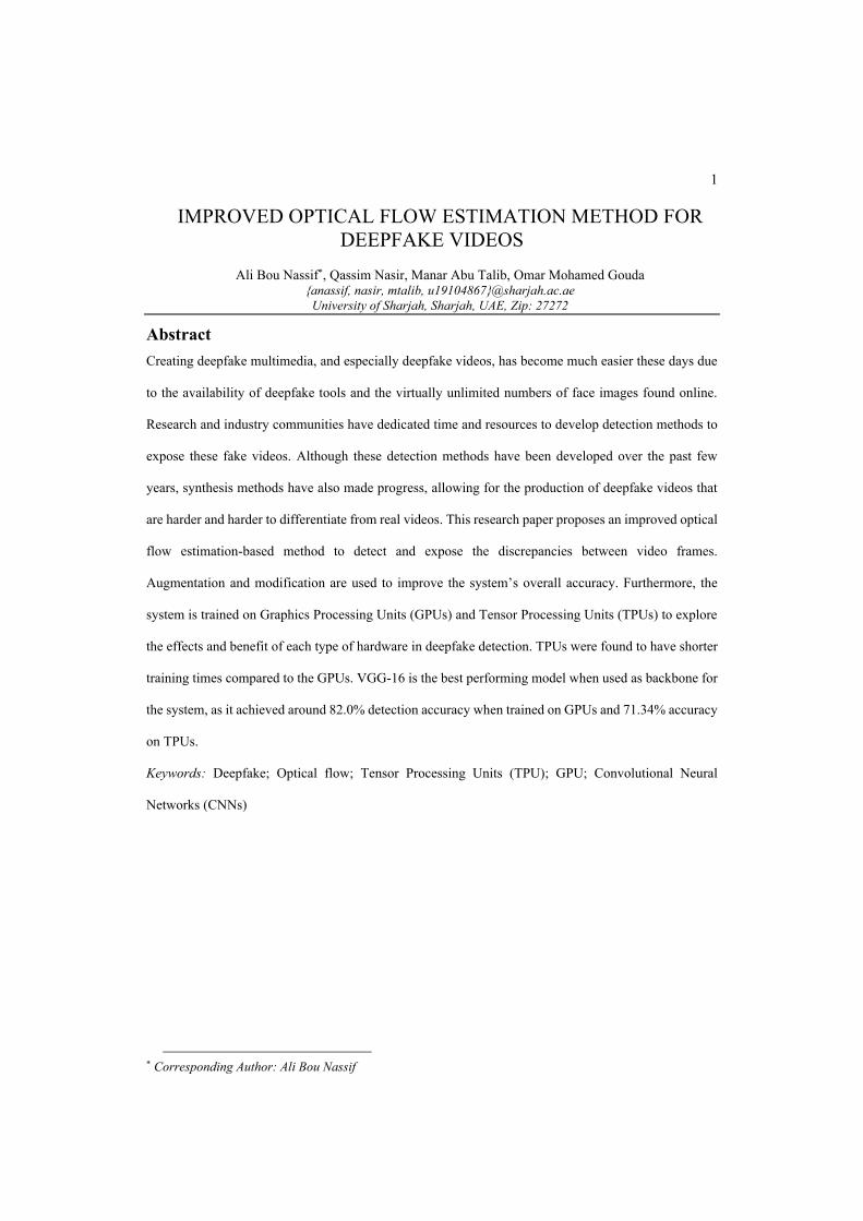
4.3 Augmentations and Fine-Tuning Approach

Jeon et al [8] proposed a new self-attention module for image classifications called Fine-Tune

Transformer. It was used with MobileNet Block to improve existing networks that were trained on

deepfake images. Our methods of implementing this fine-tuning method on the proposed design is

explained in this section, along with multiple augmentations.

In order to apply the fine-tuning method as it was mentioned in the paper and as shown in Figure

5a, we take the pre-trained GPU approach CNN as the backbone and pass it to the MobileNet block.

At the same time, the FFT block is trained on the same dataset as the MobileNet. All other

parameters are maintained exactly as in the GPU approach. Another augmentation as shown in

Figure 5b is to train the FFT alongside the CNN, as this may increase the accuracy of the entire

system. Augmentations 3 and 4 are very similar, placing different blocks after the CNN. MobileNet

block is used in Augmentation 3 and FTT in Augmentation 4 as shown in Figure 5c and Figure 5d,

respectively.

15

Figure 5 – Four different augmentations (a) Augmentation 1: applying the proposed

augmentation by Jeon et al (b) Augmentation 2: Training the FFT block alongside the CNN.

(c) Augmentation 3: Attaching MobileNet block at the end of the CNN. (d) Augmentation 4:

Attaching FTT block at the end of the CNN.

4.4 TPU Approach

The Tensor Processing Unit (TPU) is a custom ASIC-based accelerator. It has been deployed in

datacenters since 2015, but access for academic purposes was only given in 2018. In most neural

networks, TPUs speed up the inference stage, which is a crucial stage in which models are used to

infer or predict the testing sample.

The brain of the TPU has a 65,536 8-bit Multiplier Accumulator (MAC) matrix unit with

throughput that peaks at 92 TeraOps/second (TOPS) and with on-chip memory that is software-

(a)

(b)

(c) (d)

16

managed at 28 megabytes [37]. These specifications allow TPUs to handle a large number of data

that GPUs cannot handle and still be extremely fast. Nevertheless, TPUs requires extra effort from

the programmers to create a working model that can run seamlessly on these units.

Figure 6 - Basic architecture for the TPU approach

Kaggle platform offers the latest TPU v3 for academic purposes. The proposed model is adjusted,

as seen in Figure 6, to work on TPUs seamlessly. TPUs require image data to be in TFRecord

format, which converts the images into binary string along with their label. In this case, the image

size is fixed, and a custom data generator is used to read the binary sequence and convert it back

into an image. The data is distributed over 8 TPUs and the result is combined to enhance accuracy.

5. Preparations and Preprocessing

This section examines the preparations and preprocessing necessary before the experiments are

conducted.

5.1 Extraction and Filtering

For each dataset used in this paper, frames of each video were extracted with python code using

OpenCV [34]. The frames were then cropped by MTCNN [33] so that each image was of a fixed

size and contained only the subject’s face, before transferring the images to the optical flow

17

estimator. The images are first filtered manually, as the sequence of frames is very important in the

optical flow extraction step.

Sorting by size is a simple method used to find any images that do not belong in a given sequence.

Images with similar pixel values and density are more likely to have similar size, and are therefore

grouped together. Any foreign or unwanted frames are also grouped together, as they have different

characteristics. If the unwanted frames do not affect the sequence, the frames are deleted. However,

if they do affect the sequence, the video is either re-run through the MTCNN with a different

threshold or removed entirely.

After the filter is applied, the frames are passed into a PWC-Net [19] optical flow estimator. This

estimator works only on two frames at a time, given that is it provided two text lists containing the

frames to be used. Therefore, the image fetch code used in FlowNet2 [38] is used to automate the

process by providing the folder that contains the images. The number of frames transferred to the

estimator should be double the number used for the dataset. The estimator extracts data from two

consecutive frames, thereby cutting the number of produced images in half.

As mentioned before, for the TPU approach, the images should be in TFRecord format. The

images were converted to binary string and the label of the image into int32. Afterwards, the data

are put in a list and divided into batches of 2071 per TFRecord.

5.2 Training Settings

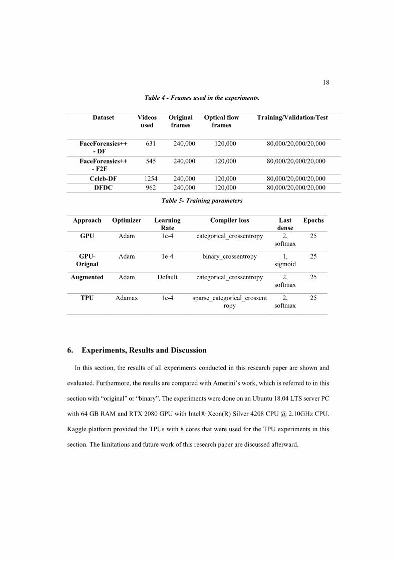
The following tables show the training settings used in tests and experimentations. Table 4 shows

the number of frames used, which is 120,000 optical flow images divided into 80-20-20 ratios.

Further down, Table 5 shows the parameters used for each model in detail.

18

Table 4 - Frames used in the experiments.

Dataset Videos

used

Original

frames

Optical flow

frames

Training/Validation/Test

FaceForensics++

- DF

631 240,000 120,000 80,000/20,000/20,000

FaceForensics++

- F2F

545 240,000 120,000 80,000/20,000/20,000

Celeb-DF 1254 240,000 120,000 80,000/20,000/20,000

DFDC 962 240,000 120,000 80,000/20,000/20,000

Table 5- Training parameters

Approach Optimizer Learning

Rate

Compiler loss Last

dense

Epochs

GPU Adam 1e-4 categorical_crossentropy 2,

softmax

25

GPU-

Orignal

Adam 1e-4 binary_crossentropy 1,

sigmoid

25

Augmented Adam Default categorical_crossentropy 2,

softmax

25

TPU Adamax 1e-4 sparse_categorical_crossent

ropy

2,

softmax

25

6. Experiments, Results and Discussion

In this section, the results of all experiments conducted in this research paper are shown and

evaluated. Furthermore, the results are compared with Amerini’s work, which is referred to in this

section with “original” or “binary”. The experiments were done on an Ubuntu 18.04 LTS server PC

with 64 GB RAM and RTX 2080 GPU with Intel® Xeon(R) Silver 4208 CPU @ 2.10GHz CPU.

Kaggle platform provided the TPUs with 8 cores that were used for the TPU experiments in this

section. The limitations and future work of this research paper are discussed afterward.

19

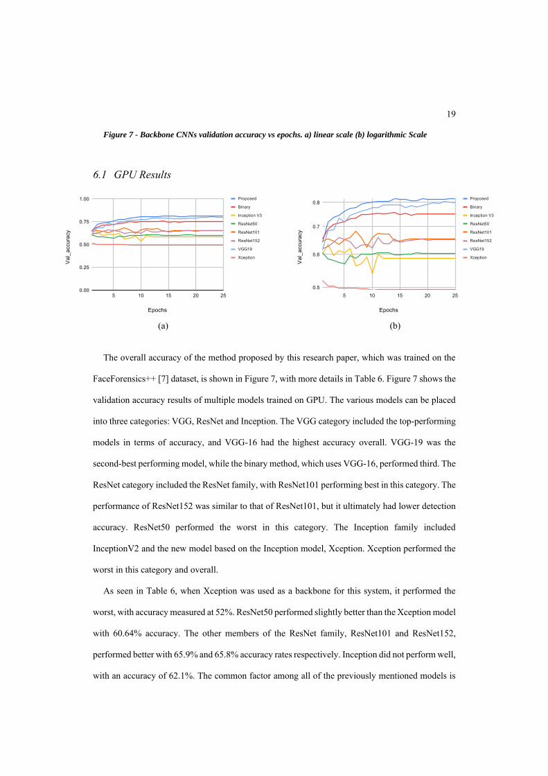
Figure 7 - Backbone CNNs validation accuracy vs epochs. a) linear scale (b) logarithmic Scale

6.1 GPU Results

The overall accuracy of the method proposed by this research paper, which was trained on the

FaceForensics++ [7] dataset, is shown in Figure 7, with more details in Table 6. Figure 7 shows the

validation accuracy results of multiple models trained on GPU. The various models can be placed

into three categories: VGG, ResNet and Inception. The VGG category included the top-performing

models in terms of accuracy, and VGG-16 had the highest accuracy overall. VGG-19 was the

second-best performing model, while the binary method, which uses VGG-16, performed third. The

ResNet category included the ResNet family, with ResNet101 performing best in this category. The

performance of ResNet152 was similar to that of ResNet101, but it ultimately had lower detection

accuracy. ResNet50 performed the worst in this category. The Inception family included

InceptionV2 and the new model based on the Inception model, Xception. Xception performed the

worst in this category and overall.

As seen in Table 6, when Xception was used as a backbone for this system, it performed the

worst, with accuracy measured at 52%. ResNet50 performed slightly better than the Xception model

with 60.64% accuracy. The other members of the ResNet family, ResNet101 and ResNet152,

performed better with 65.9% and 65.8% accuracy rates respectively. Inception did not perform well,

with an accuracy of 62.1%. The common factor among all of the previously mentioned models is

(a)

(b)

20

that all of them use a depth-wise separator convolution layer in their model. This layer’s

counterpart, the depth-wise convolution layer, is used in the VGG family. The original method

proposed by Amerini used binary classification and achieved 75.27% accuracy in detecting

deepfake images from the FF++ dataset. The second-best performance was achieved by the VGG-

19 model, with 80.1% accuracy. VGG-16 performed the best, with 82.0% accuracy, and was the

third-fastest model out of all tested models.

Figure 8 shows the accuracy results of the best performing model, which is VGG-16, trained on

different datasets and compared with the original method trained on the same datasets. Table 7

presents more details of the same test.

Table 6 - Backbone CNNs accuracy comparison. Values in bold are the best values in each category.

Model Time per

epoch

Total time Accuracy

Inception V3 [39] 800 secs 335 mins 62.1 %

ResNet 50 [21] 77 secs 33 mins 60.64 %

ResNet 101 [21] 1207 secs 507 mins 65.89 %

ResNet 152 [21] 1994 secs 839 mins 65.79 %

Xception [22] 633 secs 264 mins 52.0 %

VGG-19 698 secs 294 mins 80.1 %

VGG-16 Binary

(Amirini’s) [18]

446 secs 187 mins 75.27 %

VGG-16

(Proposed)

440 secs 183 mins 82.0 %

(a)

(b)

Figure 8 - Accuracy comparison between the proposed and the original trained on different datasets. a)

linear scale (b) logarithmic Scale

21

The proposed model attained much higher accuracy than the original method with minimal

modifications. The original method performed binary classification and used a fully connected

sigmoid output layer. The simple modification of using the categorical classification and softmax

output layer improved its accuracy. Another modification in the model was the input image size.

The original work used 300x300 images that were scaled down to 224x224. Using 130x130 images

and scaling them up to 224x224 also helped increase the accuracy of the model.

Table 7 - Dataset evaluation on proposed vs original. The highlighted values in bold are the best

performing for each dataset.

Model Dataset Accuracy Overall

accuracy

Proposed FaceForensics++ - DF 82.0 % 66.780%

FaceForensics++ - F2f 69.67%

Celeb-DF v2 74.24 %

DFDC 61.25 %

Original [18] FaceForensics++ - DF 75.27 % 63.435%

FaceForensics++ - F2f 67.37 %

Celeb-DF v2 50.0 %

DFDC 61.1 %

Table 8 shows the cross-validated results of the best performing model, which is the VGG-16

model, on four different datasets. The datasets include FaceForensics++ Deepfake and Face2Face,

DFDC, and Celeb-DF. The results are shared in Area Under the Receiver Operating Curve

(AUROC). The curve shows the trade-off between the false positive rate (FPR) and the true positive

rate (TPR) across different decision thresholds. The table shows that each model best detects the

dataset that was used in training. Overall, the model trained on FaceForensics++ Deepfake dataset

performed the best, at around 66.78% accuracy.

22

Table 8 - Accuracy comparison of the VGG-16 model trained and tested on different datasets. The values

in bold are the best performing for each dataset.

Validation

Trained FF++ - Deepfake

FF++ -

Face2Face DFDC Celeb-DF Overall

FF++ -

Deepfake

AUROC:0.878556 AUROC:0.710618 AUROC:0.521114 AUROC:0.528509 0.6276

Acc: 0.81995 Acc: 0.6478 Acc: 0.5184 Acc: 0.5241

FF++ -

Face2Face

AUROC:

0.766970

AUROC:

0.764427

AUROC:

0.480113

AUROC:

0.531422 0.6001

Acc: 0.6913 Acc: 0.69675 Acc: 0.4859 Acc: 0.52645

DFDC

AUROC:

0.519190

AUROC:

0.476737

AUROC:

0.650156

AUROC:

0.476790 0.5226

Acc: 0.5142 Acc: 0.48485 Acc: 0.61225 Acc: 0.4792

CelebDF

AUROC:

0.529061

AUROC:

0.529152

AUROC:

0.464086

AUROC:

0.806833 0.5650

Acc: 0.525 Acc: 0.5185 Acc: 0.4742 Acc: 0.74245

Figure 9 shows the comparison between the best performing GPU and other models trained on

the TPU. Similar to the GPU training results, three clear categorizes for the models can be seen in

the graph. The only model that deviated from its category was VGG-19, which performed much

worse than VGG-16. The accuracy of the VGG-16 GPU exceeded the same model’s TPU accuracy

by 12%. However, the speed that training was completed on TPU was phenomenal: around eight

times faster than the GPU training periods, as shown in Table 9 in the next section.

(a)

(b)

Figure 9 – Comparison between the best performing GPU and other models trained on the TPU. (a)

linear scale (b) logarithmic scale

23

6.2 TPU Results

As stated above, training was completed on TPU around eight times faster than on GPU.

Furthermore, there was a noticeable increase in the accuracy of the models to accompany the

decrease in training time. ResNet152 recorded one of the worst training times among all GPU-

trained models, with 1994 secs per epoch and 839 mins for all 25 epochs, with an accuracy of

65.79%. Comparing these values with the ResNet152 TPU results, there is a major improvement in

training time, with 110 secs per epoch and a total time of 46.3 mins, but also in accuracy, with

70.50% accuracy. Table 9 demonstrates the different CNN models trained on TPU compared with

the best-performing GPU model.

Table 9 – Different CNN models trained on TPU compared with the best-performing GPU model.

Model Time per epoch Total time Accuracy

VGG16-GPU 440 secs 183 mins 82 %

VGG16 52 secs 22 mins 71.34 %

VGG-19 57 secs 24.5 mins 63.56 %

InceptionV3 72 secs 30.2 mins 58.72 %

Xception 70 secs 30 mins 52.10 %

ResNet50V2 55 secs 23.1 mins 68.37 %

ResNet101V2 85 secs 35.7 mins 69.27 %

ResNet152V2 110 secs 46.3 mins 70.50 %

6.3 Augmentation Experiments

After implementing the four different augmentations proposed in the methodology section, a

comparison is done in this section. As shown in Figure , without augmentations, the model proposed

by this paper had the highest accuracy of all the models compared. All augmentations made to the

model performed worse than the model with no augmentations.

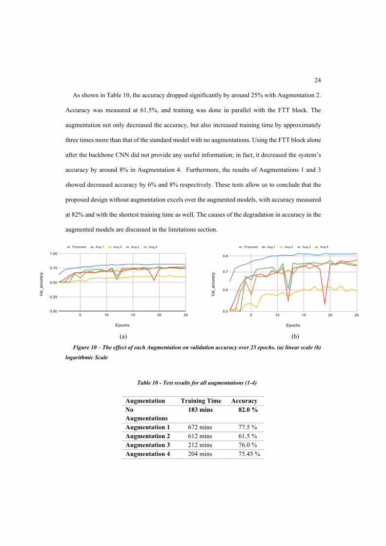
24

As shown in Table 10, the accuracy dropped significantly by around 25% with Augmentation 2.

Accuracy was measured at 61.5%, and training was done in parallel with the FTT block. The

augmentation not only decreased the accuracy, but also increased training time by approximately

three times more than that of the standard model with no augmentations. Using the FTT block alone

after the backbone CNN did not provide any useful information; in fact, it decreased the system’s

accuracy by around 8% in Augmentation 4. Furthermore, the results of Augmentations 1 and 3

showed decreased accuracy by 6% and 8% respectively. These tests allow us to conclude that the

proposed design without augmentation excels over the augmented models, with accuracy measured

at 82% and with the shortest training time as well. The causes of the degradation in accuracy in the

augmented models are discussed in the limitations section.

(a)

(b)

Figure 10 – The effect of each Augmentation on validation accuracy over 25 epochs. (a) linear scale (b)

logarithmic Scale

Table 10 - Test results for all augmentations (1-4)

Augmentation Training Time Accuracy

No

Augmentations

183 mins 82.0 %

Augmentation 1 672 mins 77.5 %

Augmentation 2 612 mins 61.5 %

Augmentation 3 212 mins 76.0 %

Augmentation 4 204 mins 75.45 %

25

6.4 Limitations and Future Work

Depth-wise separable convolution reduces the number of parameters while achieving the same

results as depth-wise convolution. It also produces new features after each convolution, combining

image channels to create new features, which depth-wise convolution does not do [40].

Extracting more features from the optical flow image can make the model under-fit the results,

because the extra details are not necessary and can be detrimental to the process. This can be

observed in both the augmentations and other CNN results. In the applied augmentation, MobileNet

[40] and the FTT [8] both utilize the depth-wise separable layers. Furthermore, Xception [22],

Inception [39] and the ResNet [21] family also rely on the same layer in their model. This explains

why the VGG [20] family had the highest accuracy when it was trained on images extracted from

optical flow information.

Another major limitation of this method is the fact that the sequence or the flow of the frames

must be preserved. Any false faces or unrelated images placed in the sequence will result in a false

optical flow image.

As seen in the results above, TPUs improve the time required to train and evaluate models. For

future work, training on TPUs with proper parameters and enough effort can lead to a huge

improvement in deepfake detection. As seen in the results, the training time is almost four times

faster than using the GPU. Also, in some instances like the ResNet, it actually performed better

than the GPU with the same input image size of 224x224. It will be necessary to explore more CNN

models in the future to find the advantages and limitations for this approach, similar to what was

done in examining the depth-wise separable layer.

7. Conclusions

In this research work, optical flow was used to detect deepfake videos by detecting

inconsistencies in video frames. The frames were cropped and transferred to a PWC-Net optical

flow estimator, which is a state-of-the-art tool created by NVIDIA. The resulting frames were then

26

sent to pre-trained image classification models such as VGG-16 and Xception in order to reuse the

training weights to cut down training time. These models were trained on GPU. The best performing

model was VGG-16, with 82.0% detection accuracy. Furthermore, the models were also trained on

TPUs. TPU training results proved that there is great potential for using this hardware in deepfake

detection and classification methods. The training time was cut by almost eight times for the same

model trained on a GPU. Also, some models actually improved detection accuracy compared to the

GPU results. In addition, four different augmentations were applied to the proposed method in order

to improve accuracy. However, detection accuracy was negatively affected by these augmentations.

Most of the tested models used depth-wise separator layers, which performed poorly in this method.

The top-performing model relied on the depth-wise convolution layer. The augmentations also used

depth-wise separator convolution layers, which affected the accuracy of the VGG-16 model

negatively. Researchers can use this work as the starting point in TPU utilization in detecting

deepfakes. Furthermore, it can be also used to explore the impact of augmentations on several

existing CNNs. As future work, training on TPUs with proper parameters can lead to a significant

improvement in deepfake detection. As the results showed, the time taken in training is almost four

times faster than using the GPU. Also, in some instances like the ResNet, it actually performed

better than the GPU with the same input image size of 224x224. Furthermore, it will be necessary

to explore more CNN models in the future to find the advantages and limitations for this approach,

similar to what was done in examining the depth-wise separable layer.

27

List of Abbreviations:

Graphics Processing Units (GPUs)

Tensor Processing Units (TPUs)

Convolutional Neural Network (CNN)

Artificial Intelligence (AI)

Photoplethysmography (PPG)

Recurrent neural network (RNN)

Generative Adversarial Networks (GANs)

Autoencoders (AEs)

Deepfake Detection Challenge dataset (DFDC)

Multiplier Accumulator (MAC)

Declarations

Availability of data and materials: The databases used in this research and their availability are

introduced in Section 3.2.

Compliance with Ethical Standards: The authors would like to convey their thanks and

appreciation to the “University of Sharjah” for supporting this work.

Conflict of Interest: The authors declare that they have no conflict of interest.

Informed consent: This study does not involve any experiments on animals.

Funding: This project is funded by Open UAE Research Group.

Acknowledgements: The authors would like to thank the Open UAE Research Group at UOS

Authors Information: ALI BOU NASSIF is currently the Assistant Dean of Graduate Studies at

the University of Sharjah, UAE. Ali is also an Associate Professor in the department of Computer

Engineering, as well as an Adjunct Research Professor at Western University, Canada. He obtained

28

a Master’s degree in Computer Science and a Ph.D. degree in Electrical and Computer Engineering

from Western University, Canada in 2009 and 2012, respectively. Ali’s research interests include the

applications of statistical and artificial intelligence models in different areas such as software

engineering, electrical engineering, e-learning, security, networking, signal processing and social

media. Ali has published more than 65 refereed conference and journal papers. Ali is a registered

professional engineer (P.Eng) in Ontario, as well as a member of IEEE Computer Society.

QASSIM NASIR is currently a professor of Electrical Engineering at the University of Sharjah and

the chairman of scientific publishing unit. Dr. Nasir current research interests are in

telecommunication and network security such as in CPS, IoT. He also conducts research in drone

and GPS jamming as well. He is a co-coordinator in OpenUAE research group which focuses on

blockchain performance and security, and the use of artificial intelligence in security applications.

Prior to joining the University of Sharjah, Dr. Nasir was working with Nortel Networks, Canada, as

a senior system designer in the network management group for OC-192 SONET. Dr. Nasir was

visiting professor at Helsinki University of Technology, Finland, during the summers of 2002 to

2009, and GIPSA lab, Grenoble France to work on a Joint research project on “MAC protocol and

MIMO” and “Sensor Networks and MIMO” research projects.

MANAR ABU TALIB is an associate professor at the University of Sharjah in the UAE. Dr. Abu

Talib’s research interest includes software engineering with substantial experience and knowledge

in conducting research in software measurement, software quality, software testing, ISO 27001 for

Information Security and Open-Source Software. Manar is also working on ISO standards for

measuring the functional size of software and has been involved in developing the Arabic version of

ISO 19761 (COSMIC-FFP measurement method). She published more than 50 refereed conferences,

journals, manuals and technical reports. She is the ArabWIC VP of Chapters in Arab Women in

Computing Association (ArabWIC), Google Women Tech Maker Lead, Co-coordinator of

OpenUAE Research & Development Group and the International Collaborator to Software

Engineering Research Laboratory in Montreal, Canada.

29

Omar Mohamed Gouda is a research assistant at the University of Sharjah, UAE. Omar is pursuing

his Master’s degree in Computer Engineering. Omar’s main interest of research includes

Optimization and the design and applications of Machine Learning and Deep Learning Applications

References

1. O. de Lima, S. Franklin, S. Basu, B. Karwoski, and A. George, ArXiv (2020).

2. T. Fagni, F. Falchi, M. Gambini, A. Martella, and M. Tesconi, ArXiv (2020).

3. R. Tolosana, R. Vera-Rodriguez, J. Fierrez, A. Morales, and J. Ortega-Garcia, DeepFakes and

Beyond: A Survey of Face Manipulation and Fake Detection (n.d.).

4. H. Khalid and S. S. Woo, in IEEE Comput. Soc. Conf. Comput. Vis. Pattern Recognit. Work.

(IEEE, 2020), pp. 2794–2803.

5. FaceApp, Faceapp (2018).

6. H. Qi, Q. Guo, F. Juefei-Xu, X. Xie, L. Ma, W. Feng, Y. Liu, and J. Zhao, in Proc. 28th ACM

Int. Conf. Multimed. (ACM, New York, NY, USA, 2020), pp. 4318–4327.

7. A. Rossler, D. Cozzolino, L. Verdoliva, C. Riess, J. Thies, and M. Niessner, in Proc. IEEE

Int. Conf. Comput. Vis. (2019), pp. 1–11.

8. H. Jeon, Y. Bang, and S. S. Woo, IFIP Adv. Inf. Commun. Technol. 580 IFIP, 416 (2020).

9. F. Matern, C. Riess, and M. Stamminger, in Proc. - 2019 IEEE Winter Conf. Appl. Comput.

Vis. Work. WACVW 2019 (2019), pp. 83–92.

10. Y. Li, X. Yang, P. Sun, H. Qi, and S. Lyu, in (Institute of Electrical and Electronics Engineers

(IEEE), 2020), pp. 3204–3213.

11. H. Gao, J. Pei, and H. Huang, in Proc. ACM SIGKDD Int. Conf. Knowl. Discov. Data Min.

(ACM, New York, NY, USA, 2019), pp. 1308–1316.

12. D. P. Kingma and P. Dhariwal, Adv. Neural Inf. Process. Syst. 2018-Decem, 10215 (2018).

13. J. Thies, M. Zollhöfer, M. Stamminger, C. Theobalt, and M. Nießner, in Commun. ACM

(2019), pp. 96–104.

14. G. Balakrishnan, F. Durand, and J. Guttag, in Proc. IEEE Comput. Soc. Conf. Comput. Vis.

Pattern Recognit. (2013), pp. 3430–3437.

15. B. Dolhansky, J. Bitton, B. Pflaum, J. Lu, R. Howes, M. Wang, and C. C. Ferrer, ArXiv

(2020).

16. D. Guera and E. J. Delp, in Proc. AVSS 2018 - 2018 15th IEEE Int. Conf. Adv. Video Signal-

30

Based Surveill. (2019), pp. 1–6.

17. I. Laptev, M. Marszałek, C. Schmid, and B. Rozenfeld, in 26th IEEE Conf. Comput. Vis.

Pattern Recognition, CVPR (2008).

18. I. Amerini, L. Galteri, R. Caldelli, and A. Del Bimbo, Deepfake Video Detection through

Optical Flow Based CNN (n.d.).

19. D. Sun, X. Yang, M. Y. Liu, and J. Kautz, IEEE Trans. Pattern Anal. Mach. Intell. 42, 1408

(2020).

20. E. Guerra, J. de Lara, A. Malizia, and P. Díaz, Inf. Softw. Technol. 51, 769 (2009).

21. K. He, X. Zhang, S. Ren, and J. Sun, in Proc. IEEE Comput. Soc. Conf. Comput. Vis. Pattern

Recognit. (IEEE Computer Society, 2016), pp. 770–778.

22. F. Chollet, in Proc. - 30th IEEE Conf. Comput. Vis. Pattern Recognition, CVPR 2017 (2017),

pp. 1800–1807.

23. T. Karras, T. Aila, S. Laine, and J. Lehtinen, in 6th Int. Conf. Learn. Represent. ICLR 2018

- Conf. Track Proc. (International Conference on Learning Representations, ICLR, 2018), pp. 1–

26.

24. L. Li, J. Bao, T. Zhang, H. Yang, D. Chen, F. Wen, and B. Guo, in Proc. IEEE Comput. Soc.

Conf. Comput. Vis. Pattern Recognit. (IEEE, 2020), pp. 5000–5009.

25. Y. Li, M. C. Chang, and S. Lyu, in 10th IEEE Int. Work. Inf. Forensics Secur. WIFS 2018

(2018), pp. 1–7.

26. G. Dai, J. Xie, and Y. Fang, in MM 2017 - Proc. 2017 ACM Multimed. Conf. (ACM Press,

New York, New York, USA, 2017), pp. 672–680.

27. S. Suwajanakorn, S. M. Seitz, and I. Kemelmacher-Shlizerman, Assoc. Comput. Mach.

Trans. Graph. 36, 1 (2017).

28. R. Prenger, R. Valle, and B. Catanzaro, in ICASSP, IEEE Int. Conf. Acoust. Speech Signal

Process. - Proc. (IEEE, 2019), pp. 3617–3621.

29. W. Zhao, Q. Xie, Y. Ma, Y. Liu, and S. Xiong, in 2020 IEEE Int. Conf. Image Process.

(IEEE, 2020), pp. 1561–1565.

30. S. Baker, S. Roth, D. Scharstein, M. J. Black, J. P. Lewis, and R. Szeliski, in Proc. IEEE Int.

Conf. Comput. Vis. (IEEE, 2007), pp. 1–8.

31. B. K. P. Horn and B. G. Schunck, Artif. Intell. 17, 185 (1981).

32. A. Dosovitskiy, P. Fischery, E. Ilg, P. Hausser, C. Hazirbas, V. Golkov, P. Van Der Smagt,

D. Cremers, and T. Brox, in Proc. IEEE Int. Conf. Comput. Vis. (IEEE, 2015), pp. 2758–2766.

33. K. Zhang, Z. Zhang, Z. Li, and Y. Qiao, IEEE Signal Process. Lett. 23, 1499 (2016).

31

34. L. Vinet and A. Zhedanov, J. Phys. A Math. Theor. 44, 085201 (2011).

35. N. Ketkar and N. Ketkar, in Deep Learn. with Python (Apress, Berkeley, CA, 2017), pp. 97–

111.

36. A. Krizhevsky, I. Sutskever, and G. E. Hinton, Commun. ACM 60, 84 (2017).

37. N. P. Jouppi, in Proc. - Int. Symp. Comput. Archit. (ACM, New York, NY, USA, 2017), pp.

1–12.

38. E. Ilg, N. Mayer, T. Saikia, M. Keuper, A. Dosovitskiy, and T. Brox, in Proc. - 30th IEEE

Conf. Comput. Vis. Pattern Recognition, CVPR 2017 (2017), pp. 1647–1655.

39. C. Szegedy, V. Vanhoucke, S. Ioffe, J. Shlens, and Z. Wojna, in Proc. IEEE Comput. Soc.

Conf. Comput. Vis. Pattern Recognit. (2016), pp. 2818–2826.

40. A. Howard, M. Sandler, B. Chen, W. Wang, L. C. Chen, M. Tan, G. Chu, V. Vasudevan, Y.

Zhu, R. Pang, Q. Le, and H. Adam, in Proc. IEEE Int. Conf. Comput. Vis. (IEEE, 2019), pp. 1314–

1324.