optical flow estimation - university of torontojepson/csc2503/opticalflow.pdf · optical flow...

Optical Flow Estimation

Goal: Introduction to image motion and 2D optical flow estimation.

Motivation:

• Motion is a rich source of information about the world:

– segmentation

– surface structure from parallax

– self-motion

– recognition

– understanding behavior

– understanding scene dynamics

• Other correspondence / registration problems:

– stereo disparity (short and wide baseline)

– computer-assisted surgery (esp. multi-modal registration)

– multiview alignment for mosaicing or stop-frame animation

Readings: Fleet and Weiss (2005)

Matlab Tutorials: intromotionTutorial.m, motionTutorial.m

2503: Optical Flow c©D.J. Fleet & A.D. Jepson, 2005 Page: 1

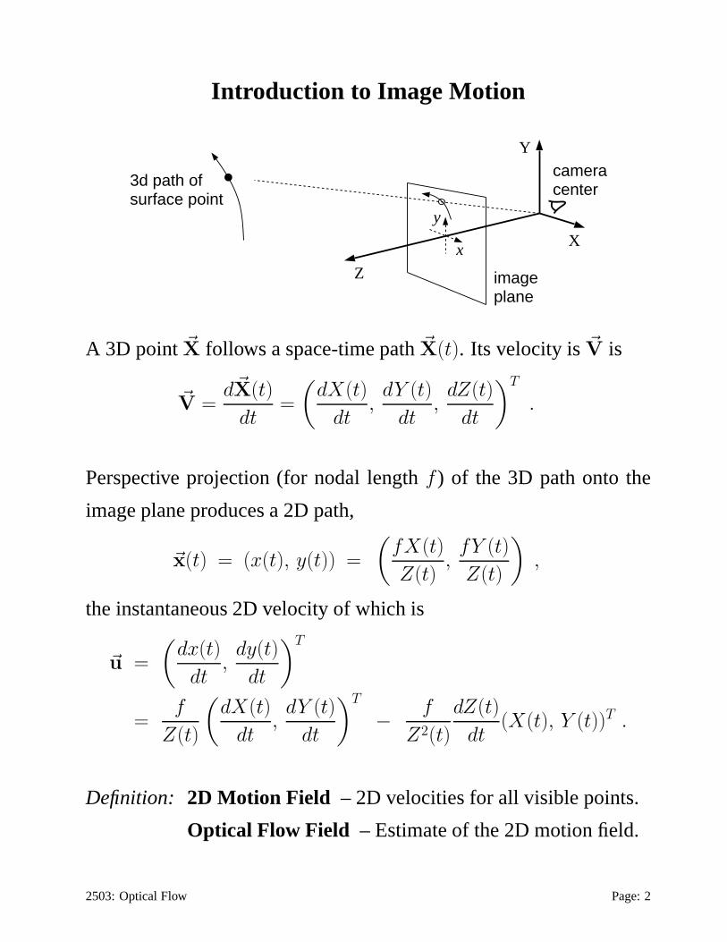
Introduction to Image Motion

cameracenter

imageplane

3d path ofsurface point

X

Y

Z

x

y

●

A 3D point ~X follows a space-time path~X(t). Its velocity is~V is

~V =d~X(t)

dt=

(

dX(t)

dt,

dY (t)

dt,

dZ(t)

dt

)T

.

Perspective projection (for nodal lengthf ) of the 3D path onto the

image plane produces a 2D path,

~x(t) = (x(t), y(t)) =

(

fX(t)

Z(t),

fY (t)

Z(t)

)

,

the instantaneous 2D velocity of which is

~u =

(

dx(t)

dt,

dy(t)

dt

)T

=f

Z(t)

(

dX(t)

dt,

dY (t)

dt

)T

− f

Z2(t)

dZ(t)

dt(X(t), Y (t))T .

Definition: 2D Motion Field – 2D velocities for all visible points.

Optical Flow Field – Estimate of the 2D motion field.

2503: Optical Flow Page: 2

Optical Flow

Two Key Problems:

1. Determine what image property to track.

2. Determine how to track it

Brightness constancy: Let’s track points of constant brightness,

assuming that surface radiance is constant over time:

I(x, y, t + 1) = I(x − u1, y − u2, t) .

Brightness constancy is often assumed by researchers, and often vi-

olated by Mother Nature; so the resulting optical flow field issome-

times a very poor approximation to the 2D motion field.

For example, a rotating Lambertian sphere with a static light source

produces a static image. But a stationary sphere with a moving light

source produces drifting intensities (figure from Jahne et al, 1999).


Gradient-Based Motion Estimation

How do we find the motion of a 1D greylevel functionf(x)? E.g.,

let’s say thatf(x) is displaced by distanced from time1 to time2:

f2(x) = f1(x − d) .

We can express the shifted signal as a Taylor expansion off1 aboutx:

f1(x − d) = f1(x) − d f ′1(x) + O(d2f ′′

1 ) ,

in which case the difference between the two signals is givenby

f2(x) − f1(x) = − d f ′1(x) + O(d2f ′′

1 ) .

Then, a first-order approximation to the displacement is

d =f1(x) − f2(x)

f ′1(x)

.

For linear signals the first-order estimate is exact.

For nonlinear signals, the accuracy of the approximation depends on

the displacement magnitude and the higher-order signal structure.


Gradient Constraint Equation

In two spatial dimensions we express the brightness constancy con-

straint as

f(x + u1 ,y + u2, t + 1) = f(x, y, t) (1)

As above, we substitute a first-order approximation,

f(x + u1 ,y + u2, t + 1) ≈f(x, y, t) + u1fx(x, y, t) + u2fy(x, y, t) + ft(x, y, t) (2)

into the left-hand side of (1), and thereby obtain thegradient con-

straint equation:

u1 fx(x, y, t) + u2 fy(x, y, t) + ft(x, y, t) = 0 .

Written in vector form, with~∇f ≡ (fx, fy)T :

~uT ~∇f(x, y, t) + ft(x, y, t) = 0 .

When the duration between frames is large, it is sometimes more ap-

propriate to use only spatial derivatives in the Taylor series approxi-

mation in (2). Then one obtains a different approximation

~uT ~∇f(x, y, t) + ∆f(x, y, t) = 0

where∆f(x, y, t) ≡ f(x, y, t + 1) − f(x, y, t).


Brightness Conservation

One can also derive the gradient constraint equation directly from brightness conservation.

Let (x(t), y(t)) denote a space-time path along which the image intensity remains is constant; i.e.,

the time-varying imagef satisfies

f(x(t), y(t), t) = c

Taking the total derivative of both sides gives

d

d tf(x(t), y(t), t) = 0

The total derivative is given in terms of its partial derivatives

d

d tf(x(t), y(t), t) =

∂f

∂x

dx

dt+

∂f

∂y

dy

dt+

∂f

∂t

dt

dt

= fx u1 + fy u2 + ft

= ~uT ~∇f + ft

= 0

This derivation assumes that there is no aliasing, so that one can in principle reconstruct the contin-

uous underlying signal and its derivatives in space and time. There are many situations in which this

is a reasonable assumption. But with common video cameras temporal aliasing is often a problem

with many video sequences, as we discuss later in these notes.

2503: Optical Flow Notes: 6

Normal Velocity

The gradient constraint provides one constraint in two unknowns. It

defines a line in velocity space:

l

motionconstraint

line

The gradient constrains the velocity in the direction normal to the

local image orientation, but does not constrain the tangential velocity.

That is, it uniquely determines only the normal velocity:

~un =−ft

||~∇f ||~∇f

||~∇f ||

When the gradient magnitude is zero, we get no constraint!

In any case, further constraints are required to estimate both elements

of the 2D velocity~u = (u1, u2)T .


Area-Based Regression

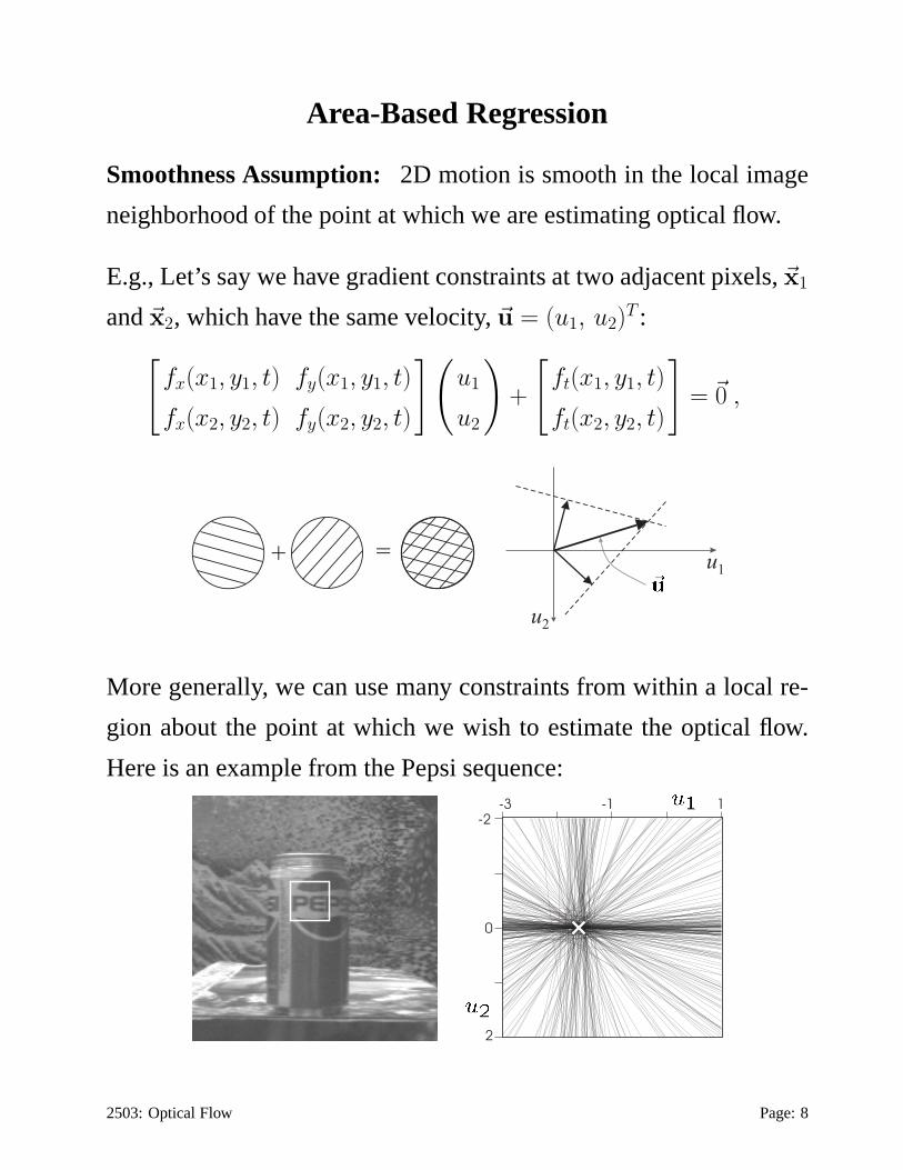
Smoothness Assumption: 2D motion is smooth in the local image

neighborhood of the point at which we are estimating opticalflow.

E.g., Let’s say we have gradient constraints at two adjacentpixels,~x1

and~x2, which have the same velocity,~u = (u1, u2)T :

[

fx(x1, y1, t) fy(x1, y1, t)

fx(x2, y2, t) fy(x2, y2, t)

](

u1

u2

)

+

[

ft(x1, y1, t)

ft(x2, y2, t)

]

= ~0 ,

u1

u2

+ =

More generally, we can use many constraints from within a local re-

gion about the point at which we wish to estimate the optical flow.

Here is an example from the Pepsi sequence:

-2

2

0

-1 1-3


Area-Based Regression (Linear LS)

We will not satisfy all constraints exactly. Rather we seek the velocity

that minimizes the squared error in each constraint (calledthe least-

squares (LS) velocity estimate):

E(u1, u2) =∑

x,y

g(x, y) [u1fx(x, y, t) + u2fy(x, y, t) + ft(x, y, t)]2

whereg(x, y) is a low-pass window that helps give more weight to

constraints at the center of the region.

Solution: DifferentiateE with respect to(u1, u2) and set to zero:

∂E(u1, u2)

∂u1=∑

xy

g(x, y)[

u1 fx2 + u2 fx fy + fx ft

]

= 0

∂E(u1, u2)

∂u2=∑

xy

g(x, y)[

u2 fy2 + u1 fx fy + fy ft

]

= 0

The constraints thus yield two linear equations foru1 andu2.

In matrix notation, thesenormal equationsand their solution are

M ~u + ~b = ~0 , u = −M−1~b

(assumingM−1 exists), where

M =∑

g

(

fx

fy

)

(fx, fy) =

[

∑

g fx2 ∑

g fxfy∑

g fxfy

∑

g fy2

]

~b =∑

g ft

(

fx

fy

)

=

(

∑

g fxft∑

g fyft

)


Area-Based Regression (Implementation)

Since we want the optical flow at each pixel, we can compute thecomponents of the normal equa-

tions with a set of image operators. This is much prefered to looping over image pixels.

1. First, compute 3 image gradient images at time t, corresponding to the gradient measurements:

fx(~x) , fy(~x) , ft(~x)

2. Point-wise, we compute the quadratic functions of the derivative images. This produces five

images equal to:

f 2

x(~x) , f 2

y (~x) , fx(~x)fy(~x) , ft(~x)fy(~x) , ft(~x)fx(~x)

3. Blurring the quadratic images corresponds to the accumulating of local constraints under the

spatial (or spatiotemporal) support windowg above. This produces five images, each of which

contains an element of the normal equations at a specific image locations:

g(~x) ∗ f 2

x(~x) , g(~x) ∗ f 2

y (~x) ,

g(~x) ∗ [fx(~x) fy(~x)] , g(~x) ∗ [ft(~x) fy(~x)] , g(~x) ∗ [ft(~x) fx(~x)]

4. Compute the two images containing the components of optical flow at each pixel. This is

given in closed form since the inverse of the normal matrix (i.e.,M above) is easily expressed

in closed form.


Aperture Problem

Even with the collection of constraints from within a region, the esti-

mation will be undetermined when the matrixM is singular:

u1

u1

u2

u2

When all image gradients are parallel, then the normal matrix for the

least-squares solution becomes singular (rank 1). E.g., for gradients

m(x, y)~n, wherem(x, y) is the gradient magnitude at pixel(x, y)

M =

(

∑

x,y

g(x, y) m2(x, y)

)

~n ~nT

Aperture Problem: For sufficiently small spatial apertures the nor-

mal matrix,M, will be singular (rank deficient).

Generalized Aperture Problem: For small aperturesM becomes

singular, but for sufficiently large apertures the 2D motionfield may

deviate significantly from the assumed motion model.

Heuristic Diagnostics: Use singular values,s1≥s2 ≥s3, of∑

x,y g ~h ~hT,

for ~h = (fx, fy, ft)T , to assess the rank of the local image structure:

– if s2 is ”too small” then only normal velocity is available

– if s3 is ”large” then the gradient constraints do not lie in a plane

so a single velocity will not fit the data well.

Such ”bounds” will depend on the LS region size and the noise.


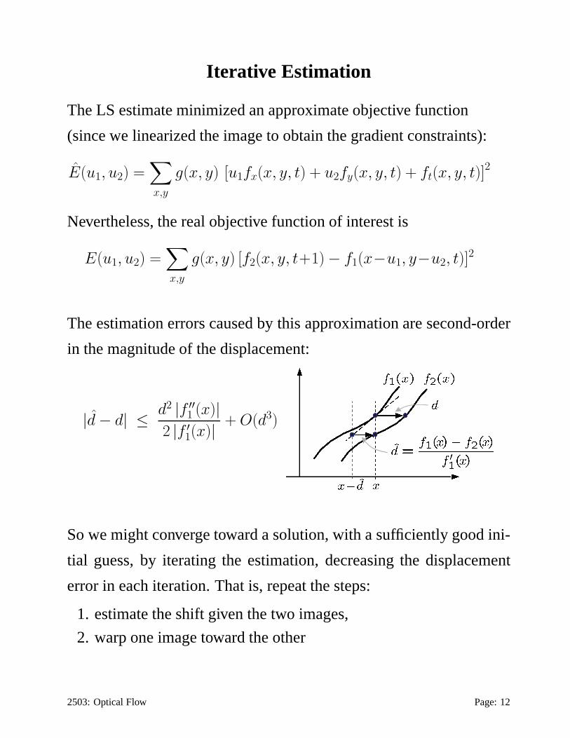
Iterative Estimation

The LS estimate minimized an approximate objective function

(since we linearized the image to obtain the gradient constraints):

E(u1, u2) =∑

x,y

g(x, y) [u1fx(x, y, t) + u2fy(x, y, t) + ft(x, y, t)]2

Nevertheless, the real objective function of interest is

E(u1, u2) =∑

x,y

g(x, y) [f2(x, y, t+1) − f1(x−u1, y−u2, t)]2

The estimation errors caused by this approximation are second-order

in the magnitude of the displacement:

|d − d| ≤ d2 |f ′′1 (x)|

2 |f ′1(x)| + O(d3)

So we might converge toward a solution, with a sufficiently good ini-

tial guess, by iterating the estimation, decreasing the displacement

error in each iteration. That is, repeat the steps:

1. estimate the shift given the two images,

2. warp one image toward the other


Iterative Estimation (cont)

xx0

Initial guess:

Estimate:

Initial guess:

Estimate:

estimateupdate

xx0xx0xx0

Initial guess:

Estimate:

Initial guess:

Estimate:

estimateupdate

xx0xx0xx0

Initial guess:

Estimate:

Initial guess:

Estimate:

Initial guess:

Estimate:

Initial guess:

Estimate:

Initial guess:

Estimate:

estimateupdate


Image Warps

Example:3 iterations of refinement (from the motion tutorial). Here,

vSandv denote the preshift velocity and the LS estimate. Figure axes

represent incremental horizontal and vertical velocities(givenvS).

Some practical issues:

• initially, if the displacement is large, many of the constraints

might be very noisy

• warping introduces interpolation noise, so stick to integer warps

if possible.

• warp one image, take derivatives of the other so you don’t need

to re-compute the gradient after each iteration.

• often useful to low-pass filter the images before motion estima-

tion (for better derivative estimation, and somewhat better linear

approximations to image intensity)2503: Optical Flow Page: 14

Aliasing

When a displacement between two frames is too large (i.e., when a

sinusoid is displaced a half a wavelength or more), the inputis aliased.

This is caused by fast shutter speeds in most cameras.

no aliasing aliasing

Aliasing often results in convergence to the wrong 2D optical flow.

Possible Solutions:

1. prediction from previous estimates topre-warpthe next image

2. use feature correspondence to establish rough initial match

3. coarse-to-fine estimation: Progressive flow estimation from

coarse to fine levels within Gaussian pyramids of the two images.

• start at coarsest level,k = L , warp images with initial guess,

then iterate warping & LS estimation until convergence to~uL.

• warp levelsk = L − 1 using −~uL, then apply iterative esti-

mation until convergence~uL−1.

...

• warp levelsk = 0 (i.e., the original images) using~u1, then

apply iterative estimation until convergence.


Higher-Order Motion Models

Constant flow model within an image neighborhood is often a poor

model, especially when the regions become larger. Affine models

often provide a more suitable model of local image deformation.

Translation Scaling Rotation ShearTranslation Scaling Rotation Shear

Affine flow for an image region centered at location~x0 is given by

~u(~x) =

(

a1 a2

a3 a4

)

(~x − ~x0) +

(

a5

a6

)

= A(~x;~x0)~a

where~a = (a1, a2, · · · , a6)T and

A(~x;~x0) =

[

x−x0 y−y0 0 0 1 0

0 0 x−x0 y−y0 0 1

]

Then the gradient constraint becomes:

0 = ~u(x, y)T ~∇f(x, y, t) + ft(x, y, t)

= ~aTA(x, y)T ~∇f(x, y, t) + ft(x, y, t) ,

so, as above, the weighted least-squares solution for~a is given by:

a = M−1~b

where, for weighting with the spatial windowg,

M =∑

x,y

g(~x)AT ~∇f ~∇fTA , ~b = −

∑

x,y

g(~x)AT ~∇f ft


Similarity Transforms

There are many classes of useful motion models. Simple translation and affine deformations are the

commonly used motion models.

Another common motion model is a special case of affine deformation called a similarity deforma-

tion. It comprises a uniform scale change, along with a rotation and translation:

~u(~x) = α

(

cos θ − sin θ

sin θ cos θ

)

(~x − ~x0) +

(

d1

d2

)

We can also express this transform as a linear function of a somewhat different set of motion model

parameters. In particular, in matrix form we can write a similarity transform as

~u(x, y) = A(x, y)~a

where~a = (α cos θ, α sin θ, d1, d2)T , and

A =

(

x − x0 −y + y0 1 0

y − y0 x − x0 0 1

)

With this form of the similarity transform, we can formulatea LS estimator for similarity transforms

in the same way we did for the affine motion model.

There are other classes of motion model that are also very important. One such class is the 2D

homography (we’ll discuss this later).


Robust Motion Estimation

Sources of heavy-tailed noise (outliers): specularities &highlights,

jpeg artifacts, interlacing, motion blur, large displacements, and mul-

tiple motions (occlusion boundaries, transparency, etc.)

Problem: Least-squares estimators are extremely sensitive to outliers

error penalty function influence functionerror penalty function influence functionerror penalty function influence function

Solution: Redescending error functions (e.g., Geman-McClure) help

to reduce influence of outliers:

error penalty function influence functionerror penalty function influence function

Previous objective function:

E(~u) =∑

x,y

g(~x) [f(~x, t+1) − f(~x−~u, t)]2

Robust objective function:

E(~u) =∑

x,y

g(~x) ρ(f(~x, t+1) − f(~x−~u, t))


Probabilistic Motion Estimation

Probabilistic formulations allow us to address issues of noisy mea-

surements, confidence measures, and prior beliefs about themotion.

Formulation: Measurements of image derivatives, especiallyft, are

noisy. Let’s assume that spatial derivatives are accurate,but temporal

derivative measurements have additive Gaussian noise:

ft(x, y, t) = ft(x, y, t) + η(x, y, t)

whereη(x, y, t) has a mean-zero Gaussian density with varianceσ2.

Then, given the gradient constraint equation, it follows that

~uT ~∇f + ft ∼ N(0, σ2)

So, if we know~u, then the probability of observing(~∇f, ft) is

p(~∇f, ft | ~u) =1√2πσ

exp

(

−(~uT ~∇f + ft)2

2σ2

)

Assuming constraints atN pixels, each with IID Gaussian noise, the

joint likelihood is the product of the individual likelihoods:

L(~u) =∏

x,y

p(~∇f(~x, t), ft(~x, t) | ~u)


Optimal Estimation

Maximum likelihood (ML): Find the flow~u that maximizes the

probability of observing the data given~u. Often we instead minimize

the negative log likelihood:

L(~u) = −∑

x,y

log p(~∇f(~x, t), ft(~x, t) | ~u)

= −N log(√

2πσ) +∑

x,y

(~u(~x, t) · ~∇f(~x, t) + ft(~x, t))2

2σ2

Note: L is identical to our previous objective functionE except for

the supportg(x, y) and the constant term.

Maximum A Posteriori (MAP): Include prior beliefs,p(~u), and use

Bayes’ rule to express the posterior flow distribution:

p(~u | {~∇f, ft}~x) =p({~∇f, ft}~x | ~u) p(~u)

p({~∇f, ft}~x)

For example, assume a (Gaussian) slow motion prior:

p(~u) =1√2πσ

exp

(−~uT~u

2σ2u

)

Then the flow that maximies the posterior is given by

u =

(

M +1

σ2u

I

)−1

~b

where

M =1

σ2

∑

x,y

~∇f ~∇fT , ~b = − 1

σ2

∑

x,y

~∇f ft


ML / MAP Estimation (cont)

Remarks:

• The inverse Hessian of the negative log likelihood providesa

measure of estimator covariance (easy for Gaussian densities).

• Alternative noise models can be incorporated in spatial andtem-

poral derivatives (e.g., total least squares). One can alsoassume

non-Gaussian noise and outliers (to obtain robust estimators)

• Other properties of probabilistic formulation: Ability topropa-

gate ”distributions” to capture belief uncertainty.

• Use of probabilistic calculus for fusing information from other

sources


Layered Motion Models

Layered Motion:

The scene is modeled as a cardboard cutout. Each layer has an as-

sociated appearance, an alpha map (specifying opacity or occupancy

in the simplest case), and a motion model. Layers are warped by the

motion model, texture-mapped with the appearance model, and then

combined according to their depth-order using the alpha maps.


Further Readings

M. J. Black and P. Anandan. The robust estimation of multiplemotions: Parametric and piecewise-

smooth flow fields.Computer Vision and Image Understanding, 63:75–104, 1996.

J. L. Barron, D. J. Fleet, and S. S. Beauchemin. Performance of optical flow techniques.Interna-

tional Journal of Computer Vision, 12(1):43–77, 1994.

J. R. Bergen, P. Anandan, K. Hanna, and R. Hingorani. Hierarchical model-based motion estima-

tion. Proc. Second European Conf. on Comp. Vis., pp. 237–252. Springer-Verlag, 1992.

D. J. Fleet and Y. Weiss. Optical flow estimation. InMathematical models for Computer Vision:

The Handbook. N. Paragios, Y. Chen, and O. Faugeras (eds.), Springer, 2005.

A. Jepson and M. J. Black. Mixture models for optical flow computation. Proc. IEEE Conf.

Computer Vision and Pattern Recognition, pp. 760–761, New York, June 1993.

E P Simoncelli, E H Adelson, and D J Heeger. Probability distributions of optical flow. Proc.

Conf. Computer Vision and Pattern Recognition, pp. 310–315, Mauii, HI, June 1991.

J.Y.A. Wang and E.H. Adelson. Representing moving images with layers,IEEE Trans. on Image

Processing,3(5):625–638, 1994.

Y. Weiss and E.H. Adelson. A unified mixture framework for motion segmentation: Incorporating

spatial coherence and estimating the number of models.IEEE Proc. Computer Vision and

Pattern Recognition,San Francisco, pp. 321–326, 1996.


optical flow estimation - university of torontojepson/csc2503/opticalflow.pdf · optical flow...

Documents