lcmrl: improved estimation of quantitation limits · lcmrl: improved estimation of quantitation...

A World of Solutions

LCMRL: Improved Estimation of Quantitation Limits

@ Pittcon 2015

John H Carson Jr., PhD CB&I Federal Services LLC

Robert O’Brien

Steve Winslow CB&I Federal Services LLC

Steve Wendelken USEPA, OGWDW

David Munch USEPA, OGWDW (retired)


1

LCMRL stands for Lowest Concentration Minimum Reporting Limit

– Reporting Limit based on a defined accuracy of measurement objective

– Measurement Quality Objective (MQO)

– EPA is only organization using this term and concept

– Lowest true sample concentration such that individual measurements meet a specified MQO with high probability

Statistical estimate of the LCMRL

What is the LCMRL?


2

Currie (1968) – Applied stat decision theory to detection limits (LC, LD)

– Determination Limit (LQ) -- S/N = 10

Hubaux & Vos (1970) – Applied regression analysis to Currie’s approach

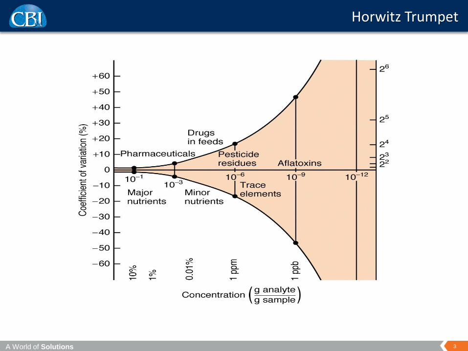
Horwitz et al. (1980) – Power law for std dev of repeated measurement

Glaser et al. (1981) – EPA Lab in Cincinnati developed MDL, practical procedure for

determining Currie’s LC and LQ

Rocke and Lorenzato (1995) – Analytical error is combination of additive and multiplicative errors

– Error variance does not 0 as concentration 0

Summary of some prior developments


3

Horwitz Trumpet


4

MQO: the measured concentration is within 50% of true concentration (50-150% recovery)

LCMRL is lowest concentration that meets the MQO criterion with 99% probability

To use both precision and bias in the analysis

– non-constant error variance

– imperfect calibration

– possible nonlinearity of response

To make estimates robust against outliers in data

To develop a robust algorithm and computational code that can handle “bad data” without crashing

To develop an LCMRL calculator for end users

USEPA OGWDW Objectives


5

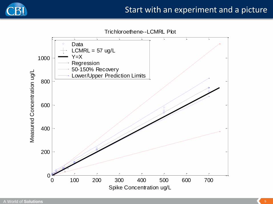
Start with an experiment and a picture

0 100 200 300 400 500 600 7000

200

400

600

800

1000

Trichloroethene--LCMRL Plot

Spike Concentration ug/L

Mea

sure

d C

once

ntr

ati

on

ug/L

Data LCMRL = 57 ug/L Y=X Regression 50-150% Recovery Lower/Upper Prediction Limits


6

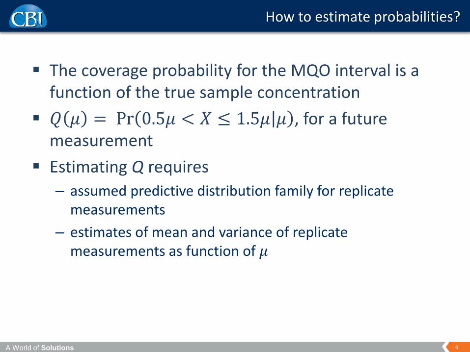
The coverage probability for the MQO interval is a function of the true sample concentration

𝑄 𝜇 = Pr 0.5𝜇 < 𝑋 ≤ 1.5𝜇 𝜇 , for a future measurement

Estimating Q requires

– assumed predictive distribution family for replicate measurements

– estimates of mean and variance of replicate measurements as function of 𝜇

How to estimate probabilities?


7

Estimation of conditional mean response function is a regression problem

– measured regressed onto “true”

– Also estimates conditional bias

Estimation of conditional replicate variance function is also a regression problem

Choice of measurement distribution family

– Prefer maximum entropy distributions with specified mean and variance of response distribution

– Normal when measurements can be negative

– Gamma, when measurements cannot be negative

Conditional Distribution of Response


8

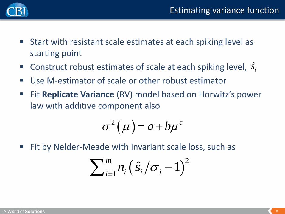
Start with resistant scale estimates at each spiking level as starting point

Construct robust estimates of scale at each spiking level,

Use M-estimator of scale or other robust estimator

Fit Replicate Variance (RV) model based on Horwitz’s power law with additive component also

Fit by Nelder-Meade with invariant scale loss, such as

Estimating variance function

2 ca b

2

1ˆ 1

m

i i iin s

is


11

Non-constant variance + possible outliers use Iteratively Reweighted Least Squares (IRLS)

Weights are product of

– robust weights to minimize impact of ‘outliers’ and

– reciprocal of variance function

Possible nonlinearity at upper end use low order polynomial

Estimating mean response function


12

Methods often designed to operate in linear range, BUT

Typical calibration experiments for analytical instruments – Usually do not include replication

– Usually have 5 or fewer design points

– Often will not detect nonlinearity in response function

Typical LCMRL experiment has – 4 replicates

– 7 or 8 design points in low working range

LCMRL experiment allows estimation of bias, including nonlinearity, not otherwise detectable

Why nonlinearity?


13

Nonlinearity at low concentration caused by non-ideal processes in measurement such as: – Presence of analyte interferent

– Analyte absorption or degradation by instrument

– Loss of analyte in extraction step

– Matrix enhancement

Polynomial only handles loss of linearity at high end

Mean-squared error (MSE) function – Incorporates error due to nonlinearity at low end of curve

– Modeled using constant + power function

– Estimation similar to variance function

– Captures part of lack of fit (Type III error)

Mean squared error function


14

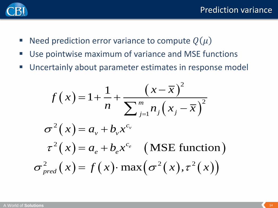
Need prediction error variance to compute 𝑄 𝜇

Use pointwise maximum of variance and MSE functions

Uncertainly about parameter estimates in response model

Prediction variance

2

2

1

2

2

2 2 2

11

MSE function

max ,

v

e

m

j jj

c

v v

c

e e

pred

x xf x

n n x x

x a b x

x a b x

x f x x x


15

Distributional family + mean response curve + prediction variance curve completely define an estimated distribution of replicate measurements at each true sample concentration.

Can directly estimate as function of sample concentration probability that sample recovery is between 50% and 150%.

At this point finding LCMRL is a numerical optimization problem.

EPA LCMRL Calculator software makes LCMRL usable for labs.

Calculator download and technical manual are at http://water.epa.gov/scitech/drinkingwater/labcert/analyticalmethods_ogwdw.cfm#four

Predictive distribution

http://water.epa.gov/scitech/drinkingwater/labcert/analyticalmethods_ogwdw.cfm#four




16

0 0.05 0.1 0.15 0.2 0.250

0.05

0.1

0.15

0.2

0.25

0.3

0.35

0.4

1,4-dioxane--LCMRL Plot


Mea

sure

d C

once

ntra

tion

ug/L

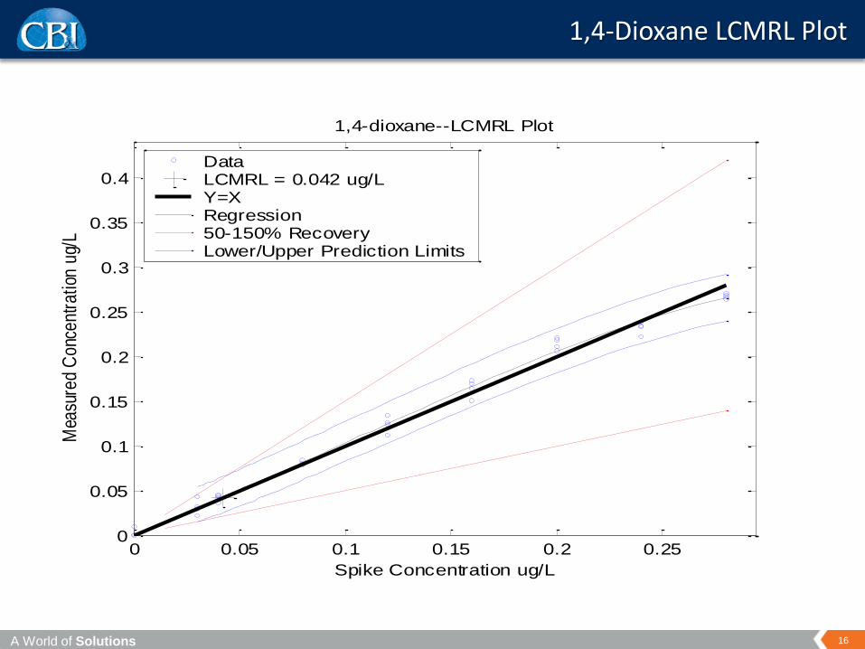
Data LCMRL = 0.042 ug/L Y=X Regression 50-150% Recovery Lower/Upper Prediction Limits

1,4-Dioxane LCMRL Plot


17

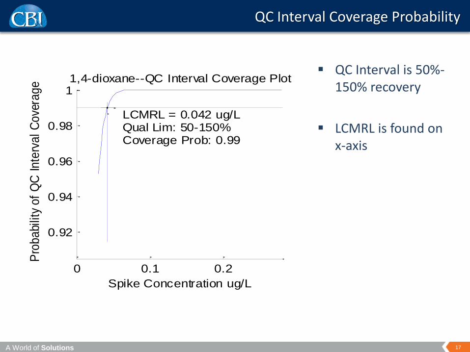
QC Interval is 50%-150% recovery

LCMRL is found on x-axis

QC Interval Coverage Probability

0 0.1 0.2

0.92

0.94

0.96

0.98

1

LCMRL = 0.042 ug/L Qual Lim: 50-150% Coverage Prob: 0.99

1,4-dioxane--QC Interval Coverage Plot


Pro

ba

bilit

y o

f Q

C I

nte

rva

l C

ove

rag

e


18

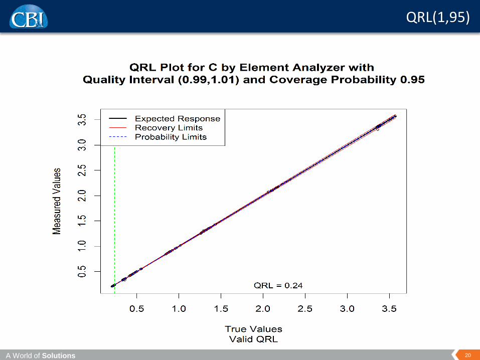
Quality Reporting Limit (QRL) defined as lowest true sample value such that measured result expected to be within 100 ± Q% of true value C% of the time—QRL(Q,C)

LCMRL is QRL(50,99)

In some cases, response is mass rather than concentration

Not always possible to have replicates at exactly the same values

– Compositional analysis

– Need a lot more data in this case, but it is doable

QRL – Generalization of LCMRL


19

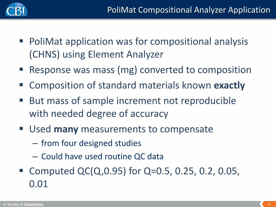
PoliMat application was for compositional analysis (CHNS) using Element Analyzer

Response was mass (mg) converted to composition

Composition of standard materials known exactly

But mass of sample increment not reproducible with needed degree of accuracy

Used many measurements to compensate

– from four designed studies

– Could have used routine QC data

Computed QC(Q,0.95) for Q=0.5, 0.25, 0.2, 0.05, 0.01

PoliMat Compositional Analyzer Application


20

QRL(1,95)


21

0.5 1.0 1.5 2.0 2.5 3.0 3.5

0.5

1.5

2.5

3.5

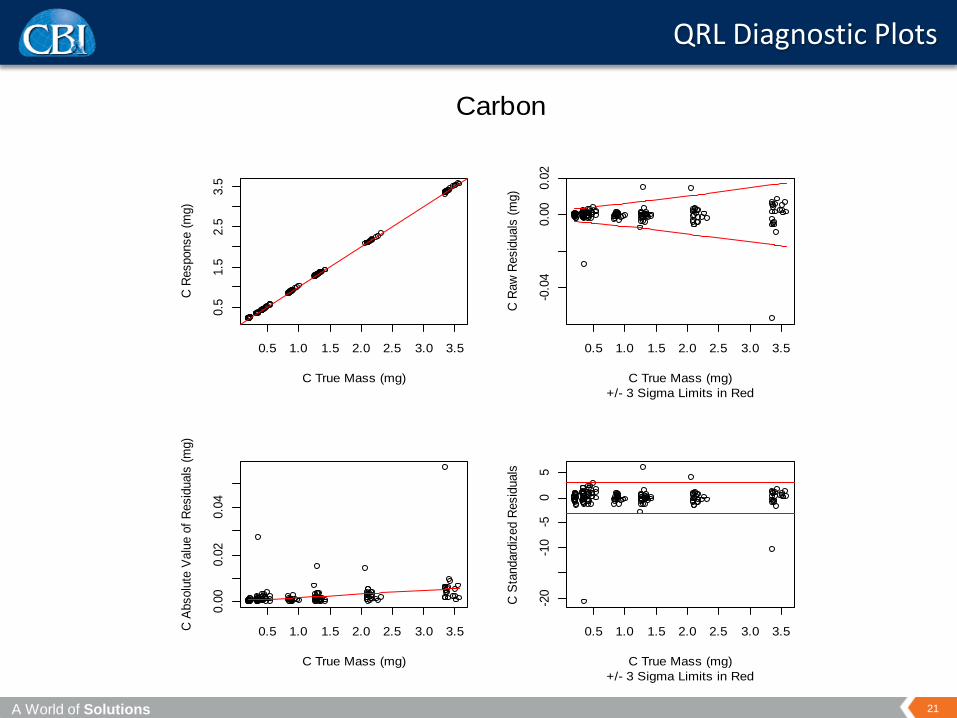
C True Mass (mg)

C R

esponse (

mg)

0.5 1.0 1.5 2.0 2.5 3.0 3.5

-0.0

40.0

00.0

2

+/- 3 Sigma Limits in Red

C True Mass (mg)

C R

aw

Resid

uals

(m

g)

0.5 1.0 1.5 2.0 2.5 3.0 3.5

0.0

00.0

20.0

4

C True Mass (mg)

C A

bsolu

te V

alu

e o

f R

esid

uals

(m

g)

0.5 1.0 1.5 2.0 2.5 3.0 3.5

-20

-10

-50

5

+/- 3 Sigma Limits in Red

C True Mass (mg)

C S

tandard

ized R

esid

uals

Carbon

QRL Diagnostic Plots


22

Affiliated and supporting procedures:

– MRL, essentially a programmatic LCMRL upper limit, is already done

– LCMRL/MRL quick validation procedure

– Revamping lab QC program to monitor LCMRL at similar cost

– Extending to other matrices through standard additions

Fully Bayesian implementation via MCMC

Multianalyte LCMRL method, requires Bayesian MCMC implementation

Development as ASTM standard practice

What Next?


23

This work has been funded by USEPA under contract (EP-C-06-031) to Shaw Environmental, Inc (now CBI Federal Services LLC) and under contract (EP-C-07-022) to The Cadmus Group, Inc.

EPA OGWDW Program Managers—Steve Wendelken, David Munch (retired)

CBI statisticians—John Carson, Robert O’Brien

CBI principal analyst—Steve Winslow, extensive testing, feedback and supplying test data sets

CBI project manager—Mike Zimmerman

Acknowledgements


24

Questions?

John H. Carson, Jr PhD

Senior Statistician

CB&I Federal Services LLC

+1 419-429-5519

[email protected]

Questions


25

Contact

For further information, contact

John H. Carson, Jr PhD

Senior Statistician

CB&I Federal Services LLC

+1 419-429-5519

[email protected]


26

Currie, L. A. (1968), “Limits for Qualitative Detection and Quantitative Determination.” Analytical Chemistry, Vol. 40, pp. 586-593.

Horwitz W, Kamps LR, Boyer KW. (1980) Quality assurance in the analysis of foods and trace constituents. Journal of the Association of Official Analytical Chemists. 63(6):1344-54.

Glaser, J. A., Foerst, D. L., McKee, G. D., Quane, S. A. and W. L. Budde (1981), “Trace Analyses for Wastewaters.” Environmental Science and Technology. Vol. 15, pp. 1426-1435.

Hubaux, Andre and Gilbert Vos (1970), “Decision and Detection Limits for Linear Calibration Curves.” Analytical Chemistry. Vol. 42, No. 8, pp. 849-855.

Rocke, D.M. and S. Lorenzato (1995), “A Two-Component Model for Measurement Error in Analytical Chemistry.” Technometrics. Vol. 37, No. 2, pp. 176-184.

Analytical Chemistry References


27

Horn, Paul S. (1988) “A Biweight Prediction Interval for Random Samples.” Journal of the American Statistical Association. Vol. 83, No. 401. (Mar., 1988), pp. 249-256.

Kagan, A. M.; Linnik, Yu. V. and C. R. Rao (1973) Characterization Problems in Mathematical Statistics. John Wiley. New York. 499 pp.

Lax, D. A. (1985), “Robust estimators of scale: Finite-sample performance in long-tailed symmetric distributions,” Journal of the American Statistical Association. Vol. 80, pp. 736-741.

Nelder, J.A. and R. Mead (1965), “A Simplex Method for Function Minimization”, Computer Journal. Vol. 7, pp. 308-313.

Rousseeuw, P.J. and C. Croux (1993) “Alternatives to the Median Absolute Deviation” Journal of the American Statistical Association. Vol. 88, No. 424 (Dec., 1993), pp. 1273-1283.

Statistical References

lcmrl: improved estimation of quantitation limits · lcmrl: improved estimation of quantitation...

Documents