improved large-step markov chain variants for the
TRANSCRIPT

Journal of Heuristics, 3, 63–81 (1997)c© 1997 Kluwer Academic Publishers. Manufactured in The Netherlands.
Improved Large-Step Markov Chain Variants forthe Symmetric TSP
INKI HONG, ANDREW B. KAHNG {inki, abk}@cs.ucla.eduUCLA Computer Science Department Los Angeles, CA 90095-1596 USA
BYUNG-RO MOON [email protected] Technology Research Center, LG Semicon Co., Ltd. 16 Woomyon-dong, Seocho-gu, Seoul, Korea
Abstract. Thelarge-step Markov chain(LSMC) approach is the most effective known heuristic for large symmetricTSP instances; cf. recent results of [Martin, Otto and Felten, 1991] and [Johnson, 1990]. In this paper, we examinerelationships among (i) the underlying local optimization engine within the LSMC approach, (ii) the “kick move”perturbation that is applied between successive local search descents, and (iii) the resulting LSMC solution quality.We find that the traditional “double-bridge” kick move is not necessarily optimum: stronger local optimizationengines (e.g., Lin-Kernighan) are best matched with stronger kick moves. We also propose use of an adaptivetemperature schedule to allow escape from deep basins of attraction; the resultinghierarchical LSMC variantoutperforms traditional LSMC implementations that use uniformly zero temperatures. Finally, a population-basedLSMC variant is studied, wherein multiple solution paths can interact to achieve improved solution quality.
Keywords: Large-step Markov chain, optimization, simulated annealing, traveling salesman problem
1. Preliminaries
Given a set of cities and a symmetric matrix of all inter-city distances, the symmetrictraveling salesman problem (TSP) seeks a shortest tour which visits each city exactly once.The symmetric TSP is NP-hard [Garey and Johnson, 1979], and has been extensively studiedboth in terms of its combinatorial structure and as a testbed for exact and heuristic methods[Lawler et al., 1985] [Johnson and McGeoch, 1997]. Studies such as [Johnson, 1990] pointto greedy local search (e.g., using the fast 3-Opt [Bentley, 1992] or the Lin-Kernighan(LK) [Lin and Kernighan, 1973] neighborhood structure) as the most effective approachfor practical instances. Over the past decade,iterated descent[Baum, 1986a] [Baum,1986b] has been shown to be an effective means of applying a given greedy local search“engine”: iteratively perform a greedy descent, then perturb the resulting local minimum toobtain the starting solution for the next greedy descent. Currently, the “large-step Markovchain” (LSMC) heuristic of [Martin, Otto and Felten, 1991] and the “iterated LK” heuristicof [Johnson, 1990] are believed to be the best-performing iterated descent variants (and,indeed, the best-performing of all heuristics for obtaining near-optimal solutions [Johnsonand McGeoch, 1997]); we generically refer to both of these as LSMC methods.

64 HONG, KAHNG AND MOON
1.1. Previous Large-Step Markov Chain Implementations
Table 1.The LSMC algorithm
Algorithm LSMC
Input: TSP instance, iteration boundM , temperature scheduletempi, i = 1, . . . ,MOutput: heuristic tourTbest
1. Generate a random tourTinit;
2. T1 = Descent(Tinit);
3. Tbest = T1;
4. for i = 1 to M
(A) Ti∗ = kick move(Ti);
(B) Ti∗∗ = Descent(Ti∗);
(C) diff = cost(Ti∗∗) − cost(Ti);(D) if ( diff < 0 ), then Ti+1 = Ti
∗∗;else{
i. generate a random numbert ∈ [0, 1);
ii. if ( t < exp(− diff /tempi ) ), then Ti+1 = Ti∗∗, elseTi+1 = Ti;
}(E) if ( cost(Tbest) >cost(Ti∗∗) ) Tbest = Ti
∗∗;
5. return Tbest;
The LSMC approach is described in Table 1, following the presentation in [Martin, Ottoand Felten, 1991]. LSMC alternately applies (i) a (greedy) local optimization procedureDescent, followed by (ii) a “kick move” which perturbs the current local minimum solutionin order to obtain a starting solution for the nextDescentapplication. Local search (i.e.,De-scent) procedures used in previous implementations include LK as well ask-Opt methods.1
[Martin, Otto and Felten, 1991] used both LK and a fast implementation of 3-Opt; [John-son, 1990] used LK only. Kick move perturbation of the current local minimum tour istypically achieved using ak′-change, withk′ not necessarily equal tok. Both [Martin, Ottoand Felten, 1991] and [Johnson, 1990] use random “double-bridge” 4-change kick moves,illustrated in Figure 1. According to [Martin, Otto and Felten, 1991], the double-bridgekick move is chosen for its ability to produce large-scale changes in the current tour withoutdestroying the solution quality via too large a random perturbation. Furthermore, it is arelatively small perturbation whose “non-sequential” structure [Lin and Kernighan, 1973]is not easily reproduced by the Lin-Kernighan algorithm.
As can be seen from Table 1, the LSMC method actually performs simulated annealingover local minima, with{ kick move +Descent } as the neighborhood operator. In otherwords, if a new local minimum has lower cost than its predecessor, it is always adoptedas the current solution; otherwise, it is adopted with probability given by the Boltzmann


66 HONG, KAHNG AND MOON
1.2. Scope of the Present Study
In this work, we study the performance of LSMC on randomly-generated symmetric TSPinstances4 using a variety of local optimization heuristics and kick moves. In particular,we examine relationships among (i) the underlying local optimization engine within theLSMC approach, (ii) the “kick move” perturbation that is applied between successive localsearch descents, and (iii) the resulting LSMC solution quality. In Section 2, we showthat the traditional “double-bridge” kick move is not necessarily optimum: stronger localoptimization engines (e.g., Lin-Kernighan) are best matched with stronger kick moves.In Section 3, we also propose use of a simple adaptive temperature schedule to allowescape from deep basins of attraction; the resultinghierarchicalLSMC variant outperformstraditional LSMC implementations that use uniformly zero temperatures. Finally, Section4 studies a population-based LSMC variant wherein multiple solution paths are allowed tocooperate in order to possibly achieve improved solution quality.
Our experiments use 2-Opt, 3-Opt and LK local optimization engines provided by [Boese,1995]. These codes implement speedups of 2- and 3-Opt which are described in [Bent-ley, 1992] and reviewed in [Johnson and McGeoch, 1997]. Using a strategy originallydue to Lin and Kernighan [Lin and Kernighan, 1973], aneighbor-liststores the 25 nearestneighbors for each city; this is implemented via thek-d tree [Bentley, 1990] data structureand simplifies finding improving moves or verifying local optimality. Following the termi-nology of [Johnson, 1990] [Baum, 1986a] [Baum, 1986b], we call the associated LSMCimplementations Iterated 2-Opt, Iterated 3-Opt and Iterated LK, respectively.
As testbeds, we use three instances whose optimal tour costs are known. LIN318 andATT532 are well-known geometric TSP instances used in many other studies, e.g., [Martin,Otto and Felten, 1991] [Martin, Otto and Felten, 1992] [Martin and Otto, 1996] [Johnson,1990]; the former has 318 city locations and is due to Lin and Kernighan [Lin and Kernighan,1973], while the latter is derived from the locations of 532 cities in the continental UnitedStates. The optimal tour lengths are known to be 42029 (LIN318) and 27686 (ATT532).5
The third instance is S800, an 800-city random symmetric instance with integer inter-citydistances randomly chosen from the interval[1, 10000]. The optimal tour length for S800is known to be 20328 [Applegate et al., 1995].
Generally, all performance comparisons in this paper are based on the averages of solutioncosts over 50 trials.6 The average running times are reported in CPU seconds on an HP-Apollo 9000/735 workstation.
2. Studies of Kick Move Strength
The studies of [Baum, 1986a] [Baum, 1986b] and [Martin, Otto and Felten, 1991] clearlypoint out the effect of kick move choice on solution quality. Intuitively, the kick move sizeshould be such that (i) it is likely that the search can reach a new basin of attraction, yet(ii) the current level of solution quality is not lost through random perturbation. As notedabove, both [Martin, Otto and Felten, 1991] and [Johnson, 1990] used the double-bridge4-change kick move. [Martin, Otto and Felten, 1991] allowed only kick moves that did


68 HONG, KAHNG AND MOON
kick moves. For the random symmetric instance (S800), 3-change always seems to producethe best results. This evidence suggests that the traditional double-bridge 4-change kickmove is suboptimal, particularly for the geometric instances that are so frequently studiedin the literature.
3. Adaptive Temperature Schedules
Recall that LSMC may be viewed as a variant of simulated annealing that moves amonglocal optima, and that the annealing temperature in previous LSMC studies was typicallyset to zero (or left unspecified if non-zero temperatures were used). Also recall that thesuccess of zero-temperature LSMC has led [Martin and Otto, 1996] [Applegate et al., 1995]to explicitly conjecture or implicitly assume that the LSMC cost surface (under the{ kickmove +Descent } neighborhood operator) has very few local minima. However, it is ourexperience that zero-temperature LSMC is often trapped in local minima which are notglobally optimum. Thus, in this section we propose use of stronger perturbations whichenable escape from spurious local minima. This results in ahierarchical LSMCapproach,with non-zero annealing temperatures constituting a “higher-level kick move” that is appliedwhen the LSMC search is perceived to be trapped. Baum [Baum, 1986a] [Baum, 1986b] alsoraised the issue of escaping spurious local minima, and proposed applying a (structurally)stronger kick move while remaining within the zero-temperature regime.
In our simple variant of hierarchical LSMC, the original zero-temperature LSMC isconsidered “stuck” if no local minimum has been accepted in the last2n iterations (forIterated 2-Opt and Iterated 3-Opt) or in the last 100 iterations (for Iterated LK). Whenthe zero-temperature LSMC becomes stuck, the annealing temperature is set to the currentsolution costcost(Ti) divided by 200, for 100 iterations, after which it is reset to zero.10
Table 2 compares the performance of our hierarchical LSMC implementation with that ofzero-temperature LSMC for Iterated 2-Opt, Iterated 3-Opt and Iterated LK. We report datafor both the 4-change kick move and the most successful kick move among those testedin Section 2.11 For the two geometric instances, hierarchical LSMC clearly outperformszero-temperature LSMC. The advantage of hierarchical LSMC is less obvious for the S800instance, except when used with the Iterated LK engine. Generally, for S800 we findthat zero-temperature LSMC is only rarely “stuck”; understanding this phenomenon is aninteresting future direction.
4. Population-Based Search
LSMC executes a “monolithic” or “single-threaded” search, i.e., only one solution is savedat any given time. It is intriguing to consider the contrast between the single-threaded LSMCsearch and, e.g., “adaptive multi-start” techniques [Boese, Kahng and Muddu, 1994] whichexploit structural relationships among local optima [Boese, 1995].12 Taking advantage ofrelationships between high quality solutions is also a feature of tabu search intensifica-tion strategies, which employ strongly determined and consistent variables together withmemory-based processes to reinforce or reinstate attributes of elite solutions (see, e.g.,

IMPROVED LARGE-STEP MARKOV 69
Table 2.Performance of hierarchical LSMC (t 6= 0) versus zero-temperature LSMC (t = 0). (a) Iterated 2-Opt(b) Iterated 3-Opt (c) Iterated LK
(a)
Instance LIN318 ATT532 S800
Number of 4-change 5-change 4-change 7-change 4-change 3-changeIterations t = 0 t 6= 0 t = 0 t 6= 0 t = 0 t 6= 0 t = 0 t 6= 0 t = 0 t 6= 0 t = 0 t 6= 0
1000 .872 .840 .822 .805 .699 .689 .688 .670 77.3 77.3 77.8 77.82000 .658 .524 .596 .535 .528 .512 .486 .453 66.3 66.3 65.4 65.43000 .548 .469 .463 .413 .475 .458 .416 .386 59.6 59.6 58.9 58.94000 .458 .356 .410 .324 .432 .412 .354 .342 55.4 55.4 54.6 54.65000 .405 .309 .381 .308 .401 .375 .335 .311 51.9 51.9 51.4 51.46000 .384 .362 .312 .298 49.3 49.3 48.9 48.97000 .371 .349 .300 .288 47.0 47.0 46.9 46.98000 .353 .321 .278 .267 44.9 44.9 45.2 45.29000 .342 .289 .262 .251 43.3 43.3 43.7 43.710000 .330 .262 .250 .239 41.7 41.7 42.2 42.2
(b)
Instance LIN318 ATT532 S800
Number of 4-change 8-change 4-change 8-change 4-change 3-changeIterations t = 0 t 6= 0 t = 0 t 6= 0 t = 0 t 6= 0 t = 0 t 6= 0 t = 0 t 6= 0 t = 0 t 6= 0
1000 .175 .143 .107 .095 .142 .142 .136 .136 12.83 12.83 13.19 13.192000 .147 .059 .091 .037 .106 .097 .101 .103 11.46 11.46 11.37 11.373000 .129 .037 .065 .007 .099 .082 .087 .091 10.55 10.55 10.37 10.374000 .124 .019 .054 .006 .093 .073 .082 .080 9.93 9.93 9.65 9.655000 .105 .000 .047 .000 .088 .064 .080 .072 9.36 9.36 9.18 9.186000 .081 .062 .069 .064 9.01 9.01 8.81 8.817000 .079 .060 .064 .059 8.73 8.73 8.45 8.458000 .076 .059 .062 .048 8.42 8.42 8.17 8.179000 .075 .057 .060 .046 8.17 8.17 7.91 7.9110000 .075 .056 .060 .044 7.95 7.95 7.70 7.70
(c)
Instance LIN318 ATT532 S800
Number of 4-change 8-change 4-change 15-change 4-change 3-changeIterations t = 0 t 6= 0 t = 0 t 6= 0 t = 0 t 6= 0 t = 0 t 6= 0 t = 0 t 6= 0 t = 0 t 6= 0
200 .153 .151 .093 .089 .125 .125 .129 .129 1.641 1.641 1.796 1.796400 .082 .048 .020 .017 .095 .093 .091 .090 1.589 1.590 1.471 1.471600 .047 .017 .012 .007 .078 .076 .071 .070 1.368 1.411 1.378 1.378800 .012 .005 .003 .002 .068 .065 .064 .063 1.281 1.282 1.378 1.3761000 .005 .000 .000 .000 .063 .060 .060 .058 1.250 1.282 1.378 1.1691200 .061 .057 .051 .046 1.250 1.275 1.173 1.1691400 .058 .053 .050 .043 1.250 1.272 1.095 1.0951600 .056 .051 .042 .037 1.250 1.258 1.095 1.0921800 .052 .048 .038 .033 1.218 1.258 1.095 1.0882000 .050 .045 .033 .031 1.218 1.257 1.067 1.059
[Glover, 1977], [Glover and Laguna, 1993]). In this section, we note thatpopulation-basedsearchoffers a convenient framework for hybridizing monolithic search and multi-startsearch. Within this framework, we ask whether solution quality can be improved by usinga population of local search processes which have “evolutionary” interdependencies. Forexample, some fixed number of solutions may be evolved according to evolutionary pro-gramming [Fogel, Owens and Walsh, 1966] or “go with the winners” [Aldous and Vazirani,1994] paradigms, each of which uses an evolving population with no concept of “crossover”.
Given a fixed CPU budget ofM descents, a population sizep, and an “update interval”I, our population-based LSMCapproach follows the outline of Table 3: we maintain apopulation ofp separate LSMC searches that interact everyp · I descents. More precisely,we initially computep local minima and then repeat the following main loop untilMdescents have been performed. In the loop,I zero-temperature{ kick move +Descent} cycles are applied to each of thep existing solutions. Then, one solution (Tj) is chosen

70 HONG, KAHNG AND MOON
Table 3.A template for population-based LSMC
Algorithm: Population-based (zero-temperature) LSMC
Input: TSP instance, iteration boundM , population sizep, update intervalIOutput: heuristic tourTbest
1. For i = 1 to p,
(A) generate a random tourTi;
(B) Ti =Descent(Ti);
Tbest = minimum-cost tour among allTi’s;
2. do {
(A) For each solutionTi, do the followingI times:
i. Ti∗ = kick move(Ti);
ii. Ti∗∗ = Descent(Ti∗);
iii. if ( cost(Ti∗∗ < cost(Ti) ) Ti = Ti∗∗;
iv. if ( cost(Tbest) > cost(Ti∗∗) ) Tbest = Ti
∗∗;
(B) Choose a solutionTj based on proportional selection;
(C) Tj∗ = kick move(Tj);
(D) Tj∗∗ = Descent(Tj∗);
(E) if ( cost(Tbest) > cost(Tj∗∗) ) Tbest = Tj
∗∗;
(F) ReplaceTj∗∗ with a solution in the population;
} while ( number ofDescents performed is≤M );
3. return Tbest;
based on a roulette-wheel selection scheme [Goldberg, 1989] wherein the best solution isfour times as likely to be selected as the worst solution. If one more{ kick move +Descent} cycle applied toTj produces a new solutionTj
∗∗ that is better thanTj , thenTj∗∗ replaces
Tj in the current population. Otherwise,Tj∗∗ replaces the worst solution in the current
population, as long asTj∗∗ has better cost than this solution.
A wide spectrum of population-based LSMC implementations is possible, based on thevalue ofI. At one extreme,I = 0 and thep solution streams have the strongest possibleinteraction: no iterations are made before the next solution is selected for possible replace-ment. At the other extreme,I =∞ is equivalent to multi-start LSMC withp independentruns ofM/p descents each. In our tests, we tried 3-Opt and LK as the local optimizationengine with the double-bridge 4-change kick move; examining all possible combinationswas beyond the scope of our study. Values ofI = 0, 5, 10, 20 and∞ were tested withpopulation sizesp = 5, 10 and 20. A fixed CPU budget was used for all experiments; forIterated 3-Opt (Iterated LK), we usedM = 5000 (M = 1000) descents for LIN318 andM = 10000 (M = 2000) descents for ATT532. Tables 4, 5 and 6 show that for Iterated

IMPROVED LARGE-STEP MARKOV 71
Table 4.Population-based LSMC with 3-Opt descent engine: Relationship between update interval and solutioncost for population size 5. (a) LIN318 (b) ATT532
(a)
Iter. I = 0 I = 5 I = 10 I = 20 Independent
1000 .129 .038 .066 .050 .0672000 .105 .014 .021 .023 .0213000 .077 .011 .016 .014 .0104000 .076 .011 .016 .009 .0055000 .068 .011 .016 .005 .004
(b)
Iter. I = 0 I = 5 I = 10 I = 20 Independent
1000 .128 .144 .148 .138 .1512000 .105 .101 .099 .099 .1043000 .093 .091 .091 .087 .0884000 .088 .083 .083 .076 .0815000 .082 .081 .080 .072 .0776000 .073 .077 .076 .070 .0727000 .071 .076 .073 .065 .0678000 .071 .070 .072 .060 .0649000 .067 .070 .066 .056 .06110000 .066 .068 .066 .055 .060
Table 5.Population-based LSMC with 3-Opt descent engine: Relationship between update interval and solutioncost for population size 10. (a) LIN318 (b) ATT532
(a)
Iter. I = 0 I = 5 I = 10 I = 20 Independent
1000 .063 .079 .077 .064 .0822000 .053 .031 .019 .012 .0273000 .049 .018 .005 .002 .0084000 .041 .010 .004 .001 .0035000 .037 .001 .004 .000 .003
(b)
Iter. I = 0 I = 5 I = 10 I = 20 Independent
1000 .141 .195 .186 .203 .2042000 .108 .116 .102 .126 .1253000 .094 .088 .088 .098 .0914000 .085 .078 .071 .084 .0765000 .082 .072 .068 .074 .0706000 .077 .065 .063 .069 .0637000 .074 .061 .060 .067 .0618000 .074 .060 .059 .063 .0579000 .073 .059 .054 .060 .05510000 .069 .057 .054 .057 .052

72 HONG, KAHNG AND MOON
Table 6.Population-based LSMC with 3-Opt descent engine: Relationship between update interval and solutioncost for population size 20. (a) LIN318 (b) ATT532
(a)
Iter. I = 0 I = 5 I = 10 I = 20 Independent
1000 .049 .100 .117 .128 .1252000 .016 .039 .035 .043 .0373000 .011 .015 .020 .018 .0134000 .011 .004 .004 .009 .0055000 .011 .001 .002 .004 .002
(b)
Iter. I = 0 I = 5 I = 10 I = 20 Independent
1000 .169 .260 .264 .264 .2692000 .121 .153 .166 .161 .1743000 .100 .116 .123 .121 .1234000 .087 .086 .106 .097 .1045000 .083 .072 .086 .081 .0916000 .080 .063 .080 .073 .0817000 .078 .060 .073 .069 .0728000 .072 .058 .069 .064 .0659000 .072 .053 .065 .057 .06110000 .069 .049 .061 .054 .057
Table 7. Population-based LSMC with LK descent engine: Relationship between update interval and solutioncost for population size 5.(a) LIN318 (b) ATT532
(a)
Iter. I = 0 I = 5 I = 10 I = 20 Independent
200 .089 .120 .078 .077 .093400 .039 .049 .027 .013 .035600 .020 .034 .013 .011 .014800 .000 .014 .006 .000 .0111000 .000 .000 .000 .000 .000
(b)
Iter. I = 0 I = 5 I = 10 I = 20 Independent
200 .105 .174 .159 .177 .161400 .077 .111 .095 .123 .099600 .064 .082 .075 .090 .079800 .060 .068 .070 .073 .0681000 .057 .061 .062 .058 .0611200 .056 .057 .058 .051 .0601400 .052 .051 .048 .047 .0541600 .048 .046 .043 .046 .0521800 .048 .044 .040 .043 .0512000 .048 .043 .037 .040 .049
IMPROVED LARGE-STEP MARKOV 73
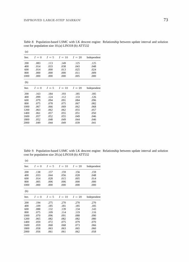
Table 8. Population-based LSMC with LK descent engine: Relationship between update interval and solutioncost for population size 10.(a) LIN318 (b) ATT532
(a)
Iter. I = 0 I = 5 I = 10 I = 20 Independent
200 .083 .113 .149 .125 .125400 .014 .033 .038 .043 .048600 .014 .000 .013 .025 .024800 .000 .000 .000 .011 .0091000 .000 .000 .000 .005 .000
(b)
Iter. I = 0 I = 5 I = 10 I = 20 Independent
200 .163 .184 .193 .185 .185400 .099 .124 .112 .133 .126600 .079 .094 .091 .084 .096800 .075 .078 .075 .067 .0821000 .067 .066 .069 .062 .0681200 .063 .062 .062 .055 .0571400 .061 .057 .055 .051 .0501600 .057 .052 .055 .049 .0461800 .052 .048 .049 .044 .0462000 .049 .044 .049 .039 .041
Table 9. Population-based LSMC with LK descent engine: Relationship between update interval and solutioncost for population size 20.(a) LIN318 (b) ATT532
(a)
Iter. I = 0 I = 5 I = 10 I = 20 Independent
200 .138 .157 .159 .156 .159400 .033 .044 .056 .028 .048600 .014 .028 .015 .005 .014800 .005 .006 .006 .000 .0001000 .000 .000 .000 .000 .000
(b)
Iter. I = 0 I = 5 I = 10 I = 20 Independent
200 .194 .275 .270 .270 .270400 .109 .185 .181 .185 .185600 .088 .132 .139 .134 .143800 .075 .109 .114 .119 .1161000 .070 .096 .091 .088 .0901200 .065 .082 .082 .082 .0801400 .059 .072 .075 .079 .0701600 .059 .068 .068 .073 .0661800 .058 .063 .063 .065 .0602000 .056 .061 .061 .062 .058

74 HONG, KAHNG AND MOON
3-Opt, the combination (I = 20, p = 10) was best for LIN318, while the combination(I = 5, p = 20) was best for ATT532. Tables 7, 8 and 9 show that for Iterated LK, thecombination (I = 5, p = 10) was best for LIN318, while the combination (I = 10, p = 5)was best for ATT532. Note that the original Iterated 3-Opt (Iterated LK) studied in Section 2averages.105% (.005%) above optimum for LIN318 and.075% (.050%) above optimumfor ATT532, while the best population-based LSMC variant with 3-Opt (LK) local opti-mization engine averages0% (0%) above optimum for LIN318 and.049% (.037%) aboveoptimum for ATT532.
In our population-based LSMC approach, the parameterI trades off between coupling ofthep search processes and diversity among thep current solutions. Our experimental dataindicate that even pure multi-start LSMC (I = ∞) is superior to the original LSMC. Atthe same time, it seems obvious that for very small CPU budgets, lower values ofI (e.g.,I = 0) will be the most successful. Tuning the values ofp andI to a given instance andCPU budgetM remains an open issue.
5. Conclusion
We have provided extensive experimental studies of traditional zero-temperature LSMC,following the original implementations reported by [Martin, Otto and Felten, 1991] and[Johnson, 1990]. Experiments with variousk-change kick moves suggest that the traditionaldouble-bridge 4-change kick move is not optimum, and that the best kick move stronglydepends on both the underlying local optimization engine and the type of instance.13 Wehave also proposed ahierarchical LSMCstrategy which significantly improves performanceover the previous zero-temperature LSMC implementations. Further studies might addressin more detail the relationship between optimal temperature schedules and structural pa-rameters of the cost surface. Finally, we have proposed the use ofpopulation-based LSMCstrategies which again seem to offer improvements over the previous LSMC implemen-tations. Here, the key open issue involves tuning the update interval and population sizeparameters to the given problem instance and CPU budget.
Acknowledgments
We thank Kenneth D. Boese for providing source codes for the local optimization enginesused in this study. We also thank David S. Johnson and Kenneth D. Boese for their valuablecomments and careful reading of this manuscript.
Notes
1. Some fairly standard terminology: Ak-change operation modifies the current tour by removing up tokexisting edges and reconnecting the resulting tour fragments into a new tour. Ak-Opt method uses greedysearch within thek-change neighborhood structure. A tour is “k-Opt” if it is locally minimum with respect tothek-change neighborhood structure.

IMPROVED LARGE-STEP MARKOV 75
2. In [Martin, Otto and Felten, 1991], the use of non-zero temperature was discussed in the context of the LIN318example, but no details of the implementation were given.
3. Martin and Otto [Martin and Otto, 1996] have recently conjectured that for instances of “moderate” size (e.g.,the ATT532 instance from TSPLIB) zero-temperature LSMC can be expected to return the global minimumsolution, since the LSMC cost surface has at most only a few local minima. That zero-temperature LSMChas very few basins of attraction is also in some sense an implicit assumption of Applegate et al. [Applegateet al., 1995], who use the union of edges in a very small number (10) of LSMC solutions to generate a goodbounding solution within a branch-and-bound approach; this method has resulted in several recent “world’srecords” for optimal solution of large TSP instances.
4. Our instances have distance matrices either (i) corresponding to randomly-generated pointsets in the Euclideanplane, or (ii) corresponding to independent random inter-city distances taken from a uniform distribution.
5. City locations are specified by integer coordinates in the Euclidean plane. Inter-city distances are maintainedas double-precision reals, and tour costs are rounded to the nearest integer.
6. The exception is the Iterated LK results for instance S800; running times were such that we are able to reportonly the average of 2 trials.
7. Efforts to contact the authors of [Martin, Otto and Felten, 1991] in order to determine the value of this “smallinteger” have been unsuccessful.
8. In other words, there may be many ways to reconnect the tour fragments in, say, a 7-change – but we alwaysreconnect the fragments in the same way. There were two exceptions to this practice: for 3-change werandomly chose among the four possible patterns that could reconnect the tour fragments, and for 4-changewe used the (unrestricted) double-bridge 4-change as in [Johnson, 1990].
9. Johnson and McGeoch [Johnson and McGeoch, 1997] usesn Iterated LK iterations for ann-city TSP instance.Thus, our tables also include data forn/8, n/4, n/2 andn iterations of Iterated LK, as well as data forn/2andn iterations of the other two methods.
10. Hence, the probability of acceptance isexp(−200 · diff/cost(Ti)), e.g., acceptance probability1/e for an0.5% cost increase. We also tried two other hierarchical LSMC variants. In the first, the temperature is raisedto cost(Ti)/100 and linearly cooled back to zero over 100 iterations; in the second, the temperature is raisedto +∞ for a small number of iterations (both 3 and 5 were tested) and then reset to zero. Results for thesevariants were essentially identical to the results that we report here.
11. Due to the definition of the “stuck” criterion, there is no difference between the zero-temperature and hier-archical LSMC implementations forn or fewer iterations; thus, we do not report results for small iterationbounds.
12. LSMC might be viewed as constituting search along the “boundary” of the “big valley” that governs 2-Opt, 3-Opt and LK local minima [Boese, Kahng and Muddu, 1994] [Boese, 1995]. Adaptive multi-starttechniques attempt to restart the local search in the “interior” of this big valley. Cf. hybrid genetic-local searchmetaheuristics, e.g., [M¨uhlenbein, Georges-Schleuter and Kr¨amer, 1988] [Ulder et al., 1990].
13. Recall that we used a fixed “template” to implement thek-change kick move for most values ofk studied.It is possible that otherk-change templates, or the use of randomk-changes, would yield different results.At present, we cannot assess the “strength” of ak-change kick move as a function ofk; it would be usefulto develop a quantitative measure which enables more precise study of the relationship between perturbationstrength and LSMC performance.
References
Aldous, D. and U. Vazirani, “‘Go with the winners’ algorithms,”Proc. IEEE Symp. on Foundations of ComputerScience, pages 492-501, 1994.
Applegate, D. L., July 1995, Personal Communication.Applegate, D. L., R. Bixby, V. Chvatal and W. Cook, “Finding cuts in the TSP (a preliminary report),” Technical
Report No. 95-05, Center for Discrete Mathematics and Theoretical Computer Science, 1995.Baum, E. B., “Iterated descent: A better algorithm for local search in combinatorial optimization problems,”
Manuscript, 1986a.Baum, E. B., “Towards practical ‘neural’ computation for combinatorial optimization problems,”Neural Networks
for Computing, AIP Conference Proceedings, page 151, 1986b.

76 HONG, KAHNG AND MOON
Bentley, J. L., “K-d trees for semidynamic point sets,”Proc. ACM Symp. on Computational Geometry, pages187–197, June 1990.
Bentley, J. L., “Fast algorithms for geometric traveling salesman problems,”ORSA Journal on Computing,4(4):387-411, 1992.
Boese, K. D., “Cost versus distance in the traveling salesman problem,” Technical Report TR-950018, UCLA CSDepartment, 1995.
Boese, K. D., A. B. Kahng, and S. Muddu, “A new adaptive multi-start technique for combinatorial globaloptimizations,”Operations Research Letters, 16(2):101-113, 1994.
Fogel, L. J., A. J. Owens, and M. J. Walsh,Artificial Intelligence Through Simulated Evolution, John Wiley, 1966.Garey, M. R. and D. S. Johnson,Computers and Intractability: A Guide to the Theory of NP-Completeness, W.
H. Freeman, New York, 1979.Glover, F., “Heuristics for integer programming using surrogate constraints,”Decision Sciences, 8:156-166, 1977.Glover, F., “Tabu search and adaptive memory programming – advances, applications and challenges,” In R. Barr,
R. Helgason, and J. Kennington, editors,Interfaces in Computer Science and Operations Research, pages 1-75,Kluwer Academic Publishers, 1996.
Glover, F. and M. Laguna, “Tabu search,” In C. Reeves, editor,Modern Heuristic Techniques for CombinatorialProblems, pages 70-141. Blackwell Scientific Publishing, Oxford, 1993.
Goldberg, D. E.,Genetic Algorithms in Search, Optimization and Machine Learning, Addison-Wesley, Reading,MA, 1989.
Johnson, D. S., “Local optimization and the traveling salesman problem,”Proc. 17th Intl. Colloquium onAutomata, Languages and Programming, pages 446-460, 1990.
Johnson, D. S. and L. A. McGeoch, “The traveling salesman problem: A case study in local optimization,” InE. H. L. Aarts and J. K. Lenstra, editors,Local Search Algorithms. Wiley and Sons, New York, 1997.
Lawler, E. L., J. K. Lenstra, A. Rinnooy-Kan, and D. Shmoys,The Traveling Salesman Problem: A Guided Tourof Combinatorial Optimization, Wiley, Chichester, 1985.
Lin, S. and B. W. Kernighan, “An effective heuristics algorithm for the traveling-salesman problem,”OperationsResearch, 31:498-516, 1973.
Martin, O. and S. W. Otto, “Combining simulated annealing with local search heuristics,” In G. Laporte, I. H.Osman, and P. L. Hammer, editors,Annals of Operations Research, volume 63, pages 57-75. 1996.
Martin, O., S. W. Otto, and E. W. Felten, “Large-step markov chains for the traveling salesman problem,”ComplexSystems, 5(3):299-326, June 1991.
Martin, O., S. W. Otto, and E. W. Felten, “Large-step markov chains for the TSP incorporating local searchheuristics,”Operations Research Letters, 11(4):219-224, 1992.
Muhlenbein, H., M. Georges-Schleuter, and O. Kr¨amer, “Evolution algorithms in combinatorial optimization,”Parallel Computing, 7:65-85, 1988.
Ulder, N. L. J., E. H. L. Aarts, H.-J. Bandelt, P. J. M. van Laarhoven, and E. Pesch, “Genetic local search algorithmsfor the traveling salesman problem,”Proc. Parallel Problem Solving from Nature, pages 109-116, 1990.

IMPROVED LARGE-STEP MARKOV 77
Appendix
Table A.1.Relationship between kick-move strength and performance of Iterated 2-Opt for LIN318.t - CPU seconds. MS - Multi-Start
MS 2-change 3-change 4-change 5-change 6-change 7-changeIter Cost t Cost t Cost t Cost t Cost t Cost t Cost t
159 3.47 14 6.4 0 2.02 1 1.96 1 1.86 2 2.02 2 2.03 2318 3.17 28 6.4 1 1.47 2 1.44 3 1.38 3 1.52 4 1.48 41000 2.90 91 6.4 2 .937 6 .872 9 .822 10 .923 12 .831 122000 2.70 182 6.4 4 .706 12 .658 18 .596 20 .682 24 .604 243000 2.65 274 6.4 6 .641 18 .548 27 .463 30 .596 36 .549 354000 2.59 365 6.4 8 .597 24 .458 35 .410 40 .540 48 .512 485000 2.51 456 6.4 10 .588 30 .405 44 .381 50 .487 60 .481 60
8-change 9-change 10-change 12-change 15-change 20-change 50-changeIter Cost t Cost t Cost t Cost t Cost t Cost t Cost t
159 2.16 2 2.20 2 2.26 3 2.01 3 1.89 3 1.98 4 2.10 4318 1.69 4 1.71 5 1.81 5 1.49 5 1.45 6 1.48 6 1.81 81000 .999 14 1.10 15 1.09 16 .875 17 .921 19 .987 21 1.27 252000 .759 28 .783 30 .769 31 .664 34 .700 38 .830 42 1.04 503000 .631 42 .605 45 .637 47 .604 51 .610 57 .741 62 .931 754000 .548 56 .501 59 .561 62 .569 68 .565 76 .682 83 .863 1005000 .483 69 .449 74 .517 78 .535 85 .538 94 .624 103 .819 125
Table A.2.Relationship between kick-move strength and performance of Iterated 2-Opt for ATT532.t - CPU seconds. MS - Multi-Start
MS 2-change 3-change 4-change 5-change 6-change 7-changeIter Cost t Cost t Cost t Cost t Cost t Cost t Cost t
266 4.25 80 6.12 1 1.52 4 1.34 4 1.35 6 1.34 7 1.40 7532 3.53 160 6.12 2 1.07 8 .928 9 .961 11 .939 14 .917 131000 3.19 300 6.12 3 .818 14 .699 17 .690 21 .675 26 .688 252000 3.03 601 6.12 7 .623 28 .528 33 .509 42 .504 51 .486 513000 2.91 901 6.12 10 .556 42 .475 49 .428 62 .423 76 .416 764000 2.80 1201 6.12 13 .507 56 .432 65 .376 82 .392 100 .354 1005000 2.75 1502 6.12 16 .485 70 .401 80 .346 103 .358 125 .335 1246000 2.75 1803 6.12 19 .462 84 .384 96 .320 123 .330 149 .312 1497000 2.69 2103 6.12 22 .427 98 .371 111 .303 144 .316 173 .300 1738000 2.66 2404 6.12 25 .409 112 .353 127 .297 164 .307 198 .278 1979000 2.62 2704 6.12 28 .397 126 .342 142 .285 185 .290 222 .262 22210000 2.62 3004 6.12 31 .383 140 .330 158 .272 205 .283 246 .250 246
8-change 9-change 10-change 12-change 15-change 20-change 50-changeIter Cost t Cost t Cost t Cost t Cost t Cost t Cost t
266 1.54 9 1.76 10 1.76 11 1.39 12 1.62 12 1.68 12 1.83 12532 1.13 18 1.33 20 1.40 22 1.10 23 1.17 23 1.25 24 1.42 241000 .884 34 1.03 38 1.08 42 .835 43 .826 43 .967 44 1.19 452000 .625 66 .723 72 .770 83 .598 84 .602 85 .728 86 1.028 883000 .519 97 .615 106 .633 122 .530 123 .527 124 .601 126 .925 1314000 .440 129 .545 141 .550 161 .466 161 .463 161 .537 165 .837 1735000 .394 160 .488 175 .504 201 .433 202 .418 204 .498 207 .789 2156000 .362 192 .447 220 .469 240 .412 241 .397 245 .471 249 .738 2577000 .343 223 .416 243 .434 279 .397 280 .379 286 .446 290 .711 2998000 .330 255 .396 278 .412 318 .381 318 .362 325 .432 331 .707 3419000 .304 286 .373 312 .392 356 .365 357 .355 366 .414 371 .665 38310000 .294 317 .358 347 .372 395 .346 397 .345 408 .403 415 .652 424

78
Table A.3.Relationship between kick-move strength and performance of Iterated 2-Opt for S800.t - CPU seconds. MS - Multi-Start
MS 2-change 3-change 4-change 5-change 6-changeIter Cost t Cost t Cost t Cost t Cost t Cost t
400 131 200 143 5 93.9 10 92.7 10 95.1 12 96.2 12800 127 400 143 10 81.9 19 80.8 21 85.0 24 87.2 241000 122 501 143 12 77.8 24 77.3 26 81.6 30 84.2 322000 118 1000 143 24 65.4 46 66.3 49 72.9 57 76.0 623000 118 1502 142 36 58.9 67 59.6 71 67.2 83 71.5 914000 117 2001 142 47 54.6 87 55.4 92 63.7 109 68.1 1195000 117 2499 142 59 51.4 107 51.9 113 60.7 135 65.5 1486000 116 3002 142 71 48.9 127 49.3 134 58.5 160 63.1 1757000 116 3503 142 82 46.9 146 47.0 154 56.7 185 61.6 2038000 115 4007 142 94 45.2 166 44.9 174 54.9 210 60.2 2319000 115 4510 142 106 43.7 185 43.3 194 53.3 235 58.9 25810000 115 5011 142 117 42.2 204 41.7 214 52.0 259 57.5 285
Table A.4.Relationship between kick-move strength and performance of Iterated 3-Opt for LIN318.t - CPU seconds. MS - Multi-Start
MS 2-change 3-change 4-change 5-change 6-change 7-changeIter Cost t Cost t Cost t Cost t Cost t Cost t Cost t
159 .75 9 1.34 1 .466 2 .347 3 .305 3 .269 4 .338 4318 .64 18 1.25 2 .383 4 .226 5 .231 6 .207 7 .257 71000 .46 56 1.19 7 .320 12 .175 18 .151 21 .145 23 .161 222000 .39 113 1.18 14 .293 25 .147 36 .115 41 .110 45 .128 443000 .35 169 1.18 21 .276 37 .129 55 .109 61 .102 67 .113 654000 .32 226 1.18 28 .246 49 .124 73 .103 81 .075 90 .100 875000 .31 282 1.18 35 .237 62 .105 91 .096 102 .052 112 .075 109
8-change 9-change 10-change 12-change 15-change 20-change 50-changeIter Cost t Cost t Cost t Cost t Cost t Cost t Cost t
159 .257 4 .264 4 .307 4 .321 5 .286 5 .316 5 .471 6318 .190 8 .198 8 .219 8 .271 9 .224 9 .233 10 .326 121000 .107 25 .148 27 .157 27 .157 29 .172 31 .173 34 .183 392000 .091 50 .112 53 .111 54 .108 56 .151 59 .139 63 .158 703000 .065 75 .074 80 .087 81 .097 83 .108 87 .094 91 .143 984000 .054 100 .070 106 .064 108 .084 111 .090 116 .094 120 .127 1315000 .047 126 .067 133 .049 135 .076 138 .087 145 .087 152 .126 168

79
Table A.5.Relationship between kick-move strength and performance of Iterated 3-Opt for ATT532.t - CPU seconds. MS - Multi-Start
MS 2-change 3-change 4-change 5-change 6-change 7-changeIter Cost t Cost t Cost t Cost t Cost t Cost t Cost t
266 .95 29 1.01 3 .318 6 .242 8 .246 9 .246 9 .264 9532 .71 57 .881 5 .231 10 .173 15 .184 17 .184 19 .188 191000 .60 111 .830 10 .190 20 .142 29 .150 32 .133 36 .140 362000 .59 221 .821 20 .148 39 .106 56 .113 64 .103 72 .112 723000 .58 332 .820 29 .127 58 .099 85 .099 96 .088 108 .095 1074000 .57 443 .791 38 .120 76 .093 112 .092 128 .081 143 .088 1425000 .54 557 .791 47 .114 95 .088 140 .088 159 .075 179 .084 1786000 .53 663 .791 56 .109 113 .081 168 .083 191 .072 214 .077 2147000 .52 777 .791 65 .105 132 .079 196 .077 224 .070 250 .075 2508000 .51 890 .791 74 .100 150 .076 224 .073 256 .067 285 .074 2859000 .50 1002 .791 83 .098 169 .075 251 .072 288 .063 321 .068 32010000 .49 1115 .791 92 .098 187 .075 279 .070 321 .060 356 .064 356
8-change 9-change 10-change 12-change 15-change 20-change 50-changeIter Cost t Cost t Cost t Cost t Cost t Cost t Cost t
266 .246 11 .275 12 .314 12 .224 13 .220 14 .249 14 .282 16532 .173 22 .199 23 .217 24 .159 26 .163 28 .184 29 .206 321000 .136 42 .146 44 .164 46 .136 49 .136 52 .147 55 .172 602000 .101 83 .112 88 .121 91 .115 97 .111 100 .124 108 .142 1163000 .087 124 .098 132 .101 136 .108 146 .102 149 .105 162 .132 1744000 .082 165 .087 177 .091 180 .101 193 .096 198 .099 210 .128 2325000 .080 205 .082 221 .087 225 .094 241 .093 248 .089 263 .116 2916000 .069 246 .077 265 .082 270 .091 290 .085 299 .087 316 .111 3507000 .064 287 .074 309 .078 315 .091 338 .083 348 .084 423 .107 4098000 .062 328 .069 353 .077 360 .090 385 .083 397 .084 423 .101 4689000 .060 369 .067 397 .073 404 .088 432 .077 445 .084 475 .101 52710000 .060 410 .066 441 .069 449 .086 481 .075 496 .077 529 .099 585
Table A.6.Relationship between kick-move strength and performance of Iterated 3-Opt for S800.t - CPU seconds. MS - Multi-Start
MS 2-change 3-change 4-change 5-change 6-changeIter Cost t Cost t Cost t Cost t Cost t Cost t
400 27.2 102 16.0 18 15.5 19 15.1 21 15.8 24 16.4 28800 26.1 206 13.8 36 13.7 38 13.3 42 14.3 48 15.0 561000 25.4 260 13.3 45 13.2 47 12.8 52 13.8 61 14.7 702000 25.0 519 11.6 85 11.4 88 11.5 99 12.7 118 13.5 1343000 24.8 781 10.7 123 10.4 129 10.6 145 12.0 173 12.9 2024000 24.6 1040 10.22 161 9.65 168 9.93 189 11.5 228 12.4 2705000 24.6 1305 9.91 199 9.18 207 9.36 234 11.0 282 12.0 3356000 24.5 1567 9.77 236 8.81 245 9.01 277 10.7 335 11.8 4037000 24.2 1829 9.64 273 8.45 284 8.73 320 10.4 388 11.5 4698000 24.2 2090 9.52 310 8.17 321 8.42 363 10.1 440 11.4 5339000 24.1 2349 9.46 347 7.91 359 8.17 406 9.92 493 11.2 59910000 24.1 2613 9.42 384 7.70 397 7.95 448 9.75 545 11.0 664

80
Table A.7.Relationship between kick-move strength and performance of Iterated LK for LIN318.t - CPU seconds in 10 seconds. MS - Multi-Start
MS 2-change 3-change 4-change 5-change 6-change 7-changeIter Cost t Cost t Cost t Cost t Cost t Cost t Cost t
40 .447 10 1.29 1 .578 2 .324 3 .309 3 .288 3 .412 380 .353 19 1.25 3 .478 4 .214 5 .214 6 .202 6 .281 6159 .195 37 1.21 5 .355 8 .169 10 .138 11 .124 12 .202 12200 .171 48 1.20 7 .327 10 .153 13 .110 14 .100 15 .176 15318 .142 76 1.15 10 .247 15 .102 20 .081 22 .069 24 .114 25400 .119 96 1.14 13 .242 19 .082 26 .062 28 .036 30 .082 30600 .088 144 1.13 19 .214 29 .047 38 .051 41 .023 45 .057 45800 .064 192 1.11 25 .204 38 .012 51 .039 55 .011 60 .035 601000 .064 241 1.11 32 .185 49 .005 64 .012 69 .005 74 .028 75
8-change 9-change 10-change 12-change 15-change 20-change 50-changeIter Cost t Cost t Cost t Cost t Cost t Cost t Cost t
40 .274 4 .240 4 .233 4 .371 4 .302 4 .250 5 .255 580 .183 7 .152 7 .143 8 .266 8 .219 9 .107 9 .145 10159 .119 14 .079 14 .079 15 .105 16 .112 17 .076 18 .102 20200 .093 18 .062 19 .054 19 .068 21 .086 21 .052 24 .067 25318 .054 28 .031 29 .021 29 .060 32 .050 35 .033 37 .045 40400 .020 36 .018 37 .016 39 .053 41 .032 42 .027 46 .033 49600 .012 52 .009 53 .005 59 .029 61 .028 65 .000 69 .000 74800 .003 70 .006 71 .005 78 .015 82 .015 86 .000 91 .000 981000 .000 87 .006 89 .005 97 .012 103 .000 106 .000 114 .000 122
Table A.8.Relationship between kick-move strength and performance of Iterated LK for ATT532.t - CPU seconds in 10 seconds. MS - Multi-Start
MS 2-change 3-change 4-change 5-change 6-change 7-changeIter Cost t Cost t Cost t Cost t Cost t Cost t Cost t
67 .45 43 1.156 9 .336 14 .209 20 .217 21 .202 23 .217 23133 .39 85 1.098 17 .249 27 .144 41 .148 43 .141 45 .155 46200 .34 128 1.086 26 .196 41 .125 61 .118 64 .116 68 .126 69266 .31 163 1.076 33 .166 50 .108 80 .105 83 .105 86 .112 86400 .27 255 1.038 51 .139 80 .095 122 .086 128 .088 136 .088 136532 .26 327 1.004 66 .116 101 .087 161 .072 166 .080 173 .080 173600 .26 384 .999 78 .112 118 .078 183 .069 191 .075 204 .077 204800 .26 511 .969 105 .098 157 .068 244 .064 255 .068 272 .069 2731000 .25 639 .960 132 .087 195 .063 305 .060 318 .059 340 .062 3411200 .23 767 .956 159 .084 233 .061 366 .054 381 .053 407 .062 4121400 .23 895 .956 187 .079 272 .058 426 .050 443 .051 476 .059 4791600 .22 1022 .951 214 .076 310 .056 487 .048 505 .049 543 .059 5531800 .22 1150 .950 242 .075 340 .052 547 .048 561 .048 611 .059 6232000 .22 1278 .950 270 .072 379 .050 608 .045 625 .046 678 .055 681
8-change 9-change 10-change 12-change 15-change 20-change 50-changeIter Cost t Cost t Cost t Cost t Cost t Cost t Cost t
67 .199 24 .246 25 .220 26 .228 27 .213 28 .199 28 .218 30133 .130 48 .159 50 .163 52 .163 54 .152 55 .140 57 .151 59200 .103 72 .140 75 .129 79 .120 81 .129 83 .117 85 .125 89266 .090 90 .123 97 .112 100 .101 104 .116 108 .101 110 .108 118400 .077 143 .101 150 .087 154 .087 160 .091 164 .095 168 .102 176532 .065 180 .087 193 .076 199 .087 207 .076 217 .080 220 .098 236600 .061 215 .080 225 .076 228 .078 237 .071 245 .079 251 .095 263800 .055 286 .074 299 .067 308 .074 316 .064 326 .075 334 .081 3501000 .050 357 .066 373 .061 382 .070 390 .060 407 .068 417 .073 4371200 .046 428 .063 447 .056 453 .062 466 .051 488 .061 500 .069 5241400 .043 499 .060 521 .055 533 .057 545 .050 569 .055 583 .066 6101600 .042 570 .059 597 .053 609 .053 621 .042 650 .051 665 .062 6961800 .041 641 .055 671 .051 685 .042 701 .038 730 .039 748 .059 7832000 .039 712 .053 746 .048 762 .039 781 .033 811 .036 830 .055 870
81
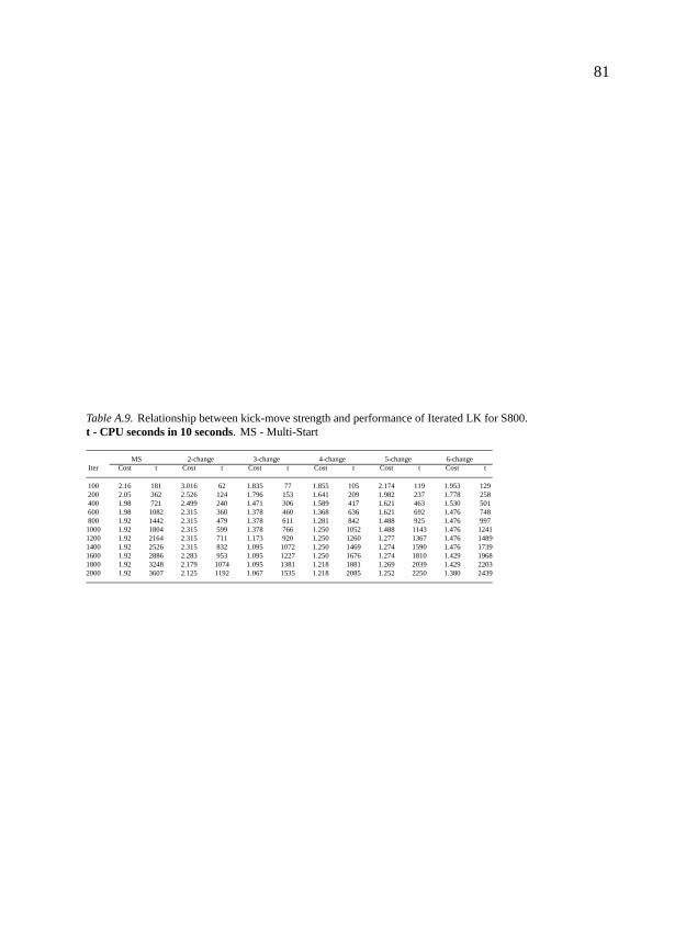
Table A.9.Relationship between kick-move strength and performance of Iterated LK for S800.t - CPU seconds in 10 seconds. MS - Multi-Start
MS 2-change 3-change 4-change 5-change 6-changeIter Cost t Cost t Cost t Cost t Cost t Cost t
100 2.16 181 3.016 62 1.835 77 1.855 105 2.174 119 1.953 129200 2.05 362 2.526 124 1.796 153 1.641 209 1.982 237 1.778 258400 1.98 721 2.499 240 1.471 306 1.589 417 1.621 463 1.530 501600 1.98 1082 2.315 360 1.378 460 1.368 636 1.621 692 1.476 748800 1.92 1442 2.315 479 1.378 611 1.281 842 1.488 925 1.476 9971000 1.92 1804 2.315 599 1.378 766 1.250 1052 1.488 1143 1.476 12411200 1.92 2164 2.315 711 1.173 920 1.250 1260 1.277 1367 1.476 14891400 1.92 2526 2.315 832 1.095 1072 1.250 1469 1.274 1590 1.476 17391600 1.92 2886 2.283 953 1.095 1227 1.250 1676 1.274 1810 1.429 19681800 1.92 3248 2.179 1074 1.095 1381 1.218 1881 1.269 2039 1.429 22032000 1.92 3607 2.125 1192 1.067 1535 1.218 2085 1.252 2250 1.380 2439