Implementation of Multigrid for Aerodynamic Computat ions on

Muiti-Block Grids

Luis Manzano

A thesis submitted in conformity with the requirements for the degree of Master of Applied Science

Graduate Department of Aerospace Science and Engineering University of Toronto

@ Copyright by Luis Manzano 1999

National Library 1+1 of Canada Bibliothèque nationale du Canada

Acquisitions and Acquisitions et Bibliographie Services services bibliographiques 395 Wellington Street 395, rw Wellington OItewaON KlAON4 OttawaON K 1 A W Canada Canada

Your bb Votre nnmca

Our lï& NNre réHnnru,

The author has granted a non- L'auteur a accordé une licence non exclusive licence allowing the exclusive permettant a la National Library of Canada to Bibliothèque nationale du Canada de reproduce, loan, distribute or sel1 reproduire, prêter, disîribuer ou copies of ths thesis in microform, vendre des copies de cette thèse sous paper or electronic fonnats. la forme de microfiche/film, de

reproduction sur papier ou sur format électronique.

The author retains ownership of the L'auteur conserve la propriété du copyright in this thesis. Neither the droit d'auteur qui protège cette thèse. thesis nor substantial extracts fiom it Ni la thèse ni des extraits substantiels may be printed or otherwise de celle-ci ne doivent être imprimés reproduced without the author's ou autrement reproduits sans son permission. autorisation.

Abstract

Implementation of Multigrid for

Aerodynarriic Computations on

Multi-Block Grids

Luis Manzano

Master of .4pplied Science

Graduate Department of Aerospace Science and Engineering

University of Toronto

1999

A multigrid algorithm to accelerate the convergence of the computation of compressible

aerodynamic flows on multi-block grids is presented. The diagonal form of an approximately-

factored time-marching method is ernployed in each block to advance the solution to stcady

state. Block interfaces are treated by overlapping the blocks by one cohmn of points and

using halo points. In the multigrid cycle, there is communication betwcen blocks at al1

levels. Turbulent viscosity is calculated using the S palart- Allmaras turbulerice rnodel. A

wide variety of tests are studied, including inviscid flows around single airfoils for C-rnesh

and H-me& topologies. Two multi-element test cases are investigated. the NLR-7301 airfoil

and flap. and case A-2 fiom the AGARD Advisory Report No. 303. Good performance is

shown in al1 test cases. Compared to the singlegrid solver, multigrid converges to steady

state in one-third to one-sixth the time.

iii

Acknowledgernent s

1 would like to thank the following individuals who made significant contributions to this

research:

Professor Zingg for his excellent guidance and supervision throughorit my research.

Doctor Nelson for his help with the TORNADO solver, patience and excellent teaching

on CFD.

Todd Chisholm for his multigrid explanations.

Stan De Rango for his help with SC1, TOmADO ...

Jason Lassaline for proof-reading my thesis and help wit h multigrid and Latex.

The rest of the CFD group for their Friendship, good humour and support.

My girlfriend and my parents for being so supportive, understanding and motivating.

Mike Sullivan for putting up with al1 the network technical problems.

Lurs MANZANO

University of Toronto

Ja~iuary 20, 1999

Contents

List of Figures ix

List of Symbols xi

1 Introduction 1 . . . . . . . . . . . . . . . . . . . . . . . . . . . . . . . . . . . . 1.1 Background 1

1.2 Project Definition and Objectives . . . . . . . . . . . . . . . . . . . . . . . . 2

2 Governing Equations and Numerical Met hod 3 . . . . . . . . . . . . . . . . . . . . . . 2.1 Thin-Layer Navier-Stokes Equations 3

. . . . . . . . . . . . . . . . . . . . . . . . . . . . . . . 2.2 Numerical Algorithm 4

. . . . . . . . . . . . . . . . . . . . . . . . . . . . . . . 2.3 Boundary Conditions 6 . . . . . . . . . . . . . . . . . . . . . 2.3.1 Far-field Boundary Conditions 7

. . . . . . . . . . . . . . . . . . . . . . . 2.3.2 Wall Boundary Conditions 7 . . . . . . . . . . . . . . . . . . . . . . . . . . . 2.3.3 Interface Conditions 8

. . . . . . . . . . . . . . . . . . . . . . . . . . 2.4 Treatment of Singular Points 9 . . . . . . . . . . . . . . . . . . . . . 2.4.1 Treatment of the Leading Edge 9 . . . . . . . . . . . . . . . . . . . . . 2.4.2 Treatment of the Trailing Edge 9

. . . . . . . 2.5 Spalart-Allmaras Turbulence Mode1 and the Multigrid Method 9

3 Multigrid 13 . . . . . . . . . . . . . . . . . . . . . . . . . . . . . . 3.1 The Multigrid Concept 13

. . . . . . . . . . . . . . . . . . . . . . . . . . . . . . . . . 3.2 MultigridCycles 14 . . . . . . . . . . . . . . . . . . . . . 3.3 Restriction and Prolongation Transfers 20

. . . . . . . . . . . . . . . . . . . . . . . . . . . . . . . . 3.3.1 Restriction 20 . . . . . . . . . . . . . . . . . . . . . . . . . . . . . . . 3.3.2 Prolongation 20

. . . . . . . . . . . . . . . . . . . . . . . . . . . . 3.4 Multigrid and Multiblock 20

4 Results 23 . . . . . . . . . . . . . . . . . . . . . . . . . . . . . . 4.1 VaJidation Test Cases 23

. . . 4.1.1 Test Case 1: Cornparison of Single- and Multi-block Mdtigrid 23 . . . . . . . . . . . . . 4.1.2 Test Case 2: Inviscid Flow on a 3-Block Grid 24

. . . . . . . . . . . . . . . 4.1.3 Test Case 3: Inviscid Flow on an H-Mesh 25 . . . . . . . . . . . . . . . . . . . . . . . . . . . . . . 4.2 High-Lift Applications 29

vii

4.2.1 Test Case 4: NLR-7301 Airfoil and Flap . . . . . . . . . . . . . . . . 29 4.2.2 Test Case 5: Case A-2 frorn the Advisory Report No. 303 . . . . . . 37

5 Conclusions and Recornmendat ions

References

A Multigrid Pseudo-codes

viii

List of Figures

2.1 3-Block C-Mesh . . . . . . . . . . . . . . . . . . . . . . . . . . . . . . . . . . 7 2.2 2-Block Grid with Halo Data . . . . . . . . . . . . . . . . . . . . . . . . . . 10

. . . . . . . . . . . . . . . . . . . . . . . . . . . . . 2.3 Leading Edge Treatment 11

. . . . . . . . . . . . . . . . . . . . . . . . . . . . . 2.4 Trailing Edge Treat rnent 11 2.5 Blunt Trailing Edge Treatment . . . . . . . . . . . . . . . . . . . . . . . . . 12

. . . . . . . . . . . . . . . . . . . . . . . . . . . 3.1 1D Illustration of Multigrid 14 . . . . . . . . . . . . . . . . . . . . . . . . . . . . . 3.2 2 Level Sawtooth Cycle IS

. . . . . . . . . . . . . . . . . . . . . . . . . . . . . . . . . . 3.3 Types of Cycles 19 . . . . . . . . . . . . . . . . . . . . . . . . . . . . . . . . . . . 3.4 Full-multigrid 20

. . . . . . . . . . . . . . . . . . . . . . . . . . . . . . . 3.5 Weighted Restriction 21 . . . . . . . . . . . . . . . . . . . . . . . . . . . . . . . . . . . 3.6 Prolongat ion 21

. . . . . . . . . . . . . . . . . . . . . . . . 3.7 Global Multigrid (2 Level Cycle) 22

4.1 Close-up of 3-Block Grid (Case 1) . . . . . . . . . . . . . . . . . . . . . . . 4.2 3-level Sawtooth Cycle (Single block (SC1) vs Multiblock (TORNADO) ) . 4.3 Residual History of Case 2 with Different Sawtooth Cycles . . . . . . . . . . 4.4 Lift Convergence of Cage 2 Using 2 and 3 Level Sawtooth Cycles . . . . . .

. . . . . . . . . 4.5 Drag Convergence of Case 2 with Different Sawtooth Cycles . . . . . . . . . . . . . . . . 4.6 Residual History of Case 2 with Full-Multigrid

. . . . . . . . . 4.7 Residual History of Case 2 with Sawtooth, V and W Cycles

. . . . . . . . . 4.8 Lift Convergence of Case 2 with Sawtooth, V and W Cycles . . . . . . . . . . . . . . . . . . . . . . . . . . . . . 4.9 Close-up of Case 2 Grid

4.10 Residual History of Case 3 Using a Sawtooth Cycle . . . . . . . . . . . . . . 4.1 1 Lift Convergence of Case 3 Using a Sawtooth Cycle . . . . . . . . . . . . . .

. . . . . . . . . . . . . . . . 4.12 Residual History of Case 3 Using Full-Multigrid 4.13 Residual History of Case 3 with Sawtooth, V and W Cycles . . . . . . . . . 4.14 Lift Convergence of Case 3 with Sawtooth. V and W Cycles . . . . . . . . . 4.15 Close-up of the NLR-7301 Grid . . . . . . . . . . . . . . . . . . . . . . . . . 4.16 Residual History of the NLR-7301 Case with a Sawtooth Cycle . . . . . . . 4.17 Residual History of the NLR-7301 Case with a Sawtooth Cycle (in Muitigrid

. . . . . . . . . . . . . . . . . . . . . . . . . . . . . . . . . . . . . . Cycles) 4.18 Lift Convergence of the NLR-7301 Case with a Sawtooth Cycle . . . . . . .

. . . . . . 4.19 Drag Convergence of the NLR-7301 Case with a Sawtooth Cycle 4.20 Residual History of the NLR-7301 Case with a Sawtooth. V and W Cycles . 4.21 Lift Convergence of the NLR-7301 Case with a SawtoothJ and W Cycles . 4.22 Drag Convergence of the NLR-7301 Case with a Sawtooth. V and W Cycles 4.23 Close-up of the A-2 Grid . . . . . . . . . . . . . . . . . . . . . . . . . . . . . 4.24 Residual History of A-2 Case with a Sawtooth Cycle . . . . . . . . . . . . . 4.25 Residual History of A-:! Case with a Sawtooth Cycle (in Multigrid Cycles) .

. . . . . . . . . . . 4.26 Lift Convergence of the A-2 Case with a Sawtooth Cycle . . . . . . . . . . 4.27 Drag Convergence of the A-2 Case with a Sawtooth Cycle

. . . . . . . . 4.28 Residual History of A-2 Case with Sawtooth. V and W Cycles 4.29 Residual History of A-2 Case with Sawtooth. V and W Cycles (in Multigrid

. . . . . . . . . . . . . . . . . . . . . . . . . . . . . . . . . . . . . . Cycles) . . . . . 4.30 Lift Convergence of the A-2 Case with Sawtooth. V and W Cycles

. . . . 4.31 Drag Convergence of the A-2 Case withsawtooth. V and W Cycles

List of Symbols

flux Jacobian matrices curvilinear convective flux vectors viscous flux Jacobian rnetric Jacobian Mach niirnber Praridt 1 number turbulent Prandt 1 number curvilinear state vector Reynolds number viscaus flw vector eigenvector matrix contravariant veloci ties rnolecular viscosity eddy viscosity

p density a speed of sound e total energy p pressure u, v Cartesian velocities h time step Ho total enthalpy

< curvilinear coordinat es

Qo rnultigrid initial solution vector Q mult igrid working solution vector Q+ mult igrid corrected solution vector P forcing function

RESTRCT restrict SMOOTH perform one iteration PLNG prolong RHS right hand side

Chapter 1

Introduction

1.1 Background

In computational fluid dynamics there are many aspects that must be considered

when solving the Navier-Stokes equations. It is important to consider the robustness. ac-

curacy and computat iorial expense of the algorit hm employed. grid generat ion and physical

nature of the flow. One important aspect which is considered here is the convergence rate

for steady flows.

Early efforts on the development of efficient solvers concentrated on approximate

factorization methods and methods of exploiting multigrid in some manner. Beam and

Warrning [l] introduced the approximate factorization method for the Euler and Navier-

Stokes equations in 1976. Steger [2] used this algorithm in the well known flow solver

ARCZD, which was further developed by Pulliam (31. ARC2D is an approximately-factored

implicit algorithm that uses centered spatial differences with artifiçial dissipation to solve

the Navier-Stokes equations.

Multigrid acceleration techniques were extended to the Euler equat ions by Jame-

son [4] [5], and to the Navier-Stokes equations by Martinelli et al. [6]. Jameson's approach

includes an explicit multi-stage iterative method, local time-stepping, and i~nplicit residual

smoot hing [7]. Caughey et al. [8] [9] [IO] extended multigrid to an approximately-factored

implicit multi-block algorit hm to solve the Euler equations. Chisholm [Il] applied a multi-

grid technique to the ARC2D solver in 1997. Chisholm and Caughey found that multi-

grid accelerated the convergence to steady state approximately by factors of 4 and 3.2,

respect ively. Jespersen, et al. [12] added mult igrid t o OVERFLOW, a t hree-dimensional

2 Chapter 1. Introduction

multiblock Navier-Stokes solver. Their results show speed-ups by a factor of 4 when using

multigrid.

When solving the Navier-Stokes equations over complex geometries, there are dif-

ficulties in generating smooth meshes. In order to overccme this obstacle, two basic ap-

proaches have been ptoposed. The first is to employ unstructured meshes as in methods

described by Jameson [4]. The second approach involves the use of multiblock strtictured

grids as in methods presented by Thompson [13]. This approach divides the flow-domain

into sub-domains or blocks. In each of these blocks, a structured mesh can be gcnerated

independently. Nelson 1141 [15] [16] developed a Navier-S tokes multiblock solver. known as

TORNADO (University of Toronto multi-block NAvier-stokes two Dimensional solver).

This code is an extension of ARC2D to rnultiblock grids. TORNADO is used to anal-

yse high-lift fiows over multi-element airfoils, which are necessary for take-off and landing

(see [17]).

1.2 Project Definition and Objectives

The objective of this project is to extend Chisholm's multigrid methodology to the

Spalart-Allmaras turbulence model (previously the Baldwin-Lomax model was used) and

to the TORNADO multi-block flow solver to speed-up its convergence rate.

Chapter 2

Governing Equations and

Numerical Method

The multigrid technique will be introduced in Chapter 3. First, the Navier-Stokes

equations and a description of the numerical algorithm used in TORNADO are presented.

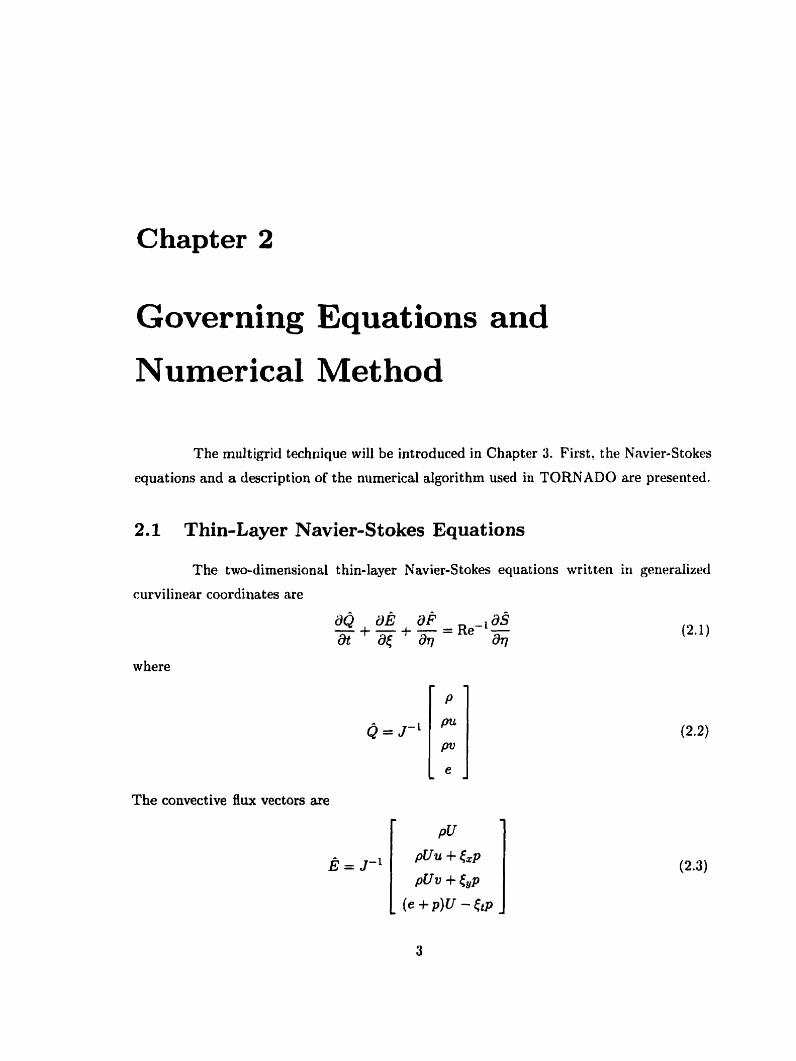
2.1 Thin-Layer Navier-Stokes Equations

The two-dimensional thin-layer Navier-Stokes equations written in generalized

curvilinear coordinates are

where

The convective flux vectors are

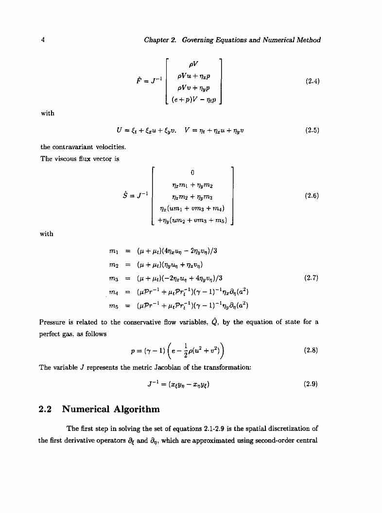
Chap ter 2. Gcrverning Equa tions and Numerical Method

with

the cont ravariant veiocities.

The viscoiis flux vector is

with

Pressure is related to the conservative flow variables, Q, by the equation of state for a

perfect gas, as follows

The variable J represents the metric Jacobian of the transformation:

2.2 Numerical Algorit hm

The b s t step in solving the set of equations 2.1-2.9 is the spatial discretization of

the first derivative operators aç and a,? which are approximated using second-order central

Section 2.2. Numerical Algori thm 5

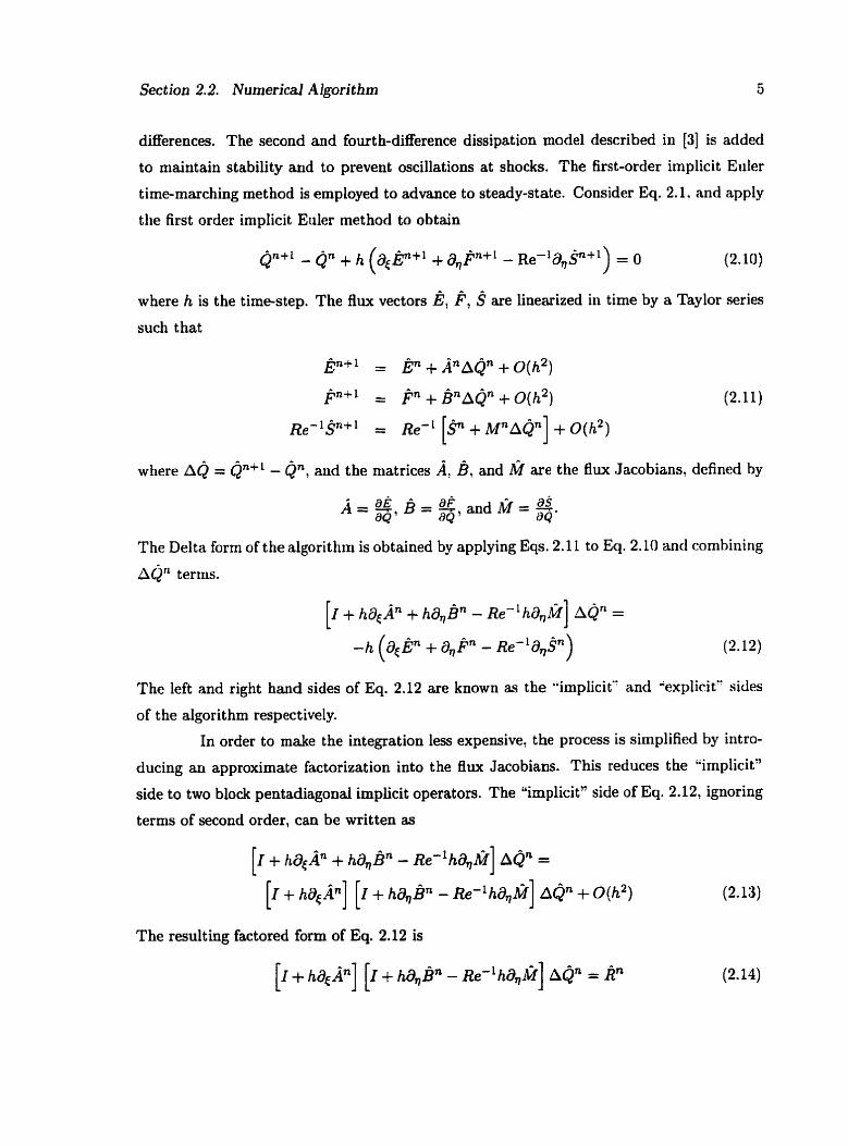
differences. The second and fourth-dinerence dissipation mode1 described in [3] is added

to maintain stability and to prevent oscillations at shocks. The first-order implicit Euler

time-marching method is employed to a d w c e to steady-state. Consider Eq. 2.1. and apply

the first order implicit Euler method to obtain

where h is the timestep. The flw vecton Ê, &', s are linearized in time by a Taylor series

such t hat

where AQ = Qn+' - Qn, and the matrices Â, B, and M are the flux Jacobians, defined by

The Delta form of the algorithin is obtained by applying Eqs. 2.11 to Eq. 2.10 ancl combining

hon terms.

The left and right hand sides of Eq. 2.12 are known as the "implicit" and -'expIicit2 sides

of the algorit hm respect ively.

In order to make the integration less expensive, the process is simplified by intro-

ducing an approximate factorization into the flux Jacobians. This reduces the "implicit"

side to two block pentadiagonal implicit operators. The "implicit" side of Eq. 2.12, ignoring

terms of second order, can be written as

The resulting factored form of Eq. 2.12 is

6

w here

Chapter 2. Governing Eq uations and Numericd Me thod

The computational work required for the inversion of the "implicit" side can be further

reduced by introducing a diagonalization of the implicit blocks. The flux Jacobians  and

B can be diagoaalized as

where TE and T, are matrices whose colurnns are the eigenvectors of the flux Jacobians A

and b respectively. Applying Eqs. 2.16 to the factored form Eq. 2.14 gives

where Rn is the right hand side of Eq. 2.14. The following equation results by factoring the

Tc and T, eigenvector matrices outside the spatial derivatives û.. and 8,.

where N = T c 'T,. The viscous flux Jacobian M cannot be diagonalized with B. An

approximation to the viscous .Tacobian eigenvalues is introduced to the left hand side of

Eq. 2.18 (set: [3]).

The rate of convergence can also be increased by using local tirne stepping. This

is obtained by scaling the time step with the Jacobian of the coordinate transformation.

2.3 Boundary Conditions

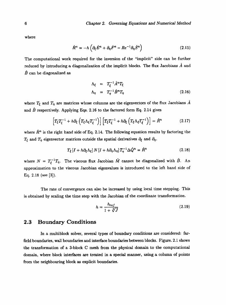
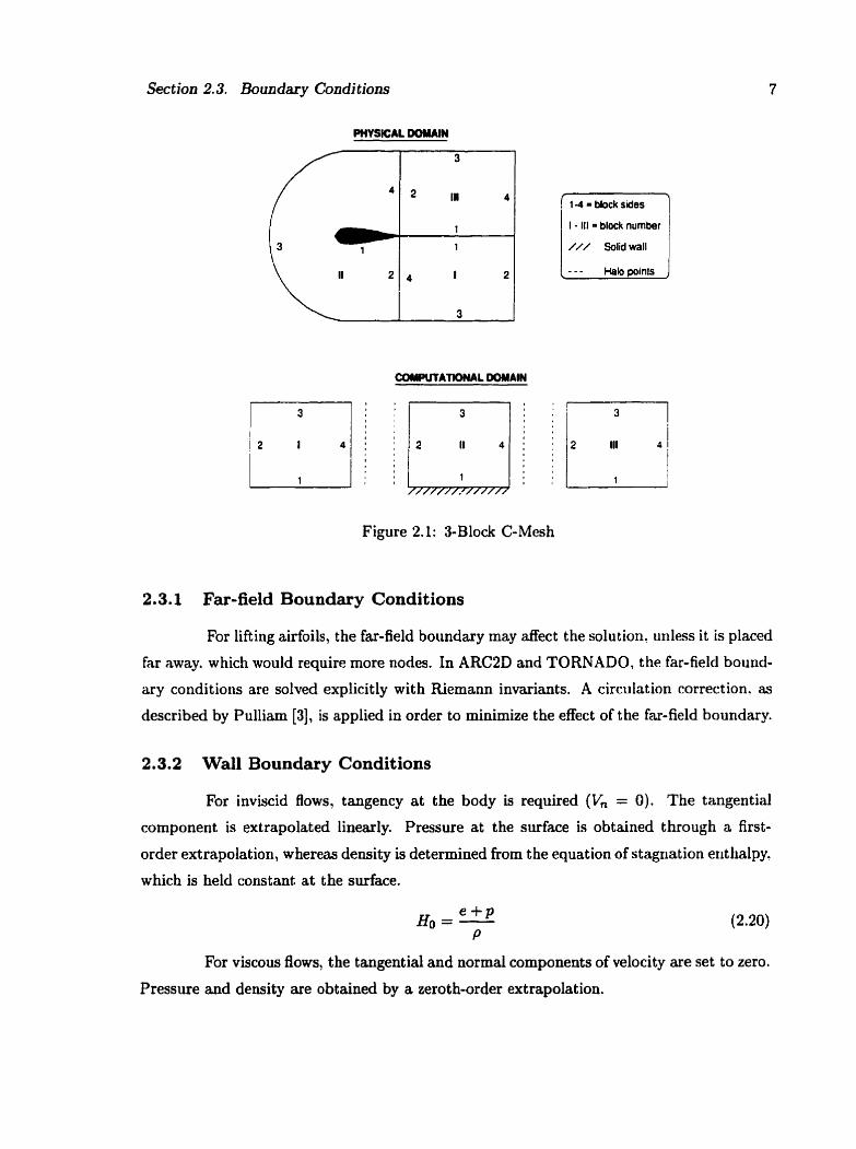
In a multiblock solver, several types of boundary conditions are considered: far-

field boundaries, wall boundaries and interface boundaries between blocks. Figure. 2.1 shows

the transformation of a 3-block C mesh from the physical domain to the computational

domain, where block interfaces are treated in a special manner, using a column of points

from the neighbouring block as explicit boundaries.

Section 2.3. Boundary Conditions

14 = block sides

I - 111 = block number I

Figure 2.1: 3-Block C-Mesh

2.3.1 Far-field Boundary Conditions

For lifting airfoils, the far-field boundary may affect the solution, unless i t is placed

far away. which would require more nodes. In ARC2D and TORNADO, the far-field bound-

ary conditions are solved explicitly with Riemann invariants. A circulation correction. as

described by Pulliam [3], is applied in order to minimize the effect of the far-field boundary.

2.3.2 Wall Boundary Conditions

For inviscid flows, tangency at the body is required (V, = O). The tangential

component is extrapolated linearly. Pressure at the surface is obtained through a first-

order extrapolation, whereas density is determined from the equation of stagriat ion ent halpy.

which is held constant a t the surface.

For viscous flows, the tangential and normal components of velocity are set to zero.

Pressure and density are obtained by a zeroth-order extrapolation.

8 Cbapter 2. Governing Eguations and Numerical Method

2.3.3 Interface Conditions

In TORNADO, the interface conditions are updated depending on the nature of

the block side. If the block side is in the 7 direction, they are obtained by overlapping

neighbouring blocks at the interface, and an extra column of points taken from the neigh-

boiiring block (known as the "halo" column) provides explicit boundary conditions. If the

block side is in the { direction, the interface is updated through a linear extrapolation of

the interior nodcs.

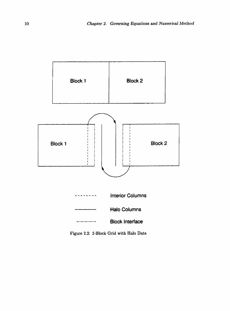
In order to explain the sequence of events when updating the interface conditions

iising "halo" columns, consider a rectangular Zblock grid (see Figure 2.2). The first interior

column of block 2 is stored in the "halo" column of block 1, and the last interior column of

block 1 is stored in the "halo" column of block 2. To advance a time-step, blocks 1 and 2 are

updated independently of one another, which causes two solutions at their interface. The

average of these two solutions is stored at the interface and the process is repeated until the

residual is driven to machine zero. The interface is completely transparent at steady state.

Consider now a case in which no "halo" points are used to update the houndaries.

Once the extrapolation from the interior points of both blocks has been performed. the

interface will store the average of the soiutions obtained from both blocks. With this

approach the interface is not transparent, even at steady state, and some degradation of

accuracy will occur.

Section 2.4. Zleatment of Singular Points

2.4 Treatment of Singular Points

In a multiblock solver, nodes which are shared by more than two blocks require

special consideration. These nodes, such as the leading edge or the trailing edge of an airfoil

can greatly affect the convergence of the solver, depending on how they are treated.

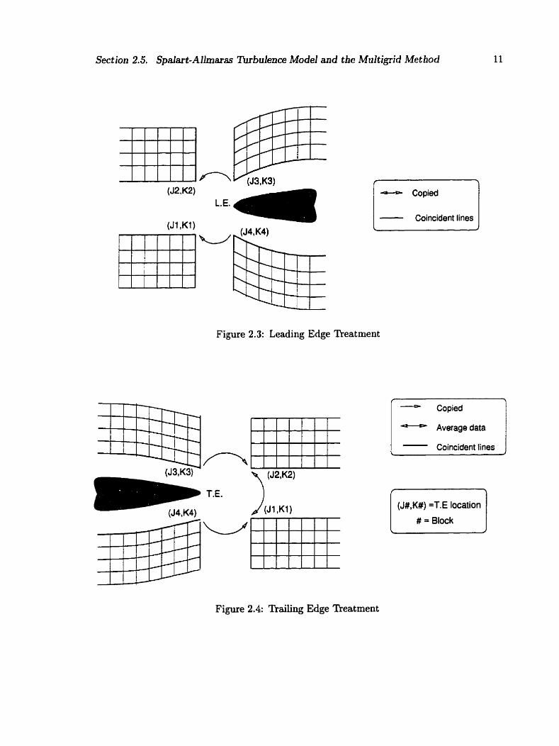
2.4.1 Treatment of the Leading Edge

The leading edge of the airfoil, as shown in Fig. 2.3 is shared by three or four

blocks, depending on the type of mesh (3 blocks for a C mesh, 4 blocks for a n H mesh).

From Fig. 2.3, it can be seen that (J3, K3) and (J4, K4) are copied to points ( . J 2 , K 2 ) and

( J I , KI) respectively. For viscous cases, the average of Ieading edge point on blocks 1 and

2 is stored in ( J I , K I ) and (52, K2)

2.4.2 Treatment of the Pailing Edge

The trailing edge of the body is handled in a manner similar to that of the leading

edge. As presented in Fig. 2.4, the trailitig edge points of the block having the body surface

in one of its sides are copied to the neighbouring block. The average of points (53, K3) and

(J4 : K4) is copied to ( J I , K l ) , (52, K2), (53, K3) and ( 5 4 , K4).

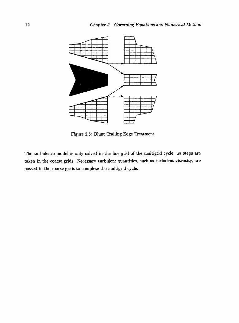
In the case of a blunt trailing edge, two ccjpies are made to the blocks behind the

airfoil as shown in Fig. 2.5

2.5 Spalart- Allmaras Turbulence Mode1 and the Multigrid

Method

The Spalart-Allmaras turbulence model [18] is a widely used one-equation model

(approximately-factored implicit algorithm). The turbulence mode1 is local (the equation

at one point does not depend on the solution at other points), and yields fairly rapid

convergence to steady-state. It is well suited for the phenomena that occur in the multi-

element case, such as flow separation and confluent boundaqy layers.

The turbulence model and the fiow solver are loosely coupled: take one step of

the turbulence model, take one step of the flow solver. The same approach is used with the

multigrid algorithm: one step of the turbulence model, one step of the multigrid algorithm.

Block 1

Chap ter 2. Governing Equa tions and Numericd Met hod

Block 1

Block 2

Interior Columns

Halo Columns

Block 2

-...--..-...--..- Block Interface

Figure 2.2: 2-Block Grid with Halo Data

Section 2.5. Spalart-Al1rniu'a.s îbrbulence Mode1 and the Multigrid Method

L.E.

u

Figure 2.3: Leading Edge

- Copied r - Coincident lines

I - Copied

- Coincident lines )

r

(J#,K#) =T.E location

# = Block

Figure 2.4: Trding Edge Treatment

Cbapter 2. Governing Equations and Numericd Met hod

Figure 2.5: Blunt Trailing Edge Treatment

The turbulence mode1 is only solved in the fine grid of the multigrid cycle, rio steps are

taken in the coarse grids. Necessary turbulent quantities, such as turbulent viscosity. are

passed to the coarse grids to complete the multigrid cycle.

Chapter 3

Mult igrid

3.1 The Multigrid Concept

Multigrid methods are used to accelerate the numerical solution of partial differen-

tial equations, such as the compressible Navier-Stokes equations. The essence of multigrid

methods is to use a family of discrete problems, defined in several grids, al1 approxinlat-

ing the same continuous problem, to help in the soIution of the large systems of equa-

tions (191 (201. The main purpo.se of the multigrid technique is to accelerate the solution by

removing low frequency errors. It was originally developed for elliptic differential equations.

Since then it has been applied to other type of systems, such as the Navier-Stokes equations.

When an iterative solver is applied to the spatially discretized equations, the resid-

ual is reduced until the steady solution is obtained. Solvers tend to reduce the error differ-

ently depending on its frequency. They are normally much better at reducing high frequency

errors. Consider an error of one frequency of a one-dimensional grid with uniforrn grid spac-

ing. If the error is passed to a coarser grid formed by the removal of every ot ber node of the

finer grid, its fiequency is doubled. Hence, the iterative solver wiIl remove this error more

quickly since it is of higher frequency. This is illustrated in Fig. 3.1, where a wave with 16

points per wavelength on the finest grid has a higher frequency (4 points per wavdength)

on the coarsest grid. This coarse grids are formed by the removal of every other node.

Hence, the fkequency has effectively been raised. The objective of the multigrid technique

is to reduce the low frequency error by using several grids to remove this type of error faster

than the conventional iterative solvers do by the use of one grid only. Thus, the effectiveness

of the multigrid technique depends largely on the capacity of the smoother to remove the

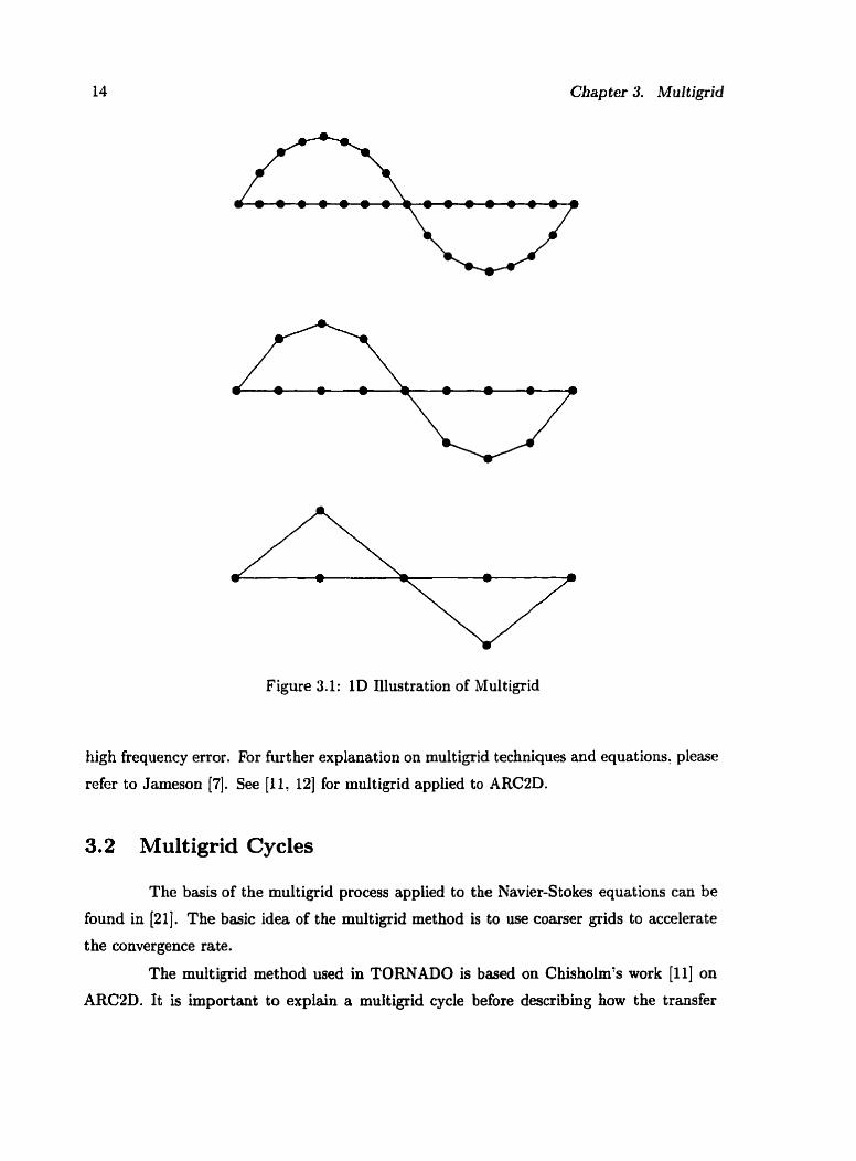
Chapter S. Multigrid

Figure 3.1: 1D Illustration of Multigrid

high frequency error. For furt her explanat ion on multigrid techniques and equations, please

refer to Jameson (71. See [I l , 121 for multigrid applied to ARC2D.

3.2 Multigrid Cycles

The basis of the multigrid process applied to the Navier-Stokes equations can be

found in [21]. The basic idea of the multigid method is to use coarser grids to accelerate

the convergence rate.

The multigrid method used in TORNADO is based on Chisholm's work [Il] on

ARC2D. It is important to explain a multigrid cycle before describing how the transfer

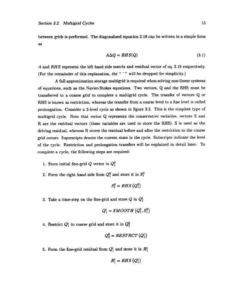
Section 3.2. Mul tigrid Cycles 15

between grids is performed. The diagonalized equation 2.18 can be written in a simple form

a4

AAQ = RHS(Q) (3.1)

.4 and RHS represent the left hand side matrix and residual vector of eq. 2.18 respectively.

(For the remainder of this explariation, the " " will be dropped for simplicity.)

A full approximation storage multigrid is required when solving non-linear systems

of equations, such as the Navier-Stokes equations. Two vectors, Q and the RHS must be

transferred to a coarse grid to complete a multigrid cycle. The transfer of vectors Q or

RHS is known as restriction, whereas the transfer from a coarse level to a fine level is caIled

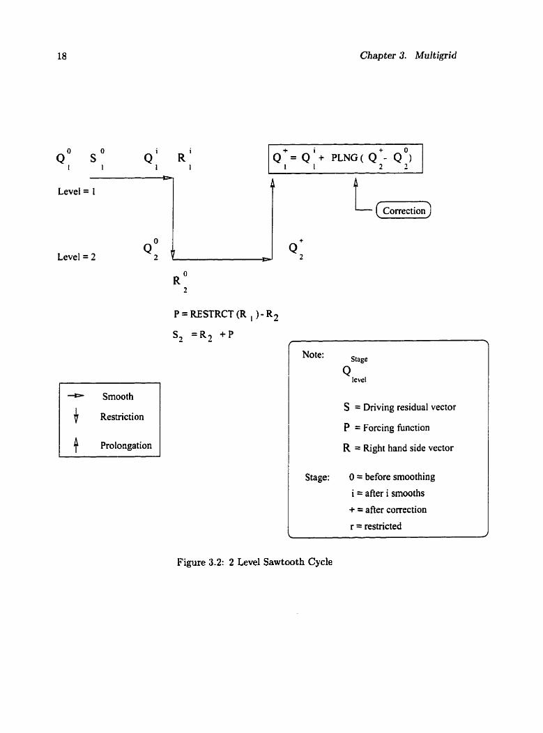
prolongation. Consider n 2-level cycle as shown in figure 3.2. This is the siniplcst type of

multigrid cycle. Note that vector Q represents the conservative variables. vectors S ancl

R are the residual vectors (these variables are used to store the RHS). S is used as the

driving residual, whereas R stores the residual before and after the restriction to the coarse

grid occurs. Superscipts denote the current state in the cycle. Subscripts indicate the level

of the cycle. Restriction and prolongation transfers will be explained in detail later. To

complete a cycle, the following steps are required:

1. Store initial fine-grid Q vector in QT

2. Form the right hand side from Qy and store it in Sy

S: = RHS (Q:)

3. Take a time-step on the fine-grid and store Q in ~f

4. Restrict Qf to coarse grid and store it in Q2

Q! = RESTRCT (Q:)

5. Form the fine-grid residual fiom ~f and store it in R:

Rf = RHS (QI)

Chapter 3. Multigrid

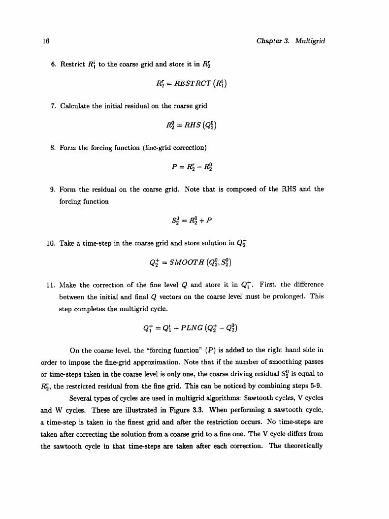
6. Restrict Ri to the coarse grid and store it in

R; = RESTRCT ( ~ f )

7. Calculate the initial residual on the coarse grid

= RHS (Q:)

8. Form the forcing function (fine-grid correction)

9. Form the residual on the coarse grid. Note that is composed of the RHS and the

forcing function

10. Take a time-step in the coarse grid and store solution in Qz

11. Make the correction of the fine level Q and store it in Q:. First? the diffcrence

between the initial and final Q vectors on the coarse level must be prolonged. This

step completes the multigrid cycle.

On the couse level? the "forcing function?' (P) is added to the right hand side in

order to impose the fine-grid approximation. Note that if the number of smoothing passes

or time-steps taken in the coarse level is only one, the coarse driving residualS2 is equal to

4, the restricted residual from the fine grid. This can be noticed by combining steps 5-9.

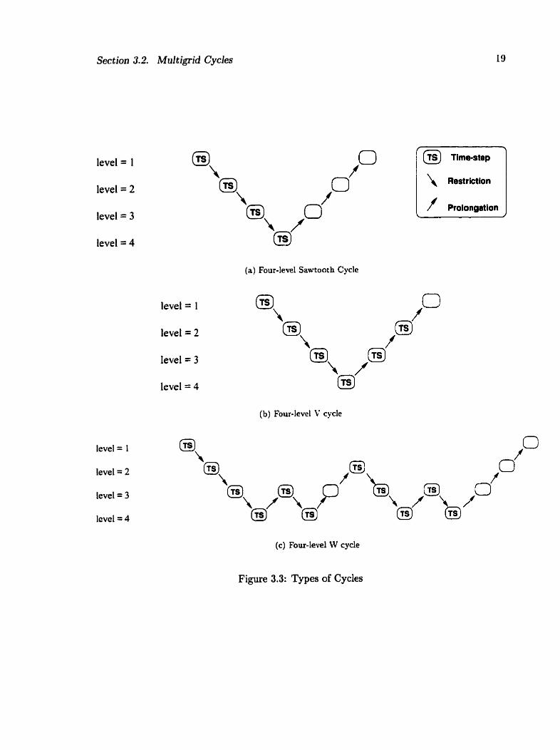
Several types of cycles are used in multigrid algorithms: Sawtoot h cycles, V cycles

and W cycles. These are illustrated in Figure 3.3. When performing a sawtooth cycle,

a time-step is taken in the finest grid and after the restriction occurs. No tirne-steps are

taken after correcting the solution fiom a coarse grid to a fine one. The V cycle d8ers from

the sawtooth cycle in that time-steps are taken &er each correction. The theoretically

Section 3.2. Multigrid Cycles 17

best cycle is the W-cycle, where more time is spent on the coarse levels. The coarse grid

correctio~is are smoothed before they are transferred back to the finest level.

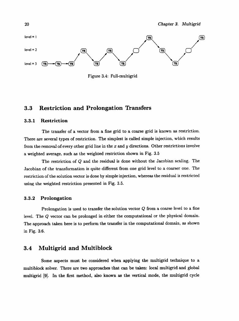
Grid sequencing is also widely used to accelerate the convergence of the solver. In

aerodynamic flows, the conservative variables are initialized to the free stream condit ions.

Grid sequencing provides a better initial guess. Several iterations are taken in a coarse level

and then the Q vector is transferred to the desired grid. The combination of this technique

with multigrid is known as full-multigrid. Figure 3.4 shows a 3-level full-miiltigrid, in which

some iterations are taken in the coarse grids before the solution is transferred to the finest

grid. In levels 2 and 1, the multigrid algorithm is applied.

A large part of the time required to perform a multigrid cycle is spent calculating

the RHS (it is calculated twice to form the forcing function), and performing the restriction

and prolongation transfen (see [Il]). One way to reduce the ntiinber of RHS calculations

and transfers is to perfor~n several iterations in each multigrid level. As cz resiilt. the

multigrid cycle becornes more efficient, and the CPU time required to converge to machine

zero is reduced significantly. Some caution should be taken: performing too niariy sinooths

per level can reduce the effectiveness of the rnultigrid cycle. In TORNADO. the optimal

number of smooths per level is 4.

Chapter 3. Multigid

Level = 2

- Smooth

6 Restriction

1 i\ Prolongation

P = RESTRCT (R , ) - R2 S, = R 7 - + P

Note: Stage

Q level

S = Driving residual vector

P = Forcing function

R = Right hand side vector

Stage: O = before smoothing

i = aAer i smooths

+ = aAer correction

r = restricted

Figure 3.2: 2 Level Sawtooth Cycle

Section 3.2. Mu1 tigrid Cycles

level = 1

level = 2

level = 3

level = 4

level = 1

level = 2

level = 3

level = 4

level = 1

level = 2

level = 3

level = 4

(a) Four-level Sawtooth Cycle

(b) hur-level V cycle

(c) Four-levei W cycle

Figure 3.3: Types of Cycles

lcvel= 1

level = 2

Icvel = 3

Figure 3.4: Full-multigrid

3.3 Restriction and Prolongation Transfers

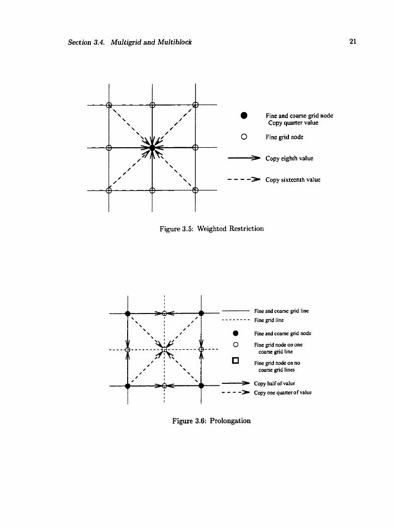
3.3.1 Restriction

The transfer of a vector from a fine grid to a coarse grid is known as restrictiori.

There are several types of restriction. The simplest is cdled simple injection, which results

from the rernoval of every ot her grid line in the x and y directions. Other restrictions involve

a weighted average, such as the weighted restriction shown in Fig. 3.5

The restriction of Q and the residuai is done without the Jacobian scaling. The

Jacobian of the transformation is quite different from one grid level to a coarser one. The

restriction of the solution vector is done by simple injection, whereas the residual is restric ted

using the weighted restriction presented in Fig. 3.5.

3.3.2 Prolongation

Prolongation is used to transfer the solution vector Q fiom a coarse level to a fine

level. The Q vector can be prolonged in either the computational or the physical domain.

The approach taken here is to perform the transfer in the computational domain, as shown

in Fig. 3.6.

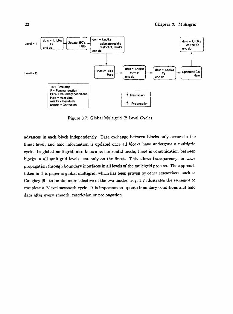
3.4 Multigrid and Multiblock

Some aspects must be considered when applying the multigrid technique to a

multiblock solver. There are two approaches that can be taken: local multigrid and global

rnultigrid [9]. In the iirst method, algo known as the vertical mode, the multigid cycle

Section 3.4. Muldigrid and Multiblock

Fine and coarse grid node Copy quarter value

0 Fine grid node - Copy eighth value

---- > Copy sixtecnth value

Figure 3.5: Weighted Restriction

1 1

A. Fine and coarsc grid line . C ' I - - * * - - - - \ 1 # Fine grid line \ 1 # \ I 0

\ l ) Fine and coarse grid nodc '\ : '

- - - * - - - - - - - - - - - ,x 0 Fine grid node on one coarse grid line

# ' \ 0 1 \ Fine grid node on no

/ 1 1

\ coarse grid lines , \ \ \

dL Copy haIf of value v I - - - - * Copy one qtuner of value

Figure 3.6: Prolongation

Chap ter 3. Muftigrid

\ - 1 end do 1

r r -?

Level = 2

Level = 1

Ts = Tme step P = forcing function BC's = Boundary conditions Halo = Halo data resid's = Residuals correct = Correction

do n = 1,nblks Ts , Update: BC's caladate resid's

end do Halo restrict Q, resid's

1 Restriction

t Prolongation

1 f r I

Figure 3.7: Global Multigrid (2 Level Cycle)

do n = 1 ,nblks Update: BC's

form P Halo -

advances in each block independently. Data exchange between blocks only occurs in the

finest level, and halo information is updated once al1 blocks have undergone a multigrid

cycle. In global multigrid, also known as horizontal mode, there is cornunication between

blocks in al1 multigrid levels. not only on the finest. This allows transparency for wave

propagation t hrough boundary interfaces in al1 levels of the multigrid process. The approach

taken in this paper is global rnultigrid, which has been proven by other researchers, such as

Ca~igliey [9]. to be the more effective of the two modes. Fig. 3.7 illustrates the sequence to

cornplete a Slevel sawtooth cycle. It is important to update boundary conditions and halo

data after every smooth, restriction or prolongation.

k J end do c end do Halo r L I

r 7 f 5 - do n = 1 ,nblks Ts ,, Update: BC's

Chapter 4

Results

This chapter is divided into validation test cases and high-lift applications. Invis-

cid cases are studied to validate the multigrid algorithm for a single-element airfoil. The

multigrid-mult iblock algorit hm is also compared to the single block solver SC 1 and wit h

multigrid. In the high-lift section, the cases considered include a fully-attached flow over

the NLR-7301 airfoil and flap, and case A2 from the AGARD Advisory Report No.303.

A Silicon Graphics Origin 200 machine was used to run al1 test cases. The flags user1 to

compile the code were 0 3 and mips4. The effectiveness of the sawtoot h, V and W cycles is

studied. In al1 test cases, four iterations are performed on al1 multigrid levels.

4.1 Validation Test Cases

4.1.1 Test Case 1: Cornparison of Single- and Multi-block Multigrid

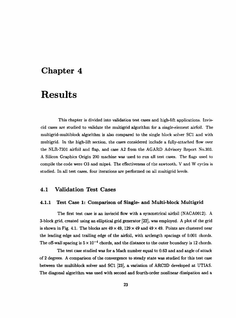
The first test case is an inviscid flow with a symmetrical airfoil (NACA0012). A

3-block grid, created using an elliptical grid generator [22], was employed. A plot of the grid

is shown in Fig. 4.1. The blocks are 49 x 49, 129 x 49 and 49 x 49. Points are clustered near

the leading edge and traiiing edge of the airfoil, with arclength spacings of 0.001 chords.

The off-wall spacing is 5 x 1 0 - ~ chords, and the distance to the outer boundary is 12 chords.

The test case studied was for a Mach nurnber equal to 0.63 and and angle of attack

of 2 degrees. A cornparison of the convergence to steady state was studied for this test case

between the multiblock solver and SC1 [23], a miation of ARC2D developed at UTIAS.

The diagonal algorithm was used with second and fourth-order nonlinear dissipation and a

Chapter B. Results

Figure 4.1: Close-up of 3-Block Grid (Case 1)

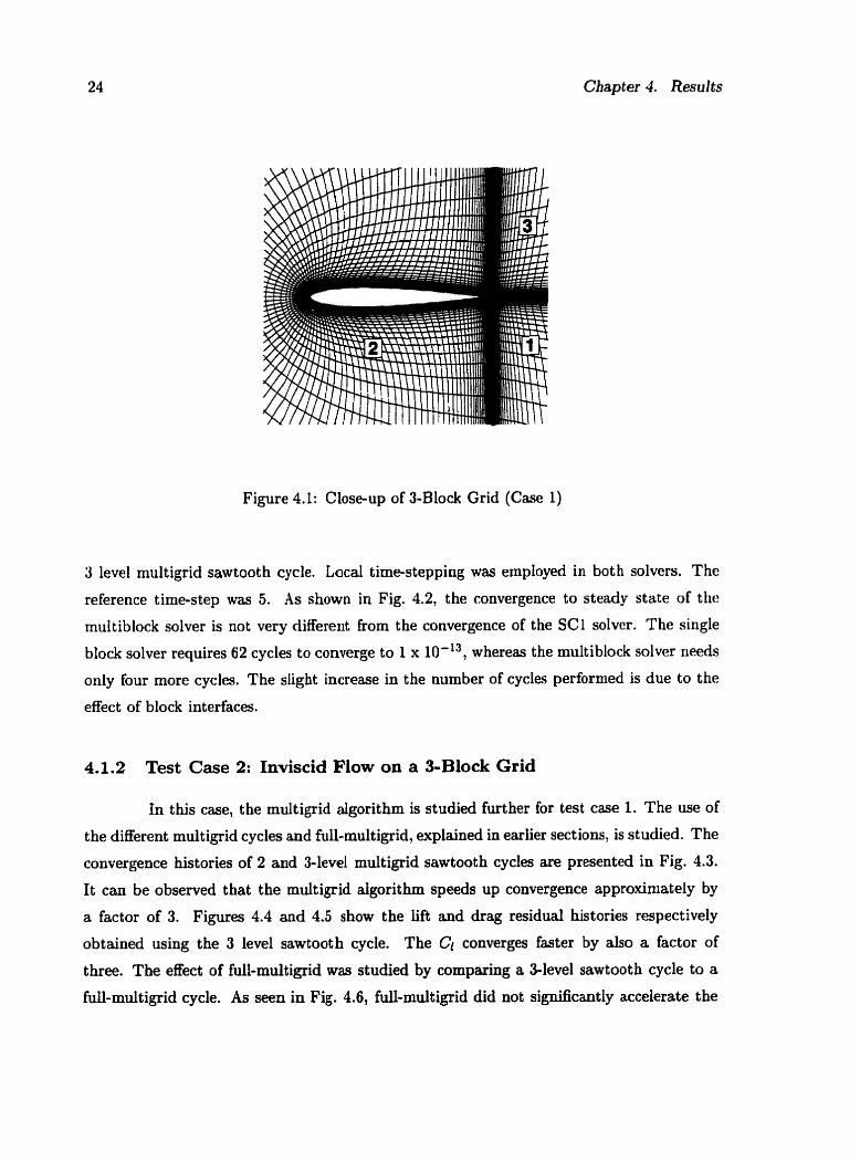
3 level multigrid sawtooth cycle. Local time-stepping was employed in bot h solvers. The

reference tirne-step was 5. A s shown in Fig. 4.2, the convergence to steady state of tlic

multiblock solver is not very different from the convergence of the SC1 solver. The single

block solver requires 62 cycles to converge to 1 x 1 0 - ~ ~ , whereas the multiblock solver needs

only four more cycles. The slight increase in the number of cycles performed is due to the

effect of block interfaces.

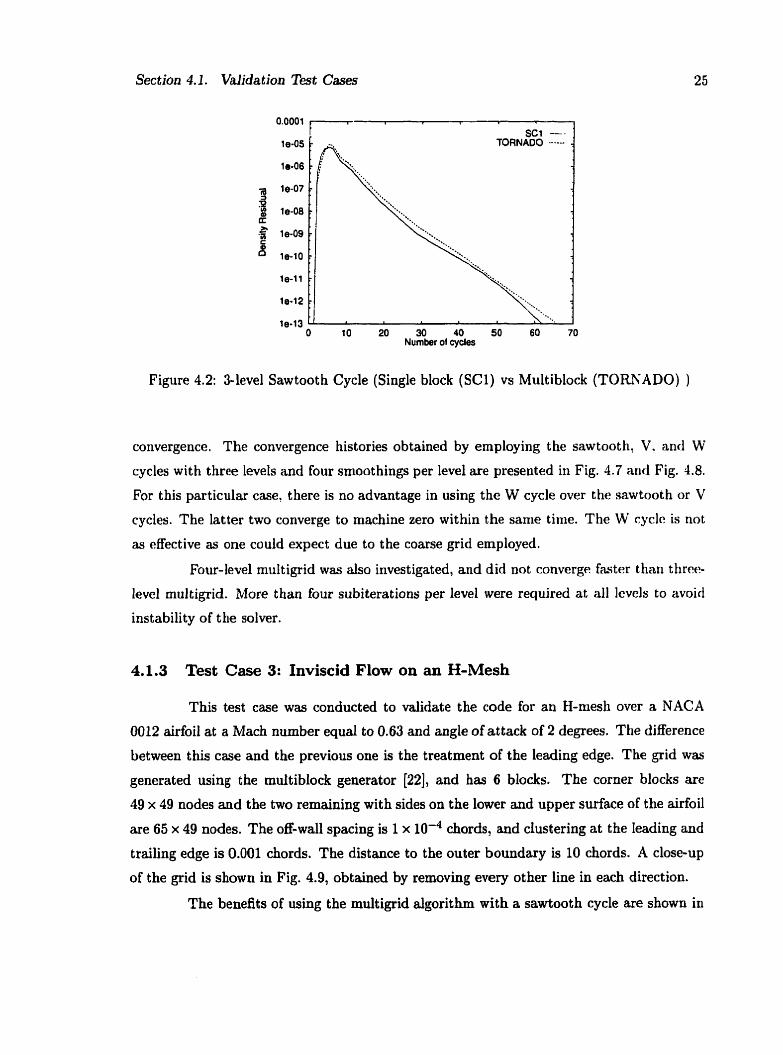
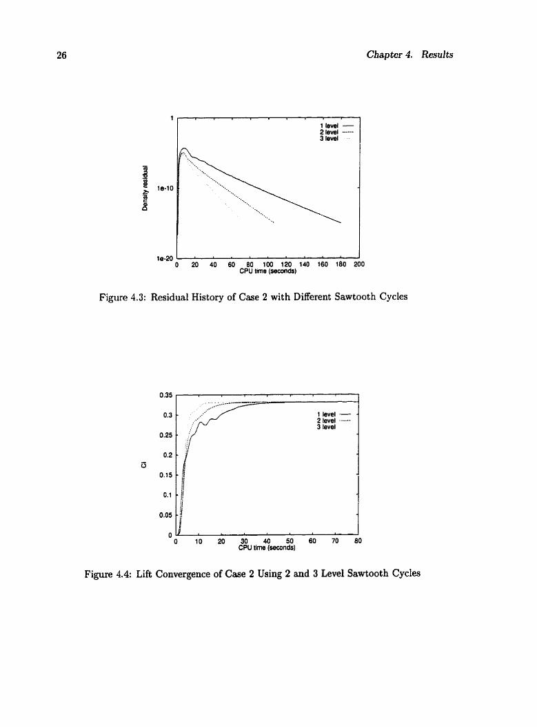
4.1.2 Test Case 2: Inviscid Flow on a 3-Block Grid

In this case, the multigrid algorithm is studied further for test case 1. The use of

the different mult igrid cycles and full-multigrid, explained in earlier sections, is st udied. The

convergence histories of 2 and 3-level multigrid sawtooth cycles are presented in Fig. 4.3.

It can be observed that the multigrid aigorithm speeds up convergence approximately by

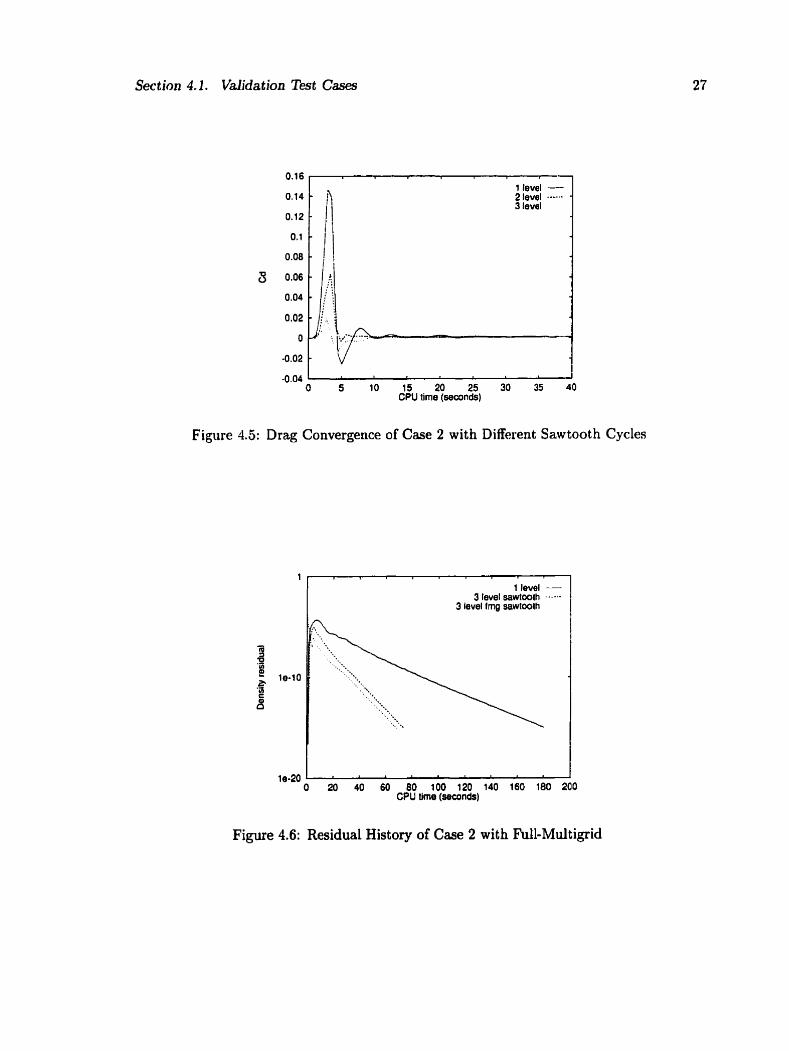
a factor of 3. Figures 4.4 and 4.5 show the lift and drag residual histories respectively

obtained using the 3 level sawtooth cycle. The Ci converges faster by also a factor of

three. The effect of full-multigid was studied by cornparhg a 3-level sawtooth cycle to a

full-multigrid cycle. As seen in Fig. 4.6, füU-multigrid did not significantly accelerate the

Section 4.1. Validation Test Cases

Number of cycles

Figure 4.2: 3-level Sawtooth Cycle (Single block (SC1) vs Multiblock (TORNADO) )

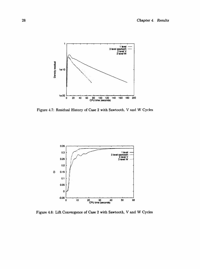
convergence. The convergence histories obtained by ernploying the sawtoot h, V1 and W

cycles with three levels and four smoothings per level are presented in Fig. 4.7 arid Fig. 3.8.

For this particular case, there is no advantage in using the W cycle over the sawtooth or V

cycles. The latter two converge to machine zero within the sanie tinie. The W cyclc is not

as effective as one could expect due to the coarse grid ernployed.

Four-level multigrid was also investigated, and did not converge faster t han thrce-

level multigrid. More than four subiterations per level were required at al1 levels to avoid

instability of the solver.

4.1.3 Test Case 3: Inviscid Flow on an H-Mesh

This test case was conducted to validate the code for an H-mesh over a NACA

0012 airfoil at a Mach number equal to 0.63 and angle of attack of 2 degees. The difference

between this case and the previous one is the treatment of the leading edge. The g i d was

generated using the muttiblock generator [22], and has 6 blodts. The corner blocks are

49 x 49 nodes and the two remaining with sides on the lower and upper surface of the airfoil

are 65 x 49 nodes. The off-wall spscing is 1 x 10-~ chords, and clustering at the leading and

trailing edge is 0.001 chords. The distaoce to the outer boundary is 10 chords. A close-up

of the grid is shown in Fig. 4.9, obtained by removing every other line in each direction.

The benefits of using the multigrid algorithm with a sawtooth cycle are shown in

Cbapter 4. Results

1 lewi - 2 level ----- 3 level , .

le-20 1 J O 20 40 60 80 100 120 140 160 180 200

CPU tirne (seconds)

Figure 4.3: Residual History of Case 2 with Different Sawtooth Cycles

. . .l__l*..---

0.3 1 level - 2 level ------ 3 level

0.25

O 10 20 30 40 50 60 70 80 CPU time (seconds)

Figure 4.4: Lift Convergence of Case 2 Using 2 and 3 Level Sawtooth Cycles

Section 4.2. Validation Test Cases

-0.04 1 O 5 10 15 20 25 30 35 40

CPU time (seconds)

Figure 4.5: Drag Convergence of Case 2 with Different Sawtooth Cycles

1 level - 3 revei sawtooth ------

3 level fmg sawtoolh

O 20 40 60 80 100 120 140 160 180 200 CPU time (seconds)

Figure 4.6: Residual History of Case 2 with Full-Multigrid

Cbapter 4. Results

1 ievei - 3 level sawtooth -----

3 level V 3 level W

19-20 O 20 40 60 80 100 120 140 160 160 200

CPU time (seconds)

Figure 4.7: Residual History of Case 2 with Sawtooth. V and W Cycles

I O 1 O 20 30 40 50 60

CPU tirne (seconds)

Figure 4.8: Lift Convergence of Case 2 with Sawtooth, V and W Cycles

Section 4.2. High-Lift Applications

Figure 4.9: CIose-up of Case 2 Grid

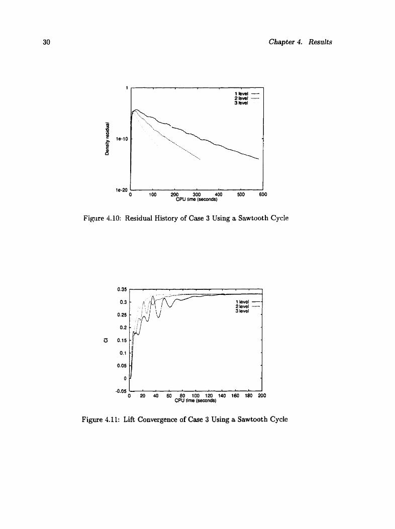
Fig. 4.10. There is a great speed-iip, approximately a factor of 6, when iising niiiIt,igid.

The Ci convergence rate also improves by a large factor, approximately 4 (see Fig. 4.1 1).

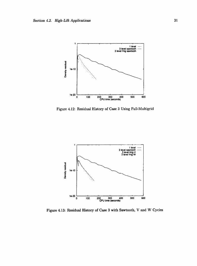
As in the previous test case? the use of full-multigrid contributes to a shorter riin tinie

(see Fig. 4.12). In this case, the W cycle proved to be the most effective. As shown in

Fig. 4.13, the W cycle had the best convergence rate, followed by the V cycle. Iri the V

cycle, four iterations were performed after each correction was made. In the case of the Cr,

the convergence of the W and V cycles is almost identicai, as shown in Fig. 4.14.

4.2 High-Lift Applications

4.2.1 Test Case 4: NLR-7301 Airfoil and Flap

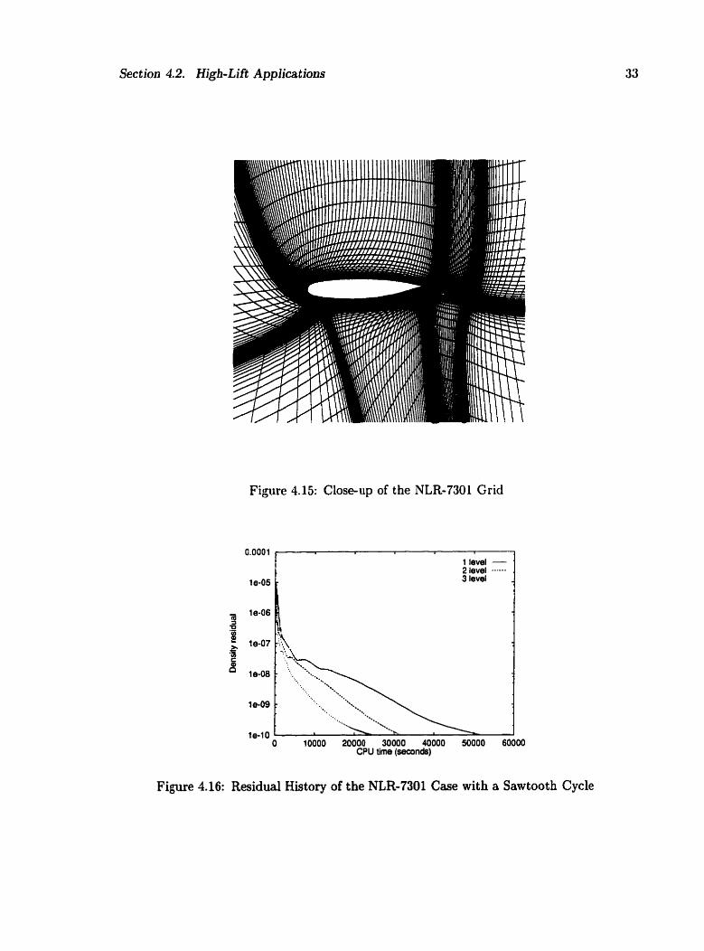
Tests were performed on the NLR-7301 airfoil and flap configuration previously

studied using TORNADO 1151, as shown in Fig. 4.15 (obtained by removing every other

line in each direction), which has a 32% chord flap with an angle of 20 deg. The overlap is

5.3% chord and the nominal gap setting is 2.4% chord. The Mach nurnber and the Reynolds

nurnber were 0.185 and 2.51 x 1CI6 respectively. The angle of attack was set at 13.1 deg,

Chapter 4. Resiilts

le-20 1 I O 100 200 300 400 500 600

CPU tirne (seconds)

Figure 4.10: Residual History of Case 3 Using a Sawtooth Cycle

0.35

1 level -- 2 level -- 3 level

-0.05 1 O 20 40 60 eo ioo 120 140 iso iao 200

CPU tirne (seconds)

Figure 4.11: Lift Convergence of Case 3 Using a Sawtooth Cycle

Section 4.2. Wgh- Lift Applications

t level - 3 level sawtooth ------

3 level fmg sawîwth

10-20 O 100 200 300 400 500 600

CPU time (seconds)

Figure 4.12: Residual History of Case 3 Using Full-Multigid

1 level - 3 level sawtaoth ------

3 level h g - V 3 level fmg-W

O 100 200 300 400 500 600 CPU tirne (seconds)

Figure 4.13: Residual History of Case 3 with Sawtooth, V and W Cycles

Chapter 4. Results

1 level - 3 level fmg-saw!oolh --

0.25 3 !evel fmg-V . . 3 leml fmg-w --

Figure 4.14: Lift Convergence of Case 3 with Sawtooth. V and W Cycles

0.2

0 0.15-1

0.1

0.05

0

-0.05

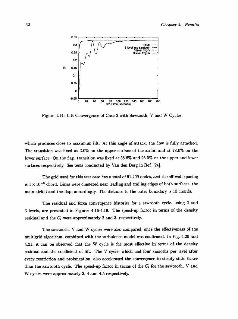
which produces close to maximum lift. At this angle of attack, the How is fully attached.

The transition was h e d at 3.0% on the upper surface of the airfoil and at 78.0% on the

lower surface. On the flap, transition was fixed at 58.8% and 95.0% on the upper and lower

surfaces respectively. See tests conducted by Van den Berg in Ref. 1241.

.J

i -1

- 1

The grid used for t his test case has a total of 91,409 nodes, and the off-wall spacing

is 1 x 10-~ chord. Lines were clustered near leading and trailing edges of both surfaces. the

main airfoil and the flap, accordingly. The distance to the outer boundary is 10 chords.

O 20 40 60 80 100 120 140 160 180 200 CPU IIme (seconds)

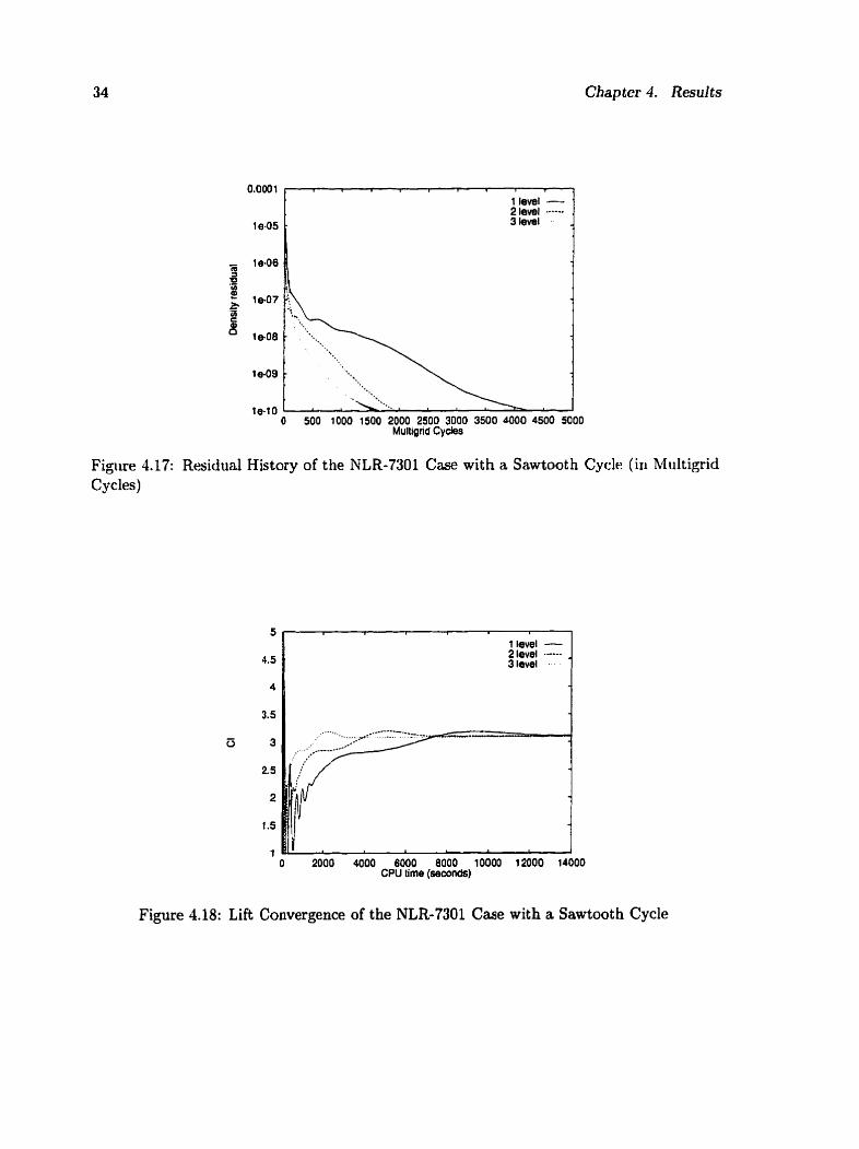
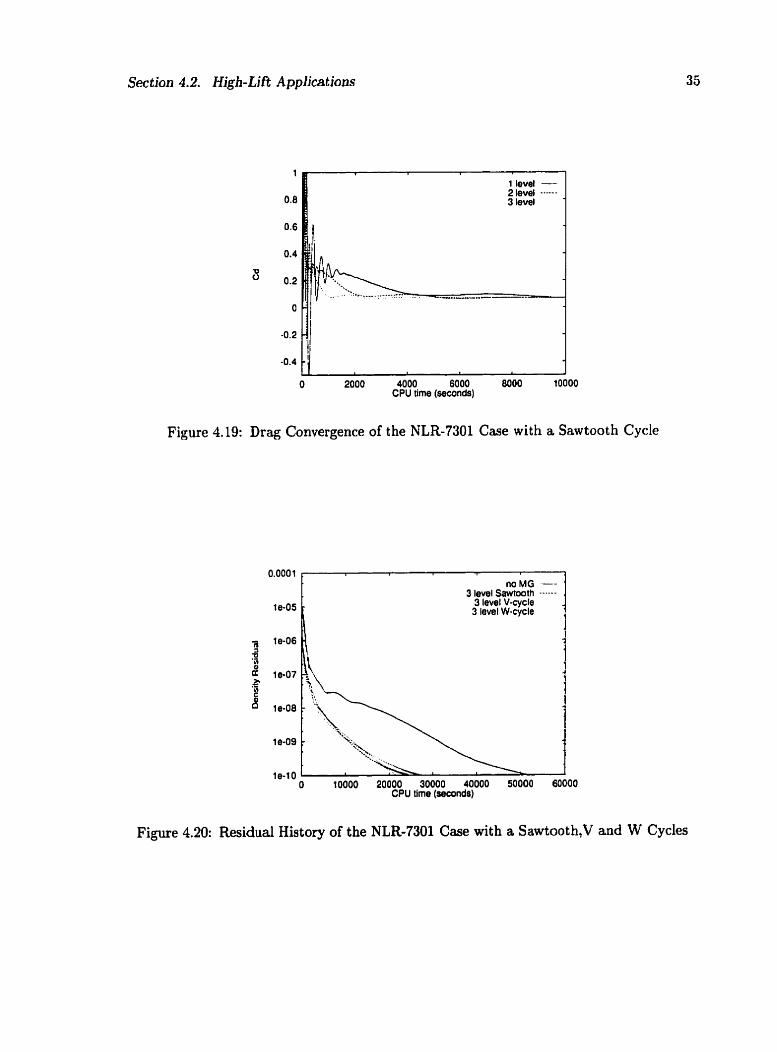
The residual and force convergence histories for a sawtooth cycle, using 2 and

3 levels, are presented in Figures 4.16-4.19. The speed-up factor in terms of the density

residual and the Cl were approximately 2 and 3, respectively.

The sawtooth, V and W cycles were also compared, once the effectiveness of the

multigrid algorithm, combined with the turbulence mode1 was confirmed. In Fig. 4.20 and

4.21: it c m be observed that the W cycle is the most effective in terms of the density

residual and the coefficient of lift. The V cycle, which had four smooths per level after

every restriction and prolongation, also accelerated the convergence to steady-state faster

than the sawtooth cycle. The speed-up factor in terms of the Cr for the sawtooth, V and

W cycles were approximately 3, 4 and 4.5 respectively.

Section 4.2. High- Lift Applications

Figure 4.15: Close-up of the NLR-7301 Grid

7

1 level - ' 2 level ------ , 3 level

1

O 10000 20000 30000 40000 50000 60000 CPU tirne (seconds)

Figure 1.16: Residual History of the NLR-7301 Case with a Sawtooth Cycle

Chapter 4. Results

0.0001

2 level a-----

19-05 3 level

O 500 1000 1500 2000 2500 3000 3500 4000 4500 5000 Multigrid Cycles

Figure 4.17: Residual History of the NLR-7301 Case with a Sawtooth Cycle (in Multigrid Cycles)

2 lévél ----- 3 level . .

O 2000 4000 6000 8000 10000 12000 14000 CPU lime (seconds)

Figure 4.18: Lift Convergence of the NLR-7301 Case with a Sawtooth Cycle

Section 4.2. High- Lift AppJica tions

1

0.8

0.6

0.4

0.2

O

-0.2

-0.4

O 2000 4000 6000 8000 10000 CPU time (seconds)

Figure 4.19: Drag Convergence of the NLR-7301 Case with a Sawtooth Cycle

3 levei Sawtwth ------ 3 level V-cycle 3 level W-cycle i

7

O 10000 20000 30000 40000 50000 60000 CPU time (seconds)

Figure 4.20: Residual History of the NLR-7301 Case with a Sawtooth,V and W Cycles

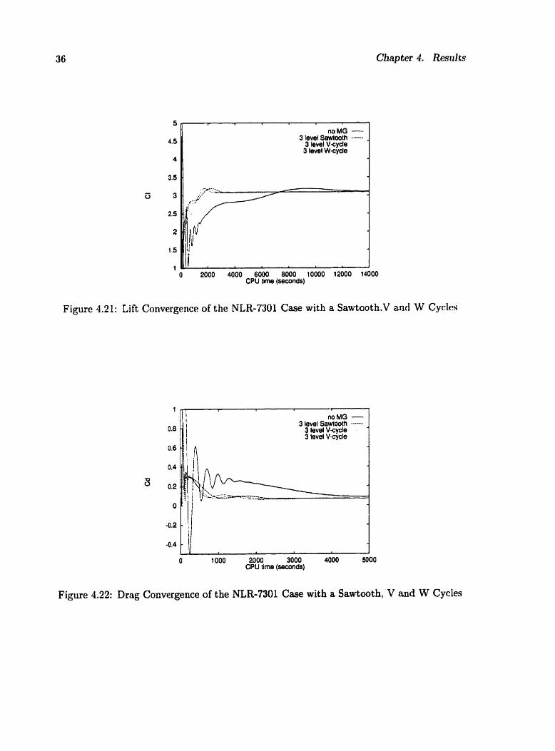
no MG - 3 levei Sawtoolh -a---

3 level V-cycle 3 level W-cycle

O 2000 4000 6000 8000 10000 12000 14000 CPU time (seconds)

Figure 4.21: Lift Convergence of the NLR-7301 Case with a Sawtooth.V and W Cycles

no MG - 3 level Sawtooth ------ .

3 level V-cycle 3 level V-cycle

Figure 4.22: Drag Convergence of the NLR-7301 Case with a Sawtooth, V and W Cycles

Section 4.2. High- Lift Applications

Table 4.1: Specified transition locations (percent of element chord)

4.2.2 Test Case 5: Case A-2 from the Advisory Report No. 303

a

4

The grid employed in this test case is a C-H-mesh configuration with a total of 46

blocks (see Fig. 4.23, formed by the removal of every other grid line of the fine grid). An

inner C-grid surrounds each airfoil element with thin blocks approximating the thickness of

the boundary layer. The off-wdl spacing is 1 x 10-~c, but increases locally to 1 x IO-% in

the coves of the slat and the flap. The outer bouiidary is located 10 chords away from the

airfoil. The grid has approximately 140,000 points. The Mach number and the Reynolds

number for this test case were 0.2 and 3.52 x 106 respectively. The angle of attack is 4.0

deg. Sransition points for the slat, main airfoil and flap are shown on the Table 4.1.

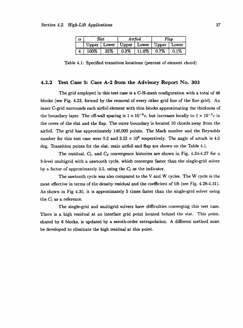
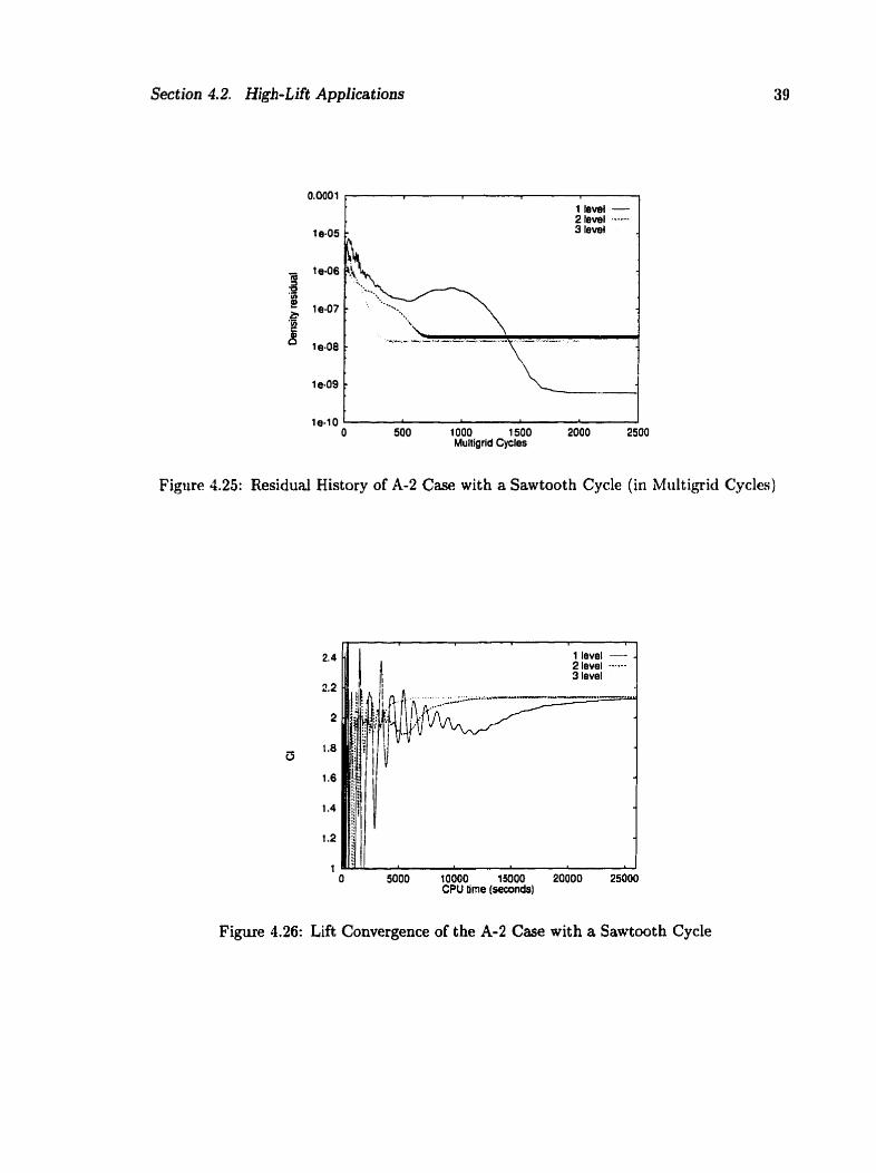
The residual, Ci, and Cd convergence histories are shown in Fig. 4.24-4.27 for a

3-level multigrid with a sawtooth cycle, which converges faster than the single-grid solver

by a factor of approximately 3.5. using the Ci as the indicator.

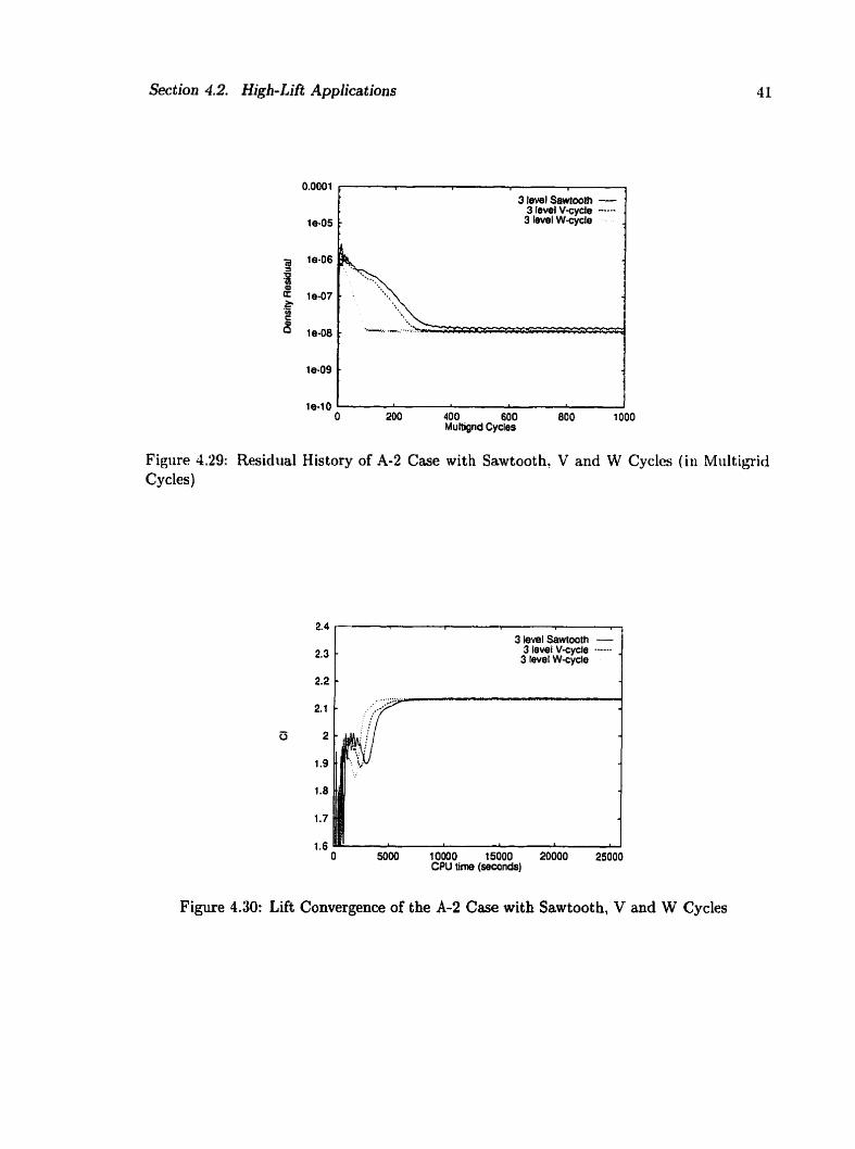
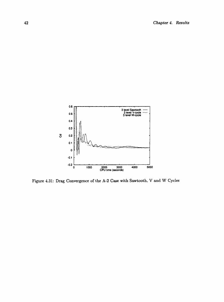
The sawtooth cycle was also compared to the V and W cycles. The W cycle is the

most effective in terms of the density residual and the coefficient of lift (see Fig. 4.28-4.31).

As shown in Fig 4.30, it is approximately 5 times faster than the single-grid solver using

the Cl as a referexice.

The single-grid and multigrid solvers have difficulties converging this test case.

There is a high residual at an interface grid point located behind the slat. This point,

shared by 6 blocks, is updated by a zeroth-order extrapolation. A different rnethod Inust

be developed to eliminate the high residud at this point.

A irfoil Slat

Upper 0.3%

Upper 100%

Flap Lower 11.0%

Lower

25% Upper 0.7%

Lower 0.1%

Chapter 4. Results

Figure 4.23: Close-up of the A-2 Grid

1 1

1 level - ' 2 level -- 3 Ievel . - .

, 1 5000 10000 15000 20000 25000 30000

CPU lime (seconds)

Figure 4.24: Residual History of A-2 Case with a Sawtooth Cycle

Section 4.2. High-Lift Applications

Figure 4.25: Residual History of A-2 Case with a Sawtooth Cycle (in Miiltigrid Cycles)

2.4

2.2

2

1.8 B

1.6

1.4

1.2

1 O 5000 10000 1NOO 20000 25000

CPU time (seconds)

Figure 4.26: Lift Convergence of the A-2 Case with a Sawtooth Cycle

Chapter 4. Results

Figure

0.6

0.5

0.4

0.3

0.2

0.1

O

-0.1

70.2 O 5000 10000 15000 20000

CPU time (seconds)

Drag Convergence of the A-2 Case with a Sawtoot

3 level Sawtooth - 3 level V-cycie ----

3 kvel W-cyde .

Cycle

19-10 O 2000 4000 6000 8000 10000 12000 14000 16OOOl8OOO2OOOO

CPU time (seconds)

Figure 4.28: Residual History of A-2 Case with Sawtooth, V and W Cycles

Section 4.2. Hi&- Lift Applications

I I

3 level Sawtoolh - ' 3 tevel V-cycle ------ , 3 level W-cycle

7

O 200 400 600 800 1 O00 Multignd Cycles

Figure 4.29: Residual History of A-2 Case with Sawtooth, V and W Cycles ( in Miiltigrid CycIes)

b. 7

3 level Sawtoath - 2.3 / 3 levet V-cycle ------

3 tevel W-cycle i

O 5000 10000 t5000 20000 25000 CPU tirne (seconds)

Figure 4.30: LiEt Convergence of the A-2 Case with Sawtooth, V and W Cycles

F 3 level Sawtwth -

3 level V-cycle ------ . 3 level W-cycle

C . : 1 . . 4 . . . , . . . . , ,

, . , ,

-0.2 1 I

O 1 O00 2000. 3000 4000 5000 CPU tirne (seconds)

Figure 4.31: Drag Convergence of the A-2 Case with Sawtooth, V and W Cycles

Chapter 5

Conclusions and Recommendat ions

An efficient global-multigrid algorithm has been added to the TORNADO rriiilti-

block solver. The multiblock-multigrid solver is as efficient as the single-block miiltigrid of

the SC1 solver. In the high-lift cases. the best niultigrid cycle is the W cycle. foIlowed by

the V and sawtooth cycles. Three-level multigrid proved to be most effective at the removal

of the error. With the addition of multigrid, TORNADO converges to steady state three

to six times faster thari previously.

It would be worth studying the effect on convergence of not applying multigrid to

some of the blocks of the grid. In some cases, the error can be easily rentoved from some

blocks and applying the multigrid cycle is not necessary. It woiild be important to develop

a schcme to deterinine if multigrid should not be applied to some blocks of the grid. This

would make the algorithm more effective and no unnecessary effort would be devoted to

blocks wbere low-frequency errors are not present.

References

111 Beam, R.M. and Warming, R.F., LLAn Implicit FiniteDifference Algorithm for H y p w

bolic Systems in Conservation Law Form," .J. Comp. Phys., Vol. 22, 1976, pp. 87-110.

[2] Steger, J.L., 4mplicit Finite Differeiice Simulation of Flow about Arbitrary Geometries

with Application to Airfoils," AIA A paper, 1977, pp. 77-665.

[3] Pulliam, T. H., "Efficient Solution Methods for the Navier-Stokes Equations," Lect tire

Notes For The Von Karman Institute For Fluid Dynarnics Lecture Series: Numerzcal

Techniques F o r Viscous Flow Computation 111 lhrbomachinery Bladings, Jan. 1986.

[4] Jameson, A., "Solution of the Euler Equations for Two Dimensional Tkansonic Flow by

a Multigrid Method," Applied Mathenaatics and Computation, Vol. 13? 1983, pp. 327-

356.

[5] Jameson, A., "Multigrid Solut ions of the Euler Equations using Implicit Schemes,"

AIAA journal, Vol. 24, No. 11, 1986, pp. 1737-1743.

[6] Martinelli, L. and Jameson, A. and Grasso, F., "A Multigrid Metbod for the Navier-

Stokes Equations," AIAA paper 86-0208, 1986.

[7] Jameson, A. and Schmidt, W. and Turkel, E., "Numerical Solutions of the Euler Equa-

tions by Finite Volume Methods Using Runge-Kutta Time-Stepping," AIAA Paper

81-1259, June 1981.

[8] Caughey, D .A., "Diagonal Implicit Multigrid Algorit hm for the Euler Equations,"

AIAA Journal, Vol. 26, No. 7, July 1988.

[9] Yadlin, Y. and Caughey, D.A., "Block Multigrid Implicit Solution of the Euler Equa-

tions of Compressible Fluid Flow," AIAA Journal, Vol. 29, No. 0275, May 1991.

Referen ces 45

[IO] Wang, L. and Caughey, D.A., 'bMultiblock/Multigrid Euler Method to Simulate 2D

and 3D Compressible Flow," AIAA Journal, Vol. 32, No. 3, March 1993.

[Il] Chisholm, T., Multigrid Acceleration of an Approxàmately-Factored Algorithm for

Steady Aerodynarnic Flows, Master's thesis, University of Toronto, Jan. 1997.

[12] Jespersen, D.C., Pulliam, T. and Buning, P., "Recent Enhancements to OVERFLOW ," AIAA paper 97-0644, January 1997.

[13] Thompson, J.F., "A Composite Grid Generation Code for General 3-D Regions -the

EAGLE code," AIAA Journal, Vol. 26, No. 3, 1988.

[14] Nelson, T. E., Numerical Solution of the Navier-Stokes Equations for High-Làft Airfoil

Configurations, Ph.D. thesis. University of Toronto, May 1994.

[15] Godin. P. and Zingg, D.W. and Nelson, T.E., "High-Lift Aerodynamic Computations

with One- and Two-Equation Turbulence Models," A IAA .Journal? Vol. 35. No. 2. Fcb.

1997, pp. 237-243.

[16] Nelson. T. E. and Zingg, D. W. and Johnston. G. W., "Compressible Navier-Stokes

Computations of Multielement Airfoil Flows Using Multiblock Grids.?' A I A A ,Jounlal.

Vol. 32, No. 3, March 1994.

117) Fejtek, I., "Summary of Code Validation Results for a Multiple Element Airfoil Test

Case," AIAA paper 97-1932, June 1997.

[18] Spalart, P. R. and Allmaras, S. R., "A One-Equation Turbulence Mode1 for Aerody-

namic Flows," AIAA Paper 92-0439, January 1992.

[19] Jespersen, D.C., *Multigrid Met hods for Partial Differential Equations," Studies in

Numerical AnalysZs, Vol. 24, 1985, pp. 278-318.

[20] Wesseling, P., "Introduction to Multigrid Methods," ICASE Report No. 95-1 1, Feb.

1995.

[21] Maksymiuk, C.M.? Swanson, R.C. and Pulliam T.H., "A Comparison of Two Cen-

tral Difference Schemes for Solving the Navier-S t okes Equat ions," NASA Tech. Memo

102815, 1990.

46 References

[22] Wilkinson, A.R. and Zingg, D.W., 'TORNADO User's Guide," Nov. 1993.

[23] De Rango, S. and Zingg, D.W., "SC1 User's Guide," Jan. 1997.

[21] Van den Berg, B., "Boundary Layer Measurements on a Two-Dimensional Wing with

Flap," National Aerospace Lab., NLR TR 79009, Jan 1979.

Appendix A

Mult igrid Pseudo-codes

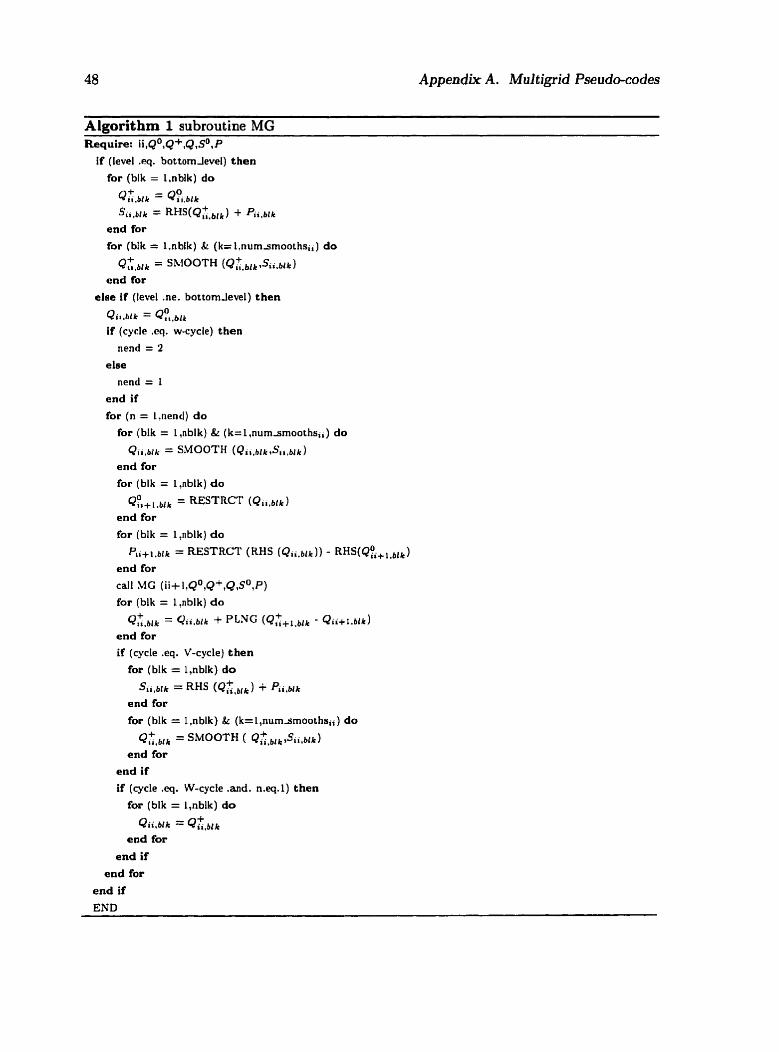
Pseudo-code is presented for a multiblodc solver wi t h global rnultigrid. This niulti-

grid subroutine, called MG. can be used for any of the multigrid cycles: Sawtoot h, V cycle.

and W cycle. Subscripts denote the level and block under consideration, wherenr siiper-

scripts indicate the stage. "blk" and "nblk" represent the specific block and the total

number of blocks in the grid repectively. "num~rnooths" indicates the number of iterations

per multigrid level.

48 Appendix A. Mul tigrid Pseudo-codes

Alnorithm 1 subroutine MG Require: ~ ~ , Q O , Q + ,Q,sO,p

if (Ievel .cq. bottomlevel) then

for (blk = 1,nblk) do

~ ~ , b l k = Q?t,blk

Sii,blk = RHS(Q;&~) Pii,blk

end for

for (blk = l,nblk) & (k=l,numsmoothsii) do

Q:,blk = SbIOOTH (Q:,blk ,sii.blk ) end for

else if (level .ne. bottom-level) then

Qit.61~ = QI)l,blk

if (cycle .eq. w-cycle) then

nend = 2

nend = 1

end if for (n = 1,nend) do

for (blk = 1,nblk) & (k=l,numsmoothsi,) do

Qii.b~k = SMOOTH (Qi,.h~ktSti.b~k)

end for

if (cycle .eq. V-cycle) then

for (blk = 1,nblk) d o

Sri.blk = RHS ( Q : , ~ , ~ ) + Pii.blk

end for

end if

if (cycle .eq. W-cycle .and. n.eq.1) then for (blk = 1,nblk) do

Qii,blk = Q : , ~ ~ ~ end for

end if

end for

end if END