an evaluation of multigrid acceleration for the simulation ... · pdf filethe multigrid method...

Copyright © 2015 Tech Science Press CMES, vol.106, no.3, pp.203-228, 2015

An Evaluation of Multigrid Acceleration for theSimulation of an Edge FLame in a Mixing Layer

M. Wasserman1,2, Y. Mor-Yossef1,2 and J.B. Greenberg1

Abstract: A test problem of a laminar edge flame formed in the mixing layer oftwo initially separated streams of fuel and oxidant is employed to evaluate the per-formance of multigrid acceleration of the iterative solution of the central differencefinite difference scheme approximating the governing energy and species mass frac-tion conservation equations. The multigrid method was found to be extremely effi-cient and significantly improved the iterative convergence relative to that of a singlegrid method. For low to moderate chemical Damkohler numbers, acceleration fac-tors of up to six (6!) times were recorded in the computational time required toobtain iterative convergence with the multigrid method, over that required with thesingle-grid method to obtain the same level of convergence. Moreover, monotonicconvergence was obtained with the multigrid method in cases where the conver-gence of the single-grid method stalled. However, for large chemical Damkohlernumbers of more than a thousand (i.e. very small characteristic chemical reac-tion times) and three levels of grid refinement the advantage of application of themultigrid method was seriously degraded due to the necessity to dampen errorsstemming from the highly nonlinear chemical source terms on coarse grid levels ofthe multigrid hierarchy.

Keywords: Multigrid, finite differences, edge flames.

1 Introduction

In a recent PhD thesis Wasserman (2014) presented a comprehensive multi-gridbased numerical strategy for RANS (Reynolds-averaged Navier-Stokes simula-tions) of steady state turbulent reacting flows. The study was motivated by theconstantly growing complexity of turbulent combustion CFD simulations, impos-ing severe demands on computational resources. Such demands often render thesimulation of practical, supersonic reacting flows over complex geometries unaf-

1 Faculty of Aerospace Engineering, Technion – Israel Institute of Technology., Haifa, Israel 32000.2 Israeli CFD Center, Caesarea Industrial Park, Israel 38900.

204 Copyright © 2015 Tech Science Press CMES, vol.106, no.3, pp.203-228, 2015

fordable. As standard numerical methods are inefficient in solving the highly stiff,reacting (RANS) equations which govern turbulent combustion, there exists a needfor methods that accelerate the iterative convergence to a steady-state.

Perhaps the foremost problem associated with numerical solution of the equationsgoverning reacting flow is the strong numerical stiffness. A given set of differen-tial equations is considered numerically stiff when the physical processes describedby it (e.g., convection, diffusion and chemical reaction) develop on very differenttime scales, or equivalently, when the corresponding eigenvalues of the discretized,algebraic equation set vary greatly [Gear (1971)]. Numerical stiffness may signif-icantly limit convergence rates of standard iterative methods, and results in lack ofrobustness of numerical simulations, unless properly treated [Lomax, Pulliam andZingg (2001]. The numerical stiffness of the reacting RANS equation set may beattributed to several factors. In high Reynolds number applications prominent inaeronautical engineering, extremely dense meshing is employed near solid walls toaccurately resolve boundary layers, leading to highly stretched cells. As a result,the characteristic time scales of convection and diffusion processes may differ con-siderably, and the resulting eigenvalues of the system may be spread over a widerange of values. This effect may be noted even in some non-reacting, laminar sim-ulations. Moreover, finite-rate chemistry and turbulence modeling introduce severenumerical stiffness owing to the nature of source terms appearing in both models.The source terms which represent the production and dissipation of turbulence, andthe transformation of species due to chemical reactions, are often strongly nonlinearand contain time scales that greatly differ from those of the convective and diffusiveterms. The turbulence dissipation time scale may vary by many orders of magni-tude across a turbulent boundary layer, and can be vastly different from the othertime scales (e.g. molecular diffusion and wave propagation). In addition, chem-ical kinetics, especially for combustion, is characterized by widely disparate timescales related to formation and depletion of different species. In high-speed com-bustion of hydrogen with air, for instance, the characteristic time scales of hydroxyl(OH) formation are extremely short (10−8 sec.), while the characteristic time scalesof water vapor formation are relatively long (10−2 sec.) [Bussing (1985)]. It isthis time-scale disparity that leads to numerical stiffness. Any numerical approachaimed at solving the RANS equations coupled with turbulence and/or chemistrymodel equations should be able to reflect all the different time scales present in theflow to ensure stability and accuracy. To comply with this requirement, the allowedtime-step is limited by the rate of the fastest chemical reaction.

Geometric multigrid (MG) methods are amongst the fastest numerical accelerationtechniques known today. Basically, MG methods accelerate convergence rates ofnumerical schemes by using a hierarchy of grids, based on the notion that some nu-

An Evaluation of Multigrid Acceleration 205

merical error modes are more efficiently treated on a coarse grid than on a fine grid.However, a coarse grid may only be used in conjunction with a finer one, requir-ing proper data transfer between consecutive grids. MG methods rely on two basicprinciples: Smoothing and Coarse Grid Correction (CGC). First, standard iterativemethods (e.g., Gauss-Seidel) with good smoothing (that is, elimination of high spa-tial frequency modes) properties are used to treat non-smooth errors in the solution.Pre-smoothing is required because only a smooth error is represented well on bothfine and coarse grids, while non-smooth errors exhibit aliasing on coarse grids, sig-nificantly reducing the efficiency of coarse grid corrections [Yavneh (2006)]. Aftera smooth error is obtained on the finest grid where a solution is sought, relaxationcontinues on coarser grids which are achieved by eliminating every other grid linein each coordinate direction (on structured grids). A coarse grid relaxation is sub-stantially cheaper (up to four times in 2D) than its fine grid counterpart, and isalso more efficient in eliminating errors which are relatively smooth on a finer grid.Thus, efficiency can be increased by transferring (restricting) some of the fine griditerations required for convergence, to a coarser grid, and interpolating (prolongat-ing) the results, that is, applying a coarse grid correction, to advance the solutionon the finest grid. MG methods are widely popular, and well defined in a mathe-matical sense [Briggs and McCormick (2000), Trottenberg, Oosterlee, and Schuller(2001)]. Beginning with the pioneering work of Brandt (1977), who first presentedan unprecedented efficiency of MG methods for elliptic boundary-value problems,and the Full Approximation Storage (FAS) MG method for nonlinear equations,many researchers have been using this class of methods in a wide variety of fieldssuch as CFD, image processing and medical science.

However, while for simple model problems based on elliptic PDEs, optimal text-book multigrid efficiency (TME) [Trottenberg, Oosterlee, and Schuller (2001)] wasdemonstrated more than three decades ago [Brandt (1977)], modern MG methodsfor mixed-nature, non-linear equations such as the RANS equations are still farfrom optimal [Brandt (1998)]. For instance, MG methods for the Navier-Stokesequations are known to suffer from convergence difficulties in high Reynolds vis-cous flows. The successful incorporation of turbulence and species mass transportequations in the multigrid framework still remains a major barrier to demonstrat-ing an optimally efficient MG method for the reactive RANS equations [[Brandt(1998)]]. Indeed, finite-rate chemistry currently poses a significant challenge forstandard multigrid methods. In the case of a full coarsening multigrid strategy,coarse grid variables are linearly calculated from corresponding fine grid values.Recalculation of strongly non-linear chemical kinetics source terms on coarse gridsbased on linearly averaged variables may cause large differences compared to fine-grid values. In most cases, the consequence is divergence of classic multigrid


schemes [Gerlinger, Mobus and Bruggemann (2001)]. Moreover, since chemicalreaction zones are usually very small, coarse grid level solutions may not suffi-ciently resemble those obtained on the fine grid levels [Edwards and Royt (1998)].For example, if fuel and oxidizer are separated on a grid with fine resolution, thisis not necessarily the case in an equivalent coarse grid level where mixing (com-bustion) may occur due to insufficient spatial resolution. To overcome these diffi-culties, extensive stabilization is employed by the few researchers who publishedresults of attempts at applying multigrid to chemically reacting flows.

Sheffer, Jameson and Martinelli (1998) only managed to achieve convergence usinga two-level, explicit multigrid simulation of detonation waves. Slomski, Andersonand Gorski (1990) simulated reacting flows using standard multigrid procedures,but demonstrated acceleration only for low supersonic flows with reduced chem-ical kinetics models. Edwards (1996) applied multigrid to hypersonic chemicallyreacting flows and hydrogen combustion [Edwards and Royt (1998)], but had toemploy global damping of the restricted residuals and lowered CFL numbers oncoarse grids to stabilize the solution. To avoid global damping, a local dampingof the restricted residual in regions of high chemical activity was suggested byGerlinger, Mobus and Bruggemann [(2001)] and Gerlinger (2005), allowing forharvesting the full potential of multigrid in regions without combustion. Kim, Kimand Rho (2001) employed a damped prolongation procedure based on the ratio oflocal pressure values from the coarse and fine grids to damp coarse-grid correctionsin the vicinity of shock-waves. Bellucci and Bruno (2001) were able to devise afour-level multigrid method for three-dimensional incompressible flows with com-bustion. However, they applied Laplacian smoothing of coarse-grid corrections andpresented convergence rates only for non-reacting cases. Another drawback of allapproaches mentioned is the dependence on user-supplied parameters which sig-nificantly lowers the robustness of multigrid reacting flow simulations [Gerlinger(2005)].

To overcome the aforementioned difficulties Wasserman (2014) proposed using theunconditionally positive-convergent (UPC) time integration implicit scheme [Mor-Yossef and Levy (2006, 2007, 2009) and Wasserman, Mor-Yossef, Yavneh andGreenberg (2010)] originally developed for turbulence model equations, and suc-cessfully extended its use with chemical kinetics models, in a fully-coupled multi-grid (FC-MG) framework.

To tackle the degraded performance of multigrid methods for chemically react-ing flows, two major modifications were introduced with respect to the basic FullApproximation Storage (FAS) multigrid method. First, a novel prolongation oper-ator based on logarithmic variables was proposed to avoid loss of positivity due tocoarse grid corrections. The use of a positivity-preserving prolongation operator,


together with the extended UPC implicit scheme, ensure unconditional positivity ofturbulence quantities and species mass fractions throughout the multigrid simula-tion. Secondly, in order to improve the coarse grid correction obtained in localizedregions of high chemical activity, a modified defect correction procedure was de-vised, and successfully applied for the first time to solve turbulent, combustingflows. The proposed modifications to the standard multigrid algorithm created awell-rounded robust numerical method that provides accelerated convergence withrespect to an equivalent single-grid-based method, and unconditionally preservesthe positivity of model equation variables. The resulting MG method is suitable forrobust simulations of a wide range of flows thanks to being nearly completely freeof artificial stabilization techniques.

Numerical simulation of various turbulent and reacting flows showed that the pro-posed MG method increases the efficiency by a factor of up to eight (8!) timeswith respect to an equivalent single-grid method, and by two times with respectto an artificially-stabilized MG method. Moreover, the method has proven to bemore stable than an equivalent SG-based method, allowing the use of higher CFLnumbers, and rapid convergence in cases where the SG-based method failed to con-verge.

The majority of examples of reacting flow to which MG was applied involvedpremixed reacting flows and employed various degrees of chemical complexityin terms of the actual details of the participating elementary chemical reactions.It is well-known that the nature of non-premixed combustion is rather different[Williams (1985) and Law (2006)] and little attention has been paid to accelerationof numerical schemes for dealing with non-premixed reacting flows.

In the present paper we present a first evaluation study of the application of multi-grid acceleration for the simulation of an edge flame in a laminar mixing layer.The main purpose of the investigation is to provide initial insight into the relevanceand/or scope of multigrid acceleration in this context without the additional com-plexities of turbulence.

2 Mathematical Model and Assumptions

We consider two parallel streams of equal (constant) laminar velocity, one of gaseousfuel and the other of oxygen. The two streams are separated upstream by a semi-infinite flat plate (see Figure 1). The temperature of the plate is assumed constantand equal to the upstream temperature of the two streams. Downstream of the plate,under appropriate operating conditions, chemical reaction occurs. It will be takento be represented by a single global reaction step of the form:

Fuel + ν Oxidizer→ (1+ν) Products + thermal energy, where ν is the stoichiomet-


ric coefficient.

Figure 1: Configuration for study of an edge flame: the broken line.

Downstream of the tip of the plate diffusive mixing of the fuel and oxygen occursand a mixing layer is formed. What is known as an edge flame arises, locatedsomewhere downstream of the plate’s tip. We refer to this edge flame as the rootof the diffusion flame that is attached to and trails downstream from it. Whenthere is only moderate premixing of reactants the edge flame is characterized by areaction kernel with a volumetric reaction rate much greater than that of the trailingdiffusion flame. In Fig. 1 typical reaction rate contours are shown. Because ofthe premixing zone before the onset of reaction the entire structure of the flame isthat of a partially premixed flame (at the root) followed by a trailing downstreamdiffusion flame. This configuration was examined numerically by Kurdyumov andMatalon (2004) with particular emphasis on the dynamics of such flames. In thecurrent work we concentrate on obtaining steady state solutions using multigridacceleration.

Further reasonable assumptions which are adopted are that the density of the gasmixture, ρ , the thermal diffusivity, Dth, the specific heat capacity at constant pres-sure, Cp, and the molecular diffusion coefficients of fuel and oxidant, DF , DO,respectively, are constant. Under these and the aforementioned assumptions weobtain the following non-dimensional thermal-diffusional formulation of the gov-erning equations:

∂YF

∂x=

1LeF

∇2YF −ω (1)

∂YO

∂x=

1LeO

∇2YO−φω (2)


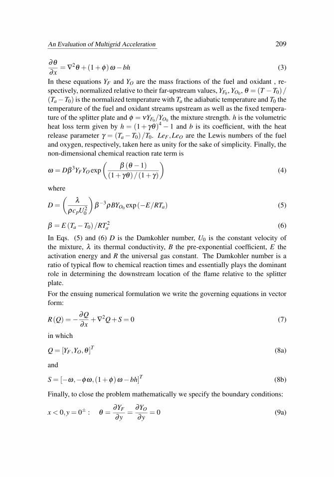
∂θ

∂x= ∇

2θ +(1+φ)ω−bh (3)

In these equations YF and YO are the mass fractions of the fuel and oxidant , re-spectively, normalized relative to their far-upstream values, YF0 , YO0 , θ = (T −T0)/(Ta−T0) is the normalized temperature with Ta the adiabatic temperature and T0 thetemperature of the fuel and oxidant streams upstream as well as the fixed tempera-ture of the splitter plate and φ = νYF0/YO0 the mixture strength. h is the volumetricheat loss term given by h = (1+ γθ)4− 1 and b is its coefficient, with the heatrelease parameter γ = (Ta−T0)/T0. LeF ,LeO are the Lewis numbers of the fueland oxygen, respectively, taken here as unity for the sake of simplicity. Finally, thenon-dimensional chemical reaction rate term is

ω = Dβ3YFYO exp

(β (θ −1)

(1+ γθ)/(1+ γ)

)(4)

where

D =

(λ

ρcpU20

)β−3

ρBYO0 exp(−E/RTa) (5)

β = E (Ta−T0)/RT 2a (6)

In Eqs. (5) and (6) D is the Damkohler number, U0 is the constant velocity ofthe mixture, λ its thermal conductivity, B the pre-exponential coefficient, E theactivation energy and R the universal gas constant. The Damkohler number is aratio of typical flow to chemical reaction times and essentially plays the dominantrole in determining the downstream location of the flame relative to the splitterplate.

For the ensuing numerical formulation we write the governing equations in vectorform:

R(Q) =−∂Q∂x

+∇2Q+S = 0 (7)

in which

Q = [YF ,YO,θ ]T (8a)

and

S = [−ω,−φω,(1+φ)ω−bh]T (8b)

Finally, to close the problem mathematically we specify the boundary conditions:

x < 0,y = 0± : θ =∂YF

∂y=

∂YO

∂y= 0 (9a)


{(x→−∞,y > 0)∪ (all x,y→+∞)} : θ = 0,YF = 1,YO = 0 (9b)

{(x→−∞,y < 0)∪ (all x,y→−∞)} : θ = 0,YF = 0,YO = 1 (9c)

x→ ∞ :∂θ

∂x=

∂YF

∂x=

∂YO

∂x= 0 (9d)

The first boundary conditions represent conditions on the splitter plate which is atfixed normalized temperature (i.e. zero) and is impervious to mass transfer. Thesecond conditions relate to conditions far upstream above the splitter plate as wellas at the upper boundary of the domain. Similarly, the third conditions give condi-tions far upstream below the plate as well as at the lower boundary of the domain.Finally, the last conditions state that far downstream no changes occur in the massfractions and the temperature.

The finite solution domain and the aforementioned boundary conditions are shownschematically in Fig. 2.

Figure 2: Schematic of solution domain and boundary conditions.

3 The Numerical Approach

Finite differences are utilized for discretization of the governing equations and therelevant boundary conditions. Using subscripts i, j, for the x and y directions,respectively and ∆x, ∆y for increments in those directions we have:

xi = x1 +(i−1) ·∆x , i = 1..Ny j = y1 +( j−1) ·∆y , j = 1..M

(10)


where we take x1 = −5, xN = 15, y1 = −15, yM = 15 so that conditions at the farboundaries are well represented. N and M were chosen to ensure that the tip of thesplitter plate, (x,y) = (0,0), is a mesh point. In this work the x and y incrementswere both taken equal to h.

The governing equations were discretized using central differences for the spatialderivatives so that for non-boundary points

R(Qi, j) =−Qi+1−Qi−1

2∆x+

(Qi+1−2Qi +Qi−1

∆x2 +Q j+1−2Q j +Q j−1

∆y2

)+Si = 0

∀ i = 2..N−1, j =(

1..M2−1,

M2+2..M−1

)(11)

with local accuracy of O(∆x2,∆y2

).

The boundary conditions become:

At the upper and lower boundaries:

Q(i = 1..N, j = 1) = [0,1,0]T

Q(i = 1..N, j = M) = [1,0,0]T

On the lower and upper sides of the splitter plate second order backward and for-ward differences are used, respectively, for the mass fraction derivatives:

Q(i = 1..Nw, j = M/2)1,2 =

[−Q(i = 1..Nw, j = M/2−2)/3+4Q(i = 1..Nw, j = M/2−1)/3

]

Q(i = 1..Nw, j = M/2+1)1,2 =

[−Q(i = 1..Nw, j = M/2+3)/3+4Q(i = 1..Nw, j = M/2+2)/3

]where the subscripts "1,2" relate to the fuel and oxidant mass fractions, respectively,and "w" to the value on the wall (plate).

For the temperature along the plate:

Q(i = 1..Nw, j = M/2+1)3 = 0

In the far field:

Q(i = N, j = 2..M−1)1,2,3 =

−Q(i = N−2, j)/3+4Q(i = N−1, j)/3

The subscript "3" refers to the normalized temperature which is the third componentof the vector Q.


At the left hand (entrance) boundary below the splitter plate

Q(i = 1, j = 2..M/2)1,2,3 = [0,1,0]T

whereas above it

Q(i = 1, j = 2..M/2+1..M−1)1,2,3 = [1,0,0]T .

4 The Numerical Solution

4.1 Basic solution method

The point Jacobi method is employed for solving the set of nonlinear algebraicequations that replace the original governing equations. The advantages of thismethod lie in its ability to be readily parallelized for large problems and its effi-cient error smoothing property which is essential for effective application of themultigrid method. The point Jacobi scheme relevant to the current problem at anypoint in the solution domain and for iteration number n is

Qn+1i, j =

(−Qn

i+1, j−Qni−1, j

2∆x +Qn

i+1, j+Qni−1, j

∆x2 +Qn

i, j+1+Qni, j−1

∆y2 +Sni, j−

(∂Si, j∂Qi, j

)nQn

i, j

)(

2∆x2 +

2∆y2 −

(∂Si, j∂Qi, j

)n) (12)

Note that the source term has been linearized about the previous iteration.

The analytical Jacobian is given by

∂Si, j

∂Qi, j=

−ω/YF

−ω/YO

− ∂ω

∂θ

−φω

YF−φ

ω

YO−φ

∂ω

∂θ

(1+φ) ω

YF(1+φ) ω

YO

(1+φ) ∂ω

∂θ

−4b(1+ γθ)3γ

i, j

where

∂ω

∂θ=

ωβ (1+ γ)2

(1+ γθ)2 > 0

To allow for larger time-steps, an implicit solution is sought, requiring that alleigenvalues, λi of the Jacobian, ∂Si, j/∂Qi, j, satisfy Re(λi)< 0.

For this purpose, use is made of an approximate source term Jacobian of the form

∂Si, j

∂Qi, j=

−ω/YF 0 00 −φ

ω

YO0

0 0 −4b(1+ γθ)3γ

i, j

(13)


For convenience the actual Jacobian was diagonalized since when convergence to asteady state is attained this term becomes irrelevant. Diagonalization contributes tocomputational efficiency as it preserves a scalar partitioning at each iteration In ad-dition, the positive term (1+φ)∂ω

/∂θ (stemming from the temperature Jacobian

terms) was omitted because of stability considerations.

For the purpose of stability and error smoothing under-relaxation was also utilized:

Qn+1i, j = w

(Qn+1

i, j

)Jacobi

+(1−w)Qni, j (14)

with a value of 0.9 assigned to the relaxation parameter w, providing optimal per-formance for most of the cases studied here.

The initial guess was based on an analytical solution of the problem which canbe deduced when the Damkohler number tends to infinity. For further details theinterested reader is referred to Kurdyumov and Matalon (2004)

The convergence of the iterative procedure was checked using the following crite-rion

En =

√N−1∑

i=2

M−1∑j=2

(Rn

i, j

)2

(N−2) · (M−2)< 10−6 (15)

4.2 Multigrid application

Because of the strongly nonlinear nature of the problem FAS multigrid was applied.With this method the discrete problem is solved on a hierarchy of meshes of differ-ent levels of refinement obtained by deleting every second point in each directionof the basic mesh (h) as sketched in Fig. 3.

In order to obtain significant iterative convergence it was necessary to employ atleast three levels of mesh refinement.

The stages of application of the multigrid method are enumerated here:

(1) Fine-grid pre-relaxation:Rh(Qh)= dh.

A number of point-Jacobi iterations with under-relaxation are performed in orderto smooth the error (dh).

(2) Restriction to a coarser grid: RH(I H

h Qh)−RH

(I H

h Q̄h)=−I H

h

(dh)

in which I Hh is the coarsening operator and Q̄h is the approximation to Qh. In

order to obtain a significant contribution to the solution from the finer grid the errorfrom the finer grid is transferred to the coarser grid using a coarse grid operator


Figure 3: A coarse mesh obtained by deleting every second point of the basic mesh.

comprised of weighted neighboring values from the fine grid as per the following:

d2h (x,y) = I2hh dh (x,y) =

(116

)4dh (x,y)+2dh (x+h,y)+2dh (x−h,y)+2dh (x,y+h)+2dh (x,y−h)+dh (x+h,y+h)+dh (x+h,y−h)+dh (x−h,y+h)+dh (x−h,y−h)

(16)

The error that is transferred acts as a source term that “drives” the solution on thecoarser grid thereby contributing to decreasing the error on the finer grid.

In some cases, specifically at the early stages of the numerical simulation, the fine-grid residual is very large, and not necessarily smooth, so that when it is transferredto the coarse-grid, it may result in divergence due to aliasing and due to the highlynon-linear nature of chemical source terms. To avoid this, a damped restrictionoperator is introduced, as follows:

RH(I H

h Qh)−RH

(I H

h Q̄h)=−I H

h

(α ·dh

)where α is a positive damping factor, taken to be smaller than one. In this worktwo possible methods of damping the error transferred to the coarse grid, dh, wereconsidered:

(a) local damping of the transferred error only in regions where significant chemicalreaction occurred, via the following formula [Gerlinger, Mobus and Bruggemann


(2001)]:

G(x,y) =max [ωh (x,y) ,ωh (x±h,y±h)]

max(ωh)

α (x,y) = max[0, 1−0.4 ·G(x,y)0.3

] (17)

and (b) fixed global reduction of the transferred error.

The different strategies for determining α are compared in section 5.

(3) Coarse-grid relaxations: RH(Q̄H)= RH

(I H

h Q̄h)−I H

h

(α ·dh

)+dH .

A number of iterations of the point Jacobi method with under-relaxation are carriedout to obtain a better approximation, Q̄H , which satisfies the equation that includesthe error term from the fine grid on the coarse grid. After carrying out these iter-ations one can return to the finer grid or apply the algorithm recursively (i.e. totransfer to an even coarser grid in order to obtain an even better solution to theequation on the coarser grid).

(4) Coarse grid correction: Q̄h = Q̄h +I hH(Q̄H −I H

h Q̄h).

The correction from the coarser grid is transferred to the finer grid where it is usedto update the current approximation to the solution. The interpolation operator, Ih

H ,used to transfer the correction to the finer grid (prolongation) is bi-linear interpola-tion, as illustrated in Fig. 4.

The afore-described multigrid stages were applied cyclically, in a V-cycle, as sketchedin Fig. 5. Since cycling replaces single grid iteration additional computation isrequired. In order to be able to correctly compare between achievement of con-vergence using multigrid and via a single grid we will use work units (WU). Eachwork unit is equivalent to the computer time necessary to carry out a single iterationon the finest grid in the hierarchy.

Key to interpolation

Ih2hu2h (x,y) = u2h (x,y) , for filled circles

Ih2hu2h (x,y) =

12[u2h (x,y+h)+u2h (x,y−h)] , for open rectangles

Ih2hu2h (x,y) =

12[u2h (x+h,y)+u2h (x−h,y)] , for diamonds

Ih2hu2h (x,y) =

14

u2h (x+h,y+h)+u2h (x−h,y+h)+u2h (x+h,y−h)+u2h (x−h,y−h)

, for open circles.


Figure 4: The bi-linear interpolation operator.

Figure 5: The structure of the V-cycle for the multigrid method.


5 Numerical Results

5.1 Introductory comments

In this section numerical results obtained using the afore-described numerical methodare discussed. Ideally, a test problem for which an analytical solution exists wouldbe appropriate to choose for comparative and validation purposes. However, it iswell known that for diffusion flames no such solution exists unless an infinite chem-ical Damkohler number limit is taken, in which case the flame front region simplycollapses to a surface (a curve in 2D) across which matching conditions are applied.This negates the purpose for which the current multigrid study is conducted, viz.to evaluate the method’s robustness under circumstances in which a thin, yet finite,reaction zone exists. Thus, the problem under consideration does not admit an ana-lytical solution so that comparison with the computed results from Kurdyumov andMatalon (2004) was used as an index of the veracity of the results produced by thecurrent approach. Furthermore, a grid convergence study was conducted to deter-mine the optimal mesh size. Table 1 shows the key, most sensitive characteristicsof the problem, the predicted location (xw,yw) and value (ωmax) of the maximumchemical reaction rate obtained for the standard set of parameters employed in thiswork (φ=5, D=12, b=2e-4).

Table 1: Grid convergence study (φ=5, D=12, b=2e-4).

Mesh Size ωmax xw yw

128×128 1.51 0.62 -1.17256×256 1.60 0.55 -1.05512×512 1.64 0.47 -1.05

1024×1024 1.66 0.47 -1.05

The predictions obtained with the 512×512 and 1024×1024 mesh sizes are virtu-ally identical, demonstrating grid convergence. Therefore, a 512×512 mesh wasemployed throughout this work.

Figure 6 illustrates the ability of the current approach to reproduce the solution forthe edge flame (the colored part shows the reaction rate and the continuous linestemperature contours). This figure should be compared to Figure 2 of Kurydumovand Matalon (2004) in which the reaction rate contours are shown as solid linesand the temperature contours as broken lines. Although the scaling is different andthe values of the contours in that reference are not stated the general agreement isvery good. Indeed, good agreement was obtained for other comparisons like this,thereby providing good validation for the current approach.


Figure 6: Flame structure results for comparison with results of Kurydumov andMatalon (2004); data as in tex.

5.2 Multigrid performance

As mentioned in section 4.2, the sharp nonlinearity and the very local nature of thechemically related source terms tend to render achieving a converged solution usingmultigrid almost impossible. The difficulty stems from the inability to correctlyrepresent the chemical source term on coarse grid levels. In addition, all multigridmethods are predicated on smoothness of the error transferred to the coarse grid.With chemical activity present the source term does not permit such smoothness.To overcome the problem two methods were implemented (local (Eq. (17) andglobal damping). In Figure 7 a comparison between the applications of these twoforms of damping is shown. It can be seen that local damping enables slightlyfaster convergence than global damping but at a price of the extra work involvedin computing how much damping should be applied at each point (i.e., computingα (ω) at each grid point).

In view of this comparison global damping seems to be preferable and thus α = 0.8was chosen for all further results that will be presented for which D < 1000. Inorder to enable convergence for larger Damkohler numbers (D ≥ 1000), greaterdamping (0.4 < α < 0.6) was required. This is understandable since the rate ofchemical reaction depends on the Damkohler number which, in turn, controls the


Figure 7: Comparison between the convergence histories using multigrid with dif-ferent error damping methods; Data as in text but D = 100.

Figure 8: Comparison between convergence histories for different values of theunder-relaxation parameter; data as in text.


stiffness of the problem.

In Figure 8 the effect of the under-relaxation parameter, w (see Eq. (14)), on evo-lution of convergence is drawn. For this problem the optimal value was found tobe 0.9, both for multigrid and for a single grid computation. The discrepancy be-tween this value and that commonly used for the Jacobi method with multigrid inlinear problems (w=2/3) is presumably due to the strong influence of the nonlinearchemical source terms. We have already mentioned the influence of the numberof degrees of grid coarsening on convergence. In Figure 9 this theme is devel-oped in further detail. It can be observed that additional levels of coarsening areextremely effective in accelerating the reduction rate of errors, as demonstrated inthe improved iterative convergence rates of three-level multigrid (MG(3)) over thatof two-level multigrid (MG(2)) and single-grid methods. The advantage in em-ploying a multigrid method is clearly seen for this set of parameters. While theMG(3) method yields a reduction of 10 orders of magnitude of the discrete resid-ual in roughly 4500 WU, the single-grid method is only able to reduce the residualby two orders of magnitude in an equivalent computational effort (similar numberof WU). Furthermore, an acceleration of roughly six (6!) times is obtained in thecomputational time required to obtain the same level of convergence (residual normof 10−4) by using the MG(3) method, with respect to the single-grid method.

Figure 9: Comparison between convergence histories for single and multigrid so-lution; data as in text.

However, numerical instabilities and degraded performance are likely to appear oncoarse grid levels when the non-linear chemical source terms are dominant, due to


the inability to properly represent non-smooth functions with rapid spatial varianceon coarse meshes.

In Fig. 10 the iterative convergence history is drawn for different Damkohler num-bers for use of a single grid and multigrid with two grid levels. It is evident thatthe rate of convergence is hardly influenced by the Damkohler number. However,Fig. 11 demonstrates that when more than two levels are utilized for the multigridsolution sensitivity to the Damkohler number does exhibit itself.

Figure 10: Comparison between convergence histories for single and multigrid(two level) solution for various Damkohler numbers; data as in text.

In Fig. 11 it can be seen that for values of the Damkohler number exceeding 1000,monotonic convergence is slowed down when three grid levels are used, and the so-lution stalls. Since the value of the Damkohler number directly controls the chemi-cal production source term it thereby controls the non-linearity of the problem andthe error smoothness which deteriorates when the local chemical reaction becomesdominant. In order to handle this strong non-linearity an extremely significant re-duction (α ≈ 0.4) of the error transferred to the third mesh in the hierarchy isrequired so that no significant contribution to acceleration is achieved by includingthis mesh in the multigrid hierarchy. Consequently, two-level multigrid (MG(2))and three-level multigrid (MG(3)) cycles yield similar convergence rates for D >1000.


Figure 11: Comparison between convergence histories of multigrid (three level)solution for various Damkohler numbers; data as in text.

5.3 Results

In view of the aforementioned findings all results to be shown henceforth wereobtained using a two-level MG. In addition, two pre-smoothing (before grid coars-ening) and one post-smoothing point Jacobi iterations were employed on all multi-grid levels, except for the coarsest level where 2 iterations were performed. Asmentioned in section 4.1 convergence was measured using Eq. (15) and a criterionof 10−6 The value of the relaxation parameter for Jacobi iterations was 0.9 and theglobal damping parameter for MG was 0.8 for D <1000 and 0.4 for D ≥ 1000 (Itshould be noted that the above parameters were also utilized when producing Fig.6).

In Figure 12 a typical flame structure is illustrated for D=80. The colors relate tothe reaction rate whereas the contours are those of the temperature. The mixturefraction is unity so that the flame is symmetric about the x-axis. The most intensivereaction rate is found in the partially premixed root of the flame structure and thecharacteristic trailing diffusion flame between the fuel and oxidant streams is clear.

In Figures 13 and 14 the chemical Damkohler number is 450 and 1000, respec-tively. The flame structures are qualitatively similar to that of Figure 12 as themixture strength is unity, but the intensity of the premixed reaction zone increasesquite dramatically with D, as can be seen by comparing the different color scal-ing in these three figures. It is this increased intensity that necessitates a stronger


global damping parameter, although there does not, at present, seem to be a simpleanalytical way to automate the choice of α in view of the problems’ nonlinearity.

The influence of the mixture strength on the edge flame structure is clearly capturedin Figures 15 and 16. A value of φ less than unity is indicative of a fuel leansituation whereas a value greater than one relates to a fuel rich case. In Figure15 the former case is considered for φ = 0.1. The entire reaction zone (both thepartially premixed and diffusion flame sections) is displaced into the region abovethe line y = 0 due to the excess of oxidant. Conversely, for φ = 5 the fuel is inexcess and the flame region is stabilized below y = 0 in the lean oxidant stream(Figure16). It is interesting to note that for both these non-symmetric flames asection of the flame is established above/below the splitter plate itself.

Figure 12: Typical flame structure illustrated by reaction rate (colors) and temper-ature contours; Data: φ = 1; D = 80; b = 10−4.

6 Conclusions

Application of multigrid acceleration to the solution of the equations describing thelaminar edge flame formed in the mixing layer of two initially separated streamsof fuel and oxidant has been described. The aim was to evaluate the performanceof the method in the context of the iterative solution of the central difference finitedifference scheme approximating the governing energy and species mass fraction


Figure 15: Typical flame structure illustrated by reaction rate (colors) and temper-ature contours; Data: φ = 0.1; D = 100; b = 10−4.



conservation equations the latter being divorced from variable flow field and turbu-lence effects. The multigrid method was found to be extremely efficient and signif-icantly improved the iterative convergence relative to that of a single grid method.For low to moderate chemical Damkohler numbers, acceleration factors of up tosix (6!) times were recorded in the computational time required to obtain itera-tive convergence with the multigrid method, over that required with the single-gridmethod to obtain the same level of convergence. Moreover, monotonic conver-gence was obtained with the multigrid method in cases where the convergence ofthe single-grid method stalled. However, for large chemical Damkohler numbersof more than a thousand (i.e. very small characteristic chemical reaction times) andthree levels of grid refinement the advantage of application of the multigrid methodwas seriously degraded due to the necessity to dampen errors stemming from thehighly nonlinear chemical source terms on coarse grid levels of the multigrid hier-archy. This reduced performance may be attributed to the following. In the contextof a global chemical kinetic scheme large Damkohler numbers can be viewed asexpressing the flame surface as being an infinitesimally thin interface between fueland oxidant with its attendant numerical difficulties. Use of a more detailed realis-tic chemical kinetic scheme may enable flame "thickening" (as found equivalentlyfor lower Damkohler numbers) and thereby alleviate the aforementioned problem.

The conclusions of the current study serve to highlight the tremendous potentialof the multigrid method as well as its deficiencies. The critical dependence ofthe error damping parameter on the Damkohler number remains a moot point thatwarrants further investigation. The preliminary experience obtained through thestudy described here points to the need to conduct further research into creatinga more robust, and, if possible, stabilization parameter-free, multigrid techniquefor dealing with the special numerical challenges that partial and non-premixedcombustion present.

Acknowledgement: JBG thanks the Lady Davis Chair in Aerospace Engineer-ing for partial support of this work.

References

Bellucci, V.; Bruno, C. (2001): Incompressible Flows with Combustion Simulatedby a Preconditioning Method Using Multigrid Acceleration and MUSCL Recon-struction. International Journal for Numerical Methods in Fluids, vol. 36, no. 6,pp. 619–637.

Brandt, A. (1977): Multi-level Adaptive Solutions to Boundary-Value Problems.Mathematics of Computation, vol. 31, no. 138, pp. 333–390.


Brandt, A. (1998): Barriers to Achieving Textbook Multigrid Efficiency (TME) inCFD, Tech. Rep. ICASE Interim Report No. 32, Institute for Computer Applica-tions in Science and Engineering, NASA Langley Research Center.

Briggs, W. L.; McCormick, S. F. (2000): A Multigrid Tutorial, Society for Indus-trial Mathematics.

Bussing, T. R. A. (1985): A Finite Volume Method for the Navier-Stokes Equationswith Finite Rate Chemistry, PhD thesis, Massachusetts Institute of Technology,USA.

Edwards, J. R. (1996): An Implicit Multigrid Algorithm for Computing Hyper-sonic, Chemically Reacting Viscous Flows. . Journal of Computational Physics,vol. 123, no. 1, pp. 84–95.

Edwards, J.; Royt, C. (1998): Preconditioned Multigrid Methods for Two-Dimen-sional Combustion Calculations at all Speeds. AIAA Journal, vol. 36, no. 2, pp.185-192.

Gear, C. W. (1971): Numerical Initial Value Problems in Ordinary DifferentialEquations, Prentice Hall PTR, Upper Saddle River, NJ, USA.

Gerlinger, P.; Mobus, H.; Bruggemann, D. (2001): An Implicit Multigrid Methodfor Turbulent Combustion. Journal of Computational Physics, vol. 167, no. 2, pp.247–276.

Gerlinger, P. (2005): An Evaluation of Multigrid Methods for the Simulation ofTurbulent Combustion. AIAA Paper 2005-4869, 17th AIAA Computational FluidDynamics Conference, Toronto, Ontario, Canada.

Kim, S.; Kim, C.; Rho, O. (2001): Multigrid Algorithm for Computing Hyper-sonic, Chemically Reacting Flows. Journal of Spacecraft and Rockets, vol. 38, pp.865–874.

Kurdyumov, V. N.; Matalon, M. (2004): Dynamics of an Edge Flame in a MixingLayer. Combustion and Flame, vol. 139, pp. 329-339.

Law, C. K. (2006): Combustion Physics, Cambridge University Press, New York,NY, USA.

Lomax, H.; Pulliam, T. H.; Zingg, D. W. (2001): Fundamentals of Computa-tional Fluid Dynamics, Springer Berlin, 2001.

Mor-Yossef, Y.; Levy, Y. (2006): Unconditionally Positive Implicit Procedure forTwo Equation Turbulence Models: Application to k–ω Turbulence Models. Jour-nal of Computational Physics, vol. 220, no. 1, pp. 88–108.

Mor-Yossef, Y.; Levy, Y. (2007): Designing a Positive Second-Order ImplicitTime Integration Procedure for Unsteady Turbulent Flows. Computer Methods inApplied Mechanics and Engineering, vol. 196, no. 41-44, pp. 4196–4206.


Mor-Yossef, Y.; Levy, Y. (2009): The Unconditionally Positive-Convergent Im-plicit Time Integration Scheme for Two-Equation Turbulence Models: Revisited.Computers & Fluids, vol. 38, no. 10, pp. 1984–1994.

Sheffer, S. G.; Jameson, A.; Martinelli, L. (1998): An Efficient Multigrid Al-gorithm for Compressible Reactive Flows. Journal of Computational Physics, vol.144, pp. 484–516.

Slomski, J.; Anderson, J.; Gorski, J. (1990): Effectiveness of Multigrid in Ac-celerating Convergence of Multidimensional Flows in Chemical Nonequilibrium.AIAA Paper 90-1575, AIAA 21st Fluid Dynamics, Plasma Dynamics and LasersConference, Seattle, Wa., USA.

Trottenberg, U.; Oosterlee, C. W.; Schuller, A. (2001): Multigrid Methods, SanDiego: Academic Press.

Wasserman, M.; Mor-Yossef, Y.; Yavneh, I.; Greenberg, J. B. (2010): A RobustImplicit Multigrid Method for RANS Equations with Two-Equation TurbulenceModels. Journal of Computational Physics, vol. 229, pp. 5820-5842.

Wasserman, M. (2014): Multigrid Acceleration of Turbulent Reacting Flow Sim-ulations, PhD Thesis, Faculty of Aerospace Engineering, Technion – Institute ofTechnology, Haifa, Israel.

Williams, F. A. (1985): Combustion Theory, The Benjamin/Cummings PublishingCo., Inc. Menlo Park, CA, USA.

Yavneh, I. (2006): Why multigrid methods are so efficient. Computing in Scienceand Engineering, vol. 8, no. 6, pp. 12–22.

an evaluation of multigrid acceleration for the simulation ... · pdf filethe multigrid method...

Documents