Application of Multigrid Methods to the Boltzmann Equation

School of Physical Sciences, Dublin City University, Dublin,Ireland

Study fo r the higher degree o f

Master of Science in Computational Physics

C a n d id a te P.R.Hayden S u p e rv iso r M.M.Turner

July, 1995

I hereby certify that the this material, which I now submit for the assessment on the programme o f study leading to the award o f Masters Degree by Research in Computational Physics is entirely my ownwork and has not been taken from the work o f others save and to the extent that such work has been cited and acknowledged within the text o f my work

Signed _______Candidate

Date

ACKNOWLEDGEMENTS

I would like to thank Dr Miles Turner, for the guidance he has given me for the duration o f m y study

Application o f Multigrid M ethods to the BoltzmannEquation

P.R.Hayden and M.M.Turner

School of Physical Sciences, Dublin City University, Dublin,Ireland

ABSTRACT

A multignd solver was applied to the simple 1-D Boltzmann equation [21] for the linear case with no electron-electron collisions The findings from this were compared to those o f an existing direct solver for the same problem The Boltzmann problem was defined for a N2 plasma A basic Gauss-Seidel iteration was found to act as the best smoother for the multigrid solver The Galerkin method o f restriction was found to work, while the direct method failed Reasons for this are suggested An adaptive method was developed which may slightly improve performance m some cases It was found for 256 points that multigrid only used 20% of the Work Units required by the direct solver Given that the direct LU-decomposition solver requires V3N3 manipulations, and the multigrid Vcycle uses ON^logN, the method has increasing advantage for larger systems The efficiency also improves with increasing dimension Another important advantage of multigrid is that there should be no considerable loss of efficiency when solving the non linear case which includes electron-electron collisions

Contents

Introduction (Ch 1) 1Origin and Form of the Boltzmann Equation 1Motivation for using Multignd 7

General Principles of Multigrid (Ch 2) 8Poisson Equation 8Boundary Condition 8Discretization Error 9Iterative Methods 10Fourier Discussion 14Smoothing Properties •, 16Course Grid Correction Scheme 17The Vcycle and other Multignd Cycles 22Performance of the Poisson Equation 27

Performance Results for the Boltzmann Case (Ch 3) 34Multignd Program for the Boltzmann Equation 34The Mam Program Procedural Flow 34Code Testing 35The Residual 36Efficiency 56

Conclusion 59

Appendix 62Appendix A 62

List of Multignd Output Data Files 62List of C Macros used m the Program 63List of C function Prototypes 64

Appendix B 81Boltzmann Equation 81

Appendix C 83Multignd Parameters or Settings 83Program Details 85Program Flow 86Code Testing of the Founer Function 89

Appendix D 90Boltzmann Equation 90

References

Introduction ( C h l )

Simulations of a high pressure gas discharge devices require the electron energy

distribution The equation that describes this electron distribution for an isotropic

plasma, with a constant applied electric field, and no applied magnetic field, is the 1-

D dc Boltzmann equation (shown later as equation -(1 9)) The origin of this form of

the Boltzmann equation as in equation -(1 9) will be briefly looked at When the

Boltzmann equation is introduced, it is then the task to discuss how the discrete form

of the Boltzmann equation can be more efficiently solved using a multigrid solver, as

opposed to the previous direct method Thus the motivation behind multigrid theory

will be looked at

Origin and Form of the Boltzmann Equation

The Maxwell-Boltzmann distribution, uses the probability distribution function,

f(r,v,t) such that it descnbes either the number or probability of electrons at a specific

position vector r(x,y,z), with velocity v(x,y,z), at time t The distribution function is a

function of speed in an isotropic gas system, and thus we obtain an energy

distribution for the electrons in a gas However, when external forces are applied, an

equation of motion for the distribution function is now needed This is where the

Boltzmann distribution comes into play This is now a six dimensional problem with

time, since with time the number of electrons at dr3dv3 will change in accordance to

the flow across the walls of this element in phase space The following equation

describes the continuity of electrons in six dimensional phase space,

Rewriting, and also considering changes in f which arise from collisions, we obtain the general form of the Boltzmann equation, more commonly written as,

df _ df dt 3t

+ 3f 3r 3r 9t

+3f 3v dv 3t

0 -(11)

-(12)

It is now necessary to determine the form o f the RHS term referred to as the collisional

integral Considering the element dr^dv^, we know that at equilibrium that the rate of

processes into d r3dv3 is the sam e as the rate of processes out of this elem ent Using the

differential scattering cross section da (0 )/d£ l, we can determine the flux in and out of

d r3dv3 The rate o f change o f electrons in this elem ent can then be integrated over all

position and velocity to give the implicit form of the collisional integral as [8]

In this equation, v is the velocity o f the particle under consideration and V| is the

velocity o f the o ther before collision, v' and v ,' the velocities after F is then the

distribution function for the second particle This uses the assum ption that only binary

collisions are im portant and that the mean distance between collisions is much larger

than the range o f inter particle forces This is valid for all case except electron-electron

collisions

An applied external electric field is then treated as a perturbation Rew riting the

Boltzm ann equation in term s o f polar co-ordinates, and setting z axis as the direction

o f the applied electric field, the distribution function is then expanded using Legendre

Polynomials

On the RH S, fk has speed va as opposed to velocity Substituting this back into the

Boltzm ann equation results in an equation with an infinite num ber o f term s Using the

treatm ent by C herrington[8], these can be reduced to an infinite num ber o f equations,

the general term is given in the appendix B A nother Legendre Polynomial expansion is

used for the collision integral on the RHS Som e discussion o f the m anipulation o f this

set o f infinite equations by Cherrington[8] is shown in appendix B Rew riting the

distribution in terms o f energy, and norm alizing by

S = J d 3v, J d Q [ f ( r , v ' , t ) F ( r , v ' , t ) - f ( r , v , t ) F ( r , v , t ) ] x | v - v ,|

-(1 3)

f(r,v,t) = I k=Q Pk (cose,) fk(va,r,t) -d 4)

-(1 5)

we get

2

d r e 2E 2£ df de 3 N a m de[ ] + ^ - f [ e 2N o m(f„ + k T ^ - ) ] = 0 -(1 6 )

M de de

where N is the density of the neutrals in question, and Gm is the cross section for

elastic collisions As only the average velocity was taken into consideration, and as the

plasma is assumed to have a uniform distribution m space, the six dimensional problem

of equation -(3 3a) may be reduced to a one dimensional problem in average velocity

(or energy) The above form of the Boltzmann equation applies to the case when

elastic collisions dominate, and we have ignored inelastic collisions We can formulate

the above equation in the similar manner, except this time include the appropriate

collision integral term for the inelastic processes However we have assumed that

electron-electron collisions have a negligible effect The equation is then given by

Lowke, Phelps and Irwin[16] as

+ Sj [ ( e - e J) f ( e - e J) N * o J( e - e J) - e f (e )N * a ,(£ )] = 0 - (1 7 )

where N* is the excited state density Equation -(1 7) can be rewritten using a different normalisation given by the relation

Obtaining a steady state solution for f(e) then enables other plasma parameters such as

swarm parameters to be obtained These are necessary m order to generate a self

consistent set of cross sections from this transport data following the approach of

Rockwood [21] After further manipulation we obtain the one dimensional dc

Boltzmann equation in finite difference form given by Rockwood [21]

d e 2E 2e df de 3N om de[

+ Ej [(e + e^fC e + e^ N cjjie + e j) - ef(e)N O j(e)]

n(e) = f(e)e1/2 ne -(18)

3

dt-i nk-i + bk+i nk+i ~ (ak + bk) nk + X N s [Rsjk+mnk+m,, +

s J

^sk + m„ nk+m„ + 8lk ^Rgn nm — (Rsjk + R sjk + R sk ) nk]

with

2 N e V E \2 1 / 1ak =

3m/ E V 1 / 1 V + Ae>l Vk /'K T 2KT \( n ) ^ U (£ £ + t ) + ^ ( — e I + ^ r £ i ) '

2 N e V E V 1 ( 1 V + AeV vk ( + K T , 2KT ^ bk = •

-(1 9a)

where e k =kA e , ek = £ k., -(19b)

£ = (M f SlorfeO • W = 2 ^ M )“£SfiM ,N m 7 m 7 s M s

-(1 9c)

Equation -(1 9) gives a set of k-coupled ordinary differential equations which were

obtained by finite differencing the continuous form Energy space has been divided up into 2q - 1 points, where each k* point is separated by the energy interval As We can interpret ak as the rate at which electrons of mass m, charge e and energy ek are

promoted to energy ek+l, while bk is the rate for demotion from ek to ek.[, due to

applied constant field E The summation term on the right involves collisions Rsjk, R'sjk and R‘sk are rates at which electrons at energy ek suffer elastic collisions, super

elastic collisions and creation through ionisation of the neutral molecules m the

plasma The subscript j denotes excitation or de-excitation of the molecules NJS of

species s to state j The cross section for momentum transfer from electrons at energy ek+ to molecules Ns of species s is denoted by o s(ek+), and qs is the mole

fraction of species s Ms is the mass of species s and T is the gas temperature

4

This ignores electron-electron collisions The distribution function n(e,t) then gives the

number of electrons at energy e and time t Obtaining a steady state solution for n(e)

then enables other plasma parameters such as swarm parameters to be obtained

Among these include electron temperature, characteristic energy, drift velocity,

diffusion coefficient and mobility From these it is then possible to generate a self

consistent set of cross sections from this transport data following the approach of

Rockwood [21]

The set of k-coupled equations can be written in matrix form as

where A is an NxN sparse matrix, n = n(e) is an Nxl vector giving the probability

distribution, and n' is an Nxl vector giving the rate of change of n for different

energies on the grid The existing solver, written in C on UNIX work stations, uses an

implicit Euler algorithm, which effectively integrates forward in time to a steady state

solution This uses the direct method of LU-Decomposition (LUD) However,

multigrid grid can be applied to the steady state problem

Because the RHS is zero, there is an infinite series of solutions that differ to within a constant The direct LUD solver gives a solution as n(e)=0, for every point on the

grid It cannot give a non zero solution unless there exists a non zero element on the RHS It is physically possible that n(e)=0 is a solution However, if the problem is

given in terms of the normalization f(e) instead of n(£), it is not physically possible that

f(£)=0 is a solution, because even thought there are no electrons m this system, there

still exists a probability distribution, regardless of the number of free electrons m the plasma Thus for Af(E) = 0, there must be some non zero element on the RHS that

prevents the non realistic LUD solution f(e)=0 from occurring The boundary

conditions for the lower energy boundary of the grid must be non zero if f(e) is chosen

However, the grid system only takes into consideration the 2q-l internal grid points, and not the actually boundaries of f(e) Appendix D gives the new version of equations

-(1 9, 1 9a, 1 9b, 1 9c) written m terms of f(e) instead of n(e)

The first row by column multiplication of Af would be:

An = n' -(1 10)

An = n' = 0 - 0 11)

Vo + b2f2 - a .fi - b,f, + T = 0 -(1 12)

5

where T is all other off diagonal elements associated with collisions

If we consider the k=l rate equation under the new normalisation, the very first term is

a/g, which is not taken into consideration by the matrix or the boundaries, since

equation -(D4a) (given m appendix D) for f(e), like -(1 9a) for n(e) gives a^O

However, since electrons exist with no energy, or energies between the Oth and the 1st

energy points, then it is physically possible that a,, may be non zero, ignoring the

definition from equation -(D4a) This term can thus be transferred over to the RHS,

making this non zero Equation-(1 12) would then become

b2f2 - a,f, - b,f, + T = -a/,, -(1 13)

Since this contains f0, we can set this boundary condition, and so fix f(e) such that it is

non zero The mathematical effect of setting the first term on the right hand side to a

non zero value is such to give a non zero solution Thus there are two possible systems to solve, the n(e) and the f(e) However, the difference between the results from these

is quite small, as will be observed later

6

M otivation for using Multigrid

Simulations of high pressure gas discharge devices require a solution to the 1-D dc

Boltzmann equation in finite difference form (given by equation -(1 9)) This equation,

in matrix form as equation -(1 10) An = n' , is solved by an existing program which

uses a direct method called LU-Decomposition Direct methods, of which Gaussian

elimination is the prototype, determines a solution exactly (up to machine precision) in

a finite number of arithmetic steps The main objective of the multignd approach is to

reduce the computational work, and therefore reduce the time required to solve partial

differential equations, exploiting the fact that the solution need not be exact In a finite

difference problem, there is no advantage in reducing the error in the solution to

smaller than that of the discretization error In the direct method, the error is reduced

to below the size of the discretization error Relaxation methods however, as they

converge onto the solution, gradually become more accurate with increasing iteration

or cycle, and the method can be stopped when the error reaches the size of the

discretization error Given that this is the main reason for the employment of a

relaxation method, we will now introduce the multignd method, and the pnnciples behind its use

7

General Principles of Multigrid (Ch 2)

Poisson Equation

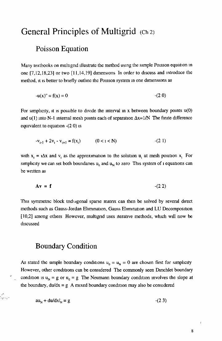
Many textbooks on multignd illustrate the method using the simple Poisson equation in

one [7,12,18,23] or two [11,14,19] dimensions In order to discuss and introduce the

method, it is better to briefly outline the Poisson system in one dimensions as

-u(x)" = f(x) = 0 -(2 0)

For simplicity, it is possible to divide the interval in x between boundary points u(0) and u(l) into N -l internal mesh points each of separation Ax=l/N The finite difference

equivalent to equation -(2 0) is

-vM + 2v, - v1+1 = f(x,) (0 < i < N) -(2 1)

with x, = lAx and v, as the approximation to the solution u, at mesh position x, For

simplicity we can set both boundaries u0 and uN to zero This system of i equations can

be written as

Av = f -(2 2)

This symmetric block tndi agonal sparse matrix can then be solved by several direct

methods such as Gauss-Jordan Elimination, Gauss Elimination and LU Decomposition

[10,2] among others However, multigrid uses iterative methods, which will now bediscussed

Boundary Condition

As stated the simple boundary conditions u0 = uN = 0 are chosen first for simplicity

However, other conditions can be considered The commonly seen Dinchlet boundary

condition is uN = g or u0 = g The Neumann boundary condition involves the slope at

the boundary, du/dx = g A mixed boundary condition may also be considered

auN + du/dxlN = g -(2 3)

where a is a constant

Discretization Error

The global error E can be defined as the difference between exact continuous solution

and the solution to the finite difference problem

E = llu(x) - u, 11 • -(2 4)

Equation -(2 1) assumes that the higher terms in the Taylor expansion of equation -

(2 0) can be ignored Hackbusch [12] has discussed the size of this in depth, but this

agrees m general with simpler approach of Briggs and McCormick [18], which

involves the truncation error t, given in the continuous equation,

Au(x) = Ax -2{ -u(x,_,) + 2u(x.) - u(x1+1) } + t, -(2 5)

A is the operator taken at position l on the continuous system If we assume that the

exact solution u(x) admits a Taylor series expansion about x,, then t, may be written as [18]

t, = A x V ^ - f ’Cx',)) -(2 6)

where x', denotes a point between x,_j and x1+1 It is possible to bound f'(x) using B by,

II f'(x) II <= B II f II -(2 7)

We must assume f is sufficiently smooth Then it is possible to bound the truncation error by

lit, II <= (Ax2/12)B Ilf II -(2 8)

Equation -(2 4) gives a relationship between the discretization error E and this truncation error t, as

AE = t, -(2 9)

which then gives E <= A 1 tj, which has been shown [18] to give

9

E <= C Ilf II Ax2/(12n2) -(2 10)

whereC~B This gives the bound for E as [1,7,18,23]

E <= 0(Ax2) -(2 11)

The general bound can be E <= O(AxP) [7] where p is the order of the differential

equation in question

The two most commonly used 'classical' iterative methods can be found in most

numerical, statistical and matrix mathematics texts These are the Jacobi and Gauss-

Seidel iterations, which for about one century were the only tools for solving small

linear systems iteratively These can be described as operating on a one dimensional

system of matrix form Av = b, giving the ith term as

They are also called linear stationary methods [1,12,18] However, the difference

between these methods is that the Jacobi method employs two separate v arrays and

doesn't overwrite existing elements m the v array but the Gauss-Seidel does overwrite

the previous elements in the v array as we sweep over l The storage required for

Gauss-Seidel is only one v array and is thus less than that of the Jacobi These methods are also known as relaxation methods and involve an initial guess at the solution They

then proceed to improve the current approximation by a succession of simple updating

steps or iterations, e g sweeps over i for equation -(2 12) The sequence of approximations v which is generated, should converge to the exact solution u of the

finite difference problem This convergence depends on whether a physical solution

exists to the corresponding analytical system, which can be tested by the existence of

A '1 Matrix A must be invertable if a solution is to exist Splitting or decomposing

matrix A into upper, lower and diagonal parts giving U, L and D respectively, we have

Iterative Methods

i-1 N I

(0 < 1 < N) - (2 12)

Av = (D - L - U)v = b -(2 13)

10

Then the Jacobi condition for convergence can be found from

vnew = D 1 (L + U )v 0id + D ' b -(2 14)

with

Pj = D 1 (L + U) -(2 15)

where Pj is the Jacobi matrix If written m the form of

vm+i = vm ' ®(Avm - b) -(2 16)

then B is referred to as a preconditioner The subscript m denotes the iteration

number The choice of preconditioner can then dictate the convergence properties [1]

Equation -(2 15) must satisfy the condition [1,2,12,14,18,20,23]

II Pj II < 1 -(2 17)

where the Euclidean norm of the Jacobi matrix Pj is taken,

II Pj II = (2 21 Py I2 ) 1/2 t -(2 18)

Brambles [1] has ngourously shown using the smallest and largest eigenvalues that for this condition to be satisfied, the eigenvalues of P,, A,(Pj) must satisfy

I W j ) U < 1 -(2 19)

where lX(Pj)lmax is the largest absolute eigenvalue and is called the spectral radius or

the convergence factor [2,7] In a Similar fashion, the convergence condition for Gauss-Seidel is found from rewriting equation -(2 12) as

v <- (D - L ) ' U v + (D - L ) 1 b

or

v <- Pv + g -(2 20)

with

11

Pg = (D - L ) 1U -(2 2 1 )

where the arrow [ 1,2,7] indicates replacement of v, as we sweep over l in an iteration

given by equation -(2 1) The requirement is again that

HPgll < 1 -(2 22)

or

a (P g)lmax < 1 -(2 23)

A hand waving argument for the conditions m equations -(2 17) and -(2 22) is given by

Briggs [7] from the general form of equation -(2 20) which is, v^1) = Pv(°) + g where

the superscript denotes the number of iterations This is the general form of methods

referred to as 'basic iterative methods', to which the Jacobi and Gauss-Seidel belong

The exact solution is u and u - v(n> = is the error after n iterative steps Using

equation -(2 20), we can write

u = Pu + g -(2 24)

Subtracting -(2 20) from -(2 24) gives e(') = Pe(°), which after n iteration sweeps

becomes,

e(") = p n e(°) -(2 25)

and thus we can write

lle^ll <= IIPIIn lle(°)H -(2 26)

This leads to the conclusion that if IIPII < 1, then the error is forced to zero as the iteration proceeds This leads to the definition of the contraction number z

[1,12,14,18,20,23], which is a function of iteration number n,

||e(n+D|| <= z (") lle(n)|l -(2 27)

12

If the limit of the norm IIPII with n goes to zero, then the method is convergent

However, this is only a sufficient condition [2,23] A necessary condition is that the

spectral radius of P is less than 1 [2,7,23] Other sufficient conditions are

1) Diagonal dominance [2]la j > 2 la,jl -(2 28)

2) A is real and positive definitexTAx > 0 -(2 29)

3) A is an M-matrix [2] (This was not used)

The Poisson matrix A wasn't diagonally dominant, was real positive definite and more

importantly it's spectral radius was found to be less than 1 (as expected) The error in

the approximation can be calculated after each iteration via u - v(n) = eW, and we can

obtain an error norm

Hell2 = ( 2 le,l2 ) 1/2

and plot this against iteration as in figure -(2 0)

However, since we don't normally possess the solution u, it is more practical to obtain

the residual norm llrll2 where the residual r is defined in the residual equation

r = Au - Av -(2 30)

Hackbusch [1] has demonstrated using the iteration matrix M, v = M(vm), that there is no fundamental distinction between convergence estimates for the error and

those for the residual, thus calculation of the residual will suffice Different types of Jacobi or Gauss-Seidel iterations appear if we sweep over l backwards from N -l to 1,

this will be referred to as a backward iteration, and the initial sweep as a forward iteration Alternating between these gives a symmetric iteration Another effective

alternative in the case of the Gauss-Seidel is to update all the even components first by

the expression

V2i = l/a2l2|{b21 - Za2lJvJ - 2a2lJvJ } and later sweeping over the odd points,

V 21+l = 1 / a 2 1+1 21+1 {^21+ 1 " ^ ^ l + i j V j " ^ ^ l + l j V j 1

13

Thus all even points are updated first, then all the odd points are updated This is

commonly referred to as a Red-Black iteration This has a clear advantage in terms of

implementation on a parallel computer Thus forward, backward, Red-Black and

ordinary/simple Gauss Seidel iterations can be combined together to give the

optimum results

Forward Red-Black Gauss-Seidel gives the best reduction in the residual norm or

error norm with increasing iterations Gauss-Seidel was chosen instead of Jacobi,

because of lower storage cost, and other reasons that will be discussed later

Plotting the residual norm for 100 iterations (figure -(2 1) we see that after around 10

or less iterations, the residual flattens, as does the error norm in figure -(2 0)

This is a limitation in most iterative methods By considering the Fourier aspects of the error as in the next section, we can develop ways to overcome this

Fourier Discussion

If we consider the basis set of eigenvectors of the difference equation matrix A, any

function in the space defined by the problem can be written in terms of this basis

The error or residual which are both linear, can be written in terms of these basis

14

Nearly all multignd texts [1,7,12,14,18,20,23] choose the Poisson case because it has

the advantage that its basis vectors are well known, and most importantly they can be

written as

v(x,) = I k sin(lkn/N) -(2 31)

where 1 is the point on the grid between 0 and N, and k is the mode This is in fact a

straight forward sine series, and can be used to describe the error Fortunately, this

corresponds to a sine Fourier analysis and from this we can see how the error behaves

with iteration, or more precisely, the relative strength of each of these eigenvector

elements can be observed with increasing iteration, due to the coincidence that these

eigenvectors for the Poisson case are in fact a sine series Another reason the sine

Fourier transform was chosen as opposed to the cosine or fast Fourier transform was because of the zero periodic boundary conditions, v0 = vN = 0 For the simple Poisson

case, Briggs and McCormick [7,18] have exploited the fact that the exact solution is

u(x)=0 for all mesh points Thus plotting v(x,) gives the error at each mesh point,

shown in figure -(2 2), after 100 iterations (notice only the lowest mode remains, e g

a sine wave)

F ractional Error Sine Fourier Transform of Error

Figure -(2 2) shows the error at each grid point, and figure -(2 3) shows the sine Fourier transform o f the error, both after 100 iterations Both suggest that only the low frequency errors remain, the lowest being the strongest, (a simple sine wave)

The magnitude of each mode k is given by the sine Fourier transform function [10]

(given in appendix A), and the result after 100 iterations is plotted in figure -(2 3),

where an equal amount of each mode was initially present (seen m the Fourier

transform as a straight line) It is then possible to control the initial guess in terms of

frequency content We can then set the initial guess to contain only one frequency We

can then repeat this for all the frequencies or modes, and observe how each is reduced

with increasing iterations Figure -(2 4) shows the number of iterations required to

reduce the residual to 1 % of the original

Error Mode P resen t in Guess

Figure -(2 4) shows the number of iterations required to reduce the error, for each individual error mode separately Less iterations are required to remove the high frequency error modes, where as more are needed for the lower frequencies

From these figures, it becomes evident that the lower k modes or 'smooth' modes are

difficult to remove, and this is in fact the reason why the residual or error fails to be reduced further, once the higher k modes or 'oscillatory' modes have been removed

Smoothing Properties

This property that-removes the high frequency modes but leaves the smooth, is

referred to as the smoothing property Thus our concern would be to find a mechanism

to reduce these smooth modes As we shall see later, this is achieved by the Coarse

16

Grid Correction Scheme Any iterative method that reduces the high frequency error

more so than lower frequencies is referred to as a 'smoother' The Gauss Seidel is the

most convenient and is often a very effective smoother [12] In order for the Jacobi

method to perform as a smoother, it must be weighted or damped [7,12,18], that is,

instead of replacing each new point v, with the new calculation, we add some of the

new to the old approximation for this point It will be explained later why it is essential

to have a smoother in a multi grid method Hackbusch [12] has defined a smoothing number gl which is close to the spectral radius, and can thus be used to approximate

this for small iterations, as the eigenvalues are not readily known, and there calculation

may prove as costly as the original problem This is a function of iteration number n,

a L(n) = sup IASI/|A | .(2 32)

Where S is a linear transform matrix such that, em+1 = S(em,b) Initially, o L(0) = 1 S

can be obtained after several iterations, thus this should indicate after several iterations

how the smoothing number decreases, as less high frequency modes are present A smoothing rate a b was introduced by Brandt [3], in terms of the kth eigenvalue A,k of

S,

o b(n) = sup max{ l?ikl(n) N/2 + i < k < N -l } -(2 33)

This also has an original value of 1 and decreases with iteration

Coarse Grid Correction Scheme

So far we have established that many standard iterative methods posses the smoothing property However the objective is to eliminate all frequency elements in the error (and thus the entire error) A good initial guess could improve the relaxation scheme, and a

well known technique for obtaining this is to perform some preliminary iterations on a coarse grid, and then use this as the initial guess on the fine grid

Instead of the sine founer transform, the fast fourier transform was used to described

the error after m iterations as

2n-l

£ c ma e ,(j6a) with 0 a = 7ta/n -(2 34)a=0

17

Orthogonality of {e'O^“)} [1,7,12,14,18,20,23] allows us to define an amplification

factor [23] g(0a), between each mth iteration as

Cma = g(0a)cm' a an<*

g ( 0 a ) = e ' 0 9 « ) / ( 2 - e ' 0 6 « ) ) - ( 2 3 5 )

Wesseling [23] reported that

lg(0«)l = (5 - 4cos0a) 1/2 -(2 36)

and giving the interval as h = 1/n

max'lg(0a)l = lg(0,)l = (1 + 20,2 + O(0,4) )m

= 1 -47t2h2 + 0 (h 4) -(2 37)

this is in general agreement with the spectral radius or convergence factor behaving as

[7,12,18] l-0 (h 2) It is possible that Successive Over Relaxation (SOR) method may

achieve maxlg(0a)l ~ l-O(h) for the Gauss-Seidel and Jacobi methods Both would then

suggest increasing h would give better convergence Also, iterating on a coarser grid

(with increased h) would prove less expensive since there are fewer unknowns to be

updated Recalling that most relaxation schemes discussed, have the common flaw of

preserving the low frequencies or smooth components in the error Assume that only

modes below k = N/2 are left The even points on the fine grid would be described on

the coarse grid as

This states that the kth mode on the fine grid (denoted by grid h) appears as low

frequency or smooth on this grid, but the same kth mode appears as a higher frequency

mode on the coarse grid (denoted by 2h) There was no reported advantage in using

grid spacmgs with ratios other than two [7,23], between fine and coarse grids This

ratio of two was found to be almost universal practice These higher frequency modes

on the coarse grid can then be eliminated by iterating on that grid.

This reasoning gives the advantage of either starting on, or transferring down to a

lower grid (restriction), and then transferring back to the fine grid (interpolation or

0 < k < N /2 -(2 38)

18

prolongation) Both of these terms are common in numerical analysis However,

should any high frequency modes remain after iterations on the fine grid, (k > N/2),

they are misrepresented on the coarse grid 2h as the (N - k)th mode, in a phenomenon

known as aliasing The effects of this can be later removed on the fine grid

We now make use of a very important relationship between the original problem, and

the residual equation, which is that, relaxation on the original equation Av = f with an

arbitrary initial guess is equivalent to relaxing on the residual equation Ae = r with the

specific initial guess e = 0 [7,12,18,23] It was this connection that prompted the

combination of this correction scheme and the transfer to the coarse grid

First, we iterate to remove high frequency modes then obtain the residual from f-Av =

r We then proceed to transfer the fine grid equation Aheh = rh to the coarse grid to

give A2he2h = r2h Further iterations on this equation will eliminate the high frequency

modes on this coarse grid We then interpolate the error e2h back onto grid h as eh, and

add it to the approximation v giving

vh = vh + eh -(2 39)

It now remains to be seen how we express or define grid transfer, both restriction to

lower and interpolation to higher grids Linear or direct restriction would simply

involve transferring all the even points of eh on the fine grid h to the points on the

coarse grid 2h, to give e2h, diagramatically shown in figure -(2 5), taken from Briggs

[7]

19

The general routine for this procedure is given by the C function Restnct() in

appendix A, which allows for the full weighting, or averaging between surrounding

points on the fine grid h Two possible approaches are possible, and the differences

will be discussed in the appendix C,

e2h, = >/4( vh,M + 2vh,, + vh,l+l ) 0 < i < N/2 -(2 40)

We can vary the degree of averaging of each of the surrounding points and this is

known as weighted restriction

For transferring the error e2h from coarse to fine grid, the function In te rp o la tio n )

shown in appendix A, uses linear interpolation given by

eh2l = e2h, 0 <= i <= N/2 - 1 -(2 41)

eV n = 1/r2( e2h, + e2h1+l ) -(2 42)

Briggs [7] has graphically illustrated this by figure -(2 6), where the black dots are e2h,

and the white dots are the interpolated points on grid h

In order for this linear interpolation to work, it is important that eh should appear as a

smooth vector on grid h with smooth modes as in figure -(2 7a), (black and white

dots), since high frequency modes cannot be represented on the coarse grid 2h except

20

by aliasing, and thus interpolation (between black points) would give a bad

approximation (for where the white dots should be), as shown in figure -(2 7b) from

Briggs [7]

We now need to define the coarse grid matrix operator A2h, which describes the finite

difference Poisson problem on the coarse grid 2h From equation -(2 2), which

describes the fine grid operator Ah, it becomes apparent that the interval Ax should

change from h to 2h, e g effectively double, since there are now only N/2 - 1 internal

mesh points on the grid 2h The grid on which a particular vector applies to is denoted

m the superscript This approach simply calculates A2h as if it were the initial problem,

except with interval 2h and N/2- 1 internal grid points This is referred to as the direct approach Another way of representing A on grid 2h is by the Galerkin

[1,7,12,18,19,23] representation This can be written in terms of functions as

A2h = Restnct(A h)Interpolate() -(2 43)

where the open brackets indicate that this operator will work on vector to the

right This is more commonly written as

A2h _ i h2h Ah j2hh or .(2 44)

A2h = RAhP -(2 45)

where we have defined the two operators m matrix form, R and P for restriction and

interpolation respectively This Galerkin method involves defining two matrices P and

R, thus using up extra storage, but does not require redefining the whole problem

matrix A on each level The Galerkin method may therefore costs less CPU time Since

almost all of the non diagonal elements in the matrices P and R are zero, it may also be

possible to make the product RAP an operation as opposed to matrix multiplication,

thus further saving on CPU time

It is now possible to present a general form for the coarse grid correction scheme

[1,2,8,52,53,54] using the Restricto and Interpolation() operators

1) Iterate V[ times on Ahfl1 = vh on the fine grid h, with the initial guess vh

2) Compute the residual for coarse grid 2h, r2h = Restrict(rh = f*1 - Ahvh)

3) Iterate v2 times (or in fact solve) A2he2h = r2h on the coarse grid 2h

4) Correct fine grid approximation, vh = vh + Interpolate(e2h)

5) Relax v3 times on Ahvh = f1 on the fine grid h

The three parameters v t , v2 and v3 can be chosen to give optimum performance as

discussed later It is important to consider the advantage of such a scheme again

Iterating on the fine grid will eliminate the oscillatory components of the error, leaving

a relatively smooth error Assume that we cannot solve the residual equation exactly on the coarse grid 2h, but do obtain a good approximation at the error Since this error

is smooth, interpolation will work very well and the error should be represented accurately on the fine grid

A program was written to implement a coarse grid correction scheme, and the results

after three or more iterations on both grids, agreed with those of Briggs [7], if equal

amounts of two initial modes are present

22

The Vcycle and other Multigrid Cycles

While on the coarse grid 2h, it is possible to perform another nested coarse grid

correction scheme, first finding the residual r2h, transferring this onto a coarser grid 4h,

via the restriction operator, Restrict(r2h) We then perform several iterations on the

equation A4he4h = r4*1 on the grid 4h We then interpolate the error, mterpolate(e4h) and

add this to the approximation e2h, e2h = e2h + Interpolate(e4h) It may also be possible

to solve e4h exactly, however this may not be necessary If nested coarse grid

corrections are applied m this manner until we reach the coarsest grid we can then

proceed upwards, continuously correcting the error on each level as above, until the

fine grid is reached again This basic idea is referred to as the Vcycle

As discussed later, for large meshes, this will prove more efficient than solving exactly

on the grid 2h Also it may not be necessary to descend to the coarsest grid Given a

mesh with N = 2q, having 2q -1 internal grid points, each again of separation h, the

coarser grid below this will have 2(q"l)-l points and a grid separation 2h, and so on as

we descend down the grids The coarsest grid is given by Lh, with L = 2^Q_|), where Q

> 1 The Vcycle procedure is the fundamental cycle in multigrid and can be found in

most multigrid texts Briggs [7] has summarised the Vcycle procedure as follows,

Iterate on Ahvh = f*1 vx times on the fine grid h with the initial guess vh

Compute r2h = Restrict(rh)

Iterate on A2he2h = r2h Vj times on the grid 2h with the initial guess e2h=0

Compute = Restrict(A2he2h - r2h)Iterate on A4he4h = v, times on the grid 4h with the initial guess

e4h=0

Compute r*h = Restrict(A4he4h - r*)

Solve on ALheLh = rLh on the coarsest grid Lh with the initialguess eLh=0

Correct e4h = e4h + Interpolate(e8h)

Iterate on A4he4h = r411 v2 times on the grid 4h with the corrected guess

e4h

Correct e2h = e2h + Interpolate^4*1)

23

Iterate on A2he2h = r2h v2 times on the grid 2h with the corrected guess e2h

Correct vh = vh + Interpolate(e2h)

Iterate on A h v h = fh v2 times on the fine grid h with the corrected approximation vh

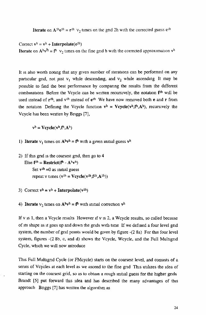
It is also worth noting that any given number of iterations can be performed on any particular grid, not just Vj while descending, and v2 while ascending It may be

possible to find the best performance by comparing the results from the different combinations Before the Vcycle can be written recursively, the notation f2*1 will be

used instead of r2h, and v2h instead of e2h We have now removed both e and r from

the notation Defining the Vcycle function vh = V c y c le tv ^ .A 11), recursively the

Vcycle has been written by Briggs [7],

vh = Vcycleiv*1,?1 11)

1) Iterate Vj times on Ahvh = tf1 with a given initial guess vh

2) If this grid is the coarsest grid, then go to 4 Else Ph = R estrict^ - Ahvh)

Set v2h =0 as initial guessrepeat v times (v2h = Vcycle(v2h,f2h,A2h))

3) Correct vh = vh + Interpolate^2*1)

4) Iterate v2 times on Ahvh = f*1 with initial correction vh

If v is 1, then a Vcycle results However if v is 2, a Wcycle results, so called because

of its shape as it goes up and down the grids with time If we defined a four level grid system, the number of grid points would be given by figure -(2 8a) For this four level

system, figures -(2 8b, c, and d) shows the Vcycle, Wcycle, and the Full Multignd Cycle, which we will now introduce

This Full Multigrid Cycle (or FMcycle) starts on the coarsest level, and consists of a

series of Vcycles at each level as we ascend to the fine grid This utilizes the idea of

starting on the coarsest grid, so as to obtain a rough initial guess for the higher grids

Brandt [5] put forward this idea and has described the many advantages of this approach Bnggs [7] has written the algorithm as

24

vh = FM cycleO h^A *1)

COMPUTE f^ph, ,

SET vh,v2h, to zero

v4h = v4h + Interpolate(v8h)

v4h = Vcycle(v4h,f4h,A4h)V2h _ v 2h + Interpolate(v4h)

v 2h = Vcycle(v2h,f2h,A2h)

vh = vh + Interpolate(v2h) vh = Vcycle(vh,f*\Ah)

This can be written recursively as

vh = FMcycle(vh,fh,Ah)

1) If this grid is the coarsest grid go to step 3

Else f211 = R estrict^ - Ahvh)Set v2h =0 as initial guess v2h = FMcycle(v2h,Ph,A2h)

2) Correct vh = vh + Interpolate(v2h)

3) vh = Vcycle(vh,ftl,Ah), v tim es

Notice that this calls the Vcycle() function, as well as itself recursively For any discretized stationary PDE problem, a full multigrid cycle FMcycle() with Vj and v2 = 3 is enough [19] to solve the equation Av = f with v =1, each time Vcycle() is called It is now apparent that the coarse grid correction scheme is the key part m the Vcycle(), and the Vcycle() is the fundamental cycle in all multigrid cycles The way in which each of the different cycles ascends and descends the grids is referred to as the multigrid schedule [23] There is no universal 'Black Box' multigrid algorithm that works for all systems [12], so each of these methods may be tested, for any particular given problem in question, to observe which performs best

Solve or iterate on the coarsest grid

25

-------------- * C - — — * — * — — * -----------* — — * ----------- — * r - — * --------------

■ X ■ /TS /Ts

----------------------------------------------* ----------------------------------------------------------------------------------------------------------------------------------- -

24- l pts

23- l pts

22- l pts

2 l- l pts

Four Level Gnd System a)

V-Cycle b) Full Multignd Cycle c)

26

Performance of the Poisson Equation

In order to discuss and compare the efficiency of all the above methods, both the direct

and the iterative, we must consider how much CPU time each of this would roughly

use It is common in multigrid literature to define a Work Unit (WU) [4,7,19] as the

amount of computational work done, or CPU processing time, as the work required to

compute one iteration or relaxation on the fine grid This has been put forward as the

golden rule of computation by Brandt (1982) [3,4,6], although the WU can be defined

differently As has been put forward a number of times by Brandt in a number of

publications, the WU depends not only on the type of method to be used, but the

choice of mathematical model used In general, many publications show that for a

given equation Av = f, it will cost at least several WU's to solve [23] If we consider

the Poisson equation for the simplest case, Av=0, with both boundaries set to zero, we

can plot the log of the error norm or residual norm against cycle, or now in this case

against the number of WU's performed

We will consider the computational cost of the WU's of for the Vcycle, Wcycle and the

FMcycle in accordance to the rough guide given by Bnggs[7] Consider a Vcycle with

v iterations on each grid while descending and ascending It is customary to neglect the

cost of mtergrid transfer operations which could amount to 15-20 percent of the cost of the entire cycle (for the Poisson case) On the fine grid there are v iterations, or v

WU's, then on the next coarse grid 2h there are 2_d times less, where d is the dimension

of the mesh Similarly on the grid 4h there are 4‘d times less The grid ph has p_d times

less Adding these together as an upper bound geometric series we get

1 Vcycle costs = 2v{l+ 2"d + 2~2d + +2~nd} < 2v ( l-_d ) W U's -(2 46)

The factor of two arises because we stop on each level twice Similarly the cost of a FMcycle with v iterations can be roughly given from this guide If the cost of a Vcycle

starting on the grid 2h is 2*d of the cost on the fine grid, then starting on grid 4h would cost 4 'd times as many WU's Any grid ph would then cost p 'd times less This results

in the series

1 FMcycle = 2 v ( - j - - 7 ){l + 2"d + 2~2d + + 2 “nd} < 2 v ( 1 W U's -(2 47)

27

It now becomes apparent that as the dimensions of the problem increase, we increase

the performance of multigrid cycles Using the above guide, a FMcycle m 1 -D would

cost 8 WU In 2-D the cost is about and m 3-D 5/2 In each case the definition and

the amount of work by each WU is different, but WU can be used to compare different

systems in this way

Using the above reasoning, it can be shown, that the series for the more complicated

Wcycle is given by

1 Wcycle = 2v{l + 2d (2“d) + 22d (2”2d) + + 2nd (2“nd)} = 2v{n} W U's -(2 48)

For six levels, in 1-D, with a total of 26-l points, we roughly surmise,

Vcycle WU < 4v

Wcycle WU ~ 12v FMcycle WU < 8v

The above has defined a work function as one iteration, which m turn is proportional

to N, for the Poisson case For the Poisson equation, it is not necessary to operate on

all the elements, only the tndiagonal elements It is known that all other elements are

zero Thus the iteration is given by

which is obtained from equation -(2 1) If this is performed for every ith point on the

grid, then it can be easily seen that for one iteration, we have two additions and one

division, e g approximately 3N operations, counting multiplication, division, addition and subtraction as one operation

However, if it is not known what elements are zero throughout the matrix, or if there

is no definite pattern, e g certain off diagonal lines are known to be non zero, then the

general matrix form of the Gauss-Seidel iteration must then be used as given by

equation -(2 12)

v, = V2( f(x,) + vM + vI+l) (0 < l < N) -(2 49)

i i N- 1

(0 < 1 < N) -(2 50)

28

Using this equation, and looking in more detail at the number of mathematical

manipulations required, one iteration now consists of

l 11) X ^ jVj having N/2-l multiplication and additions, gives N-2 manipulations

j= i

N- 1

2) ^ a v having N/2-l multiplication and additions, gives N-2 manipulationsj= i+ i

l - l N- 1

3) b, - ^ a ^ V j - £ a ljVj having two subtraction's for each ith termj=i j=i+i

l 1 N 1

4) l/a. { b, - ^ a y V j - ^S yV j } giving one division for each ith termj= i j= i+ i

5) the above repeated for each ith term, (repeated N times)

Summing from 1) to 4) gives 2N-1 ~ 2N operations, and this procedure is then

repeated for each ith term, e g N times, indicating that one iteration is now

proportional to N2, instead of the previous N for the Poisson case Equations -(2 46 -

2 48) now give

Vcycle cost in WU's < 8vN2 manipulations

Wcycle cost in WU's ~ 24vN2 manipulations

FMcycle cost in WU's < 16vN2 manipulations

The storage considerations involve storage for the problem matrix A, the solution v

and the RHS f on all levels In this case, even though most of the elements m A are

zero, we cannot identify a pattern as to which diagonals exist, why and where these will be in A, and thus cannot represent A by its diagonal elements Also, ionization

causes a further problem, as its elements, unlike all others are placed in a row For

these reasons, A was not represented by its diagonals, but left, as a sparse matrix

For a d dimensional problem, A has (N2)d or N2d elements, f and v have both Nd

elements The total is then N2d+2Nd, on the fine grid On the grid below this, this

29

quantity is reduced to (N/2)2d +2(N/2)d, or 2 '2d(N)2d +2(2‘d)(N)d The storage cost for

all levels can then be written as,

N 2d{l + 2~2d+ 2~ 4d + + 2~2nd} + 2 N d{l + 2 “d + 2 " 2d + + 2 ' nd}

< + 2 N i ( r - ^ ) - ( 2 51)

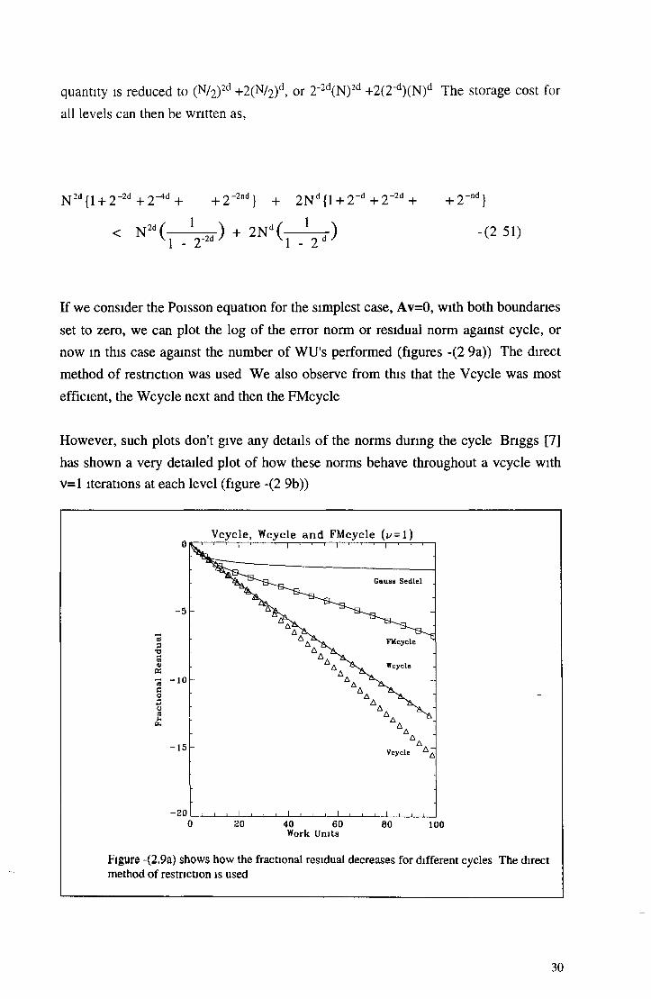
If w e consider the Poisson equation for the simplest case, A v=0, with both boundaries

set to zero, we can plot the log o f the error norm or residual norm against cycle, or

now m this case against the number o f WU's performed (figures -(2 9a)) The direct

method o f restriction was used W e also observe from this that the V cycle was most

efficient, the W cycle next and then the FM cycle

H owever, such plots don't give any details o f the norms during the cycle Briggs [7]

has shown a very detailed plot o f how these norms behave throughout a vcycle with

v=l iterations at each level (figure -(2 9b))

Vcycle, Wcycle a n d FMcycle ( y = l )

Work Units

Figure -(2.9a) shows how the fractional residual decreases for different cycles The direct method of restriction is used

30

In general agreement with this for the same simple Poisson case, figures 2 lOa-c, show

that if we increase n to 5, and then 10, the performance, or slope o f the curves

decreases The Galerkin method o f restriction was used, and this converges faster than

figure -(2 9a) using the direct method (for the Poisson case)

As mentioned before, when writing the code for the Restnct() function, it became

apparent that there were two possible ways to achieve this (ignoring the weighting

effect) These are to be referred to as Restnct(Ah) and Restnct(A2h) The difference

between them is discussed in the appendix C They give slightly different results, and

this will be discussed later W e have now looked at how the multignd program works

for our test Poisson problem Chapter one has introduced the form o f the Boltzmann

problem N ow we consider the application o f the multignd method The same

multignd algorithms will now be applied to the Boltzmann problem, and the results

observed

31

0Vcycle ( u = l , 5, 10)

f s J ' ' I 1 ••>• 1 1 ‘ ‘ 1 1 1 ‘ 1 i ' ' '

; ^ = 1 °- 1 0

*33■g55a>IX•3 -20ao

u = 5

oCOuU* A

-3 0

: v = l \

-4 0 1 1 1 1 1 ! 1 1 1 1 1 1 . 1 I 1 1 1 10 20 40 60 BO 100

Work Units

W cycle ( i / = l , 5, 10)0 \ ' ' 1 [ ' I 1 1 | 1 1 1 | 1 1 1 | 1 f"' '••V —

- 5: \ u ~ 1 0

*2 - ioto \ ...... 3 ....- .......uOSaeoo - 1 5«upt.

u - 5

- 2 0

" = 1 ^

- 2 5 ■ i i i i i i i j i i i i i i i i i iC 20 40 60 80 100

Work Units

Figures -(2 10a,b) show the effects of increasing v to 5 and 10, for the Vcycle and the Wcycle

32

Fra

ctio

nal

Res

idua

lFM cycle (u = 1, 5, 10)

W o r k U n i t s

Figure -(2 10c) shows the effects of increasing v to 5 and 10, for the FMcycle

33

Performance Results for the Boltzmann Case (Ch 3)

Multigrid Program for the Boltzmann Equation

The program M ultignd_Study c was developed from existing code which solved the

same plasma problem, except with a direct method, and by integrating forward in time

steps until a steady state solution was found This program solved the steady state

equations in matrix form given by A f=0 The program also explores the results o f

setting different multigrid parameters or multignd settings, to observe the best

convergence obtainable A more detailed listing o f these settings is given in the

appendix C Such multignd parameters would be for example, whether the mechanism

for restriction was weighted or linear, or if this was o f type AH or A2H (Chapter 2)

The type o f cycle used could be Vcycle, W cycle or FM cycle The level to which this

cycle descends to is referred to as the level, and how many iterations v are performed

on each level will all effect how the multignd method performs

The definition for the problem matrix A , can be given by either the direct approach, or

the Galerkm method The direct approach involves redefining the matnx A at each

level for that given number o f grid points, but with a different energy interval The

Galerkm method calculates A on the lower grids by the expression R A P given in

chapter 2 by the equations -(2 43,44,45)

The program contains macros for each of the corresponding settings These are all

given in the appendix A If these macros are true, then the program adopts these

settings If they are false, then the settings in question are not used

The program can repeatedly solve the problem for each different combination of

multignd settings or parameters and present the best results obtained This is achieved

by the Multigrid Operations section o f the code (discussed in appendix C)

The Main Program Procedural Flow

A list o f all the macro's related to the multignd aspects o f the program is given in the

appendix A A list o f input and output files is given also It is possible to set exactly

what the program does by setting macro's (m ost o f which are either set to 1 or 0).

Ongmally a third data file was used for this, but it was found more simple and

workable to use macro's for this purpose Appendix A also gives a listing and brief

explanation o f the prototypes o f all the functions in Multigrid_Study c and Cycles c

An overview o f the program flow is given here, and a more detailed account is

presented in the appendix C The first o f the two data files, b l7 dat is read, which

contains information regarding plasma parameters, and the size o f the problem q,

which would give 2q -1 internal grid points Memory is then allocated for the vectors

and matrices involved, whose size is now given The second data file xs dat is then

read This contains the cross-sections for all the collisional processes between

electrons and the neutrals, both elastic and inelastic The elements o f the matrix A are

now calculated, for each grid, in accordance to the multignd settings The boundary

conditions are also set, where the RHS can be made non zero as in equation -(1 13)

The problem is now defined, and the multignd solver now steps into play The set

problem can be solved again for a range o f multignd parameters given The

performance is then written to output files, indicating which multignd settings for the

same given problem have performed the best Thus multignd methods are being

compared, by experimentation, to find the optimum settings The simple flow diagram

given in appendix C shows how the above has been split into 7 blocks or sections of

code These blocks are discussed m more detail in the appendix C

Code Testing

The LU D solver, (achieved by the function Solve(), see appendix C), was tested on a

3x3 matrix It was then tested for the unique Poisson case, An = n' = 0, with only one

solution possible, n=0 only, given the two boundary conditions, n0=0 and nN=0 This

was tested for different sized meshes In the multignd case, where a solution exists on

each level, it was tested also The LU D solver was then tested for different boundary

conditions, and was found to function correctly

An effective method for testing the multignd code, is using cyclic reduction [2] This is

possible for the Poisson case, and if full weighted restriction is used, the solution can

be found by proceeding down and up the grids with zero error, or exactly zero

residual There is no reason why any multignd solver should ever give such an exact

result At first, it appeared that multignd was performing extremely successfully, but

by coincidence, the mechanism o f descending to the coarsest gnd with only one point,

and then ascending back to the fine grid, using only red-black (one is sufficient),

(forward or backward), Gauss-Seidel iteration on each level, and using weighted

35

restriction o f type A2H, corresponds, mathematically to the process o f cyclic

reduction This caused confusion However, this fact was used to test the multigrid

code, since successful cyclic reduction indicated that the code is working correctly, in

so far as the method o f descending and ascending to grids is correctly handled This

was found to be a useful test, when ever important fundamental changes were made to

the code The LU D solver could also be tested by inserting it at any level in the cyclic

reduction process, and solving on that level instead o f proceeding down further to

lower levels The residual still remained exactly zero The only explanation for this is

that both LU D and multigrid processes were functioning correctly

Several functions have been tested, particularly Residual() (see appendix C) which

calculates the residual in equation -(2 30), as this was vital in viewing the performance

o f multigrid Similar functions were tested which calculated the error norms These

were rewritten several times, using different methods, all o f which gave the same

result

The following notation will be used m the graphs, the number o f iterations on each grid

v, and the lowest level (referred to as the level) which the given cycle descends to, will

be denoted by, v , level ( e g 3,4 corresponds to v=3, level=4) The fine grid is level 6,

which contains 26- l internal grid points

If the type o f restriction is not mentioned, it is to be assumed that it is o f types AH and

LINEAR, since these generally give the best results for the Boltzmann case Unless

otherwise stated, it is to be assumed that the type o f Gauss-Seidel iteration is forward,

and basic/ordinary (not red-black) The figures produced, unless otherwise stated, are

the output o f the program M ultignd_Study c, which have been plotted by various EDL

software programs These programs read m the data from the output files, and plot

them accordingly

The Residual

It is almost universal practice in multigrid texts to use the residual as a measure o f the

performance o f the given solver in question Equation -(2 30) gives the expression for

the residual However, if we consider the matrix problem A v = f = 0, the absolute

value o f the residual is a factor o f the size o f the elements o f A , and f If the boundary

condition is set by making the first element f, on the right non zero, then the size of

this also effects the size o f the absolute residual

36

However, since the whole equation can be multiplied by any factor, then the size o f the

absolute residual itself is of no significance to the success or failure o f the method This

was the incentive for using a fractional residual, simply dividing the resulting absolute

residual by the initial residual At first glance one could assume that there should not

be any problem with this approach o f using fractional residual to monitor performance

The problem arises due to the observation that the residual results are not always

reproducible after the same number o f multigrid cycles, only because o f the arbitrary

boundary conditions and initial guess may be different It is not how close to the

solution the initial guess is, as clearly this will mean less work for the solver, but the

actual size or summation o f the elements in the initial guess It is found that fractional

residual may be a function o f the boundary condition and the initial guess, but there is

nothing to connect these two parameters, e g , for any given chosen boundary

condition, there could be any arbitrary initial guess size (£ fguess), and visa versa By

setting a boundary condition, this forces a unique solution, which m turn suggests that

the solution should sum to a given constant, Efsol (LUD) For the Boltzmann case, any

such problem does not arise unless f, is non zero, and the boundary condition is large

enough such that

I f sol (LU D ) > Xfguess -(3 0)

Multigrid however, for the Boltzmann case, even when a boundary condition is set,

proceeds to solve the problem to within a constant o f the actual solution, given by

LU D This is easily seen from figure -(3 0), which plots the multi grid and LUD

solution This is the case if the boundary conditions at both ends are equal [23], but the

left boundary has been set to non zero This is the case when both normalization's n(8)

and f(e) are solved for For the time being the n(e) normalisation will be chosen

Figures -(3 la-d) show that for the Boltzmann case, as the size o f the initial guess

becomes smaller than that o f the solution, from 1E+0 down to IE-6 o f its size, the

results becom e markedly worse (this is only seen in the levels lower than 5) The

multigrid solution is no longer solving to within a constant, as seen m figure -(3 0)

When the initial guess is IE-6 smaller than the solution, the shape o f this curve as seen

in figure -(3 0) cannot be superimposed onto the LU D shape, as it can when the initial

guess is 1E+0 and 1E+6 the size o f the LUD solution If the initial guess is 1E+6 larger

than the size o f the LU D solution, multigrid is seen to solve to withm a constant, as

figure -(3 0) clearly shows, and the corresponding fractional residual suggests that the

37

solver is converging just as successfully as it did when the initial guess was the same

size as the LUD solution This confirms equation -(3 0)

The problem is that if the residual is not reproducible for different guess size, and since

it depends on the relationship between two arbitrary parameters, the guess size and the

solution size (dictated by the boundary condition), then from this we cannot depend on

the residual to give a reliably account o f the performance However, equation -(3 0)

gives that the residual is reproducible for the Boltzmann case, once the arbitrary guess

size is larger than that o f the solution This is criteria by which the performance results

will proceed

Another indication o f performance is by setting a convergence criteria This will be discussed later, but this has its limitations

Different Size Initial Guess to that of Solution

Energy(grid pts)

Figure -(3 0) shows the multigrid solution when the initial guess size (Zfguess) is E+6, E+0, and E-6 that of the LUD solution size (EfS0,(LUD)) For E-6, the multigrid solution visibly appears different, and not withm a constant to the LUD solution

38

Log

of

Fra

ctio

nal

R

esid

ual

log

of

Fra

ctio

nal

R

esid

ual

Vcyc le , I n i t i a l G u e s s S u m s m a l l e r by 10° Vcyc le , I n i t i a l G u e s s S u m s m a l l e r by 1 0 “

A 1 61 4

-ill0 20 •11) fc>0 HO l l l l )

W o r k U n i t ' s¿I)

V c y c l e I n i t i a l G u e s s S u m s r n a l h t I>v 10

A

A

A

4 t- * + + I I f t t f & $A A A A A A A 1 5

l¿<)

-öl0 ¿o <10 6 0 HO

W o r k U n i t s1 00

V c y c l c I n i t i a l G u e s s S u m s m a l l e r b> 10

Work U n i t s W o r k U n i t s

I ¿0

1 ¿0

Figures -(3 la-d) show that for the Boltzmann case, as the size of the initial g u e s s becomes smaller than that of the solution, from 1E+0 down to IE-6 of its size, the results become markedly worse (this is only seen in the levels lower than 5)

This size indifference between the guess and solution, is solved by normalizing the size

o f the approximation to that o f the solution after each cycle However, this defeats the

purpose o f the objective, in that the solution is unknown to the multignd solver, as is

its size (Efsol(LUD) ) It is found that by doing this, the residual will continue to

decrease down to the order o f IE -15/-16 This will be discussed later

The Vcycle is the fundamental cycle in multignd, from which all the other cycles have

be constructed from For this reason, we first consider its performance, as if this is bad,

then the other cycles will tend to follow suit

Figure -(3 2) shows results for the different types o f restriction (AH or A2H, LINEAR

or WEIGHTED) From this we see that the CGCS (Coarse Grid Correction Scheme,

e g Vcycle to level 5), denoted by 1,5, 2,5, and 3,5, gives the best performance If the

multigrid method was working correctly, the cycles to lower levels should at least

perform better than the CGCS However, level 4, 1,4, and 2,4 both fail, and 3,4 barely

achieves anything better than that given by the Gauss-Seidel iteration (denoted by GS)

This suggests that at least v=3 is required to give a reasonable improvement on the

convergence o f the Gauss Seidel This is not in accordance with the general multignd

theory The Vcycles 3,3 only converges if the restriction types are AH and

W EIGHTED All other 3,3 Vcycles fail or tend to perform worse than the Gauss

Seidel, and are thus clearly failing All cycles to lower levels fail Vcycles 3,4 A2H,

LINEAR and 3,4 A2H, W EIGHTED also fail AH 3,4 LINEAR and WEIGHTED

both converge, but not veiy convincingly The fact that the CGCS performance shown

in figure -(3 3) is better than the previous figure -(3 2), and that the Vcycle fails on all

lower levels indicates that multigrid is not performing in the correct expected manner

At this point, we could speculate that perhaps something is occurring wrong on the

lower grids The code was tested, and was found to work for the Poisson, and the

cyclic reduction testing as mentioned before This testing suggests that it is not the

multignd code mechanism that is at fault This code is in fact doing what is asked o f it

Figure -(3 3) shows that AH, LINEAR 2,5 gives almost an identical result as AH,

W EIGHTED 2,5, thus indicating that for CGCS, the types LINEAR and W EIGHTED

have little or no significant effect on the results The type A2H however may give a

different result than that o f AH Another concerning issue is the manner in which the

residual seem s to flatten out in figure -(3 3), at around fres=10'6. This is not small

enough to be o f the order o f the round o ff error that the double precision code uses

The residual for the Poisson case has been observed to converge to 10'25 or more, and

40

has not been seen flattening out in this manner The Gauss-Seidel iteration, if

continued for several hundred iterations, will give a continuously decreasing residual,

where flattening has not been observed as in the case o f CGCS or Vcycles to lower

grids Thus the problem is definitely associated with the lower grids As the coding

mechanism is functioning correctly, perhaps the representation o f the problem on the

coarse grids is at fault in some way This was checked in great detail several times, and

is believed to be representing the problem m the required manner in accordance to

multigrid procedure

Vcycle, Type AH, A2H, Linear, and Weighted

Work Units

Figure -(3 2) showing the different types of restriction methods, for the Vcycle, for various different v and level of descent

41

Vcycle, with different types of Restriction

Work U n it s

Figure -(3 3) showing the different types of restriction methods, for the Vcycle, for various different v and level of descent AH, LINEAR 2,5 gives almost an identical result as AH, WEIGHTED 2,5, thus indicating that for CGCS, the types LINEAR and WEIGHTED have little or no significant effect on the results

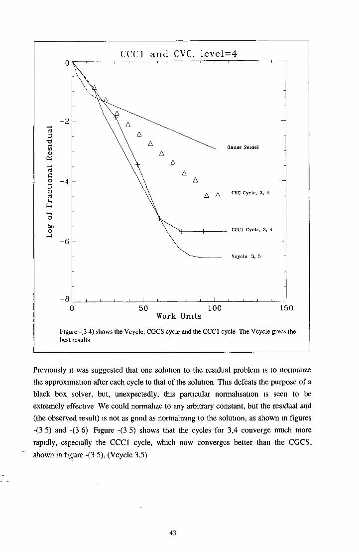
Figure -(3 4) shows that the nearest performance to the CGCS is the CCC1 cycle, 3,4 which involve a Vcycle to level 4, follow ed by a Vcycle to level 5 Again this indicates that the problem o f the lower grids is apparent on level four

42

CCC1 a n d CVC, l e v e l = 4

Work U nits

Figure -(3 4) shows the Vcycle, CGCS cycle and the CCC1 cycle The Vcycle gives the best results

Previously it was suggested that one solution to the residual problem is to normalize

the approximation after each cycle to that o f the solution This defeats the purpose o f a

black box solver, but, unexpectedly, this particular normalisation is seen to be

extremely effective W e could normalize to any arbitrary constant, but the residual and

(the observed result) is not as good as normalizing to the solution, as shown in figures

-(3 5) and -(3 6) Figure -(3 5) shows that the cycles for 3,4 converge much more

rapidly, especially the CCC1 cycle, which now converges better than the CGCS,

shown in figure -(3 5), (V cycle 3,5)

43

N o r m a l i z e d to LUD S o lu t i o n , v - 3, level = 4

Work Units

Figure -(3 5) shows the different cycles with normalization after each cycle This shows the failure of the FMcycle and the Wcycle

N o r m a l i z e d , V c y c l e C G C S a n d C C C 1 C y c l e

Work Units

Figure -(3 6) shows the CCCl Cycle, for different v and level, with normalization after each cycle

These results are not possible however, unless the solution (or its size is known) It is

however not possible to find the size (£ fsol) without knowing the solution These

results tell us that the multigrid solver is converging to within a constant, or that the

solution is o f the wrong size to that dictated by the boundary condition The LUD size

(S fso|(LUD)) is the exact size dictated to it by the boundary condition, and thus the

size o f its solution gives the lowest possible residual, lower than any other size (Zfso!)

If the multigrid solver solves to within a constant, then if we test the residual o f its

result with boundary condition equal to zero ( giving the infinite solution problem), or

having f0=0, it could be expected to be better However, the residual result was

identical to the case when f0 is non zero, because o f the negligible effect that a non

zero f0 had m the calculation o f the residual This suggests that the presence o f a non

zero f0 has little or no effect on the multigrid solution (provided that we conform with

equation -(3 0), and as a result, we cannot force the desired multigrid solution towards

any size by setting the boundary conditions Thus the fractional residual can be

changed by normalizing the solution This tells us that the actual values o f fractional

residual obtained, don't in fact indicate an exact measurement o f performance, but act

just as a guide line H owever, following the criteria given by equation -(3 0), all

fractional residual plots are reproducible, and their relative performances can be given

by their relative values o f fractional residual in the plots Since multigrid can only solve

to within a constant o f the LU D solution (which offers the best results), the multigrid

solution must be normalized to that o f the LU D m order to obtain the error norm, or

maximum error The absolute value o f the error norm (or maximum) gives a realistic

and quantitative assessment o f the performance

The above results, which indicate problems on the lower grids, acted as an incentive to

recode the problem, such that it would solve for f(e), instead o f the previous

normalisation n(e) Figure -(3 7) shows that when solving for f(e), the performance of

the CGCS is identical as is the CCC1 cycle 3,4, to the n(e) choice H owever, one small

insignificant difference was observed in that the CVC cycle 3,4, for f(e) is not as

effective as it is for n(e) After observing other results, it was apparent that this

recoding did not appear to remove the problem on the lower grids, as this problem was

still present with the f(e) normalisation

In an attempt to improve the unexpected bad performance results so far, several

different adaptive iterations were considered, and the choice o f ascending (forward)

Gauss-Seidel was revised Red-black Gauss-Seidel is not as good a smoother as the

basic or simple Gauss-Seidel, and ascending through the unknowns (forward) always

45

appeared to give better results than the choice o f descending through the unknowns

(backward)

If we consider the residual equation, this equation -(2 30) r = A v - f, depends on the

size o f the solution v The exact LUD solution for v, for the choice o f energy interval

de = 4ev with 26- l internal points, (which has been used so far), scales 11 orders of

magnitude

Solving for f(e)

0 50 100 150W ork U n it s

Figure -(3 7) solves for f(e) instead of n(e) The problem on the lower grid still remains

Figure -(3 0) shows that the first sixth o f the curve contains the mam peak o f electrons,

and it is this larger part o f the solution that is more important in the residual equation,

as this larger part dictates whether the fractional residual appears good or bad If we

obtained a better solution for this region, the fractional residual would appear good,

almost regardless o f how the multignd solution is behaving for the rest o f the curve

This point was tested by creating an iteration that updated this the first one sixth o f the

multignd approximation, and then proceeded to update the entire approximation Thus

more emphasis was placed on this larger region o f the curve Figures -(3 8) and -(3 9)

46

give the best illustration of the adaptive case, for the case o f some failing Vcycles 2,3,

2,4, and 3,3, the adaptive iteration can improve the error norms (the fractional residual

was in fact greater than unity, which clearly suggests failure m these cases) The

adaptation o f updating approximately one sixth o f the points was found to give the

best results This adaptation was only found to be really effective if implemented as the

Vcycle ascends, and omitted as the Vcycle descends Also, a similar adaptation on the

lower grids was found to give slightly better results, if one iteration consists of

updating about one quarter o f the points, and then all the points, again putting more

emphasis on the larger points, which in fact turn out to be in the same region o f the

curve as those on the fine grid More results from the adaptive case will be discussed

later, but the adaptive case has not in any way eliminated the main problem as to why

the multigrid solver fails when it incorporates the lower grids into the cycle

A dap tive V cy c le s

W o r k U n i t s

Figure -(3 8) shows the Vcycles with the adaptive iteration , improving results, (compared to figure -(3 9) below) but not removing the problem occurring on the lower grid

47

Log

of

Fra

cti

on

al

No

rma

liz

ed

E

rro

r N

orm

Non Adaptive Vcycles

W o r k U n i t s

Figure -(3 9) shows that the same Vcycles as in figure -(3 8), but without the adaptive iteration

48

The Galerkin Restriction method however, if used instead o f the previous direct method,

shows more promising results The main difference being that this method doesn't require

that the level be as high as 3 or 4, or that v be as high as 2 or 3 Unlike the direct method,

the CGCS is not the most or one o f the most effective results, e g Vcycles with level=5

Multigrid theory clearly states that it is more beneficial to descend down to lower grids

Figure -(3 10) shows that going down to level four or lower achieves a much better

performance than the CGCS This was perhaps the major problem with the direct method

There seemed no reason why a Galerkm method should work, while this should fail

RAP V cycle, u = l , vary in g lev e l

W o r k U n i t s

Figure -(3 10) shows that going down to level four or lower achieves a much better performance than the CGCS

When v = l , leve l= l, figure -(3 10) shows that the Galerkin method produces the best

results This, (in contrast with the direct method), agrees with multigrid m general There

is only the problem or question regarding the flattening out o f the residual, somewhere

between IE-6 and IE-7 The error norm and maximum error also flatten out after the

same number o f W Us This will be addressed later The more appropriate question to ask

now, would be as to why the direct method appears to fail, while the Galerkin method

succeeds The fact that both succeed as expected for the Poisson case, suggests that the

code is functioning correctly This was looked into further, and this was in fact the case

No preferred method for restriction between either o f these had been previously suggested

in any multignd text or publications, only that both would be expected to succeed for all

problems, not one or the other

If we consider the direct method first, the problem matrix is defined for level q, for 2q -1

points It is then defined on level q-1 for 2q' ‘ -1 points, and so on down to level 1 The

data file, containing the cross sections, also contains the threshold energies, o f which there

are, for example, four in the case o f a plasma consisting o f N 2 m olecules, tw o electronic

excitations, one vibrational and one ionisation The cross sections are-given in eV , and

must be converted to points on the grid, which are equally spaced Thus, if the problem

matrix is to be redefined on each level, corresponding thresholds must also be redefined

for each level This was achieved in such a manner so as to obtain thresholds similar to

those obtained if the problem had been defined initially on that lower grid Given that there

are four threshold energies in the data file, a one, three or seven grid system would only

contain 1 or 2 o f those four thresholds, thus the system would be different Also, the

whole physical concept o f redefining the system with 1, 3 and 7 energy points is not quite

convincing Clearly there are not enough energy points to make up a system which m any

way represents the original one By redefining the problem with less points, because o f the

thresholds, it is as though we are defining a different system In contrast to this, the

Galerkin method simply manipulates the fine grid matrix A, by finding R A P (equation -

(2 45)) to give A for the next lowest grid, and so on down the lower grids The matrices R

and P contain simple fractions Threshold information is not lost in this manner Nothing is

redefined for a smaller number o f points, and all the information that exists in the original

problem is still preserved in A for the lower grids This is the suggested reason for the

success o f the Galerkin method, and the failure o f the direct method

Figure -(3 10), also shows that there is little or no difference between descending to level

1, 2 or level 3, although level 1 is slightly better These however perform better than level

4 This seems to indicate that work done on grids 1 and 2 don't seem to contribute much

to the general scheme o f things This does comply with multigrid theory

50

V

A sub routine was incorporated into the program from Numerical Recipes in C [5], in

order to obtain the eigenvalues for the matrix A It first finds the inverse, using the Gauss

Jordan method, and then proceeds to numerically calculate the eigenvalues Each

eigenvalue corresponds to an eigenvector, and the set o f eigenvectors can define any error

vector e, which gives the difference between the exact solution u, and the approximation

v The effect o f continuous Gauss Seidel iterations applied on the approximation v, for the

problem A v=f, effectively remove the oscillatory or higher frequency eigenvector elements

o f the error e This is the smoothing effect o f the Gauss Seidel iteration By calculating the

eigenvalues for the problem matrix on all levels, it was found that for the particular choice

o f 26- l points, and with de= 4eV , the maximum eigenvalues for levels 4 or lower were in

fact greater than unity This does not conform to the required convergence condition given

by equation -(2 23), lA,(Pg)lmax < 1

This indicates that the Gauss Seidel iteration cannot converge on these grids, since the

maximum eigenvalue is greater than unity Although it was not possible to obtain plots of

the eigenvalues for each mode present in the error, or study the actual size o f each

eigenvalue element o f the error, we know that for the Gauss Seidel case the largest

eigenvalue is given by the low est frequency mode [7] This is probably the case for the

Boltzmann case, and if any o f the lower eigenvector modes have corresponding

eigenvalues larger than one, this means that these eigenvector m odes (error elements)

cannot be removed by the Gauss-Seidel iteration However, multigrid does not require

that the lower frequency modes be completely removed, only on the coarsest grid, and this

is perhaps the reason why multigrid works even though convergence is not possible on

levels 4 or lower Recalling the observation that for the Boltzmann case, multigrid,

regardless o f the fact that the boundary conditions force a unique solution, only solves the

problem to withm a constant, we can speculate that if the low est frequency could not be

removed by multigrid, then it would perhaps be observed as a smooth component, (we

don't know the form or shape o f this mode), and on a Log scale this could possibly appear

as a constant value error, e g the muhtgnd solution appears to have solved to withm a

constant, but perhaps this is in fact the lowest frequency mode, or a combination o f some

low frequency m odes which could not be removed by multigrid because the maximum

eigenvalues on levels four or lower are greater than unity

Figure -(3 11) shows the Galerkin method (using R A P, as in equation -(2 45)) for the

Poisson case, with v = l , and level= l-5 There is definitely an advantage in descending

down to the lower levels, in particular, the lowest level

51

This is the type o f multigrid behaviour we would expect in figure -(3 10), but there is no

real advantage m descending below level 3 However, the slope o f these performances are

better for the Boltzmann, for the first 25 W U or so, and then the fractional residual

flattens out This behaviour is not seen in the Poisson case, again in this respect, w e would

not expect this flattening out for multigrid behaviour Could it be possible to attribute

these bad elements to the eigenvalue size on lower levels7

Figure -(3 12) shows that LINEAR restriction worked better than W EIGHTED, and when

restriction type A2H is used, the method fails completely The best results so far are then

given in figure -(3 10), with 1,1 (v = l, leve l= l)

52

RAP Vcycle, for B o l tz m a n , v - \

W o r k U n i t s

F igure -(3 12) show s that for the B oltzm ann case, the V cycle w ith RAP (G alerkin m ethod o f re s tr ic tio n ) , L IN EA R restriction w orked better than W EIG H TED

Instead o f using either type A2H or AH for restriction, the matrix operator R can be

employed [7,18,23] The matrix operator P can be used for interpolation Since, however

most o f the elements in both these operators are zero, there is a lot o f wasted calculation,

compared to the previous AH and A2H Figure -(3 13) shows that the results o f this are

slightly better than figure -(3 10), where the fractional residual flattens out around 20 W U

as opposed to 25

53

RAP Vcycle, f o r B o l t z m a n n , v = l , l e v e l = l

Work Units

Figure -(3 13) shows R A P (Galerkin m ethod) Vcycle, using R and P instead o f A H or A2H m ethods

If the error norm or the maximum error is plotted instead o f fractional residual, as m figure

-(3 13), w e see that the magnitude is o f the same order o f fractional residual A lso the

behaviour is identical, e g both errors flatten out after exactly the same number o f W Us

After this point, there seem s to be no advantage in continuing the method There is also no

advantage m reducing the order o f the error smaller than the discretization error E <=

0 (h p), [1 ,7 ,18,23], where p is the order o f the differential equation, 2, and h is the size of

the interval, such that all intervals add to 1 For the present q=6 case, h = l/6 3 , and E = O

lO^-lO'5 Figure -(3 15) shows that to reduce the order o f the error, to 10^-105, requires

around 6-9 W U It is not necessary to progress further than this, and from this point of

view, the method is a success The problem o f the flattening out o f fractional residual or

error does not effect the practical application o f the result

54

Figure -(3.14) show s the fractional residual after 15 W U 's, for different v. F igure -(3.15) shows (m ore clearly for 28- l points), how v = l is the best choice in agreem ent w ith the previous figure.

V - C y c le v , l e v e l = l , 2* p t s , f o r d i f f e r e n t u

G a u s s S e d i e l

- 6 L ^ i i i L , i i i I i i i i I i i— i— 10 5 10 15 20

Work Units

15 WUs, for d i f f e r e n t v

Vcycle, Wcycle a n d FMcycle (2* pts)

F igure -(3.16) shows again that the V cycle offers a better perform ance than any other type o f cycle (for 28- l points).

55

Both the calculation of the maximum error and the error norm, involve knowledge o f the

solution, which, o f coarse is not readily available Apart from calculating fractional

residual, another, perhaps even less costly way of predicting the point where this flattening

will occur is to calculate the fractional change in each f, on the approximation from its

previous value, given by (fj-fj.j)/^, and continuing the method until this quantity is smaller

than some suggested value,

(f1-f1. 1y f1 < p - ( 3 1)

Figure -(3 14) shows the residuals o f different v after 4 Vcycles, 15 WU's The choice o f

v = l is clearly the best for levels= l,2 ,3 ,4 The choice o f either level =1, 2 or 3 as

mentioned before, appears to make little difference, only that all are better than descending

to level 4 Figure -(3 15) also shows quite clearly that for around the first 30 WU's, with

level= l, the best choice o f v is 1 (more clearly seen for 28- l points) This agrees with the

Poisson case and that reported [1,7,18,23]

Figure -(3 16) shows that the Vcycle offers a better performance than any other type of

cycle The poor performance o f the fm la and fm lb FM cycles (exact definitions given in

appendix C) is concerning, as most reports suggest that the full multigrid cycles are more

efficient than the Vcycle The Vcycle was also found the most effective for the Poisson

case, again not agreeing with Briggs, Brandt or W esseling [7,23,3]

Efficiency

The only solvers that in two or more dimensions can perhaps be comparable to the speed

o f the multigrid solvers is the direct solver based on the Fast Fourier Transform, but these

are more limited than multigrid and cannot be compared for very large meshes

McCormick maintains that the efficiency o f full multigrid cycle attains the same efficiency

for the general nonlinear, not necessarily elliptic problems as in the case o f the two

dimensional Poisson equation, but for any boundary condition problems, eigen problems,

and for problems including free surfaces, shocks, reentrant com ers, discountious

coefficients and other singularities Unfortunately, the full multigrid cycle appears to be

less effective than the Vcycle, so fast methods may be at least comparable to the multigrid

56

method for the Boltzmann case. The Vcycle must be reapplied again and again until the

desired accuracy is maintained.

The required reduction in error is such to give an error norm of around the same size as

the truncation error due to finite differencing with spacing h [1,7,18,23]

u - v = e ~ Kh2 = K(i/n)2 = K(i/2q)2 = K2"2q -(3.2)

where K is constant. The error norm e is to be reduced to around this amount for a q level

system with 2q points. Figure -(3.17) plots, (as we increase the number of points), the

number of mathematical manipulations required to reduce the error norm in accordance to

equation -(3.2). This curve is based on the calculation of 2N2 manipulations for one fine grid iteration (or 1WU), and just under 3WU's (6N2) for one Vcycle, (v= l, level=l), (A

more accurate calculation will show that this is 2.66WU’s, however, we have neglected

intergrid transfer work estimated at around 15% or more of 1WU, which will bring this to

around 3WU's). The choice of K has little effect on this curve for the multigrid case. It can

be seen that for q > 6, multigrid becomes cheaper than the direct LUD method.

Figure -(3.15) shows that for 2-3 Vcycles with v=l and level=l to 3, will reduce the error

to the order of around lO^-lO'5. The direct LUD method requires >/3N3 manipulations, as

opposed to the 2N2 required per iteration, which gives the definition of 1WU. The number

of WU's required for the direct method then becomes around i/6N, for q=6, this is around

10.5WU's. Two Vcycles costs less than 6WU's, and thus the multigrid method is cheaper

once i/6N WU's in the direct method is larger than 6. This is little improvement on the LUD case of 10.5WU's.

The 6WU's required for two Vcycles takes into consideration the work required for inter­grid transfer, which for the Boltzmann case is less than the estimate of around 15-20% of

the work done per V-Cycle [7] for the Poisson problem, since the cost of one WU is more for the Boltzmann case. This is because of the there are more of diagonal matrix elements

for the Boltzmann case.

If q=8, then */6N is around 42WU's. However, the truncation error is now 0 0 /256)2 ~10'5,

and an error less than 1 O'5- 1 O'6 is now required, which in turn requires more WU's than for

the q=6 case. The number of Vcycles required now becomes, 3-4, to reduce the error to

1O'5- 10~6. This costs around 9-12 WU's (where WU is defined as one iteration on the fine

57

grid with 28 - 1) For 2 '°- 1 points, this error becomes of order 106 However, it is still

possible to achieve this before the residual flattens out Thus for q > 6, multignd has a

clear advantage over the direct method, and more so as both the size N, and the number of

dimensions of the problem increases

LU D ec o m p o s t io n and Multigrid Vcycle

G rid S iz e q (N = 2 ^ )

Figure -(3 17) shows, as we increase the number of points, the number of mathematical manipulations required to reduce the error norm in accordance to equation -(3 2)

58

Conclusions

The residual was not reproducible after the same number o f multigrid cycles, only because

o f the size (£ fguess) o f the initial guess relative to the size (Zfsol) o f the solution given by

the LUD solver The fractional residual was only found to be reproducible once equation

-(3 0) was satisfied

I f sol(LU D ) > -(3 0)

This is unlike the Poisson case Multigrid for the Boltzmann problem only solved to within

a constant o f the solution, regardless o f whether the problem had an infinite series solution

or a unique solution However, multigrid only does this if the equation -(3 0) is satisfied,

otherwise it is clearly seen to fail for the Boltzmann case The direct method was looked at

first for all four combinations o f the restriction types AH or A2H and LINEAR or

W EIGHTED The Coarse Grid Correction Scheme (CGCS, Vcycle descending only one

level), was found to give the best performance Descending to lower grids decreased the

performance, and for a 6 level system, descending below level 3, and in some cases 4

resulted in failure o f the method A value o f v = l also caused the method to fail, and

neither o f these observations agrees with multigrid theory All cycles appear to stop

converging somewhere between a fractional residual o f 10'3 and 10"6

If the approximation is normalised to that o f the LUD solution after each cycle, this results

in much faster convergence However, the size £ fsol (LUD) is then required, and thus the

solution needs to be known, which then defeats the purpose Normalising to other sizes

(unity for example) tended to give non reproducible results depending on both

£ fsol(LUD), £ fguess, and did not result in the any reproducible improvement in

convergence

Provided we conform to equation -(3 0), multigrid proceeds to converge to within a

constant When the problem was defined for f(e) instead o f n(e), the results were similar

The problem o f a failing method on the lower grids still occurred

The ordinary Gauss Seidel forward iteration was found to be a better smoother than Red-

Black Gauss Seidel, or backward iterations

59

An adaptive iteration was developed which updated the first one sixth o f the multignd

approximation, and then all the points on the approximation This focused more on the

larger part o f the electron distribution, as this larger part dictates the results in the form of

the fractional residual and the error norms This adaptive iteration improved convergence,

but did not remove the problem on the lower grids This adaptation was only found to be

effective if implemented as the Vcycle ascends and omitted as it descends Similar

adaptations to the basic iteration for the two lower grids also improved performance

The Galerkm method o f restriction gives better convergence than the direct method for

the Vcycle With the Galerkm method, the optimum choice o f v = l is in accordance with

convergence estimates for similar second order differential problems Also, incorporating

the lower grids into the cycle increases the performance for the Galerkm method, where as

for the direct method, this reduces the performance, and if incorporating grid levels 3 or

below, the method fails The Galerkm method is seen to behave as expected, apart from

the flattening out o f the residual (where convergence stops)

The Galerkm method employing R and P worked better than AH /A2H and

LINEAR/W EIGHTED restriction methods, but uses more storage space

The value o f lX,(Pg)lmax for the iteration matrix Pg was found to be larger than unity for the

Gauss Seidel iteration on the lower grids, indicating that the iteration can not converge on

these levels It is suggested that lA,(Pg)lmax is probably the k = l eigenvalue or lA,(Pg(k=l))l

This corresponds to the low est frequency eigenvector If this is the case, then it is this

element o f the error that cannot be removed This is the suggested reason as to why

multigrid for the Boltzmann stops converging, and the error norms or the fractional

residual flattens out

The Vcycle performs better than any other cycle, including the FM cycle This is

concerning as it is not in agreement with Briggs, Brandt and other texts [3,4,6,7,23] We

might however expect the V cycle to perform better than the W cycle

Fortunately, multignd converges to the discretization error E <= 0 (2 '2q), before it stops

or seizes to converge, for systems o f point size 2q- l , for q = 6 to 12 From this

perspective, the method achieves what is asked o f it before it seizes to converge, as there

is no benefit m converging to below the size o f the discretization error Thus the problem

o f the flattening out o f the residual docs not cffect the practical application o f the result

60

Multigrid methods are more favourable than direct methods given the accuracy required

for the Boltzmann problem For q>6 multigrid becomes cheaper than the direct LUD

method, when just enough Vcycles are applied to converge down to the same size as the

discretization error For a 26 points problem, multigrid only requires around 60% of the

time needed by LUD For a 28 points problem, multigrid requires around 20%, and for 2 10

points around 5 % The reduction i n work load is also seen with increasing dimension

The multigrid method is less specialised than existing fast solvers, and in the case of the

Boltzmann problem has the advantage that the method can be manipulated to cope with

the non-linear case involving electron-electron collisions This can then be solved, with no substantial loss in efficiency

61

APPENDIX

Appendix A

This appendix contains more information about the C source code, and some

guidelines for the program M ultignd_Study c A macro listing is given, and the

purpose o f each function is given beside each C function prototype A program listing

o f all the C source code, and header files is given on an attached disc, along with a

makefile, used to com pile these source programs The original program reads from two

input files, b l7 dat, which used the file pointer infile, and xs dat which used the file

pointer xsfile The results file for the plasma properties is b l7 res, which uses the file

pointer outfile All other files begin with fp, followed by the file name, and have the

extension dat All file pointers also begin with fp and contain the same name as the

files, omitting the dat extension Also, Write() functions should usually indicate by

their name what file pointer they are using, and output file they are writing to

List of Multi grid Output Data Files

Below is a list o f multigrid output files, the purpose o f which to view multigrid

performance under different settings

fpbc dat Records the area under the solution with the boundary condition

fpcoarse dat Records the solution and approximation at every grid level

fpcycle dat Records the fractional residual and other parameters

with increasing cycles, for all cycles chosen

fpdfmax dat Records the maximum difference between the previous ith point

and the new ith point in the multigrid approximation, as the number

o f cycles increases

fpfour dat Records the sine fourier transform o f the error, (fsol-f, where fsol is the

LU D solution and f is the approximation)

fpeedf dat Records the LUD solution and multigrid approximation, with energy

and grid point

fpeigen dat Records the eigenvalues o f the problem matrix A for each grid level

It can also store this for different energy interval de

fpminres dat Records the best multigrid performance

List of C Macros used in the Program

The following is a macro list for multigrid macro's in the main program

M ultignd_Study c M ost macro's are tested for being either 1 (true), or 0 (false), by C

statements The order o f the macro's is the same as in the program Multigrid_Study c

BO LT Z If true, then Boltzmann problem is set, if false, Poisson problem

L IN E A R If true, linear restrict() is used

W EIG H T If true, weighted restnct() is used

W N O If true, a range o f different weighting factors are used

A 2H If true, A2H restrict() is used

A H If true, AH restnct() is used

R A P If true, then the Galerkin method is used If false, the direct

method or redefinition method

The program w ill scan through the range given for v , and level

M E W ST A R T The smallest number of iterations to perform on each grid

M E W FIN ISH The largest number o f iterations to perform on each

grid

L E V E L ST A R T The lowest level to perform cycles to

L E V E L FIN ISH The highest level to perform cycles to

M IN R E S If true, then the function Minres() is executed

G R ID SO L N If true, then LU D solutions are found for every level

If any o f the following are true, then the program executes the multigrid cycle function

corresponding to each one If they are false, then the functions are ignored

V C Y C LE

FM C Y C L E 1A

FM C Y C L E 1B

FM C Y C L E 2A

F M C Y C L E 2B

W C Y C L E

CCC1

CVC

ITS ( Gauss-Seidal iterations )

63

IN _E LA STIC If true, the problem is inelastic, if false, elastic

LU D If true, then the LUD method is employed on reaching the lowest level

mthe cycle instead o f Gauss-Seidel iterations If false, then the normal

multigrid approach o f performing iterations on the lowest level is then

employed

G A U SS_JO R D A N If true, then the eigenvalues o f the problem matrix A are found

using Gauss-Jordan elimination The Numerical Recipes [10]

function gaussj() finds the inverse o f the problem matrix A The

functions hqr() and elm hes() [10], then proceed to find the

eigenvalues o f A If false, then none o f this is executed

PO SIT IV E _D E FIN IT E Gives the option of calculating if A is a positive definite

matrix

If true, the function M ode_Sweep() is executed, which sweeps

over all the modes for the initial conditions for the Poisson case

The modes (or eigen functions) are not known for the

case

If true, each time the program is run, the energy interval

by a fixed amount, thus allowing for results at different

intervals without manually changing the interval

The maximum number o f iterations or work cycles (WU's)

performed each time the multigrid system is set

The number o f times the second cycle is repeated in the CCC1

cycle

M O D E

Boltzmann

D E JSW E E P

changes

energy

W U C Y C L E S

C Y C L ES2

List of C function Prototypes

The prototypes for the different functions in the program are given and an a brief

explanation is given to the role o f each function

double N ew _de(m t total, double de),

R etu rn s a n ew e n e rg y in te rv a l de, w h ic h h a s b e e n in c re m e n te d b y 1 /to ta l

64

T his p r in ts th e re s id u a l re su lts f r o m a ra n g e o f in itia l g u e ss m o d e s f o r th e P o isso n

b e tw een m o d e _ s ta r t a n d m o d e _ fim sh The p r o b le m is s e t up f o r N O o fW s d iffe re n t

re s tr ic tio n w e ig h tin g f a c to r s

void Fourier(m t q, ITERATE *T),

O b ta in s th e s in e f o u r ie r tra n sfo rm o f th e e r r o r b e tw e e n th e so lu tio n a n d th e m u ltig r id

g u ess , a n d p la c e s b a c k in th e s tru c tu re T

void Alloc_Structures(INELASTIC **xsi,

ELASTIC **xse,

ITERATE **T,

M INIM UM **mr,

FILL **F),

T h is fu n c tio n a llo c a te s m e m o ry f o r a p o in te r to ea ch o f th e f i v e a r r a y s o f s tru c tu re s in

th e a rg u m e n t l is t

void A lloc_T(int qq, int *ngrid, ITERATE *T),

A llo c a te s m e m o ry f o r th e c o n te n ts o f th e s tru c tu re T

void AlIoc_F(int qq, ITERATE *T, FILL *F),

A l l o c a t e s m e m o r y f o r the c o n t e n t s o f the s t r u c t u r e F

void AUoc_mr(int qq, ITERATE *T, M INIM UM *mr),

A llo c a te s m e m o ry f o r th e c o n te n ts o f th e s tru c tu re m r

void Set_T_F_m r(int qq, ITERATE *T, FILL *F, M INIM UM *mr, double

source),

S e t c e r ta in m u ltig r id p a r a m e te r s in th e s tru c tu re s in a c c o r d a n c e to th e m a c ro s

void Mode_Sweep(int qq, int NOofWs, int mode_start, int mode_fmish, ITERATE

*T),

65

void W rite_fpm inres(M INIM UM *mr, double de),

O u tp u ts th e m u ltig r id d e ta d s o f th e sm a lle s t re s id u a ls to f i l e fp m in r e s d a t T h is f i l e

w ill in d ic a te th e b e s t c y c le s a n d se ttin g s , a s the n u m b er o fW U 's a re in c re a se d

void W rite_fpeedf(m t q, ITERATE *T),

O u tp u ts th e E E D F o f th e L U D so lu tio n a n d th e m u ltig r id a p p ro x im a tio n to f i l e

f p e e d f d a t

void W rite_fourier(int q, ITERATE *T),

O u tp u ts th e s in e f o u r ie r tra n sfo rm o f th e e r r o r b e tw e e n th e L U D so lu tio n a n d the

m u ltig r id a p p ro x im a tio n to th e f i l e fp fo u r d a t

void W rite_fpbc(double frhs, double norm),

O u tp u ts th e b o u n d a ry co n d itio n s , a lo n g w ith th e a r e a u n d e r th e L U D so lu tio n (the

s ize o f the L U D so lu tio n , E /io /)

void W rite_dfm ax(int i, double dfmax),

O u tp u ts th e m a x im u m d iffe re n c e b e tw e e n th e p r e v io u s ith p o in t a n d th e n ew ith p o in t

in th e m u lt ig r id a p p ro x im a tio n f a s th e n u m b e r o f c y c le s in c re a se s

void Set_fpcycle(ITERATE *T),

O p en s th e f i l e f p c y c le d a t, w h ich w il l sh o w re su lts o f th e d if fe re n t c y c le s

void Eigen(int qq, int *ngrid, double ***a),

C a lc u la te s th e e ig e n v a lu e s o f th e m a tr ix A on le v e l q q , a n d p r in ts th e re su ltin g

e ig e n v a lu e s to th e sc re e n

int CaI_TypeNo(void),

R etu rn s th e n u m b e r o f d if fe re n t c y c le s th a t th e p r o g r a m w il l u se

66

int Set_Wexecute(ITERATE *T),

R eturns the num ber o f tim es the fo r loop which contains it is repeated, depending on

the two m acros L IN E A R and W EIG H T These give the option o f w eighted restriction

o r linear (or both)

void Set_W eights(int wr, ITERATE *T),

Sets the m ultigrid param eters inside the structure T, to either linear, weighted or

both

int Set_Aexecute(ITER ATE *T),

Sets the num ber o f tim es the nex t f o r loop is repeated, depending on the two

m acros A H a n d A2H , which correspond to the type o f restriction discussed

earlier

void Set_R estrict(m t ah2h, ITERATE *T),

Sets the type o f restriction in the m ultigrid structure T

void Set_M ew (int m ew, ITERATE *T),

Sets the num ber o f iterations p e r grid v into the structure

void wgas(FILE *file, ELASTIC *xse, int nxse),

O utputs som e gas param eters o f the p lasm a to f i le b l 7 res

void wheader(FILE *file ),

O utputs the header f o r the f i le b l 7 res

void wf(FILE * f i le ,

double * * f ,

double d e ,

double ne ,

mt *n grid ,

67

intqq),

void wtran(FILE *file ,

double e b a r ,

double e k ,

double d if f ,

double mu ,

double v d ,

double a lp h a ,

double n u ,

double alphabar,

double n ),

O utputs the p lasm a transport param eters to b 17 res

\

void wppart(FILE *file ,

double e f , double e s ,

double e e l ,

double em el,

double eden ),

O utputs the pow er partition in the p lasm a taken by both elastic and inelastic

collisions

void wcparam(FILE *file ,

int *ngrid ,

double de ,

double d t , int nstep ,

double e b ,

double en ,

double t g , double n ,

int qq ),

Outputs the EEDF, with increasing energy to b 17 res

I

68

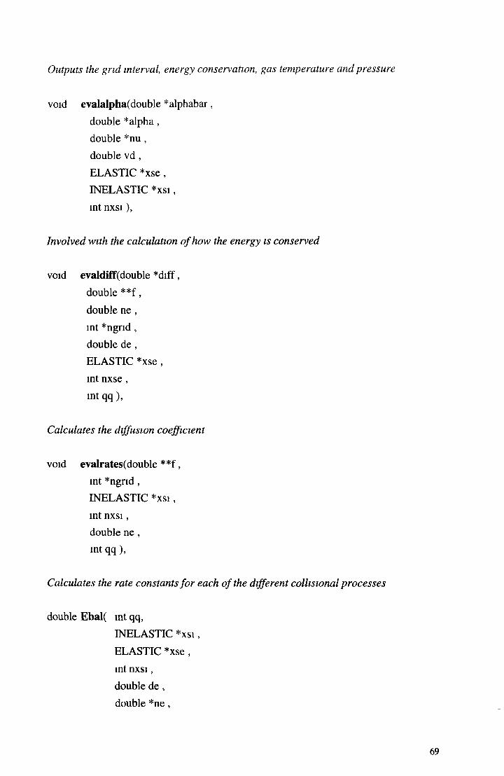
Outputs the grid interval, energy conservation, gas tem perature and pressure

void evaIalpha(double *alphabar,

double * a lpha ,

double *nu ,

double v d ,

ELASTIC *xse ,

INELASTIC * x s i ,

int nxsi ),

Involved w ith the calculation o f how the energy is conserved

void evaldiff(double * d iff ,

double * * f ,

double n e ,

int * n g n d ,

double de ,

ELASTIC *xse ,

int n x s e ,

mt qq ),

Calculates the d iffusion coeffic ien t

void evaIrates(double * * f ,

int * n g n d ,

INELASTIC * x s i ,

int n x s i ,

double ne ,

int qq ),

Calculates the rate constants f o r each o f the d ifferen t co llisional p rocesses

double Ebal( int qq,

INELASTIC * x s i ,

ELASTIC * x s e ,

mt n x s i ,

double d e ,

double * n e ,

double * e f ,

double * e in e l,

double * e e l ,

double *eden ,

double * e s ,

double *ebar,

ITERATE *T,

FILL * F ),

C alculates the energy conservation

void Fillc( in tq ,

INELASTIC *xsi,

ELASTIC *xse,

mt nxsi,

double dt,

double de,

FILL *F,

ITERATE *T,

mt f e ),

This calculates the elem ents o f the prob lem m atrix A

void datsort(ELA STIC * x s e ,

int nxse ,

double *density ,

char ** la b e l,

int ns ,

double n ),

Sorts ou t the data, g iving the cross-sections a t equal d istances C alculates the

densities

void Evalab( int q,

ELASTIC *xse,

int nxse,

double n,

double en,

70

double de,

double tg

FILL *F,

ITERATE * T ),

Calculates the trid iagonal elem ents used fo r the prob lem m atrix A

void Evalab_fe( int q,

ELASTIC *xse,

int nxse,

double n,

double en,

double de,

double tg,

FILL *F,

ITERATE *T),

Calculates the trid iagonal elem ents used fo r the prob lem m atrix A , only it g ives the

f ( t ) norm alization prob lem instead o f the n(e)

void wrate(FILE *ou tfile ,

INELASTIC * x s i ,

int n x s i ,

ELASTIC *xse ,

int n x s e ),

O utputs the collisional rates betw een electrons and neutra l ions f o r each o f the

d ifferent excita tions

void rxsfil(FILE *xsfile ,

INELASTIC * x s i ,

int * n x s i ,

ELASTIC * x s e ,

int * n x s e ,

int *ngrid ,

double d e ,

int ltype ,

int q q ),

71

Reads in the collisional cross sections fo r the d ifferent excitations fro m the data file

xs dat, and p laces them into the structures xse and xsi

void xserror(char error_text[] ,

char cross_section_nam e[],

char species_nam e[]),

This fu n c tio n is ca lled in the even t o f an error, shou ld one arise in the m anagem ent o f

the cross section data I t p rin ts an error m essage to the screen

void rxs(FTLE * f ile ,

double e [ ] ,

double xs[] ,

int n p n t,

char la b e l[] ,

char n am e[]) /* Read a number o f paired data points */,

This fu n c tio n is em ployed by rxsfil, to read in a p a ir o f data po in ts fro m the cross

section f i le

void rdatfil(FELE * in file ,

char x sfiln am [],

double *de ,

double * d t ,

double *en ,

double *n ,

double *ne ,

int *ns ,

double d en sity [],

char ** la b e l,

double *tg ,

int * ity p e ,

double * source ,

mt * q q ),

R eads in p la sm a settings fro m the d a ta file b ! 7 dat

72

ITERATE *allocitrn(int n l ,

int nh ),

A llocates m em ory space fo r a po in ter to the structure T

M INIM UM *allocm r(int n l ,

mt nh ),

A lloca tes m em ory space fo r a po in ter to the structure m r

FILL *aIlocF(int n l ,

int n h ),

A lloca tes m em ory space fo r a p o in ter to the structure F

char *fgetlin(char * s tr ,

mt len ,

FILE » f i le ),

E m ployed by the fu n c tio n rxs() to read in a line fro m a data file , o f a g iven length

INELASTIC *allocxsi(int n l ,

mt n h ),

A lloca tes m em ory space fo r a po in ter to the structure x s i

ELASTIC *allocxse(int n l ,

mt n h ),

A lloca tes m em ory space fo r a po in ter to the structure xse

char *cvector(int n ),

N um erica l R ecipe [10] function , which allocates m em ory fo r an array o f characters

o f size n

char **sarray(int n l ,

mt nh ,

73

int length),

N um erical R ecipe [10] function , which allocates m em ory fo r an m atrix o f characters

o f size nh by length

void free_sarray(char * * s ,

int n l ,

mt n h ,

int len g th ),

N um erica l R ecipe [ 10] function , which fr e e s m em ory space a lloca ted by the fu n c tio n

sarray

void spline(double x [ ] ,

double y [ ] ,

int n ,

double yp l ,

double ypn ,

double y 2 [ ] ),

N um erica l R ecipe [10] function , which fo r a " iven m athem atica l table fu n c tio n y(x),

calculates the second order derivative

void xsinterp(double x a [ ] ,

double y a [ ] ,

double y 2 a [ ] ,

int n ,

double x ,

double *y ,

int lty p e ),

In terpolates the cross section data so tha t there is equal distance betw een the

resulting cross sections In terpolation can be linear or cubic

void hidcm p(double * * a ,

int n ,

int *indx ,

- double * d ),

74

N um erical Recipe [10] function , given an mn m atrix a, it replaces a by the LU

decom position o f a rowwise perm uta tion o f itse lf This m ust be used in conjunction

with lubksbQ

void lubksb(double * * a ,

int n ,

int * m d x ,

double b [ ] ),

N um erica l R ecipe [10] function , used a fter the above function , w hich im plem ents

backw ard substitution, and outputs the solution into vector b, w hich is the solution to

the m atrix p rob lem A b = d

void thres(int n ,

mt *yh ,

int * y l ,

int qq ),

This fu n c tio n is used to calculate the energy thresholds f o r the low er level, when the

direct m atrix redefin ition m ethod is employed, as opposed to the G alerkin m ethod

void M atrix( int q ,

int qq ,

int *ngrid

double h ,

double * * * a ),

Fills the prob lem m atrix A fo r the P oisson case

void M inres(double wu,

int 1 ,

int totalwu,

double res,

int mew,

int level,

mt ah2h,

char TypeName[],

75

M INIM UM *m r),

Tests fo r the best m ultigrid perform ance, fro m all cycles and param eters used, with

increasing W U The cycle number, type, V, and level is recorded fo r each W U

void Solve( int q, ITERATE *T, int lud),

O btains the L U D solution to the m atrix problem , pu tting the solution into f soi, inside

structure T

void Set_M odes(int q, ITERATE *T),

Sets the in itia l guess f o r the m ultigrid approxim ation Can only se t m odes in the case

o f the Poisson prob lem as the m athem atical expressions f o r the m odes o f the

Boltzm ann prob lem are unknown

void DoCycIe(int q, char TypeName[], ITERATE *T, M INIM UM *mr),

Places a string TypeN am e[] containing the m acro nam e into the structure T

void A llCycles(int q, double wusum, ITERATE *T, M INIM UM *mr),

Sets up the in itia l residual and guess f o r the problem , and perform s the cycles

dicta ted by the m acros until a g iven num ber o f W U cycles has been perform ed, o r the

convergence criteria has been reached

double Cal_W U(int q, ITERATE *T),

Calculates roughly the num ber o f W U in each o f the cycles, g iven the coarsest grid

the cycle proceeds dow n to

The prototypes in the file Cycles h are given as follows

double N orm ( mt q, ITERATE *T, int NOrM),

N orm alizes the approxim ation, to that o f the LU D solution

76

Calculates the m axim um error elem ent o f the error vector

double Enorm( int q, ITERATE *T, double enorm_0),

U sed to f in d the norm o f the error norm between the norm alized approxim ation and

the LU D solution

double Residual(int q, ITERATE *T, double res_0),

U sed to f in d the residual norm o f residual equation r = Av-f

double Resmax( int q, ITERATE *T, double resmax_0),

C alculates the m axim um residual e lem ent o f the residual vector

void Iterate_RB_R( int start,

mt finish,

ITERATE *itrn,

int q),

Execute a red-black G auss Seidel iteration, which can start o r f in is h a t the specified

po in ts on the g rid

void Iterate_RB_L(int start,

int finish,

ITERATE *itrn,

int q),

Execute a red-black G auss Seidel backw ard iteration, which can start o r f in is h a t the

specified po in ts on the grid

void Iterate_GS_R(mt start,

mt finish,

ITERATE *itrn,

mt q),

double Emax( int q, ITERATE *T, double emax_0),

77

Execute a basic G auss Seidel fo rw a rd iteration, which can start or fin ish a t the

specified po in ts on the grid

void Iterate_G S_L (int start,

int finish,

ITERATE *itrn,

int q),

Execute a basic G auss Seidel backw ard iteration, which can start o r f in is h a t the

specified po in ts on the g rid

void IterateSort(int rbr,

mt rbl,

int gr,

int gl,

ITERATE *itrn,

int adaptive,

int q),

This fu n c tio n is used to m ake iteration calls easier I t controls w eather o r n o t the

iteration is adaptive, and w ill ca ll one o f the above fo u r fu n c tio n s

void Fix_fr(double *fr, int qq),

This fu n c tio n is used to se t how the adaptive iteration w ill behave

void W rite_fpcoarse(int q, ITERATE *T),

W rites the approxim ation and the LU D solution fo r the low er grids to the f i le

fp co a rse da t

void CalcuIate_R_P(ITERATE *T),

Calculates the tw o m atrices R and P used fo r restriction and in terpolation

void Calculate_G alerkin(ITER A TE *T);

78

C alculates A on the lower grids, using the G alerkin method, m ultip lying the m atrices

R A P

void R estrict RA P(int q, ITERATE *T),

Executes the G alerkin m ethod o f restriction, using the m atrix R fo r restriction

void Restrict(int q, ITERATE *T),

Executes d irec t restriction, which can be w eighted or linear, a n d o f type A H o r A 2 H

void Interpolate_R A P(int q, ITERATE *T),

E xecutes G alerkin m ethod o f interpolation, using the m atrix P fo r in terpolation

void Interpolate(int q, ITERATE *T),

Executes a d irec t interpolation

void Vcycle(int q, int 1 , ITERATE *T),

Executes a Vcycle, descending dow n to the specified level

void F M cycle lA (in t q, int 1 , ITERATE *T),

Executes a FM cycle, o f type 1A

void F M cycle lB (in t q, int 1, ITERATE *T),

E xecutes a FM cycle, o f type IB

void FM cycle2A (int q, int 1 , ITERATE *T),

E xecutes a FM cycle, o f type 2A

void FM cycle2B (in t q, int 1 , ITERATE *T),

E xecutes a F M cycle, o f type 2B

void C C C lcycle(in t q, int 1 , ITERATE *T),

Executes a C C C ¡cycle (defined in appendix C)

void CV C cycle(int q, int 1 , ITERATE *T),

Executes a CVCcycle, (defined in appendix C)

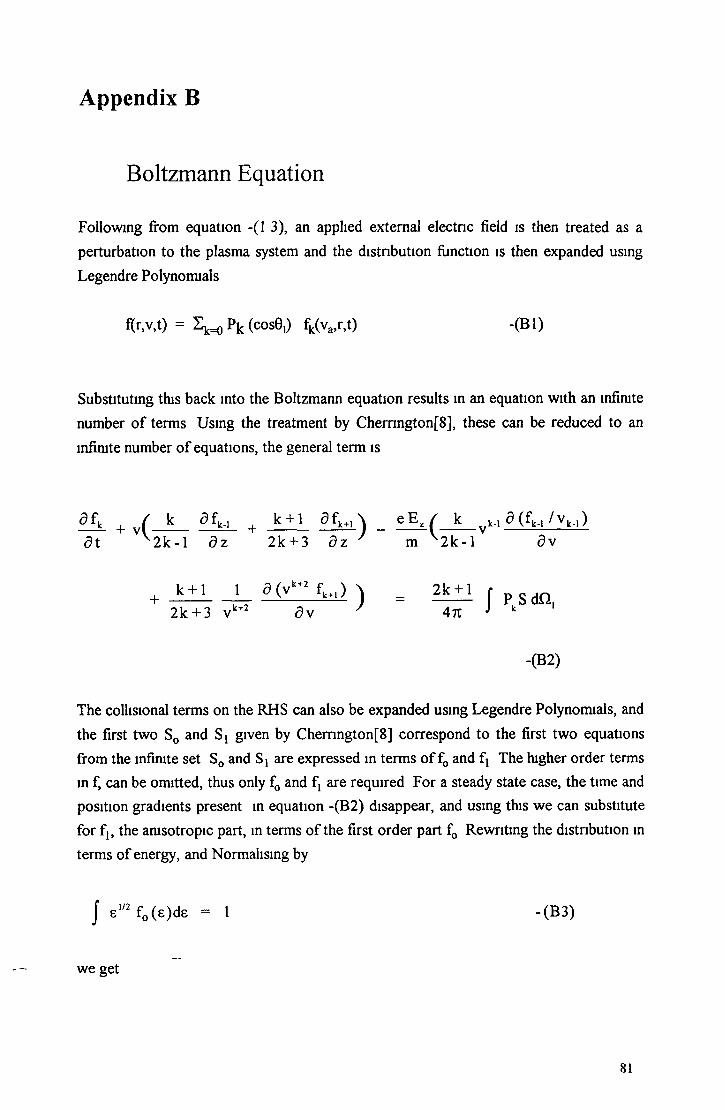
Appendix B

Boltzmann Equation

Following from equation -(1 3), an applied external electric field is then treated as a

perturbation to the plasma system and the distribution function is then expanded using

Legendre Polynomials

f(r,v,t) - I k=0 Pk (cos0,) fk(va,r,t) - (B l)

Substituting this back into the Boltzmann equation results in an equation with an infinite

number o f terms Using the treatment by Chem ngton[8], these can be reduced to an

infinite number o f equations, the general term is

d f k + ( k d f k.i + k + 1 d f k+1 \ _ e E / k ^k.t d ( f k., / v k.,) a t 2 k - l d z 2k + 3 d z ' m ^ 2 k - l d v

k + 1 1 S ( v k+2fk+1) \ _ 2 k + 1) = J Pksdn,J Att J k2k + 3 v k+2 d v ' 471

■(B2)

The collisional terms on the RHS can also be expanded using Legendre Polynomials, and

the first two S0 and S t given by Cherrington[8] correspond to the first tw o equations

from the infinite set S0 and S t are expressed in terms o f f0 and f\ The higher order terms

in f, can be omitted, thus only f0 and fj are required For a steady state case, the time and

position gradients present in equation -(B 2) disappear, and using this w e can substitute

for f b the anisotropic part, in terms o f the first order part f0 Rewriting the distribution in

terms o f energy, and Normalising by

w e get

| e 1,2 f0(e)de = 1 -(B3)

81

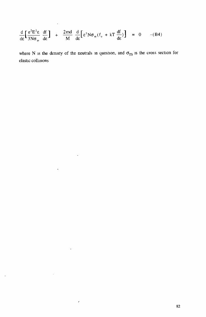
d f e 2E 2e df 1 2m d d f 2xt df 1+ ""m ” de + de * ° - <B4>

where N is the density o f the neutrals in question, and a m is the cross section for

elastic collisions

82

Appendix C

Multigrid Parameters or Settings

The following gives a list o f all the different possible settings, the macros in the

program that correspond to these, and also the different cycles

1) Whether the function Restnct() was weighted This is the averaging o f a given point

to be restricted with its surrounding points, as possible from the C function Restnct()

In this case it is either full weighted as given by equation -(2 40)

e * = l/4( vV , + 2vh21 + vh2l+1) 0 < i < N/2

or linear restriction involving no weighting or averaging o f surrounding points

e2h _ 0 < i < n /2

2) Weather Restrict(AH) or (2AH ) was used, the difference between these is apparent

when calculating the residual r2h from rh There are two possible approaches

AH is used to refer to the following

r2h = Restrict(rh = f 1 - Ahvh) = I ^ f * 1 - Ahvh)

where (f*1 - Ahvh) is calculated first and then the result is restricted to the lower grid

2h

A2H is used to refer to when the restrict operator Ih2h works inside the brackets as

follow s, and operates on the equation before rh is calculated

r2h = Restrict(rh = f 1 - Ahvh) = Ih2h(fh - Ahvh) = - Ih2hAhvh= ph - A2hv2h

3) How low the cycle would progress to or what level the particular cycle would stop

at before proceeding back up to finer grids This is referred to as the 'level'

4) The number o f iterations v performed on each grid

83

5) The definition for the problem matrix A, can be given by either the direct approach,

or the Galerkin method The direct approach involves redefining the matrix A at each

level for that given number of grid points, but with a different energy interval The

Galerkin method calculates A on the lower grids by the expression R A P given in

chapter 2 by the equations -(2 43,44 ,45) The program uses the macro RAP to decide

which o f these two methods it will use If the macro is true, then the Galerkin method

is used, if false, the direct approach

6) The type o f multigrid cycle used, e g Vcycle or FM cycle The program uses a

choice o f eight different cycles, and one o f which is just m onognd Gauss-Seidel

iterations, to which the others can be compared to The program tests the C macro for

each cycle to see whether it is to proceed with that option o f cycle The C functions for

the different cycles are given in the appendix A There are eight different cycles, A-H

The cycles and their corresponding C macros are given

A) The Vcycle, which is executed by the C function Vcycle(), has the macro

VCYCLE This cycle is the most basic fundamental o f all the multigrid cycles

B) A full mulitgnd cycle o f type 1 A, given by the C function FM cycle 1A(), is tested by

the macro FMCYCLE 1A This is first o f four different possible ways to define a full

multigrid cycle As suggested initially by Brandt [3,4,5,6], this cycle could start by

restricting down to the low est grid, without iterating on the way down It uses the fact

that a better guess can more easily found on the coarsest grid, and thus the multigrid

frequency removal mechanism need only start on this grid It was defined that for type

1A, when the cycle reaches the finest grid for the first time, no more Vcycles are

performed This is the cheapest o f all four full multigrid types

C) A full multigrid cycle o f type IB, given by FM cyclelB (), and tested by the macro

FM CYCLE1B This is the same as type 1A only that iterations are performed initially

on descending down from the fine grid to the coarsest, at the start o f the cycle The

rest o f the cycle remains the same

D ) A full multigrid cycle o f type 2A, given by FM cycle2A(), and tested by the macro

FM CYCLE2A This is the same as type 1A only that when the cycle reaches the fine

grid, an extra V cycle() is executed

E) A full multigrid cycle o f type 2B , given by FM cycle2B(), and tested by the macro

FM CYCLE2B This is the same as type IB only in that when the cycle reaches the fine

84

grid, an extra Vcycle() is executed (as like 2A) This is the most costly type, and as it

turns out, any improved performance o f this type will not warrant the extra

computational cost

F) The W cycle is given by W cycle(), and tested by the macro WCYCLE

G) The cycle CCC1 consists o f Vcycles, but after any given number o f Vcycles,

another Vcycle can be executed except the level to which the Vcycle progresses is

different to the rest o f the Vcycles This cycle is given by the C function C C C lcycle(),

and is tested by the macro CCC1

H) The cycle CVC consists o f two separate cycles, one after the other In the simplest

case, both could be Vcycles, but the levels that the two Vcycles descend down to

within the one CVC cycle differs This cycle is given by CVCcycle(), and tested by the

macro CVC

Program Details

The program has 5 structures, xse defined as type ELASTIC, which provides storage

for elastic cross section data, xsi defined as type INELASTIC, which holds inelastic

cross section data The structure T holds the multignd problem itself, A f = frhs’ the

solution fsol> the matrices R and P for Galerkin Restriction and Interpolation, and

multignd parameters, most o f which are set by the Macros at the start o f the program

The structure mr defined as type M INIM UM , holds the parameters which the function

Minres() tests to obtain the best results (low est fractional residual) The structure F

defined as type FILL contains the elements a and b that are produced by the function

Evalab() or Evalab_fe These elements are then placed in the problem matrix A by

Fillc() The parameter list o f most functions in the program was reduced by placing as

much o f the data as possible into structures, which simplified the function calls

dramatically Also, pointers to the structures were passed in the function calls which

enabled any o f the contents in the structure to be altered by the function m question

All functions beginning with a capital letter are either new or have been completely

altered from the original code

85

I

All file pointers apart from infile, and outfile, begin with fp, and are identical in name

to the output files only that the output files contain the extension dat A list of output

files and their purpose is given in appendix A

Program Flow

Diagram -(C l) shows a simple flow, where the main program is split up into 7 blocks,

each of which is numbered

1

-(C l)

86

The source code for the main program is given in Multignd_Study c The source file

Cycles c contains the algorithms for all the cycles The prototypes for these are both

given in the appendix A The flow of the main program Multigrid_Study c is now

discussed

Once the variable types and the five structures in main have been declared, main then

opens the first data file (block 1), called b l7 dat The function rdatfil() then reads some

plasma parameters, the most important being the size q, giving 2q- l internal grid

points

Memory is then allocated for the structures (block 2) xsi, xse, T, mr and F This is

done by allocating a one dimensional array for each o f the structures For the

structures T, mr and F, an array o f size one is allocated The reason an array of

structures was allocated instead o f just a structure is to enable the contents o f all these

structures to be manipulated more easily by any functions which use them Allocating

an array o f structures offers easier notation in the function call than the other option of

using a pointer to each structure in the function call, although this is a matter o f

preference

All functions beginning with Alloc, are associated with memory allocation The

functions Alloc_T(), Alloc_mr(), and Alloc_F actually allocate the memory for the

contents inside each individual structure The contents o f the xsi and xse structures is

allocated when needed in the different functions as required later The function

Set_T_F_mr() then fills or sets the arrays and values o f the contents o f the three

structures

Input from the second file xs dat is then read by block 3 The function rxsfil() among

other things reads the cross-sections from the data file xs dat into the tw o structures

xse (elastic cross-sections) and xsi (inelastic) The function datsort() then alters the

number and spacing o f the cross-sections in energy such that there are cross-sections

given for each energy point on the grid The function also performs manipulations on

the densities with a view to obtaining the specific mass ratios for each o f the different

species and states present in the plasma, which are required for equation -(1 9)

Block 4 then proceeds to fill the contents o f the problem matrix A , and also sets the

boundary conditions, by assigning a value for the first element on the right hand side,

as equation -(1 9) There is a simple 'if switch, testing as to what type o f lower grid

matrix redefinition is used, e g the Galerkin method (using full the operator matrices R

87

and P) tested by the macro RAP. If RAP is not true (has a value of zero) then the

second option of direct matrix redefinition for each level is then used. For every level q

down to 1, the problem matrix A is defined. If the RAP is true, then A is found only

for the fine grid, and the function Calculate_R_P() proceeds to find the matrices P and

R for each level, and when calculated calls the function Calculate_Galerkin() which

then calculates RAP for each level. The matrices for R and P are found in accordance

to Briggs [7]. R has N/2 -1 rows and N-l columns, given N-l internal grid points in

the system. P has N-l rows and N/2 -1 columns.

Block 4 tests for the option of either a Boltzmann problem or Poisson, and also gives

the option (by testing the macro GAUSS_JORDON) to calculate the eigenvalues of

the problem matrix A using the function Eigen(), which employs the C Numerical

Recipes functions [10] gaussj(), elmhs() and hqr().

If the option of Boltzmann is chosen, the function Evalab() calculates the values for the

coefficients a and b in equation -(1.9a). These are stored in the structure F (of type

FILL). The function Fillc(), then uses these diagonal coefficients along with the cross-

sections and other parameters to calculate and fill all the elements in the problem

matrix A. As mentioned, there are two possible normalisations, one solving for n(e)

and the other f(e). The function Evalab() and Fill(„,0) correspond to the first, n(e),

where the last argument 0 that Fill() takes sets the function to the n(e) option. If the

f(£) normalisation is required, the function Evalab() is replaced by Evalab_fe(), and the

last argument of Fill() becomes 1 to give Fill(,„l).

If the Poisson option is taken, the function Matrix() calculates and fills the problem

matrix A.

At the end of block 4, the system is now defined, all input information has been

assimilated, and the multigrid aspect takes over.

The function Solve() at the start of block 5 obtains the LUD solution to the defined problem, and stores this separately from the multi grid solution. A results file is then set

by Set_fpcycle(), which will record the performance of each different case scenario.

This is then opened and left open for the duration of each case in block 5. A series of

nested for loops is used to sweep through all the options. In the outer loop

Set_Wexecute() sets the number of times this 'for' loop is repeated, depending on the two macros LINEAR and WEIGHT. These give the option of weighted restriction or

linear (or both). Similarly, Set_Aexecute() sets the number of times the next 'for' loop

88

is repeated, depending on the two macros AH and A2H, which correspond to the type

of restriction discussed earlier The function Set_W eights() then sets the multigrid

parameters inside the structure T, to either linear, weighted or both Similarly

Set_Restrict() sets the type o f restriction in the multigrid structure T These functions

were written to reduce the size o f the function main() in M ultignd_Study c

They enable all the different cycles and multigrid parameters to be attempted on the

same set problem, so that the file fpcycle dat can contain all results from each different

case This file could be used to compare the results, and plot any case against another

This was the approach taken to observe multigrid performance (e g by

experimentation)

All functions beginning with Write, are new functions writing to files associated with

the multigrid performances Those beginning with w, are original existing functions

which have been manipulated, which output the plasma properties to the results file

b l7 res

Code Testing of the Fourier Function

The Fourier() function which obtains the sine fourier transform o f a 1 x N - l vector,

using the Numerical Recipes [10] function sineft(), has been tested by using the

coincidence that the eigen functions or eigen modes o f the Poisson problem are in fact

sine waves between the tw o end boundary points Thus by setting up the Poisson

problem, solving it, then adding a particular eigen mode, which becomes the error, it is

possible to treat this as an initial guess A sine fourier transform o f the error should

reveal that frequency mode If all modes are present in equal amounts, then the fourier

transform o f the error is a horizontal line

89

Appendix D

Boltzmann Normalization

Equation -(1 9) gives the Boltzmann problem for the normalization n(e), which describes

the number o f electrons in the plasma at energy s, and is given by

J n ( s ) de = ne - ( D l )

where ne is the number o f electrons in the plasma However, given the relation between

fl e) and n(e) as

n(e) = f(e) e1/2 rig -(D2)

then

J 81/2 f(e) ds = 1 - ( D 3)

Using the above equations w e can now rewrite the Boltzmann problem given by equation

-(1 9) as,

= Ck-,fk-l + gk+1fk+! -(Ck + gk)fk + ZN» [Rsjk.m As'/2k'/2 f k+m,_ + R*Ijk. » A 1/îkl/ï fk %N N sdm dt

+ R ' A s1/2k ‘'2 fk+m. + 8 ik Z R ‘sinA e1/2k U2 f m- ( R sjlt + R-Sjk + R ,lk)AE1'2k 1/î f j

-(D 4)

where a, and b from equation -(1 9) become c, and g respectively, using the above

relations, and also equations -(1 9a,b,c) W e can define c, and g (which correspond to a

and b) as follows

90

3m W v; / VA e ^ “ ' 4 ' ~ ‘ ' 2 A e v T ~ 6‘ T ^ T/ N

2 N £ ( E y J _ / J _ \ / Ae j y / 2 ^ , / 2 . vk ( + KT 2KT \ V2 l/2gk 3m V 4 (k 1} > * * + Ek + Ae k

XN

2NeV E y 1 / I

-(D4a)

where e ;= k A e , e k = e ;., -(D4b)

W = ( v ) l'2? q-,J‘t ó ) ■ ■

-(D4c)

Equation -(D4b and c) remain the same

91

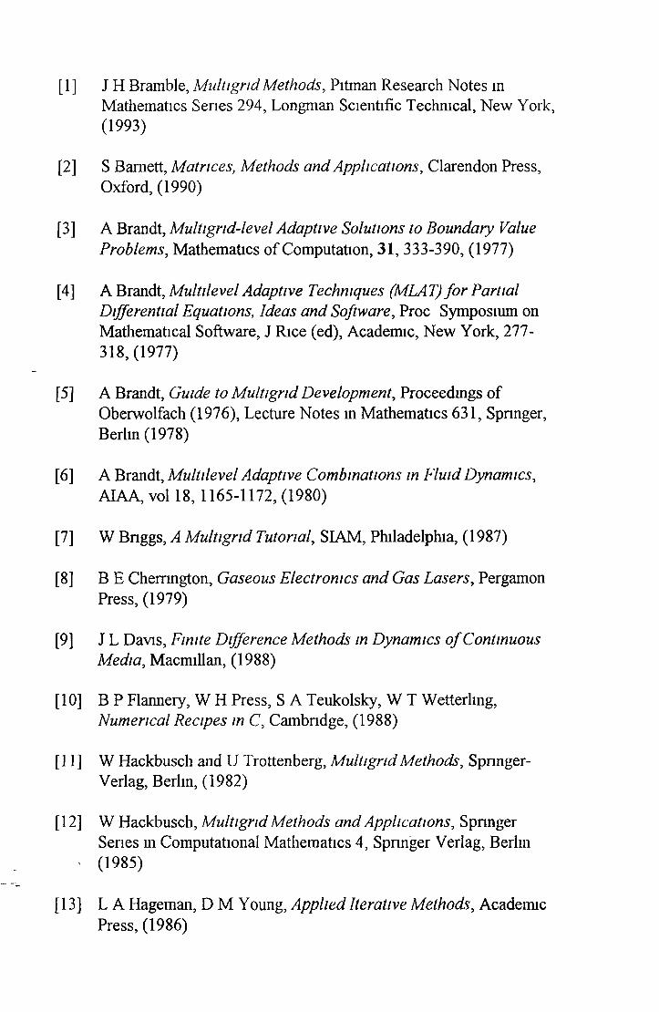
[1 ] J H Bramble, Mult ¡grid Methods, Pitman Research Notes inMathematics Series 294, Longman Scientific Technical, New York, (1993)

[2] S Barnett, Matrices, Methods and Applications, Clarendon Press, Oxford, (1990)

[3] A Brandt, Multigrid-level Adaptive Solutions to Boundary Value Problems, Mathematics of Computation, 31, 333-390, (1977)

[4] A Brandt, Multilevel Adaptive Techniques (MLAT) fo r Partial Differential Equations, Ideas and Software, Proc Symposium on Mathematical Software, J Rice (ed), Academic, New York, 277- 318,(1977)

[5] A Brandt, Guide to Multigrid Development, Proceedmgs of Oberwolfach (1976), Lecture Notes in Mathematics 631, Spnnger, Berlin (1978)

[6] A Brandt, Multilevel Adaptive Combinations in Fluid Dynamics, AIAA, vol 18, 1165-1172,(1980)

[7] W Bnggs, A Multigrid Tutorial, SIAM, Philadelphia, (1987)

[8] B E Chemngton, Gaseous Electronics and Gas Lasers, Pergamon Press, (1979)

[9] J L Davis, Finite Difference Methods in Dynamics o f Continuous Media, Macmillan, (1988)

[10] B P Flannery, W H Press, S A Teukolsky, W T Wetterlmg, Numerical Recipes in C, Cambridge, (1988)

[11] W Hackbusch and U Trottenberg, Multigrid Methods, Sprmger- Verlag, Berlin, (1982)

[12] W Hackbusch, Multigrid Methods and Applications, Spnnger Series m Computational Mathematics 4, Spnnger Verlag, Berlin

• (1985)

[13] L A Hageman, D M Young, Applied Iterative Methods, Academic Press, (1986)

[14] P W Hemker, P Wesselmg, MultigridMethods IV, ISNM, vol 116, Proceedings of the 4th European Multigrid Conference,Amsterdam, Birkhauser-Verlag, (1993)

[15] T Holstem, Energy Distribution o f Electrons in High Frequency Gas Discharges, Phys Rev 70,367-384,(1946)

[16] J J Lowke, A V Phelps, and B W Irwin, Predicted Electron Transport Coefficients and Operating Characteristics o f C02- N2He Laser Mixtures, J Appl Phys 44,4664-4671

[17] S McCormick, Multigrid Methods, vol 3, SIAM Frontier Senes, SIAM, Philadelphia, (1987)

[18] S McCormick, Multigrid Methods, Frontiers m Applied Mathematics, SIAM, Philadelphia, (1987)

[19] S McCormick, Multigrid Methods, vol 110, Marcel Dekker, me, (1987)

[20] S McCormick, Multilevel Adaptive Methods fo r Partial Differential Equations, SIAM Frontier in Applied Mathematics 6, Philadelphia, (1989)

[21] S D Rockwood, Elastic and Inelastic Cross Sections fo r Electron- Hg Scattering from Hg Transport Data, Phys Rev A 8, 2348, (1973)

[22] K A Stroud, Further Engineering Mathematics, 2nd ed, Macmillon Education Ltd, (1990)

[23] P Wesselmg, An Introduction to Multigrid Methods, Wiley Intemation Science, (1992)