2103946 (1 of 17) © 2021 Wiley-VCH GmbH

www.advmat.de

ReseaRch aRticle

Fundamental Limits to the Refractive Index of Transparent Optical Materials

Hyungki Shim, Francesco Monticone, and Owen D. Miller*

H. Shim, O. D. MillerDepartment of Applied Physics and Energy Sciences InstituteYale UniversityNew Haven, CT 06511, USAE-mail: owen.miller@yale.eduH. ShimDepartment of PhysicsYale UniversityNew Haven, CT 06511, USAF. MonticoneSchool of Electrical and Computer EngineeringCornell UniversityIthaca, NY 14853, USA

The ORCID identification number(s) for the author(s) of this article can be found under https://doi.org/10.1002/adma.202103946.

DOI: 10.1002/adma.202103946

rule, are surprisingly strong constraints on refractive-index lineshapes, imposing strict limitations to refractive index at high frequency, with only weak (cube-root) increases possible through electron-density enhancements or large allowable dispersion. We show that a large range of questions around maximum index, including bandwidth averaged objectives with constraints on dispersion and/or loss, over the entire range of causality-allowed refractive indices, can be formulated as linear programs amenable to computa-tional global bounds, and that many ques-tions of interest have global bounds with optima that are single Drude–Lorentz oscillators, leading to simple analytical bounds. For the central question of max-imum index at any given frequency, we show that many natural materials already closely approach the Pareto frontier of tradeoffs with density, dispersion, and frequency, with little room (ranging from

1.1–1.5×) for significant improvement. We apply our frame-work to high-index optical glasses (characterized by their Abbe number) and bandwidth-based bounds. For anisotropic refrac-tive indices, or materials with magnetic in addition to electric response, we use a nonlocal-medium-based transformation to prove that any positive- or negative-semidefinite material properties cannot surpass these bounds, although there is an intriguing loophole for hyperbolic metamaterials. At optical fre-quencies, there are few or no natural materials with high index and high dispersion, but we show that composite metamate-rials can be designed to have refractive indices approaching our bounds. With conventional metals such as gold and aluminum, we show that low-loss refractive indices of 5 in the visible, 18 in the near-infrared (3 μm wavelength), and 40 in the mid-infrared (10 μm wavelength) are achievable. If a near-zero-loss metal can be discovered or synthesized,[15,16] high-dispersion refractive indices above 100 would be possible at any optical frequency.

A large material refractive index n offers significant benefits for nanophotonics devices. First, the reduced internal wave-length enables rapid phase oscillations, which enable wavefront reshaping over short distances and is the critical requirement of high-efficiency metalenses and metasurfaces.[1–5,7,17] Second, it dramatically increases the internal photon density of states, which scales as n3 in a bulk material[18] and offers the possibility for greater tunability and functionality. The enhanced density of states is responsible for the ray-optical 4n2 “Yablonovitch limit” to all-angle solar absorption[19] and the random surface textures

Increasing the refractive index available for optical and nanophotonic sys-tems opens new vistas for design, for applications ranging from broadband metalenses to ultrathin photovoltaics to high-quality-factor resonators. In this work, fundamental limits to the refractive index of any material are derived, given only the underlying electron density and either the maximum allow-able dispersion or the minimum bandwidth of interest. In the realm of small to modest dispersion, the bounds are closely approached and not surpassed by a wide range of natural materials, showing that nature has already nearly reached a Pareto frontier for refractive index and dispersion. Conversely, for narrow-bandwidth applications, nature does not provide the highly disper-sive, high-index materials that the bounds suggest should be possible. The theory of composites to identify metal-based metamaterials that can exhibit small losses and sizeable increases in refractive index over the cur-rent best materials is used. Moreover, if the “elusive lossless metal” can be synthesized, it is shown that it would enable arbitrarily high refractive index in the high-dispersion regime, nearly achieving the bounds even at refractive indices of 100 and beyond at optical frequencies.

1. Introduction

Increasing the refractive index of optical materials would unlock new levels of functionality in fields ranging from metasurface optics[1–7] to high-quality-factor resonators.[8–14] In this article, we identify fundamental limits to the maximum possible refractive index in any material or metamaterial, dependent only on the achievable electron density, the fre-quency range of interest, and possibly a maximum allowable dispersion. We show that the Kramers–Kronig relations for optical susceptibilities, in conjunction with a well-known sum

Adv. Mater. 2021, 2103946

© 2021 Wiley-VCH GmbH2103946 (2 of 17)

www.advmat.dewww.advancedsciencenews.com

employed in commercial photovoltaics. Third, high optical index unlocks the capability for near-degenerate electric and magnetic resonances within nano-resonators. Tandem electric and magnetic response is critical for highly directional control of waves; whereas a single electric dipole radiates equally into opposite directions, a tandem electric and magnetic dipole can radiate efficiently into a single, controllable direction, known as the “Kerker effect”,[20] then forming the building blocks of complex, tailored scattering profiles.[21–29] Bound states in the continuum utilize Kerker-like phenomena and may also ben-efit from high index.[30] Fourth, a large phase index can lead to a large group index, which underpins the entire field of slow light,[31,32] for applications from delay lines to compressing optical signals. Finally, high refractive index enables significant reductions of the smallest possible mode volume in a dielec-tric resonator. Recent theoretical and experimental demonstra-tions show the possibility for highly subwavelength mode vol-umes in lossless dielectric materials.[33–37] In this case, a high refractive index increases the discontinuities in the electric and displacement fields across small-feature boundaries, ena-bling significant enhancements of the local field intensity that are useful for applications from single-molecule imaging[38–41] to high-efficiency nonlinear frequency conversion.[42–45] For any application, engineering tradeoffs (ease of synthesis, fab-rication-error sensitivity, etc.) come into play when selecting which material to use at a given moment in time, but from the perspective of photonic design and reaching for the limits to what is possible, increasing refractive index is almost always beneficial.[46,47]

The very highest refractive indices of transparent natural materials are 4 to 4.2 at near-infrared frequencies,[48] and 2.85 at visible frequencies.[49] Metamaterials, comprising multiple materials combined in random or designed patterns, have been designed with refractive indices up to 5 at visible frequen-cies,[50] albeit with significant material losses. As the frequency is reduced, the refractive index can be significantly increased, a feature predicted by our bounds and borne out by the literature. Low-loss metamaterials have been designed to achieve refractive indices near 7 at infrared frequencies (3–6 μm wavelengths)[51] and above 38 at terahertz frequencies.[52] Near the phase tran-sition of ferroelectric materials, it is known (Chapter  16 of ref.  [53]) that in principle the refractive index is unlimited. Yet the caveat is that the frequency at which this occurs must go to zero. Experimental and theoretical studies have identified multiple materials with “colossal” zero-frequency (electrostatic) dielectric constants,[54] even surpassing values of 10 000.[55] All of these results are consistent with and predicted by the bounds that we derive.

Recently, scattering measurements on the perovskite mate-rial KTN:Li near its phase transition led to the claim of a refractive index of at least 26 across the entire visible region.[56] As we discuss further below, such a refractive index appears to be theoretically impossible: it would require an electron density and/or dispersion almost three orders of magnitude larger than those of known materials, an unprecedented anomaly. Thus our work suggests that the experimental measurements may arise from linear-diffraction or even non-linear optical effects, and do not represent a true phase-delay refractive index.

Theoretical inquiries into possible refractive indices have revolved around models that relate refractive index to other material properties, and particularly that of the energy gap in a semiconducting or insulating material. The well-known Moss relation[57,58] is a heuristic model that suggests that refractive index falls off as the fourth root of the energy gap of the mate-rial. This model can effectively describe some materials over a limited energy range, but is not a rigorous relation and cannot be used for definite bounds. Another approach, related to ours, is to use the Kramers–Kronig relation for refractive index to suggest that refractive index should scale with the square root of electron density.[59,60] But this approach has not been used for definite bounds, nor is the scaling relation correct: as we show, an alternative susceptibility-based sum rule shows that the refractive index should scale as the cube-root of electron density (for a fixed dispersion value, without which refractive index can in principle be arbitrarily high). A recent result uti-lizes renormalization-group theory to suggest that the refrac-tive index of an ensemble of atoms must saturate around 1.7 (ref.  [60]). There have also been bounds on nonlinear suscep-tibilities using quantum-mechanical sum rules,[61,62] but, as far as we know, there have not been bounds for arbitrary materials on linear refractive index, which is the key controlling property for optics and nanophotonics applications.

Separately, bounds have been developed for other material properties, such as the minimum dispersion of a negative-per-mittivity or negative-index material.[63,64] Such bounds utilize causality properties, similar to our work, to optimize over all possible susceptibility functions. There have also been claims of bounds on the minimum losses of a negative-refraction material,[65] though recent work[66] has identified errors in that reasoning and shown that lossless negative-refraction materials are, in principle, possible. If the approaches of these papers were directly applied to refractive index, they would yield trivi-ally infinite bounds, as they do not make use of the electron-density sum rule of Equation  (2) below. A large range of elec-tromagnetic response functions have recently been bounded through analytical or computational approaches,[46,47,67–77] but none of these approaches have been applied to refractive index, nor is there a clear pathway to do so.

In this paper, we establish the maximal attainable refrac-tive index for arbitrary passive, linear, bianisotropic media, applicable to naturally occurring materials as well as artifi-cial metamaterials. We first derive a general representation of optical susceptibility starting from the Kramers–Kronig rela-tions (Section  2), enabling us to describe any material by a sum of Drude–Lorentz oscillators with infinitesimal loss rates. By considering a design space of an arbitrarily large number of oscillators, the susceptibility is a linear function of the degrees of freedom, which are the oscillator strengths. Many constraints (dispersion, bandwidth, loss rate, etc.) are also linear functions of the oscillator strengths, which themselves are constrained by the electron density via a well-known sum rule. Thus a large set of questions around maximum refrac-tive index are linear programs, whose global optima can be computed quickly and efficiently.[78] The canonical question is: what is the largest possible refractive index at any frequency ω, such that the material dispersion is bounded? In Section 3 we show that this linear program has an analytical bound, which

Adv. Mater. 2021, 2103946

© 2021 Wiley-VCH GmbH2103946 (3 of 17)

www.advmat.dewww.advancedsciencenews.com

is a single, lossless Drude–Lorentz oscillator (corresponding to all oscillator strengths being concentrated at a single electronic transition). These bounds describe universal tradeoffs between refractive index, dispersion, and frequency, and we show that many natural materials and metamaterials closely approach the bounds. We then devote a separate section (Section 4) to optical glasses, which are highly studied and critical for high-quality optical components. We show that our bounds closely describe the behavior of such glasses, and that there may be opportu-nities for improvement at low Abbe numbers (high dispersion values). An alternative characterization for refractive index may not be a specific dispersion value, and instead a desired band-width of operation, and in Section 5 we derive bounds on refrac-tive index as a function of allowable bandwidth. Across all of our bounds we find that there may be small improvements pos-sible relative to current materials (1.1–1.5×). Finally, we consider the possibilities of anisotropy, magnetic permeability, and/or magneto-electric coupling in Section  6. We show that a large swath of such effects cannot lead to higher refractive indices, and are subject to the same isotropic-index bounds derived ear-lier in the paper. We also find intriguing loopholes including gyrotropic plasmonic media (which have a modified Kramers–Kronig relation) and hyperbolic metamaterials, although the former may be particularly hard to achieve at optical frequen-cies while the high-index modes in the latter may be difficult to access for free-space propagating plane waves. We identify exactly the material properties that enable such loopholes. Furthermore, we use the theory of composites to design low loss, highly dispersive, metal-based metamaterials with higher indices than have ever been measured or designed (Section 7). In the Conclusion, Section 8, we discuss possible extensions of our framework to incorporate alternative metrics, gain media, anomalous dispersion, and nonlinear response.

2. Maximum Refractive Index as a Linear ProgramTo identify the maximal refractive index, one first needs a rep-resentation of all physically allowable material susceptibilities. We consider here a transparent, isotropic, nonmagnetic mate-rial, which can be described by its refractive index n, relative permittivity ε = n2, or its susceptibility χ  = ε − 1. (We discuss extensions to anisotropic and/or magnetic materials in Sec-tion  6 and we discuss the possible inclusion of loss below.) Instead of assuming a particular form for the susceptibilities (like a small number of Drude–Lorentz oscillators), we assume only passivity: that the polarization currents in the material do no net work. Any passive material must be causal;[79] causality, alongside technical conditions on the appropriate behavior at infinitely large frequencies on the real axis, implies that each of the material parameters must satisfy the Kramers–Kronig (KK) relations. One version of the KK relation for the material susceptibility relates its real part at one frequency to a principal-value integral of its imaginary part over all frequencies:[80]

Re ( )2 Im ( )

d0

2 2∫χ ωπ

ω χ ωω ω

ω= ′ ′′ −

′∞

(1)

Any isotropic material’s susceptibility must satisfy Equation (1). The existence of KK relations, together with passivity restric-tions, already imply bounds on minimum dispersion in regions of negative refractive index,[63–65] but it does not by itself impose any bound on how large the real part of the susceptibility (and correspondingly the refractive index) can be. The key constraint is the “f-sum rule:” a certain integral of the imaginary part of the susceptibility must equal a particular constant multiplied by the electron density Ne of the medium. Typically, electron density is folded into a frequency ωp, which for metals is the plasma frequency but for any material describes the high-fre-quency asymptotic response of the material. The f-sum rule for the susceptibility is[80–83]

e N

mIm ( ) d

2 20

2e

0 e

p2

∫ω χ ω ω πε

πω′ ′ ′ = =

∞

(2)

where e is the charge of an electron, ε0 the free-space permit-tivity, and me the electron rest mass. This sum rule arises as an application of the KK relation of Equation  (1): at high enough frequencies ω, the material must be nearly transparent, with only a perturbative term that arises from the individual elec-trons without any multiple-scattering effects. The sum rule of Equation  (2) is the critical constraint on refractive index: intuitively, it places a limit on the distribution of oscillators in any material; mathematically, it limits the distribution of the measure Im ( )dω χ ω ω′ ′ ′ that appears in Equation (1).

To simulate any possible material, we must discretize Equations (1) and (2) in a finite-dimensional basis. If we use a finite number N of localized basis functions (e.g., a colloca-tion scheme[84] of delta functions), straightforward insertion of the basis functions into Equation (2), in tandem with the con-straint of Equation  (1), leads to a simple representation of the susceptibility:

c

i

Ni

i

Re ( )1

p2

2 2∑χ ωω

ω ω=

−=

(3)

1ci

i∑ = (4)

Equation  (3) distills the Kramers–Kronig relation to a set of “lossless” Drude–Lorentz oscillators with transition frequencies ωi and relative weights, or oscillator strengths, ci. Equation (4) is a renormalized version of the f-sum rule of Equation (2), thanks to the inclusion of p

2ω in the numerator of Equation (3). There is one more important restriction on the ci values: they must all be positive, since Im ( )ω χ ω′ ′ must be positive for a passive material (under an e−iωt time-harmonic convention). Given Equations (3) and (4), it now becomes plausible that there is a bound on refractive index: the oscillators of Equation (3) repre-sent all possible lineshapes, and the sum rule of Equation  (4) restrict the oscillator strengths, and effective plasma frequen-cies, of the constituent oscillators.

It is important to emphasize that the constants in the sum rule of Equation (2) are indeed constants; in particular, that the mass me is the free-electron mass and not an effective mass of an electron quasiparticle. In interband models,[85,86] the linear susceptibility can be written as a sum of Drude–Lorentz oscil-lators similar to Equation  (3) and containing the effective

Adv. Mater. 2021, 2103946

© 2021 Wiley-VCH GmbH2103946 (4 of 17)

www.advmat.dewww.advancedsciencenews.com

masses of the relevant bands. But for those models, the sum over all bands leads to the free-electron mass in the final sum rule.[86] Alternatively, one can use the fact that electrons can be considered as free, non-interacting particles in the high-frequency limit.[87] Thus the only variable in the sum rule is the electron density, which itself does not vary all that much over all relevant materials at standard temperatures and pressures. It is equally important to emphasize that the representation of Equation  (3) does not rely on any of the standard assump-tions of interband models (no many-body effects, periodic lat-tice, etc.), and is valid for any linear (isotropic) susceptibility, assuming only causality. Equation  (3) is not a Drude–Lorentz approximation or model; instead, it is a first-principles repre-sentation of the Kramers–Kronig relations.

To determine the maximum possible refractive index, one could maximize Equation (3) over all possible sets of parameter values for the oscillator strengths and transition frequencies, ci and ωi, respectively. However, a global optimization over the Drude–Lorentz form that is nonlinear in the ωi will be practi-cally infeasible for a large set of transition frequencies. Instead, we a priori fix a very large number of possible oscillator transi-tion frequencies ωi, and then treat only the corresponding oscil-lator strengths ci as the independent degrees of freedom. This “lifting” transforms a moderately large nonlinear problem to a very large linear one, and there are well-developed tools for rap-idly solving for the global optima of linear problems.[78,88]

Crucially, not only is the susceptibility linear in the oscil-lator-strength degrees of freedom ci, but also are many pos-sible quantities of interest for constraints: first-, second-, and any-order frequency derivatives of the susceptibility, loss rates (the imaginary part of the susceptibility), etc. Thus maximizing refractive index over any bandwidth, or collection of frequency points, subject to any constraints over bandwidth or dispersion, naturally leads to generic linear programs of the form:

maximize

subject to 0

1 10

z c

A c b

cc

c

T

jT

j

T

+ ≤=

≥

(5)

where c without a subscript denotes the length-N vector com-prising the oscillator strengths, j indexes any number of pos-sible constraints, the constraint 1Tc = 1 corresponds to the sum rule ∑ici = 1, and z, Ai, and bi are the appropriate vectors and matrices that are determined by the specific objectives, con-straints, and frequencies of interest. There are well-developed tools for rapidly solving for the global optima of linear prob-lems such as Equation  (5), and in the following sections we identify important questions that take this form.

Equation  (5) represents the culmination of our transfor-mation of generic refractive-index-maximization problems to linear programs. A natural question might be why we use the Kramers–Kronig relation, Equation  (1), and sum rule, Equa-tion (2), for material susceptibility χ instead of refractive index n directly? In fact, one could replace all of the preceding equa-tions with their analogous refractive-index counterparts, and arrive at an analogous linear-program formulation for refractive index. But the bounds would be significantly looser, the phys-ical origins for which we explain in Section 3.3. Instead, it turns

out that the susceptibility-based formulation presented above leads to bounds that are rather tight.

3. Single-Frequency Bound

3.1. Fundamental Limit

A canonical version of the refractive-index question is: what is the largest possible refractive index of a transparent (loss-less) medium, at frequency ω, subject to some maximum allowable dispersion? The dispersion constraint is important for many applications, from metalenses to photovoltaics, where one may want to operate over a reasonable bandwidth or minimize the phase- and/or group-velocity variability that can be difficult to overcome purely by design.[89–91] Given the susceptibility representation of Equations (3) and (4) in Sec-tion 2, we can formulate the maximum-refractive-index ques-tion in terms of the susceptibility, and then transform the optimal solution to a bound on refractive index. We assume here a nonmagnetic medium, in which case we can connect electric susceptibility to refractive index; in Section  6 we show that the same bounds apply even in the presence of magnetic response.

The formulation of this canonical single-frequency refrac-tive-index maximization as a linear program is straightfor-ward. The Kramers–Kronig representation of Equation  (3) can be written as χ(ω) = ∑icifi(ω), where fi at frequency ω is given by f i i( ) /( )p

2 2 2ω ω ω ω= − and χ(ω) is linear in the ci values. The dispersion, as measured by the frequency derivative of the real part of the susceptibility, has the same representation but with fi(ω) replaced by its derivative f i i( ) 2 /( )p

2 2 2 2ω ωω ω ω′ = − . Then, the largest possible susceptibility at frequency ω, with disper-sion constrained to be smaller than an application-specific con-stant χ ′, is the solution of the optimization problem:

maximize c f

c f

c c

Re ( ) ( )

subject to dRe ( )d

( )

1, 0

c i

N

i i

i

N

i i

i

N

i i

1

1

1

i∑

∑

∑

χ ω ω

χ ωω

ω χ

=

= ′ ≤ ′

= ≥

=

=

=

(6)

Equation  (6) is of the general linear-program form in Equa-tion (5). Comparing the two expressions, the vector z has fi(ω) as its elements. There is only a single index j, with matrix A1 given by a single column with values ( )f i ω′′ and b1 is a vector of 1’s multiplied by −χ′. To computationally optimize the max-imum-index problem of Equation  (6), one must simply repre-sent a sufficiently large space of possible oscillator frequencies ωi. Since we are interested in transparent (lossless) media, there should not be any oscillator at the frequency of interest ω (oth-erwise there will be significant absorption). Nor should there be any oscillator frequencies ωi < ω, which can only reduce the susceptibility at ω. Thus, one only needs to consider oscillator strengths ωi greater than ω.

Strikingly, for any frequency ω, electron density Ne (or plasma frequency ωp), and allowable dispersion χ′, the optimal solution to Equation  (6) is always represented by a

Adv. Mater. 2021, 2103946

© 2021 Wiley-VCH GmbH2103946 (5 of 17)

www.advmat.dewww.advancedsciencenews.com

single nonzero oscillator, with strength c0  = 1 and frequency

ω ω ω ω χ= + ′1 2 /( )0 p2 3 . We prove in the Supporting Infor-

mation that this single-oscillator solution is globally optimal. The intuition behind the optimality of a single oscillator can be understood from Figure  1. The susceptibility of a single oscillator is governed by three frequencies: the frequency of interest, ω, the oscillator frequency, ω0, and the electron-den-sity-based plasma frequency, ωp. The static susceptibility of such an oscillator at zero frequency is given by /p

2 20χ ω ω= . This

sets a starting point for the susceptibility that ideally should be as large as possible. The plasma frequency is fixed for a given electron density, and thus the only way to increase the static susceptibility is to reduce the oscillator frequency ω0 (as indi-cated by the black left arrow). Yet this comes with a tradeoff: as ω0 decreases, the oscillator nears the frequency of interest, and the dispersion naturally increases. Hence for minimal dis-persion one would want as large of an oscillator frequency as possible. A constraint on allowable dispersion thus imposes a bound on how small of an oscillator frequency one can have, and the maximum refractive index is achieved by concentrating all of the available oscillator strength, determined by the f-sum rule, at that frequency.

The single-oscillator optimality of the solution to Equa-tion  (6) leads to an analytical bound on the maximum achiev-able refractive index. Denoting a maximal refractive-index dis-persion n′ = χ′/2n (from χ = n2 − 1), straightforward algebra (cf. Supporting Information) leads to a general bound on achiev-able refractive index:

n

n

n( 1)2 2p2ωω

−≤

′ (7)

Equation (7) is a key result of our paper, delineating the largest achievable refractive index at any frequency for any passive, linear, isotropic material. Equation (7) highlights the three key determinants of maximum refractive index: electron density, allowable dispersion, and frequency of interest. We will discuss each of these three dependencies in depth. First, though, there is a notable simplification of the refractive-index bound, Equa-tion  (7), when the refractive index is moderately large. In that case, the left-hand side of Equation (7) is simply the cube of n; taking the cube root, we have the high-index (n2 ≫ 1) bound:

nnp

2 1/3ω

ω≤

′

(8)

The cube-root dependence of the high-index bound, Equa-tion  (8) is a strong constraint: it says that increasing electron density or allowable dispersion by even a factor of two will only result in a 2 1.263 ≈ × enhancement. Similarly, even an order-of-magnitude, 10× increase in either variable can only enhance refractive index by a little more than 2×. Thus the opportunity for significant increases in refractive index is highly limited. The cube-root dependence that is responsible for this con-straint is new and surprising: conventional arguments sug-gest that refractive index should scale with the square root of electron density.[87] Moreover, applying our analysis to the Kramers–Kronig representation of refractive index also leads to square-root scaling. It is the fact that the susceptibilities of nonmagnetic materials, in addition to their refractive indices, must satisfy Kramers–Kronig relations, that ultimately leads to the tighter cube-root dependence, as further discussed in Section 3.3.

To investigate the validity of our bounds of Equations (7) and (8), we compare them to the actual refractive indices of a wide range of real materials. To compare the bound to a real material at varying frequencies, we must account for the different elec-tron densities, dispersion values, and frequencies of interest for those materials. To unify the comparisons, we use the bound of Equation  (7) to define a material-dependent refractive-index “figure of merit” (FOM),

n

n nω ω≡

−′

≤FOM

( 1) 12 2

p2

1/3

1/3 (9)

which is approximately the refractive index rescaled by powers of the plasma frequency and allowable dispersion. On the right-hand side of Equation (9) is the factor 1/ω1/3, which is the upper bound to the material figure of merit for any material.Figure 2 compares the material-figure-of-merit bound (solid

black line) to the actual material figure of merit for a wide range of materials (colored lines and markers).[49,93–115] We use the experimentally determined refractive indices and disper-sion values for each material. Parts (a) and (b) of the figure are identical except for the values of the electron density: in part (b), we use the total electron density of each material, while in part (a) we use only the valence electron density. The valence-electron-density bound is not a rigorous bound, but in practice it is only the valence electrons that contribute to the refractive index at optical frequencies, and one can see that the bound in (a) is tighter than that of (b) due to the use of the valence

Adv. Mater. 2021, 2103946

Figure 1. Schematic representation of a single Drude–Lorentz oscillator, depicting the tradeoff between refractive index and dispersion. Decreasing

the resonance frequency ω0 increases the ratio p2

02

ωω

and hence the max-

imum refractive index nmax at ω, but at the cost of higher dispersion nd

dω (and vice versa for increasing ω0). The plasma frequency N empe

2

0 eω ε=

is determined by the material’s electron density.

© 2021 Wiley-VCH GmbH2103946 (6 of 17)

www.advmat.dewww.advancedsciencenews.com

densities, while not being surpassed by any real materials. We use the line and marker colors to distinguish materials that are transparent at infrared (IR), visible, and ultraviolet (UV) frequencies, respectively. The higher the frequency of interest, the lower the material FOM bound is (and the lower the refrac-tive-index bound is), because at higher frequencies the oscil-lator frequency must increase to prevent the dispersion value from surpassing its limit, and a higher oscillator frequency reduces the electrostatic index that sets a baseline for its ulti-mate value (as can be seen in Figure 1).

Three metamaterials structures[50,51,92] are included in Figure 2. These metamaterials are patterned to exhibit anoma-lously large effective indices (ranging from 5 to 10). Ultimately, these metamaterials are configurations of electrons that effec-tively respond as a homogeneous medium with some refrac-tive index, and thus they too are subject to the bounds of Equations (7) and (8). Indeed, as shown in Figure 2, two of the metamaterials approach the valence-electron bound line, but do not surpass it. Their high refractive indices are accompanied by dramatically increased chromatic dispersion.

Many materials can approach the bound over a small window of frequencies where their dispersion is minimal rela-tive to their refractive index. Two outliers are silicon and germa-nium, which approach the bound across almost all frequencies at which they are transparent. Silicon, for example, has a refrac-tive index (n  = 3.4) that is within 16% of its valence-density-based limit. The key factor underlying their standout perfor-mance is a subtle one: the absence of optically active phonon modes. It turns out that optical phonons primarily increase the dispersion of a material’s refractive index without increasing

its magnitude. From a bound perspective, this can be under-stood from the sum rule of Equation (2). In that sum rule, the total oscillator strength is connected to the electron density of a material, divided by the free-electron mass. Technically, there are additionally terms in the sum rule for the protons and neu-trons.[116] However, their respective masses are so much larger than those of electrons that their relative contributions to the sum rule are insignificant. Similarly, because phonons are excitations of the lattice, their contribution to refractive index comes from the proton and neutron sum-rule contributions, and are necessarily insignificant in magnitude at optical fre-quencies. They can, however, substantially alter the dispersion of the material, and indeed that is quite apparent in the refrac-tive indices of many of the other materials (e.g., GaAs, InP, etc.), which thus tend to fall short of the bounds at many fre-quencies. This result suggests that ideal high-index materials should not host active optical phonons, which increase disper-sion without increasing refractive index.Table  1 presents numerical values of valence electron den-

sities, dispersion values, refractive indices, and their bounds for representative materials averaged over the visible spec-trum (see Supporting Information for more details on bounds for nonzero bandwidth). One can see that for a wide variety of materials[49,93–101,104] and dispersion values, there is a close correspondence between the actual refractive index and the bound, for both natural materials and artificial metamaterials. Taken together, Figure 2 and Table 1 show that many materials can closely approach their respective bounds, showing little room for improvement at the dispersion values naturally avail-able. These results also cast doubt on the result of ref. [56]: a

Adv. Mater. 2021, 2103946

Figure 2. Comparison of representative high-index materials, as well as three metamaterial designs (visible metasurface,[50] 3D metamaterial,[51] mes-

ocrystal[92]) from the literature, as measured by the FOM ( 1)2 2

p2

1/3

e

nn n

nN nω

= −′

≈ ′ for n ≫ 1 (Nen′ normalized to that of valence SiO2 at 400 nm), plotted

against the material-independent bound in Equation (9). Shown above are two figures, based on a) total and b) valence electron density, which only shifts the FOM for each material without distorting qualitative features. The materials can be broadly classified into three categories depending on the spectrum at which they are transparent—UV (LiF,[93] MgF2,[93] CaF2,[93] SiO2,[94,95] Al2O3,[94,96] Si3N4,[97] diamond[98]), visible (HfO2,[99] ZrO2,[100] LiNbO3,[101] ZnS,[102,103] GaN,[104] ZnSe,[105] TiO2

[49]), and IR (ZnTe,[106] InP,[107] GaAs,[108] Si,[109] InAs,[110] Ge,[111] PbS,[112] PbSe,[112] Te,[113,114] PbTe[115]). Most materials approach the bound quite closely at different frequencies, with silicon at IR outperformed only by a factor of 1.16 relative to the bound. The parabolic shape bending downward at IR frequencies can be attributed to phonon dispersion, notable exceptions being silicon and germanium, which are IR-inactive and hence non-absorptive with very little dispersion even in the mid-IR.

© 2021 Wiley-VCH GmbH2103946 (7 of 17)

www.advmat.dewww.advancedsciencenews.com

refractive index of 26 at optical frequencies is an order of magnitude larger than any of the natural materials in Table 1. Because of the cube-root scaling of the bound of Equations (7) and (8), a 10X increase in refractive index requires a 1000-fold increase in electron density or dispersion. Large disper-sion would inhibit the possibility for the broadband nature of the result in ref. [56], hence the only remaining possibility is a ≈1000× increase in electron density. Yet this would be orders of magnitude larger than the largest known electron densities.[53] Hence, our results strongly suggest that the light-bending phe-nomena of ref. [56] are due to diffractive or nonlinear effects, instead of a linear refractive index.

3.2. Maximum Index versus Chromatic Dispersion

To visualize the tradeoff between maximal refractive index and dispersion, Figure 3 depicts the refractive-index bound of Equation  (7) as a function of chromatic dispersion, for mate-rials transparent at three different wavelengths: infrared (λ = 5 μm), visible (λ  = 700 nm), and ultraviolet (λ  = 320  nm). We use dispersion with respect to wavelength, that is, dn/dλ, instead of frequency, as the wavelength derivative is com-monly used in optics.[117] Without careful attention to the wavelength of interest, it would appear that refractive index tends to decrease as dispersion increases: silicon, for example, has both a higher refractive index and smaller dispersion than titanium dioxide, at their respective transparency wavelengths. Yet our bound of Equation  (7) highlights the key role that wavelength is playing in this comparison: the bound shows that maximum index must decrease with increased dispersion but increase at longer wavelengths. Within each color family

in Figure 3, wavelength is held constant, and then it is readily apparent that maximum index increases as a function of chro-matic dispersion. One can see that in each wavelength range, many materials are able to approach our bounds across a wide range of dispersion levels. The largest gaps between actual index and that of the bound occur for infrared III–V and II–VI materials, due to the presence of active optical phonons, as discussed above.

At visible and UV frequencies, where phonon contribu-tions are negligible, the deviation of refractive indices from their respective bounds can be attributed to the distributions of oscillator strengths, manifest in the frequency dependence of χ ωIm ( ) . The larger the frequency spread (variance) of χIm relative to its average frequency, the more a material’s refrac-tive index falls short of the bound (cf. Supporting Informa-tion). Note that for a fixed frequency of interest, the average frequency of the optimal oscillator depends directly on the maximum allowable dispersion: larger dispersion implies smaller oscillator frequency, and vice versa. Hence, higher-dis-persion materials have smaller average oscillator frequencies, which reduces the total variance allowed before significant reductions relative to the bounds arise. Diamond would appear to be an exception, but that is only because its valence electron density is much larger than average; its gap to its respective bound is as expected. To summarize: highly disper-sive materials are more sensitive to deviations of χ ωIm ( ) from the ideal delta function than are small-dispersion materials. A direct comparison can be done for TiO2 and HfO2, which have similar oscillator spreads but a smaller center frequency for TiO2. This explains why TiO2 is farther from its bound than is HfO2, and explains the general trend of increasing gaps with increasing dispersion.

Adv. Mater. 2021, 2103946

Table 1. High-index materials transparent over the visible spectrum, showing the (valence) electron density Ne, dispersion nd

dω , refractive index n, and upper bound on n for each material. The table shows that refractive index, as well as it’s bound, increases with dispersion, and that they closely approach the bound. Except for the metamaterial, all the quantities listed below are averaged over 400–700 nm wavelengths.

Material Electron density Dispersion nddω

[eV−1]Refractive

index nBound on n

Ne (1023 cm−3) (averaged over 400–700 nm)

MgF2 4.85 0.0059 1.38 1.58

CaF2 3.92 0.0076 1.43 1.60

SiO2 4.25 0.0112 1.46 1.73

Al2O3 5.67 0.0176 1.77 2.04

Si3N4 4.39 0.0514 2.06 2.48

HfO2 4.65 0.0482 2.13 2.49

ZrO2 4.75 0.0597 2.18 2.63

LiNbO3 4.52 0.1266 2.34 3.12

C (diamond) 7.04 0.0436 2.43 2.74

GaN 3.03 0.1448 2.45 2.97

TiO2 5.11 0.3342 2.72 4.17

Metamateriala) 0.59 ≈4.1 ≈5.1 ≈5.7

a)refers to the metamaterial in Ref. [50], here evaluated at ≈ 710 nm.

Figure 3. Refractive indices of various materials evaluated at three dif-ferent wavelengths (320 nm, 700 nm, 5 μm) based on the spectrum at which they are transparent (UV, visible, and IR, respectively), compared to their respective bounds. For each wavelength, the average electron den-sity of all materials belonging to that wavelength was used to compute the bound. The bounds show refractive index increasing with dispersion, as measured by (the magnitude of) chromatic dispersion nd

dλ , as also demonstrated by materials closely approaching the bounds.

© 2021 Wiley-VCH GmbH2103946 (8 of 17)

www.advmat.dewww.advancedsciencenews.com

3.3. Bounds from Refractive-Index KK Relations

In Section  2, we noted the importance of using Kramers–Kronig relations for the susceptibility instead of KK relations for refractive index. Here, we briefly show the bound that can be derived via refractive-index KK relations, and explain why the two bounds are quite different.

Analogous to the sum rule of Equation (2), there is a sum rule on the distribution of the imaginary part of refractive index that also scales with the electron density: Imn p( )d /42

0∫ ω ω ω πω=∞

(ref. [83]). Similarly, there is a KK relation for refractive index that exactly mimics Equation (1). Together, following the same mathematical formulation as in Section 2, one can derive a cor-responding bound on refractive index given by (cf. Supporting Information):

nnp1

2

ωω

≤ + ′ (10)

To distinguish the two bounds from each other, we will denote this bound, Equation  (10), as the n-KK bound, and the susceptibility-based bound, Equation  (7), as the χ-KK bound. Equation  (10) shows that the n-KK bound has a square-root

dependence on the parameter np

2ωω

′, in contrast to the cube-

root dependence for the χ-KK bound (explicitly shown in Equa-tion  (8) for high-index materials). The n-KK bound is always larger than the χ-KK bound (cf. Supporting Information), and the square-root versus cube-root dependencies implies that the gap increases with dispersion and electron density. Figure  4a shows the difference between the two bounds, and the increasing gap between them at large plasma frequencies or allowable dispersion. Figure 4b,c shows the physical origins of the discrepancy between the two approaches. The optimal n-KK solution has a delta-function imaginary part of its refractive

index, as in Figure  4c, concentrating all of the imaginary part in a single refractive-index oscillator. Yet for a delta function in nIm , the imaginary part of the electric susceptibility must go negative in a nonmagnetic material, as in Figure 4b, which is unphysical in a passive medium. (At this point, one might wonder if the n-KK bound is achievable by allowing for mag-netic response. However, as shown in Section  6, a non-zero magnetic susceptibility will not help in overcoming the χ-KK bound, as the overall material response under the action of an electromagnetic field is still bound by the f-sum rule in Equa-tion (2).) By contrast, the optimal solution in the χ-KK bound is a delta function in susceptibility, as in Figure 4b, which yields a smoother, physical distribution of n ωIm ( ), as seen in Figure 4c. Hence another way of understanding the surprising cube-root dependency of our bound is that it arises as a unique conse-quence of the fact that both refractive index n and its square, n2 = χ + 1, obey Kramers–Kronig relations.[79]

4. Bound on Optical Glasses

The optical glass industry has put significant effort into designing high-index, low-dispersion optical glasses. Thus, trans-parent optical glasses provide a natural opportunity to test our bounds. It is common practice to categorize refractive indices at specific, standardized wavelengths. The refractive index nd refers to refractive index at the Fraunhofer d spectral line,[119] for wave-length λ = 587.6 nm, in the middle of the visible spectrum. Dis-persion is measured by the Abbe number Vd:[120,121]

1d

d

F C

Vn

n n= −

− (11)

where nF and nC are evaluated at 486.1 and 656.3nm, the Fraun-hofer F and C spectral lines, respectively (the Abbe number

Adv. Mater. 2021, 2103946

Figure 4. a) Comparison of bounds based on Kramers–Kronig relations on susceptibility, Equation (7), and refractive index, Equation (10), denoted as n-KK and χ-KK bound, respectively. Natural materials are categorized in terms of the frequencies at which they obtain the highest refractive index (vis-ible, near-IR, and mid-IR, marked as blue, green, and red, respectively). All the materials lie below the χ-KK bound. b) Optimal Imχ profiles attaining the n-KK and χ-KK bound. Around the resonance frequency ω0, Imχ for the former goes negative, which is not allowed by passivity. c) Optimal Imn profiles attaining the n-KK and χ-KK bound. In contrast to an infinitely sharp resonance for the former, the latter is characterized by a broadened lineshape to the right of ω0. For (b) and (c), the loss rate was taken to be small but nonzero (γ  = 0.01ωp) for purposes of illustration.

© 2021 Wiley-VCH GmbH2103946 (9 of 17)

www.advmat.dewww.advancedsciencenews.com

can be defined differently based on other spectral lines, but the above convention is commonly used to compare optical glasses[122]). The quantity in Equation  (11) cannot be directly constrained in our bound framework, as it is nonlinear in the susceptibility, but optical glasses of interest have sufficiently weak dispersion that their refractive indices can be approxi-mated as linear across the visible spectrum. Then, we can relate the Abbe number directly to the dispersion of the material at nd, dn/dω, and to the frequency bandwidth between the F and C spectral lines, ΔωFC:

dd

1 1d

FC d

n n

Vω ω≈ −

∆ (12)

which is valid for the wide range of glasses depicted in Figure 5 with up to only 5% error. Inserting Equation  (12) into the refractive-index bound of Equation (7), we can write a bound on refractive index in terms of Abbe number Vd:

n

n n V

( 1)

( 1)1d

2 2

d d

p2

d FC d

ωω ω

−−

≤∆

(13)

Figure 5 plots the Abbe diagram[122] of many optical glasses along with our bounds for two representative electron densities, the valence electron density of silicon (2 × 1023 cm−3) and the mean valence electron density of high-index materials shown in Figure 2 (3 × 1023 cm−3). From Figure 5a, there is a striking sim-ilarity of the shape of the upper bound and the trendlines for real optical glasses. Moreover, depending on the relevant elec-tron density, the bounds may be quantitatively tight for the best optical glasses. Figure  5b zooms out and highlights the high-dispersion (large-Abbe-number) portion of the curve. The trend is very similar to that seen in Figure  2 earlier: as dispersion increases, the gap between the bound and the refractive index of a real material increase, as the magnitude of the refractive index becomes more sensitive to broadening of the electron oscillator frequencies.

5. Bandwidth-Based Bound

Instead of constraining the dispersion of a material refrac-tive index, one might similarly require the refractive index to be high over some bandwidth of interest. A first formulation might be to maximize the average refractive index over some bandwidth, but this is ill-posed: an oscillator arbitrarily close to the frequency band of interest can drive the refractive index at the edge of the band arbitrarily high, and the average itself can also diverge. A more meaningful metric over a frequency band of potentially large dispersion is the minimum refractive index over that band, which is the limiting factor in the desired optical response. Maximizing the minimum refractive index over a bandwidth, that is, solving a minimax problem, is the well-posed and physically relevant approach. We can pose the corresponding optimization problem for some bandwidth Δω around a center frequency ω as:

c c

c

i

N

i i

i

maximize min Re ( )2 2

subject to 1, 01

∑

χ ω ω ω ω ω ω′ − ∆ ≤ ′ ≤ + ∆

= ≥

ω

=

′′

(14)

where again we are considering only a transparency window in which the material is lossless. (As we show in the Sup-porting Information, none of our bounds change substantially if small but nonzero losses are considered.) The solution to Equation  (14) is a single oscillator, analogous to the solution of Equation (7). In this case, the optimality conditions imply a single oscillator at the frequency ω + Δω/2, that is, exactly at the high-frequency edge of the band of interest. This optimal oscil-lator then implies a fundamental upper limit on the minimum refractive index over bandwidth Δω around frequency ω to be (Supporting Information):

n p

2min

ωω ω

≤∆

(15)

Adv. Mater. 2021, 2103946

Figure 5. a) Abbe diagram showing the glasses categorized depending on their refractive indices (at 587.6 nm) nd and Abbe number Vd, compared to the bounds for electron density Ne = 2 × 1023 cm−3 (black line) and Ne = 3 × 1023 cm−3 (gray line). b) Same plot but shown in logarithmic scale with larger range of values to fully illustrate the bounds. The data for different glass categories was obtained from ref. [118].

© 2021 Wiley-VCH GmbH2103946 (10 of 17)

www.advmat.dewww.advancedsciencenews.com

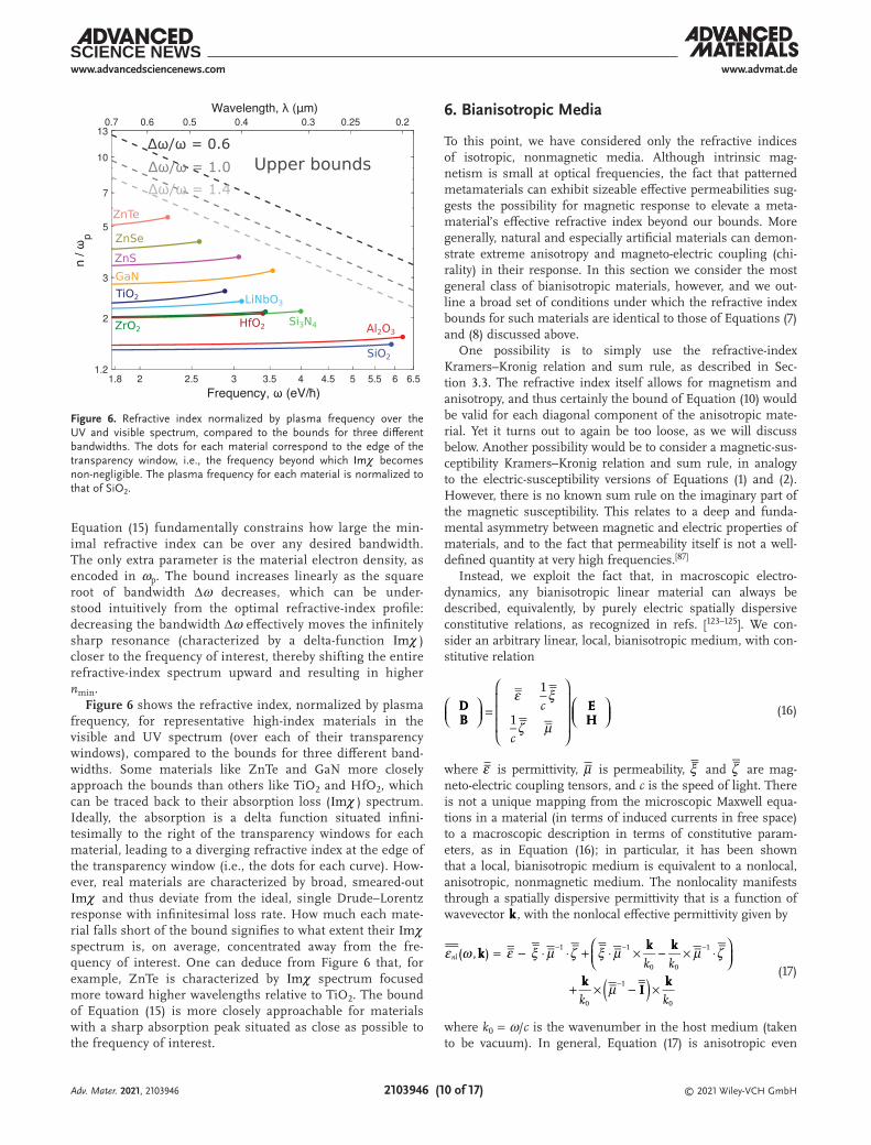
Equation  (15) fundamentally constrains how large the min-imal refractive index can be over any desired bandwidth. The only extra parameter is the material electron density, as encoded in ωp. The bound increases linearly as the square root of bandwidth Δω decreases, which can be under-stood intuitively from the optimal refractive-index profile: decreasing the bandwidth Δω effectively moves the infinitely sharp resonance (characterized by a delta-function χIm ) closer to the frequency of interest, thereby shifting the entire refractive-index spectrum upward and resulting in higher nmin.Figure 6 shows the refractive index, normalized by plasma

frequency, for representative high-index materials in the visible and UV spectrum (over each of their transparency windows), compared to the bounds for three different band-widths. Some materials like ZnTe and GaN more closely approach the bounds than others like TiO2 and HfO2, which can be traced back to their absorption loss ( χIm ) spectrum. Ideally, the absorption is a delta function situated infini-tesimally to the right of the transparency windows for each material, leading to a diverging refractive index at the edge of the transparency window (i.e., the dots for each curve). How-ever, real materials are characterized by broad, smeared-out

χIm and thus deviate from the ideal, single Drude–Lorentz response with infinitesimal loss rate. How much each mate-rial falls short of the bound signifies to what extent their χIm spectrum is, on average, concentrated away from the fre-quency of interest. One can deduce from Figure  6 that, for example, ZnTe is characterized by χIm spectrum focused more toward higher wavelengths relative to TiO2. The bound of Equation  (15) is more closely approachable for materials with a sharp absorption peak situated as close as possible to the frequency of interest.

6. Bianisotropic Media

To this point, we have considered only the refractive indices of isotropic, nonmagnetic media. Although intrinsic mag-netism is small at optical frequencies, the fact that patterned metamaterials can exhibit sizeable effective permeabilities sug-gests the possibility for magnetic response to elevate a meta-material’s effective refractive index beyond our bounds. More generally, natural and especially artificial materials can demon-strate extreme anisotropy and magneto-electric coupling (chi-rality) in their response. In this section we consider the most general class of bianisotropic materials, however, and we out-line a broad set of conditions under which the refractive index bounds for such materials are identical to those of Equations (7) and (8) discussed above.

One possibility is to simply use the refractive-index Kramers–Kronig relation and sum rule, as described in Sec-tion  3.3. The refractive index itself allows for magnetism and anisotropy, and thus certainly the bound of Equation (10) would be valid for each diagonal component of the anisotropic mate-rial. Yet it turns out to again be too loose, as we will discuss below. Another possibility would be to consider a magnetic-sus-ceptibility Kramers–Kronig relation and sum rule, in analogy to the electric-susceptibility versions of Equations (1) and (2). However, there is no known sum rule on the imaginary part of the magnetic susceptibility. This relates to a deep and funda-mental asymmetry between magnetic and electric properties of materials, and to the fact that permeability itself is not a well-defined quantity at very high frequencies.[87]

Instead, we exploit the fact that, in macroscopic electro-dynamics, any bianisotropic linear material can always be described, equivalently, by purely electric spatially dispersive constitutive relations, as recognized in refs.  [123–125]. We con-sider an arbitrary linear, local, bianisotropic medium, with con-stitutive relation

c

c

DDBB

EEHH

1

1

ε ξ

ζ µ

=

(16)

where ε is permittivity, µ is permeability, ξ and ζ are mag-neto-electric coupling tensors, and c is the speed of light. There is not a unique mapping from the microscopic Maxwell equa-tions in a material (in terms of induced currents in free space) to a macroscopic description in terms of constitutive param-eters, as in Equation  (16); in particular, it has been shown that a local, bianisotropic medium is equivalent to a nonlocal, anisotropic, nonmagnetic medium. The nonlocality manifests through a spatially dispersive permittivity that is a function of wavevector kk, with the nonlocal effective permittivity given by

k k

k k

nl kkkk kk

kkII

kk

( , )1 1

0 0

1

0

1

0

ε ω ε ξ µ ζ ξ µ µ ζ

µ( )= − ⋅ ⋅ + ⋅ × − × ⋅

+ × − ×

− − −

− (17)

where k0 = ω/c is the wavenumber in the host medium (taken to be vacuum). In general, Equation  (17) is anisotropic even

Adv. Mater. 2021, 2103946

Figure 6. Refractive index normalized by plasma frequency over the UV and visible spectrum, compared to the bounds for three different bandwidths. The dots for each material correspond to the edge of the transparency window, i.e., the frequency beyond which Imχ becomes non-negligible. The plasma frequency for each material is normalized to that of SiO2.

© 2021 Wiley-VCH GmbH2103946 (11 of 17)

www.advmat.dewww.advancedsciencenews.com

for isotropic permittivity and/or permeability, due to the wavevector dependence. In this case, we can utilize the fact that Kramers–Kronig relations and the f-sum rule are valid for each diagonal component and each individual wavevector of a spatially dispersive, anisotropic medium[125,126] (cf. Supporting Information). We can then represent the nonlocal suscepti-bility, Inl nlkk kk( , ) ( , )χ ω ε ω≡ − , where I is the identity tensor, as a sum of lossless Drude–Lorentz oscillators, exactly analogous to Equation (4). This is because we can always choose a polari-zation basis for which ( , )nl kkχ ω is diagonal, since it is Hermi-tian in the absence of dissipation. (Note that ( , )nl kkχ ω need not be diagonal for all frequencies ω and/or wavevectors kk under the same basis. However, we only require that ( , )nl kkχ ω is diag-onalizable at a given frequency and wavevector.)

The refractive index of an anisotropic medium is itself aniso-tropic, and depends also on the polarization of the electromag-netic field. Consider a propagating plane wave with wavevector

nckk s�ω= . The square of the bianisotropic refractive index,

nbianiso, experienced by that plane wave is one of two non-trivial solutions of the eigenproblem (cf. ref. [117], also see Supporting Information),

n Bnl bianisokk ee ee00 00( , ) 2ε ω = (18)

where B TII ss��= − and 0ee is the corresponding eigenvector that physically represents an eigen-polarization. For any mate-rial described by a positive- or negative-semidefinite ( , )nl kkε ω , the square of the refractive index in Equation  (18) is bounded by the largest eigenvalue of ( , )nl kkε ω (we defer the discussion of indefinite ( , )nl kkε ω to the end of this section). Choosing a polarization basis for which ( , )nl kkε ω is diagonal, the largest eigenvalue of ( , )nl kkε ω is its largest diagonal component. The magnitude of the diagonal components is bounded by their KK relations and sum rules, which individually degenerate to the isotropic bounds nmax,iso. (This sequence of steps is math-ematically proven in the Supporting Information.) Hence, the bianisotropic refractive index is bounded above by the isotropic-material bound:

n n≤bianiso max,iso (19)

Equation  (19) says that, no matter how one designs bianiso-tropic media, its maximum attainable refractive index, for any propagation direction and polarization, can never surpass that of isotropic, electric media, as long as ( , )nl kkε ω is positive- or negative-semidefinite. We can intuitively explain why mag-netism, chirality, and other bianistropic response cannot help increase the refractive index. Instead of viewing them as dis-tinct phenomena, it is helpful to view them as resulting from the same underlying matter, which can be distributed in dif-ferent ways to create different induced currents under the action of an applied electromagnetic field. For example, one can tailor the spatial dispersion of permittivity to obtain strong magnetic dipole moments, resulting in effective permeability, or alternatively, create strong chiral response, while the number of available electrons is always the same. Independent of the resulting bianisotropic response, they can all be described by the effective, nonlocal permittivity of Equation  (17) (with var-ying degrees of spatial dispersion), which is still subject to our

upper bound based on the total available electron density. Car-rying over our bound techniques employed in Section  3, the maximal refractive index for such ( , )nl kkε ω is therefore identical to Equation (7) with dispersion corresponding to the maximum principal component of ( , )nl kkε ω . We show in the Supporting Information that most bianisotropic media are captured by positive-definite ( , )nl kkε ω and also identify particular conditions (for example, magnetic materials with permeability greater than unity) under which ( , )nl kkε ω must be positive definite. Thus, our refractive-index bound is applicable to generic bianisotropic media that describe a wide range of metamaterials. This is a powerful result suggesting that, no matter how one designs metamaterials to include magnetic, chiral, or other bianiso-tropic response, the tradeoff between refractive index and dis-persion is inevitable.

The class of materials that have indefinite material ten-sors is exactly the class of hyperbolic (meta)materials.[127,128] In such materials, the bound of Equation (19) does not apply, and in fact there is no bound that can be derived. Mathematically, this makes sense: the indefinite nature of such materials leads to hyperbolic dispersion curves that can have arbitrarily large wavenumbers at finite frequencies, and consequently refrac-tive indices approaching infinity. Yet, physically, such waves are difficult to access as they are well outside the free-space light cone. Considering more realistic material models, based on microscopic and quantum-plasmonic considerations, this behavior is regularized by the introduction of: i) additional non-local effects, for example, hydrodynamic nonlocalities, which result in a large-wavevector cutoff in the material response[129] and ii) dissipation (e.g., Landau damping for large wavevec-tors). An interesting pathway forward would be to use com-putational optimization, for example “inverse design”,[91,130–133] to identify in-coupling and out-coupling structures that enable access to the high-index modes without reducing the index of the modes themselves.

Another case in which our bound does not hold is for gyrotropic plasmonic materials, the simplest example being a magnetized Drude plasma. Any conducting material has a pole at zero frequency that contributes an additional term in the KK relation for χIm , but in gyrotropic plasmonic mate-rials the zero-frequency pole can modify the KK relation for Re χ , altering Equation  (1) and the subsequent analysis.[134] Due to this additional term in the KK relation for Re χ , one can attain very large values of permittivity, and hence refrac-tive index, below the cyclotron resonance frequency with low loss and zero dispersion far away from resonance. Yet, such response only occurs below the cyclotron resonance frequency, which is typically much smaller than optical frequencies of interest for technologically available magnetic fields.

7. Designing High-Index Composites

In the previous sections we showed that for low to moderate dispersion values, natural materials already nearly saturate the fundamental bounds to refractive index. The high-dispersion, high-index part of the fundamental-limit curve has no com-parison points, however, as there are no materials that exhibit high dispersion in transparency windows at optical frequencies,

Adv. Mater. 2021, 2103946

© 2021 Wiley-VCH GmbH2103946 (12 of 17)

www.advmat.dewww.advancedsciencenews.com

and hence no materials exhibit the high refractive indices our bounds suggest should be possible. In fact, renormalization-group principles[60] have been used to identify the maximum refractive index in ensembles of atoms, yielding a value 1.7 that is close to those of real materials. Hence, an important open question is whether it is possible to engineer high refractive index, even allowing for high levels of dispersion?

Here, we show that composite materials can indeed exhibit significantly elevated refractive indices over their natural-material counterparts. Key to the designs is the use of metals and negative-permittivity materials, whose large susceptibili-ties unlock large positive refractive indices when patterned correctly. We find that with typical metals such as silver and aluminum, it should be possible to reach refractive indices larger than 10, with small losses, at the telecommunications wavelength 1.55 μm. The lossiness of the metals is the only factor preventing them from reaching even larger values; if it becomes possible to synthesize the “elusive lossless metal”,[15] with vanishingly small loss, then properly designed composites can exhibit refractive indices of 100 and beyond.

The theory of composite materials and the effective mate-rial properties that can be achieved has been developed over many decades.[138,139] Composite materials, or metamaterials, comprise multiple materials mixed at highly subwavelength length scales that show effective properties different from those of their underlying constituents. They offer a promising potential route, then, to achieving higher refractive indices through mixing than are possible in natural materials them-selves. Bounds, or fundamental limits, to the possible refrac-tive index of an isotropic composite have been known since the pioneering work of Bergman and Milton[135,136,140–142] (and even earlier for lossless materials[143]), and were recently updated and tightened.[137] Bounds are identified as a function of the fill frac-tion of one of the two (or more) materials. For composite of two materials, the bounds comprise two intersecting arcs in the complex permittivity plane. The analytical expressions for the

bounds are given in Equations (7) and (79) of ref. [137], which we do not repeat here due to their modest complexity.

In Figure 7, we demonstrate what is possible according to the updated Bergman–Milton bounds. At 1550 nm wavelength, we consider two classes of composite, one comprising a higher index dielectric material, germanium, with a low-index mate-rial taken to be air, and the second comprising a metallic mate-rial, aluminum, with the same air partner. The Ge-based com-posite exhibits only small variations in its possible refractive index, the red line, occupying the range between 1 (air) and 4.2 (Ge). By contrast, composites with aluminum can exhibit far greater variability, and potentially much larger real parts of their refractive index. The increasingly large regions occupied by the blue arcs represent the bound regions with increasing fill fractions of the aluminum. Of course, one cannot simply choose the highest real refractive index: most of those points are accompanied by tremendously large loss as well. Part (b) of Figure 7 zooms in on the lower left-hand side of the complex-n plane, where the imaginary parts are sufficiently small that the materials can be considered as nearly lossless. In that region, one can see that there are still sizable possible refractive indices. The largest loss rate can be defined as a ratio of the imaginary part of n to its real part. The real part determines the length over which a 2π phase accumulation can be achieved, while the imaginary part determines the absorption length, and the key criteria would typically be a large ratio of the two lengths. The black line in Figure 7b represents a loss-rate ratio of n nIm /Re 0.05= . One can see that refractive indices beyond 11 are achievable with an Al-based composite. Our predictive theory is corroborated by the results of ref. [92]. At the same 1550 nm wavelength, aluminum-based “space-filling” designs, albeit anisotropic, are predicted to exhibit refractive index com-ponents of ≈8 for the same loss-rate ratio (0.05), and up to 15 for n nIm /Re 0.2= . Our calculations suggest that an isotropic refractive index of almost 23 should be possible if one allows a loss rate of 0.2.

Adv. Mater. 2021, 2103946

Figure 7. The Bergman–Milton bounds,[135,136] recently strengthened,[137] identify the feasible effective material properties of isotropic composite mate-rials (metamaterials). a) Feasible regions for composites of germanium (red) versus aluminum (blue) at 1550 nm wavelength; in the latter case, each enclosed region represents a different fill fraction of aluminum relative to air. The large, negative susceptibility of aluminum enables strikingly large regions of high index, albeit also with nonzero losses. b) The low-loss portion of the feasible regions.

© 2021 Wiley-VCH GmbH2103946 (13 of 17)

www.advmat.dewww.advancedsciencenews.com

It is important to emphasize that the refractive indices shown in Figure  7b are indeed achievable. All of the low-loss bounds shown there, and below, arise from the circular arc that is known to be achievable by assemblages of doubly coated spheres.[137] The inset of Figure 8a schematically shows such an assemblage, comprising densely packed doubly coated spheres that fill all space (cf. Section 7.2 of ref. [138]). Figure 8a uses cir-cular markers to indicate the largest refractive indices that are possible, as a function of their dispersion values, for doubly-coated-sphere assemblages of aluminum and gold. (Silver is very similar to gold in its possible refractive-index values, due to their similar electron densities.) Accompanying the markers are solid lines that indicate the electron-density-based refrac-tive-index bounds of Equation  (7). One can see that the com-posites track quite closely with the bounds. Also included are markers for some of the highest-index natural materials, GaN, ZnTe, and GaAs, clearly showing the dramatic extent to which metal-based composites can improve on their natural dielectric counterparts. The figure does not go past dispersion values of 8 eV−1, however, as the losses of the composites grow too large in the designs for higher dispersion values. In Figure  8b, we map out the largest refractive indices as a function of wave-length that are possible with low-loss composites, with loss rates, as defined above, no larger than 0.05. With such compos-ites, refractive indices larger than 5, 18, and 40 are possible in the visible, near-infrared, and mid-infrared frequency ranges, respectively. Each would represent a record high in its respec-tive frequency range.

The large indices of the Al- and Au-based composites can be increased even further with lower-loss materials. To test the limits of what is possible, in Figure 9 we consider a com-posite with a lossless Drude metal with plasma frequency of 10 eV (corresponding to an electron density of 0.7 × 1023 cm−3). The updated Bergman–Milton bound, achieved by the doubly-coated-sphere assemblages, can now exhibit phenomenally

large refractive indices, even surpassing 100 in the infrared. As required by our bounds, such refractive indices are accompa-nied by phenomenally large dispersion values, and the inset shows the slow cube-root increase of refractive index with dispersion for these composites. Our bound of Equation  (7), applied to the Drude material, now lies along the curve for the composites, showing that the composites can saturate our bounds (and, consequently, that our bounds are tight and cannot be further improved). There is significant interest in engineering lossless metals;[15,16] if it can be done, we have

Adv. Mater. 2021, 2103946

Figure 8. Composites can achieve high refractive indices, at high levels of dispersion, as predicted by our bounds. a) At 1550 nm wavelength, typical high-index dielectrics such as GaAs and Ge have refractive indices approaching 4. By contrast, assemblages of doubly coated spheres (inset) of gold and aluminum can be designed to achieve low-loss, effective refractive indices above 8 and approaching 12, respectively. Moreover, these composites quite closely approach our bounds (solid lines), suggesting that they are tight or nearly so. b) Maximum low-loss refractive index of gold and aluminum composites as a function of wavelength. Much higher refractive indices are possible at longer wavelengths, as predicted by our bounds.

Figure 9. Lower-loss metals would enable even more dramatic enhance-ments of refractive index. Composites with a nearly lossless metal can be designed to achieve refractive indices larger than 100 at 1550 nm wave-length. These composites (circle markers) exactly achieve our bounds (solid line), and require enormous dispersion values to do so, thanks to the cube-root scaling indicated in the inset.

© 2021 Wiley-VCH GmbH2103946 (14 of 17)

www.advmat.dewww.advancedsciencenews.com

shown that refractive indices above 100 would be achievable at optical frequencies.

8. Conclusion

We have established the maximal refractive index valid for arbi-trary passive, linear media, given constraints on dispersion or bandwidth. Starting from Kramers–Kronig relations and the f-sum rule that all causal media have to obey, we have obtained a general representation of susceptibility. We have employed linear-programming techniques to demonstrate that the optimal solution is a single Drude–Lorentz oscillator with infinitesimal loss rate, which gives simple, analytic bounds on refractive index. Based on a similar approach, we have obtained bounds on high-index optical glasses and refractive index averaged over arbitrary bandwidth. We have also generalized our bounds to any biani-sotropic media described by a positive- or negative-semidefinite effective permittivity ( , )nl kkε ω , rendering our bounds more gen-eral than initially expected (i.e., the maximal refractive indices obtained in Sections  3 and 5 also describe materials incorpo-rating magnetic, chiral, and other bianisotropic response). We have also designed low-loss metal-based composites with refrac-tive indices exceeding those of best performing natural materials by a factor of two or more in the high-dispersion regime.

The approach developed herein can be extended to address a variety of related questions. For example, one can allow for gain media, which can still be described by a sum of Drude–Lorentz oscillators with infinitesimal loss rates (see Equation (4)). How-ever, the oscillator strengths in this scenario need not be posi-tive, leading to different optimal linear-programming solutions depending on the exact objective and constraints. In the case of gain media, stability considerations become crucial, as a high bulk refractive index, or any other bulk property, may be irrel-evant, if the resulting structure exhibits an unstable response with unbounded temporal oscillations.[144] Besides, while we have considered optical frequencies in this paper, the bounds established here can be used to compare state-of-the-art dielec-trics at microwave and other frequencies of interest. One may also be interested in metrics other than refractive index. A key metric in the context of waveguides and optical fibers is group velocity dispersion,[145] which can be seamlessly incorporated into our framework.

Another metric closely related to refractive index is the group index, which measures the reduction in group velocity of elec-tromagnetic waves in a medium. Unlike refractive index, the group index can reach values up to 60 even in the near-IR, and much higher elsewhere.[31] This is because group index ng, by definition, increases with dispersion:

nn

nn

g

d( )

ddd

ωω

ωω

= = + (20)

Very large values of group index are reached at large dispersion values dn/dω, for which the second term typically dominates the first, as it scales linearly with dispersion (whereas Equa-tion (8) restricts maximum n to scale with only the cube-root of dispersion). For example, electromagnetically induced transpar-ency can give rise to very sharp resonances in atomic vapors

and solids at cryogenic temperatures, leading to dispersion-dominated group indices even approaching 1010 (ref.  [31]). We show in the Supporting Information that bounds on group index averaged over arbitrary nonzero bandwidth can be obtained based on our refractive-index bound.

One can also explore negative (anomalous) dispersion, which typically occurs around resonances where losses are sizeable. To do so, one might construct other representations (such as B-splines[146]) that are more suited to describe regions of near-zero or negative dispersion.

An intriguing alternative extension is to nonlinear material properties. There are known Kramers–Kronig relations for non-linear susceptibilities,[147] yet their sum rules[80] are more com-plex than those of linear susceptibilities. If the sum rules can be simplified, or even just bounded, then it should be possible to identify bounds on nonlinear susceptibilities.

Another avenue that can potentially prove fruitful is to better understand the key characteristics of materials that determine refractive index. While the maximum allowable dispersion sets a limit on refractive index, are there more fundamental, physical quantities at play behind the scene? In the Supporting Information, we identify a characteristic trait of high-index materials: a combination of low molar mass and high elec-tronegativity, to achieve large valence electron densities. Such a “rule of thumb” is not a rigorous guideline (and may be espe-cially suspect for certain liquids and glasses), but can serve as a starting point for more rigorous ab initio approaches to identi-fying novel high-index materials.

Finally, direct experimental demonstrations of the high-index materials proposed in Section 7 would represent record refrac-tive indices. Techniques such as “inverse design”[91,130–133] may enable identification of structures with similarly high refrac-tive indices in architectures more amenable to fabrication than assemblages of doubly coated spheres. Identifying such com-posite materials would open new possibilities in areas from metasurface optics to high-quality-factor resonators. Each of these fields could benefit even more dramatically, potentially, with the discovery or synthesis of a near-zero-loss metal, which, as we have shown, could offer refractive indices approaching 100 at optical frequencies.

Supporting InformationSupporting Information is available from the Wiley Online Library or from the author.

AcknowledgementsThe authors thank Christian Kern for providing the illustration of an assemblage of doubly coated spheres. They also thank Jacob Khurgin, Michael Fiddy, and Richard Haglund for helpful conversations. H.S. and O.D.M. were supported by the Air Force Research Laboratory (AFRL and DARPA) under Contract No. FA8650-20-C-7019. F.M. was supported by the Air Force Office of Scientific Research under Grant FA9550-19-1-0043.

Conflict of InterestThe authors declare no conflict of interest.

Adv. Mater. 2021, 2103946

© 2021 Wiley-VCH GmbH2103946 (15 of 17)

www.advmat.dewww.advancedsciencenews.com

Data Availability StatementResearch data are not shared.

Keywordsclassical optics, light–matter interactions, metamaterials, optical materials, refraction

Received: May 25, 2021Revised: July 26, 2021

Published online:

[1] D.  Lin, P.  Fan, E.  Hasman, M. L.  Brongersma, Science 2014, 345, 298.

[2] A. Arbabi, Y. Horie, M. Bagheri, A. Faraon, Nat. Nanotechnol. 2015, 10, 937.

[3] M.  Khorasaninejad, W. T.  Chen, R. C.  Devlin, J.  Oh, A. Y.  Zhu, F. Capasso, Science 2016, 352, 1190.

[4] A. I.  Kuznetsov, A. E.  Miroshnichenko, M. L.  Brongersma, Y. S. Kivshar, B. Luk’yanchuk, Science 2016, 354, aag2472.

[5] J. Yang, J. A. Fan, Opt. Express 2017, 25, 23899.[6] E. Bayati, A. Zhan, S. Colburn, M. V. Zhelyeznyakov, A. Majumdar,

Appl. Opt. 2019, 58, 1460.[7] F. Presutti, F. Monticone, Optica 2020, 7, 624.[8] S. Noda, A. Chutinan, M. Imada, Nature 2000, 407, 608.[9] P. Michler, Science 2000, 290, 2282.

[10] M. Lončar, A. Scherer, Y. Qiu, Appl. Phys. Lett. 2003, 82, 4648.[11] J. P.  Reithmaier, G.  Se¸k, A.  Löffler, C.  Hofmann, S.  Kuhn,

S.  Reitzenstein, L. V.  Keldysh, V. D.  Kulakovskii, T. L.  Reinecke, A. Forchel, Nature 2004, 432, 197.

[12] T.  Tanabe, M.  Notomi, S.  Mitsugi, A.  Shinya, E.  Kuramochi, Appl. Phys. Lett. 2005, 87, 151112.

[13] K.  Hennessy, A.  Badolato, M.  Winger, D.  Gerace, M.  Atatüre, S. Gulde, S. Fält, E. L. Hu, A. Imamoğlu, Nature 2007, 445, 896.

[14] K. Srinivasan, O. Painter, Nature 2007, 450, 862.[15] J. B. Khurgin, G. Sun, Appl. Phys. Lett. 2010, 96, 181102.[16] A. Boltasseva, H. A. Atwater, Science 2011, 331, 290.[17] A. Li, S. Singh, D. Sievenpiper, Nanophotonics 2018, 7, 989.[18] A. Yariv, Quantum Electronics, 3rd edition, John Wiley & Sons, New

York 1989.[19] E. Yablonovitch, J. Opt. Soc. Am. 1982, 72, 899.[20] M. Kerker, D.-S. Wang, C. L. Giles, J. Opt. Soc. Am. 1983, 73, 765.[21] J. A. Schuller, R. Zia, T. Taubner, M. L. Brongersma, Phys. Rev. Lett.

2007, 99, 107401.[22] J. C.  Ginn, I.  Brener, D. W.  Peters, J. R.  Wendt, J. O.  Stevens,

P. F.  Hines, L. I.  Basilio, L. K.  Warne, J. F.  Ihlefeld, P. G.  Clem, M. B. Sinclair, Phys. Rev. Lett. 2012, 108, 097402.

[23] J.  Geffrin, B.  García-Cámara, R.  Gómez-Medina, P.  Albella, L.  Froufe-Pérez, C.  Eyraud, A.  Litman, R.  Vaillon, F.  González, M.  Nieto-Vesperinas, J.  Sáenz, F.  Moreno, Nat. Commun. 2012, 3, 1171.

[24] Y. H.  Fu, A. I.  Kuznetsov, A. E.  Miroshnichenko, Y. F.  Yu, B. Luk’yanchuk, Nat. Commun. 2013, 4, 1527.

[25] S. Person, M. Jain, Z. Lapin, J. J. Sáenz, G. Wicks, L. Novotny, Nano Lett. 2013, 13, 1806.

[26] R. M.  Bakker, D.  Permyakov, Y. F.  Yu, D.  Markovich, R.  Paniagua-Domínguez, L.  Gonzaga, A.  Samusev, Y.  Kivshar, B.  Lukyanchuk, A. I. Kuznetsov, Nano Lett. 2015, 15, 2137.

[27] F.  Monticone, A.  Alù, World Scientific Handbook of Metamaterials and Plasmonics, World Scientific Series in Nanoscience and Nanotechnology, World Scientific, Singapore 2017, pp. 295–335,

[28] A.  Vaskin, J.  Bohn, K. E.  Chong, T.  Bucher, M.  Zilk, D.-Y.  Choi, D. N. Neshev, Y. S. Kivshar, T. Pertsch, I. Staude, ACS Photonics 2018, 5, 1359.

[29] A.  Komar, R.  Paniagua-Domínguez, A.  Miroshnichenko, Y. F.  Yu, Y. S. Kivshar, A. I. Kuznetsov, D. Neshev, ACS Photonics 2018, 5, 1742.

[30] H. M.  Doeleman, F.  Monticone, W.  Den Hollander, A.  Alù, A. F. Koenderink, Nat. Photonics 2018, 12, 397.

[31] T. Baba, Nat. Photonics 2008, 2, 465.[32] T. F. Krauss, Nat. Photonics 2008, 2, 448.[33] J. T.  Robinson, C.  Manolatou, L.  Chen, M.  Lipson, Phys. Rev. Lett.

2005, 95, 143901.[34] X. Liang, S. G. Johnson, Opt. Express 2013, 21, 30812.[35] S. Hu, S. M. Weiss, ACS Photonics 2016, 3, 1647.[36] H. Choi, M. Heuck, D. Englund, Phys. Rev. Lett. 2017, 118, 223605.[37] Q. Zhao, L. Zhang, O. D. Miller, arXiv:2008.13241, 2020.[38] S. Nie, S. R. Emory, Science 1997, 275, 1102.[39] K.  Kneipp, Y.  Wang, H.  Kneipp, L. T.  Perelman, I.  Itzkan,

R. R. Dasari, M. S. Feld, Phys. Rev. Lett. 1997, 78, 1667.[40] T. S. van Zanten, A. Cambi, M. Koopman, B. Joosten, C. G. Figdor,

M. F. Garcia-Parajo, Proc. Natl. Acad. Sci. USA 2009, 106, 18557.[41] L. Schermelleh, R. Heintzmann, H. Leonhardt, J. Cell Biol. 2010, 190,

165.[42] H. O.  Marcy, L. A.  DeLoach, J.-H.  Liao, M. G.  Kanatzidis,

S. P. Velsko, M. J. Rosker, L. F. Warren, C. A. Ebbers, P. H. Cunningham, C. A. Thomas, Opt. Lett. 1995, 20, 252.

[43] M. Jain, H. Xia, G. Y. Yin, A. J. Merriam, S. E. Harris, Phys. Rev. Lett. 1996, 77, 4326.

[44] A. J.  Merriam, S. J.  Sharpe, M.  Shverdin, D.  Manuszak, G. Y.  Yin, S. E. Harris, Phys. Rev. Lett. 2000, 84, 5308.

[45] V.  Petrov, M.  Ghotbi, O.  Kokabee, A.  Esteban-Martin, F.  Noack, A.  Gaydardzhiev, I.  Nikolov, P.  Tzankov, I.  Buchvarov, K.  Miyata, A. Majchrowski, I. Kityk, F. Rotermund, E. Michalski, M. Ebrahim-Zadeh, Laser Photonics Rev. 2010, 4, 53.

[46] H. Shim, L. Fan, S. G.  Johnson, O. D. Miller, Phys. Rev. X 2019, 9, 11043.

[47] Z. Kuang, O. D. Miller, Phys. Rev. Lett. 2020, 125, 263607.[48] H. H. Li, J. Phys. Chem. Ref. Data 1980, 9, 561.[49] J. R. DeVore, J. Opt. Soc. Am. 1951, 41, 416.[50] J. Y. Kim, H. Kim, B. H. Kim, T. Chang, J. Lim, H. M. Jin, J. H. Mun,

Y. J. Choi, K. Chung, J. Shin, S. Fan, S. O. Kim, Nat. Commun. 2016, 7, 12911.

[51] J. Shin, J.-T. Shen, S. Fan, Phys. Rev. Lett. 2009, 102, 093903.[52] M.  Choi, S. H.  Lee, Y.  Kim, S. B.  Kang, J.  Shin, M. H.  Kwak,

K.-Y. Kang, Y.-H. Lee, N. Park, B. Min, Nature 2011, 470, 369.[53] C. Kittel, P. McEuen, Introduction to Solid State Physics, Vol. 8, Wiley,

New York 1996.[54] P.  Lunkenheimer, S. Krohns, S. Riegg, S. G. Ebbinghaus, A. Reller,

A. Loidl, Eur. Phys. J.: Spec. Top. 2009, 180, 61.[55] W. Hu, Y. Liu, R. L. Withers, T. J. Frankcombe, L. Norén, A. Snashall,

M.  Kitchin, P.  Smith, B.  Gong, H.  Chen, J.  Schiemer, F.  Brink, J. Wong-Leung, Nat. Mater. 2013, 12, 821.

[56] F.  Di Mei, L.  Falsi, M.  Flammini, D.  Pierangeli, P.  Di Porto, A. J. Agranat, E. DelRe, Nat. Photonics 2018, 12, 734.

[57] T. S. Moss, Proc. Phys. Soc., London, Sect. B 1950, 63, 167.[58] N. Ravindra, P. Ganapathy, J. Choi, Infrared Phys. Technol. 2007, 50,

21.[59] J. D. Jackson, Classical Electrodynamics, 3rd Ed., John Wiley & Sons,

Hoboken, NJ 1999.[60] F.  Andreoli, M. J.  Gullans, A. A.  High, A.  Browaeys, D. E.  Chang,

Phys. Rev. X 2021, 11, 011026.[61] M. G. Kuzyk, Phys. Rev. Lett. 2000, 85, 1218.[62] M. G. Kuzyk, J. Chem. Phys. 2006, 125, 154108.[63] J. Skaar, K. Seip, J. Phys. D: Appl. Phys. 2006, 39, 1226.[64] M. Gustafsson, D. Sjöberg, New J. Phys. 2010, 12, 043046.[65] M. I. Stockman, Phys. Rev. Lett. 2007, 98, 177404.

Adv. Mater. 2021, 2103946

© 2021 Wiley-VCH GmbH2103946 (16 of 17)

www.advmat.dewww.advancedsciencenews.com

[66] G. W. Milton, A. Srivastava, arXiv:2010.05986, 2020.[67] O. D.  Miller, A. G.  Polimeridis, M. T. H.  Reid, C. W.  Hsu,

B. G. Delacy, J. D.  Joannopoulos, M. Soljačic�, S. G.  Johnson, Opt. Express 2016, 24, 3329.

[68] J.-P.  Hugonin, M.  Besbes, P.  Ben-Abdallah, Phys. Rev. B 2015, 91, 180202(R).

[69] O. D.  Miller, O.  Ilic, T.  Christensen, M. T. H.  Reid, H. A.  Atwater, J. D. Joannopoulos, M. Soljačic�, S. G. Johnson, Nano Lett. 2017, 17, 5408.

[70] H. Zhang, C. W. Hsu, O. D. Miller, Optica 2019, 6, 1321.[71] G. Angeris, J. Vuckovic, S. P. Boyd, ACS Photonics 2019, 6, 1232.[72] S.  Molesky, W.  Jin, P. S.  Venkataram, A. W.  Rodriguez, Phys. Rev.

Lett. 2019, 123, 257401.[73] M. Gustafsson, K. Schab, L.  Jelinek, M. Capek, New J. Phys. 2020,

22, 073013.[74] S. Molesky, P. Chao, W.  Jin, A. W. Rodriguez, Phys. Rev. Res. 2020,

2, 033172.[75] R. Trivedi, G. Angeris, L. Su, S. Boyd, S. Fan, J. Vuckovic, Phys. Rev.

Appl. 2020, 14, 014025.[76] S. Molesky, P. S. Venkataram, W.  Jin, A. W. Rodriguez, Phys. Rev. B

2020, 101, 35408.[77] Z. Kuang, L. Zhang, O. D. Miller, Optica 2020, 7, 1746.[78] R. J. Vanderbei, Linear Programming, Vol. 3, Springer, Berlin 2015.[79] H. M.  Nussenzveig, Causality and Dispersion Relations, Academic

Press, Cambridge, MA 1972.[80] V. Lucarini, J. J. Saarinen, K.-E. Peiponen, E. M. Vartiainen, Kramers-

Kronig Relations in Optical Materials Research, Vol. 110, Springer Science & Business Media, Berlin 2005.

[81] F. Reiche, W. Thomas, Z. Phys. 1925, 34, 510.[82] W. Kuhn, Z. Phys. 1925, 33, 408.[83] F. W. King, J. Math. Phys. 1976, 17, 1509.[84] J. P. Boyd, Chebyshev and Fourier Spectral Methods, 2nd ed., Dover,

New York 2001.[85] M.  Cardona, Y. Y.  Peter, Fundamentals of Semiconductors, Springer,

Berlin 2005.[86] E.  Kaxiras, J. D.  Joannopoulos, Quantum Theory of Materials,

Cambridge University Press, Cambridge 2019.[87] L. D. Landau, J. S. Bell, M. J. Kearsley, L. P. Pitaevskii, E. M. Lifshitz,

J. B.  Sykes, Electrodynamics of Continuous Media, Vol. 8, Elsevier, Amsterdam, Netherlands 2013.

[88] J. Nocedal, S. J. Wright, Numerical Optimization, 2nd ed., Springer, New York, NY 2006.

[89] P.  Genevet, F.  Capasso, F.  Aieta, M.  Khorasaninejad, R.  Devlin, Optica 2017, 4, 139.

[90] W. T. Chen, A. Y. Zhu, V. Sanjeev, M. Khorasaninejad, Z. Shi, E. Lee, F. Capasso, Nat. Nanotechnol. 2018, 13, 220.

[91] H. Chung, O. D. Miller, Opt. Express 2020, 28, 6945.[92] T. Chang, J. U. Kim, S. K. Kang, H. Kim, D. K. Kim, Y.-H. Lee, J. Shin,

Nat. Commun. 2016, 7, 12661.[93] H. H. Li, J. Phys. Chem. Ref. Data 1980, 9, 161.[94] I. H. Malitson, J. Opt. Soc. Am. 1965, 55, 1205.[95] C. Tan, J. Non-Cryst. Solids 1998, 223, 158.[96] M. J. Weber, Handbook of Laser Science and Technology, Vol. 4, CRC-

Press, Boca Raton, FL 1986.[97] K. Luke, Y. Okawachi, M. R. E. Lamont, A. L. Gaeta, M. Lipson, Opt.

Lett. 2015, 40, 4823.[98] F. Peter, Z. Phys. 1923, 15, 358.[99] D. L. Wood, K. Nassau, T. Y. Kometani, D. L. Nash, Appl. Opt. 1990,

29, 604.[100] D. L. Wood, K. Nassau, Appl. Opt. 1982, 21, 2978.[101] D. E.  Zelmon, D. L.  Small, D.  Jundt, J. Opt. Soc. Am. B 1997, 14,

3319.[102] M. Debenham, Appl. Opt. 1984, 23, 2238.[103] C. A. Klein, Appl. Opt. 1986, 25, 1873.[104] A. S. Barker, M. Ilegems, Phys. Rev. B 1973, 7, 743.

[105] T.  Amotchkina, M.  Trubetskov, D.  Hahner, V.  Pervak, Appl. Opt. 2020, 59, A40.

[106] H. H. Li, J. Phys. Chem. Ref. Data 1984, 13, 103.[107] G. D. Pettit, W. J. Turner, J. Appl. Phys. 1965, 36, 2081.[108] T.  Skauli, P. S.  Kuo, K. L.  Vodopyanov, T. J.  Pinguet, O.  Levi,

L. A.  Eyres, J. S.  Harris, M. M.  Fejer, B.  Gerard, L.  Becouarn, E. Lallier, J. Appl. Phys. 2003, 94, 6447.

[109] D.  Chandler-Horowitz, P. M.  Amirtharaj, J. Appl. Phys. 2005, 97, 123526.

[110] O. G. Lorimor, W. G. Spitzer, J. Appl. Phys. 1965, 36, 1841.[111] J. H. Burnett, S. G. Kaplan, E. Stover, A. Phenis, in Proc. SPIE, Vol.

9974, SPIE, Bellingham, WA 2016, p. 99740X.[112] J. N.  Zemel, J. D.  Jensen, R. B.  Schoolar, Phys. Rev. 1965, 140,

A330.[113] R. S. Caldwell, H. Y. Fan, Phys. Rev. 1959, 114, 664.[114] G. C. Bhar, Appl. Opt. 1976, 15, 305.[115] F. Weiting, Y. Yixun, Infrared Phys. 1990, 30, 371.[116] Z.-c. Yan, G. W. F. Drake, Phys. Rev. A 1995, 52, R4316.[117] M. Born, E. Wolf, Principles of Optics: Electromagnetic Theory of Prop-

agation, Interference and Diffraction of Light, Elsevier, Amsterdam, Netherlands 2013.

[118] A. G. Schott Optical glass data sheets, https://www.schott.com/d/advanced_optics/ac85c64c-60a0-4113-a9df-23ee1be20428/1.17/schott-optical-glass-collection-datasheets-english-may-2019.pdf.

[119] J. B.  Hearnshaw, The Analysis of Starlight: One Hundred and Fifty Years of Astronomical Spectroscopy, CUP Archive 1990.

[120] H. Hovestadt, Jena Glass: And Its Scientific and Industrial Applications, Macmillan, London, NY 1902.

[121] L. Bergmann, C. Schaefer, Optics of Waves and Particles, W. de Gruyter, Berlin 1999.

[122] P. Hartmann, R. Jedamzik, S. Reichel, B. Schreder, Appl. Opt. 2010, 49, D157.

[123] V. M. Agranovich, Y. R. Shen, R. H. Baughman, A. A. Zakhidov, Phys. Rev. B 2004, 69, 165112.

[124] M. G. Silveirinha, Phys. Rev. B 2007, 75, 115104.[125] V. M. Agranovich, V. Ginzburg, Crystal Optics with Spatial Dispersion,

and Excitons, Vol. 42, Springer Science & Business Media, Berlin 2013.

[126] M. Altarelli, D. L. Dexter, H. M. Nussenzveig, D. Y. Smith, Phys. Rev. B 1972, 6, 4502.

[127] A.  Poddubny, I.  Iorsh, P.  Belov, Y.  Kivshar, Nat. Photonics 2013, 7, 948.

[128] L. Ferrari, C. Wu, D. Lepage, X. Zhang, Z. Liu, Prog. Quantum Elec-tron. 2015, 40, 1.

[129] W.  Yan, M.  Wubs, N. A.  Mortensen, Phys. Rev. B: Condens. Matter Mater. Phys. 2012, 86, 205429.

[130] J. S. Jensen, O. Sigmund, Laser Photonics Rev. 2011, 5, 308.[131] O. D. Miller, Ph.D. Thesis, University of California, Berkeley 2012.[132] S. Molesky, Z. Lin, A. Y. Piggott, W. Jin, J. Vucković, A. W. Rodriguez,

Nat. Photonics 2018, 12, 659.[133] T. Phan, D. Sell, E. W. Wang, S. Doshay, K. Edee, J. Yang, J. A. Fan,

Light: Sci. Appl. 2019, 8, 48.[134] M. I. Abdelrahman, F. Monticone, Phys. Rev. B 2020, 102, 155420.[135] D. J. Bergman, Phys. Rev. Lett. 1980, 44, 1285.[136] G. W. Milton, Appl. Phys. Lett. 1980, 37, 300.[137] C.  Kern, O. D.  Miller, G. W.  Milton, Phys. Rev. Appl. 2020, 14,

054068.[138] G. W. Milton, The Theory of Composites, Cambridge University Press,

Cambridge 2002.[139] G. W. Milton, Extending the Theory of Composites to Other Areas of

Science, Milton-Patton Publishers, Salt Lake City, UT 2016.[140] G. W. Milton, J. Appl. Phys. 1981, 52, 5286.[141] G. W. Milton, J. Appl. Phys. 1981, 52, 5294.[142] D. J. Bergman, Phys. Rev. B 1981, 23, 3058.[143] Z. Hashin, S. Shtrikman, J. Appl. Phys. 1962, 33, 3125.

Adv. Mater. 2021, 2103946

© 2021 Wiley-VCH GmbH2103946 (17 of 17)

www.advmat.dewww.advancedsciencenews.com

[144] B. Nistad, J.  Skaar, Phys. Rev. E: Stat., Nonlinear, Soft Matter Phys. 2008, 78, 036603.

[145] K. Okamoto, Fundamentals of Optical Waveguides, Academic press, Cambridge, MA 2006.

[146] Y. Ivanenko, M. Gustafsson, B. L. G. Jonsson, A. Luger, B. Nilsson, S. Nordebo, J. Toft, SIAM J. Appl. Math. 2019, 79, 436.

[147] R. W.  Boyd, Nonlinear Optics, Academic Press, Cambridge, MA 2003.

Adv. Mater. 2021, 2103946