hub arc selection for less-than-truckload …
TRANSCRIPT

HUB ARC SELECTION FOR
LESS-THAN-TRUCKLOAD CONSOLIDATION
____________________________________
A Master’s Thesis presented to the Faculty of the Graduate School
University of Missouri
_______________________________
In Partial Fulfillment
Of the Requirements for the Degree
Master of Science
________________________________
by
SEAN CARR
Dr. Wooseung Jang, Thesis Supervisor
DECEMBER 2008

The undersigned, appointed by the Dean of the Graduate School, have
hereby examined the Thesis entitled
HUB ARC SELECTION FOR
LESS-THAN-TRUCKLOAD CONSOLIDATION
Presented by Sean Carr
A candidate for the degree of Master of Science in Industrial
Engineering
And hereby certify that, in their opinion, it is worthy of acceptance
____________________________________ Dr. Wooseung Jang
____________________________________
Dr. James Noble
____________________________________
Dr. Lori Franz
____________________________________
Dr. Cerry Klein

ii
ACKNOWLEDGEMENTS
I would like to take this opportunity to thank those who have helped me along the
way, so that they know that I truly appreciate all they have done. I am very grateful to all
those who have made me the person I am today.
First and foremost, I thank my parents, David and Marcia Carr, for giving me
nothing but unconditional love my whole life. They have been the best parents one could
ask for. I also give great thanks to my grandparents for setting the best example possible
for me through their life experiences and family values. Family has always been of the
greatest significance to me.
Thank you to all the friends I have had the pleasure of making through my
formative and not-so-formative years. Friendship has made the journey much more
interesting and my friends mean a great deal to me.
I would also like to thank those that have shaped me through my work and school
experiences. During two summers of my high school years I worked in Nashville and
forged an ever-lasting relationship with the Van Ryens. They are truly great people and I
am forever indebted for the experience of living and working with them.
I also thank my undergraduate and graduate professors in the IMSE Department. I
would like to specifically thank Dr. James Noble and Dr. Wooseung Jang for giving me
opportunities to be a part of great undergraduate and graduate research projects. I also
thank Dr. Jang for advising my Master's Thesis. I learned a lot from him.
With respect to this research, I must thank the host company for providing an
intriguing and challenging problem as well as providing the problem data and I also thank
my company contact, Vijay Ramanathan for his help with the research.

iii
TABLE OF CONTENTS
ACKNOWLEDGEMENTS............................................................................ ii
TABLE OF CONTENTS................................................................................ iii
LIST OF FIGURES......................................................................................... v
ABSTRACT..................................................................................................... vii
Chapter
1. INTRODUCTION.................................................................................
1.1 Road Transportation...............................................................................
1.2 Freight Pricing and Economics..............................................................
1.3 Introduction to Consolidation Strategies................................................
1.4 Hub-and-Spoke Networks......................................................................
1.5 Introduction to the Proposed Models.....................................................
1
1
4
7
8
10
2. LITERATURE REVIEW......................................................................
2.1 Consolidation Strategy...........................................................................
2.2 Probabilistic Consolidation Policy.........................................................
2.3 Hub-and-spoke and Hub Network Models.............................................
2.3.1 Hub Location and P-Hub Problems
2.3.2 Non-restrictive Policies
2.3.3 Hub Covering Problem
2.3.4 Service Network Design Problems
2.3.5 Other Network Design Problems
2.3.6 Hub Arc Location Problem
2.3.7 Application
12
13
18
24
3. HUB NETWORK MODEL..................................................................
3.1 Model Objective.....................................................................................
3.2 Pitfalls of Previous Mathematical Models.............................................
3.3 Mathematical Formulation.....................................................................
3.3.1 Definitions 3.3.2 Formulation 3.4 Model Complexity.................................................................................
3.5 Specialized Solution Methodology........................................................
54
55
57
61
67 69
iv
3.5.1 Stage One: The Feasibility Check
3.5.2 Stage Two: Solve Sub-Model for Remaining Two-Hub
Scenarios
3.5.3 Stage Three: Resolve Duplicate Assignments
3.5.4 Stage Four: Integrate Local Solutions
4. CASE STUDY......................................................................................
4.1 Company Background............................................................................
4.2 Operations and Policy.............................................................................
4.3 Data Provided.........................................................................................
4.4 Consolidation Constraints.......................................................................
4.5 Data Preprocessing..................................................................................
4.5.1 Defining the Unit for Shipment Flow
4.6 Less-than-truckload Network.................................................................
82
82
83
85
86
87
90
5. EXAMPLE RESULTS..........................................................................
5.1 Model Parameters..................................................................................
5.1.1 Set of Origin and Destination Nodes and Flow Paths
5.1.2 Potential Hub Locations
5.1.3 Hub-to-Node and Hub-Hub Distances
5.1.4 Redefining Original LTL Costs
5.1.5 Other Model Parameters
5.2 LINGO Model........................................................................................
5.3 Case Results...........................................................................................
94
94
99
100
6. CONCLUSIONS...................................................................................
6.1 Conclusions............................................................................................
6.2 Extensions..............................................................................................
109
109
112
BIBLIOGRAPHY........................................................................................... 115

v
LIST OF FIGURES
Figure Page
1.1 Freight Providers such as FedEx provide LTL services.
1.2 Diagram of a Generic LTL transportation Network
1.3 Extensions of the Classic Hub-and-spoke Consolidation Model
3.1 Effects of Cumulative Shipment Waiting Time on Consolidation Performance
3.2 Summary of Definitions
3.3 Conflicting Sub-solutions
3.4 Origin-to-destination Flow Paths within a Potential Conflicting Scenario
3.5 Conflict Resolution Chart for Four Shared Flow Paths
4.1 Density Conversion Factors for Shipment Classes
4.2 Key Origins and Destinations of the Example LTL Network
5.1 Origin and Destination Flow Paths with Aggregated Flow
5.2 Locations of Potential Hub Facilities
5.3 List of Hub and Non-hub Nodes within each Local Service Region
5.4 Web Query to Calculate Distance between Nodes
5.5 LINGO Code
5.6 Excel Feasibility Matrix
5.7 Resulting Scenarios after Stage 1: Feasibility Check
5.8 Example Spreadsheet for sub-problem between Zip Codes 32837 and 30012
5.9 Example LINGO Results
5.10 Conflicting Solutions
5.11 Scenario 1 Variable Assignments and Objective Function Values
5.12 Scenario 2 Variable Assignments and Objective Function Values
1
8
9
60
63
78
79
80
89
93
95
96
96
97
100
101
101
102
103
104
105
106

vi
5.13 Hub Locations in the Global Solution
5.14 Summary of Consolidation Scenarios
5.15 Summary of Savings
106
107
108

vii
ABSTRACT
For more than twenty years, shipment consolidation has been utilized as a method
to significantly decrease the costs of transporting goods, people, and information. Due to
ever-increasing fuel costs and customer expectations, consolidation strategies are
becoming even more important in the freight transportation industry.
Using the hub-and-spoke model has also been widely recognized as an effective
design for shipment consolidation. This shipment consolidation takes advantage of
transportation economies of scale by gathering the shipments from clustered origins
around a transshipment center, called a hub, transporting them in bulk to other hubs, and
distributing the shipments to clustered destinations. Shipment delivery times and
transportation costs decrease as more and more shipments share vehicle capacity and
allow for more periodic service and increased vehicle utilization.
Previous research and literature have addressed consolidation and hub-and-spoke
network problems for years. However, many of the models focus on systems with larger
shipment volumes that allow for very efficient network configurations and operation. The
proposed research focuses on networks that consist of sparse or indefinite levels of
shipment quantities and unclear opportunity to consolidate the various origins and
destination.
This research proposes mathematical models and solution methodologies that will
determine the most advantageous set of hub-to-hub routes for the consolidation and
transportation of less-than-truckload (LTL) shipments, shipments that originally were
transported individually by commercial trucking. A global network model to identify uni-
directional (one-way) routes between sets of two hubs is proposed as a binary integer
viii
program. However, due to complexity concerns, a specialized methodology has also been
designed to solve the original problem by solving a set of sub-problems that combine to
form a global solution. The specialized methods include feasibility check, sub-problem
optimization, and conflict resolution stages.
Data from a Fortune-500 manufacturing company, describing a large-scale
domestic LTL network, has been provided as a case example for the proposed methods.
Results are provided in which 8 scenarios are identified to save transportation cost when
compared to previous policy. The methods can also be extended and tailored in a variety
of ways.
1
CHAPTER 1
INTRODUCTION
1.1 Road Transportation
Road and truck-based transportation are among the most significant modes of
freight transportation and their impact on the economy of the United States is revealed
through vast amounts of freight bill and freight volume. Road transportation includes
both Less-than-truckload (LTL) transportation and Full Truckload (FTL or TL)
transportation. The objective of these transportation methods is to delivery shipments
from dispersed origins to many other dispersed destinations in an efficient manner. While
some private, production-based companies use their own vehicle fleet and workforce to
provide these freight transportation services, there exists a large collection of commercial
carriers and third-party companies that plan and execute such services at a competitive,
yet profitable rate.
Figure1.1 Freight Providers such as FedEx provide Less-than-truckload services.

2
The difference between shipping LTL and TL is substantial. Full Truckload
transportation is usually reserved for one large shipment bound for just one destination or
very few closely-located destinations. Because TL shipments are relatively large, there is
little to no opportunity for the consolidation of shipments from multiple origins due to
vehicle storage space and weight constraints.
Service providers of full truckload transportation can be small, single-location
operations that service a small region or they can be large companies with intricate
transportation networks. These service providers, or carriers, typically provide one-way
service from origin to destination. By making arrangements with customers in the
vicinity of various destinations, the truckload provider can control the movement of
trucks so as to reduce the amount of empty travel and backtracking, called back-haul,
while giving the vehicle drivers the opportunity to return home for rest and time off.
Larger truckload carriers can also create their own network of routes that service a very
large area and determine effective relay points to allow their drivers to return to their
respective homes.
Commonly, truckload carriers use the largest available vehicles to ship larger
orders at one time. The standard trailer has recently expanded from 48 to 53 ft long and
approximately 8 feet wide and 10 feet tall. Often, TL carriers can offer other specialized
service for specific product groups such as oversized loads, hazardous material, or
refrigeration for perishable items. For safety reasons, government regulations restrict full
truckload gross weight to 80,000 pounds, which includes the weight of the empty
trailer(s) and truck as well1. The weight of any empty truck and trailer can exceed 30,000
1 Regulations available at www.dot.gov > Federal Highway Administration Freight Management and
Operations>Vehicle Size and Weight> Regulation 23 CFR 658

3
pounds, leaving approximately 50,000 pounds for freight. Therefore, trucks may “weigh-
out,” or become full with respect to weight limits. Similarly, due to the variety of sizes
and shipment composition, full trailers may also “cube out” when the weight limit has not
been reached but the overall trailer volume has been fully utilized. Truckload rates are
typically quoted on a per-mile basis that is dependent upon delivery geography, accessory
services, and delivery deadline.
Less-than-truckload transportation is very different from TL from both an
operational and physical perspective. LTL carriers do business with all types of
organizations from small businesses to large manufacturing companies. The objective of
these carriers is to transport as many small shipments from a large number of origins as
possible. The LTL carriers may perform local pickup functions from shipment origins
and transport them to their own facilities, called hubs. In academia and industry alike,
hubs go by many names such as transshipment points, distribution centers, make-
bulk/break-bulk centers, etc. At these points, shipments from many origins consolidate
into larger vehicles, which are loaded with shipments that will be transported to closely
located destinations. These trucks will transport the full trucks to another hub location,
where the individual shipments will be dispersed to their respective destinations. Trucks
used for longer distances of LTL transportation are similar to those used for full
truckload, and have similar weight and volume constraints. The same government
regulations affect how much they can carry in weight.
In many ways, an LTL carrier employs TL strategies over long distance routes,
called long-haul, but has the resources to service well-dispersed locations through
extensive networks that may include more than several dozen hubs nationwide. In fact,

4
the LTL networks of companies like Yellow Freight or FedEx may consist of more than
one hundred transshipment terminals. Transshipment terminals are centralized facilities
that are used to very highly utilize vehicle space by combining shipments from different
regions that are bound for similar destination areas. The extensive networks employed by
LTL carriers to transport goods from very large numbers of origins to even more
destinations are often referred to as hub-and-spoke, or simply hub networks.
For shipments that travel relatively long distances, such as cross-country, the
process of pickup, long-haul, and delivery may take an individual shipment through a
series of several hub facilities, depending on the configuration and scope of that
particular carrier’s network.
A shipment or set of shipments from a common origin is usually classified Less-
than-Truckload when it weighs more than 100 pounds (less than 100 pounds would
typically be considered parcel) and less than 20,000 pounds. Shipment dimensions also
greatly affect the decision to ship something LTL. For example, single shipments longer
than 12 feet may be shipped TL. Naturally, shipments with very large weight or with very
low density are commonly shipped TL because LTL companies want to ship many
individual orders at once, making vehicle capacity very valuable.
1.2 Less-than-truckload Pricing and Economics
The process of pricing LTL shipments is relatively complex. Typically, rates are
based mostly on freight class. The National Motor Freight Association determines the
National Motor Freight Classification, which defines the class for nearly all possible

5
items that might be shipped using LTL. This class is based primarily on product density,
but also includes other factors like item value and fragility, or "loadability". Classes
range from 50 to 500, which represent the percentage factor applied to a base rate.
Typically, denser materials carry a rating lower than 100, thus reducing the base rate.
Rates are determined by geographic location of the origin and destination as well. The
resultant LTL rates are quoted on a per-100 pound (termed "cwt") basis. Therefore, a 200
pound shipment rated at 112 cwt would cost $224 to ship. LTL carriers may also give
significant discounts of greater than 50 % through contractual agreements with corporate
customers that ship very high quantities.
In return for convenience and assurance of safe transport, LTL carriers demand
high rates per shipment from customers, while still maintaining the cost feasibility of the
customer. These customers typically could not afford to send each shipment directly to its
destination, while maintaining strict shipping deadlines, without some method to
significantly reduce the many fixed, variable, capital and operating costs of long-haul
transportation. For the private company to justify using their own transportation
resources, they must cover several costs, such as the leasing or purchasing of vehicles,
the cost of additional storage space for the storage and handling of shipments, the costs of
maintaining a dedicated workforce responsible for freight shipment and handling, and the
fuel energy costs of operating freight vehicles. Therefore, one major method of reducing
these costs, which increase with the number of shipments made, has been to consolidate
many smaller shipments into a larger vehicle to be transported together, thus sharing the
total cost among each shipment.
6
Unfortunately, companies should also be warned of the disadvantages of private
shipment consolidation. Most methods of shipment consolidation increase inventory
holding time of shipments, which may affect customer relationships. In addition, the
common company may not have enough consolidated shipments to make up for the large
costs of operating its own transportation network. Therefore, smaller companies with
limited shipments may be at the mercy of the public LTL carrier.
However, larger companies that have the adequate resources and shipment
volume to consolidate have a strong case for private LTL transportation. Firstly, the
commercial LTL company's network often consists of both regional and local hubs that
are used for transshipment and distribution operations. Therefore, the process of an
individual shipment from the customer travelling through an extensive network with
multiple stops often results in longer travel times, compared to more dedicated routes.
Secondly, shipments that are loaded and unloaded several times during the course of
travel are subject to the inherent chance of shipment damage. Although commercial LTL
carriers uphold certain operational standards, accidents do happen. By efficiently
acquiring the physical resources and reallocating existing resources, private consolidation
by an organization through its own transportation network can be a profitable venture.
Because private LTL carriage introduces an opportunity for companies to
significantly decrease logistics cost, it will be the main focus of this research, specifically
the smaller company with limited shipment quantities.

7
1.3 Introduction to Consolidation Strategies
For both the commercial carrier and the company that decides to use private
transportation resources for less-than-truckload shipments, there are three major types of
freight consolidation strategies or techniques used to decrease costs. The first strategy is
multi-stop consolidation, where less-than-truckload shipments are picked up and dropped
off at respective locations by the same vehicle through multiple-stop routes. The second
strategy is often referred to as temporal consolidation, where shipment schedules within
one facility are adjusted so that many shipments are shipped using single large shipment.
The third strategy is considered facility consolidation, where small shipments among
several facilities travelling long distances are consolidated into large shipments travelling
large distances and small shipments over small distances [13].
For many manufacturing companies, temporal and facility consolidation tend to
apply best because a large majority of the freight movement takes place between dense
areas of production (manufacturing facilities or other shipment origins) and consumption
(retailers or other vendors). Therefore, hub networks can be set up so that shipments that
originate within a common area can combine together to make full truckloads that travel
to closely-located destinations. This will allow the shipper to utilize their vehicles better
and share the transportation cost among more shipments, effectively outweighing the cost
of sending each order individually.
8
1.4 Hub-and-spoke Networks
In recent years, hub-and-spoke networks have been implemented within the
telecommunication and airline industries and applied by both parcel and freight carriers.
These industries greatly rely on methods to reduce overall network costs, including
transportation and infrastructure cost. Fortunately, the opportunity may be present for the
private enterprise to implement the same models to effectively minimize transportation
costs. Hub models allow for the sharing of transportation costs by utilizing larger vehicles
along common, direct routes, thereby distributing the transportation cost among large
shipment quantities. These types of models can take great advantage of clustered origins
and destinations that are capable of encompassing large numbers of individual shipments.
In freight delivery applications, the hubs represent transshipment locations for
consolidating smaller LTL shipments from various origins and de-consolidating the
shipments before distributing them to their respective destinations. The hub facilities
typically have a defined "service radius", which would determine which individual origin
and destination facilities that can utilize the hub facility for consolidation. The spokes
then represent the routes used for pickup and delivery operations. Networked hub models
include several interconnected hub-and-spoke systems so that shipments from a wider
range of origins travelling to a wider range of destinations can take advantage of
consolidated transportation. Larger hub networks allow each individual shipment to take
a choice of routes that allow for more opportunities to find significant logistics cost-
saving configurations.

9
Figure 1.2 Diagram of a Generic LTL Transportation Network.
Other modifications to the basic hub-and-spoke configuration exist to share the
truckload transportation cost among a larger amount of shipments, which effectively
lowers the total cost of transportation (or results in higher cost savings when compared to
less-than-truckload transportation). The first extension to the classic hub-and-spoke
model is a hub-and-spoke configuration with added LTL transportation. This model is
utilized in instances when LTL cost is sufficiently lower for shorter distances, so that
shipments can be added to a consolidated route with little additional cost. Another model
is the classic hub-and-spoke model with intermediate hubs, where significant shipment
volumes are dropped off for distribution, other shipments may be picked up, and the main
route is continued to other hub locations. Other approaches include expanding the
service radius to consolidate more origins and destinations.

10
Figure 1.3 Extensions of the Classic Hub-and-spoke Consolidation Model
1.5 Introduction to the Proposed Models
In this research, the classic hub-and-spoke configuration without extension will be
the underlying model used with a mathematical programming framework to solve less-
than-truckload consolidation problems. The decision to implement a shipment
consolidation policy is not an easy one for the private company with limited shipments;
therefore, a method to help determine if consolidation is advantageous is much needed.
It has been argued that a private shipment consolidation and transportation
strategy can decrease logistics costs by taking advantage of transportation economies of
scale. The proposed model will be especially suited for the organization that currently
relies on transportation service providers to deliver relatively smaller amounts of
shipments to highly dispersed destinations. The model will also be better utilized by

11
companies with a well-documented history of less-than-truckload costs, origin and
destination locations, and demand.
The mathematical model in the form of an integer program will define an existing
distribution network consisting of shipment flow paths from several origins to several
destinations, with each flow path described by the total amount or size of shipments.
Each flow path will also be associated with the per-unit cost of direct transportation. A
set of potential hub locations will be defined to act as consolidation centers where
shipments from origins within a defined local service region will be gathered and shipped
together to other consolidation centers, where they are distributed to their respective
destinations. The fixed cost per trip of consolidated transportation between hubs will be
defined as well as the per-unit cost of local transportation from each hub to its serviceable
origin and destination points. Space constraints will be set to limit the total amount of
shipments that a consolidated truckload vehicle can transport at one time.
The goal of the mathematical model is to determine the set of one-way routes
between two hubs, called hub arcs, which can be used for less-than-truckload
transportation. Only routes that result in less transportation cost than previous less-than-
truckload costs are chosen. Along with routes, the most beneficial assignment policy for
the various origins and destinations will be determined. A specialized solution
methodology is developed to solve the model.

12
CHAPTER 2
LITERATURE REVIEW
Much research has been conducted to investigate and model consolidation
strategy and hub-and-spoke networks with applications in the fields of transportation
logistics and distribution. For more than 20 years, strategical issues have been studied,
including the effects of important network configuration parameters like dispatching
policy and number of consolidation facilities on customer service issues like
consolidation cycle time. Probabilistic models were employed to determine optimal
operational aspects of consolidation like shipment dispatching. Hub-and-spoke models
began as facility location problems and relied on mathematical programming to locate
one hub within a set of demand nodes to model the distribution of goods from warehouse
to retailer. Models varied in objectives, but typically minimized the total transportation
cost of satisfying all demand points. Soon thereafter, facility location problems were
extended to model the transportation of shipments from origin to destination. To
determine the current state of consolidation research, literature in each of these uniquely
significant areas was reviewed. The major issues that this literature review addresses are
consolidation strategy, probabilistic models, and mathematical models used to determine
optimal hub network design.
The models proposed in this research will be inspired by the uncapacitated hub
network design problem and hub arc location problem. While hub network design
problems such as the p-hub median and hub location problem minimize total

13
transportation costs by changing hub location and node assignments, the hub arc location
problem determines the best subset of hub-to-hub arcs that should be opened for
consolidated truckload service.
The literature that most inspired the proposed model are the Cluster Hub Location
problem (CHLP), first formulated by Wagner in 2001[32, 33], and the Hub Arc Location
problem (HAL), formulated by Campbell et al. in 2007[6, 7]. The contribution of the
CHLP to this research is a non-restrictive node assignment policy, where each origin-to-
destination path of shipment flow can choose to use direct service, comparable to LTL, or
use a hub-to-hub route representing consolidated truckload service. The main
contribution of the Hub Arc Location problem is a focus on choosing arcs that would
ensure enough volume to sustain relatively full and frequent service and justify the
assumption of economies of scale. The Hub Arc Location problem assumes, however,
that all shipment origins and destinations must utilize the resulting consolidation network.
2.1 Consolidation Strategy
Significant research in consolidation strategy began in the early 1980's, when
consolidation was first revered as an effective method to significantly decrease costs of
delivering people, goods, and information. This research concentrated on the many
variables that affect the performance of consolidation practices with respect to both cost
and service level considerations.
In 1980, Masters [25] authored “The effects of freight consolidation on customer
service.” Masters noted that other factors besides cost affect the effectiveness of

14
consolidation strategy. The average and variance of consolidation cycle times are of
particular importance. This research addressed the affects of consolidation on both cost
and delivery time.
In his research, the number of geographic regions, maximum holding time for
shipments, the design of the network, and the network objective were studied because the
choice between minimizing cost, distance, and delivery time all affect where
consolidation facilities are located and to what facility each customer is assigned.
Discrete event computer simulation was used in his research to test consolidation
strategies when varying customer order quantities and consolidation methods.
The example network consisted of 399 points representing customer demand with
shipment quantities proportional to population, 73 potential consolidation facilities, and
only one source of order production located near Columbus, Ohio. A heuristic algorithm
was used to create different scenarios, or configurations, that varied in number of
consolidation facilities, costs, and time parameters. Masters performed an ANOVA to test
the significant difference between configurations. The model used for the heuristics
assumed deterministic flow, fixed order size, and uniform arrival rates. A search
algorithm was used to locate the best consolidation points among the same region.
Results showed that all main factors were significant. The main conclusions were
that freight consolidation reduces transportation cost, increases mean delivery time but
does not increase the variance of delivery time. Among all factors, order characteristics
greatly affect performance of a shipment consolidation policy.
In 1981, Jackson [16] published “Evaluating order consolidation strategies using
simulation.” The paper studied the effects of the number of pool points (hubs), length of

15
maximum holding time, and the shipment release strategy (such strategies will be
discussed in more detail in the next section). This research includes the application of a
medium-sized company’s shipments with an average order size of 1,300 pounds. A
simulation model was used to run experiments to test the affects of four factors, number
of consolidation points, orders per day, order release strategy, and maximum holding
time. The three measures were average cost per consolidation cycle, average cycle length,
and the variance of cycle length.
It was determined that longer shipping intervals resulted in lower costs.
Consolidation cycle times also increased for low-volume systems. With respect to the
number of pool points, high volume and longer holding time justify more pool points.
With respect to shipment release strategies, a schedule-based was cheaper, but slower,
than using a combination of a scheduled- and weight-based strategy.
In 1984, Cooper [9] published “Cost and Delivery Time Implications of Freight
Consolidation and Warehousing Strategies.” In this research, performance measures were
studied for varying distribution strategies including traditional LTL from a warehouse,
consolidated shipments from plants and warehouses, and LTL from plants. The variables
that were studied were shipment holding time, quantity of annual orders, mean order
weight, product classification, geographic distribution of demand, and plant location. A
total of 96 combinations of factors were analyzed. A branch and bound procedure was
used to select the warehouse locations from a set of 40 metropolitan areas. Each of the 96
factor combinations were simulated using a batch-run of 250 days.
The main results of the research concluded that waiting four days as opposed to
just one was always the lowest cost system. Among all variables, mean order weight
16
accounted for the most variance in the system. Mean order weight, product class, and
annual orders also affected consolidation costs. In addition, the system with the lowest
mean delivery time was not always the system with the lowest delivery time variance.
Results also concluded that direct LTL shipping was more expensive than
consolidated shipping. However, for holding periods of just one day, the volume is not
sufficient enough to save transportation cost. Lower product classes also required fewer
consolidation points because of a decreased need for more consolidation points to reach
weight-based discount points.
In 1986, Jackson [17] continued research on consolidation with “A survey of
freight consolidation practices.” This research was a study of the state of consolidation
strategy by approximately 50 companies practicing freight consolidation. The author
attempted to study why and how these companies use consolidation. The author used
questionnaires to gather information from companies across more than 10 industries
about their consolidation practices and strategy. More than half of these companies were
in the manufacturing industry.
The first topic discussed deals with the reasons companies engage in freight
consolidation. The authors reported that 84 % of companies found consolidation very
important for cost reasons, and 77 % found consolidation beneficial for service. Among
the cost factors, companies reported transportation cost reduction was more motivation
than inventory carrying costs. Among the service level factors, the reduction of transit
time was of the highest importance. The main disadvantages reported were longer order
cycle and staffing.

17
The second topic was the operational aspects of consolidation. The average
maximum waiting or holding time for consolidated orders was around 2.7 days, with the
most reported being 3 days. Also, 74 % of companies attempted to consolidate rush
orders as well. Although no one dispatching rule for consolidation was reported, the most
common methods were “scheduled sailing,” which dispatches orders to a consolidation
facility on a specific day, and another method that uses the earlier occurrence of reaching
a scheduled shipment date or weight limit. The average number of hub facilities was 20,
with some companies reporting employing up to 130 hubs. Drop points were reported as
performed frequently by more than 60 % of carriers, with only 1 stop being the most
common.
The research also discussed the problems that arose for the companies
consolidating shipments. The most common reported problems were meeting scheduled
deliveries and customer service, availability of orders for consolidation, over, short, and
damaged deliveries, and educating salespeople and customers. The most common reasons
for failure of a consolidated shipment was from insufficient volume and customer service
and timing issues.
In 1992, Pooley and Stenger [29] published “Modeling and evaluating shipment
consolidation in a logistics system,” to discuss consolidation strategy when using a mix
of multi-stop TL service and supplemental LTL service. The authors cited that 97% of
firms that used some sort of consolidation used a multi-stop strategy.
The authors studied five factors that affect logistics system performance using a
consolidation strategy. Network Design factor explores the significance of shipments on
different lanes being independent. Mean order size, consolidation cycle time constraint,

18
LTL discounts, and geographic distribution of customer demand were also considered
important factors.
Experiments to test the five factors on two consolidation strategies, vehicle
routing and multi-stop, were conducting using data from two cases of shippers. One firm
has two manufacturing plants and 4 distribution centers. The second firm has one central
plant that distributes nationally. Results were found using three methods of computation:
a shipment consolidation heuristic algorithm, computer simulation, and a MIP
mathematical model. Experimental design was used to create a 2k full factorial design, for
which ANOVA was performed to determine significance of factors.
Results showed that the level of LTL discount, an increased cycle time, and
larger-sized orders lowered costs. The distribution of orders was shown to have little to
no effect. The most telling result of this study was that results did vary significantly
between firms. Therefore, it is also concluded that consolidation strategy might be
affected by the specific problem instance.
2.2 Probabilistic Consolidation Policy
With respect to operational aspects such as consolidated shipment dispatching,
other methods for determining effective consolidation policy have involved stochastic
methods such as stochastic clearing systems and arrival processes. The objective of these
models have been to determine the optimal consolidation strategy with respect to how
long a consolidation cycle continues to wait for incoming shipments. Such decisions can
be dependent on vehicle capacity restrictions as well as inventory holding costs.

19
Therefore, incoming shipments are typically described by stochastic arrival processes
according to a probability distribution and the arrival process of consolidating incoming
shipments to a hub has been of interest.
In 1994, Higginson and Bookbinder [14] published “Policy recommendations for
a shipment-consolidation program,” to discuss the decisions involved for a consolidation
program with respect to the method of consolidation under various assumptions. The
questions addressed were 1) Which orders should and should not be consolidated, 2)
What triggers the dispatch of a consolidated load, 3) Is consolidation performed at the
factory, vehicle, or warehouse, 4) Who performs the consolidation, the shipper, customer,
or carrier, 5) What techniques will be used, and 6) As each order arrives, do we ship now
alone, consolidate, or delay for future consolidation.
The factors that the authors considered most important to answer the
aforementioned questions are the number of current unshipped orders, company policy,
order due date, order destination, order type, weight, volume, and size, transportation
mode, vehicle capacity, transportation cost, and inventory holding cost.
The authors then describe the three major dispatching policies used for order
consolidation. A time policy dispatches consolidated orders at a specific date or time
regardless of the amount of consolidation. For example, the shipment may be released
when the oldest order reaches a certain age. A quantity policy holds orders until a total
weight is reached. Finally, a time-and-quantity policy holds a shipment until the earlier of
the two previous events occurs.
To begin their research, the authors used the Economic Shipment Weight (ESW)
model (similar to Economic Order Quantity in inventory theory) to determine the optimal

20
load size that would minimize the transportation and inventory holding costs per order
subject to varying target weights (or weight limits). These constraints represent vehicle
capacity or other organizational policy. Results were also determined for varying
maximum waiting time of an order, including .75 days, 1, 1.5, 2 days, as described in the
time policy. The authors used a simulation model to test the unit costs and delay for the
three possible policies. The authors use a Poisson arrival process, and Gamma-distributed
order weights. A Paired-T test was used for testing significance between policies.
Key results showed that low arrival and low due dates yield a different policy than
high arrivals and long holding times. In addition, no one policy yielded a lowest per unit
cost for all arrival rates. The time-and-weight policy yielded the smallest delay per order.
The quantity policy performed well for short holding time allowances. The time policy
resulted in very small loads for low arrival rates. The time policy also resulted in small
holding times and performed better in this category than the time-and-weight policy.
However, inventory costs overwhelm the time policy for cases of frequent arrivals and
increased holding time. The time-and-quantity policy performs well for short holding
time and but not as well as the quantity policy. For cases of low arrival rates and short
holding times, the time-and-quantity policy was more expensive than a time policy. The
time-and-quantity policy also resulted in a respectable unit-cost but performed the best
among policies with respect to order delay.
The authors also refer back to Jackson [17], which found that low volume systems
suffer from greater transportation costs and more order delays. The authors suggest that
the combination of high arrivals and long holding time results in lower costs if the
holding costs are ignored. Otherwise, holding costs will overwhelm transportation costs.
21
Overall, the time strategy is performs better with respect to the addition of transportation
and inventory holding cost, but is slower for high volume systems and comparable to
other policies for low order volumes.
In 1995, Higginson [14] published “Recurrent decision approaches to shipment-
release timing in freight consolidation.” A recurrent decision model re-evaluates the
release decision after every shipment arrives as opposed to the static release point
determined by deterministic economic quantities. Due to the stochastic nature of
customer orders, the non-recurrent approaches in other research often lead to less than
optimal release points, as Economic Shipment Weight/Quantities (ESW/ESQ) are
dependent upon only average weight, average arrival parameters, and average inventory
holding costs.
In this paper, recurrent models are built and analyzed from both private and
commercial carrier perspectives. A marginal analysis framework is used. As each
shipment arrives, it is determined if we should wait until the next order arrives or
dispatch immediately based upon stochastic shipment arrival and weight behavior.
The private carrier model assumes a fixed transportation cost and physical
capacity constraints. Simulation results were given using Gamma-distributed weights,
Poisson arrivals, and a vehicle capacity of 40,000 pounds. The proposed model yielded
smaller delay for all arrival rates, but also tended to be more expensive than the
deterministic ESW.
The common carrier model assumed fixed transportation cost, but allowed for
unlimited capacity. In addition, customer service constraints restricted the order holding

22
time. The common carrier model outperformed the ESW with respect to cost. However,
delay was increased.
In 2002, Bookbinder and Higginson [1] published “Probabilistic modeling of
freight consolidation by private carriage” describing a stochastic clearing system
approach to freight consolidation including consolidation quantity and related dispatch
timing.
In the first example, the authors show how to find the probability of meeting a
target weight by a specified time deadline, for which a closed form solution exists. The
information gained from this type of problem can be used in a number of cases. The first
case is when a target weight is less than vehicle capacity and the second case is when the
target weight equals capacity. In the latter case, the probability also gives the percentage
of vehicle capacity that will be utilized when the time deadline arrives. The deadline
resultantly represents the maximum allowable inventory holding time, assuming
homogenous orders.
Next, the authors apply the previous probability concepts towards optimizing the
holding quantity when considering inventory holding cost and bulk transportation cost.
When considering the quantity of accumulated arrivals and the clearing system, the time
between clearings represents a renewal process. In this process, the number of
accumulated arrivals after each clearing is identically distributed. The optimal holding
quantity minimizing total costs can be found based on the time it takes to reach certain
levels of consolidation. In the cost equation, there are parameters to describe the cost per
unit and a function describing the cost per unit time versus holding quantity. Solving for
the optimal quantity may be possible in closed form or by computing the integral of the

23
cost function. In addition, a method to find the optimal consolidated weight when the
inter-arrival distribution and weight distribution are converted to a joint “order-weight”
gamma distribution is developed.
A four-graph nomograph is also developed through this research to depict the
relationships between the different cost components of consolidation, the maximum
allowable cycle waiting time, and the optimal weight. Numerical results are given for
two examples, assuming Gamma-distributed weights, a Poisson shipment inter-arrival
process, a fixed transportation cost parameter, and an estimated inventory holding cost.
The nomograph is then used to determine the optimal holding weight. Using a preferred
level of vehicle utilization, the nomograph is also used to find the optimal shipment
holding time.
In 2003, Cetinkaya and Bookbinder [8] published “Stochastic models for the
dispatch of consolidated shipments." The authors used renewal and reward theory to
determine optimal target weight and waiting time for the two major consolidation
policies: time and quantity. They also formulated and compared results of using private
carriage and commercial carrier service.
For private carriage, random variables represent the time between arrivals as well
as the weight of each order. The number of arrivals by time t and the total weight
accumulated for a given number of orders follows a renewal processes. For the quantity
policy, orders are kept until a weight has been reached or exceeded. Then the shipment is
dispatched and the process starts over again. The authors give formulations for the
expected transportation and holding costs per cycle and long-run cost per unit time,
where there is a fixed charge for each service and practically independent of the amount

24
in the consolidated load. For cases of Poisson arrivals and Exponential weights, a closed
form solution for optimal weight is given. For the time policy, orders are held until the
earliest order reaches a certain age, then shipment is sent and the process starts again.
Costs are again determined as well as the optimal holding time by minimizing the cost
function for cases of Poisson arrivals and Exponential weights.
Key results show that the optimal dispatch quantity under a time policy is larger
than that for a quantity policy. However, the optimal quantity policy requires a larger
holding time than the optimal time policy. Therefore, it is concluded that the time policy
may be better-suited for customer service.
The same formulations are done for common carrier. In this case, the cost
structure changes so that cost of the consolidated orders is proportional to the amount of
shipped orders, which would represent current carrier rates and take volume-based
discounts into effect. Key results showed for some cases that the optimal time and
quantity policies show that orders not be consolidated at all.
2.3 Hub-and-Spoke and Hub Network Models
Current research in consolidation has been primarily focused on using
mathematical programming to design distribution networks that minimize transportation
costs. Such models that used the hub-and-spoke design originated in previous years as
facility location problems and located hubs within areas of clustered demand points to
satisfy, for example, retail locations from production facilities. As supply chain logistics
became more of interest, models adapted to include interconnected hub networks on

25
which flow is transported from origin to destination. These models determined optimal
locations for consolidation hubs and the allocation policy for the different origins and
destinations utilizing the hubs, or which origins and destinations would utilize hubs at all.
Many hub models with differing assumptions and objectives have been modeled
for more than 20 years. Models have attempted to locate hubs within both discrete and
continuous space. Objective functions have been designed to minimize a number of
measures, including cost, distance travelled, and time. There have also been many
varieties of hub network design problems that vary in origin and destination node
assignment policy, capacity of hubs and links, and inclusion of shipment attributes such
as weight and volume. The progression of these models and methods to solve them is the
subject of this section.
Among the first class of distribution network problems were location-allocation
problems, models in which hub facility locations are chosen within areas of distributed
demand. Another decision included assigning the demand points to a facility in such a
way as to minimize the transportation costs of satisfying all demand. In many models, the
number of hub facilities was variable, but a hub-opening cost was incurred with the
opening of each hub. Location-allocation problems included models such as the Weber
problem, which locates facilities in continuous space, and the p-median problem, which
minimized the total cost of allocating all demand points to only p number of hubs.
As the Weber problem locates hub facilities in continuous space, it also assumes
that each demand point will choose to be serviced by the nearest hub location, which
resembles a demand-weighted facility location problem, but with multiple potential
facility locations. The work of Brimberg et al.[2] in 2001, improved upon methods to

26
solve the Weber problem. The authors give a history of algorithms used to solve both
small-scale and larger problems, with up to 170 facilities and 1400 demand points. The
authors do an extensive review of heuristics used to solve the multisource Weber
problem, including tabu search, a p-median heuristic which extends the discrete solutions
to continuous space, a variable neighborhood search, a genetic algorithm which is
described as an “intelligent stochastic search technique”, and a relocation heuristic that
utilizes a defined neighborhood of a facility location. Among new heuristics, genetic
algorithms (GA) perform well for a small quantity of facility locations and tabu search
(TS) with drop/add procedures performs better for large instances. Another method,
variable neighborhood search, was also declared as the best overall method.
Location-allocation problems quickly evolved to include interconnected hub
networks in which flow is transported from origin to destination. The p-median problems
led to formulations of the p-hub median problems, hub location problems and the hub
network design problem, along with several other model variations.
P-hub median problems are network design problems that typically include
decisions regarding both hub location and origin and destination node allocation policy.
The objective of the p-hub median is to minimize total transportation costs. The
formulation defines origin-to-destination flow for each unique ordered pair and a per-unit
transportation cost is given between all pairs of points. This cost has been in different
cases proportional to the distance between two points or based on known carrier rates.
The problem seeks to locate p number of hubs throughout the total n points and allocate
each point to a hub such that the total transportation cost is minimized.

27
Formulations have also differed in node assignment policy. The multiple
allocation policy allows for origin-to-destination flow to travel through several hubs. The
single allocation models limit the assignment of each origin and destination point to only
one hub and the routing of flow must travel between only these two hubs. There also may
or may not be a fixed cost for opening hubs. Early models also required every origin-to-
destination pair to utilize the hub network so that direct connection is not allowed.
2.3.1 Hub Location and P-Hub Problems
In 1986, O'Kelly [26] was among the very first to model the networking of hubs within a
consolidation setting when "The Location of Interacting Hub Facilities" was published.
Although O'Kelly describes situations of one hub, similar to a Weber Problem, the one-
hub model is also concerned with switching and consolidating at the central hub location.
In this way, different origins that are shipping to the same destination can combine their
shipments at the central hub. However, there is no incentive for the amalgamation of
shipments.
A model for locating two new hubs within a transportation network was also
developed. These hubs would be opened in continuous space. For this model, the cost for
transportation from each origin and destination to its assigned hub facility is proportional
to the distance. The cost for transportation between hub facilities is also proportional to
the inter-hub distance, but a discount factor between zero and one is applied to cost to
represent transportation economies of scale. The model is formulated as a binary integer
program resembling a quadratic program due to variable interaction terms. However, the

28
author proposes that for the case of locating two hubs, the problem is convex and can be
solved numerically when the two hubs and all origin and destination points are
partitioned into non-overlapping regions.
An example problem using 1970 airplane passenger data from the Civil
Aeronautics Board included 25 origin and destination nodes. Among 300 different
partitions, 203 could be solved numerically and the remainder cases were eliminated due
to symmetry or similarity. Results were shown for varying inter-hub discount factors.
Results showed that the two-hub model performed better than the one-hub model. Shortly
thereafter, more research was completed by O'Kelly [27] in 1987 that formulated a non-
convex Quadratic Program to solve the problem of opening 2, 3, and 4 new hubs from a
fixed set of potential hub sites.
In 1991, “Heuristics for the p-hub location problem” was published by
Klincewicz [19]. This research formulated and proposed several methods of solving the
p-hub location problem similar to O'Kelly's formulation [27]. In the p-hub location
model, various origins transport generic items to several destinations. A network is
created so that flow can travel together on paths that account for the majority of the travel
distance. In the p-hub model, p number of facilities act as hubs and the remaining points
are assigned to these hubs. The authors show that this problem is NP-Complete. Even
when the hub locations are fixed, the problem becomes a quadratic assignment problem.
When the hubs are not fixed, several methods have been designed to pick a preliminary
hub location and use local search heuristics to find better hub locations.
The author then explains several heuristics that can be used to locate hubs in
relatively good locations for problems with several possible hub locations. Although

29
complete enumeration can be done for small problems, larger problems need heuristic
solutions. The first heuristic is an exchange procedure based on improvement rules. The
next heuristic is a clustering approach that places hubs in the locations of largest flow,
and assigns nodes to each hub which will constitute a cluster. It then changes the hub
location to the point nearest to the centroid of the cluster.
Example problems were solved using airline passenger data with varying numbers
of hub locations and total nodes. The clustering algorithms, exchange heuristics, and
enumeration methods were compared. For small problems, enumeration worked very
well. However for a case of 50 nodes, enumeration was not considered. Exchange
heuristics took over 10 CPU seconds for larger problems and clustering was efficient as
well. Enumeration for medium-sized cases took 50-1000 seconds.
In 1995, O'Kelly and Skorin-Kapov [32] published "Lower Bounds for the Hub
Location Problem" and extended methods to solve the original formulation of O'Kelly
[28] by finding lower bounds based on the triangle inequality and upper bounds.
In 1996, Campbell [4] published “Hub location and the p-hub median problem."
This is one of the first works to define the p-hub median problem. The model is
formulated for both single and multiple allocation policies and two heuristic procedures
are proposed. This model is a linear integer program inspired by the hub location problem
of O’Kelly and others.
Heuristic procedures are described for the single-allocation problem. The first is
a greedy-interchange heuristic, which uses a greedy method to place p hubs within the
space and the interchange phase replaces hubs with non-hub nodes where a change will
result in lower costs. Then two different heuristics are proposed as supplements to the

30
previous procedures. These heuristic procedures are compared to an enumeration
heuristic for problems with 10, 15, 25, and 40 nodes. The enumeration heuristic evaluates
all possible hub locations where points are assigned to a hub based on distance, not least
cost. The number of hubs also varied between 2 and 6 and the discount factor varied
between 0 and 1. The heuristic that considers all possible single-allocation designs gave
good results, but could be applied to the largest of problems. Enumeration also performed
well. For larger problems, a different heuristic performed relatively well. The main result
was that the two supplementary heuristics applied to multiple allocation solutions can
yield good single allocation solutions.
In 1998, O'Kelly and Bryan [28] published “Hub location with flow economies of
scale” to redefine the discount structure for the bundling of flows along inter-hub links in
hub network design problems. To date, such discounts were given as a constant factor
between 0 and 1 that is independent of the total amount of flow along a path. In these
instances, the discount factor was applied to inter-hub links without regard to the degree
of consolidation. In practical settings, a non-linear relationship exists between the amount
of aggregated flow along inter-hub links and transportation cost discounts.
The authors start by reviewing the multiple allocation hub location model, where
the transportation of flow from origin to destination can be accommodated by any path
via any number of existing hubs. Then, they describe a non-linear transportation cost
function that allows the inter-hub discount to be dependent upon flow along those links
between hubs. As the inter-hub flow increases, so does the discount. This cost structure is
similar to a classic view of volume discounts, where if volume increases to a certain
level, a discount is employed and results in lower cost per item. However, the cost

31
function proposed is on a continuous scale. In the original model, the discount remained
constant as flows along a path increased. The authors show how the traditional model
underestimates discount for large volumes of flow and overestimates the discount for
small volumes. The cost function can also be tailored to a specific problem by changing
certain parameters affecting its curve.
Due to the independence imbedded within traditional p-hub median models, they
determine the policy for each interacting pair individually. However, the non-linear cost
function and associated discount structure tends to affect the overall optimal design as
some pairs may act in a way detrimental to their own total costs but beneficial to the
overall network costs. This occurs when the bundling of more flow along inter-hub links
improves the discount. Therefore, an increased quantity of flow shares a lower total cost,
resulting in decreased cost per flow. Because the non-linear cost function is difficult to
incorporate into an already difficult problem to solve, the nonlinear function is
approximated as piece-wise and linear. Then, the traditional model is formulated
incorporating the new cost function. The new model formulation could then be described
as a linear program, capable of finding exact solutions.
An example is discussed based on airline passenger data with 20 nodes to
compare results between the traditional multiple allocation hub location problem and the
new model. Example problems were solved with two, three, and four hubs. Effective
discount values using different cost function curves, in terms of a constant percentage
similar to the scale factor of the original problem, were estimated. When results were
described, large amounts of flow amassed on few links, which is clearly a result of the
discounts received with large amounts of flow. As a result, minimum total costs were

32
found. Had the flow been more evenly distributed among links, costs would have been
larger.
In 1998, Pirkul and Schilling [29] published “An Efficient Procedure for
Designing Single Allocation Hub and Spoke Systems.” The heuristic proposed by the
authors is a Lagrangian Relaxation, which can produce solutions and measure how close
the solution is to optimality.
For the Lagrangian formulation, the authors relaxed the constraints that required
all nodes be assigned to only one hub. The relaxation was made under the assumption
that if a pair of nodes used a given hub-to-hub connection, the origin node has to be
assigned to one hub, and its destination is assigned to the other hub. In using Lagrange
Relaxation, the problem became separable. After solving example problems with the
proposed solution methods, results were poor (a 10-20% optimality gap). Consequently,
the authors decided to include another constraint within the relaxed problem that resulted
in solutions very close to optimal. The example problems varied between 10, 15, 20, and
25 nodes, 2, 3, and 4 hubs, and the discount factor was also varied. The relaxation results
showed optimal solutions for 63 of 84 test problem and best known solutions to 20
problems.
In 2002, Mayer et al. [25] published "HubLocator: an exact solution method for
the multiple allocation hub location problem." This paper concentrated on the un-
capacitated, multiple allocation, hub location problem and a branch-and-bound procedure
to solve it. Lower bounds are found from a dual of the LP relaxation. The problem was
previously formulated as a binary integer problem that resembled a plant location
problem by exchanging directed traffic flow paths and hub-to-hub paths with single-letter

33
notation. Transportation costs were linear and proportional to the amount of traffic with
consolidated routes applied a constant discount factor. In this formulation, a cost is
incurred to open hubs.
To solve the problem, the authors created a dual-ascent procedure that is the
engine behind HubLocator. Experimental results used data from the Civil Aeronautics
Board. The data contained 25 cities. The constant discount factor was also varied. It was
determined that HubLocator and CPLEX performed much faster than a previous Branch-
and-Bound procedure. The authors also commented that an extension could allow for
non-hub nodes to be directly connected.
2.3.2 Non-restrictive Policies
In 2001, Sung and Jin [34] published “Dual-based approach for a hub network design
problem under non-restrictive policy.” They were among the very first to propose a non-
restrictive hub network design. Under previous models, each origin and destination node
was required to participate within the consolidation process through either single or
multiple allocation schemes. However, a non-restrictive policy would allow any origin-
to-destination flow path to continue to use a direct connection, comparable to LTL
service, if such a decision resulted in lower transportation cost.
Given a set of nodes representing various origins and destinations and a set of
clusters in which all the nodes are located, one node per cluster is selected as a hub
through the solution procedure. Each node in the cluster must connect only to the hub in
its cluster if it chooses to connect to a hub at all. This model is anon-restrictive in that a

34
node has the choice of using direct service from origin to destination or connecting
through a series of exactly two hubs. All origin and destination nodes are potential hub
locations, with node-specific hub construction costs.
In this model, flow from origin to destination is deterministically defined in
general unit terms and for each such set of origin-destination pairs, direct transportation
costs may be pair-specific and are defined on a per unit flow basis. Transportation costs
for all combinations of nodes must also be defined for cost comparison of direct
connection and connection via hubs. In other words, costs must be defined for any node
to another node in the same cluster for the case that all nodes could possibly serve as a
hub. To account for economies of scale and quantity-based discounts, the transportation
costs for potential hub to hub connections between clusters is discounted by a constant
factor between 0 and 1. This will promote the bundling of flows at the hubs where such
bundling results in lower cost than using a direct connection.
The mathematical formulation is a binary integer program in which some decision
variables determine which nodes will serve as hubs and other variables determine
whether origin to destination paths will connect directly or via hubs. The objective
function seeks to minimize total network cost. The various cost components are direct
connection cost, cost of hub to hub connection including local transportation to and from
hubs and the hub to hub path cost, and hub opening or construction cost.
To solve this problem, the authors propose a dual-based approach by taking the
dual of the Linear Program relaxation of the original formulation. With the dual
formulated, the authors give the complementary slackness conditions as well. The authors
then utilize a two-step procedure including dual-ascent and dual adjustment procedures to

35
find an optimal solution. The dual ascent procedure finds a feasible solution to the dual
problem and the dual adjustment procedure reduces the complementary slackness
quantity. When a solution of the dual and its constructed primal solution satisfy
complementary slackness conditions, an optimal solution is found. However, when
complementary slackness conditions are violated, a dual adjustment is needed. The dual
adjustment procedure used attempts to decrease the dual gap between the primal and dual
solutions. However, when this is not completely achieved, a feasible, but not optimal,
primal solution is found. Along with detailed description of the solution procedure used,
the authors give experimental results when varying the number of clusters, the
distribution of demand, and the hub to hub discount factor, alpha.
Another approach at non-restrictive hub network design was in 2006, when Yoon
and Current [37] published “The hub location and network design problem with fixed and
variable arc costs: formulation and dual-based solution heuristic." In this multi-
commodity flow problem, similar to hub location and network design problems, the three
major costs are fixed hub opening cost and fixed and variable cost of establishing arcs.
The formulation assumed there is no capacity for arcs, each demand path can be
connected directly or through hubs, origin or destination nodes cannot act as hubs, and
multiple hub assignments are allowed.
The model is formulated by defining an undirected graph of nodes and edges as
well as directed flow paths. The set of potential hubs sites is separate from the set of
terminal nodes. Each flow path is defined as a commodity and each commodity’s amount
of demand is defined. Binary variables denote the location of opened hubs and the
inclusion of flow paths within the network. Continuous variables represent the proportion

36
of a commodity’s flow that uses a given arc. There is a fixed cost for opening each hub
and there is a fixed and per-unit cost for including arcs. There is no discount factor for
transporting over hub to hub arcs.
The solution method proposed in the literature is a three-stage heuristic. The first
stage is a dual ascent procedure that uses the dual of the LP-relaxation to solve for a
lower bound, the second stage is determining a feasible solution from the dual solution,
and the third stage uses the dual solution to eliminate some arcs and hub locations from
consideration. The complete dual formulation is given.
After the three stages of the heuristic are described in detail, computational results
are given. The heuristic solutions are compared to optimal solutions of the original primal
solutions using CPLEX. Problem cases were randomly generated. From this, the various
costs for arcs were derived mainly from Euclidean distance. Hub opening and demand
flows were also randomly generated from an interval of values. In total, the number of
terminal nodes, the number of candidate hubs, and the flow paths were varied.
Key results showed that as hub fixed costs increase, the number of paths that do
not use hubs increase as well. With regards to heuristic performance, the case of 25
terminal nodes and 10 hub candidates resulted in a 15% optimality gap. The optimal
solutions could not be determined using CPLEX due to excess computing time for large
problems, but for smaller problems, it was able to determine that the heuristic solutions
were optimal for the majority of cases.
In 2007, Wagner [35] published “An exact solution procedure for a cluster hub
location problem.” The author of this article begins with the problem definition and
formulation as Sung and Jin [34]. However, he proposes an adapted form of the original
37
math model as a mixed integer program and a different solution procedure using
constraint-programming.
The new model formulation significantly reduces the total number of decision
variables throughout the solution procedure by only defining variables for origin to
destination paths based on a current set of opened hubs as opposed to all nodes which we
know could possibly serve as hubs. Also, binary variables can be relaxed in the new
model with negligible gap between optimal LP and IP solutions. With the significant
reduction in variables, the problem size and complexity is somewhat limited, giving the
opportunity to use standard solvers to solve the problem. The proposed LP-relaxation can
be then solved optimally for relatively large instances in short time.
In the solution procedure for the newly formulated model, the author gives both a
preprocessing step and a constraint programming procedure. The preprocessing stage
attempts to filter out only a certain limited number of potential hub locations by
comparing the cost differential between a stated hub location and another potential hub
node in the same cluster. If it is occurs that the cost differential is more beneficial for a
different hub location, the original hub location is deemed suboptimal. By performing
this step for all such potential hub locations throughout the constraint programming
procedure, we can identify the locations that could never serve as optimal hubs before
comparing costs of all possible network designs.
The constraint programming approach in conjunction with the aforementioned
preprocessing procedure attempts to locate the optimal hub location and then determine
the optimal allocation of nodes to hubs, keeping in mind that some nodes may be forced
to connect directly to other nodes without using the hub network. The author included the

38
pseudo-code in his literature. Experimental results are given in this literature when
varying the number of nodes, the number of clusters, distribution of nodes among
clusters, and discount factor alpha. Flow amounts are taken from a uniform distribution
[0,100]. The author also compares results and solving time to the results of Sung and Jin.
It appears that his exact LP procedure takes less total time to solve than the original dual-
based approach. In a very small percentage of instances (17/4050), a branch and bound
procedure had to be employed to reach integer solutions.
Finally, the author proves the CHLP is NP-Hard by Turing-reducing a travelling
salesperson problem of n nodes to a CHLP with n clusters and n nodes per cluster. He
also noted that preliminary results using tabu search and genetic algorithms were
encouraging for use in allocating nodes to different hub locations.
2.3.3 Hub Covering Problem
Hub covering problems are important for hub network design applications with
timeliness issues. These models determine hub and spoke network designs such that
commodities (specific product flow from origin to destination) arrive within a time limit.
The model is formulated by defining flow paths between origin and destination points.
The time is takes for flow to travel for every possible pair of nodes is defined as well
because any node is a potential hub node. The objective is to minimize the number of
hubs that need to be opened to accommodate all flow paths subject to time limits.
Therefore, the total time from origin to first hub to second hub to destination for all pairs
must not exceed a user-specified limit. It is assumed that opening hubs will incur fixed

39
and operating cost. However, because this amount of cost is not easily estimated, the
number of hubs opened is the variable studied. For hub to hub paths, the travel time is
discounted by a constant scale factor between 0 and 1 to represent faster delivery when
flow from several areas is consolidated. Binary variables represent the location of a hub
at a given node
In 2003, Kara and Tansel [17] published “The single-assignment hub covering
problem: Models and linearizations." In this research, the authors propose several
linearizations of the standard hub covering problem because the original formulation
includes a non-linear time constraint. For the first linearization, the authors prove that an
optimal solution to the linearization is also optimal for the original. The authors then
propose three linearizations to a hub set covering problem that differs from the hub
covering problem through a set covering constraint.
Experimental runs were performed on a 1970 set of airline passenger data for sets
of 10-25 nodes and varying discount factors. The hub set covering linearizations could
not solve the 25 node problem optimally, but of three linearizations, the third performed
the best. Results also showed that decreasing the time limit for certain flow paths
increased the minimum number of hubs necessary. When the discount was decreased, the
minimum number of hubs only remained constant when the time limit increased.
In 2007, Wagner [36] published “Model formulations for hub covering
problems." In the formulation, transport time is proportional to the distance between two
points. This time is also discounted for inter-hub routes, similar to hub network design
formulations. This is justified by assuming that consolidated flows will allow shipments
to wait less and be delivered more frequently.

40
The formulation for single allocation with quantity-independent discount factors
minimizes the cost of opening hubs such that each node is connected to exactly one hub
and that the time limit for any flow is not exceeded. There is no definition of the amount
of flow between two points. For quantity-dependent discount factors, the amount of flow
between two points is defined and is used to calculate discount factors unique to each
path a certain flow will take. Because the discount factors are used for time limit
purposes only and not cost, the discount factors are located in the constraint set and used
for determining feasible hub locations.
For a multiple allocation policy with a constant discount factor, binary variables
are used to represent assigning non-hub nodes to hubs as well as the opening of hubs.
There is no constraint that requires each point to be assigned to exactly one hub. The
objective has also changed to minimize the number of opened hubs instead of the total
fixed cost of opening hubs. For each of the traditional hub covering models, the authors
proposed revised formulations that could be used to solve the problems easier. These
formulations were compared to the original formulations through example cases.
Numerical results are given for cases of constant discount factors, and data is used
from a 1970 airline passenger set of 25 cities. The time limits and discount factors are
varied. The revised model with single allocation policy and quantity-dependent discount
performed well compared to the original model. Therefore, another case of 50 nodes and
alpha discount of .75 was compared to the single-allocation, quantity-dependent model.
The proposed multiple allocation model is applied to a problem instance with 100 nodes
and alpha of .75. For varying time limits, the revised model outperformed the original
model and solution procedure.

41
2.3.4 Service Network Design Problems
Service Network Design problems refer to tactical decision models that determine
terminal operation and freight transport and routing. Although the underlying network
design resembles that of hub-and-spoke models, more emphasis is placed upon
determining empty vehicle routing, the scheduling of vehicle movements, and
consolidation strategy versus handling costs and service level. By including explicit
consideration for service level, these problems give insight into using decision variables
for hub-to-hub service levels during consolidation.
Service Network Design models are most often modeled as deterministic, fixed
cost, capacitated, multi-commodity network design problems. These traditional network
design models consists of origin nodes, destination nodes, and the network paths
connecting origins to destinations with characteristics such as distance, capacity, and
cost. Fixed costs are incurred for using certain links in addition to the cost for the volume
of flow using that link. The objective is to minimize total costs of operating along the
various links. Binary variables determine whether links are opened and separate variables
determine the percentage of flow for each origin to destination that uses each link. As
capacity constraints limit the flow on each link, specific flow paths may be split among
several routes. From this model, other models can be derived by relaxing capacity
constraints or adding other problem-specific behavior. In fact, this model can be adapted
to fit TSP or VRP problems.
One early model of solving multi-attribute, multicommodity network design
problems was published by Popken [31] in 1994, entitled "An algorithm for the multi-

42
attribute, multicommodity flow problem with freight consolidation and inventory holding
costs." In this model, vehicles have both weight and volume constraints. Commodities
have weight, volume, and holding cost attributes. The underlying structure of the
consolidation network includes transshipment terminals that serve origin to destination
demand through at most 1 terminal that is used as a transshipment center to combine
shipments bound for common destinations.
Popken's model decides how many vehicles travel along each network arc, with
defined fixed cost per vehicle and amount of time each vehicle requires to travel the
various network arcs. Inventory costs are also time-based. Another decision includes how
much of each commodity flows on each arc. The problem is neither concave nor convex;
therefore, exact global solutions cannot be easily discovered.
Popken found heuristic solutions to an example problem with 100 origins, two
terminals, one destination, 302 network arcs, and 200 commodity flows. The origin
consolidation region is 400 miles wide and the transshipment center is 500 miles from the
destination.
In 2000, Crainic [9] published “Service network design in freight transportation”
to address tactical planning of consolidation operations and resource allocation so as to
achieve certain levels of customer service while minimizing cost. The proposed model,
termed the service level network design problem is described and formulated. A decision
variable for service frequency determines how often a resource must be employed to
transport the total shipment volume over time. To depict service level considerations,
delay and congestion behavior is added to the formulation. The optimal solution will
determine an effective timetable for vehicles and network configuration.

43
To include stochastic behavior within the classic framework, stochastic service
network design was developed. In 2006, Lium et al. published [22] “Stochastic service
network design: the importance of taking uncertainty into account” to discuss the context
of uncertainty within the framework of network design. They state that solutions to
deterministic models often perform worse in real situations than solutions to stochastic
models. Some methods, like robust optimization, give solutions that will be cost feasible
for a large percentage of the time.
The proposed model is based on a deterministic, fixed cost, capacitated, multi-
commodity, service network design formulation. The goal is to minimize costs subject to
demand, and service constraints while determining the optimal flow paths and fixed cost
of network service. Assumptions are stated such that there is a fleet of vehicles with set
capacity but no limit on number of vehicles, terminal operations are instantaneous,
transport movements take one period of time, demand has set deadline, fixed cost of
operating a vehicle (regardless of utilization), and no cost or time delay for terminal
operations.
A space-time network is built and each time period consists of identical sets of
locations. Arcs represent a service or holding activity if the arc begins and ends in the
same location. A fixed cost is defined based on performing service on an arc. Each
commodity has a defined demand, creation time, and delivery deadline. A complete
network is given. Truck capacities are defined. Decision variables represent the amount
of a commodity going from terminal to terminal in the next time period. Another variable
represents the number of trucks that service the path from terminal to terminal between
periods. The objective function minimizes the cost of vehicles moving between terminals.

44
Also, the model proposed extends a basic model to include the outsourcing of orders that
cannot meet deadlines which have associated costs of outsourcing and not meeting
deadline.
2.3.5 Other Network Design Problems
Over the years, various other models have been developed to solve similar consolidation
network design problems. This section will briefly describe other methods and models
developed.
In 1992, Koskosidis and Powell [20] published “Clustering algorithms for
consolidation of customer orders into vehicle shipments.” The subject of the literature is
the Capacitated Clustering problem. In this model, a set of customer orders is partitioned
into clusters and served by different vehicles from a facility that supplies orders. This
model is related to both the assignment problem in facility location and the p-hub
network problem.
The mathematical formulation defines the set of customers, the set of candidate
hub facilities, the set of vehicles, the per-unit cost of traveling from any point to any other
point, the quantity of demand for each customer, and the capacity of each vehicle. Binary
variables represent the allocation of a customer to each specific hub as well as the
opening of hub facilities. The objective is to minimize the total cost of transportation
within each cluster subject to vehicle capacity constraints and a single-assignment policy.
To solve the problem, a primal heuristic algorithm was proposed in 1984 that
assigned hubs using a greedy method and attempted interchanges of hub locations and

45
customers between clusters to improve performance. This heuristic was the basis for this
literature. In the proposed heuristic, customers are assigned to greedy-located hubs based
on closest distance while also satisfying cluster capacity constraints. After customers are
allocated, a new hub is chosen within each cluster to minimize total costs. Then
improvements are made to customer allocation through pair-wise interchanges of
customers between clusters.
To evaluate performance of the heuristic, the authors used Lagrangian relaxation
and sub-gradient optimization to obtain lower bounds for the problem. The constraint
used for relaxation was a single assignment constraint. Another method was used for hub
selection as well. This method chose the customers with the largest demand as the hub
locations. Three different forms of this method are proposed and they are varieties of a
knapsack assignment procedure.
Computational results are given for the heuristic algorithm and the
implementation of each of the three hub selection heuristics as well as a hybrid heuristic
using Lagrangian relaxation and the iterative heuristic. The numbers of customers ranged
from 10 to 100, the capacity of vehicles were chosen to challenge the capacity
constraints, and demand size for customers was varied.
Results showed the iterative heuristic and the hybrid relaxation performed well,
and that one of the hub selection heuristics was significantly outperformed by the other
two. The primal randomized heuristic from 1984 did provide very good solutions but
took significantly more time to solve, and the hybrid heuristic was still better. For this
reason, a random hub generation procedure was not suggested.

46
In 1996, Min [23] published “Consolidation terminal location-allocation and
consolidated routing problems." Spatial consolidation was described as determining
which customers and routes will be combined to form large shipments, which was the
subject of this research.
Spatial consolidation design also includes locating consolidation points,
determining which customer orders are consolidated and to what hub they will be
allocated, and the sequence of customer delivery. The authors propose a heuristic to
aggregate customers, locate hubs and allocate points to hubs based on nearest distance,
and configure routing tours that serve multiple customers.
The problem neglects holding time. Consolidation points are given as separate
terminals from origins and destinations. The problem is defined by supply sources that
supply several demand points/customers. The number, size, and location of consolidation
terminals are determined. Then origin and destination points are allocated to hubs. Then
tours are built on each group of sources and customers subject to vehicle capacity
constraints. An initial solution phase separates customers into clusters such that the
capacity of a vehicle is not exceeded through a statistical clustering technique. Once
clusters are formed, another phase locates and allocates points to hubs.
In the first model, total cost of transportation to and from suppliers and clusters of
customers is minimized. There is also cost of opening consolidation hubs. Then a
common branch and bound procedure is used to solve TSP’s for each cluster of demand.
An application is included with this research. There are 8 potential hub sites, 10
supply sources and 92 customers. The results are compared to cost of routing shipments
without consolidation of suppliers. The solution located 4 hubs to serve 10 clusters from

47
10 supply sources. They state that the total error caused by the clustering and statistical
methods is no more than 20%.
In 2004, “Designing Distribution Networks: formulations and Solution Heuristic”
was written by Lapierre et al. [21]. The purpose of this paper is to provide a model that
determines optimal number and location of transshipment centers, the choice of carrier
type for each route, and where shipments will be consolidated based on weight and
volume. The problem integrates carrier selection between TL, LTL, and parcel, it allows
for direct connection. This is an example of network design with central transshipments
points and no inter-hub connections. This model is especially useful for problems with
many nodes serving as both origin and destination.
In the model, origin-destination pairs are defined to represent the flow of
shipments. For these pairs, the weight and density for the shipments is given. Then each
shipment is given a class according to density. Decision variables represent whether a
shipment will connect directly, and whether each shipment will travel through any hub
locations. The objective is to minimize costs of direct shipments, and the costs from/to
transshipment centers. Therefore, there are no inter-hub connections or costs. The
bundling of flows will occur at central transshipment centers that combine flows that are
traveling to common destinations, and not to clusters of destinations. Therefore, it is not
necessary to define inter-hub connections. The problem can also be defined as combining
the right combinations of volume and weight such that the volume and weight-based cost
functions are minimized.
The authors describe a hybrid heuristic combining tabu search and variable
neighborhood heuristic to solve the problem. Variable neighborhood search showed

48
promising results for large problems. To define the search neighborhood, they consider
the routing of shipments having a higher priority than the placement of hubs. The first
order neighborhood is defined by all possible routes that one shipment could take. The
second order neighborhood is defined by the set of changes that two shipments could
make. Then more sophisticated methods determine the list of neighbors to choose from.
The tabu search procedure is based around the changing of each shipments route.
Therefore, the future changing of routes can be controlled through standard tabu rules.
The variable neighborhood search uses large neighborhoods within the local search to
avoid local optima.
Results of the proposed algorithm were compared to TS and VNS alone as well as
standard CPLEX optimizer programs. Example rates structures were taken from a real
rate calculator. Number of nodes was varied between 10, 20, and 40, including one
transshipment center. To simplify the problem, shipments were of the same class. Results
concluded that the hybrid heuristic outperforms either of the two separate heuristics.
In 2006, Sung and Yang [33] published “An exact algorithm for a cross-docking
supply chain network design problem.” The problem consists of locating cross-docking
centers and allocating vehicles for the pickup and delivery services while satisfying
service deadlines and demands. Each demand point is assigned to just one center. To
different vehicle choices are available and their costs will vary. It is different from other
hub network design problems by considering vehicle utilization.
The formulation is path-based. Sets of origin and destination nodes and cross-
docking centers are defined. Graph edges represent the paths from origins to centers and
centers to destinations. Also defined are deterministic demands from origin to destination

49
and the set of demands that can be routed between centers. Parameters include fixed
setup costs of centers, unit vehicle service costs and capacities, transportation time for
direct movements, and handling and sorting times at each center. Decision variables
represent the number of vehicles allocated, the existence of each service route, the service
policy of each node, and the existence of centers. The authors also propose a set-
partitioning formulation as well.
The authors show that valid inequalities of another study can be used to obtain a
cutting-plane scheme of the same problem. Then the authors compare the lower bounds
of the LP-relaxations of the path-based, cutting-plane, and set-partitioning formulations.
The authors show that the lower bound of the LP-relaxed set-partitioning formulation can
be used to derive exact solutions of the problem. A branch-and-price algorithm is derived
from this formulation. The first solution procedure determines optimal service policies
and a second procedure determines the optimal number and mixture of vehicles. The
second procedure uses local search. A branching scheme is employed to resolve
fractional allocations of demand.
An example was run using the branch-and-price algorithm and CPLEX was used
to solve LP-relaxations. The number of nodes was varied between 20, 25, and 30 nodes.
Results show the proposed algorithm is efficient and effective.
2.3.6 Hub Arc Location Problem
In 2005, Campbell [5, 6] published "Hub Arc Location Problems: Part 1-Introduction and
Results" and follow-up research in "Hub Arc Location Problems: Part 2-Formulations
50
and Optimal Algorithms." The second work developed an enumeration-based optimal
algorithm to solve the Hub Arc Location Problem.
This Hub Arc Selection model takes a different approach to minimizing
transportation cost by determining which hub to hub arcs within the complete graph
should be selected as optimal lanes for consolidated truckload transportation. Given a set
of origin-destination pairs and shipment quantities along those paths, the solution to the
model will determine the optimal set of hub-to-hub arcs that should be opened to serve
the shipments at minimum cost. The number of such hub-to-hub arcs that will be opened
is a parameter set by the decision-maker when formulating the model.
Traditional hub network design problems have dealt with decisions regarding hub
arcs and access arcs, which are the paths from hub nodes to non-hub nodes. Assuming
complete graphs, deciding where the hub locations would be also determined which hub
arcs would be chosen as an active part of the network. Another facet of the traditional
hub network design problem has been to determine which access arcs area part of the
network, which is equivalent to choosing which non-hub nodes would participate in the
hub network. Regardless of the access arc allocation policy, which determines to how
many hubs each non-hub node can potentially be assigned, when the hub locations are
not fixed, the problem is NP-Hard.
The motivation behind a non-complete graph originates from application areas
where it is not practical for each hub node to be connected to all other hub nodes such as
telecommunications networks with expensive infrastructure. Another motivation comes
from the problem of traditional models in dealing with demand distributions and arc

51
volumes, which affects the validity of the constant discount structure. Time-sensitivity
issues arise also when all hubs must be visited.
This hub arc location model determines which out of all possible hub arcs should
use costly, limited transportation resources. For comparison, the p-hub models assume
that flow paths may only visit one hub location between the two nodes. The hub arc
location models in this research relax the assumption the flow between two hubs are
discounted by a constant factor. They define a new type of arc, the bridge arc, that
connects two hubs, but without a reduced cost. The proposed model is considered a q-hub
arc location problem when it seeks to minimize the cost of opening q hub arcs. The p-hub
problem with a p of two is equivalent to the q-hub arc problem with a q of one.
Results for q-hub arcs problems are compared to p–hub problems for
experimental cases with 10-25 nodes and varying discount factors. The value of q was
varied between 1 and 3. Results showed that HAL4, the special case when hub arcs are
connected, performed best out of all hub arc location models. Compared to p-hub
location models, the optimal solutions of both models involve the same hubs.
2.3.7 Application
Although the depth of hub network models has been growing over the years, one would
expect that the number of real-world applications has also been increasing. Fortunately,
the results of one such application was published also as scholarly research, which gives
a closer look at the potential for such models within a practical setting.

52
In 2007, Cunha and Silva [10] published “A genetic algorithm for the problem of
configuring a hub-and-spoke network for a LTL trucking company in Brazil.” In this
case, the un-capacitated, single-assignment hub location problem is applied to an LTL
trucking company in the country of Brazil. For this case, the traditional objective function
has been altered to more accurately portray the economies of scale in that situation. This
created a non-linear objective function, which necessitated advanced solution methods.
The mathematical formulation follows the traditional model where nodes are
defined to represent origins, destinations, and possible hub locations. Necessary
parameters such as per-unit cost, flow quantity, as well as an inter-hub cost discount
factor were also defined for origin-to-destination flow paths. This discount factor, which
would take values between 0 and 1, is not constant but dependent upon the amount of
flow travelling on each hub-to-hub link. Binary decision variables are defined to
according to whether a node is assigned to a hub.
The genetic algorithm (GA) designed to give heuristic solutions to the hub
location problem uses strings of 0 and 1’s to represent whether or not each node will
serve as a hub. The authors cite literature that have found GA beneficial to solving
similar types of problems and support the authors’ variety of GA against other previous
genetic algorithms. The genetic algorithm proposed includes a standard crossover
procedure, a mutation procedure, a local search heuristic using shift and swap movements
for improving offspring, and a simulated annealing approach to accepting and rejecting
certain assignments.
This literature also includes experimental results of a data set originally used by
other researchers in past years based on airline passenger data consisting of the 25 largest

53
cities of an original set of 100. Results were found from running the model with several
subsets of the original 25 cities. Discount factors as well as fixed hub opening costs were
varied within the model. GA parameters were also varied including crossover and
mutation probability and population size. Results were compared to results from a
previous study which used the p-hub median problem, which found that the new solution
methods improved solutions in a majority of the cases.
In addition, the model proposed in this literature was applied to the case of a LTL
company in Brazil. Parameters were estimated to depict the then-current practices in
Brazil including the discount structure for hub to hub links. In total, 46 nodes were
considered. The original configuration of the hub network in Brazil had 8 hubs in
operation, whereas the solution of the hub location problem found that cost was
minimized with only 2 hubs. However, management of the company raised level-of-
service concerns with only 2 hubs opened, so they requested the addition of two
additional hubs. The optimal four-hub configuration resulted in little additional cost with
increased service level.

54
CHAPTER 3
HUB NETWORK DESIGN MODEL
After completing a thorough literature review to determine the current state of
shipment consolidation research and methods in the important fields of study associated
with shipment consolidation, it was determined that a deterministic, mathematical model
could be employed to determine the optimal configuration of a shipment consolidation
network for the private company.
Past research on consolidation strategy revealed that freight consolidation reduces
transportation cost compared to less-than-truckload, but also increases mean delivery
time. Also, it was shown that longer consolidation cycles resulted in lower transportation
costs. Not surprisingly, it was determined that shipment characteristics such as size and
arrival rate greatly affect the consolidation performance. Finally, feedback from
companies that used consolidation revealed the most common reasons for failure were
insufficient volume and customer service issues.
Past research on probabilistic consolidation modeling revealed that a schedule-
based strategy performs better than a schedule-and-weight-based strategy with respect to
the addition of transportation and inventory holding cost. However, a schedule-and-
weight policy yielded the smallest delay per order. It was also found that a recurrent
approach that re-evaluates a consolidation process as each individual shipment arrives
yields a smaller delay for any shipment arrival rate, but tended to yield more expensive
solutions than a deterministic Economic Shipment Quantity approach.

55
Past research on hub network design models revealed a number of different ways
to mathematically model consolidation network design problems and use established
solution procedures to find both good heuristic solutions and optimal solutions. The
transportation of shipments from origin to destination through consolidation facilities
lends itself well to hub location and network design problems. The early hub location
models were formulated as quadratic programs, which are generally hard to solve.
However, newer binary integer programs have been solved using a number of methods.
Later models also allowed for varying node assignment policies, including a non-
restrictive policy which allowed origin-to-destination flow to be connected directly
without the use of hub facilities. This non-restrictive policy is particularly useful to
determine whether a consolidation policy is better than employing strictly less-than-
truckload transportation for each individual shipment.
3.1 Model Objective
The purpose of this research is to propose a hub network model that can be
employed by private organizations to identify areas of opportunity for shipment
consolidation within an existing less-than-truckload network. For small manufacturing
companies with relatively sparse less-than-truckload networks, determining areas to
implement shipment consolidation is much more difficult than for the larger company.
The time it takes to consolidate larger amounts of shipments is significantly longer,
which often adversely affects customer satisfaction because earlier shipments must wait
until the vehicle is adequately full. Therefore, the proposed model is also designed for

56
less-extensive transportation networks as a method of both screening for clear
opportunities to implement shipment consolidation and optimizing the network design to
maximize the amount of transportation cost savings.
The models described in this chapter attempt to determine a consolidation strategy
that will result in significant cost savings, if one exists. That is, it is directed towards
those organizations that have previously relied on less-than-truckload transportation to
satisfy their customer demand. With that said, the decision maker should also have access
to the type of data that is used as input to the model, including past transportation costs
and facility location information.
While the models are focused on determining all available areas for cost savings,
the models may also be tailored to determining the least-cost method of designing a new
consolidation network. However, when designing a new transportation network, the
decision to implement shipment consolidation is not always obvious. Factors such as
less-than-truckload shipment quantities and their origins, destinations, and size may
significantly affect cost parameters that may, in result, prevent the opportunity for
effective shipment consolidation. These cost parameters should also be studied in detail
by anyone looking to significantly alter current shipping practices.
3.2 Pitfalls of Previous Models
The proposed mathematical model hopes to avoid some pitfalls of other hub
network models. It also encourages the decision-maker to carefully consider what type of
model is best for its own situation. The major pitfalls are outlined in detail in this section.

57
While each pitfall should be addressed individually, some should also be considered
simultaneously. When combined, they can overshadow optimal or good solutions to hub
network design problems. The common pitfalls are as follows:
Pitfall #1: Shipment quantities and composition are uniformly deterministic
Pitfall #2: Transportation costs are proportional to flow
Pitfall #3: Shipment quantities are assumed to fully utilize transport vehicles
Pitfall #4: All nodes are allowed to house hub/consolidation functions
Pitfall #1 is of concern due to the nature of current freight pricing structures.
Less-than-truckload rates are typically quoted based on shipment distance, geographical
location of both origin and destination, weight of shipment, class of shipment, as well as
contractual discount rates between the shipper and carrier. Truckload rates are often
quoted based on geographical location, but are typically independent of total size or
quantity of the truckload shipment.
Fortunately, previous models such as the Cluster Hub Location Problem [32], p-
hub, and general hub network models have allowed the modeler to imbed unique cost
structures for different flow paths to depict unique product mixes and regional shipping
rates through indexed cost parameters. However, there is little opportunity to account for
origins with a large product mix as well.
Previous hub network models define local and consolidated transportation costs
for a given path as directly proportional to the quantity of flow using that path. These
costs are calculated by multiplying a constant cost per unit by the total quantity of units

58
using that path. This equates to an overestimation of local pickup and delivery costs
because it assumes each origin and destination will be visited once every time the
shipments are transported either directly to the destination or through the consolidation
network. This practice neglects any opportunity to efficiently visit multiple nodes. Total
network costs are also ill-estimated when ignoring shipment composition.
Pitfall #3 occurs because the discount structure in most hub network models
misrepresents the economies of scale in freight transportation. While the constant
discount factor alpha may be reasonable for cases of high-volume lanes with
deterministic and stable demand, it is not realistic in many other cases. In the majority of
previous research in hub network modeling, the constant discount factor is applied to the
total consolidated transportation cost, which is proportional to the aggregated cost of each
individual flow path2.
In many ways, the assumption is made that truckload transportation cost is
proportional to the cost of the individual shipments inside the vehicle. However, the cost
of hub-to-hub (truckload) transportation is independent of the amount of flow that has
been consolidated or the cost of each individual shipment. Only in instances when the
vehicle capacity is completely utilized and the product mix is well-known can a constant
discount factor, applied to the sum of all individual shipments, properly reflect truckload
costs. To address this issue, the proposed model will view the consolidated truckload
costs as a fixed cost per trip, with total cost dependent upon the frequency of service. In
doing this, consolidated truckload cost will be comparable for any amount of vehicle
utilization (disregarding additional fuel consumption for full trucks). When total volume
2 In O'Kelly and Bryan[27] and Cunha and Silva [11], the discount factor is not constant, but proportional
to flow.

59
of the consolidated shipments exceeds the capacity of one vehicle, the number of vehicles
or frequency of service will need to be increased as well, affecting total costs. This will
be one of the main contributions of our model, given that our example case contains data
for sparse origin and destination locations in relatively smaller quantities.
Additionally, as it is assumed that enough flow will be available at each hub to
accommodate a full truckload, it is implied that shipments will not have to wait for other
shipments before a truck is full. In the absence of adequate shipment quantities, cost,
timeliness, and customer satisfaction issues all directly affect the consolidation strategy.
When a truck is not full, there will be a higher effective cost per shipment, and when a
truck is full there will be a lower cost per shipment. Furthermore, any significant waiting
time for consolidation will likely negatively affect the customer satisfaction, which has
been of increasing importance to today’s organization.
The loss of customer satisfaction when shipments from various origins are held
until there is sufficient quantity to effectively utilize vehicle capacity is a major concern
for most manufacturing firms and shipment carriers alike. By better utilizing the
capacity of the long haul vehicle, shipments share more of the long haul costs. However,
by waiting longer to consolidate more, customers must wait longer for their shipments.
Therefore, the vendor should incur some sort of customer dissatisfaction penalty. In some
cases, this cost will be enough to completely prohibit the shipments from using the
consolidation system. In other cases, it would still be beneficial to use the network, but
total savings will be decreased. It is the hope of the proposed models to avoid any loss of
customer satisfaction by providing clear, concise solutions that identify practical
solutions to a consolidation strategy decision.

60
Figure 3.1 Effects of Cumulative Shipment Waiting Time on Consolidation Performance
Pitfall #4 describes a definition that is not practical, and also adds unwanted
complexity to hub network design problems. Due to organizational constraints, it is not
possible to place a hub in every origin and destination node. In fact, it may only be
possible to place the hub in a few potential locations such as a large manufacturing
facility or existing warehouse. Therefore, the hub locations in the proposed model will be
fixed, allowing for the optimal selection of consolidated truckload lanes through arc
selection rather than choosing the optimal hub from a set of potential hubs. The problem
of selecting the optimal hub from a set of potential would add unwanted complexity to
our problem. It is not of the greatest concern to locate the precise location of hubs, but
more with what areas have the highest potential for significant cost savings through less-
than-truckload consolidation.

61
3.3 Mathematical Formulation
In this section, a hub network model will be introduced that includes both hub arc
location/selection decisions, as well as origin and destination node assignment decisions.
The mathematical formulation is a case of the uncapacitated hub network design
problem, which will determine the optimal location of consolidation hubs and policy for
each origin-destination pair. Each pair has the opportunity to use direct connection
service, comparable to less-than-truckload (LTL) service, or hub to hub connection
representing full truckload service via consolidation hubs. These consolidation hubs hold
and consolidate shipments from multiple sources in order to gather enough shipments to
justify full truckload service. If a full truckload can be utilized well enough, total
transportation costs will be shared among a large number of shipments, reducing the cost
per unit for each shipment and becoming more cost-efficient than using direct
transportation methods.
The node-allocation policy is different than both traditional single and multiple
allocation policies. Similar to single allocation models, optimal routing of flow from
origin to destination will not be allowed to travel through more than two hubs. Each path
starts at the origin and travels through exactly two intermediate hubs before reaching its
destination. Likewise, the splitting of unique flow paths between multiple hub to hub
paths will be prohibited. However, when one particular node acts as the same origin or
destination node for several unique flow paths, that node can send shipments to any
number of different consolidation hubs, depending on which hub is optimal for each flow
path. If necessary, the node policy can be considered a single-allocation policy.

62
The model is also strictly based upon determining uni-directional (one-way) hub
arcs that connect two distinct hubs. The model will not consider other opportunities for
other cost-saving measures, such as additional LTL services or multiple-hub routes (see
pages 8-9).
3.3.1 Definitions
Given a directed graph containing flow paths between two nodes represented by the
ordered pair (i,j), where the index i is the origin node and the index j is a destination
node. Let N be the set of nodes with indices 1….n, that represents the origins and
destinations of the original distribution network and M be a set of potential hub locations,
1….m, where M is a subset of N. Note that the nodes in M may be origin and/or
destination nodes and also note that a given origin node may also be a destination node
for a different flow path while keeping the same index n. The model defines dij as the
distance between any two nodes, i and j, and define sij as the quantity of flow between
two nodes i and j, where i and j are members of the set N. I define cij as the unit cost for
direct connection service from origin node i to destination node j, each members of N.
The cost for connection between hub nodes i and j by one consolidated truck, contained
within the set M, is defined as a fixed cost fij. The parameter w is defined as the capacity
of each full truck.
The model also defines a cost parameter for "local" transportation services, such
as pickup and delivery service from each hub to its assigned non-hub nodes. The cost
parameter c is defined as the transportation cost per mile. The parameter is defined as

63
the maximum allowable distance between a hub node and any other origin and
destination nodes serviced by that hub.
The decision variables are Xij and Xijkl, both binary integer variables. Variable Xij
equals 1 when a direct connection (by-passing consolidation) is made between nodes i
and j, and 0 otherwise. Variable Xijkl equals 1 when a shipment path from i to j is routed
through hubs k and l, where i and j are members of set N and hub nodes k and l are
members of the set M. Note that when Xij equals 1, Xijkl must equal 0.
Name Description
(i, j) flow paths from origin node i to destination node j
N Set of origins and destinations 1,2,....n
M Set of potential hub locations 1,2,....m
dij Distance between nodes i and j
sij Flow between nodes i and j
cij Cost per unit for direct connection of nodes i and j
fkl Fixed cost parameter for connection of hub k to hub l
Maximum allowable distance from a hub to any node
w Vehicle capacity factor for inter-hub vehicles
c Local pickup and delivery cost parameter
Figure 3.2 Summary of Definitions
3.3.2 Formulation
The following mathematical formulation is a binary integer program that determines the
most cost-beneficial hub network configuration, complete with consolidation hub
locations and origin and destination node allocation. Assuming a non-restrictive policy,
origin to destination flow paths may choose to use direct service (traditional LTL) or
consolidated truckload service.

64
Minimize
Subject to:
The objective function seeks to minimize the total cost of transportation,
including both direct LTL shipments and consolidated TL shipments. With potential hub
locations in fixed positions, we seek to find which hub to hub connections are available
for consolidated transportation and which origin and destination nodes will utilize this
service in order to minimize total distribution costs.
The first term in the objective function is the summation of direct connection
(LTL) costs over all origin to destination pairs that utilize the direct connection service.
The specific cost per unit flow is multiplied by the amount of flow between the origin and
its corresponding destination and this cost will enter the objective function only when the
binary variable equals 1. The cost parameter is variable for each flow path so that unique
cost/price structures of LTL transportation can be built into the model.
The second term is the cost for consolidated truckload service between hubs. The
amount of flow is aggregated for all flow paths that utilize the same pair hubs, which is

65
controlled by the binary variable Xijkl. We also restrict the consolidated truckload service,
given as number of vehicles serving a given uni-directional hub to hub path, to be integer.
Integrality is enforced by the ceiling operator that rounds up the quotient of aggregate
flow and consolidated vehicle capacity. The resulting service level will be multiplied by
the truckload cost parameter fkl for each unique hub to hub path and these costs will be
summed for all two-hub pairs.
The last component of the objective function represents the local transportation
cost, which is a product of the local pickup and delivery cost parameter and the distance
between the origin or destination node and its corresponding hub location. The local
service cost will include a factor of 2 to represent transporting from the hub to the origin
or destination and back. This scheme for accounting for local pickup and delivery will in
fact overestimate local transportation cost by neglecting any other local vehicle routing
scheme. While vehicle routing may decrease local costs, such a process also involves
other operational details that are outside the purpose of this more strategic hub model.
The maximum operator implemented for local transportation costs does ensure
that we account for instances when the same physical location serves more than one flow
path so that local distance is not redundantly counted. However, we are able to account
for this local cost more than once for instances when the same origin or destination node
is an active component of different hub-to-hub arcs. When this occurs, it is reasonable to
assume that coordination, scheduling, and other issues may require that the local
pickup/delivery service frequency is different than the consolidated truckload service
frequency. Therefore, we may want to account for local cost more than once for a given
origin or destination node.

66
The costs of pickup and delivery in this model are designed to depict separate
production facilities or customer locations have no visibility of other locations. It is also
assumed that there will be no local vehicle capacity constraint. The local cost parameter
may include such costs as fuel, vehicle operating cost, vehicle depreciation, etc. The
binary variable Xijkl will control whether the local cost enters the objective function
because local cost should only be included when the hubs are used for consolidated
transportation.
The first constraint, Equation 1, allows only one such strategy for each origin to
destination pair. If the direct connection variable Xij takes a value of 1, then all possible
two-hub paths must not be utilized by that origin and destination. Equations 2 and 3
prohibit origins and destinations from being assigned to hubs when those points are not
within the maximum allowable distance. For example, when an origin node is within the
maximum allowable distance from a hub node, will be greater than 0. This
positive value is multiplied by G, which partially allows access of that origin-destination
pair to a set of hubs for consolidated service. When the node is not within the maximum
allowable distance from the hub, will be less than 0, which is multiplied by
the large constant G, effectively prohibiting the possibility of consolidated service. When
both constraints are considered, flow paths between i and j can only be assigned to a
consolidated truckload route between two particular hubs if the origin and destination
nodes are within the allowable distance of those hubs. Constraint 4 defines each variable.
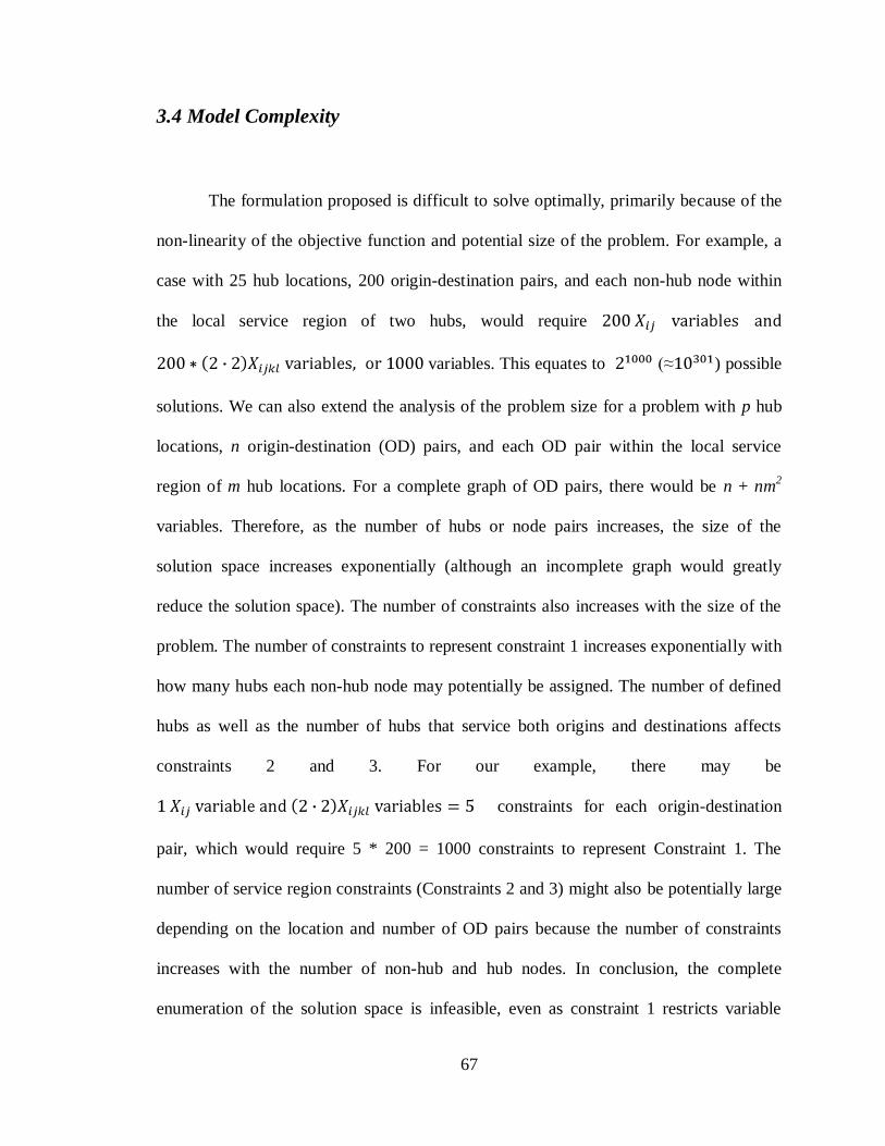
67
3.4 Model Complexity
The formulation proposed is difficult to solve optimally, primarily because of the
non-linearity of the objective function and potential size of the problem. For example, a
case with 25 hub locations, 200 origin-destination pairs, and each non-hub node within
the local service region of two hubs, would require
variables. This equates to (≈ ) possible
solutions. We can also extend the analysis of the problem size for a problem with p hub
locations, n origin-destination (OD) pairs, and each OD pair within the local service
region of m hub locations. For a complete graph of OD pairs, there would be n + nm2
variables. Therefore, as the number of hubs or node pairs increases, the size of the
solution space increases exponentially (although an incomplete graph would greatly
reduce the solution space). The number of constraints also increases with the size of the
problem. The number of constraints to represent constraint 1 increases exponentially with
how many hubs each non-hub node may potentially be assigned. The number of defined
hubs as well as the number of hubs that service both origins and destinations affects
constraints 2 and 3. For our example, there may be
constraints for each origin-destination
pair, which would require 5 * 200 = 1000 constraints to represent Constraint 1. The
number of service region constraints (Constraints 2 and 3) might also be potentially large
depending on the location and number of OD pairs because the number of constraints
increases with the number of non-hub and hub nodes. In conclusion, the complete
enumeration of the solution space is infeasible, even as constraint 1 restricts variable

68
assignment (if Xij is 1, then its counterpart, Xijkl, must equal 0 for any combination of hub
nodes k and l).
If the objective function were linear with respect to its variables and cost
components, the problem would be much easier to solve. However, Maximum (max) and
Ceiling ( ) operators provide for a non-linear objective function and solution space.
This behavior should not be overlooked. It is known that as the number of variables
increases, the number of local optima also increases. In addition, the relative size of each
flow path with respect to the vehicle capacity affects the consolidated truckload cost, and
the amount of nodes that act as both origin and destination affect the local transportation
cost components. The integration of these factors all affect the value of the objective
function.
A solution procedure that would efficiently solve such a non-linear Integer
Program is not well-documented. For example, exchange and improvement heuristics
were applied to the Quadratic Assignment problems of early p-hub network models.
Therefore, it may require a specialized heuristic or enumeration-based solution procedure
such as branch-and-bound or linear relaxation. For instance, using a possible relaxation of
the non-linear operators as fathoming criteria may provide good bounds. For instance, a
relaxation of the ceiling operator would provide non-integer number of truckloads
required. This method may be useful in cases where smaller vehicles can be utilized or
the frequency of consolidated truckload service can be easily adjusted in practice. A
relaxation of the maximum operator to over-count local transportation costs may be used
to give upper bounds. Other heuristic methods to solve the problem may include
assigning flow to consolidation hubs according to the ratio of its direct connection cost

69
and its total size. The structure and convexity of the problem should be studied in greater
detail to generate ideas of how to find good or optimal solutions.
Because the problem is difficult to solve directly as it is a binary integer program
with non-linear behavior, a different approach to solving the problem has been
developed, which focuses on hub to hub arc selection, hub to hub service level, and node
assignment decisions. A feasibility check, sub-problem optimization model, and
specialized solution methodology will attempt to take particular advantage of the problem
structure. By considering this problem structure, it is possible to reach theoretically
optimal solutions to the original problem, namely determining all cost-effective locations
to implement less-than-truckload consolidation.
3.5 Specialized Solution Methodology
Due to complexity concerns of the original model, a specialized methodology is
proposed to determine the optimal set of consolidation scenarios within a shipment
network and the optimal origin and destination node allocation policy for each scenario.
Once optimal solutions are found for each scenario, they will be integrated into a global
solution.
The procedure starts with a feasibility check that will significantly reduce the
solution space with regards to feasible hub-to-hub arcs and potential hub locations. The
method compares the total cost for direct connection service against the cost for
consolidated truckload service. If the total cost of direct connection for all flow paths
within the two hubs' service regions is less than the cost of one full truckload on that

70
path, there is no need for consolidation service between the two hubs. That is not to say
that either hub cannot be a future hub location, but the hub-to-hub arc will not be a
component of the optimal network.
The second stage of the procedure is an optimization routine that will determine
the optimal consolidated truckload service level between each hub to hub arc as well as
the node assignment policy for each origin and destination node within the service
regions of the hubs. Because we determined the set of hub to hub arcs that are not
feasible only when disregarding local cost, this routine will now consider all cost
components including local cost such that we might eliminate more hub to hub arcs or be
able to justify economical consolidation.
The last stage of the solution procedure compares each optimal solution of the
two-hub scenarios and determines the global optimal hub network by resolving any
duplicate origin and destination node-to-hub assignments that were included within our
local solutions. For relatively large-scale, yet sparse networks consisting of highly
dispersed origins and destinations and varying levels of shipment volumes, the proposed
methodology will be a very useful tool to pinpoint the specific lanes that will result in
significant and sustainable cost savings.
To begin the solution procedure, the set H(k) is defined as the set of all nodes
located within the boundary of the local service region of the potential hub location k,
according to the maximum-allowable service radius defined in the original problem. The
solution procedure that will solve the hub-and-spoke network problem includes the
following Stages:

71
Stage 1: Feasibility Check of Hub Arcs
Stage 2: Solve Sub-model for Remaining Hub Arcs
Stage 3: Resolve Conflicts of Duplicate Assignments
Stage 4: Integrate Local Solutions and Discount Duplicate Local Costs
Stage 1 of the solution procedure should be executed for all unidirectional 2-hub
pairs of the original problem. For example, if there are n potential hubs, then there are
n(n-1) different pairs that should be considered. After completing the feasibility check,
the optimization model should be solved for all remaining scenarios. Stage 3 is used to
resolve assignment conflicts when origins or destinations are part of multiple sub-
solutions. Stage 4 seeks to integrate the sub-solutions into a global solution and end by
identifying any duplicate local costs within the global solution.
3.5.1 Stage One: The Feasibility Check
Stage 1 of procedure consists of the feasibility testing for all two-hub pairs and their
respective hub arcs within the entire set of potential hub location. The purpose of this
procedure is to aid in determining the set of feasible locations for consolidation for
networks with sparse shipment locations of varying shipment quantity. If many areas of
high shipment volume exist, there will naturally be many such feasible consolidation
areas. However, for sparse networks, the procedure will eliminate many lanes, which
decreases the amount of effort needed to identify potentially beneficial opportunities. For
each set of hub nodes k and l, if , then there should be no

72
consolidated truckload service from hub k to hub l. This inequality compares the cost of
one consolidated truckload between two hubs with the total direct connection cost
between those hubs’ service regions.
Regardless of any local pickup cost or cost of multiple trips, if the total cost of
direct connection is less than even one truckload, we know there is no possibility for
consolidation to be advantageous at any truckload service level. This inequality will
always filter out infeasible solutions to the hub arc selection problem because the local
pickup or delivery cost will always be positive (regardless of local cost shared between
more than one flow path), and the frequency of consolidated truckload service might in
fact be greater than one trip per planning period (because of vehicle weight/volume
capacity constraints).
This feasibility check will determine which hubs and hub-to-hub arcs should still
be in consideration within an optimal network design. It is also important to note that a
specific hub can also be excluded from the potential optimal hub set if such a hub fails
for all of its own two-hub feasibility checks.
3.5.2 Stage Two: Solve Sub-Model for Remaining Two-Hub Scenarios
During Stage 2, a new mathematical model is formulated to determine which remaining
two-hub scenarios result in positive cost savings. The new formulation uses previously
defined flow paths (i, j) and node-to-node distances, as well as network cost parameters.
However, new variable Yi is a binary variable that equals 1 if i H(k) utilizes
consolidated truckload service and 0 otherwise. Zj is a new binary variable that equals 1

73
if j H(l) utilizes consolidated truckload service and 0 otherwise. Xijkl is defined as a
binary variable that equals 1 if the flow path (i,j) uses consolidated truckload service
through hubs k and l. Finally, n is defined as the service level variable which represents
the number of truckloads employed between the two hubs. The formulation is as follows:
Maximize
Subject to:
Although we consider the same cost components, the revised model differs from
the original model in many regards. First, the two objective cost components include the
direct connection cost for a given set of flow paths that utilize the given two-hub pair, the
consolidated truckload cost (dependent upon the variable service frequency and fixed
truckload cost parameter) and local pickup and delivery cost. We also notice that in this
formulation the local cost does not contain a maximum operator. When considering only
two hubs within the scenario, any origin or destination node can only be assigned to its
respective hub exactly one time, which leaves no opportunity for counting local cost
more than once.
The first constraint ensures that if a node pair does not use the hub nodes k and l,
then the nodes i and j do not use the truckload arc connecting the two hubs. The second

74
constraint requires that the total flow between all the origin nodes and destination nodes
within the two service regions of the hubs must be less than the available capacity of the
truckloads, given as the number of truckloads multiplied by each truck’s individual
capacity, w. Therefore, when a given number of truckloads limit the total flow available
for consolidation, the optimal decision will include which origins and destinations should
be included in truckload service.
If the optimal objective function value is positive, the cost of direct connection for
the set of origins and destination nodes within the local service region outweighs the cost
of local pickup and delivery and full truckload costs for a given number of truckloads
over the planning period. Therefore, it would be beneficial to use a consolidated full
truckload as opposed to direct connection.
Although the sub-model formulation remains an integer program, solving this
model is much easier than solving the original model. Because we originally assumed
that each set of hub-to-hub routes that share local service need to account for local cost
due to coordination and scheduling concerns, we do not need to worry about duplicate
local service costs. In addition, the integrality operator (ceiling) can be lifted by an
integer variable to determine the service level between each hub for consolidated service.
As each sub-problem only considers a unidirectional path between two hubs and
the feasible set of hub arcs will be considerably less than the original set of all hub arcs,
the solution space for the global solution of integrating each sub-problem is considerably
smaller than the original formulation. For example, a sub-problem with n origin nodes, n
destination nodes, m OD pairs, we would have only n Yi variables, n Zj variables, and m
Xijkl variables, which equals a total of (n+n+m) variables. If our original problem has

75
been reduced during the feasibility check to a set of q hub-to-hub arc routes, the number
of solutions for the global problem is q2(2n+m)
. With both linear objective functions and
constraints, the sub-model formulation is relatively easy to solve optimally.
Although the number of two-hub scenarios increases exponentially with the
number of potential hub locations, the feasibility check for each scenario can be run in
constant time. Therefore, it can be concluded that enumeration or heuristics are not
necessary to solve the original consolidation network design model due to a very
tractable sub-model formulation. In addition to finding optimal solutions, the specialized
methodology may have an added benefit of a much faster running time to solve the global
problem, given an automated version of the process.
The mathematical model proposed in Stage 2 can be solved by commercial
software packages such as LINGO that utilize a branch-and-bound procedure. If
necessary, the integer program may be changes to a binary integer program by converting
the integer variable n to its binary representation. This does not add a significant number
of variables because there is only one such n variable for each sub-problem.
Alternate Iterative Solution Method for Sub-Model
If preferred, the sub-model for each two-hub scenario may also be solved
iteratively, increasing the n variable by 1 for each iteration. In doing so, n will become a
defined model parameter. Sub-problems would begin by setting the n parameter to 0.
Depending on the relative size of shipment flow paths, if a point is reached when the
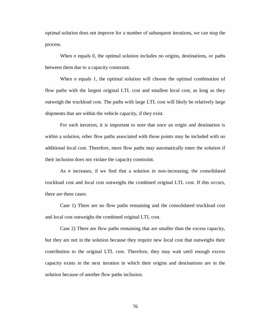
76
optimal solution does not improve for a number of subsequent iterations, we can stop the
process.
When n equals 0, the optimal solution includes no origins, destinations, or paths
between them due to a capacity constraint.
When n equals 1, the optimal solution will choose the optimal combination of
flow paths with the largest original LTL cost and smallest local cost, as long as they
outweigh the truckload cost. The paths with large LTL cost will likely be relatively large
shipments that are within the vehicle capacity, if they exist.
For each iteration, it is important to note that once an origin and destination is
within a solution, other flow paths associated with those points may be included with no
additional local cost. Therefore, more flow paths may automatically enter the solution if
their inclusion does not violate the capacity constraint.
As n increases, if we find that a solution in non-increasing, the consolidated
truckload cost and local cost outweighs the combined original LTL cost. If this occurs,
there are three cases:
Case 1) There are no flow paths remaining and the consolidated truckload cost
and local cost outweighs the combined original LTL cost.
Case 2) There are flow paths remaining that are smaller than the excess capacity,
but they are not in the solution because they require new local cost that outweighs their
contribution to the original LTL cost. Therefore, they may wait until enough excess
capacity exists in the next iteration in which their origins and destinations are in the
solution because of another flow paths inclusion.

77
Case 3) There are flow paths remaining that are more than the excess capacity,
but they are not in the solution because they violate the capacity constraint.
A good rule-of-thumb to find a good solution of this problem is created based on
the aforementioned problem behavior:
Rule. If a current solution is non-improving, we will increase n by one at most
times, where is the largest flow path remaining and w is the vehicle
capacity. If there are other flow paths remaining, then waiting for the largest flow path
will give all other flow the opportunity to enter an improving solution. Waiting the
additional iterations will allow the largest flow path the opportunity to create an
improving solution. The allowance for additional iterations will also give flow paths from
Case 2 the opportunity to find their respective origins and destinations within a solution.
If after the additional iterations, not one improving solution is found, the procedure is
ended and the best solution to date is used.
3.5.3 Stage Three: Resolve Duplicate Assignments
After all sub-problems from the set of potential hub-to-hub arc routes have been
optimized with respect to cost savings opportunity, the results must be further analyzed.
Depending on the problem data set, each origin or destination point may be within the
maximum allowable distance of more than one hub, for instance, when two potential
hubs have overlapping service regions that share certain origins or destinations.
Therefore, in our solutions, the same origin-to-destination path may be routed through
different hub sets. After solving each sub-problem, each scenario contained positive cost

78
savings; however, they shared one or more flow paths that contributed to the success of
each sub-problem. This is not in accord with the original model and should be resolved in
order to find feasible solutions to the optimal network design. Figure 3.1 shows this
scenario. Otherwise, if all flow paths are only components of one sub-solution, the
addition of all two-hub sub-solutions forms a globally-optimal solution.
Figure 3.3 Conflicting Sub-solutions
Depending upon the specific example case and original network configuration,
conflicts can occur in several situations when integrating the various two-hub solutions.
Conflicts occur when one or more origin-to-destination flow path is included within the
optimal solution for two or more unique sub-problems, with the possibility that one hub
is a component of all sub-problems.
When a unique flow path is shared by two optimal sub-solutions, the global
solution is impacted by the interactions of each sub-solution. The decision becomes what
is the optimal arrangement for the different origin and destination nodes and their
associated, directed flow paths. In this case, the path allocation problem becomes a
H2
D2
D1
O1
O2
H *
H

79
combinatorial problem itself. Figure 3.5 shows the flow paths shared for a conflict
instance.
Figure 3.4 Origin-to-destination Flow Paths within a Potential Conflicting Scenario
In most cases, the number of conflicting flow paths is small enough that it is
possible to enumerate each different solution with and without each specified flow path.
Scoring the objective function of each existing sub-problem solution simultaneously for
complementary assignments of the shared flow paths will determine which solution is
better. If the scenarios cannot share the shipments in a way that adding solutions would
exceed the best of the individual scenario solutions, the best existing scenario is chosen
and the other scenario will not consolidate and continue to employ less-than-truckload
transportation.
O2
O1
D1
D2
s11 s21
s12
s22

80
Figure 3.5 Conflict Resolution Chart for Four Shared Flow Paths
The enumeration process involves changing the value of the Xij variable
corresponding to each flow path sij within each existing scenario solution. If the absence
of the variable removes the origin or destination from the solution as well, then the
corresponding Y or Z variable should also be adjusted. Finally, the solutions are scored
with the existing objective function. The objective function values for each scenario with
complementary variable assignments are combined. Then, the best solution among the
maximum global solution and the maximum original sub-solution is chosen. Figure 3.5
gives an example of a conflict resolution procedure chart using the case described in
Figures 3.3 and 3.4.
For cases with several conflicting scenarios (more than two), it may suffice to
simply pick the scenario with the best solution and dismiss the others when there are
several shared flow paths. Other more complicated conflicts may require a small-scale
SCENARIO 1 SCENARIO 2 GLOBAL
S11 S12 S21 S22 OF 1 S11 S12 S21 S22 OF 2 OF1 + OF2
1 1 1 1 0 0 0 0
0 1 1 1 1 0 0 0
1 0 1 1 0 1 0 0
0 0 1 1 1 1 0 0
1 1 0 1 0 0 1 0
0 1 0 1 1 0 1 0
1 0 0 1 0 1 1 0
0 0 0 1 1 1 1 0
1 1 1 0 0 0 0 1
0 1 1 0 1 0 0 1
1 0 1 0 0 1 0 1
0 0 1 0 1 1 0 1
1 1 0 0 0 0 1 1
0 1 0 0 1 0 1 1
1 0 0 0 0 1 1 1
0 0 0 0 1 1 1 1

81
implementation of the global model in Section 3.3 and solved using non-linear techniques
or rounded solutions of its linear relaxation.
3.5.4 Stage Four: Integrate Local Solutions
At this point, it is important to recall that local costs for different two-hub scenarios do
not have to be discounted for duplicate local transportation because of coordination issues
between different consolidation scenarios. If desired, local costs may be discounted for
origin or destination nodes that are components of more than one sub-solution if the
scenarios have the same optimal service frequency, n. Resultantly, the individual
solutions for each two-hub pair and their corresponding hub arcs are mapped to the entire
network, complete with each non-hub node's assignment policy to its hub. A
consolidation network has now been created.

82
CHAPTER 4
CASE STUDY
Through detailed exploration of current literature and research, and the case of a
real less-than-truckload network of a U.S. manufacturer, it was determined that the case
fits the hub-and-spoke model very well. Therefore, the proposed model could be applied
to this particular situation in attempts to realize significant logistics cost savings. To
realize these savings, efforts can be concentrated on the large numbers of small, unique
LTL shipments for which the many example company branches are responsible every
day.
4.1 Company Background3
The example company was founded and became incorporated around the turn of
the 20th century. Now, this company is a diversified manufacturer that researches,
designs, and produces products for the home, office, and automobile industry.
The business is divided into many business units among several business groups
that comprise four unique segments. The company currently owns approximately 200
branch operations that represent manufacturing, warehousing, corporate, and
administrative operation. The first, and largest, segment consists of business units
producing bedding and furniture components, as well as fabric and foam products. The
3 Information current as of January 2008.

83
next segment includes groups that produce retail displays, storage products, and office
furniture components. Yet another segment consists of two groups that produce steel
wiring and tubing as well as other wire products for use throughout a variety of the
company's business segments. Finally, the last segment includes business groups that
produce automobile interiors and bodies as well as industrial machinery for the textile
industry, printing, and factory automation.
This company has also expanded its operations in North America to include
Mexico and Canada, and overseas to include Europe and Asia. Other facilities are located
in South America and South Africa.
The company currently employs approximately 33,000 employees, with the
majority working in production. Roughly one-third of employees are located
internationally and approximately fifteen percent of employees are represented by labor
unions.
4.2 Operations and Policy
With operations and markets in nearly all 48 contiguous states, the company
operates a very large scale domestic distribution network. This network is in charge of
delivering subassemblies, component goods, and finished goods to retailers and other
production facilities all throughout the country in a timely manner. To accomplish this
feat, both rail and road-based transportation is employed. Full-truckload (FTL or TL) and
rail transportation is primarily used for long-haul transportation and distribution of full
containers of goods produced in both its overseas and domestic production plants. Less-

84
than-truckload (LTL) is used to distribute smaller, specialized shipments between its
branch operations and suppliers, vendors, and other customers. Shipment destinations
may also include company branches and other private organizations with production
facilities of their own.
Truckload transportation accounts for approximately one-half of the total
shipments that the company is responsible for, which amounts to over 3000 per week.
Corporate management obtains visibility of these shipments due to the implementation of
a centralized transportation planning software, TMS (Transportation Management
System) to record, plan, and dispatch Full Truckload transportation. In total, there are
estimated over 600 TL carriers utilized throughout the U.S. to serve company truckload
transportation needs.
Less-than-truckload accounts for the other approximate half of road transportation
with an estimated 3000 to 4000 shipments per week. Corporate headquarters currently
has nearly complete visibility of branch LTL shipments due in part to a recent centralized
initiative to decrease the number of less-than-truckload carriers for domestic branches to
just a small number of core carriers, which requires high branch compliance. The
impressive corporate visibility results from information sharing and data collection of
LTL shipment history into a centralized database. Through this process, corporate
management also records the many different properties of LTL shipments.
The company currently uses the industry-standard Czar freight rating software
for less-than-truckload transportation pricing. The shipper uses the Czar program to find
the rate of an LTL shipment by inputting zip codes of origin and destination as well as
weight (in pounds) and the class of the shipment. There are also opportunities to input the

85
agreed carrier discount, minimum charges, accessorial charges, etcetera, per the FAK.
The FAK (Freight of All Kind) contains important details about the agreements the
company has with the core LTL carriers. This information includes LTL rate discounts
for each carrier as well as the policy on accessorial charges for specialized services and
exceptions to the base rate.
Outside of utilizing public, commercial TL and LTL carriers, the company owns
and leases a significant amount of freight vehicles and trailers to partially satisfy other
transportation needs. Each company branch is given a certain amount of trucks and
trailers for private use. Apart from branch transportation resources, the company also
owns and operates its own transportation company, an operation that operates like other
commercial TL carriers, with service many company branches. This transportation
company owns a relatively smaller fleet with the majority of resources based in the
Southern and Midwestern United States.
4.3 Data provided
A large amount of data and information describing the many facets of regulation,
corporate policy, and operations was provided by the company.
The most important source of data was the LTL History Database, a Microsoft
Access database file of all the Less-than-truckload shipments of which corporate had
visibility beginning March, 2006 and ending June, 2007. The database includes all North
American shipments for all branches. The shipment history database includes information
on shipment date, carrier used, processing date, branches involved, origin City, State, and
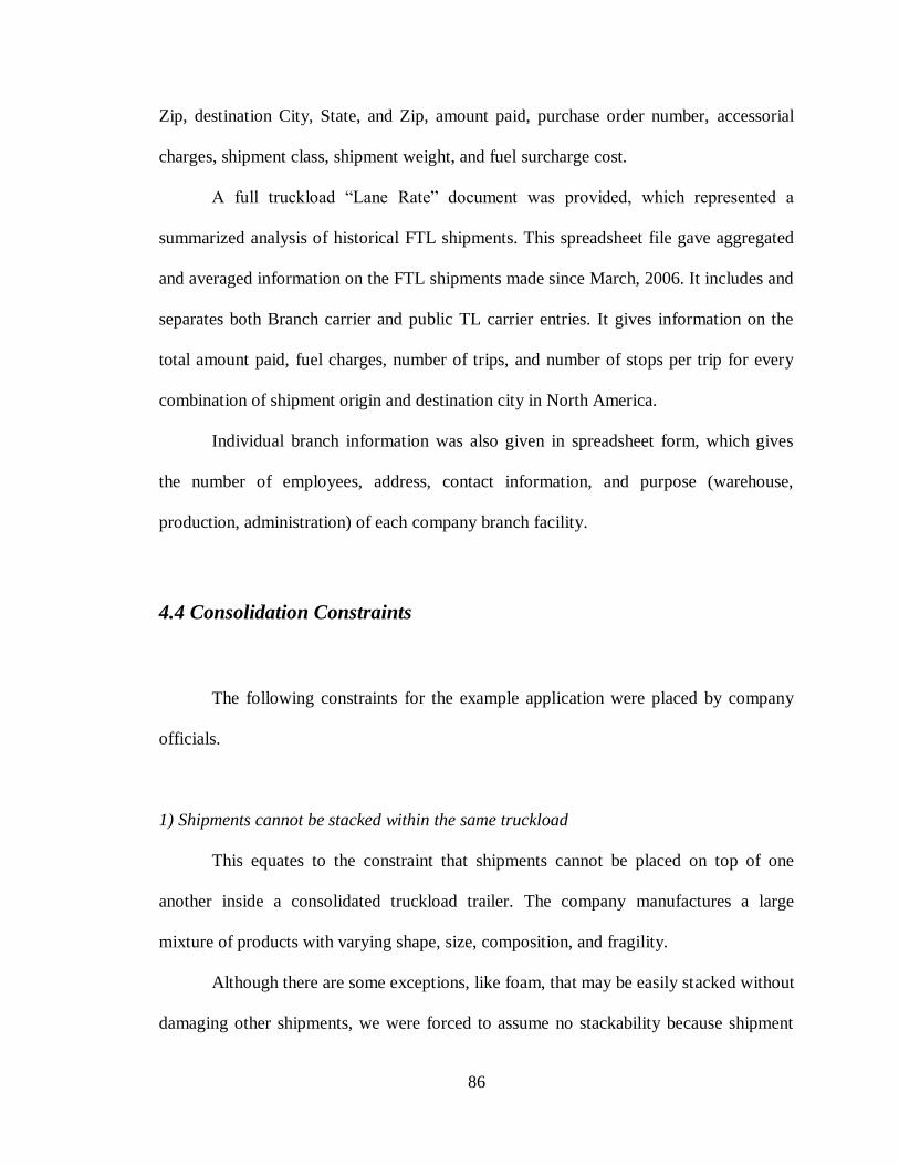
86
Zip, destination City, State, and Zip, amount paid, purchase order number, accessorial
charges, shipment class, shipment weight, and fuel surcharge cost.
A full truckload “Lane Rate” document was provided, which represented a
summarized analysis of historical FTL shipments. This spreadsheet file gave aggregated
and averaged information on the FTL shipments made since March, 2006. It includes and
separates both Branch carrier and public TL carrier entries. It gives information on the
total amount paid, fuel charges, number of trips, and number of stops per trip for every
combination of shipment origin and destination city in North America.
Individual branch information was also given in spreadsheet form, which gives
the number of employees, address, contact information, and purpose (warehouse,
production, administration) of each company branch facility.
4.4 Consolidation Constraints
The following constraints for the example application were placed by company
officials.
1) Shipments cannot be stacked within the same truckload
This equates to the constraint that shipments cannot be placed on top of one
another inside a consolidated truckload trailer. The company manufactures a large
mixture of products with varying shape, size, composition, and fragility.
Although there are some exceptions, like foam, that may be easily stacked without
damaging other shipments, we were forced to assume no stackability because shipment

87
information about product or material was not given within the provided data. Therefore,
there would be no way for us to prohibit, for example, a glass fixture or automotive
component being stacked on top of anything else. There may be the opportunity including
stackability issues in extended models.
2) Individual pieces are to be combined as one shipment, with the measure (weight,
volume, etc.) of the combined shipment as the sum of the individual orders.
This assumption was important to make for cases when shipments originating
from the same location, processed on the same date, and travelling to the same
destination contains multiple pieces that vary in class, weight, or other properties.
3.) No capital cost can be incurred for hub construction, retro-fitting, storage space, and
material handling.
The company cannot build new facilities for warehousing or consolidation.
However, existing warehouses, distribution centers, or manufacturing facilities are
capable housing consolidation operations, with preference given to utilizing existing
warehouses or distribution centers rather than production facilities. Therefore, the
example application case will place hubs in existing facility locations.
4.5 Data Preprocessing
Before we were able to analyze the data, we filtered to include only the most
relevant data. This equated to removing shipments within the LTL shipment history that

88
indicated for what the company was not responsible for paying, all shipments that
included either origins or destinations outside of the United States, as well as expedited
shipments, because those are not capable of being held extended periods of time for
consolidation. Other measures were taken to format the given data in a way that would
permit its use within the proposed mathematical model.
4.5.1 Defining the Unit for Shipment Flow
When consolidating unique shipments with varying dimensions of weight and volume,
full truckloads are frequently filled to capacity with respect to one such measure before
another. Assuming no stackability, the two units that determine the number of vehicles
necessary to provide truckload service are weight and the floor-space of the vehicle
storage container. The question that has to be answered is which factor will limit the
utilization of a full truckload more. Characteristics of the individual shipments
determined that weight was not the most accurate unit to define the combined size of
consolidated shipments. Therefore, each shipment flow path was converted to an
estimated measure of volume and surface area.
To convert each shipment to volume and vehicle floor-space utilization, both the
class and weight given within the LTL history database were converted using a density
factor specific to each class. The density factors were ascertained from the National
Motor Freight Classification (NMFC) Committee Density Guidelines described the
relationship between freight class and shipment density. The estimation for vehicle floor-
space utilization is as follows:

89
Truck Space Utilization (%) = (Shipment weight/ Shipment density) 2/3
/ 424
Dividing the shipment weight by the shipment density will give an estimation of
the shipment volume, which assumes a strictly cubic shape with equal dimensions.
Calculating the cubic root of this value will result in the length of each dimension.
Squaring this result will then determine the approximate surface area of a shipment.
Finally, dividing the surface area by the surface area of a standard trailer of 53 foot length
and 8 foot width will determine the percentage of truck space that each shipment will
consume.
Class Density
(lbs/ft3) Conversion Factor
Class Density (lbs/ft3)
Conversion Factor
50 55 .018 110 8.5 .118
55 42.5 .024 125 7.5 .133
60 32.5 .031 150 6.5 .154
65 25 .040 175 5.5 .182
70 20 .050 200 4.5 .222
77.5 15 .067 250 3.5 .286
85 13 .077 300 2.5 .400
92.5 11.5 .087 400 1.5 .666
100 10 .100 500 1 1
Figure 4.1 Density Conversion Factors for Shipment Classes
It was determined that volume and vehicle floor-space would be used to describe
the size of shipments after analyzing the LTL shipment data. Because shipment weights
were provided, it was possible to compare the combined weight to the estimated vehicle
utilization for each shipment path between two zip codes. Out of 2,730 records of
90
shipments, approximately 84 percent filled truckload floor-space capacity before weight
capacity was filled. When analyzing the top 450 shipment "lanes" estimated larger than 1
truckload, truckloads were filled quicker using floor-space utilization by an average of .8
truckloads. This analysis reveals that shipments are generally lower density items.
Therefore, using vehicle floor-space utilization is a more fitting unit of measure for less-
than-truckload shipments.
4.6 Less-than-truckload Network
As described in the previous sections, the LTL shipment data provided was
converted from class and weight to the proportion of a common freight trailer. With all
shipments converted, we examined the current LTL transportation network at a high level
to check for any clear opportunities for LTL consolidation. Aggregating the data on the
state, city, and zip code levels and mapping the data were all great tools for representing
the shipment data and identifying areas with high potential for transportation cost savings
through consolidation.
When trying to determine where to consolidate LTL shipments using the hub and
spoke model, the very large lanes typically present themselves clearly simply through
numbers. For areas with very large shipment volumes relative to vehicle capacity and
very high costs of shipping relative to consolidated, truckload shipping are clear areas to
consolidate with high potential for cost savings. These areas can be determined from
simply aggregating the shipment date at the city level and comparing LTL shipment
volume and cost figures against the corresponding consolidated truckload estimates.

91
However, for well-distributed shipment origins and destinations of relatively smaller-
volume shipping lanes, it is harder to "eye-ball" the situation.
The analysis began by examining the existing transportation network and flow of
goods, and several things stood out. First, it was apparent that the network was indeed
very well distributed but also sparse in terms of significant lanes of LTL shipments.
Varying levels of shipments originate from places all around the United States, but larger
single shipment "lanes" are only originating in select locations. Considering that the data
included all shipments within a 65 week period and no one city-level shipping lane
included more than 18 estimated truckloads, there were no clear opportunities for weekly
consolidating policy by simply looking at the numbers. Assuming a truckload was
dispatched once per week, this lane would utilize approximately 28% of each truckload.
By analyzing the numbers and viewing a map of the shipping lanes, it was
apparent that many areas appeared to be good candidates for consolidation. Places that
contained a large amount of originating shipments included the Los Angeles area, the
Dallas/Ft. Worth area, Denver, several cities within North Carolina, Atlanta, Chicago,
Carthage, Tupelo, among others. These origins generally align with the location of
company production facilities and/or warehouse facilities. Destinations are much more
distributed throughout the United States. However, Florida did stand out as a state that
had no significant production but very highly distributed consumption. This may imply
that the state is a bad candidate for consolidation efforts, due to a high cost of local
pickup and delivery cost for any hub and hub service region and increased truckload rate
to make up for relatively empty back-haul.

92
Other noticeable behavior of the company's LTL network was the abundance of
one-way transportation lanes and noticeable lack of areas that contained large amounts of
both origins and destination. Typically, bi-directional routes are preferable over uni-
directional routes due to the potential for fully utilized back-haul trailers, which
encourage lower rates, and dedicated trucking service, which improve driver satisfaction
and route management.
Figure 4.2 shows a pictorial representation of the major origin and destination
points within the example company's less-than-truckload network.
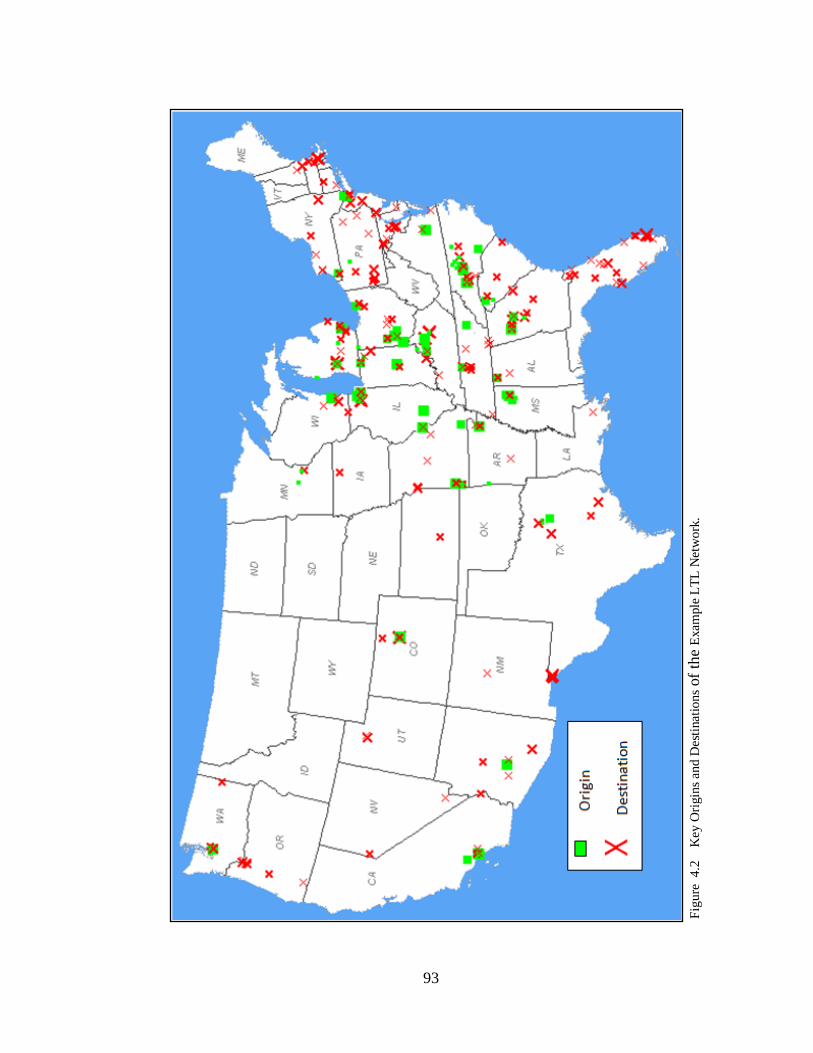
93
Fig
ure
4.2
K
ey O
rigin
s an
d D
esti
nat
ion
s of
the
Exam
ple
LT
L N
etw
ork
.

94
CHAPTER 5
EXAMPLE CASE AND RESULTS
To illustrate the mathematical modeling and solution approach proposed in this
research, an example case will be solved with data provided by the example company.
With thousands of shipments being transported every year between many unique origins
and destinations and little branch coordination, the company is a good candidate for a
shipment consolidation policy.
5.1 Model Parameters
5.1.1 Set of Origin and Destination Nodes and Flow Paths
Origin-to-destination flow paths were defined using the converted shipment quantities
from the provided less-than-truckload shipment data. Flow values and original LTL costs
were aggregated at the 5-digit zip code level. Therefore, these zip codes also defined the
individual origin and destination nodes.

95
Figure 5.1 Origin and Destination Flow Paths with Aggregated Flow
5.1.2 Potential Hub Locations
For the general case, the company employing the proposed model is capable of defining
the set of potential hub locations in whatever way it sees fit. In fact, the model is capable
of adding a cost component to account for hub opening, construction, or operating costs.
However, per consolidation constraints, potential hub locations in this case will be
existing company facilities, whether production or distribution centers, that are located
nearly relatively clustered areas of origin or destination points. These areas were chosen
by studying Figure 4.2 and reviewing other company data. Therefore, potential hub
locations were chosen from existing facilities with no hub costs. To illustrate the model's
effectiveness to a general scenario, the set of potential hubs was also chosen semi-
arbitrarily from the entire set of origin and destination nodes.

96
Figure 5.2 Locations of Potential Hub Facilities
Figure 5.3 List of Hub and Non-hub Nodes within each Local Service Region.

97
Once hubs were chosen, the set of origin and destination nodes were filtered
based upon the distance from nearby hub locations. In accord with the model definitions
and constraints, only nodes within the local service region of a hub are considered. In this
case, the local service region was set to 50 miles. Figure 5.3 shows the set of nodes
within each hub's service region.
5.1.3 Hub-to-Node and Hub-Hub Distances
All distances between both hub and non-hub nodes were found using the on-line mapping
site MapQuest, a web query, and VBA macro within Microsoft Excel. In doing this,
distances were estimated along common interstate highway and local routes. The
following figure shows the web query code used with Excel.
Figure 5.4 Web Query to Calculate Distance between Nodes

98
5.1.4 Redefining Original LTL Costs
As previously defined in the mathematical models, sij and cij represent the flow measure
and cost per unit flow for LTL shipments, respectively. However, we know the rates of
LTL shipments to be dependent on multiple factors such as weight and class values.
While it may be possible to loosely approximate a cost per pound or cost per shipment
based on class, it would be much more difficult to approximate and evaluate a cost
function based on multiple factors.
By using historical data, there is no need to define the cost function at all.
Specifically, the aggregated amount paid by a company along a given flow path should
encompass all information about the relationship between cost, weight, class, and any
other factors. Therefore, we can ignore the cost function altogether, given that the
underlying dependencies between cost and factors like weight or class will not change
during the future. We can then redefine direct connection costs as the historical aggregate
value and use this value as the basis of comparison against a consolidation policy. Using
historical data will be better than any approximation because it contains the true behavior,
so long as the time period for aggregating historical data is the same for the planning
period for full truckload service.
After redefining the costs for direct connection, a new aggregate LTL cost is
defined as ij, which will replace the product of the cost parameter, cij, and the flow
value, sij, for each flow path (i,j). Even after removing the need for sij within the direct
connection term of the objective function, sij is still used to calculate the cost of

99
consolidation because the total flow and truck capacity will determine how many full
truckloads are needed between two hubs throughout the planning period.
5.1.5 Other Model Parameters
Because the provided cost and shipment quantity data was aggregated for a 65 week
period, the scalar amount (65) was used throughout the mathematical formulation to scale
relevant costs, such as the consolidated truckload cost and the local pickup and delivery
costs. These costs were defined as a fixed cost per occurrence. Due to the aggregated
period of 65 weeks, these costs needed to be adjusted to make a fair comparison with
historical values.
The local cost parameter included a 4 dollar per gallon fuel charge (in accordance
with national average fuel price) and a vehicle fuel economy of 7 miles per gallon.
Truckload cost was the grand historical average for all shipments made during the same
65 week period, estimated as a $1.50 per mile effective rate.
5.2 LINGO Model
The proposed mathematical model was coded to be solved by the LINGO
optimization software package. LINGO uses a branch-and-bound procedure to determine
the optimal variable decisions and calculates the optimal objective function, complete
with reduced costs for decision variables. The following figure shows the code used to
implement the proposed model.

100
Figure 5.5 LINGO Code
5.3 Case Results
Stage1 of the solution procedure (The Feasibility Check) was implemented in
Microsoft Excel by comparing the aggregated LTL shipment cost matrix with the
estimated consolidated truckload cost matrix at a service level of one truckload per week.
The feasibility check determined which hub to hub scenarios should be considered as
further potential consolidation scenarios. Sample results are shown in the following
figure.

101
Figure 5.6 Excel Feasibility Matrix
After completing the feasibility check, there were 27 candidate scenarios that
were solved using the optimization model. These scenarios can be seen in Figure 5.7. For
each of the 27 two-hub scenarios, the relevant mathematical model parameters were
defined.
Figure 5.7 Resulting Scenarios after Stage 1: Feasibility Check
Origin Hub
Destination Hub

102
Figure 5.8 Example Spreadsheet for sub-problem between Zip Codes 32837 and 30012
Microsoft Excel was used to input the appropriate data within LINGO
optimization Software. Figure 5.8 shows an example spreadsheet used within Stage 2 to
solve each sub-model. With the input data properly defined for each potentially-optimal
scenario, LINGO was used to determine if each sub-problem results in positive cost
savings in a consolidation network configuration.
LINGO was used to optimize all 27 consolidation scenarios. If the optimal
objective value was positive, the solution reflected a clear opportunity for cost savings
through consolidation. The following figure shows example results from one such sub-
problem. An objective function value greater than zero indicated that consolidation of the
specified non-hub locations results in a cost that is cheaper than using less-than-truckload
for each associated shipment. The optimal service level is also determined to be one
truckload per week. LINGO results also show the individual origin and destination node
assignment policy, represented by X, Y, and Z variables.

103
Figure 5.9 Example LINGO Results
Confidential

104
After solving each sub-problem during Stage 2, there were 9 scenarios that
resulted in positive costs savings. However, two such scenarios included four common
origin-to-destination shipment flows. While there were several other instances where
more than one service regions overlapped, none of these instances resulted in a conflict of
cost-saving solutions.
Resultantly, Stage 3 was employed to determine if there is an effective way that
both scenarios can share the shipment flow and remain cost-saving scenarios. Figure 5.9
shows the two scenarios and the overlapping service regions, which includes two nodes
that are components of two different solutions.
Figure 5.10 Conflicting Solutions

105
Stage 3 was then employed to determine the optimal policy for each of the two
previous solutions that wrongly include four common shipment flows. The objective then
was to determine if both solutions can withstand a distribution of the common shipment
flow and remain cost-saving scenarios. If the scenarios cannot share the shipments in a
way that integrating solutions would exceed either scenario, the scenario with larger cost
savings is chosen and the other scenario will continue to employ less-than-truckload
transportation.
The method used to solve this problem was enumeration of the possible ways to
distribute the common shipments. The enumeration was completed in Microsoft Excel by
changing the value of each Xij variable (and Y or Z variable, if necessary) within each
solution. The following figures show the results of the enumeration process.
Figure 5.11 Scenario 1 Variable Assignments and Objective Function Values

106
Figure 5.12 Scenario 2 Variable Assignments and Objective Function Values
After enumerating the various assignments, it was determined that the two
scenarios could not share the four shipment flows and both remain cost-saving scenarios.
Therefore, it was determined that Scenario 2 resulted in the largest cost savings and was
chosen as a component of the resulting global solution. Figure 5.12 shows the various
locations for hub locations within the global solution.
Figure 5.13 Hub Locations in the Global Solution
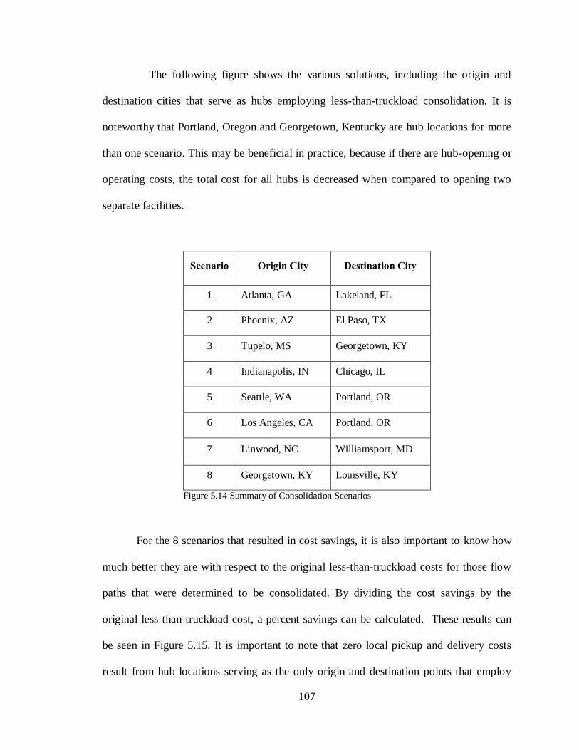
107
The following figure shows the various solutions, including the origin and
destination cities that serve as hubs employing less-than-truckload consolidation. It is
noteworthy that Portland, Oregon and Georgetown, Kentucky are hub locations for more
than one scenario. This may be beneficial in practice, because if there are hub-opening or
operating costs, the total cost for all hubs is decreased when compared to opening two
separate facilities.
Scenario Origin City Destination City
1 Atlanta, GA Lakeland, FL
2 Phoenix, AZ El Paso, TX
3 Tupelo, MS Georgetown, KY
4 Indianapolis, IN Chicago, IL
5 Seattle, WA Portland, OR
6 Los Angeles, CA Portland, OR
7 Linwood, NC Williamsport, MD
8 Georgetown, KY Louisville, KY
Figure 5.14 Summary of Consolidation Scenarios
For the 8 scenarios that resulted in cost savings, it is also important to know how
much better they are with respect to the original less-than-truckload costs for those flow
paths that were determined to be consolidated. By dividing the cost savings by the
original less-than-truckload cost, a percent savings can be calculated. These results can
be seen in Figure 5.15. It is important to note that zero local pickup and delivery costs
result from hub locations serving as the only origin and destination points that employ

108
shipment consolidation. The following costs and cost savings are normalized on a 100-
point scale to ensure privacy of information. It is also important to note that the amount
of original LTL cost varied for each scenario, which translates into different absolute
measures of cost savings for each scenario.
Scenario Original
LTL Cost
Truckload
Cost
Local
Cost
Cost Savings
1 100 61 21 19
2 100 80 0 20
3 100 69 14 17
4 100 87 0 13
5 100 81 9 10
6 100 88 10 2
7 100 79 18 3
8 100 92 0 8 Figure 5.15 Summary of Savings
109
CHAPTER 6
CONCLUSIONS
6.1 CONCLUSIONS
In our particular case, we must also be very aware of the limitations of this
application with respect to the nature of less-than-truckload shipping. The stochastic,
random, and intermittent nature of less-than-truckload shipments and demand
significantly affects the ability to consolidate enough shipments within a given time
frame without excessive waiting time. For example, some time periods will require more
vehicles than others due to demand spikes or seasonality. Likewise, less-than-truckload
shipment composition and properties also behave randomly, which affects the potential to
fully utilize consolidated truckloads. Sometimes, shipments will include higher
proportions of denser items that reach a truck’s weight capacity, while other times truck
volume limits may be met before the weight limit. In our particular case, we are also
using a simple, but rough approximation of shipment size from a conversion of class and
weight. It is important to note that the estimations were not compared to real products to
determine if they misrepresent actual shipment sizes.
Without directly addressing all of these important issues within the mathematical
model, we believe we can still develop a model and solution procedure that can be
implemented successful for many cases, including the case example. Although it is
certain that the optimal design of the propose hub network model will not always operate

110
optimally at all points throughout the life of the network and the optimal solution and
cost savings values will not be realized on a constant basis, the value of our specialized
formulation and solution methodology will be in determining the most beneficial set of
lanes and hubs can result in transportation cost savings through shipment consolidation.
In research and industry, it has been described that logistics decisions can most
often be classified according to the scope of the decision. The first type of decision is the
strategic decision, which typically involves a planning horizon measuring in years. Such
decisions include logistics network design and procurement of costly resources (facility
location, facility layout, fleet sizing). These decisions are often based on forecasts and
estimated data. The second type of decision is the tactical decision, with the planning
horizon shortened to a matter of months. These decisions typically include production
and distribution planning (order picking methods, material handling systems, certain
consolidation strategies). The last classification of logistics decisions is the operational
decision, measured on a daily basis or even in real time. These decisions include vehicle
dispatching or order picking, and typically require detailed input data [13].
The proposed models are intended to be considered by the company on a strategic
level. In particular, the model proposed is tailored to cases in which it is relatively
unknown whether the existing less-than-truckload network provides ample shipment
volumes to ensure regular and frequent consolidated truckload service. While many of
the previous hub network models are very good tools for consolidation network
decisions, they are more realistic in cases when shipment volumes will fully utilize
truckload capacity, which justifies the included discount factor.

111
The results of the example case exhibited the value of the proposed methods to
identify areas for logistics and transportation cost savings through less-than-truckload
consolidation. In total, eight consolidation scenarios were identified to save transportation
costs when compared to previous less-than-truckload transportation. The specialized
methods of solving each hub-to-hub route separately also provide the opportunity for
sensitivity analysis with respect to important regional less-than-truckload and truckload
cost parameters.
Reviewing the percent savings of each scenario reveals that the most significant
scenarios with respect to absolute savings also carry high percent savings, as large as 20
percent. From a practical perspective, these results are very reasonable and encouraging.
Although issues like seasonality, stochasticity, and the fixed and operating costs of
consolidation affect the true savings that would result from a shipment consolidation
policy, high percent savings support the conclusion that the model identifies significant
areas for cost savings through consolidation.
Other issues also affect the extent to which the solutions to these proposed models
will perform over time. As markets and demand change, the configuration of the
consolidation network should change as well. When using the underlying model,
assuming purely one-way, two-hub arcs for consolidation, the opportunity exists to add or
subtract specific consolidation scenarios from the existing network. Assuming drastic
changes to demand would not go unnoticed, the network can be altered or the model can
be reevaluated with updated data at any time.

112
6.2 Extensions
Many extensions to the models and methods presented in this work are possible,
with varying levels of complexity and practicality.
The first area for extension is the inclusion of a cost term for customer
dissatisfaction or inventory holding, which would penalize excess waiting time for
shipment consolidation. Although the proposed formulations do not include time-based
components, the service level n is a measure of how often consolidated truckloads service
each hub. Thus, this parameter implicitly describes the service level for consolidation
routes because as n increases, more frequent service is being performed, which would
decrease the waiting time of shipments, customer satisfaction level, and inventory
holding costs. However, the exact relation between the service level parameter and these
effects is not defined explicitly through any mathematical function. By defining a cost for
each flow path that is proportional to the value of n, such costs would add practicality to
the solutions found and potentially prove prior solutions to be infeasible. In this way, the
cost component for excess waiting time could also reflect inventory holding costs.
Another important area for model extension is the inclusion within both the base
model and the specialized solution methodology for multiple capacity constraints. Due to
government regulations and vehicle capabilities, the vehicles used in freight
transportation have weight restrictions as well as the physical space constraints of a
trailer. Therefore, the models proposed in this research should include mathematical
constraints on both volume and weight. While the example case supported the

113
assumption of just one volume-based constraint, a generalized model should include both
constraints to be considered complete.
In the majority of current literature, weight is assumed the most determining
factor in consolidating shipments into one truck. Less often volume is used. Because the
proper data was supplied, it is possible to use weight as the determining factor if we
assume that weight capacity is met before volume. However, we have also been supplied
class information for each shipment, which makes it possible to compute an
approximation of shipment volume as well.
The next area for extension is the use of stochastic functions to describe shipment
composition within each origin-to-destination flow path. In current research, including
the proposed models, shipment flow quantities are deterministic. In fact, the proposed
models used aggregated data over the course of more than one year. In doing this,
seasonality and the intermittent and stochastic nature of less-than-truckload demand was
ignored. With shipment sizes and arrivals represented probabilistically, the model could
better describe the process of consolidating multiple sources of shipments with varying
size and quantity. By identifying periods of time that do not sufficiently utilize vehicle
capacity (which less efficiently shares transportation cost), there is the ability to
determine which time periods will effectively use consolidate shipments and which time
periods should not employ these methods. Such stochastic models could be solved in
terms of minimizing total cost while also probabilistically satisfying a defined service
level.
The inclusion of other consolidation strategies with respect to underlying hub-
and-spoke design is another opportunity. The proposed model assumes a traditional hub-
114
and-spoke design with a defined local service region, which was set in the example case
to 50 miles. Other research has used both defined and unlimited hub service regions.
There are clear opportunities to employ both multiple-assignment policies (routing a flow
path from origin to destination through more than two hubs) and the expansion of hub
regions to include both local pickup and delivery and further LTL services. Although the
models propose (assuming a simple hub-and-spoke design) are adequate in identifying
clear opportunities for consolidation, extensions to the model may identify much less
obvious configurations that would allow for very high vehicle utilization, thus, sharing
the cost of transportation among larger quantities of shipments. This would potentially
greatly increase the level of cost savings achieved.
Unfortunately, a multiple hub assignment policy would require the elaboration of
the first model proposed in this research, which was very complex in its structure. The
use of model decomposition such as the specialized methodology proposed may be
infeasible as a tool because of the many interactions that various origin-destination flow
paths would likely have within an optimal configuration. For the addition of less-than-
truckload transportation service at each hub, considerably more node-to-node distances
and cost parameters would need to be defined. However, a specialized methodology
similar to the one proposed in this research could also solve such a problem.
Finally, the opportunity exists to apply vehicle routing algorithms or
approximations to local pickup and delivery functions within the solution methodology or
after local two-hub solutions have been integrated. It may also be beneficial to reward the
assignment of nodes to hubs according to how close they are to one another.

115
BIBLIOGRAPHY
1. Bookbinder, J., and J. Higginson (2002). Probabilistic modeling of freight
consolidation by private carriage. Transportation Research-Part E, 38, 305-318.
2. Brimberg, J. et al. (2001). Improvements and comparison of heuristics for solving
the uncapacitated multisource Weber problem. Operations Research, 48 (3). 444-
460.
3. Brown, G.G. and Ronen, D. (1997).Consolidation of customer orders into
truckloads at a large manufacturer. Journal of the Operational Research Society,
48. 779-785.
4. Campbell, J. (1996). Hub location and the p-hub median problem. Operations
Research, 44(6), 923-935.
5. Campbell, J. (2005). Hub Arc Location Problems: Part 1-Introduction and Results.
Management Science, 51 (10), 1540–1555.
6. Campbell, J. (2005). Hub Arc Location Problems: Part 2-Formulations and Optimal
Algorithms. Management Science, 51(10), 1556–1571.
7. Cetinkaya, S. and J. Bookbinder (2003). Stochastic models for the dispatch of
consolidated shipments. Transportation Research-Part B, 37. 747-768.
8. Cooper, M. (1984). Cost and Delivery Time Implications of Freight Consolidation
and Warehousing Strategies. International Journal of Physical Distribution and
Logistics Management, 14 (6), 47-67.
9. Crainic, T.G. (2000). Service network design in freight transportation. European
Journal of Operational Research, 122 (2), 272-288.
10. Cunha, C.B. and M.R. Silva (2007). A genetic algorithm for the problem of
configuring a hub-and-spoke network for a LTL trucking company in Brazil.
European Journal of Operational Research, 179. 747-758.
11. Fleischmann, B. et al. (1998). Advances in Distribution Logistics. Berlin: Springer.
12. Ghiani, G. et al., Eds. (2004). Introduction to Logistics Systems Planning and
Control. New York: Halsted Press (Wiley).
13. Higginson, J. (1995). Recurrent decision approached to shipment-release timing in
freight consolidation. International Journal of Physical Distribution and Logistics
Management, 25 (5), 3-23.

116
14. Higginson, J. and Bookbinder, J. (1994). Policy recommendations for a shipment-
consolidation program. Journal of Business Logistics, 15 (1), 87-112.
15. Jackson, G. (1981). Evaluating order consolidation strategies using simulation.
Journal of Business Logistics, 2 (2), 110-138.
16. Jackson, G. (1986). A survey of freight consolidation practices. Journal of Business
Logistics, 6 (1), 13-34.
17. Kara, B.Y. and B.C. Tansel (2003). The single-assignment hub covering problem:
Models and linearizations. Journal of the Operational Research Society, 54. 59-64.
18. Klincewicz, J.G. (1990). Solving a Freight Transport Problem using Facility
Location Techniques. Operations Research, 28 (1), 99-109.
19. Klincewicz, J.G. (1991). Heuristics for the p-hub location problem. European
Journal of Operational Research, 53. 25-37.
20. Koskosidis, Y.A. and W.B. Powell (1992). Clustering algorithms for consolidation
of customer orders into vehicle shipments. Transportation Research-Part B, 26 (5),
365-379.
21. Lapierre, S. et al. (2004). Designing Distribution Networks: formulations and
Solution Heuristic. Transportation Science, 38 (2), 174-187.
22. Lium, AG. et al. (2006). Stochastic service network design: the importance of
taking uncertainty into account. Advanced OR and AI Methods in Transportation,
758-763.
23. Min, H. (1996). Consolidation terminal location-allocation and consolidated routing
problems. Journal of Business Logistics, 17 (2), 235-254.
24. Masters, J. (1980). The effects of order consolidation on customer service. Journal
of Business Logistics, 2 (1), 55-74.
25. Mayer, G. and B. Wagner (2002). HubLocator: an exact solution method for the
multiple allocation hub location problem. Computers and Operations Research, 29.
715-739.
26. O'Kelly, M.E. (1986). The Location of Interacting Hub Facilities. Transportation
Science, 20(2), 92-105.
27. O'Kelly, M. E. (1987). A quadratic integer program for the location of interacting
hub facilities.” European Journal of Operational Research, 32, 393-404.

117
28. O'Kelly, M.E. and D.L. Bryan (1998). Hub location with flow economies of scale.
Transportation Research-Part B, 32 (8), 605-616.
29. Pirkul, H. and D.A. Schilling (1998). An Efficient Procedure for Designing Single
Allocation Hub and Spoke Systems. Management Science, 44 (12), S235-S242.
30. Pooley, J., and Stenger, A. (1992). Modeling and evaluating shipment consolidation
in a logistics system. Journal of Business Logistics, 13 (2), 153-174
31. Popken, D. (1994). An algorithm for the multi-attribute, multicommodity flow
problem with freight consolidation and inventory holding costs. Operations
Research, 42 (2), 274-286.
32. Skorin-Kapov, D. et al. (1995). Lower Bounds for the Hub Location Problem.
Management Science, 41 (4), 713-721.
33. Sung, C.S. and W. Yang (2006). An exact algorithm for a cross-docking supply
chain network design problem. Journal of the Operational Research Society, 1-18.
34. Sung, C.S. and H.W. Jin. (2001). Dual-based approach for a hub network design
problem under non-restrictive policy. European Journal of Operations Research,
132. 88-105.
35. Wagner, B. (2007). An exact solution procedure for a cluster hub location problem.
European Journal of Operational Research, 178. 391-401.
36. Wagner, B. (2007). Model formulations for hub covering problems. Journal of the
Operational Research Society, 1-7.
37. Yoon, M.G. and J. Current (2006). The hub location and network design problem
with fixed and variable arc costs: formulation and dual-based solution heuristic.
Journal of the Operational Research Society, 1-10.